INSTITUTIONEN FÖR BIOLOGI OCH MILJÖVETENSKAP

AN ANALYSIS OF THE RELATIONSHIP OF CROP OZONE SENSITIVITY WITH STOMATAL CONDUCTANCE, LEAF MASS PER UNIT AREA AND CROP TYPE

Malin Andersson Stavridis

Uppsats för avläggande av naturvetenskaplig kandidatexamen med huvudområdet miljövetenskap 2017, 180 hp Grundnivå

An analysis of the relationship of crop ozone sensitivity with stomatal conductance, leaf mass per unit area and crop type

Malin Andersson Stavridis Supervisor: Johan Uddling Fredin

University of Gothenburg, Gothenburg Examensarbete i miljövetenskap I, 15 HP

VT 2017

2

Abstract Tropospheric ozone is a pollutant that often exists in high concentrations in densely populated places on Earth. It therefore often also exists in high concentrations where people tend to grow crops. Ozone has a negative effect on the growth of the most commonly produced crops, which results in lower yields of the sown produce. When ozone is taken up by the plant it reacts and produces several harmful types of reactive oxygen species which affects the plant in several ways. It reduces the photosynthetic ability of the crop as well as directly induces damage to the leafs in the form of lesions. As a result, less energy is photosynthesised and the energy produced is translocated towards healing the damaged parts of the plant. Consequently, less energy is available for the production of fruits and seeds, which is the part of the crop we harvest for food or to otherwise use. There is a varied ozone sensitivity among different species of crops and this report studies the relationship between ozone sensitivity and two physiological leaf traits, stomatal conductance and leaf mass per unit area (LMA). Ozone damage often accumulates and becomes more severe as the crop is exposed during a longer period. Therefore, the report also reviews whether crop species that produce the part that gets harvested later in the growing season are more sensitive to ozone in comparison to crops producing their edible, or otherwise sought, parts earlier in, or continuously throughout, the growing season. No statistically significant relationship between ozone sensitivity and stomatal conductance nor ozone sensitivity and LMA was found. The relationship between ozone sensitivity and the ratio of stomatal conductance to LMA was neither found statistically significant. There was however a marginal statistically significant difference (p = 0.096) in ozone sensitivity between crops producing their edible, or otherwise sought, parts late in the season compared to crops that produce the parts harvested during a longer period. This might indicate that there is not a relationship between these physiological traits and ozone sensitivity, but more and better data is needed in order to draw any conclusions regarding both the existence of a relationship or a dismissal of the theory. The marginal statistically significant results in other hand indicates that the timing of production of the harvested part of the crop might be of importance when it comes to deciding which crops should be cultivated. In areas of high ozone exposure certain crops might therefore be more suitable.

3

Sammanfattning Troposfäriskt ozon är en förorening som man finner i högre koncentrationer på platser där många människor lever tätt samman. Där människor lever odlas även de grödor vi äter och brukar. Av denna anledning exponeras även sagda grödor för högre ozonkoncentrationer vilket leder till att skörden reduceras. Ozon har nämligen en negativ påverkan på grödornas tillväxt. När ozon tas upp av växten reagerar den med dess olika kemiska föreningar och producerar skadliga reaktiva syreföreningar som påverkar växten på flera olika sätt. Främst reduceras förmågan att genomgå fotosyntes. Växtens blad skadas även synligt då cellerna i bladet genomgår celldöd. Detta resulterar i att mindre energi överlag produceras samtidigt som en del av den energi som bildas omfördelas mot att läka de skadade delarna av bladet. Följaktligen kommer det finnas mindre energi som kan användas för att producera de växtdelar som vi eftersöker vid odling. Ozonkänsligheten skiljer sig åt mellan olika arter av grödor och i denna rapport studeras sambandet mellan ozonkänslighet och två fysiologiska bladegenskaper hos några av våra vanligaste grödor, stomatakonduktans och bladmassan per ytenhet (LMA). Ozonskador ackumuleras och grödor blir ofta allt mer skadade ju längre de exponeras. Av denna anledning studerades även huruvida grödor som producerar sin ätbara, eller eftersökta, del sent under säsongen påvisar mer ozonskador än grödor som producerar sin ätbara, eller eftersökta, del tidigt. Resultaten visade inte på något signifikant samband mellan varken ozonkänslighet och stomatakonduktans eller ozonkänslighet och LMA. Sambandet mellan ozonkänslighet och stomatakonduktans delat med LMA visade inte heller på statistisk signifikans. Det fanns dock en marginell statistisk skillnad (p = 0,096) i ozonkänslighet mellan grödor som producerar sina eftersökta delar tidigt, kontra sent. Dessa resultat indikerar inte att det finns ett samband mellan grödornas olika fysiologiska egenskaper och ozonkänslighet. En analys av mer och bättre data krävs dock för att dra några slutsatser kring huruvida det finns ett signifikant samband eller om denna teori bör förkastas. De andra, marginellt statistiskt signifikanta, resultaten indikerar att det finns en skillnad i ozonkänslighet mellan grödor som producerar de eftersökta delarna tidigt kontra sent under säsongen och att sent producerande grödor är mer känsliga. Detta kanske kan tas i beaktande när man fattar beslut kring vilka grödor som ska odlas, då vissa grödor lämpar sig bättre i områden med högre ozonkoncentrationer.

4

Table of contents Abstract ................................................................................................................. 2 Sammanfattning .................................................................................................... 3 Introduction ........................................................................................................... 5 Background ................................................................................................................................ 5

The production of tropospheric ozone ................................................................................... 5 Plant damage due to ozone .................................................................................................... 5 Tropospheric ozone and food crops ....................................................................................... 7 Leaf mass per unit area .......................................................................................................... 8 Stomatal conductance ............................................................................................................ 8

Aim ............................................................................................................................................. 9 Research questions ..................................................................................................................... 9

Method ................................................................................................................... 9 Stomatal conductance calculations ........................................................................................... 10 LMA calculations ..................................................................................................................... 10 Establishing ozone sensitivity .................................................................................................. 10 Statistical analysis .................................................................................................................... 11 Limitations ................................................................................................................................ 11

Tables .................................................................................................................... 8 Table I. ................................................................................................................................... 8 Table II. .................................................................................................................................. 9 Table III. ............................................................................................................................... 10

Results .................................................................................................................. 11

Discussion ............................................................................................................ 12

Conclusions .......................................................................................................... 14

Acknowledgements .............................................................................................. 15

References ............................................................................................................ 16

Appendix .............................................................................................................. 19

5

Introduction Background The production of tropospheric ozone Tropospheric ozone is a naturally, as well as anthropogenically, produced secondary air-pollutant. The production of tropospheric ozone occurs when nitrogen oxides and volatile organic compounds (VOCs) co-exist in high concentrations, but only in the presence of solar radiation (US EPA, 2017.04.28). There is a naturally occurring cyclical process in the troposphere where ozone is both created and destroyed:

(I) NO2 → NO + O (II) O + O2 → O3 (III) O3 + NO → O2 + NO2

In the presence of VOCs, the cyclical process above is interrupted and the depletion of ozone slows down. This is due to the fact that the NO that normally destroys ozone (reaction III) also could react with oxidized VOCs, thus the ozone depleting reaction suddenly competes with another reaction (reaction V).

(IV) VOC + OH → VOC-OO (V) VOC-OO + NO → NO2 +

VOC-O

The NO2 formed in reaction V can moreover also be used to further produce ozone (reaction I and II). Hence, the presence of VOCs both increases the production of ozone as well as decreases its depletion. This overall results in elevated ozone concentrations.

The concentration of tropospheric ozone varies across the globe, and these variations are mainly due to the different concentrations of the ozone precursors mentioned above. If these precursors are limited, so is also the concentration of ozone. This results in lower concentrations of ozone in places where different actions

have been taken to limit the emissions of NOx and VOCs (US EPA, 2017.04.10).

Plant damage due to ozone Ozone has been proven to damage plants in various ways. The pathway that results in plant injury begins by the plant taking up ozone from the ambient air through the leaves’ stomata. This uptake is driven by the difference in ozone concentration between the air within the stomatal cavity and the ambient air. Thus, when the stomata opens, gas diffusion leads to the uptake of ozone from the surrounding air. Once ozone has entered the leaf several different reaction pathways are available; it either reacts with other gas phase compounds produced by the plant itself or it is taken up into the plant cells where it dissolves in the cell fluids. Either way, these reactions occur very fast and the concentration of pure ozone never remains high, which induces a continuous uptake due to the concentration differences between the air and the stomata. The final products of the reactions in gas and liquid phase include different types of oxygen radicals and peroxides, or so called reactive oxygen species (ROS) (Rai et al, 2012). The definition of ROS is highly reactive, oxygen containing compounds, which are proven to cause oxidative stress (Cosa & Krumova, 2016). The formation of ROS will affect the plant in many ways, but the overall change will consist of an altered level of chemical signals which will result in physiological effects in the exposed plant. The increased levels of oxidizing agents induce an altered state of hormones which are the cause of these physiological changes. The altered hormone levels partly depend on the water-soluble ROS travelling across cell membranes, changing the redox-state (Ainsworth, 2016). This results in that certain hormones, such as ethylene, are produced in larger quantities than normal. Ethylene is a hormone which controls cell senescence, thus leaf senescence, which is

sunlight

6

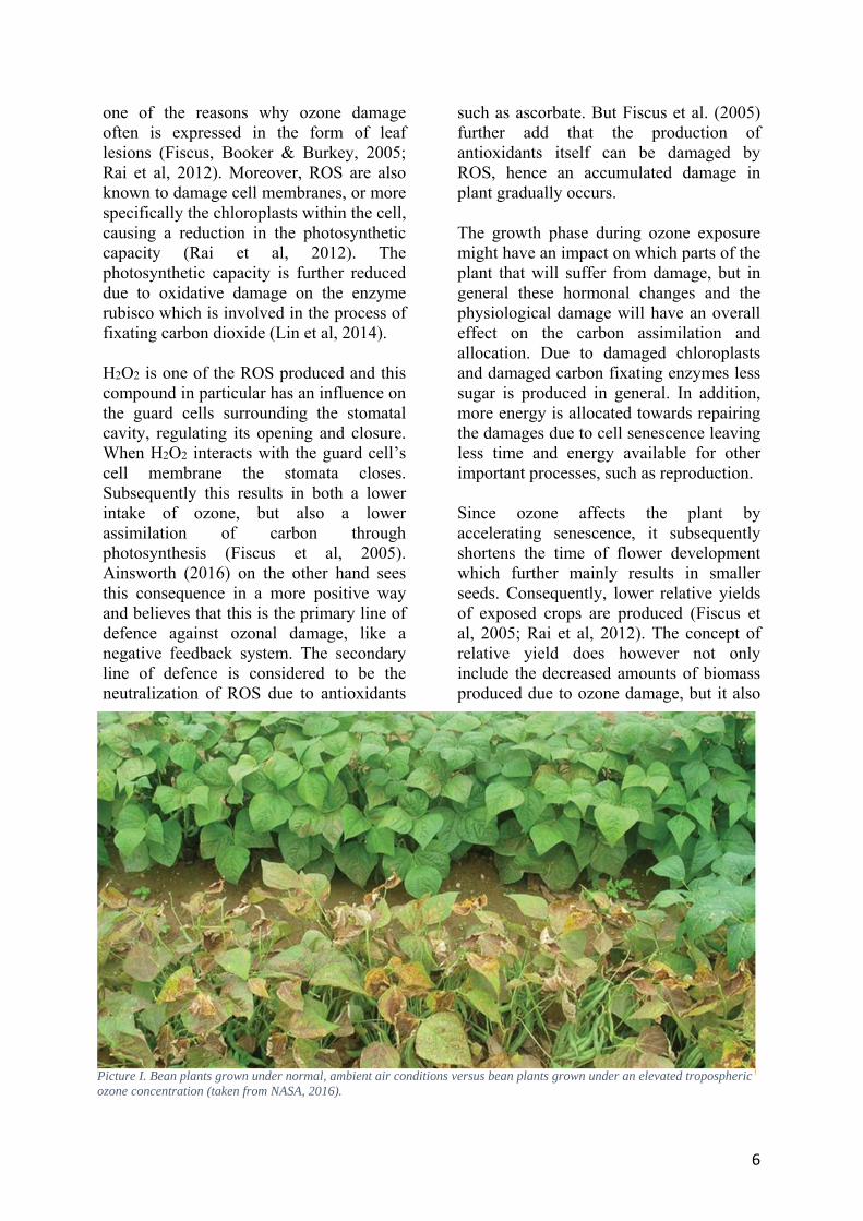
one of the reasons why ozone damage often is expressed in the form of leaf lesions (Fiscus, Booker & Burkey, 2005; Rai et al, 2012). Moreover, ROS are also known to damage cell membranes, or more specifically the chloroplasts within the cell, causing a reduction in the photosynthetic capacity (Rai et al, 2012). The photosynthetic capacity is further reduced due to oxidative damage on the enzyme rubisco which is involved in the process of fixating carbon dioxide (Lin et al, 2014). H2O2 is one of the ROS produced and this compound in particular has an influence on the guard cells surrounding the stomatal cavity, regulating its opening and closure. When H2O2 interacts with the guard cell’s cell membrane the stomata closes. Subsequently this results in both a lower intake of ozone, but also a lower assimilation of carbon through photosynthesis (Fiscus et al, 2005). Ainsworth (2016) on the other hand sees this consequence in a more positive way and believes that this is the primary line of defence against ozonal damage, like a negative feedback system. The secondary line of defence is considered to be the neutralization of ROS due to antioxidants

such as ascorbate. But Fiscus et al. (2005) further add that the production of antioxidants itself can be damaged by ROS, hence an accumulated damage in plant gradually occurs. The growth phase during ozone exposure might have an impact on which parts of the plant that will suffer from damage, but in general these hormonal changes and the physiological damage will have an overall effect on the carbon assimilation and allocation. Due to damaged chloroplasts and damaged carbon fixating enzymes less sugar is produced in general. In addition, more energy is allocated towards repairing the damages due to cell senescence leaving less time and energy available for other important processes, such as reproduction. Since ozone affects the plant by accelerating senescence, it subsequently shortens the time of flower development which further mainly results in smaller seeds. Consequently, lower relative yields of exposed crops are produced (Fiscus et al, 2005; Rai et al, 2012). The concept of relative yield does however not only include the decreased amounts of biomass produced due to ozone damage, but it also

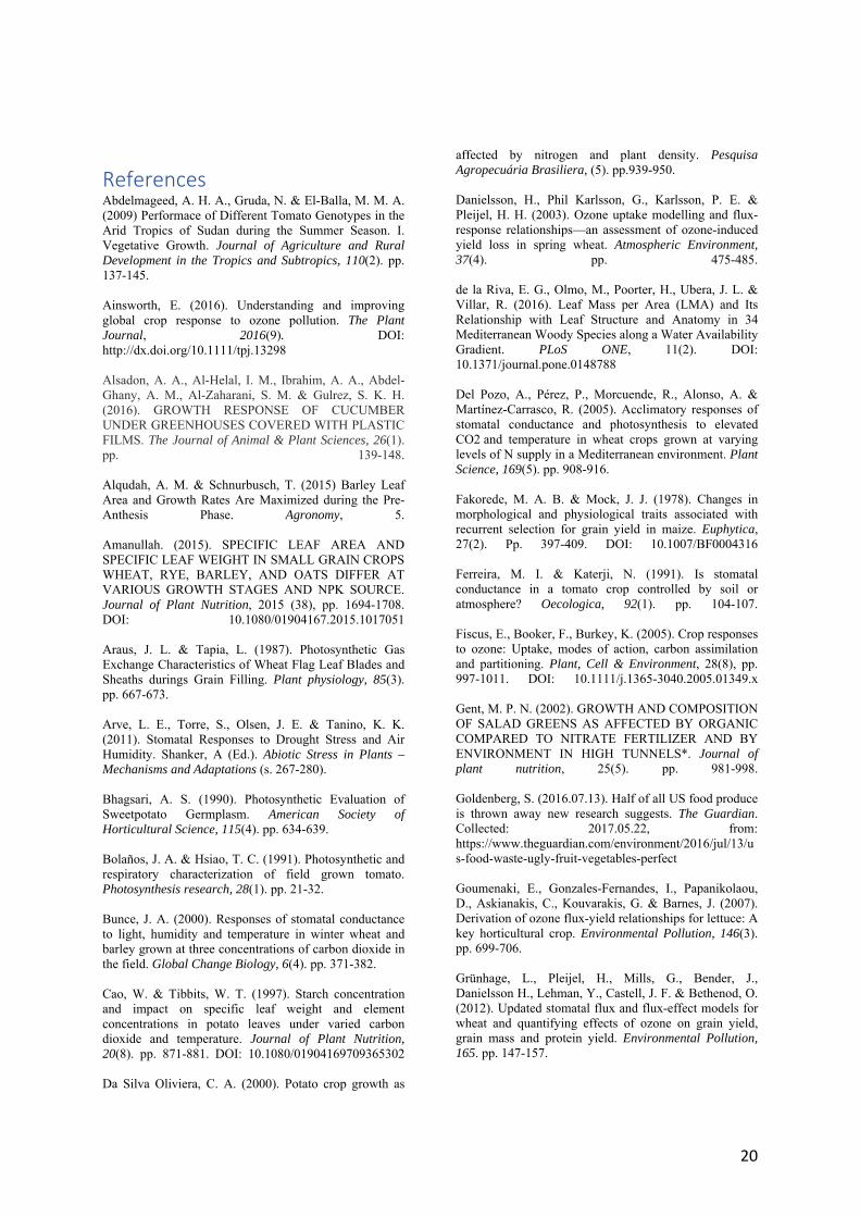
Picture I. Bean plants grown under normal, ambient air conditions versus bean plants grown under an elevated tropospheric ozone concentration (taken from NASA, 2016).

7

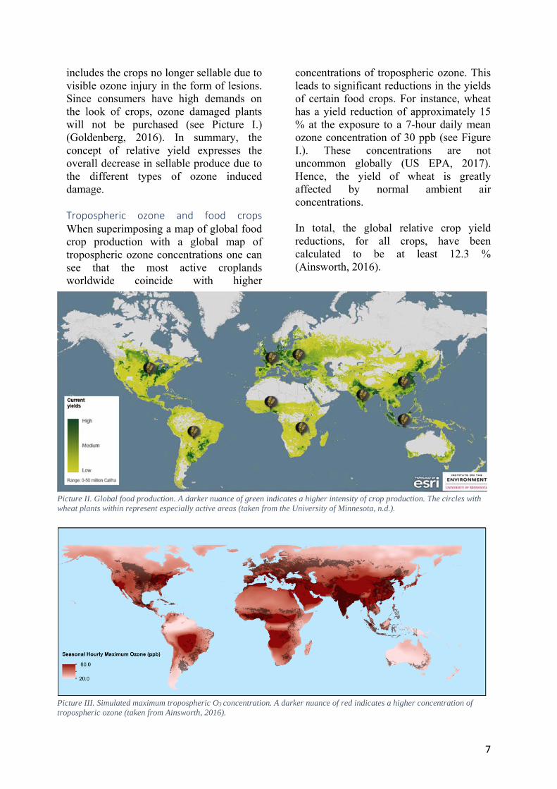
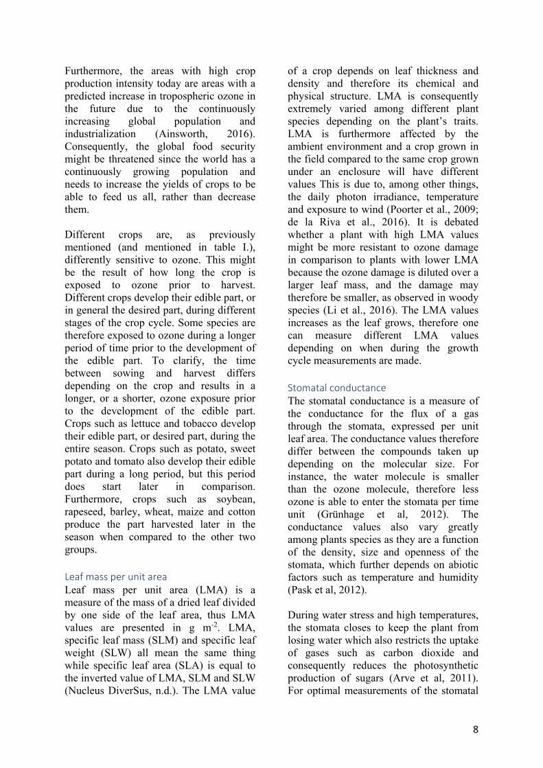
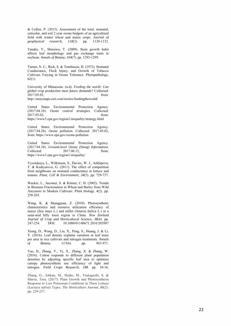
includes the crops no longer sellable due to visible ozone injury in the form of lesions. Since consumers have high demands on the look of crops, ozone damaged plants will not be purchased (see Picture I.) (Goldenberg, 2016). In summary, the concept of relative yield expresses the overall decrease in sellable produce due to the different types of ozone induced damage. Tropospheric ozone and food crops When superimposing a map of global food crop production with a global map of tropospheric ozone concentrations one can see that the most active croplands worldwide coincide with higher

concentrations of tropospheric ozone. This leads to significant reductions in the yields of certain food crops. For instance, wheat has a yield reduction of approximately 15 % at the exposure to a 7-hour daily mean ozone concentration of 30 ppb (see Figure I.). These concentrations are not uncommon globally (US EPA, 2017). Hence, the yield of wheat is greatly affected by normal ambient air concentrations. In total, the global relative crop yield reductions, for all crops, have been calculated to be at least 12.3 % (Ainsworth, 2016).

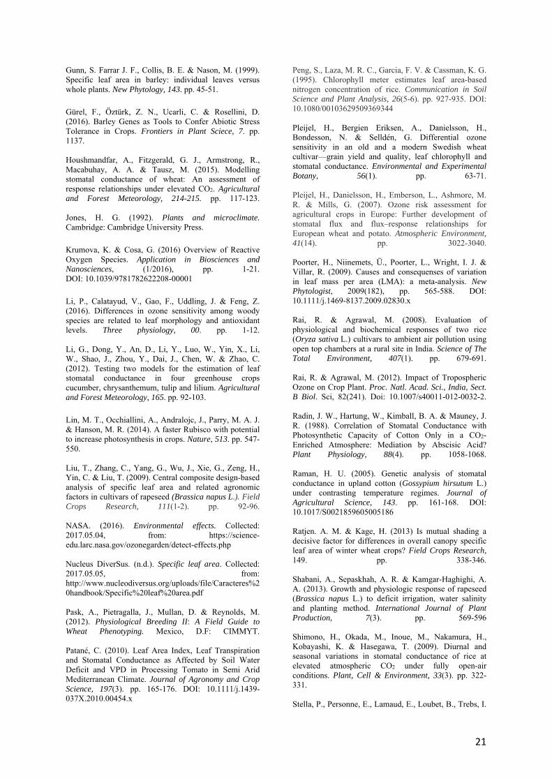
Picture II. Global food production. A darker nuance of green indicates a higher intensity of crop production. The circles with wheat plants within represent especially active areas (taken from the University of Minnesota, n.d.).

Picture III. Simulated maximum tropospheric O3 concentration. A darker nuance of red indicates a higher concentration of tropospheric ozone (taken from Ainsworth, 2016).

8

Furthermore, the areas with high crop production intensity today are areas with a predicted increase in tropospheric ozone in the future due to the continuously increasing global population and industrialization (Ainsworth, 2016). Consequently, the global food security might be threatened since the world has a continuously growing population and needs to increase the yields of crops to be able to feed us all, rather than decrease them. Different crops are, as previously mentioned (and mentioned in table I.), differently sensitive to ozone. This might be the result of how long the crop is exposed to ozone prior to harvest. Different crops develop their edible part, or in general the desired part, during different stages of the crop cycle. Some species are therefore exposed to ozone during a longer period of time prior to the development of the edible part. To clarify, the time between sowing and harvest differs depending on the crop and results in a longer, or a shorter, ozone exposure prior to the development of the edible part. Crops such as lettuce and tobacco develop their edible part, or desired part, during the entire season. Crops such as potato, sweet potato and tomato also develop their edible part during a long period, but this period does start later in comparison. Furthermore, crops such as soybean, rapeseed, barley, wheat, maize and cotton produce the part harvested later in the season when compared to the other two groups. Leaf mass per unit area Leaf mass per unit area (LMA) is a measure of the mass of a dried leaf divided by one side of the leaf area, thus LMA values are presented in g m-2. LMA, specific leaf mass (SLM) and specific leaf weight (SLW) all mean the same thing while specific leaf area (SLA) is equal to the inverted value of LMA, SLM and SLW (Nucleus DiverSus, n.d.). The LMA value

of a crop depends on leaf thickness and density and therefore its chemical and physical structure. LMA is consequently extremely varied among different plant species depending on the plant’s traits. LMA is furthermore affected by the ambient environment and a crop grown in the field compared to the same crop grown under an enclosure will have different values This is due to, among other things, the daily photon irradiance, temperature and exposure to wind (Poorter et al., 2009; de la Riva et al., 2016). It is debated whether a plant with high LMA values might be more resistant to ozone damage in comparison to plants with lower LMA because the ozone damage is diluted over a larger leaf mass, and the damage may therefore be smaller, as observed in woody species (Li et al., 2016). The LMA values increases as the leaf grows, therefore one can measure different LMA values depending on when during the growth cycle measurements are made. Stomatal conductance The stomatal conductance is a measure of the conductance for the flux of a gas through the stomata, expressed per unit leaf area. The conductance values therefore differ between the compounds taken up depending on the molecular size. For instance, the water molecule is smaller than the ozone molecule, therefore less ozone is able to enter the stomata per time unit (Grünhage et al, 2012). The conductance values also vary greatly among plants species as they are a function of the density, size and openness of the stomata, which further depends on abiotic factors such as temperature and humidity (Pask et al, 2012). During water stress and high temperatures, the stomata closes to keep the plant from losing water which also restricts the uptake of gases such as carbon dioxide and consequently reduces the photosynthetic production of sugars (Arve et al, 2011). For optimal measurements of the stomatal

9

conductance, the leaf should be exposed to sunny conditions while avoiding water stress. The measurements should further also preferably be taken before noon (Pask etaal,a2012).

Aim Different types of crops are more or less sensitive to ozone exposure and there are many theories as to why there is such variation in sensitivity. Therefore, the aim of this study is to analyse the relationship between ozone sensitivity in various crops and stomatal conductance, LMA and plant type.

Research questions • Is ozone sensitivity related to

stomatal conductance? • Is ozone sensitivity related to

LMA? • Are crop species which produce

their harvested part later in the growing season more sensitive to ozone damage, in comparison to crops producing their edible, or otherwise sought, parts earlier?

Method The data used to evaluate the relationship between LMA, stomatal conductance and ozone was found through an extensive search on various search engines such as Göteborgs Universitetsbibliotek: Supersök, Scopus, Google Scholar and regular Google. The same search engines were furthermore also used to find basic articles on the formation of tropospheric ozone, LMA and stomatal conductance. Supervisor Johan Uddling also provided me with specific articles regarding previous research and other relevant information on the topic. The main words used when searching for data from the various article search engines: specific leaf area, SLA, specific leaf weight, specific leaf mass, leaf mass per unit area, LMA, stomatal conductance,

ozone. These search words were used in combination with the name of the different crop species in both Latin and English to find articles with relevant data. This study covers 13 species of crops: potato, tomato, cotton, lettuce, rapeseed, tobacco, wheat, barley, maize, sweet potato, soybean, rice and cucumber. These species were specifically selected based on a few criteria. Primarily, the amount of data in the ozone sensitivity database provided by Gina Mills (Table I., Appendix) narrowed down the selection. Most of the species used had a lot of data to base their ozone sensitivity on, but a few species’ sensitivity was based on fewer data points. For instance, cucumber and rapeseed. These crops were anyhow used in the study because many of these few data points were mean averages from different studies based on larger amounts data. In this study, the ozone sensitivity was correlated to both stomatal conductance and LMA. Thus, both stomatal conductance and LMA values were needed for all species. This further restricted the selection since these values were not found for all species with sufficient ozone sensitivity data. As mentioned above the ozone sensitivity was collected from a database. This database established the sensitivity value of each crop based on previously carried out research (see Figure I.). Hence, some crops had more material to base the sensitivity on than other depending on how well studied the crop’s ozone vulnerability was. Certain crops are naturally cultivated in the field while others are grown in greenhouses. Therefore, some crops sensitivity data were based on studies conducted during field conditions grown in soil while other crops where raised in glasshouses and pots, for instance tomato,

10

lettuce and cucumber. For the ozone sensitivity value to be correlatable to values of stomatal conductance and LMA it was therefore necessary to try and match how the different studies, from where the data was collected from, were carried out. If for instance the ozone sensitivity data was deduced from field studies, the studies from where the stomatal conductance and LMA values where taken should also be conducted in the field. In some species, this criterion could however not be fulfilled since studies conducted in the same matter were not found for all variables. Hence, some data points might therefore not be usable in a regression analysis. The LMA values used had to furthermore be values taken from mature or newly fully expanded leafs. The stomatal conductance values where ones collected during morning hours during cloudless conditions. The values found for both stomatal conductance and LMA were not all presented in the same units. The values were therefore either directly collected from the articles or first recalculated, for all the values to be comparable to each other. The comparable unit used for stomatal conductance was mmole O3 m-2 s-

1 while the comparable unit used for LMA was g m-2.

Stomatal conductance calculations The data collected were mainly expressed in the unit mmole m-2 s-1, but the values were often also given in mole m-2 s-1 or cm s-1. Moreover, the stomatal conductance given was often expressed as the conductance of water. Thus, a conversion was made by multiplying the water conductance value with 0.663 to recalculate it into the ozone conductance (Grünhage et al, 2012). 25 mole m-2 s-1 = 0.25 mmole m-2 s-1

To convert a value from mm/s to mole/m2/s you multiply the mm/s-value with 0.04 (Jones, 1992). 25 mm s-1 = 25*0.04 mole m-2 s-1 = 1 mole m-2 s-1 → mmole m-2 s-1 → 0.001 mmole m-2 s-1 LMA calculations The LMA data collected were mainly data expressed in the unit g m-2. Data on specific leaf mass (SLA), the inverse of LMA, were either expressed in the unit cm2 mg-1 or cm2 g-1 and were recalculated into the common unit g m-2. 25 cm2 mg-1 = 0.0025 m2 mg-1 → . mg m-2 → 400 mg m-2 → g m-2 = 0.4 g m-2 25 cm2 g-1 = 0.0025 m2 g-1 → . g m-2 → 400 g m-2 Some LMA data were given in the units mg/mm2 or mg/cm2 and were also recalculated into the common unit g/m2.

0.25 mg mm-2 = 0.00025 g mm-2 → 0.00025*1000*1000 g m-2 → 250 g m-2 0.25 mg cm-2 = 0.00025 g cm-2 → 0.00025*100*100 g m-2 → 2.5 g m-2

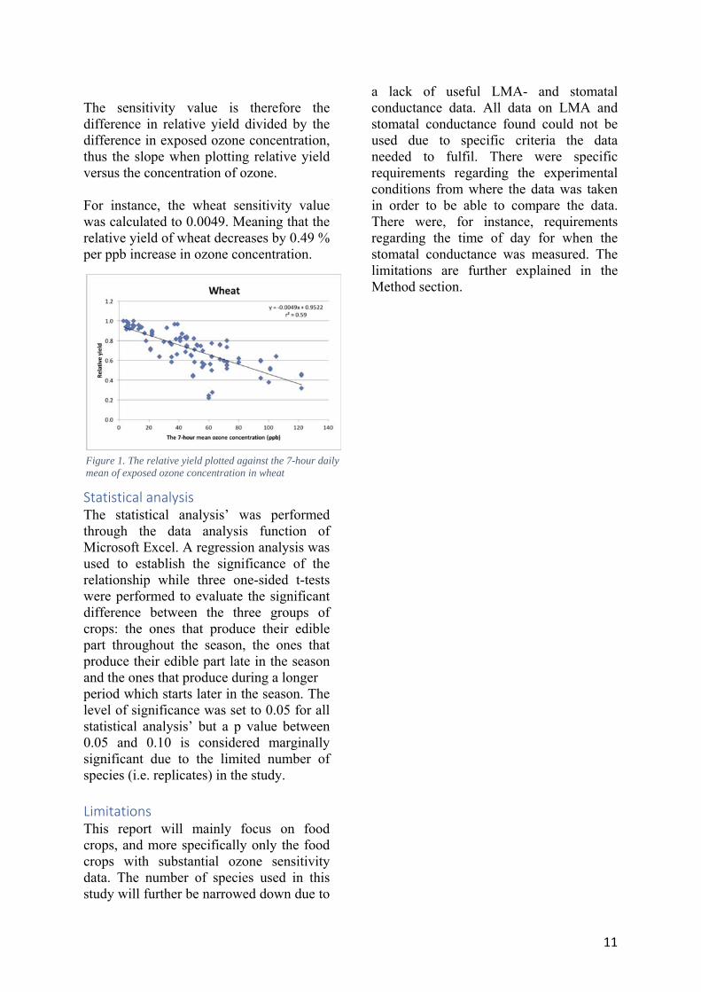
Establishing ozone sensitivity The ozone sensitivity value used in this review was, as previously mentioned, derived by Gina Mills from many studies where the relative yield decrease of the crop is dependent on the different concentrations of ozone exposure (see appendix for references). The crops were exposed for seven hours, either between 10:00-17:00 or 09:00-16:00, and the 7-hour mean average concentration was then used in the regression (see Figure I.).

11

The sensitivity value is therefore the difference in relative yield divided by the difference in exposed ozone concentration, thus the slope when plotting relative yield versus the concentration of ozone. For instance, the wheat sensitivity value was calculated to 0.0049. Meaning that the relative yield of wheat decreases by 0.49 % per ppb increase in ozone concentration.

Statistical analysis The statistical analysis’ was performed through the data analysis function of Microsoft Excel. A regression analysis was used to establish the significance of the relationship while three one-sided t-tests were performed to evaluate the significant difference between the three groups of crops: the ones that produce their edible part throughout the season, the ones that produce their edible part late in the season and the ones that produce during a longer period which starts later in the season. The level of significance was set to 0.05 for all statistical analysis’ but a p value between 0.05 and 0.10 is considered marginally significant due to the limited number of species (i.e. replicates) in the study.

Limitations This report will mainly focus on food crops, and more specifically only the food crops with substantial ozone sensitivity data. The number of species used in this study will further be narrowed down due to

a lack of useful LMA- and stomatal conductance data. All data on LMA and stomatal conductance found could not be used due to specific criteria the data needed to fulfil. There were specific requirements regarding the experimental conditions from where the data was taken in order to be able to compare the data. There were, for instance, requirements regarding the time of day for when the stomatal conductance was measured. The limitations are further explained in the Method section.

Figure 1. The relative yield plotted against the 7-hour daily mean of exposed ozone concentration in wheat

12

12

Tables Table I. The table below summarizes the raw data from the ozone sensitivity data base. Crop species Ozone sensitivity (yield reductions per ppb of ozone)

Number of data points Significance of slope (p-values) At which [O3] is there significant yield reduction? Relative yield at 60 ppb of ozone Potato 0.00197 70 0.066 29 ppb 0.814 Sweet potato 0.00173 6 0.118 59 ppb 0.556 Soybean 0.00505 50 < 0.001 8 ppb 0.703 Rice 0.00386 145 < 0.001 11 ppb 0.823 Tomato 0.00386 41 0.004 27 ppb 0.78 Cucumber 0.00185 4 0.049 48 ppb 0.89 Lettuce 0.00653 26 0.035 43 ppb 0.819 Rapeseed 0.00311 29 0.004 25 ppb 0.752 Barley 0.00198 59 0.038 43 ppb 0.866 Wheat 0.00491 93 < 0.001 9 ppb 0.658 Maize 0.00311 23 < 0.001 25 ppb 0.843 Cotton 0.00722 17 Information is missing Information is missing 0.729 Tobacco 0.00346 6 Information is missing Information is missing 0.928

13

Table II. The table below lists the collected stomatal conductance values as well as the timing of when the edible, or otherwise sought, part is produced during the season. The values are either directly collected from a single study or an average of different studies. Crop species Stomatal conductance (mmole m-2 s-1) Growth conditions When is the harvested part produced? Reference Potato 750 Filed grown under open top chambers During a longer period, which starts earlier Pleijel et al, (2007) Sweet potato 276 Field grown, partly under a plastic cover During a longer period, which starts earlier Bhagasari, (1990) Soybean 366 No information available Late in the season Tanaka & Shiraiwa, (2009) Tomato 281 Field grown and in pots in a greenhouse During a longer period, which starts earlier Ferreira & Katerji, (1992); Vysotskaya et al., (2011); Bolaños & Hsiao, (1991); Patané., (2010) Cucumber 480 Grown in a greenhouse During the entire season Li et al., (2012) Lettuce 171 Field grown and in pots in greenhouse During the entire season Zhang et al., (2016); Vsotskaya et al., (2011); Goumenaki et al., (2007) Rapeseed 126 Field grown Late in the season Shabani et al., (2013) Barley 431 Field grown under open top chambers Late in the season Bunce., (2000) Wheat 351 Field grown without enclosures and under open top chambers Late in the season Stella et al, (2013); Araus & Tapia, (1987); Pleijel et al, (2006); Del Pozo, (2005); Houshmandfar et al, (2015); Bunce, (2000) Maize 184 Field grown Late in the season Stella et al., (2013); Wang & Shangguan, (2010) Cotton 711 Field grown under open top chambers Late in the season Rahman., (2005); Radin et al., (1998) Tobacco 141 Field grown During the entire season Turner et al., (1971) Rice 260 Field grown Late in the season Shimono et al., (2009)

14

Table III. The table below lists the collected LMA values as well as the timing of when the edible, or otherwise sought, part is produced during the season. The values are either directly collected from a single study or an average of different studies. Crop species LMA (g m-2) Growth conditions When is the harvested part produced? Reference Potato 40.4 No information available in one of the studies, in pots in the other study During a longer period, which starts earlier Cao & Tibbits, (1997); Da Silva, (1999) Soybean 50 No information available Late in the season Tanaka & Shiraiwa, (2009) Rice 52.2 Field grown in soil and in pots Late in the season Peng et al, (2008); Huang et al, (2015) Tomato 95.3 Field grown During a longer period, which starts earlier Abdelmageed et al, (2009) Cucumber 33.9 Field grown under a plastic cover During the entire season Alsadon, et al, (2016) Lettuce 26.9 Pots in a greenhouse and grown under an enclosure in the form of tunnels During the entire season Zhang et al, (2016); Gent, (2002) Rapeseed 123.4 Field grown Late in the season Liu et al, (2009) Barley 33 Pots and trays outdoors Late in the season Gunn et al, (1999); Wacker et al, (2002) Wheat 35.8 Pots in a greenhouse and field grown partly carried out under a rain-out-shelter Late in the season Amanullah, (2015); Ratjen & Kage, (2012) Maize 58.8 Field grown Late in the season Fakorede & Mock, (1979); Wang & Shangguan, (2010) Cotton 71.9 Field grown, partly under a plastic cover Late in the season Yao et al, (2016)

15

Results The figures below display the relationship between ozone sensitivity and stomatal conductance, ozone sensitivity and LMA as well as ozone sensitivity and the ratio of stomatal conductance to LMA. The caption below each figure states the R2-value and the p-value of the relationship. Figure V. and VI. present the ozone sensitivity of the 13 different crops and if the crop produces its harvested part during the whole season (WS), during a longer period which starts late (DLP) or late in the growing season (LIS). Figure VI. further displays the difference between LIS- and DLP-crops.

.

There was no statistically significant relationship between neither ozone sensitivity and stomatal conductance nor ozone sensitivity and LMA (Figure II. and Figure III.). Figure IV. displays the relationship between ozone sensitivity and the ratio of stomatal conductance to LMA. This variable is studied, beyond simply studying the relationship between ozone sensitivity and LMA respective stomatal conductance, because it regards both LMA and stomatal conductance. Consequently, this quota implies the conductance of gas inlet per mass of leaf. However, no statistical significance was found (p = 0.44) for this relationship either but the p-value was lower in comparison to the other relationships. If significant, this relationship would indicate that a higher quota of the ratio of stomatal conductance to indicates a lower ozone sensitivity while a lower quota indicates a higher sensitivity.

Figure II. The ozone sensitivity of each crop plotted against the crop’s stomatal conductance. The R2-value was calculated to 0.003 while the p-value was 0.86.

Figure IV. The ozone sensitivity plotted against the uptake of ozone in mmole per seconds per gram. The R2-value was calculated to 0.067 while the p-value was 0.44

Figure III. The ozone sensitivity of each crop plotted against the crops LMA-value. The R2-value was calculated to 0.001 while the p-value was 0.93.

16

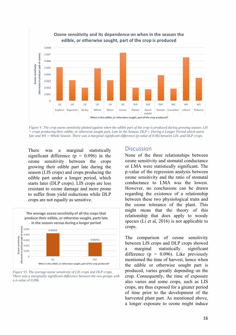
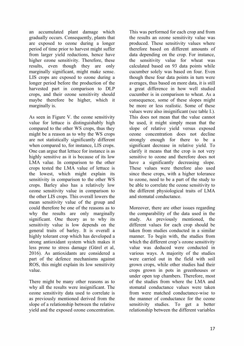
There was a marginal statistically significant difference (p = 0.096) in the ozone sensitivity between the crops growing their edible part late during the season (LIS crops) and crops producing the edible part under a longer period, which starts later (DLP crops). LIS crops are less resistant to ozone damage and more prone to suffer from yield reductions while DLP crops are not equally as sensitive.

Discussion None of the three relationships between ozone sensitivity and stomatal conductance or LMA were statistically significant. The p-value of the regression analysis between ozone sensitivity and the ratio of stomatal conductance to LMA was the lowest. However, no conclusions can be drawn regarding the existence of a relationship between these two physiological traits and the ozone tolerance of the plant. This might mean that the theory of this relationship that does apply to woody species (Li et al, 2016) is not applicable to crops. The comparison of ozone sensitivity between LIS crops and DLP crops showed a marginal statistically significant difference (p = 0.096). Like previously mentioned the time of harvest, hence when the edible or otherwise sought part is produced, varies greatly depending on the crop. Consequently, the time of exposure also varies and some crops, such as LIS crops, are thus exposed for a greater period of time prior to the development of the harvested plant part. As mentioned above, a longer exposure to ozone might induce

Figure V. The crop ozone sensitivity plotted against when the edible part of the crop is produced during growing season. LIS = crops producing their edible, or otherwise sought part, Late In the Season, DLP = During a Longer Period which starts late and WS = Whole Season. There was a marginal significant difference (p-value of 0.06) between LIS- and DLP crops.

Figure VI. The average ozone sensitivity of LIS crops and DLP crops. There was a marginally significant difference between the two groups with a p-value of 0.096.

17

an accumulated plant damage which gradually occurs. Consequently, plants that are exposed to ozone during a longer period of time prior to harvest might suffer from larger yield reductions, hence have higher ozone sensitivity. Therefore, these results, even though they are only marginally significant, might make sense. LIS crops are exposed to ozone during a longer period before the production of the harvested part in comparison to DLP crops, and their ozone sensitivity should maybe therefore be higher, which it marginally is. As seen in Figure V. the ozone sensitivity value for lettuce is distinguishably high compared to the other WS crops, thus they might be a reason as to why the WS crops are not statistically significantly different when compared to, for instance, LIS crops. One can argue that lettuce for instance is as highly sensitive as it is because of its low LMA value. In comparison to the other crops tested the LMA value of lettuce is the lowest, which might explain its sensitivity in comparison to the other WS crops. Barley also has a relatively low ozone sensitivity value in comparison to the other LIS crops. This overall lowers the mean sensitivity value of the group and could therefore be one of the reasons as to why the results are only marginally significant. One theory as to why its sensitivity value is low depends on the general traits of barley. It is overall a highly tolerant crop which has developed a strong antioxidant system which makes it less prone to stress damage (Gürel et al, 2016). As antioxidants are considered a part of the defence mechanisms against ROS, this might explain its low sensitivity value. There might be many other reasons as to why all the results were insignificant. The ozone sensitivity data used to correlate is as previously mentioned derived from the slope of a relationship between the relative yield and the exposed ozone concentration.

This was performed for each crop and from the results an ozone sensitivity value was produced. These sensitivity values where therefore based on different amounts of data depending on the crop. For instance, the sensitivity value for wheat was calculated based on 93 data points while cucumber solely was based on four. Even though these four data points in turn were averages, thus based on more data, it is still a great difference in how well studied cucumber is in comparison to wheat. As a consequence, some of these slopes might be more or less realistic. Some of these values were also insignificant (see table I.). This does not mean that the value cannot be used, it might simply mean that the slope of relative yield versus exposed ozone concentration does not decline strongly enough for there to be a significant decrease in relative yield. To clarify it means that the crop is not very sensitive to ozone and therefore does not have a significantly decreasing slope. These values were therefore also used since these crops, with a higher tolerance to ozone, need to be a part of the study to be able to correlate the ozone sensitivity to the different physiological traits of LMA and stomatal conductance. Moreover, there are other issues regarding the comparability of the data used in the study. As previously mentioned, the different values for each crop should be taken from studies conducted in a similar manner. To begin with, the studies from which the different crop’s ozone sensitivity value was deduced were conducted in various ways. A majority of the studies were carried out in the field with soil grown crops, while other studies had their crops grown in pots in greenhouses or under open top chambers. Therefore, most of the studies from where the LMA and stomatal conductance values were taken from were matched conductance-wise to the manner of conductance for the ozone sensitivity studies. To get a better relationship between the different variables

18

the conductance of the studies used should match though, which was not achieved due to the lack of data fulfilling the other, more important, criterion. The reason why the studies should be conducted in the same manner is due to the fact that there are certain factors which influence LMA and stomatal conductance. For instance, daily photon irradiance, temperature, humidity or exposure to wind. Consequently, a study carried out in a greenhouse might not be comparable to a field study due these abiotic factors being different. In addition, LMA values vary greatly depending on when the measurement is carried out during the plant cycle and all LMA values used in this study are not from the same plant phase, which results in the values not being comparable. The same line of reasoning could be applied to the stomatal conductance data as well. Stomatal conductance varies with temperature, and the leaf temperature was not even mentioned in the majority of the studies from where the data was collected from. Hence, this could also be a source of error. Furthermore, another reason as to why none of the results were significant might be due to the relatively few number of species included. Due to the criteria of the studies mentioned above only a few values for LMA and stomatal conductance were found and used. More data might give a stronger correlation (R2-value), thus smaller p-value. If more research was conducted on this topic, and more studies on LMA and stomatal conductance were carried out there would be more usable data available and more conclusions could be drawn regarding the various ozone sensitivity among crops. As many of the places of large food production globally also are some of the most ozone exposed areas, it is evident that

this pollutant has a large impact on crop yields. Not only due to a lower yield but also due to crops being rejected and considered second quality because of the lesions sometimes caused on leaves due to the exposure. Overall, this leads to reduced amounts of food produced and sold, resulting in many problems. Lower yield produced is mainly the largest issue since less food means less people being able to eat. But since the amounts of sellable crops might be further reduced due to ugly looks it is also a financial problem for the farmers making a living on selling produce. With this said, the result of this study might be able to indicate which crops are more suitable for production in these types of areas. Preferably crops that produce their edible, or otherwise sought, parts earlier in the season would be to recommend.

Conclusions Overall this study indicates that crops that produce their edible, or otherwise sought, parts earlier in the season are less prone to reduced yields due to ozone damage in comparison to crops producing their harvested parts later in the growing season. These results coincide with the claim that ozone damage accumulates and that crops producing the parts harvested late in the season will have been exposed to ozone longer prior to this. There was not a statistically significant relationship between either ozone sensitivity and stomatal conductance nor ozone sensitivity and LMA. No statistically significant results were either derived when combining these two physiological traits and studying the relationship between ozone sensitivity and the ratio of stomatal conductance to LMA. This might indicate that there is not a relationship between these physiological traits and ozone sensitivity, but this conclusion should only be drawn from a study with more and better data.

19

Acknowledgements I would first and foremost like to thank my supervisor Johan Uddling Fredin for giving me the opportunity to work with a subject I am truly interested in, as well as giving me both advice and help when needed. I would also like to thank my friends and family who gave me support and feedback throughout the project.

20

References Abdelmageed, A. H. A., Gruda, N. & El-Balla, M. M. A. (2009) Performace of Different Tomato Genotypes in the Arid Tropics of Sudan during the Summer Season. I. Vegetative Growth. Journal of Agriculture and Rural Development in the Tropics and Subtropics, 110(2). pp. 137-145. Ainsworth, E. (2016). Understanding and improving global crop response to ozone pollution. The Plant Journal, 2016(9). DOI: http://dx.doi.org/10.1111/tpj.13298 Alsadon, A. A., Al-Helal, I. M., Ibrahim, A. A., Abdel-Ghany, A. M., Al-Zaharani, S. M. & Gulrez, S. K. H. (2016). GROWTH RESPONSE OF CUCUMBER UNDER GREENHOUSES COVERED WITH PLASTIC FILMS. The Journal of Animal & Plant Sciences, 26(1). pp. 139-148. Alqudah, A. M. & Schnurbusch, T. (2015) Barley Leaf Area and Growth Rates Are Maximized during the Pre-Anthesis Phase. Agronomy, 5. Amanullah. (2015). SPECIFIC LEAF AREA AND SPECIFIC LEAF WEIGHT IN SMALL GRAIN CROPS WHEAT, RYE, BARLEY, AND OATS DIFFER AT VARIOUS GROWTH STAGES AND NPK SOURCE. Journal of Plant Nutrition, 2015 (38), pp. 1694-1708. DOI: 10.1080/01904167.2015.1017051 Araus, J. L. & Tapia, L. (1987). Photosynthetic Gas Exchange Characteristics of Wheat Flag Leaf Blades and Sheaths durings Grain Filling. Plant physiology, 85(3). pp. 667-673. Arve, L. E., Torre, S., Olsen, J. E. & Tanino, K. K. (2011). Stomatal Responses to Drought Stress and Air Humidity. Shanker, A (Ed.). Abiotic Stress in Plants – Mechanisms and Adaptations (s. 267-280). Bhagsari, A. S. (1990). Photosynthetic Evaluation of Sweetpotato Germplasm. American Society of Horticultural Science, 115(4). pp. 634-639. Bolaños, J. A. & Hsiao, T. C. (1991). Photosynthetic and respiratory characterization of field grown tomato. Photosynthesis research, 28(1). pp. 21-32. Bunce, J. A. (2000). Responses of stomatal conductance to light, humidity and temperature in winter wheat and barley grown at three concentrations of carbon dioxide in the field. Global Change Biology, 6(4). pp. 371-382. Cao, W. & Tibbits, W. T. (1997). Starch concentration and impact on specific leaf weight and element concentrations in potato leaves under varied carbon dioxide and temperature. Journal of Plant Nutrition, 20(8). pp. 871-881. DOI: 10.1080/01904169709365302 Da Silva Oliviera, C. A. (2000). Potato crop growth as

affected by nitrogen and plant density. Pesquisa Agropecuária Brasiliera, (5). pp.939-950. Danielsson, H., Phil Karlsson, G., Karlsson, P. E. & Pleijel, H. H. (2003). Ozone uptake modelling and flux-response relationships—an assessment of ozone-induced yield loss in spring wheat. Atmospheric Environment, 37(4). pp. 475-485. de la Riva, E. G., Olmo, M., Poorter, H., Ubera, J. L. & Villar, R. (2016). Leaf Mass per Area (LMA) and Its Relationship with Leaf Structure and Anatomy in 34 Mediterranean Woody Species along a Water Availability Gradient. PLoS ONE, 11(2). DOI: 10.1371/journal.pone.0148788 Del Pozo, A., Pérez, P., Morcuende, R., Alonso, A. & Martínez-Carrasco, R. (2005). Acclimatory responses of stomatal conductance and photosynthesis to elevated CO2 and temperature in wheat crops grown at varying levels of N supply in a Mediterranean environment. Plant Science, 169(5). pp. 908-916. Fakorede, M. A. B. & Mock, J. J. (1978). Changes in morphological and physiological traits associated with recurrent selection for grain yield in maize. Euphytica, 27(2). Pp. 397-409. DOI: 10.1007/BF0004316 Ferreira, M. I. & Katerji, N. (1991). Is stomatal conductance in a tomato crop controlled by soil or atmosphere? Oecologica, 92(1). pp. 104-107. Fiscus, E., Booker, F., Burkey, K. (2005). Crop responses to ozone: Uptake, modes of action, carbon assimilation and partitioning. Plant, Cell & Environment, 28(8), pp. 997-1011. DOI: 10.1111/j.1365-3040.2005.01349.x Gent, M. P. N. (2002). GROWTH AND COMPOSITION OF SALAD GREENS AS AFFECTED BY ORGANIC COMPARED TO NITRATE FERTILIZER AND BY ENVIRONMENT IN HIGH TUNNELS*. Journal of plant nutrition, 25(5). pp. 981-998. Goldenberg, S. (2016.07.13). Half of all US food produce is thrown away new research suggests. The Guardian. Collected: 2017.05.22, from: https://www.theguardian.com/environment/2016/jul/13/us-food-waste-ugly-fruit-vegetables-perfect Goumenaki, E., Gonzales-Fernandes, I., Papanikolaou, D., Askianakis, C., Kouvarakis, G. & Barnes, J. (2007). Derivation of ozone flux-yield relationships for lettuce: A key horticultural crop. Environmental Pollution, 146(3). pp. 699-706. Grünhage, L., Pleijel, H., Mills, G., Bender, J., Danielsson H., Lehman, Y., Castell, J. F. & Bethenod, O. (2012). Updated stomatal flux and flux-effect models for wheat and quantifying effects of ozone on grain yield, grain mass and protein yield. Environmental Pollution, 165. pp. 147-157.

21

Gunn, S. Farrar J. F., Collis, B. E. & Nason, M. (1999). Specific leaf area in barley: individual leaves versus whole plants. New Phytology, 143. pp. 45-51.

Gürel, F., Öztürk, Z. N., Ucarli, C. & Rosellini, D. (2016). Barley Genes as Tools to Confer Abiotic Stress Tolerance in Crops. Frontiers in Plant Sciece, 7. pp. 1137. Houshmandfar, A., Fitzgerald, G. J., Armstrong, R., Macabuhay, A. A. & Tausz, M. (2015). Modelling stomatal conductance of wheat: An assessment of response relationships under elevated CO2. Agricultural and Forest Meteorology, 214-215. pp. 117-123. Jones, H. G. (1992). Plants and microclimate. Cambridge: Cambridge University Press.

Krumova, K. & Cosa, G. (2016) Overview of Reactive Oxygen Species. Application in Biosciences and Nanosciences, (1/2016), pp. 1-21. DOI: 10.1039/9781782622208-00001

Li, P., Calatayud, V., Gao, F., Uddling, J. & Feng, Z. (2016). Differences in ozone sensitivity among woody species are related to leaf morphology and antioxidant levels. Three physiology, 00. pp. 1-12. Li, G., Dong, Y., An, D., Li, Y., Luo, W., Yin, X., Li, W., Shao, J., Zhou, Y., Dai, J., Chen, W. & Zhao, C. (2012). Testing two models for the estimation of leaf stomatal conductance in four greenhouse crops cucumber, chrysanthemum, tulip and lilium. Agricultural and Forest Meteorology, 165. pp. 92-103.

Lin, M. T., Occhiallini, A., Andralojc, J., Parry, M. A. J. & Hanson, M. R. (2014). A faster Rubisco with potential to increase photosynthesis in crops. Nature, 513. pp. 547-550. Liu, T., Zhang, C., Yang, G., Wu, J., Xie, G., Zeng, H., Yin, C. & Liu, T. (2009). Central composite design-based analysis of specific leaf area and related agronomic factors in cultivars of rapeseed (Brassica napus L.). Field Crops Research, 111(1-2). pp. 92-96. NASA. (2016). Environmental effects. Collected: 2017.05.04, from: https://science-edu.larc.nasa.gov/ozonegarden/detect-effects.php Nucleus DiverSus. (n.d.). Specific leaf area. Collected: 2017.05.05, from: http://www.nucleodiversus.org/uploads/file/Caracteres%20handbook/Specific%20leaf%20area.pdf Pask, A., Pietragalla, J., Mullan, D. & Reynolds, M. (2012). Physiological Breeding II: A Field Guide to Wheat Phenotyping. Mexico, D.F: CIMMYT. Patané, C. (2010). Leaf Area Index, Leaf Transpiration and Stomatal Conductance as Affected by Soil Water Deficit and VPD in Processing Tomato in Semi Arid Mediterranean Climate. Journal of Agronomy and Crop Science, 197(3). pp. 165-176. DOI: 10.1111/j.1439-037X.2010.00454.x

Peng, S., Laza, M. R. C., Garcia, F. V. & Cassman, K. G. (1995). Chlorophyll meter estimates leaf area-based nitrogen concentration of rice. Communication in Soil Science and Plant Analysis, 26(5-6). pp. 927-935. DOI: 10.1080/00103629509369344 Pleijel, H., Bergien Eriksen, A., Danielsson, H., Bondesson, N. & Selldén, G. Differential ozone sensitivity in an old and a modern Swedish wheat cultivar—grain yield and quality, leaf chlorophyll and stomatal conductance. Environmental and Experimental Botany, 56(1). pp. 63-71. Pleijel, H., Danielsson, H., Emberson, L., Ashmore, M. R. & Mills, G. (2007). Ozone risk assessment for agricultural crops in Europe: Further development of stomatal flux and flux–response relationships for European wheat and potato. Atmospheric Environment, 41(14). pp. 3022-3040. Poorter, H., Niinemets, Ü., Poorter, L., Wright, I. J. & Villar, R. (2009). Causes and consequenses of variation in leaf mass per area (LMA): a meta-analysis. New Phytologist, 2009(182), pp. 565-588. DOI: 10.1111/j.1469-8137.2009.02830.x Rai, R. & Agrawal, M. (2008). Evaluation of physiological and biochemical responses of two rice (Oryza sativa L.) cultivars to ambient air pollution using open top chambers at a rural site in India. Science of The Total Environment, 407(1). pp. 679-691. Rai, R. & Agrawal, M. (2012). Impact of Tropospheric Ozone on Crop Plant. Proc. Natl. Acad. Sci., India, Sect. B Biol. Sci, 82(241). Doi: 10.1007/s40011-012-0032-2. Radin, J. W., Hartung, W., Kimball, B. A. & Mauney, J. R. (1988). Correlation of Stomatal Conductance with Photosynthetic Capacity of Cotton Only in a CO2-Enriched Atmosphere: Mediation by Abscisic Acid? Plant Physiology, 88(4). pp. 1058-1068. Raman, H. U. (2005). Genetic analysis of stomatal conductance in upland cotton (Gossypium hirsutum L.) under contrasting temperature regimes. Journal of Agricultural Science, 143. pp. 161-168. DOI: 10.1017/S0021859605005186 Ratjen. A. M. & Kage, H. (2013) Is mutual shading a decisive factor for differences in overall canopy specific leaf area of winter wheat crops? Field Crops Research, 149. pp. 338-346. Shabani, A., Sepaskhah, A. R. & Kamgar-Haghighi, A. A. (2013). Growth and physiologic response of rapeseed (Brassica napus L.) to deficit irrigation, water salinity and planting method. International Journal of Plant Production, 7(3). pp. 569-596 Shimono, H., Okada, M., Inoue, M., Nakamura, H., Kobayashi, K. & Hasegawa, T. (2009). Diurnal and seasonal variations in stomatal conductance of rice at elevated atmospheric CO2 under fully open-air conditions. Plant, Cell & Environment, 33(3). pp. 322-331. Stella, P., Personne, E., Lamaud, E., Loubet, B., Trebs, I.

22

& Cellier, P. (2013). Assessment of the total, stomatal, cuticular, and soil 2 year ozone budgets of an agricultural field with winter wheat and maize crops. Journal of geophysical research, 118(3). pp. 1120-1132. Tanaka, Y., Shiraiwa, T. (2009). Stem growth habit affects leaf morphology and gas exchange traits in soybean. Annals of Botany, 104(7). pp. 1293-1299.

Turner, N. C., Rich, S. & Tomlinson, H. (1972). Stomatal Conductance, Fleck Injury, and Growth of Tobacco Cultivars Varying in Ozone Tolerance. Phytopathology, 62(1). University of Minnesota. (n.d). Feeding the world: Can global crop production meet future demands? Collected: 2017.05.03, from: http://storymaps.esri.com/stories/feedingtheworld/ United States Environmental Protection Agency. (2017.04.10). Ozone control strategies. Collected: 2017.05.02, from: https://www3.epa.gov/region1/airquality/strategy.html United States Environmental Protection Agency. (2017.04.28). Ozone pollution. Collected: 2017.05.02, from: https://www.epa.gov/ozone-pollution United States Environmental Protection Agency. (2017.04.10). Ground-level Ozone (Smog) Information. Collected: 2017.06.12, from: https://www3.epa.gov/region1/airquality/ Vysotskaya, L., Wilkinson, S., Davies, W. J., Arkhipova, T. & Kudiyarova, G. (2011). The effect of competition from neighbours on stomatal conductance in lettuce and tomato. Plant, Cell & Environment, 34(5). pp. 729-737. Wacker, L., Jacomet, S. & Körner, C. H. (2002). Trends in Biomass Fractionation in Wheat and Barley from Wild Ancestors to Modern Cultivars. Plant biology, 4(2). pp. 258-265. Wang, K. & Shangguan, Z. (2010). Photosynthetic characteristics and resource utilization efficiency of maize (Zea mays L.) and millet (Setaria italica L.) in a semi-arid hilly loess region in China. New Zeeland Journal of Crop and Horticultural Science, 38(4). pp. 247-254. DOI: 10.1080/01140671.2010.503987 Xiong, D., Wang, D., Liu, X., Peng, S., Huang, J. & Li, Y. (2016). Leaf density explains variation in leaf mass per area in rice cultivars and nitrogen treatments. Annals of Botany, 117(6). pp. 963-971. Yao, H., Zhang, Y., Yi, X., Zhang, X. & Zhang, W. (2016). Cotton responds to different plant population densities by adjusting specific leaf area to optimize canopy photosynthetic use efficiency of light and nitrogen. Field Crops Research, 188. pp. 10-16. Zhang, G., Johkan, M., Hojho, M., Tsukagoshi, S. & Marou, Toru. (2017). Plant Growth and Photosynthesis Response to Low Potassium Conditions in Three Lettuce (Lactuca sativa) Types. The Horticulture Journal, 86(2). pp. 229-237.

23

Appendix Ozone sensitivity data references Common wheat Akhtar, N., Yamaguchi, M., Inada, H., Hoshino, D., Kondo, T. & Izuta, T. (2010). Effects of ozone on growth, yield and leaf gas exchange rates of two Bangladeshi cultivars of wheat (Tricium aestivum L.). Environmental Pollution, 158(5). pp. 1763-1767. De Temmerman, L., Vandermeieren, K. & Guns, M. (1992). Effects of air filtration on spring wheat grown in open-top field chambers at a rural site. I. Effects on growth, yield and dry matter partitioning. Environmental Pollution, 77(1). pp. 1-5.

Feng, Z., Jin, M., Zhang, F. & Huang, Y. (2003). Effects of ground-level ozone (O3) pollution on the yields of rice and winter wheat in the Yangtze Tiver Delta. Journal of environmental sciences, 15(3). pp. 360-362. Feng, Z., Yao, F., Chen, Z., Wang, X, Zheng, Q. & Feng, Z. (2007). Response of gas exchange and yield components of field-grown Triticum aestivum L. to elevated ozone in China. Photosynthetica, 45(3). pp. 441-446. Fuhrer, J., Egger, A., Lehnherr, B., Grandjean, A. & Tschannen, W. (1989). Effects of ozone on the yield of spring wheat ( Triticum aestivum L., cv. Albis) grown in open-top field chambers. Environmental Pollution, 60(3). pp. 273-289.

Fuhrer, J., Grimm, A. G., Tschannen, W. & Shariat-Madari, H. (1992). The response of spring wheat (Triticum aestivum L.) to ozone at higher elevations. New Phytologist, 121(2). pp. 211-219.

Gelang, J., Pleijel, H., Sild, E., Danielsson, H., Younis, S & Selldén, G. (2000). Rate and duration of grain filling in relation to flag leaf senescence and grain yield in spring wheat (Triticum aestivum) exposed to different concentrations of ozone. Physiologia Plantarum, 3. pp. 366-375. Khan, S. & Soja, G. (2003). Yield Responses of Wheat to Ozone Exposure as Modified by Drought-Induced Differences in Ozone Uptake. Water, Air and Soil Pollution, 147(1). pp. 299-315. Ollerenshaw, J. H. & Lyons, T. (1999). Impacts of ozone on the growth and yield of field-grown winter wheat. Environmental Pollution, 106(1). pp. 67-72. Pleijel, H., Eriksen, A. B., Danielsson, H., Bondesson, N. & Selldén, G. (2006). Differential ozone sensitivity in an old and a modem Swedish wheat cultivar - grain yield and quality, leaf chlorophyll and stomatal conductance. Environmental and Experimental Botany, 56(1). pp. 63-71.

Pleijel, H., Skärby, L., Wallin, G. & Selldén, G. (1991). Yield and grain quality of spring wheat (Triticum aestivum L., cv. Drabant) exposed to different concentrations of ozone in open-top chambers. Environmental Pollution, 69(2). pp. 151-168. Sarkar, A. & Agrawal, S. B. (2010). Elevated ozone and two modern wheat cultivars: An assessment of dose dependent sensitivity with respect to growth, reproductive and yield parameters. Environmental and Experimental Botany, 69(3). pp. 328-337.

Wahid, A. (2006). Influence of atmospheric pollutants on agriculture in developing countries: A case study with three new wheat varieties in Pakistan. Science of Total Environment, 371(1). pp. 304-313.

Barley Adaros, G., Weigel, H. J. & Jager, H. J. (1991). Concurrent exposure to SO2 and/or NO2 alters growth and yield responses of wheat and barley to low concentrations of O3. New phytologist, 118(4). pp. 581-591. Fumagalli, I., Ambrogi, R. & Mignanegro, L. (1999). Ozone in southern Europe: UN/ECE experiments in Italy suggest a new approach to critical levels. Environmental Documentation, 115. pp. 239-242. Temple, P. J., Taylor, O. C. & Benoit, L. F. (1985). Effects of ozone on yield of two field-grown barley cultivars. Environmental Pollution. Series A, Ecological and Biological, 39(3). pp. 217-225. Wahid, A. (2006). Producitivity losses in barley attributable to ambient atmospheric pollutants in Pakistan. Atmospheric Environment, 40(28). pp. 5342-5354.

Maize Kress, L. W. & Miller, J. E. (1985). Impact of ozone on field-corn yield. Canadian Journal of Botany, 63(12). pp. 2408-2415. Mulchi, C. L., Rudorff, B. F., Daughtry, C. S. & Lee, E. H. (1996). Growth, radiation use efficiency, and canopy reflectance of wheat and corn grown under elevated ozone and carbon dioxide atmospheres. Remote Sensing of Environment, 55(2). pp. 163-173. Rudorff, B. F., Mulchi, C. L., Lee, E. H., Rowland, R. & Pausch, R. (1996). Effects of enhanced O3 and CO2 enrichment on plant characteristics in wheat and corn. Environmental Pollution, 1. pp. 53-60.

Sweet potato Keutgen, N., Keutgen, A. J. & Janssens, M. J. J. (2008). Sweet potato Ipomoea batatas (L.) Lam. Cultivated as tuber or leafy vegetable supplier as affected by elevated tropospheric ozone. Journal of agricultural and food chemistry, 56(15). pp. 6686-6690.

24

Potato Asensi-Fabado, A., Garcia-Breijo, F. J. & Reig-Armiñana, J. (2010). Ozone-induced reductions in below-ground biomass: an anatomical approach in potato. Plant, cell & environment, 33(7). pp. 1070-1083. Calvo, E., Calvo, I., Jimenez, A., Porcuna, J. L. & Sanz, M. J. (2009). Using manure to compensate ozone-induced yield loss in potato plants cultivated in the east of Spain. Agriculture, Ecosystems and Environment, 131(3). pp. 185-192. De Temmerman, L., Karlsson, G. P., Donnelly, A., Ojanperä, K., Jäger, H. J., Finnan, J., & Ball, G. (2002). Factors influencing visible ozone injury on potato including the interaction with carbon dioxide. European Journal of Agronomy, 17(4). pp. 291-302. Donelly, A., Craigon, J., Black, C. R., Colls, J. J. & Landon, G. (2001). Elevated CO 2 increases biomass and tuber yield in potato even at high ozone concentrations. New Phytologist, 149(2). pp. 265-274. Köllner, B. & Krause, G. H. M. (2000). Changes in carbohydrates, leaf pigments and yield in potatoes induced by different ozone exposure regimes. Agriculture, Ecosystems and Environmnet, 78(2). pp. 149-158. Lawson, T., Craigon, J., Black, C. R., Colls, J. J., Tulloch, A. & Landon, G. (2001). Effects of elevated carbon dioxide and ozone on the growth and yield of potatoes (Solanum tuberosum) grown in open-top chambers. Environmental Pollution, 111(3). pp. 479-491. Pell, E. J., Pearson, N. S. & Vinten-Johansen, C. (1988). Qualitative and quantitative effects of ozone and/or sulfur dioxide on field-grown potato plants. Environmental Pollution, 53(1). pp. 171-186. Vandermeiren, K., Black, C., Pleijel, H. & De Temmerman, L. (2005). Impact of rising tropospheric ozone on potato: effects on photosynthesis, growth, productivity and yield quality. Plant, Cell & Environment, 28(8). pp. 982-996.

Rapeseed Adaros, G., Weigel, H. J. & Jäger, H. (1991). Growth and yield of spring rape and spring barley as affected by chronic ozone stress. Journal of Plant Diseases and Protection, 98(5). pp. 513-525. Bosac, C., Black, V. J., Roberts, J. A. & Black, C. R. (1998). Impact of ozone on seed yield and quality and seedling vigour in oilseed rape (Brassica napux L.). Journal of Plant Physiology, 153(1). pp. 127-134. Feng, Z., Wang, X., Zheng, Q., Feng, Z., Xie, J. & Chen, Z. (2006). Response of gas exchange of rape to ozone concentration and exposure regime. Acta Ecologica Sinica, 26(3). pp. 823-829. Köllner, B. & Krause, G. H. M. (2003). Effects of Two Different Ozone Exposure Regimes on Chlorophyll and Sucrose Content of Leaves and Yield Parameters of Sugar Beet (Beta Vulgaris L.) and Rape (Brassica

Napus L.). Water, Air and Soil Pollution, 144(1). pp. 317-332. Ollerenshaw, J. H., Lyons, T. & Barnes, J. D. (1999). Impacts of ozone on the growth and yield of field-grown winter oilseed rape. Environmental Pollution, 104(1). pp. 53-59.

Soybean Betzelberger, A. M., Gillespie, K. M., Mcgrath, J. M., Koester, R. P., Nelson, R. L. & Ainsworth, E. A. (2010). Effects of chronic elevated ozone concentration on antiocidant capacity, photosynthesis and seed yield of 10 soybean cultivars. Plant, Cell & Environment, 33(9). pp. 1569-1581. Booker, F. L., Fiscus, E. L., & Miller, J. E. (2004). Combined effects of elevated atmospheric carbon dioxide and ozone on soybean whole-plant water use. Environmental Management, 33(1). pp. S355-S362. Booker, F., Reid, C., Brunschon-Harti, S., Fiscus, E. & Miller, J. (1997). Photosynthesis and photorespiration in soybean [Glycine max (L.) Merr.] chronically exposed to elevated carbon dioxide and ozone. Journal of Experimental Botany, 48(315). pp. 1843-1852. Fiscus, E. L., Reid, C. D., Miller, J. E. & Heagle, A. S. (1997). Elevated CO reduced O flux and O-induced yield losses in soybean: possible implications for elevated CO studies. Journal of experimental botany, 48(2). pp. 307-313. Heagle, A. S., Miller, J. E., & Pursley, W. A. (1998). Influence of ozone stress on soybean response to carbon dioxide enrichment: III. Yield and seed quality. Crop Science, 38(1). pp. 128-134. Heagle, A. S., Flagler, R. B., Patterson, R. P., Lesser, V. M., Shafer, S. R. & Heck, W. W. (1986). Injury and Yield Response of Soybean to Chronic Doses of Ozone and Soil Moisture Deficit. Crop Science, 27(5). pp. 1016-1024. Heggestad, H. E. & Lesser, V. M. (1990). Effects of ozone, sulfur dioxide, soil water deficit, and cultivar on Yield of Soybean. Journal of Environmental Quality, 18(3). pp. 488-495. Lesser, V. M., Rawlings, J. O., Spruill, S. E., & Somerville, M. C. (1990). Ozone effects on agricultural crops: statistical methodologies and estimated dose-response relationships. Crop Science, 30(1). pp. 148-155. Miller, J. E., Booker, F. L., Fiscus, E. L., Heagle, A. S., Pursley, W. A., Vozzo, S. F. & Heck, W. A. (1992). Ultraviolet-B Radiation and Ozone Effects on Growth, Yield, and Photosynthesis of Soybean. Journal of Environmental Quality, 23(1). pp. 83-91. Morgan, P. B., Miles, T. A., Bollero, G. A., Nelson, R. L. & Long, S. P. (2006). Season-long elevation of ozone concentration to projected 2050 levels under fully open-air conditions substantially decreases the growth and production of soybean. New Phytologist, 170(2). pp. 333-343.

25

Mulchi, C. L., Lee, E., Tuthill, K. & Olinick, E. V. (1988). Influence of ozone stress on growth processes, yields and grain quality characteristics among soybean cultivars. Environmental Pollution, 53(1). pp. 151-169. Reid, C. & Fiscus, E. (1998). Effects of elevated [CO 2] and/or ozone on limitations to CO 2 assimilation in soybean (Glycine max). Journal of Experimental Botany, 49(322). pp. 885-895. Singh, E., Tiwari, S. & Agrawal, M. (2010). Variability in antioxidant and metabolite levels, growth and yield of two soybean varieties: An assessment fo anticipated yield losses under projected elevation of ozone. Agriculture, Ecosystems and Environment, 135(3). pp. 168-177.

Rice Akhtar, N., Yamaguchi, M., Inada, H., Hoshino, D., Kondo, T., Fukami, M., Funada, R. & Izuta, T. (2010). Effects of ozone on growth, yield and leaf gas exchange rates of four Bangladeshi cultivars of rice (Oryza sativa L.). Environmental Pollution, 158(9). pp. 2970-2976. Ariyaphanphitak, W., Chidthaisong, A., Sarobol, E., Bashkin, V. N. & Towprayoon, S. (2005). Effetcs of Elevated Ozone Concentrations on Thai Jasmine Rice Cultivars (Oryza Sativa L.). Water, Air, and Soil Pollution, 167(1). pp. 179-200. Chen, Z., Wang, X., Feng, Z., Zheng, F., Duan, X. & Yang, W. (2008). Effects of elevated ozone on growth and yield of field-grown rice in Yangtze River Delta, China. Journal of Environmental Sciences, 20(3). pp. 320-325. Feng, Z., Jin, M., Zhang, F. & Huang, Y. (2003). Effects of ground-level ozone (O3) pollution on the yields of rice and winter wheat in the Yangtze River Delta. Journal of environmental sciences, 15(3). pp. 360-362. Kobayashi, K., Okada, M., & Nouchi, I. (1995). Effects of ozone on dry matter partitioning and yield of Japanese cultivars of rice (Oryza sativa L.). Agriculture, ecosystems & environment, 53(2). pp. 109-122. Ishii, S., Marshall, F. M. & Bell, J. N. B. (2004). Physiological and morphological responses of locally grown Malaysian rice cultivars (Oryza sativa L.) to different ozone concentrations. Water, Air, and Soil Pollution, 155(1). pp. 205-221. Kats, G., Dawson, P. J., Bytnerowicz, A., Wolf, J. W., Ray, T. C. & Olszyjk, D. M. (1985). Effects of ozone or sulfur dioxide on growth and yield or rice. Agriculture, Ecosystems and Environment, 14(1). pp. 103-117. Maggs, R. & Ashmore, M. R. (1998). Growth and yield responses of Pakistan rice (Oryza sativa L.) cultivars to O 3 and NO 2. Environmental Pollution, 103(2-3). pp. 159-170. Pang, J., Kobayashi, K. & Zhu, J. (2009). Yield and photosynthetic characteristics of flag leaves in Chinese rice (Oryza sativa L.) varieties subjected to free-air release of ozone. Agriculture, Ecosystems and Environment, 132(3). pp. 203-211.

Rai, R. & Agrawal, M. (2008). Evaluation of physiological and biochemical responses of two rice (Oryza sativa L.) cultivars to ambient air pollution using open top chambers at a rural site in India. Science of The Total Environment, 407(1). pp. 679-691. Sawada, H. & Kohno, Y. (2009). Differential ozone sensitivity of rice cultivars as indicated by visible injury and grain yield. Plant Biology, 11. pp. 70-75. Shi, G., Yang, L., Wang, Y., Kobayashi, K., Zhu, J., Tang, H., Pan, S., Chen, T., Liu, G. & Wang, Y. (2009). Impact of elevated ozone concentration on yield of four Chinese rice cultivars under fully opern-air field conditions. Agriculture, Ecosystems and Environment, 131(3-4). pp. 178-184. Yamaguchi, M., Inada, H., Sato, R., Hoshino, D., Nagasawa, A., Negishi, Y., … Izuta, T. (2008). Effetcs of Ozone on Growth, Yield and Leaf Gas Exchange Rates of Two Cultivars of Rice (Oryza sativa L.). 日本農業気象学会大会講演要旨, (0). pp. 148-148.

Tomato Calvo, E., Martin, C., & Sanz, M. (2007). Ozone Sensitivity Differences in Five Tomato Cultivars: Visible Injury and Effects on Biomass and Fruits. Water, Air, and Soil Pollution,186(1). pp. 167-181. Hassan, I. A., Bender, J., & Weigel, H. J. (1999). Effects of Ozone and Drought Stress on Growth, Yield and Physiology of Tomatoes (Lycopersicon esculentum Mill cv Baladey). Gartenbauwissenschaft, 64(4). pp. 152-157. Maggio, A., De Pascale, S., Fagnano, M. & Barbieri, G. (2007). Can salt stress-induced physiological responses protect tomato crops from ozone damages in Mediterranean environments? European Journal of Agronomy, 26(4). pp. 454-461. Oshima, R. J., Taylor, O. C., Braegelmann, P. K., & Baldwin, D. W. (1975). Effect of ozone on the yield and plant biomass of a commercial variety of tomato. Journal of Environmental Quality, 4(4). pp. 463-464. Reinert, R., Eason, G., & Barton, J. (1997). Growth and fruiting of tomato as influenced by elevated carbon dioxide and ozone. New Phytologist, 137(3). pp. 411-420. Temple, P. (1990). Growth and yield responses of processing tomato ( Lycopersicon esculentum Mill.) cultivars to ozone. Environmental and Experimental Botany, 30(3). pp. 283-291.

Lettuce Goumenaki, E., Fernandez, I., Papanikolaou, A., Papadopoulou, D., Askianakis, C., Kouvarakis, G., & Barnes, J. (2007). Derivation of ozone flux-yield relationships for lettuce: A key horticultural crop. Environmental Pollution, 146(3). pp. 699-706. Mccool, P. M., Musselman, R. C. & Teso, R. R. (1987). Air pollutant yield-loss assessment for four vegetable

26

crops. Agriculture, Ecosystems and Environment, 20(1). pp. 11-21. Temple, P. J., Jones, T. E. & Lennox, R. W. (1990). Yield loss assessments for cultivars of broccoli, lettuce, and onion exposed to ozone. Environmental Pollution, 66(4). pp. 289-299.

Cucumber Khan, M. R., & Khan, M. W. (1999). Effects of intermittent ozone exposures on powdery mildew of cucumber. Environmental and Experimental Botany,42(3). pp. 163-171.

Cotton Heagle, A. S., Heck, W. W., Lesser, V. M., Rawlings, J. O., & Mowry, F. L. (1986). Injury and yield response of cotton to chronic doses of ozone and sulfur dioxide. Journal of environmental quality, 15(4). pp. 375-382. Heagle, A. S., Miller, J. E., Booker, F. L. & Pursley, W. A. (1998). Ozone Stress, Carbon Dioxide Enrichment, and Nitrogen Fertility Interactions in Cotton. Crop Science, 39(3). pp. 731-741.

Grantz D. A., & Yang S. (1996). Effect of O3 on hydraulic architecture in Pima cotton. Biomass allocation and water transport capacity of roots and shoots. Plant Physiology, 112(4). pp. 1649-1657. Olszyk, D., Bytnerowicz, A., Kats, G., Reagan, C., Hake, S., Kerby, T., … Lee, H. (1993). Cotton yield losses and ambient ozone concentrations in California’s San Joaqin Valley. Journal of Environmental Quality, 22(3). pp. 602-611. Olszyk, D. M., Thompson, C. R. & Poe, M. P. (1988) Crop loss assessment for California: Modeling losses with different ozone standard scenarios. Environmental Pollution, 53(1). pp. 303-311. Miller, J. E., Patterson, R. P., Pursley, W. A., Heagle, A. S. & Heck, W. W. (1989). Response of soluble sugars and starch in field-grown cotton to ozone, water stress, and their combination. Environmental and Experimental Botany, 29(4). pp. 477-486. Temple, P. J., Kupper, R. S., Lennox, R. L. & Rohr, K. (1988). Physiological and growth responses of differentially irrigated cotton to ozone. Environmental Pollution, 53(1). pp. 255-263. Temple, P. J. (1990). Growth form and yield responses of four cotton cultivars to ozone. Agronomy journal, 82(6). pp. 1045-1050.

Tobacco Heagle, A. S., Heck, W. W., Lesser, V. M., & Rawlings, J. O. (1987). Effects of daily ozone exposure duration and concentration fluctuation on yield of tobacco (No. PB-88-185178/XAB). North Carolina State Univ., Raleigh (USA).