An Analysis of the Statistical Relationship between Precious Metals Prices and Monetary Policy William D. Lastrapes Associate Professor of Economics and George Selgin Professor of Economics Department of Economics Terry College of Business University of Georgia Athens, Georgia 30602 October 5, 2001 Prepared for: Blanchard and Company, Inc. 909 Poydras Street, Suite 1900 P.O. Box 61740 New Orleans, LA 70161
Transcript
An Analysis of the Statistical Relationship between Precious Metals Pricesand Monetary Policy
William D. LastrapesAssociate Professor of Economics
and
George SelginProfessor of Economics
Department of EconomicsTerry College of BusinessUniversity of GeorgiaAthens, Georgia 30602
October 5, 2001
Prepared for:Blanchard and Company, Inc.909 Poydras Street, Suite 1900P.O. Box 61740New Orleans, LA 70161
Introduction
This study looks at the relationship between precious metals prices and monetary
policy. In particular, it examines the interaction over time between the instruments of
Federal Reserve monetary policy – the federal funds rate and non-borrowed reserves –
and the prices of gold, platinum and silver. Understanding this interaction can help us to
understand how the Federal Reserve (the Fed) behaves, how monetary policy might affect
markets and economic activity, and how to devise appropriate investment and portfolio
strategies regarding precious metals.
The prices of precious metals, and of gold especially, are thought to respond quickly
to real and perceived inflationary pressures. For example, if the Fed injects too much
liquidity into the economy, which would ultimately lead to inflation, market participants
react in part by using their surplus dollars to buy assets such as precious metals, driving up
their price. If the Fed treats upward precious metal price movements as signals of an excess
supply of money, it could respond by restricting the supply of bank reserves, thereby raising
the federal funds (interbank, overnight borrowing) rate. Reduced bank reserves translate
into a reduced money stock, reducing inflationary pressures. Because precious metals are
traded continuously in active markets, policymakers may find it advantageous to base such
policy decisions on the information contained in these prices about long-run changes in
policy variables (e.g. the long-run rate of inflation), instead of actual outcomes.
There is of course a large academic literature on monetary policy and the behavior of
the Fed. Most of this literature focuses on how the instruments of monetary policy react
to changes in policy variables: inflation, unemployment and output. In contrast, little
attention has been paid to the possible role of asset prices, and especially the prices of
precious metals, in guiding monetary policy decisions.
This study uses techniques of time-series analysis to identify and estimate the mag-
nitude of the statistical linkage between monetary policy actions and gold, platinum and
silver prices. As in our earlier study (Lastrapes and Selgin 1995), we find evidence con-
sistent with the hypothesis that monetary policy has reacted in the past to metals price
movements, treating them as signals of inflationary pressure. However, we also find that
this relationship weakens after the mid-1990’s.
We should emphasize that our finding of a statistical relationship is only consistent
with a proposed pattern of Fed behavior, and not proof of such behavior. While we use
state-of-the-art techniques and expend some effort in isolating Fed behavior from other
market activity, we do not control for many factors that may be correlated with metals
prices and that may simultaneously affect policy. However, knowledge of statistical rela-
tionships can help in forming portfolio strategies when it does not provide unambiguous
proof of any underlying behavioral hypothesis.
2. Data and empirical methods
This section describes the data and empirical methods that we use in the paper.
Although the discussion of empirical methods is somewhat technical, it is meant to facilitate
understanding the results presented in section 3.
Data
Our goal is, once again, a time-series analysis of the statistical relationships between
precious metals prices – gold, silver and platinum – and the instruments of monetary
policy – the federal funds rate, non-borrowed reserves and total reserves. To perform this
analysis, we require data on these variables that provide observations at many points in
time. We look at the period from January 1975 to July 2001.
Daily precious metals price data have been provided by Blanchard and Company; the
– 2 –
daily metals price series are converted to a weekly frequency for the analysis by using the
Wednesday observation to represent the week. The gold price is the London PM fix, silver
is the opening price from COMEX and platinum is the closing price from NYMEX.1 We
also have data on purchases/sales of gold by central banks, compiled by the CPM Group
and also provided by Blanchard and Company.
Bank reserve market data are available on a weekly basis from the Federal Reserve
Board). For total and non-borrowed reserves, we use the historical tables on weekly aggre-
gate reserves of depository institutions adjusted for changes in reserve requirement.2 We
use Wednesday’s effective federal funds rate,3 and also incorporate the Federal Reserve’s
target for the federal funds rate into some of our analyses. Fed funds rate data come from
the Federal Reserve Bank of New York.4.
Empirical methods
The basic statistical model used here is a vector autoregression (VAR) model. VAR
models are useful tools for describing dynamic interrelationships among several variables.5
The VAR used here can be written as
Yt = Dt + B1Yt−1 + · · ·+ BpYt−p + εt,
1 If the Wednesday observation is not available, we take the following Thursday. If notrading takes place on Thursday as well, we use the previous Tuesday. This algorithmprovided a full weekly sample for the entire period. The closing silver price data wereceived was contaminated with errors; however, given the weekly frequency of the datain our analysis, essentially there should be no difference in our results using opening orclosing prices.
2 (www.federalreserve.gov/releases/H3/hist/)3 (www.federalreserve.gov/releases/H15/data.htm)4 (http://www.ny.frb.org/pihome/statistics/dlyrates/fedrate.html)5 One drawback of the VAR is that it is a linear model, which therefore cannot cap-
ture potential non-linear relationships between metals prices and monetary policy. Usefulreferences on VAR analysis are Hamilton (1994) and Enders (1995).
– 3 –
where t denotes the value of a variable at time t, Yt =
TRt
NBRt
Rt
Gt
(a 4×1 vector), TR
stands for total reserves, NBR stands for non-borrowed reserves, R is the federal funds
rate, and G is the price of gold (or some other precious metal). Dt contains deterministic
(e.g. “dummy”) variables and ε is a vector of random shocks to the state of the economy
that are assumed to be uncorrelated over time. Bi, i = 1 · · · p, are matrices of parameters
to be estimated. Given a sample of time series observations, t = 1, · · ·T , on each of the
variables in the system, the parameters can be estimated using least squares techniques.
Under basic regularity assumptions, these techniques yield parameter estimates that satisfy
common statistical standards in the discipline.
Note that the VAR divides changes in a variable such as the price of gold into two com-
ponents. One component depends on the past behavior of all the variables (with weights
given by the parameters B); the other is a purely random component, ε. The random
component is called an “innovation”, or “shock,” because it cannot be predicted (linearly)
using past information. The primary objective of our VAR analysis is to determine how
precious metal price shocks influence, over time, the variables included in the VAR. We
focus on the effects of shocks because doing so allows us to answer the hypothetical ques-
tion, “how does the Fed respond to a change in the price of gold ” without confusing the
influence of gold prices on policy actions with the influence of prior policy actions on the
price of gold. The VAR-based answers to such questions occur in the form of so-called
“impulse response functions”, a set of dynamic multipliers obtained by solving the VAR
in terms of its moving average representation.
A VAR is a purely statistical model. In principle, many diverse “economic” mod-
els of behavior are consistent with the “statistical” relationships captured by the VAR.
– 4 –
To identify a specific economic model from an estimated VAR, we must make some addi-
tional assumptions about the relationships among the variables in the system, basing these
assumptions on economic theory.
Here, we rely on three sets of assumptions to identify economic relationships. First,
we assume that total reserves are slow to respond to shocks coming from policy, bank
borrowed-reserves behavior and the gold market. These assumptions reflect our beliefs
concerning the market for bank reserves, including the belief that the demand for required
reserves is inelastic with respect to the federal funds rate, and that the demand for excess
reserves is independent of monetary policy (Strongin 1992). Second, we assume that
borrowed reserves are unaffected by the gold price in the very short run. Finally, we
assume that the activity in the gold market is independent of total bank reserves, but not
the other reserve market variables, in the very short run. Collectively, these assumptions
allow us to fully identify the parameters of interest from the estimated VAR.
We implement the VAR strategy as follows.
1. We normalize metals prices by converting to natural logarithm, and normalize the re-
serves variables by dividing total and non-borrowed reserves by total reserves lagged
one period. These normalizations eliminate trends in variance and facilitate interpre-
tation in terms of rates of change. The log transformation of reserves is inappropriate
in this case since the definition of borrowed reserves as the difference between total
and non-borrowed reserves must be maintained.
2. We specify a particular VAR by choosing deterministic variables to include, a lag
length (p in the description of the VAR), and a sample period. In all cases, a constant
term is included in the deterministic component of the VAR. In some cases, adjust-
ments for central bank sales of gold are included, as discussed below. To choose an
– 5 –
appropriate lag length, we chose a value for p that ensured that the estimated inno-
vations of the VAR were serially uncorrelated. In most cases, the lag length chosen
was between 20 and 26 weeks.
3. We estimate the VAR using ordinary least squares.
4. We impose the identifying assumptions given above so that we can economically in-
terpret our estimates.
5. We estimate dynamic multipliers and report them as impulse response functions along
with other statistics.
In the preliminary analysis in the next section, we also rely on an ordered response
model to characterize the effects of changes in metals prices on the probability that the Fed
will alter its federal funds rate target. This model takes into account the discrete nature
of changes in the target rate. The dependent variable, the target rate, is categorized into
large increases, small increases, no change, small decreases, and large decreases based on
actual changes in the target at any date. Using a particular type of ordered response
model, the ordered probit, we estimate (using maximum likelihood techniques) the effects
of metals price changes on the probability that the Fed will move its fed funds target into
one of these categories.6
Suppose, for example, that z is an endogenous variable that takes on the value 1 when
βx + e is greater than some value α1, the value 2 when βx + e is between α1 and α2,
and the value 3 when βx + e is greater than α2, for α1 < α2, and e and random variable.
If e is normally distributed, it is straightforward to determine the likelihood function for
y given x, and to estimate β and the α′s. The parameter β measures the impact of the
6 See Maddala (1983) for a detailed description of this model. Hamilton and Jorda(2000) and Vanderhart (2000) use the ordered probit model to examine the federal fundsrate target.
– 6 –
exogenous variable x on the probability that z will change into the next category. Below,
we compute z based on the size of changes in the targeted funds rate, and set x to be the
various metals prices. In particular, we set z = −0.50 for target declines larger than 25
basis points, z = −0.25 for declines larger than 0 but less than 25 basis points, z = 0 for
dates on which the target does not change, z = .25 for increases in the target greater than
zero but less than 25 basis points, and z = 0.5 for target changes greater than 25 basis
points. Four threshold parameters (the α’s) can then be estimated.
3. Results
Preliminary statistical analysis
This subsection presents the data, and provides some summary statistics to illustrate
their basic characteristics. For most of the period under study, the federal funds rate has
been the best indicator of the stance of monetary policy. Therefore, we focus on it rather
than on the reserve variables.
Table 1 contains summary statistics for metals prices and fed funds rate over the
full sample, the period of Greenspan’s tenure as Chairman of the Board of Governors,
and five five-year subperiods. The five-year subperiods are arbitrary, but they give some
indication of how the probability distributions generating metals prices and the funds rate
have changed over time. The table reports the sample mean of the metals prices and the
federal funds rate, the standard deviation of the funds rate and the logs of the metals
prices, and the means and standard deviations of weekly returns of each of the series,
measured as the log differences (except for the funds rate).
According to the table, the half-decade showing the greatest (nominal) return for these
metals was 1975-79 – the average annualized returns over this period for gold, platinum and
silver were 23%, 30% and 39%, respectively, as compared to full sample annual returns of
– 7 –
1.5%, 4.6%, and 0.01%, respectively. Since 1987, average annualized precious metal returns
have been negative (-3.9% for gold, -1.9% for platinum, and -4.3% for silver), although
platinum was strong in the late 80’s and late 90’s. The latter finding is interesting given
the large decline in the price of gold during the same period. In comparison, the annual
inflation rate as measured by the GDP deflator during the full sample was 3.9% and 2.5%
during the period since 1987.
During the Greenspan era, the volatility of metals prices has been lower than over the
full sample. The standard deviation of metals prices during the full period is more than
twice that of the Greenspan period. Variation in weekly returns are also lower in the later
period. For example, the average deviation for gold returns during the full period was
2.6%. During the Greenspan period, the deviation was 1.7%.
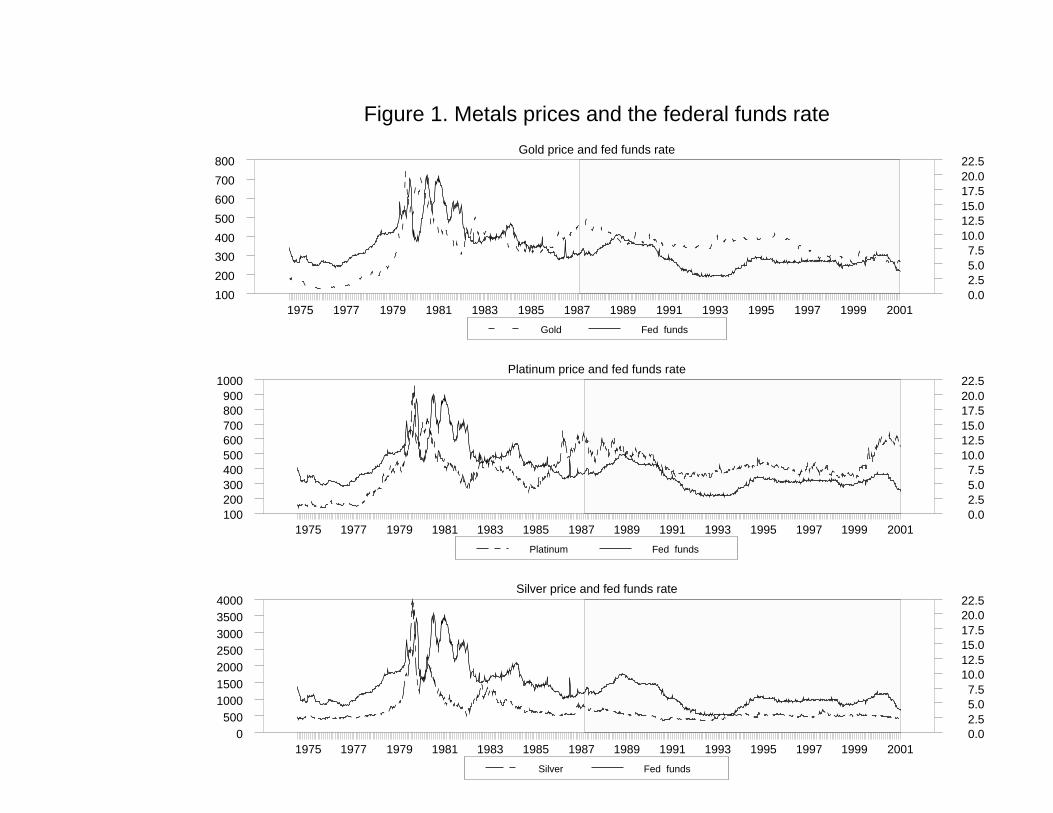
Figure 1 plots the basic weekly data used in the study, again focusing on gold, plat-
inum and silver prices, and the federal funds rate. The shaded area in the graph denotes
Greenspan’s era as board chair. The figure gives an informal view of time series behavior
of these variables, and the statistical relationship between metals prices and the fed funds
rate. First note that the three metals prices are positively correlated over time, and that
this is especially true with respect to gold and platinum, though this correlation appears
to break down after 1999.7 Second, there appears to be a leading relationship between
metals prices and the fed funds rate: broad upward movements in metal prices tend to
be followed at a later date by increases in the funds rate, and vice versa. For example,
the peak in gold prices in mid- to late-1987 and the subsequent decline until early 1993 is
7 Indeed, the correlation breaks down after 1987 – the correlation coefficient betweengold and platinum prices over the full sample is 0.86, but is only 0.15 after August 1987.Over the full sample, the correlation coefficient between gold and silver prices is 0.53 andbetween platinum and silver is 0.44; after Aug. 1987, these coefficients become 0.36 and0.48, respectively.
– 8 –
followed by a peak in the federal funds rate in April 1989 and decline until late 1993.
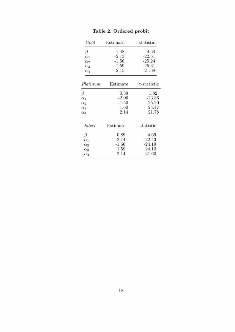
To examine this apparent relationship further, we estimate an ordered probit model,
in which the dependent variable is based on the federal funds rate target, not the actual
rate. While these two variables are closely related, using the target rate eliminates much
of the high frequency noise in the effective rate. The target rate also has the advantage of
being directly linked to policy decisions of the Fed. The ordered response model allows us
to handle the technical difficulties that arise because the target rate is constant over long
periods of time. But most importantly, the model is non-linear and can account for the
possibility that the Fed responds only to large changes in metals prices.
Table 2 reports estimates of the model, for the period 1983 to 2001 (a period over which
the Fed targeted the funds rate; see Meulendyke, 1998, Ch. 2). The dependent variable
is the change in the funds rate target, categorized into large decrease, small decrease, no
change, small increase and large increase, as described above. The independent variable
is the average growth rate of the metals price over a 52 week period. This variable is
lagged by 26 weeks to allow for a delay in the Fed’s response. β measures the effect of the
independent variable on the probability that the funds rate will change to the next highest
category. αi, i = 1, · · ·, 4 denote the thresholds.
In all three cases, a sustained change in the metals price has a positive and statistically
significant (at 10%) effect on the funds rate target – a rising metal price increases the
probability that the target rate will be raised within 26 weeks. The coefficient in the gold
price model is the largest, indicating that the funds rate target is most sensitive to gold
price changes.
The estimated threshold values, which are basically the same across metals, are also
of interest. They indicate non-linearities in the response of the rate target to metals price
– 9 –
growth. The difference between thresholds 2 and 3 is on the order of 3, while the differences
between thresholds 1 and 2, and 3 and 4, are each around 0.5. This supports the idea that
it takes a relatively large change in the metals price to cause the target rate to change at
all, but a smaller change to induce large changes in the target (Vanderhart 2000). Finally,
since the thresholds are symmetric around zero, decreases and increases in the metals price
growth have the same absolute effects on the funds rate target.
We emphasize that one cannot infer causal relationships from these results because we
have not adequately controlled for omitted variables that might jointly affect metals prices
and monetary policy. The ordered probit model is merely a useful way to formalize the
purely statistical relationship over time between metals prices and the funds rate target.
VAR analysis
In this subsection, we report the results of the VAR analysis. We have updated our
earlier study (Lastrapes and Selgin 1995) and extended it to include platinum and silver
prices.
Figure 2 replicates the impulse response functions from the earlier paper, with the
sample period running from August 1987 to April 1994.8 Each panel shows the dynamic
response of a dependent variable to an innovation identified from each of the equations
in the model over a horizon of 150 weeks. For example, the panel in the fourth row and
fourth column plots the response of the price of gold (the fourth variable in the system)
to an innovation, or shock, to the gold market. If such an innovation has no effect on a
variable, the response function would be zero at all horizons. Thus, the response function
is interpreted as the values the variable would take, through time, when an innovation
8 The reserves data differ slightly from the previous study. In that study, total andnon-borrowed reserves were inferred from currency and monetary base data. The slightdifferences that result are unimportant for the focus of this study.
– 10 –
occurs (holding other innovations constant), relative to its values over time if the shock
did not occur.
Given the purpose of this study, the final column is of particular interest. It shows the
dynamic responses of total reserves, non-borrowed reserves, the federal funds rate, and the
price of gold to an innovation in the price of gold (due to unpredictable movements in the
supply and demand for gold). An average shock, over our sample period causes the price
of gold to rise on impact by about 1.4% of its pre-shock value (recall that gold is measured
in logs, so the vertical scale of the panel is in percentage terms). After 12 weeks, the gold
price is about 0.9% higher than it would have been were there no shock, and after a year,
it is only about 0.5% higher. The effect of the shock therefore decays over time with he
price of gold eventually returning to its level before the shock.
Now consider the effect of this shock on the variables representing the instruments of
monetary policy. At the time of the shock, the federal funds rate rises and non-borrowed
reserves fall, indicating a tightening of policy, albeit small (the funds rate rises by about 5
basis points, while non-borrowed reserves fall by around 0.06%). However, the tightening
appears to increase gradually over time – a year after the shock, the funds rate is estimated
to be about 16 basis points higher than its pre-shock value and non-borrowed reserves are
0.2% lower. These response functions are consistent with the notion that the Fed interprets
rising gold prices as an indication of perceived excess liquidity, prompting a monetary
tightening.
The second column shows how the variables in the system respond to monetary policy
shocks; i.e. unanticipated changes due to exogenous Fed policy. Such a shock that raises
non-borrowed reserves in the short-run lowers the fed funds rate, and also causes the gold
price to rise by a maximum of about 1% at a one-month horizon. This finding is consistent
– 11 –
with prior views of the effects of monetary policy on asset prices.
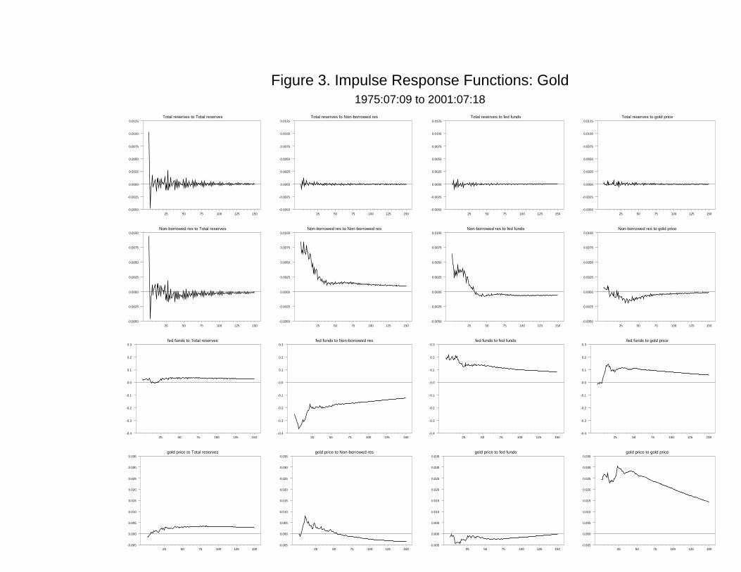
One purpose of this study is to update these findings for other time periods. In Figures
3 through 6, we report the response functions for the VAR with gold estimated over other
samples. Figure 3 reports the results for the VAR when estimated over the full sample
period: 1975 to 2001. The estimates of the responses to gold price shocks are broadly
similar to those for the previous sample, yet there are some differences. The funds rate
and non-borrowed reserves are slower to respond to these shocks, and the funds rate peaks
much sooner (and at a slightly smaller magnitude). At the same time, the gold shock has
a larger effect on gold price, with a maximum effect of around 3% during the first year.
But in any case, there is supporting evidence for a policy response to gold over the full
sample.
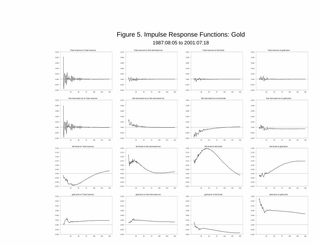
Figures 4 and 5 are for the funds rate targeting period (beginning in 1983) and the
Greenspan era (beginning in August 1987). The results for gold price shocks are again
consistent with those of figure 2, but there is clear weakening of the responses of the policy
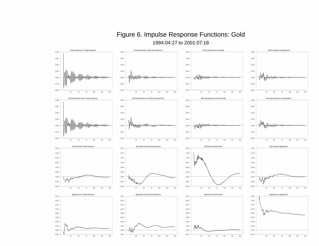
instruments.9 The reason for the weakening is evident from Figure 6: the former tendency
for monetary policy to tighten in the face of gold price shocks breaks down after 1994.
There is virtually no response in non-borrowed reserves in column 4, and while the funds
rate response eventually becomes positive after one year, it is of trivial magnitude.
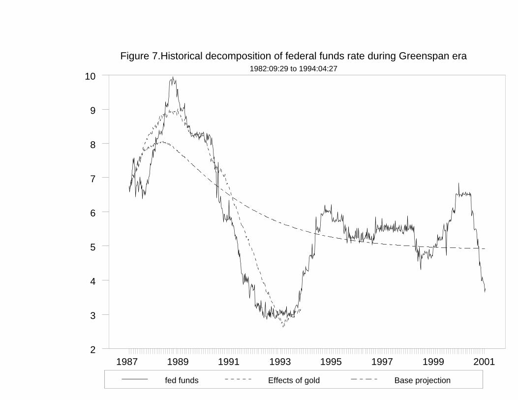
Further statistics that provide some insight into the breakdown of the relationship
between gold and monetary policy after 1994 are plotted in Figures 7 and 8. The plots
decompose the federal funds rate series into a base projection given the estimates from
the VAR and innovations up to the beginning of the Greenspan era, and the contribution
of innovations to the gold price during the Greenspan era. In Figure 7, the estimated
9 Note in Figure 5 that the funds rate responds positively to money supply shocks,which suggests a possible mis-identification of shocks in that case.
– 12 –
model ends uses the sample ending in April 1994, while in Figure 8 the estimated model
ends in July 2001. In Figure 7, we see that the funds rate fluctuates around its projected
value during the Greenspan period: it rises above the projection in 1989 and 1990, and
falls below the projection from late 1990 to the end of the estimated sample (April 1994).
Notice that gold price shocks appear to explain many of these fluctuations, rising and
falling fairly closely with the actual series. On the other hand, Figure 8 suggests that gold
price shocks become much less important in explaining fluctuations around the projection
after 1995.
Gold purchases and sales by central banks over our sample period might have affected
our initial estimates from the VAR. For example, while the Fed might respond to gold prices
in setting policy, it might discount changes in the price that are clearly due to central bank
activity. If central bank activity happened to coincide with unrelated changes in policy, we
might find a spurious relationship between gold prices and the reserve market variables.
To correct for this, we constructed a central bank gold-purchase variable. The variable
is zero over periods of no activity, and takes on the values of purchase and sales during
periods of reported activity. Some judgement was required in constructing this variable,
since some purchases and sales occured over the course of imprecisely defined dates. We
included this variable as an exogenous component of the VAR by adding it to each of
the equations. We also included two dummy variables to account for the Washington
agreement and the Bank of England announcement of reduced sales, both having taken
place in 1999. The results from this extended model (not reported) were essentially the
same as those presented above. This suggests either that Fed activity was orthogonal to
central bank gold activity, or that our measure of central bank gold purchases/sales does
not accurately account for the effect of this activity on the gold market.
– 13 –
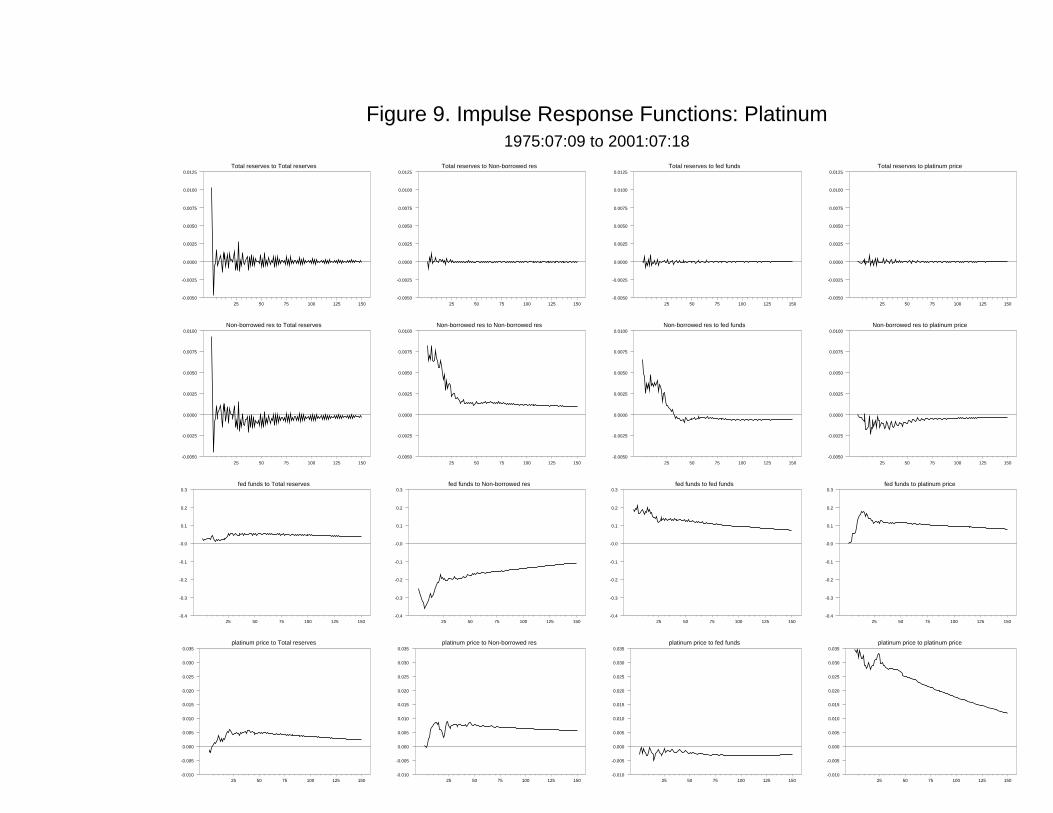
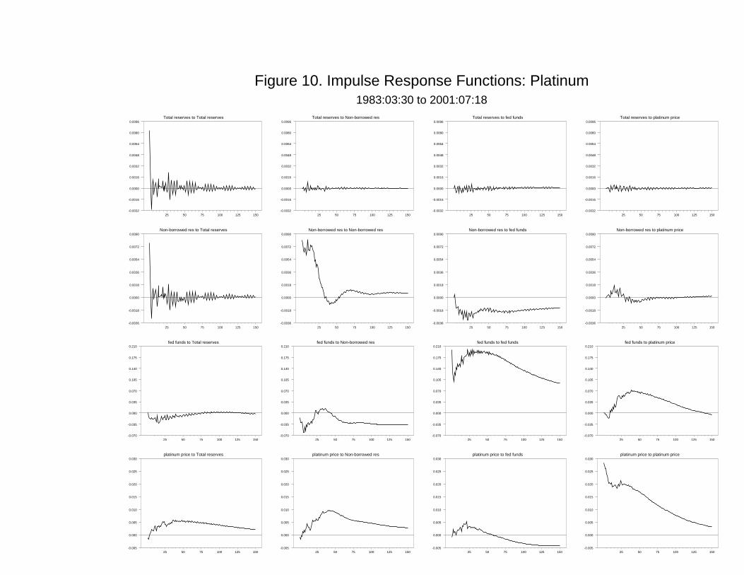
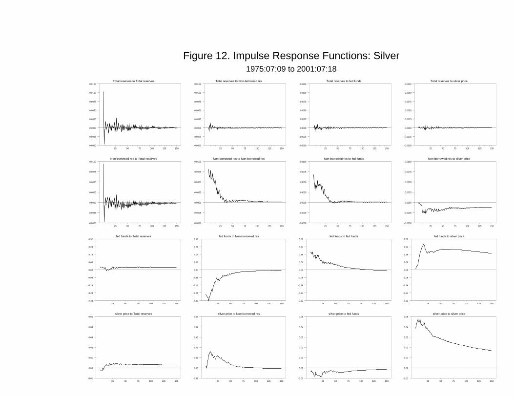
The remaining figures report results from repeating the above exercises for platinum
and silver prices. While the metals are positively correlated over the full sample, the cor-
relation weakens after the late 1980’s. Platinum and silver may therefore contain different
information about excess liquidity than gold prices. Figures 9, 10 and 11 are the results
for platinum over the full sample, the funds rate targeting period (1983 to 2001) and the
period since 1994, respectively; while Figures 12, 13 and 14 are for silver.
The response functions for the first two subsamples are similar to those for gold:
there is evidence of reserve market tightening in the face of positive shocks to the prices
of platinum and silver. Over the full sample, the response of the federal funds rate is
similar across the metals, though its response to silver is larger than for platinum and gold
(the response coefficients peak at around 25 basis points for silver, and less than 20 for
the other metals). Over the funds rate targeting period, the dynamics of the fed funds
response differs across the metals prices. For both platinum and silver, the rate response
is quicker and less persistent that that for gold. In the case of silver, for example, the
funds rate rises by 10 basis points after less than a year after the price shock, while for
gold it takes over twice as long to reach this magnitude. The response of the funds rate
to platinum prices peaks just before one year at 7 basis points, and declines relatively
quickly afterwards. Figures 11 and 14 indicate a similar weakening of policy response to
these metals prices as for the case of gold, although there remains some evidence for policy
reaction to silver prices.
Conclusion
We find evidence consistent with the idea that the Federal Reserve, in setting monetary
policy, has used information contained in gold, platinum and silver prices during the sample
period, 1975 to 2001. However, the relationship appears to have broken down after the mid-
– 14 –
1990’s, for reasons that we cannot determine in this study. Interestingly, the break down
appears to be less drastic for silver than for gold or platinum. Whether or not this implies
that silver currently plays a more predominant role as an indicator to Fed policymakers
than the other metals, or that we have not been able to control for omitted sources of
fluctuations in relative gold and platinum prices, we cannot tell. We can conclude, however,
that Fed behavior toward the price of gold is not a likely explanation for the breakdown
in the correlation between gold and platinum prices that appears to have occurred since
1987.
While we do find some evidence in this study for a Federal Reserve response to metals
prices in setting policy, we do not claim that other information has been irrelevant in
determining monetary policy, or that the relationship we find cannot be attributed to
unobservable variables that affect both policy instruments and metals prices. Further
research should be aimed at examining the current period of policy more closely, and
controlling for other factors that may affect the behavior of the Fed to better infer causal
relationships.10 Even so, awareness of the relationship we document here can assist in the
design of optimal investment portfolios.
10 A potentially insightful approach is to incorporate precious metals prices into estimatesof monetary policy rules as suggested by John Taylor (1993). Such rules estimate therelationship between the Fed’s interest rate instrument and its ultimate policy variables,inflation and the gap between actual output and its potential level. See, for example,Judd and Rudebusch 1998. This strategy would allow us to distinguish the marginalinformation content of precious metals prices, holding constant the information containedin overall prices and output.
– 15 –
References
Enders, Walter, Applied Econometric Time Series, John Wiley & Sons, 1995.
Hamilton, James, Time Series Analysis, Princeton University Press, 1994.
Hamilton, James and Oscar Jorda, “A Model for the Federal Funds Rate Target,”
manuscript, 2000.
Judd, John P. and Glenn D. Rudebusch, “Taylor’s Rule and the Fed: 1970 to 1997,” Federal
Reserve Bank of San Francisco Economic Review, 1998 (3), 3-16.
Lastrapes, William D. and George Selgin, “Gold Price Targeting by the Fed” University
of Georgia, July 1995
Maddala, G.S., Limited-Dependent and Qualitative Variables in Econometrics, Economet-
ric Society Monograph No. 3, Cambridge University Press, 1983.
Meulendyke, Ann-Marie, U.S. Monetary Policy & Financial Markets, Federal Reserve
Bank of New York, 1998.
Strongin, Steven. “The Identification of Monetary Policy Disturbances: Explaining the
Liquidity Puzzle,” Journal of Monetary Economics, 35 (August 1995), 463-97.
Vanderhart, Peter G. “The Federal Reserve’s Reaction Function under Greenspan: An
Ordinal Probit Analysis,” Journal of Macroeconomics, Fall 2000, 631-44.
µ is the sample mean, σ is the sample standard deviation (of the log for the metals prices),µr is the mean weekly return and σr is the sample standard deviation of the weekly (logfor metals prices) difference.