An Ant Colony Optimization Approach to Flexible...

myjournal manuscript No.(will be inserted by the editor)

An Ant Colony Optimization Approach to

Flexible Protein-Ligand Docking

Oliver Korb1, Thomas Stutzle2 and Thomas E. Exner1

1 Theoretische Chemische Dynamik, Universitat Konstanz, Konstanz, Germany

{Oliver.Korb, Thomas.Exner}@uni-konstanz.de2 IRIDIA, CoDE, Universite Libre de Bruxelles, Brussels, Belgium

[email protected]

The date of receipt and acceptance will be inserted by the editor

Abstract The prediction of the complex structure of a small ligand with

a protein, the so-called protein-ligand docking problem, is a central part of

the rational drug design process. For this purpose, we introduce the dock-

ing algorithm PLANTS (Protein-Ligand ANT System), which is based on

ant colony optimization, one of the most successful swarm intelligence tech-

niques. We study the effectiveness of PLANTS for several parameter settings

and present a direct comparison of PLANTS’s performance to a state-of-

the-art program called GOLD, which is based on a genetic algorithm and

frequently used in the pharmaceutical industry for this task. Last but not

least, we also show that PLANTS can make effective use of protein flexibility

giving example results on cross-docking and virtual screening experiments

for protein kinase A.

1 Introduction to the Protein–Ligand Docking Problem

The pharmacological effect of a drug relies in many cases on the formation

of a complex between a small chemical compound, the drug called ligand

in the following, and a macromolecule, the protein, whose malfunction is

provoking a disease. For the rational design of new drugs against a target

protein, the specific interactions between both complex partners must be

correctly predicted and optimized. This task is notoriously time-consuming

2 Oliver Korb, Thomas Stutzle and Thomas E. Exner

and expensive taking up to 15 years [1] and costing several hundred million

euros.

This drug design process pursued by major pharmaceutical companies

begins with the identification of a suitable protein target, where a potential

drug could interfere to fight a disease. For this target, specific assays are

developed, which are then used in high-throughput screening experiments to

test the biological activity of large databases of possible drug candidates.

Molecules with high affinity, so-called lead structures, are then chemically

varied (lead optimization cycle) and the most potent ones of the resulting

candidates are transferred to the preclinical and finally the clinical test

phase.

Today, most of these steps are guided by computer experiments. Very

large databases, ranging in size from thousands to millions of ligands, can

be tested by ligand- or structure-based virtual screening techniques and

different lead-optimization routes can be tried without ever synthesizing

most of the compounds. Structure-based approaches, like the one presented

in this publication, start with a known 3D structure of a protein. These

structures are obtained by experimental techniques like X-ray crystallog-

raphy or NMR-spectroscopy and are, for example, publicly available from

the protein data bank (PDB) [2]. Then, a docking algorithm tries to solve

the pose prediction problem. This problem consists in finding the correct

orientation and conformation (that is, the atoms’ spatial arrangement re-

sulting from rotations about rotatable single-bonds) of the ligand within the

a priori known active site of the protein. In the context of virtual screening,

additionally different ligands must be ranked correctly according to their

binding affinity.

The underlying so-called protein-ligand docking problem (PLDP) was

first formulated by Fischer using the famous lock-and-key metaphor [3]:

The key (ligand) must fit exactly into the lock (protein) to open the door

(pharmacological effect). But because molecules are not rigid objects, this

description is too limited and at least the flexibility of the ligand must be

taken into account, which is done by almost all state-of-the-art docking

algorithms. But even the protein conformation can adapt to an incoming

ligand, leading to the so-called induced fit model [4]. In particular, if the

protein structure that has been determined without any bound ligand, the

so-called apo form, is used, large rearrangements at the active site of the

protein may be observed. Therefore, whenever possible, a 3D-structure of

a protein complexed with a known ligand, a holo form, is used under the

Title Suppressed Due to Excessive Length 3

assumption that a potential new drug would bind to an extremely similar

protein conformation. The validity of this assumption is apparent in many

cases when comparing different holo forms of a same protein cocrystallized

with different ligands whose structures are stored in the PDB.

2 Computational Approaches to the Docking Problem

A large variety of approaches for solving the PLDP have been proposed.

Broadly, these can be classified as fragment-based methods, which split

the ligand into different parts and perform an incremental construction, as

stochastic optimization methods, or as multiconformer docking approaches

(see [5] and references therein). In this paper, we focus on the second class.

Stochastic optimization methods are based on the formulation of the PLDP

as an optimization problem and on the use of stochastic search methods

for searching optimal solutions. The optimization problem is defined by an

objective function f and the search space. In the context of the PLDP,

the objective function is usually called scoring function and it estimates

the binding energy between the protein and the ligand; the search space is

given by the degrees of freedom of the protein and the ligand. Given these

two components, the PLDP can be seen as the problem of searching for the

values of the degrees of freedom that globally minimize the scoring function.

In most approaches, the protein structure is kept rigid. In this case, the

task is to find the best possible orientation of the ligand with respect to the

protein by changing the ligand’s translation and rotation as well as changing

the torsion angles of single bonds in the ligand that are not part of a ring

system. In the optimization version of the PLDP, these degrees of freedom

correspond to continuous variables that define the transformation applied.

Hence, the task is to find optimal values for the ligand’s 3 translational,

3 rotational and rl torsional degrees of freedom, describing the rotations of

single bonds. Thus, the total number of variables, that is, the dimension of

the optimization problem, equals n = 6 + rl. In more advanced methods,

like the approach presented here, small changes in the conformation of the

protein can be modeled by introducing flexibility to specific amino-acid side-

chains in the active site. This adds one torsional degree of freedom for each

rotatable bond in the flexible side-chains. Therefore, the problem dimension

becomes n = 6 + rl + rp for a ligand with rl and a protein with rp torsional

degrees of freedom.


A wide repertoire of optimization strategies have been proposed for find-

ing the global minimum energy structure, which is expected to correspond to

the experimentally determined complex structure. These include genetic al-

gorithms that are used in the programs GOLD [6] and AutoDock [7], Monte

Carlo minimization in the programs ICM [8] and QXP [9], and simulated

annealing, evolutionary programming, and tabu search in PRO LEADS [10].

Recent studies [11,12] compared different docking tools on a large test

set of experimentally determined complex structures. They reported success

rates of 30 to 60%, where the success rate is defined as the percentage of

complexes for which the predicted structure with the lowest energy is very

close (root mean square deviation within 2.0 A) to the experimentally de-

termined structure. Therefore, it can be concluded that a universal docking

tool that has excellent predictive capabilities across many complexes is not

available at the moment. When we consider, as we do in this paper, stochas-

tic optimization methods, this lack of performance can be attributed to the

scoring problem and the sampling problem. Currently, there exists no scor-

ing function capable of performing correct measurements for all given input

structures. But even if there was a perfect scoring function, there would still

be the problem that there is no guarantee that the correct binding mode of

the ligand, that is, the ligand conformation as observed in the crystal struc-

ture, is actually found by the sampling algorithm. On the one hand, this

can be caused by the fact that the native complex structure is not accessible

with the limited flexibility of the protein accounted for in the algorithms.

On the other hand, introducing additional degrees of freedom may result in

additional scoring function failures or make the problem more difficult due

to the increased dimension of the search space.

3 PLANTS

We have developed Protein–Ligand ANT System (PLANTS), the first ACO

algorithm for tackling the PLDP. PLANTS is a stochastic search algorithm

that treats the ligand and the protein as flexible, which means that there

are 6 + rl degrees of freedom for the ligand and rp torsional degrees of

freedom for the protein as described above. Even if no flexible side-chains

are specified, PLANTS partially considers the flexibility of the protein by

allowing for the optimization of the positions of hydrogen atoms that could

be involved in hydrogen bonding; this results in rp = rdon torsional degrees

of freedom, where rdon is the number of rotatable hydrogen bond donor


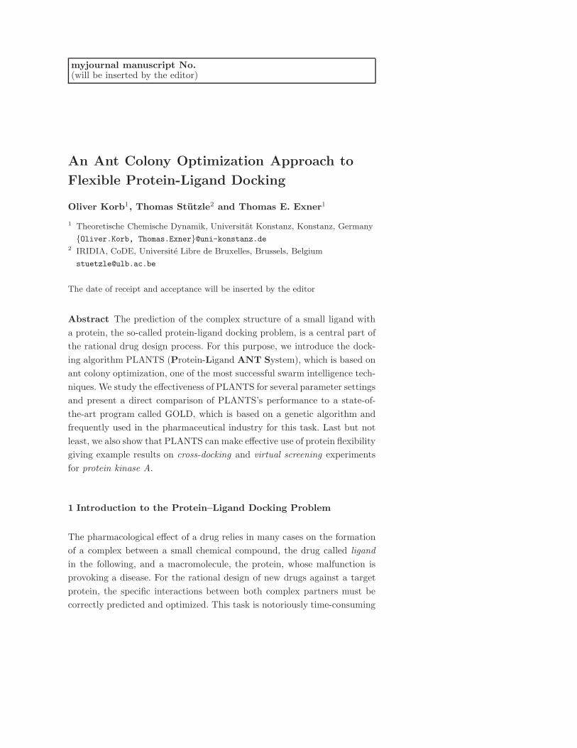
Figure 1 This figure illustrates the degrees of freedom for the docking problem.

It shows the origin of the ligand’s coordinate system as a sphere. The large arrows

indicate the ligand’s translational degrees of freedom; they also are the axes of ro-

tation. The small arrows mark the ligand’s rotatable bonds and also the rotatable

bonds of a single protein side-chain (upper right corner), which emanates from

the protein surface that is shown in the background.

groups (OH- and NH+3 -groups) available in the protein binding site. Both

the ligand’s and the protein’s degrees of freedom are illustrated in Figure 1.

The resulting minimization problem to be solved by PLANTS can be

formulated as

minx∈Rn

f(x) : Rn → R. (1)

In this equation, f is the objective function, also called the scoring func-

tion, x = [x1, . . . , xn]t ∈ Rn represents the ligand’s and the protein’s degrees

of freedom and n = 6+rl+rp is the problem dimension. Hence, the problem

is a continuous optimization problem, where the angles can be in the domain

[0◦, 360◦) and the intervals of the domains for the translational degrees are

defined by the size of the protein’s binding site.

Pheromone model. The space searched by PLANTS is defined by the lig-

and’s translational, rotational and torsional degrees of freedom as well as

the protein’s torsional degrees of freedom. Since ACO is initially designed

for solving combinatorial problems, we decided to discretize the continuous

variables and to apply existing ACO algorithms, in particular MAX–MIN


Ant System (MMAS) [13], to the problem. The discretization uses for each

of the three translational degrees of freedom an interval length of 0.1A, while

for the three rotational degrees of freedom and all torsional degrees of free-

dom an interval length of 1◦ was taken, resulting in 360 values for the latter.

The number of values for each translational degree of freedom depends on

the diameter of the pre-defined size of the binding site. For the complexes

studied here, this discretization results in 120 to 400 discrete points for each

dimension x, y and z. Each degree of freedom i has associated a pheromone

vector τi with as many entries as values resulting from the discretization.

A pheromone trail τij then refers to the desirability of assigning the value

j to degree of freedom i.

ACO algorithm. The (artificial) ants in PLANTS construct solutions by

selecting one value for each degree of freedom taking into account the phe-

romone values. In an earlier paper [14], we have shown that heuristic infor-

mation was not essential for high performance and, hence, we removed it

in this more recent version of PLANTS. In the solution construction, the

order of the degrees of freedom is arbitrary, since each degree of freedom

is treated independently of the others. For each degree of freedom i, the

probability pij of assigning the value j to an ant is computed as

pij =τij

∑ni

l=1 τil

. (2)

In this equation, ni is the number of values for degree of freedom i. As usual

in MMAS, after each iteration only one solution deposits pheromone; in

PLANTS, this is the best solution generated in the current iteration, sib.

The pheromone update is defined as

τij(t + 1) = (1 − ρ)τij(t) + Iibij (t)∆τ ib (t), (3)

where

∆τ ib(t) =

{

|f(sib)| if f(sib) < 0

0 otherwise,(4)

f(sib) is the value of the scoring function for sib, and ρ is a parame-

ter steering the pheromone evaporation. For a translational degree of free-

dom i, Iibij (t) is one, if sib assigned to i a value in {j − 1, j, j + 1}; for

rotational and torsional degrees of freedom, Iibij (t) is one if a value in

{j − 2, j − 1, j, j + 1, j + 2} mod ni was taken; otherwise it is zero. In

this way, for each degree of freedom not only one single value receives some

pheromone but also the neighboring values. This can be useful to increase


the search diversification. The choice of Equation 4 is based on the fol-

lowing reasoning: strongly negative values of our scoring function indicate

high affinity, that is, the larger the absolute value the better; positive val-

ues would actually correspond to negative affinity and, hence, they do not

receive any positive feedback. In the latter case, no pheromone is deposited

in an iteration. In PLANTS, MMAS’s lower and upper pheromone trail

limits, τmin and τmax, are set as follows: τmax = |f(sdb)|/ρ, where f(sdb)

is the best scoring function value found since the last search diversification

(the search diversification used is explained below); the values for τmin are

calculated for each degree of freedom i as

τmini=

τmax · (1 − n√

pbest)

(ni − 1) · n√

pbest, (5)

following the formulas given in [13]. In this equation, n is the problem

dimension, that is, the number of degrees of freedom, ni is the number of

values that resulted from the discretization of degree of freedom i, and pbest

is the probability of the best solution to be reconstructed assuming that the

colony has already converged [13].

Local search. As in most applications of ACO algorithms to NP-hard prob-

lems, we also improve candidate solutions by a local search algorithm [15].

However, differently from most of such combinations that have been pro-

posed earlier, in PLANTS the ants and the local search algorithm search

in two different search spaces: while the ants work on the discretized search

space, the local search works in the continuous search space defined by the

translational, rotational and torsional degrees of freedom of the ligand and

the protein. In fact, the resulting, very high performing algorithm for the

PLDP indicates that such a combination may also be interesting for other

nonlinear continuous optimization problems.

We use the simplex local search algorithm described by Nelder and Mead

(NMS) for nonlinear, continuous function optimization [16]. A simplex is a

polytope of n + 1 vertices in an n-dimensional space. The NMS algorithm

transforms the points of a given starting simplex by using the operations

reflection, expansion and contraction until the fractional range from the

highest to the lowest point in the simplex with respect to the function

value is less than a tolerance value, which we choose as 0.01, or a maximum

number of function evaluations is reached (we set this limit to 5000 function

evaluations); for details on the algorithm we refer to [17]. As the parameter


settings in the NMS algorithm we use ∆trans = 2A, ∆rot = 90◦ and ∆tors =

90◦ for the construction of the initial simplex.

In PLANTS, all ants improve their solution by applying NMS. The start-

ing simplex is defined by the initial, unmodified solution of each ant and the

other n by adding the specific offsets to each variable. Note that the NMS

algorithm does not necessarily stop in a local optimum and, hence, the final

solution could be further improved by re-applying NMS. In fact, we do so

and use NMS again to further improve the solution of the iteration-best

ant. This refinement local search, which uses the same parameter settings

as given above, is restarted until the improvement in the scoring function

obtained by one application of NMS is less than 0.2.

Algorithmic outline. An algorithmic outline of PLANTS is given in Algo-

rithm 1. Essentially, PLANTS follows the typical scheme of solution con-

struction, local search, and pheromone update that is followed in virtually

all ACO algorithms for NP-hard combinatorial optimization problems [15].

Some additional details are explained next.

The procedure InitializeParametersAndPheromones sets the initial param-

eter values, sets up the ligand and the protein for processing, and initializes

the pheromone trails to a very large value such that after the first iteration

all pheromone trails correspond to τmax.

The number of iterations for PLANTS is determined by the formula

max iterations = σ · 10

m· (100 + 50 · lrb + 5 · lha), (6)

where σ is a parameter used for scaling the number of iterations, m is the ant

colony size, lrb is the number of rotatable bonds and lha the number of non-

hydrogen atoms in the ligand. Hence, the maximum number of iterations

depends on the ligand: very flexible and large ligands get more search time

than rigid and small ones.

The procedures ConstructSolution and LocalSearch implement the solu-

tion construction and the NMS local search algorithm, respectively. Once

for each ant a solution is generated, the iteration-best solution sib is de-

termined by the procedure GetBestSolution. The procedure RefinementLo-

calSearch then applies the additional local searches to sib, as described in

the previous subsection. Next, the procedure UpdatePheromones manages

the pheromone update and checks the pheromone trail limits.

PLANTS also applies additional search diversification in procedure Ap-

plySearchDiversification. Search diversification consists, in the first place, of


algorithm 1 PLANTS

InitializeParametersAndPheromones()

for i = 1 to max iterations do

for j = 1 to ants do

sj ← ConstructSolution()

s∗j ← LocalSearch(sj)

M ←M ∪ s∗j

end for

sib ← GetBestSolution()

sib ← RefinementLocalSearch(sib, 0.2)

M ←M ∪ sib

UpdatePheromones(sib)

if diversificationCriteriaMet then

ApplySearchDiversification()

end if

end for

return M

pheromone trail smoothing as proposed in [13], using a smoothing factor of

0.5. If three smoothings have been done, all pheromone trails are erased and

set to their initial value. In fact, this latter diversification corresponds to

a complete restart of the algorithm. Search diversification is invoked each

time more than 10 consecutive iteration-best solutions differ by less than

0.02 · |f(sdb)|, where sdb is the best solution found since the last search

diversification.

Once PLANTS terminates, the set of all solutions (M) returned by the

procedures LocalSearch and RefinementLocalSearch is output; this set M also

contains the overall best solution found by PLANTS. The solutions in set

M then undergo a post-processing phase.

Post-processing. Once PLANTS finishes its search, all solutions that were

generated are post-processed to output a number of diverse, high-quality

conformations. This is done by first sorting all the solutions in M according

to increasing scoring function values. Then, PLANTS extracts a specified

number of ligand structures, typically 10, such that the minimal root mean

square deviation (RMSD) between any of the extracted structures is larger

than 2 A. These solutions can then be used for rescoring with other, more

advanced scoring functions, which may be computationally too demanding

to be directly used in the optimization process. Experimentally, it has been

found that rescoring can increase the chance of finding a ligand conformation


F

E

A B DC

r

PLP(

r)

A

D

βr

α

(a) (b)

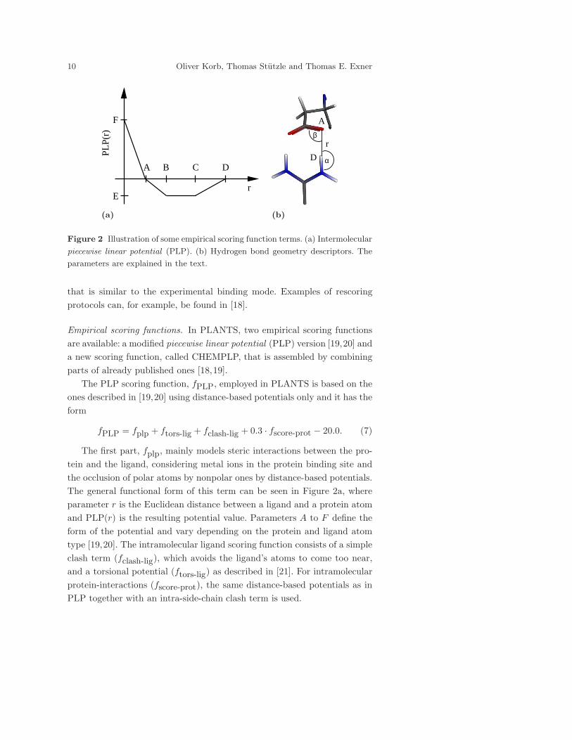
Figure 2 Illustration of some empirical scoring function terms. (a) Intermolecular

piecewise linear potential (PLP). (b) Hydrogen bond geometry descriptors. The

parameters are explained in the text.

that is similar to the experimental binding mode. Examples of rescoring

protocols can, for example, be found in [18].

Empirical scoring functions. In PLANTS, two empirical scoring functions

are available: a modified piecewise linear potential (PLP) version [19,20] and

a new scoring function, called CHEMPLP, that is assembled by combining

parts of already published ones [18,19].

The PLP scoring function, fPLP, employed in PLANTS is based on the

ones described in [19,20] using distance-based potentials only and it has the

form

fPLP = fplp + ftors-lig + fclash-lig + 0.3 · fscore-prot − 20.0. (7)

The first part, fplp, mainly models steric interactions between the pro-

tein and the ligand, considering metal ions in the protein binding site and

the occlusion of polar atoms by nonpolar ones by distance-based potentials.

The general functional form of this term can be seen in Figure 2a, where

parameter r is the Euclidean distance between a ligand and a protein atom

and PLP(r) is the resulting potential value. Parameters A to F define the

form of the potential and vary depending on the protein and ligand atom

type [19,20]. The intramolecular ligand scoring function consists of a simple

clash term (fclash-lig), which avoids the ligand’s atoms to come too near,

and a torsional potential (ftors-lig) as described in [21]. For intramolecular

protein-interactions (fscore-prot), the same distance-based potentials as in

PLP together with an intra-side-chain clash term is used.


Scoring function CHEMPLP, denoted as fCHEMPLP has the following

functional form:

fCHEMPLP = fplp +fchem-hb+ftors-lig +fclash-lig +0.3 ·fscore-prot−20.0

(8)

The first part (fplp) of the intermolecular score uses the above described

version of the PLP scoring function, although with different parameter set-

tings. The second part, (fchem-hb) considers the hydrogen bonding and

metal-acceptor interactions between the protein and the ligand as done in

GOLD’s CHEMSCORE implementation [18]. Figure 2b shows an illustra-

tion of the parameters used to define the hydrogen bond geometry. The

Euclidean distance r between the hydrogen bond donor atom D (donor)

and a hydrogen bond acceptor atom A (acceptor) as well as the donor angle

α and the acceptor angle β influence the strength of the hydrogen bond

depending on their deviation from a given set of ideal values. This part

has been modified to differentiate between charged and neutral hydrogen

bonds and to allow for the scoring of weak CH–O interactions [22]. The

intramolecular ligand and protein terms are the same as described in the

PLP case.

Finally, a penalty term is added to both scoring functions if the ligand’s

reference point falls outside the predefined binding site of the protein. The

development of these empirical scoring functions was, together with the

design of the search algorithm, a major contribution of our work; the devel-

opment of the scoring function will be covered in a forthcoming publication.

4 Parameter Optimization

In an earlier paper on PLANTS [14], the influence of the number of ants, the

pheromone evaporation ρ, the heuristic information and the factor σ, which

scales the number of iterations, was investigated. It turned out that using

20 ants in conjunction with a setting of ρ = 0.25 seems to result in overall

good performance across different settings of σ. The heuristic information

was found to have not a significant impact on performance and, hence, we

removed it from further consideration in our current version of PLANTS.

These earlier tests were all carried out using a setting of 0.9 for parameter

pbest, which directly affects the lower pheromone trail limit τmin and, hence,

also the explorative power of the algorithm. In this paper, we study the

parameters that influence the diversification behavior of the algorithm. In


this context, the parameters pbest and the evaporation rate ρ are of special

interest.

Two subsets comprising 15 complexes (for scoring function CHEMPLP)

and 11 complexes (for scoring function PLP) from the CCDC/Astex dataset

[23] with ligands having between two and ten rotatable bonds have been used

for the parameter variation. These subsets were removed from the final test

set used for the large-scale tests described in the next section. We varied

the parameters σ, ρ and pbest considering three to seven values for each

(the values tested are indicated in Figure 3), which resulted in 84 distinct

parameter configurations. On each complex, PLANTS was run for 25 inde-

pendent trials. We measured for each configuration the average success rate,

the average computation time and the average number of function evalua-

tions. The success rate is defined as the percentage of complexes for which

the top-ranked docking solution is within an RMSD of 2.0 A of the exper-

imentally determined binding mode as given in the CCDC/Astex dataset

[23]. The computation times in this section are given in seconds on a single

core of a Dual Core AMD Opteron 870, 2.0GHz CPU; protein setup time

(6 s on average) and ligand setup time (0.01 s on average) are excluded.

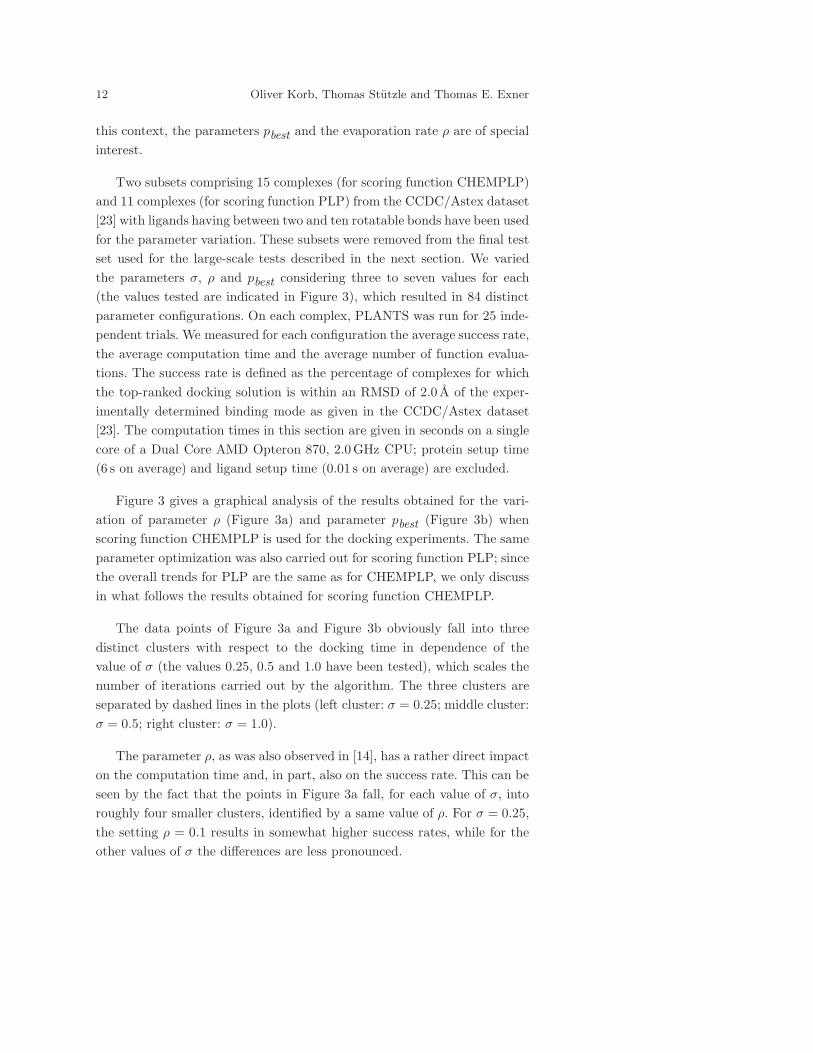
Figure 3 gives a graphical analysis of the results obtained for the vari-

ation of parameter ρ (Figure 3a) and parameter pbest (Figure 3b) when

scoring function CHEMPLP is used for the docking experiments. The same

parameter optimization was also carried out for scoring function PLP; since

the overall trends for PLP are the same as for CHEMPLP, we only discuss

in what follows the results obtained for scoring function CHEMPLP.

The data points of Figure 3a and Figure 3b obviously fall into three

distinct clusters with respect to the docking time in dependence of the

value of σ (the values 0.25, 0.5 and 1.0 have been tested), which scales the

number of iterations carried out by the algorithm. The three clusters are

separated by dashed lines in the plots (left cluster: σ = 0.25; middle cluster:

σ = 0.5; right cluster: σ = 1.0).

The parameter ρ, as was also observed in [14], has a rather direct impact

on the computation time and, in part, also on the success rate. This can be

seen by the fact that the points in Figure 3a fall, for each value of σ, into

roughly four smaller clusters, identified by a same value of ρ. For σ = 0.25,

the setting ρ = 0.1 results in somewhat higher success rates, while for the

other values of σ the differences are less pronounced.


(a)

70

75

80

85

90

95

100

0 10 20 30 40 50

success r

ate

[%

]

time [s]

rho 0.1 rho 0.15

rho 0.2 rho 0.25

(b)

70

75

80

85

90

95

100

0 10 20 30 40 50

success r

ate

[%

]

time [s]

pbest 0.01 pbest 0.1 pbest 0.5

pbest 0.9 pbest 0.99

Figure 3 Influence of different settings for (a) evaporation factor ρ and (b) pa-

rameter pbest with respect to the average success rate and docking time for scoring

function CHEMPLP. For the sake of clarity, the data points for pbest = 0.3 and

pbest = 0.7 are not shown as they were anyway not part of the optimal parameter

set. For further explanations see the text. Note that the zooms of the individ-

ual clusters differ in their x/y-ratio slightly from the original plot to improve the

visibility of the distribution of the points.


Concerning the parameter pbest, no clear trend is apparent and the con-

clusion is that the performance of PLANTS is not very sensitive with respect

to pbest.

For the sake of having a same set of parameter values across different

values of σ, we use a setting of ρ = 0.15 and pbest = 0.5 in the case of

scoring function CHEMPLP as well as ρ = 0.15 and pbest = 0.1 for scoring

function PLP when performing tests on a large set of benchmark instances.

Hence, all the experiments presented in the next section differ only in the

setting of parameter σ, which allows to directly trade between computation

time and success rates.

5 Pose Prediction

The clean list of the comprehensive CCDC/Astex dataset [23] has been

used for the validation of PLANTS. From these 224 complexes, 11 include

covalently bound ligands and were removed, because PLANTS does not

provide a covalent docking functionality at the moment. Additionally, also

the 15 complexes used during the parameter optimization process described

in section 4 were removed to avoid a bias in favor of PLANTS. Hence, our

test set consists of 198 non-covalently bound complexes that we call clean

listnc. The number of rotatable bonds of the ligands in clean listnc ranges

from 0 to 28. For all experiments, the spherical binding site as defined in

the CCDC/Astex dataset was used to determine the search space for the

ligand’s translational degrees of freedom. Before each docking run, the lig-

and structures were randomized with respect to the translational, rotational

and torsional degrees of freedom, that is, the ligands’ conformations as ob-

served in the crystal structures were changed to random conformations to

avoid biasing the results. The best parameter settings determined in the

last section were then tested on the whole clean listnc. The applied param-

eter setting as well as the success rate for the (i) top-ranked solution, (ii)

solutions up to rank 3 and (iii) solutions up to rank 10 (ranks with respect

to the solutions in the order as returned by the post-processing—a success

is obtained if among these highest ranked ligands one has an RMSD lower

than 2 A compared to the experimentally determined complex structure)

and the average docking time along with the number of scoring function

evaluations are presented in Table 1 (see upper and middle part marked

with PLANTS). All calculations were carried out on a Pentium 4 Xeon,

2.8GHz CPU.


Table 1 Results on 198 complexes of clean listnc for PLANTS (scoring func-

tion CHEMPLP and PLP) and GOLD (scoring function GOLDSCORE) for se-

lected parameter settings averaged over 25 independent experiments. For all tests

a colony size of 20 ants was used. Standard deviations for the success rates are

given in parentheses.

PLANTSCHEMPLP

success rate (%) up to rank

σ 1 3 10 time (s) eval. (106)

0.25 62.93 (2.58) 74.71 (1.95) 80.75 (2.01) 27.85 1.02

0.40 65.78 (2.09) 78.14 (1.48) 84.30 (1.34) 43.98 1.61

1.00 71.94 (1.84) 83.94 (1.48) 89.62 (1.46) 110.07 3.99

2.00 73.80 (1.37) 86.40 (1.35) 92.04 (1.43) 217.04 7.92

PLANTSPLP


σ 1 3 10 time (s) eval. (106)

0.50 62.44 (2.00) 75.52 (1.64) 83.19 (1.65) 22.25 1.26

1.00 64.32 (1.51) 78.55 (1.13) 86.16 (1.46) 45.24 2.50

2.00 65.25 (0.93) 79.76 (1.33) 87.72 (1.44) 89.64 4.98

5.00 66.08 (1.08) 80.57 (1.16) 89.43 (1.35) 218.97 12.41

GOLDGOLDSCORE


autoscale 1 3 10 time (s) eval. (106)

0.10 65.94 (1.56) 72.61 (1.26) 77.19 (1.51) 43.47 n.a.

0.30 67.94 (1.90) 74.16 (1.88) 80.08 (2.12) 118.84 n.a.

1.00 72.12 (1.57) 76.81 (1.53) 81.31 (1.23) 318.02 n.a.

For PLANTSCHEMPLP, the success rates for the top-ranked solutions

range from about 62.9% at average docking times of approximately 28 s

(σ = 0.25) to 73.8% at average docking times of 217 s (σ = 2) for each

complex. Considering solutions up to rank 3 and 10 even higher success

rates of up to 92% can be achieved. This is especially interesting for vir-

tual screening applications where rescoring of these structures with another

scoring function could in principle identify the correct pose. In dependence

of the available computational resources, the time frame and the size of the

ligand database to be screened (which can be in the order of thousands to

millions of compounds), a potential user may choose one of the parameter


0

20

40

60

80

100

27-2924-2621-2318-2015-1712-149-116-83-50-2

avg

. su

cce

ss r

ate

[%

]

# ligand rotatable bonds

PLANTS1.0 GOLD0.3 # complexes

Figure 4 Average success rates in dependence of the number of ligand rotatable

bonds for PLANTSCHEMPLP (σ = 1) and GOLDGOLDSCORE (autoscale = 0.3 ).

Additionally, the number of complexes for each interval of ligand rotatable bonds

is shown by the dotted line.

configurations presented here. As a guideline we suggest to use a setting

of 20 ants, σ = 1, ρ = 0.15 and pbest = 0.5 as the standard setting for

PLANTS.

Using the other scoring function available in PLANTS, PLP, the al-

gorithm reaches success rates ranging from about 62% at average search

times of around 22 s to about 66% at average docking times of 219 s per

complex considering the first-ranked solutions only. For low computation

time limits, the results of PLANTSPLP are reasonably close to those ob-

tained by using PLANTSCHEMPLP. This suggests that PLANTS profits from

the additional hydrogen bonding terms available in CHEMPLP especially

for higher computation times. In fact, PLANTSPLP seems to reach limiting

behavior at success rates of about 66%, given that an increase of σ from

two to five has only a negligible effect on increasing the success rate. This

trend can be confirmed by statistical tests on the significance of the differ-

ences in the success rates. Using the binomial test with significance level

α = 0.05 for PLANTSCHEMPLP and PLANTSPLP for σ = 0.4 and σ = 1.0

respectively (this results in similar average computation times), no signifi-


cant difference between the two could be detected; however, for a setting of

σ = 2.0 and σ = 5.0 for PLANTSCHEMPLP and PLANTSPLP respectively, the

null hypothesis had to be rejected at the α = 0.05 level. A similar trend is

true when looking at the results up to rank three and ten. In this case, for

short computation times PLANTSPLP sometimes even gives slightly higher

success rates for comparable computation times, while for the longer com-

putation times PLANTSCHEMPLP becomes preferable. (When comparing the

same settings of σ for PLANTSCHEMPLP and PLANTSPLP, only the differ-

ence between the success rates up to rank three for the longer computation

times are statistically significantly different.)

For comparison, the lower part of Table 1 shows the results on the same

test set for GOLD (Genetic Optimisation for Ligand Docking) [6,18], a

state-of-the-art docking program that is frequently used in the pharmaceu-

tical industry. The genetic algorithm optimizes mappings of possibly corre-

sponding hydrogen bonding atoms and hydrophobic groups in the protein

and the ligand as well as the ligand’s torsional degrees of freedoms and the

orientation of hydrogen bond donor groups in the protein. In each GA-step,

a matching procedure tries to minimize the distance between the mapped

fitting points. Additionally, problem-specific knowledge like torsion-angle

libraries for the ligands’ rotatable bonds as well as a cavity detection al-

gorithm for restricting the search space for possible ligand placements is

employed.

Ideally, when comparing the two approaches, both programs should use

the same scoring function to focus the comparison on the impact of the

search algorithms (or, if the scoring functions are of interest, these are tack-

led using the same search algorithm). However, integrating either of the

scoring functions into the other program package is first of all a non-trivial,

time-consuming task and second it inherently has the problem that the

reimplementation and the original may not correlate perfectly. Additionally,

changing the scoring function requires the search algorithm to be adapted

and fine-tuned as well, making it possibly very different from the original

implementation. Hence, we rather opted for comparing the two programs’

performance as a whole. There are good reasons for doing so. Firstly, this

allows to compare the performance of PLANTS to a recognized state-of-the-

art package for the same task; secondly, this comparison is also relevant for

practice, where the algorithms would be used out-of-the-box for a particular

docking task.


For the experiments presented in this section, GOLD version 3.0.1 has

been employed. We tested three settings for parameter autoscale, which

automatically chooses appropriate GA search settings in dependence of the

given protein binding site and the ligand molecule. The maximum number

of GA runs per ligand was set to 10, early termination and cavity detection

were activated and Goldscore (GOLDGOLDSCORE) was used as the scoring

function.

When comparing the success rates obtained by PLANTSCHEMPLP to those

of GOLDGOLDSCORE at similar or slightly lower average computation times

given in Table 1 (that is, settings of σ ∈ {0.4, 1.0, 2.0} for PLANTSCHEMPLP),

PLANTSCHEMPLP reaches always higher success rates with the only excep-

tion being the very minor difference in favor of GOLDGOLDSCORE for the

top-ranked solution at a setting of σ = 0.4 for PLANTSCHEMPLP. (The bi-

nomial test at α = 0.05 for equality of success rates was rejected in favor

of PLANTSCHEMPLP for all pair-wise comparisons of the success rates up to

rank three and ten.) Hence, this clearly shows that PLANTS’s performance

is at least comparable to that of GOLD, which is a very encouraging result.

Finally, more detailed information on the success rate of PLANTSCHEMPLP

versus GOLDGOLDSCORE in dependence of the number of rotatable ligand

bonds is given in Figure 4, which again confirms the competitiveness of

PLANTS.

6 Protein Flexibility

The pose prediction tests carried out in the previous section for the clean

listnc were ideal test cases in the sense that the ligands were docked back

into their native protein structures. When performing a virtual screening ex-

periment, however, usually only a single protein structure is available where

all biologically active ligands should fit into with the correct conformation.

As already mentioned in the introduction, upon ligand binding the protein

may undergo small or sometimes even large rearrangements, in which case

a single rigid protein structure may not be able to reproduce the poses of all

ligands correctly. In this section, we deal with exactly this type of problem

and examine the influence of protein flexibility during docking and virtual

screening. In fact, the importance of protein flexibility is now widely rec-

ognized and very recent versions of some docking algorithms like GOLD

include the treatment of induced fit effects.


Figure 5 Superimposition of the eight PKA protein structures (the protein

backbones are illustrated as tubes). In the lower left corner the side-chain confor-

mations of residue PHE327 for each protein structure are shown (for the sake of

clarity all other residues are hidden). Ligand staurosporine (shown in the middle

along with all other ligands) clashes with this residue in all non-native structures

(marked with a bold circle).

6.1 Cross-Docking

As a first step, we test PLANTS with respect to its ability to reproduce bind-

ing modes of different ligands also in non-native protein structures of the

same target, a type of experiment called cross-docking. The cross-docking

experiment was carried out for protein kinase A (PKA), which is a promis-

ing target in breast-cancer research. For this experiment, we have used eight

PKA protein structures (seven holo forms and one apo form). We used PDB-

entries 1Q8T (ligand y27 ), 1Q8U (ligand h52 ), 1Q8W (ligand m77 ), 1STC

(ligand staurosporine, stu), 1YDR (ligand iqp), 1YDS (ligand iqs), 1YDT

(ligand iqb) (these seven are holo forms, that is, proteins with a complexed

ligand) and 1JLU (apo form of the protein, no ligand). The superimposi-

tion of all the protein backbones are illustrated in Figure 5; each protein

backbone is indicated as one tube. The bold circle in Figure 5 indicates a


clash between one ligand (staurosporine from PDB-entry 1STC) with pro-

tein residue PHE327 for all non-native protein structures–this residue is

shown for all eight protein structures in the lower left corner. Therefore, to

allow for a correct pose prediction of the ligand staurosporine also in non-

native protein structures, at least the side-chain of residue PHE327 needs

to be treated flexible.

Starting from these observations, two cross-docking experiments have

been carried out. In the first case, the seven ligands have been docked into

all eight protein structures considering no protein flexibility, while in the

second case the side-chain of residue PHE327 was treated as flexible. In

addition to the ten degrees of freedom resulting from rotatable donor groups

in the protein, which are also considered in the rigid protein case, two more

degrees of freedom are introduced by the flexible side-chain. However, the

conformational space induced by these two degrees of freedom has a greater

impact on the docking solutions than the one induced by the ten rotatable

donor groups. Due to structural deviations in the superimposition of the

protein backbones, a docking success criterion of RMSD < 2.5A for the

top-ranked structure has been used. Prior to docking, all seven ligands were

minimized in vacuo using the MMFF94 force-field [24] to prevent the use

of poor ligand geometries during docking. All results were averaged over 25

independent experiments and carried out on a single core of a Dual Core

AMD Opteron 870, 2.0GHz CPU using PLANTS standard settings and

scoring function CHEMPLP (scoring of weak CH-O interactions activated)

with σ = 1.0 for rigid receptor docking and σ = 1.5 for flexible receptor

docking to account for the additional degrees of freedom.

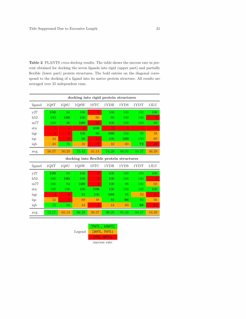
Table 2 presents the results for docking the ligands into rigid (upper

part) and flexible protein structures (lower part). For the docking into rigid

protein structures, it can be observed that all ligands can be docked back

correctly into their native protein structures (bold entries) with high success

rates. As already expected, ligand staurosporine (stu) is docked correctly

into its native protein structure (PDB entry 1STC), but it is docked incor-

rectly in all others. On average, the protein structures of PDB-entries 1JLU

(apo form of PKA), 1Q8T, 1Q8U and 1STC perform worst with respect to

their ability to reproduce the ligand poses correctly with success rates be-

tween 41% and 56%. In contrast, the protein structures of 1Q8W, 1YDR,

1YDS and 1YDT are able to reproduce the correct conformations for all lig-

ands except ligand staurosporine with average success rates of about 74%

to 80%.


Table 2 PLANTS cross-docking results. The table shows the success rate in per-

cent obtained for docking the seven ligands into rigid (upper part) and partially

flexible (lower part) protein structures. The bold entries on the diagonal corre-

spond to the docking of a ligand into its native protein structure. All results are

averaged over 25 independent runs.

docking into rigid protein structures

ligand 1Q8T 1Q8U 1Q8W 1STC 1YDR 1YDS 1YDT 1JLU

y27 100 80 100 0 100 100 100 100

h52 100 100 100 60 88 100 100 8

m77 100 96 100 20 100 100 100 88

stu 0 0 0 100 0 0 0 0

iqp 4 0 100 96 100 100 92 48

iqs 44 0 96 12 100 100 100 60

iqb 48 76 32 0 32 60 72 20

avg. 56.57 50.29 75.43 41.14 74.29 80.00 80.57 46.29

docking into flexible protein structures

ligand 1Q8T 1Q8U 1Q8W 1STC 1YDR 1YDS 1YDT 1JLU

y27 100 88 100 0 100 100 100 100

h52 100 100 100 0 100 100 100 8

m77 100 84 100 4 100 96 100 68

stu 100 100 100 100 100 100 100 100

iqp 4 0 92 100 100 88 52 24

iqs 32 0 68 48 88 96 80 56

iqb 72 84 44 4 44 60 88 24

avg. 72.57 65.14 86.29 36.57 90.29 91.43 88.57 54.29

[70% , 100%]

Legend [30%, 70%)

[0%, 30%)

success rate


In the case of side-chain flexibility, the poses of all ligands can still be

reproduced correctly in their native protein structures (bold entries). Only

the success rate for docking ligand iqs back into its native protein structure

(PDB-entries 1YDS) is insignificantly lowered when compared to the dock-

ing into the rigid protein structure. Ligand staurosporine clearly benefits

from the protein flexibility as the correct pose can be reproduced for all

protein structures now. In fact, flexibility leads to generally higher average

success rates for each protein structure, except for the protein structure of

PDB-entry 1STC. However, for various combinations of proteins and lig-

ands in this experiment, the success rates observed are slightly worse than

in the case when the protein is held rigid. (This lower success rate can be

explained by the extended complexity of the problem and by inaccuracies

in the intra-protein scoring function, which has to score the interactions

arising between the flexible side-chain and the rigid part of the protein cor-

rectly. In the flexible protein side-chain case, the position of this side-chain

needs to be correctly identified by the algorithm—in the rigid case this

side-chain is already in a reasonably good position with respect to the lig-

and, with the main exception being for ligand staurosporine, as explained

above.) Despite this fact, it is a very noteworthy result that the treatment

of protein side-chain flexibility is useful to allow for a better reproduction

of the correct ligand poses. In fact, for four out of eight protein structures

(PDB-entries 1Q8W, 1YDR, 1YDS and 1YDT) we were able to reproduce

the poses of ligands inside 2.5 A of the superimposed crystal structures with

average success rates ranging from about 86% to 91%.

6.2 Virtual Screening

In a next step, the influence of protein flexibility has been investigated in

the context of virtual screening. The virtual screening of large compound

libraries is one of the main applications of current docking tools. Therefore,

PLANTS was also tested with respect to its ability to discriminate between

biologically active and inactive ligands. The best-performing protein struc-

tures identified in the cross-docking of protein kinase A (PDB-entries 1Q8W,

1YDR, 1YDS and 1YDT) have been used as the target structures. The com-

pound library consisted of seven active (the ones already described in the

PKA cross-docking) and 693 supposed inactive ligands. This active/inactive

ratio was chosen, similar to many other virtual screening studies, to simulate

the outcome of a real-world scenario, where usually less than 1 % biolog-


0.5

0.6

0.7

0.8

0.9

1

1YDT1YDS1YDR1Q8W

AU

C v

alu

e

protein structure

rigid protein flexible protein

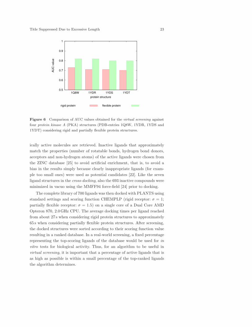
Figure 6 Comparison of AUC values obtained for the virtual screening against

four protein kinase A (PKA) structures (PDB-entries 1Q8W, 1YDR, 1YDS and

1YDT) considering rigid and partially flexible protein structures.

ically active molecules are retrieved. Inactive ligands that approximately

match the properties (number of rotatable bonds, hydrogen bond donors,

acceptors and non-hydrogen atoms) of the active ligands were chosen from

the ZINC database [25] to avoid artificial enrichment, that is, to avoid a

bias in the results simply because clearly inappropriate ligands (for exam-

ple too small ones) were used as potential candidates [22]. Like the seven

ligand structures in the cross-docking, also the 693 inactive compounds were

minimized in vacuo using the MMFF94 force-field [24] prior to docking.

The complete library of 700 ligands was then docked with PLANTS using

standard settings and scoring function CHEMPLP (rigid receptor: σ = 1;

partially flexible receptor: σ = 1.5) on a single core of a Dual Core AMD

Opteron 870, 2.0GHz CPU. The average docking times per ligand reached

from about 27 s when considering rigid protein structures to approximately

65 s when considering partially flexible protein structures. After screening,

the docked structures were sorted according to their scoring function value

resulting in a ranked database. In a real-world screening, a fixed percentage

representing the top-scoring ligands of the database would be used for in

vitro tests for biological activity. Thus, for an algorithm to be useful in

virtual screening, it is important that a percentage of active ligands that is

as high as possible is within a small percentage of the top-ranked ligands

the algorithm determines.


A common measure for evaluating the outcome of a virtual screening

experiment is the area under curve (AUC) value, which is derived from

the receiver operating characteristic (ROC) [26]. Let TP (respectively FP)

be the true (false) positives, that is, the number of ligands selected by the

docking tool that show (do not show) biological activity in in vitro tests,

and FN (resp. TN) be the false (true) negatives, that is, ligands that are

discarded by the docking protocol but show (do not show) biological activity.

Then, the AUC value corresponds to the area under curve when plotting

the false positive rate 1 − sp along the x-axis, where sp = TNFP+TN is also

called the specificity, versus the true positive rate se along the y-axis, where

se = TPTP+FN is the sensitivity. The maximum AUC value reachable is one

and it corresponds to a perfect discrimination between active and inactive

compounds, while AUC values around 0.5 show the performance of random

selection.

The AUC values for all eight virtual screening campaigns are presented

in Figure 6. All four protein structures perform reasonably well in the case

of docking into rigid protein structures with AUC values between 0.7 (PDB-

entry 1YDT) and 0.73 (PDB-entry 1Q8W). An even better discrimination

can be achieved when treating the side-chain of residue PHE327 flexible in

the protein structure as already observed for the cross-docking experiments.

In this case, the protein structures of 1Q8W and 1YDR perform best with

an AUC value of 0.82. However, also for the other protein structures large

improvements for the AUC value can be observed.

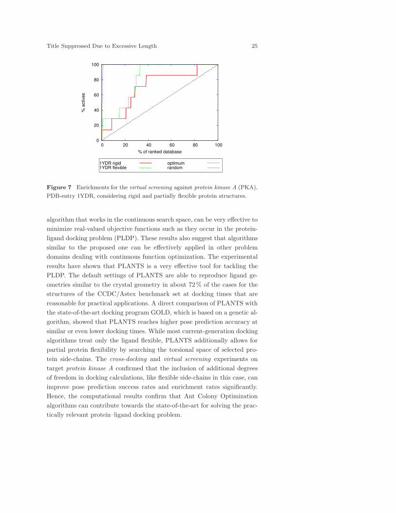
The enrichment curves for the protein structure of 1YDR comparing the

rigid and the flexible case are shown in Figure 7. Both docking protocols

perform clearly better than random selection, but clearly make no optimal

choices. For the rigid case, labeled as 1YDR rigid, the biologically active

ligands can be identified till up to 82% of the ranked database, which is

apparently suboptimal. In contrast, the introduction of protein flexibility

(labeled as 1YDR flexible) allows for the identification of all biologically

active ligands till about 33% of the ranked database, which is also reflected

in the higher AUC value of 0.82.

7 Conclusions

We presented an effective docking algorithm based on the ACO metaheuris-

tic. While most ACO algorithms are designed to tackle discrete optimization

problems, we showed that such an approach, combined with a local search


0

20

40

60

80

100

0 20 40 60 80 100

% a

ctive

s

% of ranked database

1YDR rigid1YDR flexible

optimumrandom

Figure 7 Enrichments for the virtual screening against protein kinase A (PKA),

PDB-entry 1YDR, considering rigid and partially flexible protein structures.

algorithm that works in the continuous search space, can be very effective to

minimize real-valued objective functions such as they occur in the protein-

ligand docking problem (PLDP). These results also suggest that algorithms

similar to the proposed one can be effectively applied in other problem

domains dealing with continuous function optimization. The experimental

results have shown that PLANTS is a very effective tool for tackling the

PLDP. The default settings of PLANTS are able to reproduce ligand ge-

ometries similar to the crystal geometry in about 72% of the cases for the

structures of the CCDC/Astex benchmark set at docking times that are

reasonable for practical applications. A direct comparison of PLANTS with

the state-of-the-art docking program GOLD, which is based on a genetic al-

gorithm, showed that PLANTS reaches higher pose prediction accuracy at

similar or even lower docking times. While most current-generation docking

algorithms treat only the ligand flexible, PLANTS additionally allows for

partial protein flexibility by searching the torsional space of selected pro-

tein side-chains. The cross-docking and virtual screening experiments on

target protein kinase A confirmed that the inclusion of additional degrees

of freedom in docking calculations, like flexible side-chains in this case, can

improve pose prediction success rates and enrichment rates significantly.

Hence, the computational results confirm that Ant Colony Optimization

algorithms can contribute towards the state-of-the-art for solving the prac-

tically relevant protein–ligand docking problem.


There are a number of directions for further research. Of significant sci-

entific interest is certainly a detailed experimental study of the impact of

various components of high-performance docking tools. Most noteworthy are

here the scoring function chosen and the search algorithm chosen. However,

the successful docking tools use a number of problem-specific techniques

that sometimes are not directly transferable when moving from one scoring

function to another or from one search algorithm to another. Hence, such

a study is well beyond the scope of this article and we intend to tackle

this question in future research efforts. Another promising line of research

is the further improvement of scoring functions. Even the best docking al-

gorithms sometimes completely fail on specific target classes, which can in

most cases be attributed to the scoring function. In this context, computa-

tionally more demanding scoring function terms like interactions between

ligands and explicit water molecules are currently under investigation.

An executable version of PLANTS is available on request by contacting

the authors.

Acknowledgments

The authors thank Jens Gimmler and Nicola Zonta for helpful discussions

and a careful reading of the manuscript; they also thank the three anony-

mous referees and the editor-in-chief for the comments that helped to im-

prove the first version of the article. This work was supported by a schol-

arship of the Landesgraduiertenforderung Baden-Wurttemberg awarded to

Oliver Korb. Thomas Stutzle acknowledges support of the Belgian FNRS,

of which he is a research associate.

References

1. G. Muller. Medicinal chemistry of target family-directed masterkeys. Drug

Discovery Today, 8(15):681–691, 2003.

2. H. Berman, J. Westbrook, Z. Feng, G. Gilliland, T. Bhat, H. Weissig,

I. Shindyalov, and P. Bourne. The protein data bank. Nucleic Acids Re-

search, 28:235–242, 2000.

3. Fischer, E. Einfluss der Configuration auf die Wirkung der Enzyme. Chemis-

che Berichte, 27:2985–2993, 1894.

4. D. E. Koshland. Protein shape and biological control. Scientific American,

229(4):52–64, 1973.


5. R. D. Taylor, P. J. Jewsbury, and J. W. Essex. A review of protein-small

molecule docking methods. Journal of Computer-Aided Molecular Design,

16:151–166, 2002.

6. G. Jones, P. Willett, R. C. Glen, A. R. Leach, and R. D. Taylor. Development

and validation of a genetic algorithm for flexible docking. Journal of Molecular

Biology, 267:727–748, 1997.

7. G. M. Morris, D. S. Goodsell, R. S. Halliday, R. Huey, W. E. Hart, R. K.

Belew, and A. J. Olson. Automated docking using a Lamarckian genetic

algorithm and an empirical binding free energy function. Journal of Compu-

tational Chemistry, 19:1639–1662, 1998.

8. R. Abagyan, M. Totrov, and D. Kuznetsov. ICM—A new method for pro-

tein modeling and design: Applications to docking and structure prediction

from the distorted native conformation. Journal of Computational Chemistry,

15(5):488–506, 1994.

9. C. McMartin and R. S. Bohacek. QXP: powerful, rapid computer algorithms

for structure-based drug design. Journal of Computer-Aided Molecular De-

sign, 11(4):333–344, 1997.

10. C. A. Baxter, C. W. Murray, D. E. Clark, D. R. Westhead, and M. D. Eldridge.

Flexible docking using tabu search and an empirical estimate of binding affin-

ity. Proteins, 33:367–382, 1997.

11. E. Kellenberger, J. Rodrigo, P. Muller, and D. Rognan. Comparative evalu-

ation of eight docking tools for docking and virtual screening accuracy. Pro-

teins, 57(2):225–242, 2004.

12. M. Kontoyianni, L. M. McClellan, and G. S. Sokol. Evaluation of docking

performance: Comparative data on docking algorithms. Journal of Medicinal

Chemistry, 47(3):558–565, 2004.

13. T. Stutzle and H. H. Hoos. MAX–MIN Ant System. Future Generation

Computer Systems, 16(8):889–914, 2000.

14. O. Korb, T. Stutzle, and T. E. Exner. PLANTS: Application of Ant Colony

Optimization to Structure-Based Drug Design. In M. Dorigo, L. M. Gam-

bardella, M. Birattari, A. Martinoli, R. Poli, and T. Stutzle, editors, Ant

Colony Optimization and Swarm Intelligence, 5th International Workshop,

ANTS 2006, volume 4150 of Lecture Notes in Computer Science, pages 247–

258. Springer, Berlin, 2006.

15. M. Dorigo and T. Stutzle. Ant Colony Optimization. MIT Press, Cambridge,

MA, USA, 2004.

16. J. A. Nelder and R. Mead. A simplex method for function minimization.

Computer Journal, 7:308–313, 1965.

17. W. H. Press, B. P. Flannery, S. A. Teukolsky, and W. T. Vetterling. Numerical

Recipes in C: The Art of Scientific Computing. Cambridge University Press,

Cambridge, UK, 1992.

18. M. L. Verdonk, J. C. Cole, M. J. Hartshorn, C. W. Murray, and R. D. Taylor.

Improved protein–ligand docking using GOLD. Proteins, 52:609–623, 2003.


19. Gehlhaar, D. K.; Verkhivker, G. M.; Rejto, P. A.; Sherman, C. J.; Fogel,

D. B.; Fogel, L. J.; Freer, S. T. Molecular recognition of the inhibitor AG-

1243 by HIV-1 protease: conformationally flexible docking by evolutionary

programming. Chemistry and Biology, 2:317–324, 1995.

20. Verkhivker, G. M. Computational analysis of ligand binding dynamics at the

intermolecular hot spots with the aid of simulated tempering and binding free

energy calculations. Journal of Molecular Graphics and Modelling, 22:335–

348, 2004.

21. M. Clark, R. D. Cramer III, and N. van Opdenhosch. Validation of the general

purpose tripos 5.2 force field. Journal of Computational Chemistry, 10:982–

1012, 1989.

22. M. L. Verdonk, V. Berdini, M. J. Hartshorn, W. T. M. Mooij, C. W. Murray,

R. D. Taylor, and P. Watson. Virtual screening using protein-ligand docking:

Avoiding artificial enrichment. Journal of Chemical Information and Model-

ing, 44(3):793–806, 2004.

23. J. W. M. Nissink, C. Murray, M. Hartshorn, M. L. Verdonk, J. C. Cole,

and R. Taylor. A new test set for validating predictions of protein-ligand

interaction. Proteins, 49(4):457–471, 2002.

24. T. A. Halgren. Merck molecular force field. I. basis, form, scope, parameteri-

zation, and performance of MMFF94. Journal of Computational Chemistry,

17(5–6):490–519, 1996.

25. J. J. Irwin and B. K. Shoichet. ZINC—A free database of commercially

available compounds for virtual screening. Journal of Chemical Information

and Modeling, 45(1):177–82, 2005.

26. N. Triballeau, F. Acher, I. Brabet, J.-P. Pin, and H.-O. Bertrand. Virtual

screening workflow development guided by the “receiver operating characteris-

tic” curve approach. Application to high-throughput docking on metabotropic

glutamate receptor subtype 4. Journal of Medicinal Chemistry, 48(7):2534–

2547, 2005.

Date post:	19-May-2018
Category:	Documents
Upload:	buithu
View:	215 times
Download:	0 times

An Ant Colony Optimization Approach to Flexible...

Documents