AN APPLICATION OF ANTI-OPTIMIZATION IN THE …mason/Mason_f/JRC_PhD_V2.pdfAN APPLICATION OF...

AN APPLICATION OF ANTI-OPTIMIZATION IN THEPROCESS OF VALIDATING AERODYNAMIC CODES

By

Juan R. Cruz

A DISSERTATION SUBMITTED TO THE FACULTY OF THEVIRGINIA POLYTECHNIC INSTITUTE AND STATE UNIVERSITY

IN PARTIAL FULFILLMENT OF THE REQUIREMENTS FOR THE DEGREE OFDOCTOR OF PHILOSOPHY

INAEROSPACE ENGINEERING

William H. Mason, Chairman Raphael T. Haftka, Chairman

Bernard M. Grossman Elaine P. Scott

Eric R. Johnson

April 4, 2003Blacksburg, Virginia

Keywords: anti-optimization, analysis validation, design of experiments,aerodynamics, wind tunnel testing, Mars airplanes

AN APPLICATION OF ANTI-OPTIMIZATION IN THEPROCESS OF VALIDATING AERODYNAMIC CODES

By

Juan R. Cruz

Committee Chairmen: William H. Mason and Raphael T. HaftkaAerospace Engineering

(ABSTRACT)

An investigation was conducted to assess the usefulness of anti-optimization in theprocess of validating of aerodynamic codes. Anti-optimization is defined here as theintentional search for regions where the computational and experimental results disagree.Maximizing such disagreements can be a useful tool in uncovering errors and/orweaknesses in both analyses and experiments.

The codes chosen for this investigation were an airfoil code and a lifting line codeused together as an analysis to predict three-dimensional wing aerodynamic coefficients.The parameter of interest was the maximum lift coefficient of the three-dimensionalwing, CL max. The test domain encompassed Mach numbers from 0.3 to 0.8, and Reynoldsnumbers from 25,000 to 250,000.

A simple rectangular wing was designed for the experiment. A wind tunnel model ofthis wing was built and tested in the NASA Langley Transonic Dynamics Tunnel.Selection of the test conditions (i.e., Mach and Reynolds numbers) were made byapplying the techniques of response surface methodology and considerations involvingthe predicted experimental uncertainty. The test was planned and executed in twophases. In the first phase runs were conducted at the pre-planned test conditions. Basedon these results additional runs were conducted in areas where significant differences inCL max were observed between the computational results and the experiment – in essenceapplying the concept of anti-optimization. These additional runs were used to verify thedifferences in CL max and assess the extent of the region where these differences occurred.

The results of the experiment showed that the analysis was capable of predictingCL max to within 0.05 over most of the test domain. The application of anti-optimization

iii

succeeded in identifying a region where the computational and experimental values ofCL max differed by more than 0.05, demonstrating the usefulness of anti-optimization inprocess of validating aerodynamic codes. This region was centered at a Mach number of0.55 and a Reynolds number of 34,000. Including considerations of the uncertainties inthe computational and experimental results confirmed that the disagreement was real andnot an artifact of the uncertainties.

iv

Dedication

A mi tía Irma, con amor, cariño, y gratitud.

v

Acknowledgements

I would like to thank all the members of my dissertation committee for their help andadvice. I am especially grateful for the opportunity to have worked with, and learnedfrom, Dr. Haftka and Dr. Mason. Without their guidance and patience this dissertationwould not have been possible.

Two individuals at NASA Langley were key in starting and completing this degree.James Starnes provided the key encouragement to start. Mark Saunders made it possiblefor me to complete it. To both of them I am extremely grateful.

Time is a most valuable asset in a project like this. I thank the following individualsat NASA for making it available to me: Glenn Taylor, Rob Calloway, Mary KaeLockwood, Robert Braun, and James Corliss.

Numerous other individuals at NASA helped in one way or another with the researchpresented here. I am particularly grateful for the assistance rendered by Donald Keller,Mark Guynn, Richard Re, Richard Campbell, and Catherine McGinley. The engineeringand technical staff at the NASA Langley Transonic Dynamics Tunnel were key to thesuccess of the experiment. As with many other projects, the staff at the NASA LangleyTechnical Library were an invaluable resource. Terry Hertz at NASA Headquartersprovided funding that made this research possible. Thanks to all of you.

The support of NASA is also gratefully acknowledged.

Without good friends to provide support and encouragement completing thisdissertation would not have been possible. Thank you Debbie for providing the above aswell as making “Camp Dissertation” available. Michael and Jenny: trials andtribulations of all sorts come through, and you have always been there to help me copewith them. Thanks for listening Dannie. Kate and Drew: thank you for being therethrough lift and sink. The preliminaries and qualifiers were a long time ago, but I stillremember your help Dianne.

vi

Table of Contents

Dedication …………………………………………………………………………… iv

Acknowledgements ..……………………………………………………………… v

Table of Contents ……………………………………………………………….… vi

List of Tables ……………………………………………………………………… ix

List of Figures ……………………………………………………………………… xii

Symbols ….………………………………………………………………………… xvi

Acronyms …………………………………………………………………………… xxiv

Chapter 1: Introduction ….……………………………………………………… 11.1 Motivation …….………………………………………………………… 11.2 Objectives ………………………………………………………………… 21.3 Approach ………………………………………………………………… 21.4 Outline …………………………………………………………………… 5

Chapter 2: Literature Review …………………………………………………… 82.1 Response Surface Methodology ………………………………………… 82.2 Design of Experiments …………………………………………………… 102.3 Experimental Optimization ……………………………………………… 112.4 Model Discrimination …………………………………………………… 122.5 Verification and Validation of Aerodynamic Codes ……………………… 132.6 Concluding Remarks ……………………………………………………… 17

Chapter 3: Aerodynamic Codes and Analysis …………………………………… 183.1 Two-Dimensional Airfoil Code …………….…………………………… 203.2 Lifting Line Theory Code…………….…………………………………… 213.3 Convergence Studies ……………………………………………………… 233.4 Sensitivity of CL max to Ncrit ………………………………………………… 253.5 Uncertainty in the Aerodynamic Analysis Results ……………………… 25

vii

Chapter 4: Experiment Design …………………………………………………… 404.1 Wing Design ……………………………………………………………… 404.2 Test Design Space ………………………………………………………… 414.3 Precision Uncertainty Structure ….……………………………………… 42

4.3.1 Precision Uncertainty Structure of the Maximum Lift Coefficient… 434.3.2 Precision Uncertainty Structure of the Maximum Lift Force ……… 44

4.4 Test Design Analyses and Procedure …………………………………… 444.4.1 Normalization of Dynamic Pressure and Lift ….………………… 454.4.2 Estimation of PL max ………………………………………………… 464.4.3 Response Surface Uncertainty Analysis ….……………………… 494.4.4 Test Design Procedure …………………………………………… 51

4.5 Test Design and Planned Testing Sequence ……………………………… 544.6 A Note on the Bias Uncertainty ………………………………………… 56

Chapter 5: Test Setup and Operations…………………………………………… 675.1 Wind Tunnel Model ……………………………………………………… 675.2 Wind Tunnel Balance …………………………………………………… 695.3 Wind Tunnel ……………………………………………………………… 705.4 Wind Tunnel Test Setup ………………………………………………… 715.5 Test Operations …………………………………………………………… 725.6 Data Acquired …………………………………………………………… 76

Chapter 6: Experimental Data Analyses ………………………………………… 906.1 Wind Tunnel Operating Parameters ……………………………………… 906.2 Forces, Moments, and Nondimensional Aerodynamic Coefficients …… 916.3 Maximum Lift Coefficients ……………………………………………… 936.4 Uncertainties in the Maximum Lift Coefficients ………………………… 96

Chapter 7: Experimental Test Results, Analyses Results, and ComparisonsBetween the Two Sets ………………………………………………… 108

7.1 Experimental Test Results ……………………………………………… 1087.2 Analyses Results ………………………………………………………… 1097.3 Comparison of the Experimental Test Results Against the Analyses

Results …………………………………………………………………… 110

Chapter 8: Conclusions and Observations ……………………………………… 122

References ………………………………………………………………………… 127

Appendix A: Wind Tunnel Turbulence and Ncrit ………………………………… 135

viii

Appendix B: MASC1 Airfoil Nondimensional Coordinates ………………… 140

Appendix C: Wind Tunnel Model Drawings ………………………………… 143

Appendix D: Experimental Data and Analyses Results ……………………… 147

Vita ………………………………………………………………………………… 199

ix

List of Tables

3.1 Convergence studies points …………………………………………… 273.2 Values of CL max for Ncrit = 155 and the range of CL max at the convergence

studies points for the MSES convergence study ……………………… 273.3 Values of Ncrit at the convergence studies points ……………………… 283.4 Sensitivity of CL max to Ncrit at the convergence studies points ………… 283.5 Comparison of the range of CL max from the MSES convergence study

and the Ncrit sensitivity study at the convergence studies points ……… 29

4.1 Values of constants used for fluid properties …………………………… 574.2 Pre-test precision uncertainty estimates for NF, AF, α, p0, p, and T0 at

the one-sigma level……………………………………………………… 574.3 Pre-test aerodynamic analyses results ………………………………… 584.4 Evaluation of PL max as a function of M and Re ………………………… 594.5 Pre-selected test points ………………………………………………… 604.6 Minimum precision error test design …………………………………… 604.7 D-optimal test design …………………………………………………… 614.8 Final test design ………………………………………………………… 614.9 Planned test conditions and run schedule ……………………………… 62

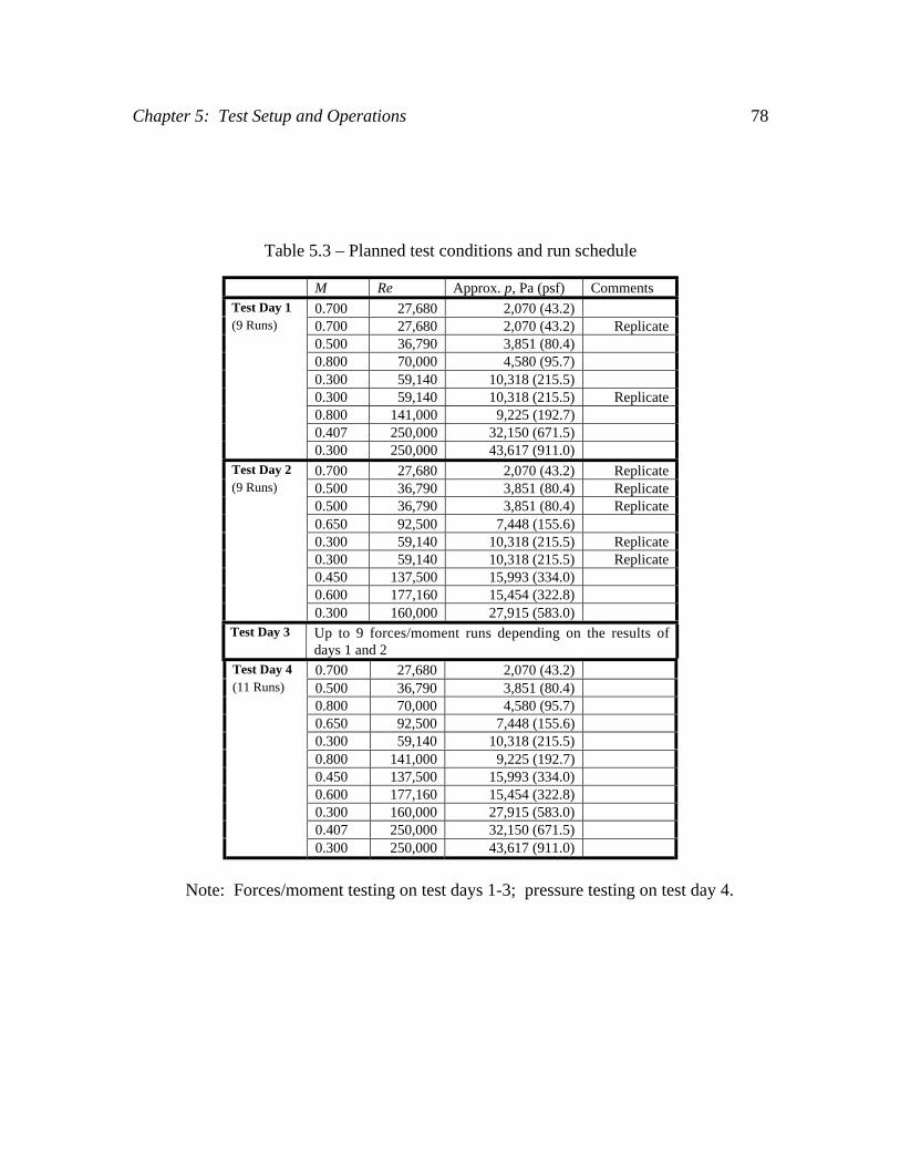
5.1 Key wind tunnel model parameters …………………………………… 775.2 Values of KNF and KPM for the forces/moment and pressures test setups 775.3 Planned test conditions and run schedule ……………………………… 785.4 Actual test conditions and run schedule ………………………………… 795.5 Data acquired during forces/moment testing …………………………… 815.6 Data acquired during pressure testing ………………………………… 81

6.1 Pressure and forces/moment runs correspondence for base pressurecorrection ……………………………………………………………… 99

6.2 Lift curve type for forces/moment runs ………………………………… 1006.3 Example choice of CL max, tab point, M, Re, and α for a Type I lift curve

(Run 15) ………………………………………………………………… 1016.4 Example choice of CL max, tab point, M, Re, and α for a Type II lift

curve (Run 11) ………………………………………………………… 101

x

6.5 Example choice of CL max, tab point, M, Re, and α for a Type III liftcurve (Run 10)…………………………………………………………… 102

6.6 Coefficient values for the CL max response surface in equation 6.23 …… 1026.7 sNF for all tab points identified with CL max……………………………… 1036.8 Sample standard deviation of CL max adj , sCL max

, for nominal conditionswith three or more runs ………………………………………………… 104

6.9 Estimates of the bias uncertainty for NF, AF, α, p0, p, c, and b at the1 – ν = 0.95 (i.e., two-sigma) confidence level ………………………… 104

7.1 Summary of experimental data ………………………………………… 1157.2 Summary of the uncertainty in the experimental data ………………… 1167.3 Summary of aerodynamic analyses results …………………………… 1177.4 Comparison of experimental and analysis results for CL max …………… 118

A.1 Turbulence intensity data and calculated values of Ncrit ………………… 137A.2 Values of the coefficients in the response surface for Ncrit ……………… 137A.3 Comparison of Ncrit values ……………………………………………… 138

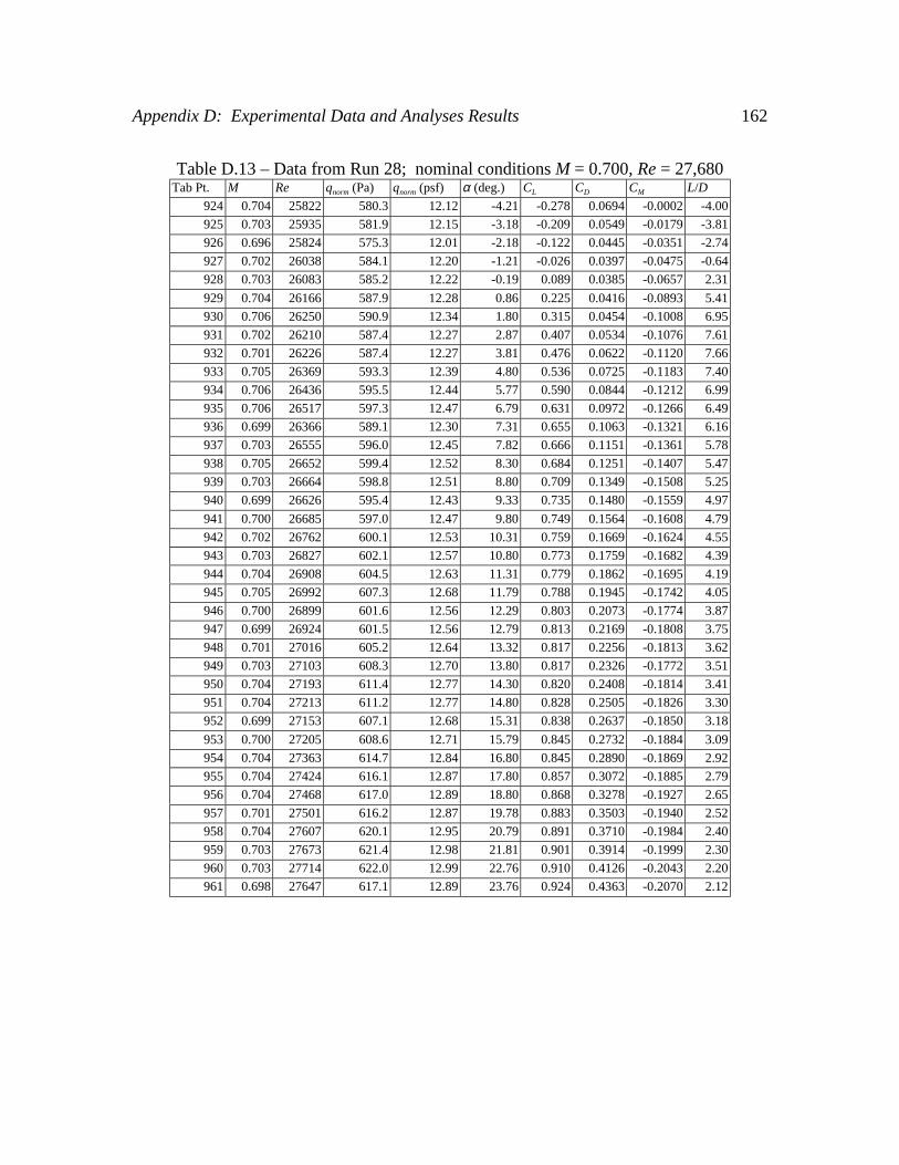
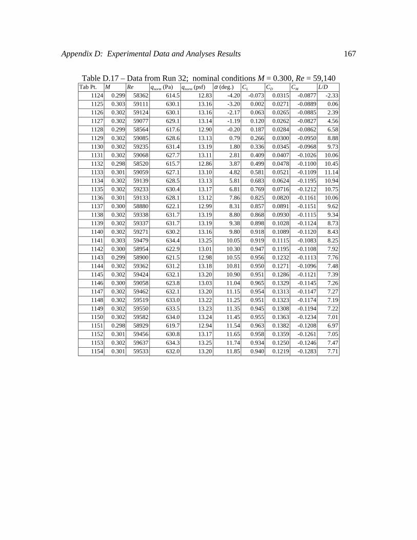
B.1 MASC1 airfoil nondimensional coordinates …………………………… 140

D.1 Data from Run 10; nominal conditions M = 0.800, Re = 70,000 ……… 147D.2 Data from Run 11; nominal conditions M = 0.300, Re = 59,140 ……… 148D.3 Data from Run 12; nominal conditions M = 0.300, Re = 59,140 ……… 149D.4 Data from Run 14; nominal conditions M = 0.800, Re = 141,000 …… 150D.5 Data from Run 15; nominal conditions M = 0.407, Re = 250,712 …… 151D.6 Data from Run 16; nominal conditions M = 0.301, Re = 249,123 …… 152D.7 Data from Run 20; nominal conditions M = 0.700, Re = 27,680 …… 154D.8 Data from Run 23; nominal conditions M = 0.800, Re = 24,584 ……… 155D.9 Data from Run 24; nominal conditions M = 0.700, Re = 27,680 ……… 156D.10 Data from Run 25; nominal conditions M = 0.500, Re = 36,790 ……… 157D.11 Data from Run 26; nominal conditions M = 0.500, Re = 36,790 ……… 159D.12 Data from Run 27; nominal conditions M = 0.800, Re = 70,000 ……… 161D.13 Data from Run 28; nominal conditions M = 0.700, Re = 27,680 ……… 162D.14 Data from Run 29; nominal conditions M = 0.500, Re = 36,790 ……… 163D.15 Data from Run 30; nominal conditions M = 0.651, Re = 92,327 ……… 165D.16 Data from Run 31; nominal conditions M = 0.300, Re = 59,140 ……… 166D.17 Data from Run 32; nominal conditions M = 0.300, Re = 59,140 ……… 167D.18 Data from Run 33; nominal conditions M = 0.451, Re = 138,206 …… 168D.19 Data from Run 35; nominal conditions M = 0.300, Re = 59,140 ……… 169D.20 Data from Run 36; nominal conditions M = 0.599, Re = 176,488 …… 170

xi

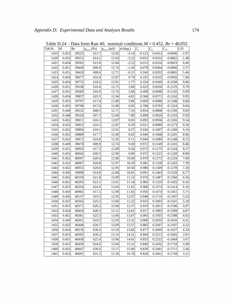
D.21 Data from Run 37; nominal conditions M = 0.300, Re = 160,000 …… 171D.22 Data from Run 38; nominal conditions M = 0.551, Re = 33,521 ……… 172D.23 Data from Run 39; nominal conditions M = 0.500, Re = 36,790 ……… 173D.24 Data from Run 40; nominal conditions M = 0.452, Re = 40,055 ……… 174D.25 Data from Run 41; nominal conditions M = 0.501, Re = 69,870 ……… 175D.26 Data from Run 42; nominal conditions M = 0.550, Re = 90,900 ……… 176D.27 Data from Run 43; nominal conditions M = 0.450, Re = 92,088 ……… 177D.28 Data from Run 45; nominal conditions M = 0.800, Re = 70,000 ……… 178D.29 Data from Run 46; nominal conditions M = 0.800, Re = 141,000 …… 180D.30 Data from Run 47; nominal conditions M = 0.300, Re = 160,000 …… 181

xii

List of Figures

1.1 Mars airplane concept of operations; graphics courtesy of the AresProject, NASA Langley Research Center ……………………………… 7

3.1 cl vs α curve for M = 0.800, Re = 141,000, generated by MSESshowing interpolated region …………………………………………… 30

3.2 Test design space and location of convergence studies points ………… 303.3 CL vs α curve for M = 0.800, Re = 141,000, showing the definition of

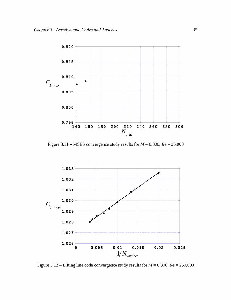
the engineering value of CL max ………………………………………… 313.4 MSES convergence study results for M = 0.300, Re = 250,000 ……… 313.5 MSES convergence study results for M = 0.300, Re = 59,140 ………… 323.6 MSES convergence study results for M = 0.407, Re = 250,000 ……… 323.7 MSES convergence study results for M = 0.550, Re = 137,500 ……… 333.8 MSES convergence study results for M = 0.600, Re = 177,160 ……… 333.9 MSES convergence study results for M = 0.600, Re = 31,410 ………… 343.10 MSES convergence study results for M = 0.800, Re = 141,000 ……… 343.11 MSES convergence study results for M = 0.800, Re = 25,000 ………… 353.12 Lifting line code convergence study results for M = 0.300,

Re = 250,000 …………………………………………………………… 353.13 Lifting line code convergence study results for M = 0.300, Re = 59,140 363.14 Lifting line code convergence study results for M = 0.407,

Re = 250,000 …………………………………………………………… 363.15 Lifting line code convergence study results for M = 0.550,

Re = 137,500 …………………………………………………………… 373.16 Lifting line code convergence study results for M = 0.600,

Re = 177,160 …………………………………………………………… 373.17 Lifting line code convergence study results for M = 0.600, Re = 31,410 383.18 Lifting line code convergence study results for M = 0.800,

Re = 141,000 …………………………………………………………… 383.19 Lifting line code convergence study results for M = 0.800, Re = 25,000 39

4.1 Mars airplane design (top view) showing wing planform. Adaptedfrom figure 2 of reference 4.1. ………………………………………… 63

4.2 Test design space ……………………………………………………… 634.3 Conditions used for pre-test aerodynamic analyses …………………… 64

xiii

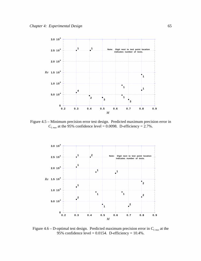
4.4 Aerodynamic analysis CL vs α for M = 0.800, Re = 25,000 …………… 644.5 Minimum precision error test design. Predicted maximum precision

error in CL max at the 95% confidence level = 0.0098.D-efficiency = 2.7%. …………………………………………………… 65

4.6 D-optimal test design. Predicted maximum precision error in CL max atthe 95% confidence level = 0.0154. D-efficiency = 10.4%. …………… 65

4.7 Final test design. Predicted maximum precision error in CL max at the95% confidence level = 0.0116. D-efficiency = 8.2%. ………………… 66

5.1 MASC1 airfoil with zero and finite trailing edge thickness; verticalaxis exaggerated for clarity …………………………………………… 82

5.2 Wing tunnel model assembly with key design dimensions noted ……… 825.3a Wing and balance block assembly, top view, disassembled …………… 835.3b Wing and balance block assembly, bottom view, disassembled ……… 835.3c Wing and balance block assembly, bottom view, assembled, including

wind tunnel balance UT-61A and windshield ………………………… 835.4 Model in wind tunnel showing attachment of windshield to sting …… 845.5 Wind tunnel model components………………………………………… 845.6 Drawing of NASA LaRC wind tunnel balance UT-61A ……………… 855.7 Photograph of NASA LaRC wind tunnel balance UT-61A …………… 855.8 NASA LaRC Transonic Dynamics Tunnel (TDT) aerial view ………… 865.9 TDT operating envelope in air; upper bound adapted from reference

5.4, figure 1(a) ………………………………………………………… 865.10 TDT schematic drawing ………………………………………………… 875.11 TDT sting with the Mars airplane wing ………………………………… 875.12 Pumping time required to achieve low pressures in the TDT ………… 885.13 Model installation, view from below …………………………………… 885.14 Model installation, side view …………………………………………… 895.15 Actual test conditions; digit next to symbol indicates number of tests … 89

6.1 Definition of xbar and ybar and sign convention for NF, AF, and PMbmc 1056.2 Lift curve Type (I, II, or III) as a function of M and Re………………… 1056.3 Example of a Type I lift curve (Run 15) ……………………………… 1066.4 Example of a Type II lift curve (Run 11) ……………………………… 1066.5 Example of a Type III lift curve (Run 10) ……………………………… 107

7.1 Contour plot of |E|, a measure of the difference between theexperimental and analysis values of CL max over the test domain ……… 119

7.2 CL and CM vs α; nominal conditions M = 0.800, Re = 24,584 ………… 1197.3 CL and CM vs α; nominal conditions M = 0.551, Re = 33,521 ………… 1207.4 CL and CM vs α; nominal conditions M = 0.800, Re = 70,000 ………… 120

xiv

7.5 CL and CM vs α; nominal conditions M = 0.700, Re = 27,680 ………… 1217.6 Contour plot using |E| for all conditions with Type I and II CL vs α

curves and |Ealt| for all conditions with Type III CL vs α curves:measures of the difference between the experimental and analysisvalues of CL max over the test domain …………………………………… 121

A.1 Available turbulence data and test design space ……………………… 139

C.1 Drawing 1158620, test wing assembly ………………………………… 143C.2 Drawing 1158621, test wing …………………………………………… 144C.3 Drawing 1158622, balance block and balance roll pin ………………… 145C.4 Drawing 1158623, sting adapter ……………………………………… 146

D.1 CL and CM vs α; nominal conditions M = 0.301, Re = 249,123………… 182D.2 CL vs CD; nominal conditions M = 0.301, Re = 249,123 ……………… 182D.3 CL and CM vs α; nominal conditions M = 0.300, Re = 160,000………… 183D.4 CL vs CD; nominal conditions M = 0.300, Re = 160,000 ……………… 183D.5 CL and CM vs α; nominal conditions M = 0.300, Re = 59,140 ………… 184D.6 CL vs CD; nominal conditions M = 0.300, Re = 59,140 ………………… 184D.7 CL and CM vs α; nominal conditions M = 0.407, Re = 250,712………… 185D.8 CL vs CD; nominal conditions M = 0.407, Re = 250,712 ……………… 185D.9 CL and CM vs α; nominal conditions M = 0.451, Re = 138,206………… 186D.10 CL vs CD; nominal conditions M = 0.451, Re = 138,206 ……………… 186D.11 CL and CM vs α; nominal conditions M = 0.450, Re = 92,088 ………… 187D.12 CL vs CD; nominal conditions M = 0.450, Re = 92,088 ………………… 187D.13 CL and CM vs α; nominal conditions M = 0.452, Re = 40,055 ………… 188D.14 CL vs CD; nominal conditions M = 0.452, Re = 40,055 ………………… 188D.15 CL and CM vs α; nominal conditions M = 0.501, Re = 69,870 ………… 189D.16 CL vs CD; nominal conditions M = 0.501, Re = 69,870 ………………… 189D.17 CL and CM vs α; nominal conditions M = 0.500, Re = 36,790 ………… 190D.18 CL vs CD; nominal conditions M = 0.500, Re = 36,790 ………………… 190D.19 CL and CM vs α; nominal conditions M = 0.550, Re = 90,900 ………… 191D.20 CL vs CD; nominal conditions M = 0.550, Re = 90,900 ………………… 191D.21 CL and CM vs α; nominal conditions M = 0.551, Re = 33,521 ………… 192D.22 CL vs CD; nominal conditions M = 0.551, Re = 33,521 ………………… 192D.23 CL and CM vs α; nominal conditions M = 0.599, Re = 176,488………… 193D.24 CL vs CD; nominal conditions M = 0.599, Re = 176,488 ……………… 193D.25 CL and CM vs α; nominal conditions M = 0.651, Re = 92,327 ………… 194D.26 CL vs CD; nominal conditions M = 0.651, Re = 92,327 ………………… 194D.27 CL and CM vs α; nominal conditions M = 0.700, Re = 27,680 ………… 195

xv

D.28 CL vs CD; nominal conditions M = 0.700, Re = 27,680 ………………… 195D.29 CL and CM vs α; nominal conditions M = 0.800, Re = 141,000………… 196D.30 CL vs CD; nominal conditions M = 0.800, Re = 141,000 ……………… 196D.31 CL and CM vs α; nominal conditions M = 0.800, Re = 70,000 ………… 197D.32 CL vs CD; nominal conditions M = 0.800, Re = 70,000 ………………… 197D.33 CL and CM vs α; nominal conditions M = 0.800, Re = 24,584 ………… 198D.34 CL vs CD; nominal conditions M = 0.800, Re = 24,584 ………………… 198

xvi

Symbols

a speed of sound

Abase model base area

AF axial force

AFcorr axial force corrected for base pressures

AFnorm normalized axial force

AR wing aspect ratio

b wing span

b bM0 , , coefficients in the response surface model for Ncrit

b bRe M Re, ,b

Re2

vb vector of coefficients for the response surface model of L̂norm max

BAF,1−ν bias uncertainty of AF at the 1 – ν confidence level

Bb,1−ν bias uncertainty of b at the 1 – ν confidence level

Bc,1−ν bias uncertainty of c at the 1 – ν confidence level

BNF,1−ν bias uncertainty of NF at the 1 – ν confidence level

Bp,1−ν bias uncertainty of p at the 1 – ν confidence level

Bp0 1, −ν bias uncertainty of p0 at the 1 – ν confidence level

xvii

Bα ν,1− bias uncertainty of α at the 1 – ν confidence level

BCL max ,1−ν bias uncertainty of CL max

BCL max ,1−ν bias uncertainty of CL max adj at the 1 – ν confidence level

c wing chord

cd airfoil section drag coefficient

cl airfoil section lift coefficient

cl max airfoil section maximum lift coefficient

clαairfoil section lift curve slope

cm c/4 airfoil section pitching moment coefficient about the quarter-chord

CA axial force coefficient

Cbase base pressure correction coefficient

CD wing drag coefficient

CL wing lift coefficient

CL max wing maximum lift coefficient

CL max adj maximum lift coefficient adjusted to the nominal values of M and Re

CL max adj mean value of the maximum lift coefficient adjusted to the nominal values of

M and Re

CL max RS maximum lift coefficient response surface as a function of M and Re

CL maxAnalysis maximum lift coefficient from aerodynamic analysis

CM wing pitching moment coefficient about the quarter chord

CN normal force coefficient

xviii

Dnorm normalized drag force

E difference between the experimental and analysis values of CL max

|Ealt| alternate difference between the experimental and analysis values of CL max

EL lower bound of the 95 percent confidence interval of E

Ep percent difference between the experimental and analysis values of CL max

EU upper bound of the 95 percent confidence interval of E

h distance of the flow tangency point aft of the quarter chord

k kM0 , , coefficients in the response surface model for CL max as a function of M and Rek kRe M Re, ,k k

M Re2 2, ,k

M Re2

KNF normal force angle of attack correction factor

KPM pitching moment angle of attack correction factor

Kq normalizing factor for dynamic pressure, forces, and moments

L lift force

Lmax maximum lift force

Lnorm normalized maximum lift force

L̂norm max response surface model for the normalized maximum lift force as a function ofM and Re

L/D lift to drag ratio

M Mach number

n exponent for the determination of the coefficient of viscosity, 0.798803

xix

ne number of elements in the vectors vx and

vb

nobs number of observations used in the creation of the response surface forL̂norm max

Ncrit boundary layer transition turbulence parameter

Ncrit RS Ncrit response surface as a function of M and Re

NF normal force

NFnorm normalized normal force

Ngrid number of grid points on the airfoil surface used in the MSES calculations

Nruns number of runs at a particular test condition

Nvortices number of vortices for the lifting line analysis

p static pressure

pbase1, base pressure at locations 1, 2, and 3, respectivelypbase2,pbase3

p0 stagnation pressure

PAF precision uncertainty of the axial force

PCL maxprecision uncertainty of CL max

PCL max ,1−ν precision uncertainty of the mean of CL max at the 1 – ν confidence level

PL max precision uncertainty of Lmax

PLnorm maxˆ

precision uncertainty of the response surface model L̂norm max

PLmeasprecision uncertainty of the measured lift force

xx

PMbmc pitching moment about the balance moment center

PMbmc corr pitching moment about the balance moment center corrected for basepressures

PMc/4 pitching moment about the airfoil quarter chord

PMc/4 norm normalized pitching moment about the airfoil quarter chord

PNF precision uncertainty of the normal force

Pp precision uncertainty of the static pressure

Pp0precision uncertainty of the stagnation pressure

Pq precision uncertainty of the dynamic pressure

PT0precision uncertainty of the stagnation temperature

Pα precision uncertainty of the angle of attack

q dynamic pressure

qnorm normalized dynamic pressure

R gas constant, 287.05 J/kg K

Re Reynolds number

ℜ 2 coefficient of multiple determination

ℜ adj2 adjusted coefficient of multiple determination

sCL maxsample standard deviation of CL max adj

sNF normal force sample standard error of the mean

S wing area

t airfoil thickness or Student t-Distribution

xxi

T static temperature

TI wind tunnel turbulence intensity

Tref reference value of temperature for the calculation of the coefficient ofviscosity, 300 K

T0 stagnation temperature

T0 ref reference stagnation temperature; 303.8 K for pre-test analyses, 296.1 K forpost-test analyses

t/cmax maximum airfoil thickness to chord ratio

UCAnalysis

L max ,1−ν total uncertainty of CL maxAnalysis at the 1 – ν confidence level

UCL max ,1−ν total uncertainty of the mean of CL max adj at the 1 – ν confidence level

UE, .0 95 uncertainty of E at the 95 percent confidence level

V true airspeed

x airfoil coordinate along chordline

xbar x-component of distance from airfoil quarter chord to the wind tunnel balancemoment center

vx vector of independent variables in the response surface model for L̂norm max

vx0 location vector of independent variables in the response surface model for

L̂norm max

X matrix of observation locations used in the creation of the response surfacemodel for L̂norm max

y airfoil coordinate perpendicular to chordline

ybar y-component of distance from airfoil chordline to the wind tunnel balancecenterline

xxii

ybase y-component offset from the base pressures center of pressure to the windtunnel balance centerline

z percentage point of the standard normal distribution

α angle of attack

α CL max model angle of attack at CL max

α CL max mean value of the model angle of attack at CL max

αs sting angle of attack

α CAnalysis

L maxmodel angle of attack at CL max

Analysis from aerodynamic analysis

β β0 , ,M coefficients for the response surface model of L̂norm max

β βRe M Re, ,β β

M M Re2 2, ,β

M 3

γ ratio of specific heats, 1.399

∆pbase1, differential base pressures at locations 1, 2, and 3, respectively∆pbase2,∆pbase3

∆pwing differential wing surface pressures

µ coefficient of viscosity

µref reference value of the coefficient of viscosity, 1.846 x 10-5 N s/m2

ν tail probability of the standard normal distribution

ρ air density

σ standard deviation of Lnorm max

xxiii

σ̂ estimated value of σ, the standard deviation of Lnorm max

σCL maxstandard deviation of CL max adj

xxiv

Acronyms

AGARD Advisory Group for Aerospace Research and Development

AIAA American Institute of Aeronautics and Astronautics

ATI Advanced Technologies Incorporated

CFD Computational Fluid Dynamics

DAS Data Acquisition System

ISES two-dimensional airfoil code for single-element airfoils

LaRC Langley Research Center

MASC1 Mars Airplane Super Critical #1

MSES two-dimensional airfoil code used in the present investigation; similar toISES but with multiple-element airfoil capability

NASA National Aeronautics and Space Administration

NATO North Atlantic Treaty Organization

RMS Root-Mean-Square

RSM Response Surface Methodology

TDT Transonic Dynamics Tunnel

V&V Verification and Validation

1

Chapter 1: Introduction

1.1 Motivation

Practitioners of design optimization have often observed that optimization algorithmsseem to possess an uncanny ability to exploit weaknesses in the underlying analyses andconstraints. Unger [1, pp. 51-53] presents an example of such behavior. During theoptimization of a wing for a high-speed civil transport the optimization algorithmdetermined that there was an advantage in using a highly swept wing tip to reduce thedrag due to lift. This behavior was deemed unrealistic and was eliminated as a possibleoutcome of the optimization procedure by adding a geometric constraint. In other casessuch behavior identifies errors in the underlying analyses which, once isolated by theoptimization algorithm, can then be corrected. Thus, this “ability” of optimizationalgorithms can sometimes yield useful information.

These observations led to the question: Why not use this behavior of optimizationalgorithms to assist in the process of validating codes and/or analyses1 by helping toidentify weaknesses and errors? This idea was proposed by Haftka and Kao [2], andothers as discussed in the literature review. Pursuing the application and determining theusefulness of this idea to the process of validating aerodynamic analyses2 is the subjectmatter of the present research. To differentiate this use of optimization from otherapplications (e.g., design optimization, optimal design of experiments), the use beingpursued herein will be called anti-optimization - active search for the “worst” behavior.3

Besides identifying weaknesses in analyses, anti-optimization may have other qualitiesthat are useful. It is often difficult to isolate problems with an analysis as compared toanother analysis or experimental data if the differences are small; multiple sources

1 In this work a code is considered to be a single computer program. An analysis is defined here as a singlecode or combination of codes used to yield the output parameter being investigated (e.g., maximum liftcoefficient). In general the term code will be used here to refer to specific computer programs.2 Unless otherwise stated, in the present research validation is used in reference to the ability of an analysisto model physical reality. Verification, on the other hand, is used to describe the ability of a code to solvethe intended governing equations correctly, regardless of the suitability of the governing equations to modelphysical reality. A complete discussion of this terminology is given in the literature review, chapter 2,section 2.5.3 The term anti-optimization was coined by Elishakoff in reference to the search for the “least favorableresponse” [3, 4]. Various researchers have proposed the concept of validating analyses by maximizingdifferences. These works are discussed in the literature review (chapter 2).

Chapter 1: Introduction 2

(e.g., inadequacy of the physical model, convergence problems, coding errors) could bethe reason for small discrepancies. By maximizing the differences, however, it may beeasier to diagnose the reason for the weakness in the analysis. Anti-optimization can beused in the process of validating analyses by either comparing competing models (an areaof study often known as model discrimination), or by seeking discrepancies betweenanalyses and experiments. In the present investigation, the later approach is pursued.

1.2 Objectives

The primary objectives of the work performed for this dissertation are to develop anapproach using anti-optimization in the process of validating aerodynamic analysesthrough experiments, and to evaluate the effectiveness of this approach. Consistent withthe desire to apply optimization as a tool to achieve these objectives, methods from theoptimal design of experiments literature will be utilized. In particular, tools developedfor the statistical design of experiments and response surface methodology [5] will beused. The concept of anti-optimization will be applied to search for regions in which theanalysis and experiment disagree, and to maximize these disagreements.

Since the present research is an applied study, a suitable aerodynamic analysisneeding validation and an appropriate corresponding experiment were selected to serve asa testbed for the approach being developed. A combination of two aerodynamic codesintegrated into an analysis to predict the maximum lift coefficient of a wing and a relatedwind tunnel experiment were chosen to exercise and evaluate the proposed approach. Aninteresting flight domain for the validation of this analysis is the combination of Machand Reynolds numbers encountered by airplanes operating within the atmosphere ofMars. As detailed in the next section, Mars airplanes operate at unusual combinations ofthese parameters. The scarcity of data in this flight domain, the possibility of validatingthe analysis in an efficient manner through the approach proposed herein, and NationalAeronautics and Space Administration (NASA) interest in these data for future Marsmissions, made the experiment of interest in and of itself. Thus, secondary objectives ofthe dissertation were assist in the validation of an analysis in the flight regime used byairplanes designed to fly in the Martian atmosphere, and to generate an aerodynamicsdatabase in this flight regime.

1.3 Approach

Given the research objectives presented in the previous section, the following generalapproach is proposed to fulfill them:

1) Selection of the analysis and output parameter to be validated. In choosing ananalysis and output parameter the capability to perform a suitable experimentshould be kept in mind. For example, if an experiment yielding sufficiently


accurate results is not possible, the prospects of making meaningful comparisonsbetween computational and experimental results is doubtful.

2) Definition of the experiment. The experiment should yield the requiredexperimental data to compare against the results from the analysis. At this stagethe possibility of performing a suitable experiment within the available resourcesshould be evaluated.

3) Generation of preliminary computational results. These preliminarycomputational results will assist in the design of the experiment as describedbelow. In addition, these preliminary computational results can be used toperform real-time comparisons against the experimental results while theexperiment is being executed. Making these comparisons while the test is beingconducted allows on-the-spot changes in the test design as required, especiallysince the goal is to search for regions were the correlation between thecomputational and experimental results is poor.

4) Design of the experiment. In this stage all the details of the experiment that canbe specified before testing starts should be defined. Items that require definitioninclude physical aspects (e.g., models, equipment, facilities) and otherconsiderations such as selection of the experimental test conditions (which maybe done, for example, by formal optimal design of experiments techniques).

5) Execution of the experiment. At this stage the experiment is conducted, guided bythe pre-test planning, but making changes as necessary as experimental results aregenerated.

6) Comparison of experimental and computational results. In comparing theseresults, areas where the computational and experimental results do not agree areisolated. In an additional stage, not included in the present research, a search forthe reasons why the computational and experimental results differ is conducted(i.e., diagnosing problems with the analysis and/or experiment).

7) Generate conclusions. Evaluate how well the general approach proposed herein,and the details of the particular implementation for the validation of experiments,satisfied the objectives of the present investigation.

In subsequent chapters of this dissertation points three through seven above are coveredin detail. However, the choices made with regards to items one and two are discussedhere. To understand the reasons for these choices, a brief description of the operation andchallenges of operating airplanes in the atmosphere of Mars is required.

Over the last 25 years, NASA has investigated the possibility of conducting roboticmissions on Mars using airplanes as the platform for the scientific instruments. One of


the earliest, and yet most thorough, studies was presented in reference 6. In this proposeddesign the airplane concept of operations, shown in figure 1.1, proceeds as follows:

• The airplane is packaged in a folded configuration inside an aeroshell.

• The aeroshell enters the Mars atmosphere and protects the airplane from theheat generated during entry.

• A parachute is deployed at supersonic speeds. This parachute slows theaeroshell to subsonic speeds.

• The heat shield is released, exposing the folded airplane to the airstream.

• The airplane is released from the backshell.

• The airplane unfolds, assembling itself in mid-air.

• The airplane performs a pullout maneuver from its initial steep dive, finallyachieving level flight. Because of the thin Martian atmosphere this pulloutrequires several kilometers of altitude. During the pullout the airplaneaccelerates to transonic Mach numbers.

This Mars airplane concept of operations, although not the only possible option, has beeninvestigated further by other researchers. In reference 7 a detailed entry/descent/flightanalysis was conducted. This analysis included all phases listed above, from the time theaeroshell enters the atmosphere and concluding with the end of the pullout from theinitial dive. Among the key observations made in this reference is that the maximum liftcoefficient of the wing is critical to the success of the pullout maneuver. Airplanes withhigher values of the maximum lift coefficient can accomplish the pullout maneuver withless altitude loss while experiencing a lower maximum Mach number – thus enhancingmission safety. Conversely, higher values of the maximum lift coefficient allow heavierairplanes to perform the pullout maneuver within given altitude loss and maximum Machnumber constraints. This added pullout mass capability can be used to enhance missionvalue by allowing additional scientific instrumentation to be flown. Because of the lowatmospheric density on Mars, the combination of Mach and Reynolds numbers during thepullout of Mars airplanes such as the one described in reference 7 is highly unusual:Mach numbers up to 0.8 and Reynolds numbers as low as 43,000. Thus, during pulloutthis proposed airplane operates in the Mach number regime usually associated withcommercial transports and the Reynolds numbers regime usually associated with birdsand model airplanes. This unusual combination of Mach and Reynolds numbersgenerated concerns regarding the capability of current aerodynamic analyses toaccurately predict wing performance, in particular the maximum lift coefficient.


Validating the ability of an analysis to predict the maximum lift coefficient was aninteresting and attractive option for the research proposed in this dissertation for a varietyof reasons. The problem was naturally constrained to a clearly identifiable responseparameter, namely the maximum lift coefficient that, for a given wing, is only a functionof two independent variables – Mach and Reynolds number. Analyses exist for theprediction of the aerodynamic performance of wings at the required Mach and Reynoldsnumbers, although they had not been validated at the Mach and Reynolds numbercombinations required by Mars airplanes. A wind tunnel that can operate at the requiredtest conditions exists at the NASA Langley Research Center (LaRC), namely theTransonic Dynamics Tunnel. Previous research efforts at NASA LaRC related to Marsairplanes (both computational and experimental) could be used as a starting point for thepresent investigation. Finally, continuing interest at NASA in Mars airplane missionsmade it possible to undertake the required experiment.

The aerodynamic codes chosen for the present investigation were an airfoil code topredict the two-dimensional airfoil properties, and a lifting line code to predict the three-dimensional wing aerodynamic parameters (in particular the maximum lift coefficient)based on the two-dimensional airfoil data. The relative simplicity and speed of executionof these codes made it possible for them to be used for the present investigation. Thecomputational cost of more complex codes (i.e., three-dimensional Navier-Stokes) wouldbe prohibitive. The design of the test wing was influenced by the analyses in reference 7,and previous unpublished experimental work performed at the TDT on the aerodynamicsof Mars airplanes

1.4 Outline

This dissertation is organized as follows:

In chapter 2 a literature review is presented, focusing on the statistical design ofexperiments and the validation of aerodynamic codes through experiments.

In chapter 3 the aerodynamic codes used in the analysis used herein: a two-dimensional airfoil code and a lifting line code, are discussed. Together these two codeswere used to predict the maximum lift coefficient of a three dimensional wing. In thischapter the results of convergence studies are presented. These convergence studies wereconducted to determine appropriate values of discretization variables in the two-dimensional airfoil code and the lifting line code. The sensitivity of the computationalresults to the wind tunnel turbulence was also investigated. As closure to chapter 3, anassessment of the computational aerodynamic results uncertainty is presented.Knowledge of this uncertainty is important when comparing analysis vs experimentalresults.


In chapter 4 the experimental design, including the design of the wing, the definitionof the experimental design space, and the selection of the test conditions based on designof experiments techniques and response surface methodology is presented and discussed.

In chapter 5, the wind tunnel test setup and its operation are discussed. Included inthis discussion are detailed descriptions of the wind tunnel model and balance. Becauseof the unusual test conditions (i.e., high Mach number and low Reynolds numbers) usedduring the present research, the wind tunnel used and how it is operated is relevant to thisdiscussion. Thus the wind tunnel, test setup, and test operations are also presented indetail. Finally the data to be acquired during testing is specified.

In chapter 6 the methodology used to analyze the experimental data is presented.Included are the determination of wind tunnel conditions, forces, moments, andnondimensional aerodynamic coefficients with emphasis on the maximum lift coefficientand its uncertainty.

In chapter 7 the experimental and computational test results, including theiruncertainties, are presented and discussed. The experimental and computational resultsare compared, and areas of disagreement between experiments and computations foundthrough the use of anti-optimization are isolated.

Finally in chapter 8 the conclusions reached at during the present research aresummarized and discussed. Included in these conclusions is an evaluation of thesuitability of the approach implemented to achieve the stated research objectives.


Figure 1.1 – Mars airplane concept of operations; graphics courtesy of the Ares Project,NASA Langley Research Center

8

Chapter 2: Literature Review

Literature relevant to the present investigation can be categorized into the followinggroups:

• Response Surface Methodology• Design of Experiments• Experimental Optimization• Model Discrimination• Verification and Validation of Aerodynamic Codes

Each of these areas will be discussed separately in this literature review. However, itshould be noted that there is significant overlap among them; they should not beconsidered to be completely independent areas of study.

Haftka et al. [8] reviewed the relationship between optimization and experiments. Inthis review paper they divided the topic into four areas:

• Use of optimization for designing experiments• Use of experiments to perform optimization• Use of experimental optimization techniques in numerical optimization• Importance of experimental validation of optimization

Of these four areas, the first two are relevant to the present investigation. This reviewpaper will be used extensively to discuss the first four subjects in the present literaturereview.

2.1 Response Surface Methodology

Response surface methodology (RSM) concerns itself with the creation and analysisof functions to model how some particular quantity (known as the response) varies withrespect to a set of relevant independent variables. Topics usually included within RSMinclude:

• Generation of response functions. Low-level polynomials are commonly, butnot exclusively, used as response functions.

Chapter 2: Literature Review 9

• Fitting experimental and computational data to response surface functions,usually through least-squares procedures.

• Estimation of the values of unknown coefficients in the response function.

• Analysis of uncertainty of both the response surface and the estimates of theparameters in the response function.

• Seeking maximum and minimum values of the fitted response surface.

• The design of optimal experiments where the experimental results are to befitted with a particular response surface. A common example of this is theoptimal design of an experiment to minimize the uncertainty in the responsefunction parameters (e.g., D-optimal designs).

In their 1951 paper, Box and Wilson [9] discussed many of the important aspects ofRSM. Their main goal was to identify the maximum (or minimum) of a responsefunction generated on the basis of experimental data. They achieved this by sequentialexperimentation using previous results to guide the continuing experimental designs. Theresponse surfaces they used were linear in the response variables (i.e., factors); leastsquares were used to determine the unknown coefficients. Box and Wilson alsoidentified lack-of-fit (i.e., bias) in the assumed response function as an area of concern.By the mid 1960s, RSM had been sufficiently developed to warrant a literature reviewpaper by Hill and Hunter [10]. This review paper discusses both the theoretical aspectsof RSM, as well as practical applications in a variety of fields. Another, morecomprehensive, review paper was published by Mead and Pike [11] in 1985. In additionto the usual topics such as response functions, this paper covers D-optimal experimentaldesigns and experimental designs for model discrimination. More recently, RSM hasbeen used to fit response functions to the results of computer analyses. This is notsurprising, since computational results can exhibit two key similarities with physicalexperiments: they can be expensive to perform, and numerical noise can mimicexperimental uncertainty.1 By fitting a simple and computationally inexpensive responsesurface to selected computer analyses, and then using the response surface as a surrogatefor the computer analyses, computational efficiencies can be achieved. This use of RSMis reviewed by Haftka et al. [8]. At the present time, RSM is an established tool to modelboth experimental and computational results, and the subject of recent textbooks andmanuals [5, 12].

1 Although computational results are the same every time a code is executed with identical inputs,converged solutions can yield slightly different results when certain parameters such as the computationalgrid are changed. It is these variations in the computational results that mimic experimental uncertaintyand are referred to as numerical noise.


2.2 Design of Experiments

The term design of experiments, as commonly used, implies the selection of testconditions to achieve some specific goal. Among the goals usually sought in the designof experiments are maximization or minimization of the response (whether this is donevia response surface functions or by other means), minimization of the uncertainty of theresponse function, minimization of the uncertainty of the parameters being identified, andmodel discrimination. The application of design of experiments to model discriminationis particularly relevant to the present investigation, and is discussed separately in asubsequent section. Regardless of the specific goals being sought, most design ofexperiments techniques have one thing in common: maximizing the quality of the dataobtained while minimizing the number of experiments to be conducted.

In an early example, Fisher and MacKenzie [13] report the design, execution, andresults of a planned experiment to determine the response of various potato varieties tomanure. By carefully selection of the planting locations of different varieties, themanurial treatments, and the number of replicates this experiment was able to quantifythe influence of these parameters with statistical confidence. Box and Wilson [9]suggested the use of two-level factorial, fractional factorial, and composite designs forseeking the maxima of a response surface. The properties and usefulness of these designsin RSM are discussed by Myers and Montgomery [5]. Taguchi methods [14] applysimilar orthogonal designs for maximizing responses.

If the goal of the experimental design is identification of the parameters in theresponse surface, a set of optimality criteria based on the Fisher information matrix forthe design of such experiments have been developed [8]. Numerous optimality criteriahave been proposed (e.g., A-, C-, D-, E-, and L-optimality). These are reviewed byWalter and Pronzato [15], and Haftka et al. [8].

Although design of experiment techniques have been used for years in various fields(e.g., chemistry, biology), it is only recently that they have begun to be applied toaerospace wind tunnel testing. DeLoach [16, 17, and 18] has proposed the use of designof experiments and RSM techniques in wind tunnel experiments instead of the commonlyused “one factor at a time” approach. He cites reductions in costs to achieve the desiredobjectives and improvements in precision accuracy as a significant reasons to apply thedesign of experiments approach to wind tunnel testing. In an experiment to quantify thedeformation of a supersonic transport model as a function of angle of attack, Machnumber, and Reynolds number, the designed experiment required 60 percent fewer wind-on minutes than the “one factor at a time” experiment for the same level of accuracy.Landman et al. [19] discuss the results of a designed wind tunnel experiment using RSMtechniques to predict the performance of a racecar. The regression models identifiedinteractions in the lift and lift to drag responses the authors state “would have beenoverlooked in a traditional OFAT (one factor at a time) approach to testing.”


2.3 Experimental Optimization

How experimental optimization can be conducted has already been discussed as itrelates to the design of experiments and RSM. This section focuses on the reasons whyexperimental optimization is pursued. The discussion in this section follows that ofHaftka et al. [8].

Experimental optimization, instead of analytical optimization, is undertaken for avariety of reasons. In the present investigation, experimental optimization is used tomaximize the difference between analysis and experiment, since the goal is to validatethe analysis and the experiment is considered to be the “ground truth.” However, thereare other reasons for pursuing experimental optimization instead of analyticaloptimization. In some cases there are doubts on the reliability of computational models,or no computational model exists. Landman [20] optimized the position of the flap on amulti-element airfoil to yield the maximum lift coefficient. Among the reasons cited byLandman to perform this optimization experimentally was the accuracy limitations ofcurrent computational tools to predict the maximum lift coefficient of such airfoils.

In cases where the response and thus the optimum varies within supposedly identicalsystems, and/or within a given system with time, experimental optimization may be thepreferred approach. Stuckman et al. [21] discuss the experimental optimization of thegains in the control system of a robot to minimize the cycle time to perform certain tasks.By conducting an experimental optimization procedure, Stuckman et al. were able tooptimize the control system gains of a robot to reduce the cycle times for two specifictasks. They note that these optimizations could be conducted again at a later time tore-optimize the system, which would account for wear in the robot’s mechanism.

Experimental optimization is also an attractive option in situations where theexperiments are inexpensive. Process control is an example of such an application.Semones and Lim [22] report on the optimization of the productivity of a yeast culture,where the control variables were the temperature and the dilution rate. The optimizationalgorithm was able to bring the productivity to an optimum steady state value, andrecover from intentional and unintentional disturbances. If the experiment isinexpensive, can be easily performed one at a time, and the noise level is low, slopebased methods from analytical optimization can be used in experimental optimization. Inthe multi-element airfoil study by Landman [20], all these conditions were met. Thus, hewas able to optimize the flap position by using a steepest ascent algorithm. However, inmany experimental optimization situations the noise level is not low, and alternateoptimization algorithms must be used. Spendley et al. [23] proposed the sequential use ofa simplex designs (an equilateral triangle in two dimensions) to seek the experimentaloptimum of a response. Based on three simple rules, this procedure would seek themaximum of an experimental response. The basic idea in two dimensions is thereplacement of the vertex with the lowest response by moving away from it by rotating


the equilateral triangle about the other two vertices. Experimental noise is dealt with byperiodically replacing previous measurements according to specified rules.

2.4 Model Discrimination

The concept of using designed experiments to differentiate between competingmodels is known in the literature as model discrimination. A key element of modeldiscrimination is the maximizing of differences between the competing models. Thus, inprinciple it is similar to the concept of anti-optimization being used herein. This makesthe model discrimination literature of interest to the present investigation. The discussionrelated to model discrimination in this section is adapted from the review by Haftka et al.[8] of which I am a co-author and main contributor to this section.

Optimization can be used to design experiments that will discriminate amongcompeting models of physical phenomena. Hill [24] reviewed proposed experimentaldesign procedures to discriminate among competing models. One of the earliestprocedures reviewed by Hill is that of Hunter and Reiner [25]. The Hunter and Reinerexperimental design procedure is intended to discriminate among two competing models.After an initial set of experiments is completed, the two competing models are fitted tothe experimental data. Additional experimental points are placed at locations where thepredictions of both models differ the most. Doing this intentionally places the models injeopardy, so that one is shown to be more correct than the alternate. By its very naturethis procedure is sequential and requires repeated experimentation. In the presentinvestigation this sequential experimental procedure to maximize differences is namedanti-optimization, and is conducted between a single analysis and a correspondingexperiment. Froment [26] shows how the Hunter and Reiner procedure can be extendedto more than two models.

The Hunter and Reiner procedure is intended to be applied to chemical reactionkinetics, and it is often cited in this literature. However, no references in the chemicalliterature were found of it being used with actual experimental data. A likely reason forthis is the development of a more general procedure, discussed below, by Box and Hill[27]. Nevertheless, the Hunter and Reiner procedure is general and has been applied toother fields. Schmid-Hempel [28] presents an example of its use to discriminate amongtwo models of nectar-collecting by honeybees. It has also been proposed for use in thestudy of water resources by Knopman and Voss [29] and for environmental field studiesby Eberhardt and Thomas [30].

Box and Hill [27] proposed an alternate approach to model discrimination thataddressed two criticisms of the Hunter and Reiner [25] procedure. First, their approachallows for the discrimination among multiple models, not just two. Second, theirapproach allows for consideration of the error of the estimated difference among models.As with the Hunter and Reiner procedure, that proposed by Box and Hill is sequential in


nature. Several applications of the Box and Hill approach appear in the chemistryliterature [31, 32, and 33]. Atkinson [34] compared the Hunter and Reiner and the Boxand Hill procedures for the case of two competing models. In the examples heconsidered, no significant differences were found between the two procedures.

Atkinson [35] proposed a procedure to test the adequacy of a particular model. Themodel under consideration is incremented with additional extension terms with unknowncoefficients. Experimental designs such as D-optimal are then used to defineexperiments to determine the values of all unknown coefficients, including the extensioncoefficients. The suitability of the original model is assessed by testing the significanceof the extension terms. Candas et al. [36] used a variant of Atkinson’s procedure todiscriminate among models for the distribution and metabolism of corticotropin-releasingfactors in rats. The models consisted of sums of exponential terms with unknownparameters (coefficients and exponents). Two models were considered: a biexponential(i.e., two-term) model, and a triexponential (i.e., three-term) model. The biexponentialmodel was contained within the triexponential model. Using a combined sampling set,they determined that the triexponential model produced the best fit to their data. Afeature of this procedure for model discrimination is that, since it is not sequential, it issuited for experiment preferably performed in pre-determined batches.

In the aerospace field, Haftka and Kao [2] suggested the use of numericaloptimization to sharpen the differences between competing models for compositelaminate failure, and using these results to guide subsequent experiments. Wamelen et al.[37] followed through on this suggestion, undertaking the indicated optimization andperforming a set of experiments that validated one of the two competing analyses.

2.5 Verification and Validation of Aerodynamic Codes

Although not all the codes used in the present investigation can be considered to beComputational Fluid Dynamics (CFD) codes, the substantial literature related to theverification and validation (V&V)2 of CFD codes is directly applicable. Thus, theliterature related to V&V of CFD codes is of interest to the present investigation andreviewed in this section.

During the late 1980s it became evident that there was a need for a more formalizedapproach to the verification and validation (V&V) of CFD codes. To satisfy that need,the North Atlantic Treaty Organization’s (NATO) Advisory Group for Aerospace 2 The terms verification and validation have not been used consistently in the literature. In the presentinvestigation verification relates to the numerical correctness of codes, while validation refers to a code’sability to model the physical world. When verification and validation are used with these meanings theyappear in italics within this chapter. The acronym V&V is always used with these meanings. Insubsequent chapters they are always used with these meanings and appear in regular type. Whenverification and validation are used with other meanings by specific authors cited in this literature reviewthey appear in regular type with the meaning given to them by the specific authors.


Research and Development (AGARD) organized a conference in 1988 to discuss V&Vand survey the current thinking and state of the art in this area within the aerospacecommunity. The proceedings of this conference were published in two volumes [38, 39],and evaluated by Sacher et al. in reference 40. Particularly important among the papersof this conference were those in Session I, “CFD Validation Concepts,” by Bradley [41],Marvin [42], and Boerstoel [43] since they set the tone for the work in this area throughthe following decade. Bradley stressed the need for code validation to achieve “MatureCapability” or “Level V” in the five-step CFD development cycle he presents. He usedthe term validation in referring to both verification and validation. Marvin addresses the“role of experiment in the development of Computational Fluid Dynamics (CFD) foraerodynamic flow prediction,” with the key point being that “CFD verification is aconcept that depends on closely coordinated planning between computational andexperimental disciplines” [42, p. 2-1]. With respect to experiments he stresses the needfor completeness and accuracy. Boerstoel stresses the need to assess the numericalaccuracy of the codes (by what he calls numerical experiments), independently ofcomparisons of physical data. These papers thus establish: 1) the need for CFD V&V(Bradley), 2) the importance of verification (Boerstoel), and the role of experiments invalidation (Marvin). Following this conference, significant work in this area wasundertaken. By 1998 CFD code V&V was the subject of a special section in an issue ofthe American Institute of Aeronautics and Astronautics (AIAA) Journal [44], a book byRoache [45], and a set of guidelines by the AIAA [46]. Oberkampf et al. [47] recentlyreviewed the state of the art. At the present, a consensus in the terminology and methodshas evolved, but much work remains to be done. This is stated in the AIAA guide asfollows: “The document’s goal is to provide a foundation for the major issues andconcepts in verification and validation. However, this document does not recommendstandards in these areas because a number of important issues are not yet resolved.” [46,p. i].

As has been noted, the terms verification and validation have been used with differentmeanings and/or interchangeably in the literature. Oberkampf [48] reviewed the termsand definitions used by various authors, and concluded that the definitions forverification and validation proposed by Blottner [49] based on the work of Boehm [50,p. 728] captured the essence of the terms, and clearly separated them so that the activitiesthey imply could be addressed. Blottner defined verification and validation as follows:

Verification: “Code verification (solving governing equations right) is thedetermination of the accuracy of the numerical solution of the chosen governingequations.”

Validation: “Code validation (solving right governing equations) is theevaluation of the accuracy of the governing equations that are being solved.”

(quotations from reference 49, page 113; italics in quotes by the original author.). Theseare essentially the definitions adopted by Roache [45] in his book, and by the AIAA in its


guide [46]. Thus, there is a consensus building around these definitions and they areadopted in the present investigation.

As pointed out by Roache [45] verification is a mathematical exercise and can beundertaken without experimentation. Aeschliman et al. [51] identified the issuespertinent to CFD code verification as falling into one of the following categories:discretization of the continuum equations, spatial and temporal discretizationconvergence, iterative convergence, programming errors, and round-off/truncation errors.Aeschliman and Oberkampf have proposed that comparison with “exact analyticsolutions, computations from previously verified codes, and codes that addresssimplified, or specialized, cases” be used for code verification [52, p. 733]. Roache [53]proposed the Grid Convergence Index method for assessment of the convergence of aCFD code, without having to double the grid density. Once a code is verified, there aresome assurances that the code will converge to a correct solution of the equations used asthe grid density increases. However, even after a code is verified, Roache [53] haspointed out that its use for a particular calculation also needs to be verified to assess theaccuracy for the particular calculation at the specified grid density. A good example ofcalculation verification is given in reference 54 by McWherther Walker and Oberkampf.In this study, designed specifically for code verification and validation, the force andmoment coefficients of a hypersonic vehicle were studied as a function of the number ofstreamwise grid points, circumferential grid points and body to shock grid points.Richardson extrapolation was used to estimate the “‘exact’ solution as the number of gridpoints approaches infinity.” [54, p. 2012]. The convergence criteria used was a onepercent difference between the actual solution and the extrapolated “exact” solution.Based on this criteria, particular values of the streamwise, circumferential, and shock gridpoints were selected for the computations. In order to proceed with validation,verification of the code and the particular calculation, is recommended. This sequentialapproach is advocated by several authors, including Melnik et al. [55, p. 3] and Roache[45, p. 29].

Roache [45, p. 24] has pointed out that the key difference between verification andvalidation is that verification lies in the realm of mathematics, where as validation is partof science and engineering. Thus, validation requires experimentation. In the earlierpapers on this subject the required experimental data was obtained from previouslypublished research [56], existing databases [57, 58], or databases explicitly collected forcode validation [59, 60]. However, existing experimental data and/or data bases wereoften found to be inadequate for CFD code validation. Baltar and Tjonneland [61] notedthat lack of documentation in the existing experimental data they used was of concern.Bertin et al. [62] noted that in their area of interest (sharp cones at hypersonic speeds)“the quality of the data available in the open literature is uneven and, in most cases, noattempt was made in the past to assess the relative or absolute uncertainty of the results”and they proposed the development of a database specifically for validation. Along thesesame lines Aeschliman et al. [51] noted that comparisons with existing experimental datagenerated for purposes other than validation was unsatisfactory. Thus they proposed, in a


comprehensive set of guidelines for CFD code validation experiments, that theseexperiments be designed specifically for validation purposes by those developing theCFD codes and experimentalists. In the design of experiments for CFD code validation,the importance of reducing and quantifying uncertainty has been noted by severalauthors. Bobbitt [63] presented a comprehensive list of uncertainty and error sources inwind tunnel testing. Marvin and Holst [64], Aeschliman et al. [51], Roache [45], and theAIAA guide for V&V [46] have stressed the importance of quantifying uncertainty. Themethods to do so, both for precision (random) and bias (systematic) uncertainty are havebeen documented in an AGARD advisory report [65]. Roache [45, pp. 331-335] reportson a method devised by Coleman and Stern [66] for taking into consideration theuncertainties of both the CFD code calculations and the experimental results incomparing them for the purpose of validation. Although of some usefulness, Roache andthe original authors point out this approach contains some paradoxes and pitfalls ininterpretation that should be clearly understood. For example, increasing uncertainty inthe CFD code results yields a higher probability that the comparison will yield a verdictof “validated.”

Two additional, and related, points regarding validation need to be discussed. First,as Roache [45] points out, validation can only be shown for a given calculation or rangeof calculations (e.g., geometry, Mach number, Reynolds number, etc.). However, mostCFD codes are quite general, and calculations well beyond those which have beenalready validated can be carried out. For these later cases, the CFD code cannot beconsidered to be validated. This situation leads to the second point: CFD codevalidation is an ongoing process, with additional experimentation and required to extendthe validation to additional calculations.

Of the numerous papers reporting validation of CFD codes, two are particularlyrelevant to the present investigation. Firmin and McDonald [67] reported on the designof a low aspect ratio wing for the validation of CFD codes. The interesting aspect of thisresearch is that the wing was designed specifically to stress the ability of the CFD codesto predict the flow accurately. In particular, their goals were to design a wing thatexhibited “extreme three-dimensionality within the boundary layer for at least part of theflow” and “incipient separation near to the trailing edge of the upper surface.” Using thisapproach to the design of the wing yielded an unconventional airfoil shape (i.e., thickerthan usual and with an unusual camber) and twist distribution. Initial testing with a pilotmodel indicated that the design goals were met. Their approach to validation is similar tothat being proposed herein, namely anti-optimization, since it pursues validation byintentionally stressing the computational models. The other relevant paper is that ofCutler et al. [68]. They report on an effort to validate a CFD code to design supersoniccombustors. This work is of particular interest because it uses modern design ofexperiments techniques for the validation of a CFD code. By using design ofexperiments they were able to “reduce the quantity of data required to meet the goals ofthis work” and “minimize systematic errors” associated with uncontrolled variables. Inthe search for relevant literature for this review this was the only paper found in which


design of experiments was used in the service of a CFD code validation. Theexperiments performed by Cutler et al. did not agree with the pre-test CFD calculations.They conclude that improvements are needed in the modeling accuracy of chemicalkinetics, turbulence-chemistry interactions, and turbulence mixing.

2.6 Concluding Remarks

Having reviewed the relevant literature, the present investigation can be placed in thislarger context and the contributions identified. The present investigation falls within thefield of validation of aerodynamic codes. This has been an active area of research for thepast 15 years. Within this area it follows the approach of performing validation with anexperiment specifically design for this purpose [51]. In pursuit of this validation, and inorder to help in identifying possible problems with the codes, the concept of anti-optimization as proposed by Haftka and Kao [2] is applied. Although the concept of anti-optimization has been applied to structural problems [37], it has not been used for thevalidation of aerodynamic codes. Thus, the application of anti-optimization in thepresent investigation is a contribution to the field of aerodynamic codes validation.Although Haftka and Kao were the first to propose the use of anti-optimization inaerospace and came up with the concept independently, similar ideas had been proposedearlier under the name of model discrimination in the field of chemistry. Hunter andReiner [25] had proposed the idea of conducting experiments to maximize the differencebetween models. Box and Hill [27] expanded the proposal of Hunter and Reiner byincluding considerations related to the uncertainties in the experimental data. The presentinvestigation applies both of these ideas: planning experiments to maximize differencestaking into account uncertainties in the experimental results. Consideration ofuncertainties in both calculations and experiments is also stressed in the literature relatedto the validation of aerodynamic codes. The present investigation also applies theserecommendations. Although response surface methods, design of experiments, andexperimental optimization methods have a long development history and have beenapplied in numerous fields, their use in wind tunnel testing is fairly recent. Only oneexample of the application of these methods to the validation of aerodynamic codes wasfound in the literature [68].

18

Chapter 3: Aerodynamic Codes and Analysis

As detailed in the introduction (section 1.3) the maximum lift coefficient, CL max, is acritical parameter for the operation of an airplane intended for flight on Mars. Themaximum lift coefficient of such an airplane affects the altitude lost during pullout, themaximum Mach number encountered during pullout, and the maximum mass the airplanecan carry. Because of the low atmospheric density on Mars, high values of CL max areneeded at unusual combinations of Mach and Reynolds numbers: namely Mach numbersup to 0.8 and Reynolds numbers as low as 43,000. Aerodynamic codes that can predictCL max have not been validated at these operating conditions mainly because of a lack ofexperimental data. This fact makes the validation undertaken in this work moreinteresting since it is conducted in a hitherto unexplored flight regime.

Predictions for the maximum lift coefficient were performed by combining the resultsof two codes. A two-dimensional airfoil code (using an Euler solver combined with anintegral boundary layer formulation) was used to obtain the airfoil section liftcharacteristics. A lifting line code, which used the results of the two-dimensional airfoilcode as input, was then used to predict the behavior of the three-dimensional wing. Theability of this combination of codes to predict C L max was the example analysis to bevalidated in the present investigation.1 Although it may seem unusual to validate ananalysis arrived at by the use of two separate codes it should be realized that suchcombinations already typically exist within a single code. For example, the single two-dimensional airfoil code used in the present work (i.e., MSES) incorporates severalphysical models:

• an Euler analysis to calculate the inviscid portion of the flow,

• an integral boundary layer formulation,

• an algorithm to match the viscous and inviscid analyses,

• a transition prediction analysis to determine where the boundary layertransitions from laminar to turbulent,

1 When reference is being made to either one of the computer programs in isolation, they will be referred toas “codes.” The term “analysis” is used to denote combined results of both codes to yield the three-dimensional wing parameters of interest, principally CL max.

Chapter 3: Aerodynamic Codes and Analysis 19

• a boundary layer separation/re-attachment analysis.

Thus, the use of more than one code (i.e., computer program) does not conflict with theidea of validation.

There are other code options for predicting the maximum lift coefficient of a wing atthe operating conditions investigated herein. These options fall mainly in two groups:three-dimensional Euler codes (without boundary layer models) and three-dimensionalNavier-Stokes codes. Neither of these options was suitable for the present investigationfor several reasons. First there are problems related to modeling effort and cost.Considering the number of analyses required to undertake the present work, both themodeling effort and computational cost of using either three-dimensional Euler orNavier-Stokes codes would have been prohibitive. The codes used in the presentinvestigation involved negligible modeling effort and moderate computational cost.Another reason for not using these alternate code options was their suitability toaccurately model the relevant physics at the conditions of interest. At the Reynoldsnumbers being considered here, the accurate modeling of the boundary layer (includingseparation and possible re-attachment) is critical for the determination of CL max. A three-dimensional Euler code without a boundary layer model is thus unsuitable since it doesnot include key relevant physics. Current three-dimensional Navier-Stokes are typicallyintended for use at much higher Reynolds numbers, and require advanced knowledge ofboundary layer behavior such as transition or separation. Thus, they also seemedunsuitable for the present investigation. As discussed above and in the following section,the two-dimensional airfoil code used here is intended for use at low Reynolds numbersand includes physical models to deal with such conditions. Coupling two-dimensionalairfoil data (whether its source be experiments or analyses) with a lifting line analysis togenerate three-dimensional wing coefficients has been proven in the past to yieldadequate results. Thus, although the codes chosen for validation are not perfect, theyoffered the possibility of modeling most of the flow physics of interest with reasonableaccuracy, minimal modeling effort, and acceptable computational cost.

In this chapter the two-dimensional airfoil code and the lifting line code aredescribed. It is assumed that both codes have been verified2 and that only verification ofthe particular calculation needs to be performed to assess convergence and generateestimates of the analysis uncertainty. Results of convergence studies for both codes arepresented in this chapter. The calculation of the two-dimensional airfoil performancedepends on the boundary layer transition parameter Ncrit (discussed in more detail later inthis chapter). This parameter was derived from experimental measurements of freestreamturbulence in the particular wind tunnel being used, and is thus subject to experimentaluncertainty. To assess the effect of the uncertainty in Ncrit on CL max, a sensitivity studywas conducted. The results of this sensitivity study are discussed in this chapter. Finally,an estimate of the uncertainty in the analysis results are presented.

2 Verification of the codes being used is outside the scope of the present investigation.


3.1 Two-Dimensional Airfoil Code

The code used to perform the two-dimensional airfoil analyses was MSES,3 asdescribed in references 69 through 71. MSES is an airfoil design and analysis codeintended to yield good results over a wide range of Mach, M, and Reynolds, Re, numbers.The inviscid flowfield is modeled by the steady Euler equations in integral form. Anintegral viscous formulation is used to model the boundary layers and wakes. The code iscapable of modeling moderately separated flows, allowing calculation of airfoilperformance beyond CL max. Boundary layer transition is modeled by the Orr-Sommerfeldspatial amplification theory using an exp(Ncrit) criterion. Ncrit depends on the freestreamturbulence as described in references 72 and 73 (appendix A discusses this dependency inmore detail). MSES solves for the inviscid and viscous flowfields simultaneouslythrough the Newton-Raphson method.

MSES has been used successfully to design and analyze airfoils at transonic Machnumbers and low Reynolds numbers. In reference 69 comparisons are presented betweenanalysis and experiments for various airfoils (e.g., NACA 0012, RAE 2822,FX76-MP160, LNV109A) in the Mach numbers from 0.1 up to 0.8 and Reynoldsnumbers from 250,000 to 9 x 106. The analysis/experiment correlation in all cases wasfair to excellent. Reference 74 describes the use of MSES for the design of the airfoilsfor the MIT Daedalus prototype human-powered aircraft. These airfoils were designed tooperate at subsonic Mach numbers and Reynolds numbers from 540,000 to 180,000.MSES has been applied to the design of transonic low-Reynolds number airfoils for ultrahigh-altitude aircraft [75, 76]. These airfoils were intended to operate at Mach numbersbetween 0.5 and 0.65 and Reynolds numbers from 100,000 to 700,000.

The ability of MSES to model transonic low-Reynolds number airfoils made it anideal choice as the two-dimensional airfoil analysis code for the present investigation. Inaddition, the fact that MSES has not been checked against experimental data in anextensive portion of the Mach and Reynolds number range being considered in thepresent investigation makes the validation of the analysis more interesting.

In using MSES during the present investigation most of the default parameters forgrid generation were used. The only parameter varied was the number of grid points onthe airfoil surface, Ngrid. For the preliminary analyses performed for the experimentaldesign the default value of Ngrid, 141, was used. This number of grid points on the airfoilsurface yielded solutions that were essentially converged. Subsequently, a convergencestudy was conducted and Ngrid was increased to 155 for the final set of analyses. Thisconvergence study is discussed in section 3.3. The variable Ncrit (used in the boundarylayer transition model) is related to the freestream turbulence in the wind tunnel. In theTransonic Dynamics Tunnel, Ncrit depends on the condition to be analyzed (i.e., M and

3 MSES is the multiple airfoil version of the ISES code. Except for the multiple airfoil capability of MSES,both codes are equivalent. The terms are MSES and ISES are names with no specific meanings.


Re). Calculation of the appropriate value for Ncrit for a given combination of M and Re ispresented in appendix A. Computations for the airfoil section aerodynamic coefficientswere typically initiated at zero angle of attack. To the greatest extent possible, the angleof attack was increased/decreased by 0.1° when calculating the airfoil sectionaerodynamic coefficients.

At the highest Mach number considered in this study, namely 0.8, MSES was unableto converge over the whole range of angles of attack. In particular, MSES was unable toconverge at angles of attack around the two-dimensional airfoil maximum lift coefficient,cl max. An example of this occurrence is shown in figure 3.1. It may be that there is not asteady state solution in this range of angles of attack. In such a case MSES may beunable to converge since it is a steady-state code. This type of unsteady behavior hasbeen observed before, both experimentally and by analysis, at transonic speeds [77, 78].In order to proceed with the calculations, the aerodynamic coefficients have beeninterpolated in the range of angles of attack for which MSES is unable to converge. Anexample of such an interpolation is shown in figure 3.1 (note that this figure shows thetwo-dimensional airfoil lift coefficient, cl, versus angle of attack, α, not the three-dimensional wing lift coefficient, CL). If it is true that the inability of MSES to convergeat these angles of attack is due to the inherently unsteady nature of the flow, theinterpolation can be considered to be a time-averaged response.

3.2 Lifting Line Theory Code

The code used to generate three-dimensional wing results implements a lifting linetheory. This code a modified version of that described in reference 79, which in turn wasan improvement on the code described in reference 80. This code is based on the methodof Weissinger [81]. Mark Guynn of the NASA Langley Research Center modified thecode to improve its convergence characteristics. The code is capable of modelingmultiple lifting surfaces (e.g., wing, horizontal stabilizer). However, in the presentinvestigation only a single surface needed to be modeled.

In the lifting line code, the wing is modeled by a series of horseshoe vortices alongthe quarter-chord of the wing. The strengths of these vortices are calculated from thesolution of a linear system generated by specifying flow tangency points at each station(i.e. strip) along the wing. The chordwise location of these flow tangency points isdetermined from the two-dimensional airfoil lift curve slope data at the appropriate angleof attack provided as input to the code (in the present investigation this two-dimensionalairfoil data was generated by MSES). At a particular station the relationship between thetwo-dimensional airfoil lift curve slope, clα

, and the distance of the flow tangency point

aft of the quarter chord, h, is given by:

hc cl=2 2

α

π(3.1)


where c is the wing chord. Note that if clα is equal to 2π, equation 3.1 yields the well

known result that the flow tangency point is at the three-quarter chord point (i.e., h = c/2)for thin airfoils in incompressible flow. Although the system of equations that need to besolved for the strength of the vortices is linear, the typically nonlinear two-dimensionalairfoil behavior requires a nonlinear solution algorithm to converge to a solution. Oncethe strength of the vortices is determined, wing performance parameters such as the lift,drag, and pitching moment coefficients (CL, CD, and CM, respectively) are calculatedbased on the vortex strengths and the two-dimensional airfoil data (i.e., cl, cd, cm c/4) atspecific angles of attack. At each condition the angles of attack used ranged from theangle of attack for which CL = 0 up to the highest angle of attack for which convergencecould be attained but not exceeding 24° (the highest angle of attack for whichexperimental data was obtained). In general, calculations were performed with angle ofattack increments of 0.1° through most of the angle of attack range, and by 0.01°increments near CL max. In the present investigation the lifting line code was used with theplanar wake assumption and uniform spacing of the vortices. Although the option ofusing a semi-cosine distribution of vortices was available, comparisons of results withboth options did not identify any advantage in using the semi-cosine distribution. For thepreliminary analyses performed for the experimental design, a value of 100 was used forthe number of spanwise vortices, Nvortices. This number of vortices yielded a nearlyconverged solution. Subsequently a convergence study was conducted and Nvortices wasincreased to 300 for the final set of runs. This convergence study is discussed in section3.3.

As shown in references 79 and 80, the lifting line code has been shown to providegood results for simple wing geometries when provided with adequate two-dimensionalairfoil data. Good correlation between lifting line codes and experiments for simple winggeometries have been reported by other researchers using similar codes [82]. Givenappropriate post-stall two-dimensional airfoil data, the lifting line code captures themaximum lift coefficient, although the post-stall behavior is not captured as accurately.Problems and concerns with the post-stall behavior and accuracy of lifting lines codessuch as the one used in the present investigation have been reported by other researchers[82, 83]. The lifting line code used in this investigation extrapolates the two-dimensionalairfoil data in an attempt to obtain post-stall behavior. Thus, the post-stall results shouldbe considered qualitative. Nevertheless, the CL vs α curves for cases where post-stallresult were generated by the lifting line code were adequate to identify CL max. In a fewcases, no value of CL max could be clearly identified from the CL vs α curve. This behaviorwas observed in both the analysis and experimental results. For these cases anengineering definition of CL max was created and implemented. This definition and itsimplementation is described in detail in sections 3.3 (with regards to the aerodynamicanalysis data) and 6.3 (with regards to the experimental data). For some cases the liftingline code was unstable in the post-stall region, and convergence to a post-stall solutionwas not possible. However, in these cases the lift coefficient at the wing centerline wasequal to the maximum lift coefficient of the two-dimensional airfoil at the highest


converged angle of attack, indicating that CL max had been reached at this angle of attack.Thus, in these cases CL max was the value of CL obtained at highest angle of attack forwhich convergence was achieved.

3.3 Convergence Studies

As mentioned in sections 3.1 and 3.2, the values of Ngrid and Nvortices used in thepreliminary analyses performed for the experimental design were 141 and 100,respectively. Subsequently, convergence studies were performed to ascertain that theseresults were converged. These convergence studies confirmed that the preliminaryanalyses were close enough to being converged for the purpose of designing theexperiment. However, the values of Ngrid and Nvortices were updated for the final set ofcalculations (i.e., for the analysis results used to compare against the experimental data)as a results of the convergence studies. The results of the convergence studies, and thefinal values of Ngrid and Nvortices are presented in this section.

The wing design and test design space are presented in sections 4.1, 4.2 and 5.1.However, some knowledge of these items is necessary at this point in order to understandthe convergence studies. Thus, brief descriptions of the wing and test design space aregiven here. The airfoil used was the MASC1 (Mars Airplane Super Critical #1) withfinite trailing edge thickness. The wing was rectangular, and approximates a quarter-scale model of a small Mars airplane. It was unswept with a chord of 0.08750 m (3.445in) and a wing span of 0.43180 m (17.000 in), which yielded a wing area of 0.037784 m2

(58.565 in2) and an aspect ratio of 4.934 (these dimensions and the aspect ratio arenominal values, the actual as-built values for the wind tunnel model are given in section5.1). The test design space was as shown in figure 3.2. This design space was chosen soas to include regions in which MSES is thought to yield good results (M = 0.300,Re = 250,000), and regions of interest to the flight of Mars airplanes (M = 0.800,Re = 25,000) which could present a challenge to MSES. The curved portions of the testdesign space boundary are lines of constant dynamic pressure. On the upper (i.e., highRe) boundary, dynamic pressure was limited for reasons related to the maximum loadcapability of the wind tunnel balance. On the lower (i.e., low Re) boundary, dynamicpressure was limited for reasons related to the accuracy of the wind tunnel balance.

Figure 3.2 shows the test design space and the location of the points used for theconvergence studies. The values of M and Re for the convergence studies points aregiven in table 3.1. Calculations were performed with MSES at these points for varyingvalues of Ngrid. For most points these calculations were performed at 11 values of Ngrid

from 141 to 285.4 However, for the cases in which M = 0.800, it became extremelydifficult to generate airfoil performance data for Ngrid > 155. Thus, for cases in whichM = 0.800, calculations were performed with Ngrid equal to 141 and 155 only. The two-dimensional airfoil data was used by the lifting line analysis (using Nvortices = 300) to 4 The values of Ngrid used were 141, 155, 170, 185, 200, 215, 230, 245, 260, 275, and 285.


generate values of CL max. For M = 0.800 the calculated CL vs α curve did not yield amathematically defined value of CL max as shown in figure 3.3. In these cases anengineering value of CL max was used, defined as the value of CL where d2CL/dα2 = 0 asobtained from a sixth order polynomial interpolation of the C L vs α data. Thisengineering definition of CL max is discussed further in chapters 4 and 6. The results of theNgrid convergence study are shown in figures 3.4 through 3.11 (all results are shown withthe same vertical and horizontal scale size to facilitate comparisons between figures).From these figures it can be observed that for cases in which M < 0.800, solutions withNgrid ≥ 155 were converged; there was no clear increase or decrease in C L max as Ngrid

increased from 155 to 285. For cases in which M = 0.800 the maximum value of Ngrid forwhich solutions could be generated was 155; there was little difference between thesesolutions and those obtained with Ngrid = 141. These results imply that Ngrid = 155 shouldbe sufficient to consider the solution converged. The added time and difficulty ofobtaining solutions for higher values of Ngrid also argues for choosing the lowest valuethat will yield a sufficiently accurate solution.

The differences in the solution for the various values of Ngrid can be attributed tonumerical noise, which yields some level of uncertainty in the solution. A quantificationof the magnitude of this uncertainty can be generated by calculating the range of CL max

obtained by solutions that are considered to be converged. Once such range can bedefined as the maximum absolute value of the difference between CL max obtained withNgrid = 155 (the value of Ngrid used for the final calculations), and the CL max obtained withNgrid > 155. The value of CL max obtained with Ngrid = 155, and the range as defined aboveat the available convergence studies points are shown in table 3.2 (note that no values areshown for the convergence studies points with M = 0.800 since no calculations wereperformed with Ngrid > 155 for the reasons discussed above). Examining these data yieldstwo observations. First, the range of CL max is relatively small, never exceeding 0.0163 inabsolute value, or 1.6 percent in relative value. Second, the range of CL max has a tendencyto decrease with Re, both in absolute and relative values. The data in table 3.2 are used,in conjunction with the data from the Ncrit sensitivity analysis discussed in section 3.4, togenerate an uncertainty bound of the analysis values of CL max as discussed in section 3.5.

A convergence study was conducted for the lifting line code by varying the number ofspanwise vortices, Nvortices, in eight steps from 50 to 300.5 Although the computing timerequired increased rapidly as the number of Nvortices increased, the ability of the code toconverge was not compromised. The convergence study was conducted at the conditionsspecified in figure 3.2 and table 3.1. The input two-dimensional airfoil data wasgenerated by MSES with Ngrid = 141. The results of this convergence study can be seenin figures 3.12 through 3.19. In these figures the CL max is plotted vs 1/Nvortices.

6 Fromthese figures the fully converged results can be estimated by extrapolating to 1/Nvortices = 0(i.e., Nvortices = ∞). As can be seen from these figures, solutions for all cases using

5 The values of Nvortices used were 50, 75, 100, 125, 150, 200, 250, and 300.6 For the cases in which M = 0.800, the engineering definition of CL max as described in section 3.3 was used.


Nvortices = 100 (1/Nvortices = 0.01) are within 0.015 in CL max of the extrapolated value forNvortices = ∞ (1/Nvortices = 0); solutions using Nvortices = 300 (1/Nvortices = 0.00333) are within0.001. These observations indicate that using Nvortices = 100 for the preliminary resultsused in the experimental design was adequate. For the final analyses (i.e., thoseundertaken to compare with the experimental results), 300 vortices were used. Althoughthe solution time for 300 vortices is significantly greater than for 100 vortices, the limitednumber of runs required for the final analyses made these calculations possible in areasonable amount of time.

3.4 Sensitivity of CL max to Ncrit

The values of Ncrit used in the present investigation are based on a response surface fitto experimental measurements taken in the Transonic Dynamics Tunnel as described inappendix A. Ncrit values derived from this response surface have an uncertainty associatedwith them. Table 3.3 shows the mean values of Ncrit for the convergence studies pointscalculated from the response surface function, and the 95 percent confidence interval ofthe mean at these points. To assess the sensitivity of CL max to Ncrit, additional calculationsof CL max were perform for values of Ncrit equal to the upper and lower values of the 95percent confidence interval of the mean of Ncrit as given in table 3.3. These calculationswere performed with values of Ngrid and Nvortices equal to 141 and 300, respectively. Theresults of these calculations, and those performed for the mean value of Ncrit, are shown intable 3.4. In addition to showing the calculated values of CL max, the range of CL max foreach condition are also shown. This range is defined as the absolute value of thedifference between the highest and lowest value of CL max at a given condition for the threevalues of Ncrit listed in table 3.3. These data indicate that CL max is insensitive to Ncrit. Forall convergence studies points (other than the one for M = 0.800 and Re = 25,000), therange of CL max is less than or equal to 0.0127 in absolute value or 1.2 percent in relativevalue. The convergence study point with M = 0.8 and Re = 25,000 is slightly moresensitive to Ncrit; its range of CL max is 0.0190 in absolute value or 2.4 percent in relativevalue. Combined with the realization that these small ranges in CL max due to Ncrit alsoinclude numerical noise as discussed in section 3.3, it can be argued that a significantportion of the differences in CL max observed for various values of Ncrit are probably relatedto numerical noise.

3.5 Uncertainty in the Aerodynamic Analysis Results

To make comparisons between the analysis and experimental results, uncertaintybounds for both sets of results must be established. In table 3.5 the range of CL max forboth the MSES convergence study and the Ncrit sensitivity study as presented and definedin sections 3.3 and 3.4 respectively, are shown side by side at the convergence studiespoints. From these data, and discussions in the previous sections, the following twoobservations can be made. First, for the first five convergence studies points, thesensitivity to Ncrit is small as compared to the numerical noise as shown by the range of


CL max from the MSES convergence study. This is particularly evident when one takesinto account that the range of CL max from the Ncrit sensitivity study contains, in addition toNcrit related effects, a contribution from the numerical noise in the calculation. Second,for the convergence studies points M = 0.600, Re = 31,410 and M = 0.800, Re = 25,000,the range of CL max from the Ncrit sensitivity study is the dominant contribution to theuncertainty in the calculation. This statement relies on the observation that the range ofCL max from the MSES convergence study is generally smaller at the lower Reynoldsnumbers.

Creating a statistically rigorous uncertainty for the CL max analysis results as a functionof Reynolds and Mach number is extremely time consuming and beyond the scope of thepresent investigation. Thus, a single value estimate for this uncertainty was decided uponbased on the data in table 3.5 and the two observations above. The magnitude of thisuncertainty was bounded by two considerations. First, it had to be large enough toencompass the largest uncertainty within the test design space. Second, it could not beset to an artificially large value since doing so get in the way of making meaningfulcomparisons between the experimental and analysis results. If an unrealistically largevalue of the analysis uncertainty is selected, it is easier for an experimental result to fallwithin these uncertainty bounds, even if the experimental results differ significantly fromthe analysis results (these considerations are discussed in reference 66). The value of theanalysis uncertainty in CL max, denoted as UC

Analysis

L max ,1−ν (where 1 – ν denotes the confidence

level), was thus selected to be 0.02. It was set at this value based on the range of CL max

from the Ncrit sensitivity study at M = 0.8, Re = 25,000. Given that the Ncrit sensitivitystudy was performed at values of Ncrit at the 95 percent confidence level of the mean, andthat UC

Analysis

L max ,1−ν = 0.02 is greater than expected over a significant portion of the test design

space, it will be assumed that the confidence level of this value of UCAnalysis

L max ,1−ν is at least 95

percent; in other words, 1 – ν ≥ 0.95.


Table 3.1 – Convergence studies points

M Re0.300 250,0000.300 59,1400.407 250,0000.550 137,5000.600 177,1600.600 31,4100.800 141,0000.800 25,000

Table 3.2 – Values of CL max for Ncrit = 155 and the range of CL max at the convergencestudies points for the MSES convergence study

M ReCL max for

Ngrid = 155Range of CL max

0.300 250,000 1.0351 0.01280.300 59,140 0.9575 0.00530.407 250,000 1.0165 0.01630.550 137,500 0.9658 0.00140.600 177,160 0.9992 0.01170.600 31,410 0.8421 0.00390.800 141,000 0.8086 Not Available0.800 25,000 0.9204 Not Available

Notes:1) Range of CL max defined as the maximum absolute value of the

difference between CL max obtained with N grid = 155 and C L max

obtained with Ngrid > 155 for the values of Ngrid used (i.e., Ngrid = 170,185, 200, 215, 230, 245, 260, 275, 285).

2) No calculations were performed for Ngrid > 155 at M = 0.800. Thus,values for the range of CL max at M = 0.800 are not available (see textfor details).


Table 3.3 – Values of Ncrit at the convergence studies points

M ReResponse Surface

Mean Value of Ncrit

95% Confidence Intervalof the Mean for Ncrit

0.300 250,000 6.315 (5.896, 6.734)0.300 59,140 4.919 (4.760, 5.078)0.407 250,000 5.932 (5.638, 6.225)0.550 137,500 5.218 (5.042, 5.394)0.600 177,160 5.253 (5.037, 5.468)0.600 31,410 4.144 (3.890, 4.397)0.800 141,000 4.641 (4.359, 4.922)0.800 25,000 3.837 (3.404, 4.269)

Table 3.4 – Sensitivity of CL max to Ncrit at the convergence studies points

M Re

CL max for theResponse

Surface MeanValue of Ncrit

CL max for theLower Mean

95%Confidence

Interval Valueof Ncrit

CL max for theUpper Mean

95%Confidence

Interval Valueof Ncrit

Range ofCL max

0.300 250,000 1.0260 1.0314 1.0220 0.00940.300 59,140 0.9563 0.9622 0.9572 0.00590.407 250,000 1.0364 1.0348 1.0237 0.01270.550 137,500 0.9663 0.9668 0.9662 0.00060.600 177,160 1.0091 1.0108 1.0123 0.00320.600 31,410 0.8421 0.8384 0.8451 0.00670.800 141,000 0.9204 0.9144 0.9224 0.00800.800 25,000 0.8075 0.7974 0.8164 0.0190

Notes:1) All calculations performed with Ngrid = 141 and Nvortices = 300.2) CL max range is defined as the absolute value of the difference between the highest and

lowest value of CL max for a given condition.


Table 3.5 – Comparison of the range of CL max from the MSES convergence study and theNcrit sensitivity study at the convergence studies points

M ReRange of CL max

from the MSESConvergence Study

Range of CL max

from the Ncrit

Sensitivity Study0.300 250,000 0.0128 0.00940.300 59,140 0.0053 0.00590.407 250,000 0.0163 0.01270.550 137,500 0.0014 0.00060.600 177,160 0.0117 0.00320.600 31,410 0.0039 0.00670.800 141,000 Not Available 0.00800.800 25,000 Not Available 0.0190

Notes:1) Range of C L max from the MSES convergence study is defined as the

maximum absolute value of the difference between CL max obtained withNgrid = 155 and CL max obtained with Ngrid > 155 for the values of Ngrid used(i.e., Ngrid = 170, 185, 200, 215, 230, 245, 260, 275, 285).

2) In the MSES convergence study no calculations were performed forNgrid > 155 at M = 0.800. Thus, values for the range of CL max from the MSESconvergence study at M = 0.800 are not available (see text for details).

3) Range of CL max from the Ncrit sensitivity study is defined as the absolutevalue of the difference between the highest and lowest value of CL max for agiven condition.

4) All calculations for range of CL max from Ncrit sensitivity study performedwith Ngrid = 141 and Nvortices = 300.


0 . 0

0 . 2

0 . 4

0 . 6

0 . 8

1 . 0

1 . 2

cl

- 5 0 5 1 0 1 5 2 0

α (deg.)

Interpolated

Figure 3.1 – cl vs α curve for M = 0.800, Re = 141,000, generated by MSES showinginterpolated region

0

5.0 1 04

1.0 1 05

1.5 1 05

2.0 1 05

2.5 1 05

3.0 1 05

Re

0 . 2 0 . 3 0 . 4 0 . 5 0 . 6 0 . 7 0 . 8 0 . 9

M

Test Design Space

Convergence Studies Points

Figure 3.2 – Test design space and location of convergence studies points


d C

dL

2

2α

d C

dL

2

2α

d C

dL

2

2 0α

=

0 . 0

0 . 2

0 . 4

0 . 6

0 . 8

1 . 0

CL

(deg.- 2 )

1 . 2

-0 .020

-0 .015

-0 .010

-0 .005

0 . 0 0 0

0 . 0 0 5

0 . 0 1 0

0 . 0 1 5

0 . 0 2 0

- 5 0 5 1 0 1 5 2 0

(deg.)α

CL

CL max

2 5

Engineering Value of

Figure 3.3 – CL vs α curve for M = 0.800, Re = 141,000, showing the definition of theengineering value of CL max

1 .025

1 .030

1 .035

1 .040

1 .045

1 .050

CL max

1 4 0 1 6 0 1 8 0 2 0 0 2 2 0 2 4 0 2 6 0 2 8 0 3 0 0N

grid

Figure 3.4 – MSES convergence study results for M = 0.300, Re = 250,000


0 .950

0 .955

0 .960

0 .965

0 .970

0 .975

CL max

1 4 0 1 6 0 1 8 0 2 0 0 2 2 0 2 4 0 2 6 0 2 8 0 3 0 0N

grid


1 .015

1 .020

1 .025

1 .030

1 .035

1 .040

CL max

1 4 0 1 6 0 1 8 0 2 0 0 2 2 0 2 4 0 2 6 0 2 8 0 3 0 0N

grid



0 .955

0 .960

0 .965

0 .970

0 .975

0 .980

CL max

1 4 0 1 6 0 1 8 0 2 0 0 2 2 0 2 4 0 2 6 0 2 8 0 3 0 0N

grid


0 .995

1 .000

1 .005

1 .010

1 .015

1 .020

CL max

1 4 0 1 6 0 1 8 0 2 0 0 2 2 0 2 4 0 2 6 0 2 8 0 3 0 0N

grid



0 .830

0 .835

0 .840

0 .845

0 .850

0 .855

CL max

1 4 0 1 6 0 1 8 0 2 0 0 2 2 0 2 4 0 2 6 0 2 8 0 3 0 0N

grid


0 .905

0 .910

0 .915

0 .920

0 .925

0 .930

CL max

1 4 0 1 6 0 1 8 0 2 0 0 2 2 0 2 4 0 2 6 0 2 8 0 3 0 0N

grid



0 .795

0 .800

0 .805

0 .810

0 .815

0 .820

CL max

1 4 0 1 6 0 1 8 0 2 0 0 2 2 0 2 4 0 2 6 0 2 8 0 3 0 0N

grid


1 Nvortices

1 .026

1 .027

1 .028

1 .029

1 .030

1 .031

CL max

1 .032

1 .033

0 0 .005 0 .01 0 .015 0 .02 0 .025

Figure 3.12 – Lifting line code convergence study results for M = 0.300, Re = 250,000


1 Nvortices

0 .956

0 .957

0 .958

0 .959

0 .960

0 .961

0 .962

0 .963

0 0 .005 0 .01 0 .015 0 .02 0 .025

CL max


1 Nvortices

1 .018

1 .019

1 .020

1 .021

1 .022

1 .023

1 .024

1 .025

0 0 .005 0 .01 0 .015 0 .02 0 .025

CL max



1 Nvortices

0 .965

0 .966

0 .967

0 .968

0 .969

0 .970

0 .971

0 .972

0 0 .005 0 .01 0 .015 0 .02

CL max

0 .025


1 Nvortices

1 .006

1 .008

1 .010

1 .012

1 .014

1 .016CL max

1 .018

1 .020

1 .022

1 .024

0 0 .005 0 .01 0 .015 0 .02 0 .025



1 Nvortices

0 .840

0 .841

0 .842

0 .843

0 .844

0 .845

CL max

0 .846

0 .847

0 0 .005 0 .01 0 .015 0 .02 0 .025


1 Nvortices

0 .919

0 .920

0 .921

0 .922

0 .923

0 .924

0 .925

0 .926

0 0 .005 0 .01 0 .015 0 .02 0 .025

CL max

Figure 3.18 – Lifting Line Code Convergence Study results for M = 0.800, Re = 141,000


1 Nvortices

0 .806

0 .807

0 .808

0 .809

0 .811

0 .812

0 .813

0 .814

0 0 .005 0 .01 0 .015 0 .02 0 .025

CL max


40

Chapter 4: Experimental Design

The main tasks involved in the experimental design are: design of the test wing,definition of the Mach/Reynolds test design space, and selection of test points within thetest design space. All three of these tasks are discussed in this chapter. First, the designof the wing to be used for testing, and the selection of the Mach/Reynolds design spaceare discussed, noting how the choices made were influenced by the application to Marsairplanes as noted in the introduction. Next, a first-order analysis of the uncertaintystructure of the maximum lift force and maximum lift coefficient is conducted to assist inthe selection of the response variable used in the response surface analysis. Thediscussion then proceeds to the analysis of precision uncertainty in the design space.Next, the two test design procedures used to select the test points, minimum precisionuncertainty and D-optimal, are presented together with their results and a discussion ofhow these results were used to generate the final test design and test sequence. Finally,some remarks on bias uncertainty in the experimental results are presented.

4.1 Wing Design

For this investigation, the test wing design used was a simplified version of thatdescribed in reference 7 for a small Mars airplane. The wing described in reference 7 hada wing span of 1.727 m (68.00 in),1 and a constant chord in the outer portion of the wingpanels of 0.35 m (13.78 in). However, as shown in Figure 4.1, this wing also includedcutouts to allow this wing to fold into the aeroshell, and its center section had beenmodified to blend into the fuselage. For the present investigation, whose main purpose isto develop methods for the validation of analyses, this wing was simplified to have arectangular planform with a full-scale wing span of 1.727 m (68.00 in) and a constantchord throughout the wing span of 0.3500 m (13.78 in), yielding a wing area of 0.6044m2 (937.0 in2) and an aspect ratio of 4.934. This test wing had no twist throughout itswing span. None of the cutouts and other shape changes required for an actual Marsairplane were incorporated into the test wing. By simplifying the wing in this way, amore appropriate comparison could be made between the aerodynamic analyses used inthe present investigation (as described in chapter 3), and the experimental data. Theairfoil used on the test wing was the MASC1 (Mars Airplane Super Critical #1) designed

1 The dimension given in reference 7, figure 2(b), for the wing span is 1.06 m. A review of the originaldesign showed that the wing span was actually 1.727 m.

Chapter 4: Experimental Design 41

by Dr. Richard L. Campbell of NASA LaRC (more details on the airfoil are given insection 5.1). The wind tunnel model of this test wing was built at quarter-scale for thereasons discussed in section 5.1. In order to accommodate the attachment of the windtunnel balance, a small wind tunnel block was added to the bottom of the wing.Interference effects of this wind tunnel block were not accounted for in the aerodynamicanalyses.

4.2 Test Design Space

The Mach and Reynolds number domain during pullout for the Mars airplaneconsidered in the study of reference 7 can be approximately defined by the boundaries0.6 ≤ M ≤ 0.8 and 43,000 ≤ Re ≤ 140,000. This a critical portion of the domain in whichthe aerodynamic analyses needed to be validated. However, it was desirable to expandthis domain in two ways. First, by including Reynolds numbers as low as 25,000, otherMars airplane designs could be accommodated. Second, by including lower Machnumbers and higher Reynolds numbers, the accuracy of the aerodynamic analyses at lesschallenging conditions could be confirmed. In particular, it was of interest to confirm theanalyses ability to predict CL max at Mach numbers where compressibility effects arenegligible (M ≈ 0.3), and at high enough Reynolds numbers where previous researchershad found MSES to yield good results (Re ≈ 250,000). Using the these considerations,the boundaries of the test design space included the domain defined by 0.300 ≤ M ≤ 0.800and 25,000 ≤ Re ≤ 250,000. However, limitations on the wind tunnel balance capabilitiesrelated to the maximum forces and moments it can sustain, and the minimum forces andmoments it can measure accurately, placed additional constraints on the test design space.Assuming that the maximum lift coefficient is relatively invariant throughout the testdesign space,2 the maximum lift force will be proportional to the dynamic pressure, q,since:

L qSCmax L max= (4.1)

where Lmax is the maximum lift force and S is the wing area. An upper boundary for qwas defined by the maximum pitching moment capability of the wind tunnel balance.3

The center of pressure of the wing was forward of the wind tunnel balance momentcenter placing a significant bending moment on the wind tunnel balance. Preliminaryanalyses indicated that the maximum pitching moment capability of the wind tunnelbalance (including appropriate safety factors) would be reached at a dynamic pressure of3,746 Pa (78.23 psf). A lower boundary for q was defined by the minimum value of Lmax

that could be resolved accurately by the wind tunnel balance.4 This minimum value of q

2 Aerodynamic analysis and experimental data confirmed this assumption; CL max varies about 15%throughout the test design space.3 Additional details on the wind tunnel balance and its selection can be found in chapter 5.4 This lower bound is somewhat arbitrary; it was set sufficiently low to include the test point M = 0.800,Re = 25,000.


was set at 664 Pa (13.87 psf). It can be shown that the dynamic pressure can beexpressed in terms of the Mach number and Reynolds number as:

qMRe

cRT= 1

2µ γ (4.2)

where c is the wing chord, µ is the coefficient of viscosity, γ is the ratio of specific heats,R is the gas constant, and T is the static temperature. Assuming a constant value of thestagnation temperature, T0, allows the calculation of µ and T as a function of Machnumber. With this assumption, lines of constant q in the Mach-Reynolds number spacecan be defined. The Mach-Reynolds number domain 0.300 ≤ M ≤ 0.800 and25,000 ≤ Re ≤ 250,000, constrained by the limits on the dynamic pressure,664 Pa ≤ q ≤ 3,746 Pa (13.87 psf ≤ q ≤ 78.23 psf), thus defines the test design space asshown in Figure 4.2. Note that throughout this domain, the dynamic pressure varies by afactor of 5.6. This range of dynamic pressures had a significant effect on the uncertaintystructure of CL max and the test design procedure as discussed in the next two sections.

4.3 Precision Uncertainty Structure

As previously noted, the test design was to be conducted using the statistical tools ofresponse surface methodology. In order to apply these tools, the underlying assumptionsused in deriving them need to be confirmed for the particular application. Key amongthese assumptions is that the precision (i.e., random) uncertainty of the response variableis constant throughout the response surface domain. Two possible response variablechoices were available for validating the maximum lift predictive capabilities of theaerodynamic analyses: the maximum lift coefficient and the maximum lift force. In thissection the uncertainty structure of both of these response variable choices is examined.It is shown that, due to the large variation in dynamic pressure throughout the test designspace, the precision uncertainty of the maximum lift coefficient was not constantthroughout the experiment design space. Conversely, the precision uncertainty of themaximum lift force, was approximately constant throughout the experiment design space.Thus, the maximum lift force was the better response variable and was used in theminimum precision uncertainty RSM analyses.

In the following first-order uncertainty structure analyses the following assumptionswere made:

• The precision uncertainty in the dynamic pressure, Pq, is approximately constantthroughout the test design space. This conclusion follows from the assumptionthat the precision uncertainty in the total and static pressure measurements (p0 andp) are constant regardless of the absolute value of the pressure being measured,and that the dynamic pressure is dominated by the difference in these twoquantities.


• The precision uncertainty in the lift force measured by the wind tunnel balance,PLmeas

, is approximately constant within the measurement range of the wind tunnel

balance.

• The precision uncertainty of the wing area is zero. This is consistent with using asingle number for the wing area, S, to analyze all the experimental data. (The biasuncertainty of the wing area, however, is not zero. It was taken into account inthe final experimental data analyses as discussed in chapter 6.)

• To within the accuracy needed for the following arguments, the maximum liftcoefficient is constant. This assumption was verified by both the aerodynamicanalyses and the experimental data; the maximum variation of CL max within thetest design space was approximately 15 percent.

4.3.1 Precision Uncertainty Structure of the Maximum Lift Coefficient

The calculated value of the maximum lift coefficient, CL max, derived from the wingarea, S, and the experimentally measured values of the dynamic pressure, q, and themeasured maximum lift force, Lmax, from:

CL

qSL maxmax= (4.3)

The precision uncertainty in this calculated value of CL max , PCL max, can be estimated from:

PC

LP

C

qPC

L max

maxL

L maxqL max meas

=

+

∂∂

∂∂

2

2

2

2 (4.4)

where PLmeas and Pq need to be at the same level of confidence for equation 4.4 to be valid.

Performing the indicated differentiations, and some substitutions allows equation 4.4 tobe re-written as:

PqS

PC

qPC L

L maxqL max meas

=

+

12

2

2

2 (4.5)

It is clear from examining equation 4.5 that PCL max is inversely dependent to the dynamic

pressure, q. Thus, in the present application where the dynamic pressure was expected tovary by a factor of 5.6 (as discussed in section 4.2), the precision uncertainty of CL max

was not constant throughout the test design space. This behavior makes CL max unsuitable


for the response variable in the minimum precision uncertainty RSM formulation and testdesign.

4.3.2 Precision Uncertainty Structure of the Maximum Lift Force

In the present discussion, the maximum lift force, Lmax, can be considered to bemeasured and reported directly by the wind tunnel’s data acquisition system.5 Given thatthe Lmax is associated with a measured value of q, which has a precision uncertaintyassociated with it, Pq, the precision uncertainty of Lmax, PLmax

, can be estimated from:

P P SC PL L L max qmax meas= +( )2 2 2 (4.6)

where PLmeasand Pq need to be at the same level of confidence for equation 4.6 to be valid.

The first term involving PLmeas is due to the uncertainty in the measurement from the wind

tunnel balance. The second term involving Pq involves the uncertainty in the lift force

due to the uncertainty in q. This term is equal to ∂ ∂L q Pmax q( )2 2 where L qSCmax L max= (in

this case Lmax, q , S , and CL max are assumed to be the true values). Considering thepreviously stated assumptions regarding PLmeas

and Pq , it can be seen that PLmax is constant

throughout the test design space at a given level of confidence.6 Thus, Lmax was used asthe response variable in the RSM formulation and test design. The details of the testdesign procedure are described in the next section.

4.4 Test Design Analyses and Procedures

The main purpose of the test design analyses was to generate a set of test pointswithin the test design space suitable for accomplishing the stated goal, namely theidentification of discrepancies between the values of CL max as determined from theanalyses and the experiment. Because of the limited wind tunnel time available this goalhad to be accomplished with a relatively small number of runs. Doing so required anefficient test design. In order to create such a test design, in spite of the experimentalnoise, an analysis was needed that would predict the precision uncertainty. For this task,RSM techniques were used to create the test design. 5 The lift force was calculated from the normal and axial forces, NF and AF respectively, reported by thewind tunnel balance, and the angle of attack, α. In practice the normal force component dominates thecalculation of the lift force, and the uncertainties in AF and α played a small role in the total uncertainty ofthe lift force. Thus, for the argument presented in this section, taking the lift force as measured to have aconstant precision uncertainty was a good approximation.6 As discussed in chapter 6, the assumption that PLmax

was constant was rendered invalid during theexperiment due to stall flutter at the maximum lift condition. Although the goal of the experiment wasachieved (i.e., to identify regions of disagreement between the analytical and experimental results), anapproach different from what is discussed here in the design of the experiment was used in the calculationof the uncertainty of the experimental results.


In this section the test design analyses and procedures are described. Because of thelimited control of the stagnation temperature in the TDT, the dynamic pressure and thelift force must be normalized to a constant value of the stagnation temperature throughoutthe test design space. This normalization is discussed in sub-section 4.4.1. As discussedin sub-section 4.3.2, the maximum lift force, Lmax, was shown to be a suitable responsevariable for the minimum precision uncertainty RSM analysis. In order to apply theseanalyses, an estimate of the precision uncertainty of the maximum lift, PLmax

, was needed.The calculation of this estimate is described in sub-section 4.4.2. Next, in sub-section4.4.3, the application of the response surface analysis to the prediction of the maximumlift force and maximum lift coefficient uncertainties are discussed. Although theresponse surface used Lmax as the response variable, the uncertainty in CL max wascalculated from the uncertainty in Lmax. The test design was constrained by severalfactors, including the number of test runs that could be reasonably expected during theavailable wind tunnel time. These constraints, and the application of the uncertaintyanalyses in the test design procedure are discussed in sub-section 4.4.4.

4.4.1 Normalization of Dynamic Pressure and Lift

Before the estimation of PL max could proceed, a normalized lift force had to bedefined. As given by equation 4.2, the dynamic pressure varies through theMach/Reynolds number test regime. In addition, the dynamic pressure is also a functionof the static temperature, T, and the coefficient of viscosity, µ (which depends on thestatic temperature). The static temperature and coefficient of viscosity can be written interms of the stagnation temperature, T0, the Mach number, and various constants as givenby:

TT

M=

+ −0

211

2

γ (4.7)

and

µ µ µ γ=

=

+ −

refref

n

refref

n

T

T T

T

M

1

11

2

0

2(4.8)

Substituting equations 4.7 and 4.8 into equation 4.2 yields:7

7 The values of the constants R, γ, µref, Tref, and n used in the present investigation are given table 4.1 and inthe symbols section of the front matter. The references used to obtain these quantities are listed in table4.1.


qMRe

c T

T

MR

T

Mref

ref

n

=+ −

+ −

1

2

1

11

21

1

2

0

2

0

2µ γ γ γ (4.9)

From this equation it can be seen that the dynamic pressure for a given Mach andReynolds number also depends on the stagnation temperature. As is discussed in chapter5, there is a limited ability to control the stagnation temperature in the TDT. Thus, everytest run will have a slightly different stagnation temperature. Since the lift force dependson the dynamic pressure, and it is to be used as the response variable vs Mach andReynolds number, a normalized dynamic pressure, qnorm, and normalized lift force, Lnorm,had to be generated. These quantities were to be normalized to a common stagnationtemperature, T0 ref. This normalization can be accomplished by multiplying the measuredvalues of the dynamic pressure and lift force by the normalization factor Kq:

q K qnorm q= (4.10)

L K Lnorm q= (4.11)

Where q, L, and T0 are the dynamic pressure, lift, and stagnation temperature measuredduring the test, and qnorm and Lnorm are the normalized values of the dynamic pressure andthe lift force.8 The normalizing factor Kq can be shown to be:

KT

Tqref

n

=

+0

0

0 5.

(4.12)

Based on previous test experience in the TDT, a pre-test value of 303.8 K was selectedfor T0 ref. Note that this normalization cancels out, as it should, when calculating the liftcoefficient since both the lift force and the dynamic pressure is multiplied by the samenormalizing factor.

4.4.2 Estimation of PL max

In sub-section 4.3.2, a first-order analysis was used to demonstrate that PL max isapproximately constant throughout the test design space being considered in thisinvestigation. In this sub-section, a more detailed analysis is described to estimate thevalue of PL max at the one-sigma level of confidence (i.e., 68%). This analysis confirmedthe conclusion presented in sub-section 4.3.2 regarding PL max and provided a numericalvalue to use in the subsequent response surface analysis.

8 Note that this normalizing factor also applies to the other aerodynamic forces and moments on the wing.


The normalized lift force, Lnorm, is a function of the normal and axial forces measuredby the wind tunnel balance, NF and AF, the angle of attack, α, the stagnation and staticpressures, p0 and p respectively (since they determine the dynamic pressure), and thestagnation temperature, T0 (since it affects the normalizing factor, Kq). If we consideronly the normalized lift force at maximum lift, PL max can be estimated from:

PL

NFP

L

AFP

LPL max

normNF

normAF

norm=

+

+

∂∂

∂∂

∂∂α α

22

22

22

+

+

+

∂∂

∂∂

∂∂

L

TP

L

pP

L

pPnorm

Tnorm

pnorm

p0

2

2

0

2

2

2

2

12

0 0(4.13)

where PNF, PAF, Pα, Pp0, Pp , and PT0

are the precision uncertainties of NF, AF, α , p0, p,

and T0, respectively. The estimated values of these uncertainties at the one-sigma levelare given in table 4.2. These estimates were generated from instrument manufacturersdata sheets and discussions with various test engineers at NASA LaRC.

The first four partial derivatives of equation 4.13 are determined from:

L K NF AFnorm q= −( )cos sinα α (4.14)

where it can be recalled from the previous sub-section that the dependency on T0 arises inthe Kq term.9 These derivatives in can thus be written explicitly as:

∂∂

αL

NFKnorm

q= cos (4.15)

∂∂

αL

AFKnorm

q= − sin (4.16)

∂∂α

α αLK NF AFnorm

q= − +( sin cos ) (4.17)

∂∂

α αL

Tn T T NF AFnorm

refn n

0

0 50

1 50 5= − +( ) −( )+ − +( ). cos sin. .0 (4.18)

To evaluate these derivatives, the values of T0 ref, T0, NF, AF, and α are required. Asstated in the previous section, the pre-test value of T0 ref was set at 313.9 K. For thepre-test analyses T0 was set to 313.9 K as well, making Kq = 1. Preliminary aerodynamicanalyses were conducted to obtain the values of NF, AF, and α at CL max. These analyses 9 See chapter 6, figure 6.1, for the sign convention used by NF and AF.


were conducted at the 48 combinations of Mach and Reynolds numbers shown in table4.3 and figure 4.3, and yielding the values of CL, CD, and α at CL max listed in table 4.3.With the values of Kq and α at hand, the derivatives in equations 4.15 and 4.16 werecalculated. From the values of CL, CD, and α, the corresponding values of the normal andaxial force coefficients CN and CA, can be calculated from:

C C CN L D= +cos sinα α (4.19)

C C CA L D= − +sin cosα α (4.20)

The values of CN and CA are also given in table 4.3. Having calculated CN and CA, NF andAF were determined from:

NF qSCN= (4.21)

AF qSCA= (4.22)

using the dynamic pressure calculated from equation 4.9 and the wing area, S, whosepre-test estimate was 0.037784 m2 (58.564 in2).10 With this information the derivatives inequations 4.17 and 4.18 were evaluated.

The last two partial derivatives in equation 4.13 are associated with the uncertainty inthe dynamic pressure arising from the uncertainties in p0 and p. The dynamic pressurecan be determined from the measured values of p0 and p from:

qp p

p=

−

−

−

γγ

γγ

11

0

1

(4.23)

Lnorm at CL max can be expressed as:

L K qSC Kp p

pSCnorm q L max q L max= =

−

−

−

γγ

γγ

11

0

1

(4.24)

From equation 4.24 the two partial derivatives of Lnorm with respect to p0 and p can beshown to be:

10 Because this analysis was performed before the model was built, only pre-test estimates of parameterssuch as wing area were available. Once the model was completed, as-built values for such parameters weredetermined. The pre-test and as-built dimensions of the wind tunnel model are discussed in chapter 5, andgiven in table 5.1. Both sets of values are very close.


∂∂

γγ

γγ

γγ γL

pK p p p SCnorm

q L max0

2

0

1

1

1=−

− −

− −(4.25)

and

∂∂

γγ

γγ

γγ

γγL

pK p p SCnorm

q L max=−

− −

−( ) −

1

21

2 1

0

1

(4.26)

For particular values of M and Re, p and p0 can be determined from:

pRe

Mc T

T

M

RT

Mref

ref

n

=+ −

+ −

µ γγ γ

1

11

21

1

2

0

2

0

2

(4.27)

and

p p M02

1

11

2= + −

−γγ

γ(4.28)

Using the previously defined constants, the partial derivatives in equations 4.25 and 4.26were evaluated for at the Mach/Reynolds number combinations given in table 4.3 bychoosing the appropriate value of CL max.

With the partial derivatives evaluated, and the precision uncertainties in table 4.2,PL max as given in equation 4.13 could be evaluated. The results of these calculations, forthe various Mach and Reynolds numbers considered, are shown in table 4.4. As can beseen, PL max varied little over the test domain; its range was from 0.19 N (0.043 lb) to0.22 N (0.049 lb), with a mean of 0.21 N (0.047 lb).11 Given these results, a constantvalue of 0.22 N (0.049 lb) was used for PL max for the subsequent analyses of this chapter.Choosing the upper bound value was a conservative decision to avoid underestimatingthe uncertainty of the maximum lift force.

4.4.3 Response Surface Uncertainty Analysis

In this sub-section an uncertainty analysis based on a response surface usingmaximum lift as the response is outlined. The ultimate purpose is to derive a formula forthe response surface precision uncertainty for the maximum lift coefficient that can be

11 Note that these results validate the first-order analysis in sub-section 4.3.2.


used in the test design procedure described in the next sub-section. The analysispresented in this sub-section follows the approach presented in reference 5.

Using the pre-test aerodynamic analysis data presented in table 4.3, an appropriate12

linear model for the normalized maximum lift force as a function of the Mach andReynolds number was determined to have the form:

ˆ ,L M Re M Re MRe M M Re Mnorm max M Re M Re M M Re M2( ) = + + + + + +β β β β β β β02 2 3

2 3 (4.29)

This linear model can be more compactly represented as:

L̂norm max

v v vx x bT( ) = (4.30)

where,

vxT = { }1 2 2 3M Re MRe M M Re M (4.31)

and

vbT = { }β β β β β β β0 2 3M Re M Re M M Re M2 (4.32)

Note that the superscript T indicates the vector is transposed, and that the vectors vx and

vb have (in this case) 7 elements (i.e., ne = 7). Assuming that the linear model is createdbased on nobs observations of Lnorm at locations Mi, Rei (i = 1 to nobs), these observationscan be organized in a matrix X :

X =

1

1

1 1 1 1 12

12

1 13

2 2 3

M Re M Re M M Re M

M Re M Re M M Re Mn n n n n n n nobs obs obs obs obs obs obs obs

M M M M M M M (4.33)

The precision uncertainty of the linear model’s mean response at the 1 – ν confidencelevel at a given location

vx0 in the test design space, denoted as

P

Lnorm maxˆ ,1 −( )ν v

x0 , is then

given by:

P t n n

L obs enorm max

ˆ , , ˆ1 2 2−( ) = −( ) ( )−ν ν σv v v

x x X X x0 0T T 1

0 (4.34)

12 The coefficient of multiple determination, ℜ 2 , and the adjusted coefficient of multiple determination,ℜ adj

2 , were determined to be 0.9987 and 0.9985, respectively for the response surface using the pre-test

analysis data. Tests on the individual regression coefficients and other statistical tests also indicated thismodel was appropriate for these data.


where t(ν/2, nobs – ne) is the Student’s t-Distribution evaluated with a tail probability ofν/2 and nobs – ne degrees of freedom. When equation 4.34 is generated from experimentaldata, σ̂ is the estimated value of σ, the standard deviation of Lnorm. For the test designanalyses PL max, as calculated in the previous sub-section, was be used as anapproximation to σ̂ . Note that equation 4.34 is a continuous function of M and Re, andthat

vx0 does not necessarily have to be at the location of one of the observations used to

generate the linear model. The goal of the uncertainty analysis derived in this sub-sectionis to estimate the precision uncertainty of CL max, PCL max

, for possible experimental designs.

Since PLnorm maxˆ already contains the precision uncertainty contribution of all relevant

quantities, PCL max

1 −( )ν ,vx0 can be calculated from:

P

P

q SCL

normL max

norm max11

−( ) =−( )

νν

,,ˆvv

xx

0

0(4.35)

4.4.4 Test Design Procedure

The objective of the test design was to select the test conditions (i.e., Mach andReynolds numbers) where the initial set of tests would be conducted to identifydiscrepancies between the aerodynamic analyses and the experimental results. Two testdesign procedures were used to identify suitable test points. The first procedureminimized the maximum precision error in CL max over the experimental test design space.This procedure used the response surface uncertainty analysis described in the previoussub-section. The second procedure generated a D-optimal design in the Mach/Reynoldsnumber design space. Neither of these test design procedures generated suitable testdesigns by themselves. The final test design was a combination of the results from thetwo test design procedures. In this sub-section both test design procedures are discussed,preceded by a description of the constraints applied to both of them. The test designsgenerated by these procedures, and the final test design generated by combining theirresults are presented in the next section.

In searching for a suitable test design, the following constraints and requirementswere placed on both test design procedures:

• The test designs could not include more than 18 tests (including replicates). Thisconstraint was based on the number of test days available, and the number of testthat could be completed in a given day. Four days were available for testing. Thefirst two days were allocated to the pre-planned test points (as defined by the testprocedures described in this section). The third test day was allocated to pursuingadditional testing in areas where the data from the first two days of testingindicated poor correlation between analysis and experiment. The fourth day wasallocated to pressure testing, which would not yield maximum lift coefficientinformation (see chapter 5 for a description of the pressure tests). From previous


experience at the TDT, it was expected that nine tests could be conducted eachday. Thus, since two days were allocated to the pre-planned portion of the test,the test design was limited to 18 test points.

• At least ten of the test points had to be unique (i.e., different combinations of Mand Re). This would be a sufficient number of unique points to fit the seven-termpolynomial in the normalized force used in equation 4.29, and the complete cubicpolynomial in CL max used for the D-optimal designs.

• The implementation of the test design procedures needed to allow for pre-selectedtest points. This was done to allow for the selection of key test points along theboundary. In the final test designs, four points were prescribed. These points arelisted in table 4.5.

• The test points were to be selected from a fixed list of 47 test conditions. Thiswas done to simplify the software implementation of the test design procedures.The list of available test conditions was the same as that used to conduct the pre-test aerodynamic analyses shown in table 4.3 and figure 4.3 with one exception;the condition at M = 0.800, Re = 25,000 was eliminated from consideration. Thereason for deleting this condition was that it required an extreme application ofthe use of the engineering definition of CL max (as described in chapter 3). The CL

vs α curve for this point is shown in figure 4.4.

The first test design procedure attempted to select a set of test points that wouldminimize PCL max

in the test domain as given by equation 4.35 (1 – ν was set to 0.95 for

these calculations). The numerical implementation of this design procedure involved arandom number generator to generate initial designs, and a simple point replacementstrategy to improve them. This test design algorithm worked as follows, while satisfyingthe requirements specified above:

1) Generate an initial design.

2) Calculate the precision uncertainty at all possible test conditions using equation4.35.

3) Add a test point at the test condition with maximum precision uncertainty.

4) Remove the test point at the test condition with minimum precision uncertainty.

5) Return to step 2. The maximum number of iterations was set at 20.

Approximately 50,000 initial random designs (within the constraints specified above)were used. From most of these initial random designs the algorithm converged to very


similar designs with nearly identical maximum values of PCL max. One of these designs

was chosen to assist in the definition of the final design as described in section 4.5. Thedesigns generated by this design procedure were highly unbalanced; they tended to placemost points along the lower boundary of the design space. This was due to the increaseduncertainty in CL max along this boundary due to the low dynamic pressure. The designprocedure tried to minimize the error along this boundary by placing most test pointsalong it. Because of this behavior, these designs exposed the response surface model tobias (i.e., lack-of-fit) errors (see reference 5, pages 403-405).

It is known that D-optimal designs yield selections of test points that offer someprotection against bias errors in the selection of the response surface polynomial. Thus,the second design procedure implemented a D-optimal design using CL max as the responsevariable, and a complete cubic polynomial in M and Re.13 Using a D-optimal design withCL max as the response variable is not statistically rigorous since, as was discussed earlier,the uncertainty in CL max is not constant through the test design space. However, it wasfelt that the insight derived from generating a D-optimal test design would assist in theselection of a final test design.

For the cubic polynomial used in the D-optimal test design the matrix X becomes:

X =

1

1

1 1 1 1 12

12

12

1 1 12

13

13

2 2 2 2 3 3

M Re M Re M Re M Re M Re M Re

M Re M Re M Re M Re M Re M Ren n n n n n n n n n n nobs obs obs obs obs obs obs obs obs obs obs obs

M M M M M M M M M M

(4.36)

and ne = 10. The D-optimal design procedure attempts to maximize the discriminant:

X XT

(4.37)

As can be seen from equation 4.34, this quantity plays an important role in thedetermination of precision uncertainties. The calculations for the D-optimal design wereperformed using JMP® as described in reference 91. This software iterates in an attemptto minimize the determinant in equation 4.37, subject to the constraints specified earlier.Although there is no guarantee that the final design generated by JMP® is actually theD-optimal design (within the specified constraints), the design will be close to theD-optimal if the program is allowed to perform a large enough number of iterations.JMP® also reports the D-efficiency, which is defined by:

13 In fitting the pre-test analytical values of CL max it was found that a cubic polynomial was appropriate for aresponse surface in CL max.


D - efficiency =

1001 1

nobs

neX XT

(4.38)

Of the various D-optimal designs (all of them similar), one was chosen to assist in thedefinition of the final design as described in the next section.

4.5 Test Design and Planned Testing Sequence

The minimum precision error and D-optimal design procedures produced verydifferent designs. Table 4.6 lists the test points selected by the minimum precision errordesign procedure; these points are shown graphically in figure 4.5. This test design had10 unique test points and 8 replicates. The predicted maximum precision error in CL max atthe 95% confidence level was 0.0098; its D-efficiency was 2.7%. This test design washighly unbalanced. Other than the pre-selected test points, the design procedure placedmost of the remaining test points along the lower (i.e., minimum q) boundary. Largeareas of the design space were left with no test points, exposing the response surfacemodel to bias errors. In this region the values of CL max would need to be interpolated bythe response surface. The over-emphasis of the lower boundary at the expense of largeareas of the test space made this test design unsuitable without modification. Table 4.7lists the test points selected by the D-optimal design procedure; these points are showngraphically in figure 4.6. This test design had 13 unique test points and 5 replicates. Thepredicted maximum precision error in CL max at the 95% confidence level was 0.0154; itsD-efficiency was 10.4%. Although the D-efficiency of this design is significantly higherthan for the minimum precision error design, the maximum precision error in CL max hasincreased by 57% (from 0.0098 to 0.0154). As expected from a D-optimal design theboundaries were emphasized. At the same time the D-optimal design placed points in themiddle of the design space, thus avoiding large regions where CL max needed to beinterpolated by the response surface; this reduced the possibility of bias errors in theresponse surface model. Although the D-optimal design seemed suitable, a re-allocationof test points guided by the minimum precision uncertainty test design, was able tosignificantly reduce the maximum precision uncertainty with only a slight reduction inthe D-efficiency. Some of the test points, and replicates, placed by the D-optimal designat the higher dynamic pressures could be moved to areas of lower dynamic pressure toreduce the maximum precision error with only a models loss of D-efficiency.

The test points chosen for the final design, generated by examining the minimumprecision error and D-optimal designs, are shown in table 4.8. These points are showngraphically in figure 4.7. This compromise test design had 11 unique test points and 7replicates. With this number of test points, complete polynomial response functions up tocubic could be generated to fit the experimental data (lower order polynomials could alsobe used). The replicate test points also allowed the undertaking of lack-of-fit tests to


assess the appropriateness of the chosen response function if so desired.14 The predictedmaximum precision error in CL max, at the 95% confidence level, was 0.0116, with aD-efficiency of 8.2%. This design placed sufficient points along the design spaceboundary, emphasized the region of low dynamic pressure with replicates to reduce themaximum precision error, and placed two points within the design space to avoid largeareas of interpolation. It was this test design that was used during the initial portion oftesting.

At this point a valid question to ask is whether the test design procedures used (i.e.,minimum precision error and D-optimal) were really necessary to generate the test designgiven in table 4.8 and shown in figure 4.7. The answer is no. Given the two-dimensionalnature of the test design space, and knowledge of the uncertainty structure as discussed insection 4.3, designs equally suitable to that derived above could have been generated byeducated guessing. However in a more complex test design, one involving three or moreindependent variables for example, arriving at a suitable educated guess would besignificantly more difficult. From the experience gained in designing the test for thepresent experiment, a test design approach incorporating the minimum precision errorcombined with consideration of bias in the response surface function (i.e., lack-of-fit)would be recommended (see reference 5, pages 402-420 for a discussion of suchdesigns). Lack of time before the scheduled wind tunnel test did not allow the pursuit ofthis recommended approach. However, as already mentioned, the test design arrived atusing the procedures discussed in this section yielded an adequate test design.

In an optimal setting, the sequence of test points would be set to confound precisionerrors by either blocking or randomizing them. Because of the complexities involved inoperating a large wind tunnel such as the TDT, and the requirement for efficientoperations, an optimal testing sequence was not possible. A complete description of theissues involved in operating the TDT at the conditions required of this test, and theireffect on the testing sequence, are given in chapter 5. The pre-test planned testconditions and run schedule are shown in table 4.9. Note that the third testing day wasallocated to conducting additional runs in the test design space where discrepanciesbetween the aerodynamic analyses and experimental results were identified from the dataacquired during testing days 1 and 2. The fourth testing day was allocated to testing forsurface pressure measurements (see chapter 5 for further details on this aspect of the test).In chapter 5 the test conditions and sequence actually used during testing are discussed.

14 For reasons related to the error structure of the actual experiment, as discussed in chapter 6, responsesurface models were not created and lack-of-fit tests were not conducted to evaluate the uncertainty in theexperimental results. An alternate method of evaluating uncertainty was implemented.


4.6 A Note on the Bias Uncertainty

The experimental design described in this chapter was based on the precisionuncertainty of the response, without regards to the bias uncertainty in the experiment.15

Precision uncertainty can be altered by placement of the experimental test points withinthe test domain, and by the appropriate selection of replicate test points, allowing foroptimization of the experiment. Although the bias uncertainty of the response can varywith test conditions (M and Re in the present experiment), its value cannot be altered bythe placement of experimental test points within the test domain or by the selection ofreplicate test points. Bias uncertainty arises from invariant (i.e., non-random) errors inthe wind tunnel instrumentation (e.g., pressures, temperatures, forces, angles of attack),and in other relevant quantities (e.g., fluid constants, wing area).

The approach commonly used to deal with bias uncertainty is to use the most accurateinstrumentation available, and eliminate all known bias errors. This was done to thegreatest extent possible during the present investigation. However, there always remainssome level of bias uncertainty that can only be estimated.

Pre-test bias uncertainty analyses were performed to assess the magnitude of the biasuncertainty. Combined with the pre-test precision uncertainty analyses, an assessmentwas made of the total expected uncertainty in the experimental results. This assessmentindicated that the expected total experimental uncertainty was small enough to achievethe investigation’s objectives. A final bias uncertainty analysis of the experimental datais presented in chapter 6.

15 This bias should not be confused with the bias of the response surface (i.e., lack-of-fit) discussed earlier.


Table 4.1 – Values of constants used for fluid properties

Quantity Value References Usedin Deriving Value

R 287.05 J/kg K 84, 85, and 86γ 1.399 84, 87, and 88

µref 1.846 x 10-5 N s/m2

Tref 300 K 87 and 89n 0.798803

Notes:1) Values from the various references were used to derive the desired

quantities.2) The viscosity coefficient is approximated by the relationship:

µ µ= refref

n

T

T

as suggested in reference 90. The value of Tref was chosen to be 300 Ksince it was close to the value at which the wind tunnel was operated.The values of µref and n were derived using the relationship shownabove, and the data from the cited references.

Table 4.2 – Pre-test precision uncertainty estimates for NF, AF, α, p0, p, and T0 at theone-sigma level

Quantity EstimatePNF 0.18 N (0.040 lb)PAF 0.065 N (0.015 lb)Pα 0.00045 rad (0.052°)Pp0

2.4 Pa (0.05 psf)Pp 2.4 Pa (0.05 psf)PT0

0.03 K (0.054 R)


Table 4.3 – Pre-test aerodynamic analyses results

Values at CL max

M Re Lnorm N (lb) CL CD α deg. CN CA0.300 250,000 106.1 (2.216) 1.030 0.0940 11.59 1.028 -0.11480.300 205,000 86.5 (1.808) 1.024 0.0945 11.64 1.022 -0.11410.300 160,000 67.1 (1.402) 1.018 0.0968 11.78 1.016 -0.11300.300 115,000 47.2 (0.986) 0.996 0.0948 11.58 0.995 -0.10700.300 59,140 23.4 (0.488) 0.959 0.0967 11.51 0.959 -0.09660.350 227,500 110.9 (2.317) 1.022 0.0929 11.40 1.020 -0.11100.350 182,500 88.4 (1.847) 1.016 0.0944 11.48 1.014 -0.10970.350 137,500 65.5 (1.367) 0.998 0.0935 11.36 0.997 -0.10500.350 92,500 43.3 (0.904) 0.981 0.0949 11.26 0.981 -0.09850.400 205,000 112.4 (2.347) 1.015 0.0927 11.24 1.014 -0.10700.400 160,000 86.3 (1.803) 0.999 0.0919 11.12 0.998 -0.10250.400 115,000 60.9 (1.272) 0.981 0.0917 11.07 0.980 -0.09830.400 70,000 36.2 (0.755) 0.957 0.0936 11.05 0.957 -0.09150.400 45,070 22.6 (0.472) 0.928 0.0962 11.19 0.929 -0.08580.407 250,000 140.0 (2.924) 1.021 0.0919 11.13 1.019 -0.10690.450 227,500 137.8 (2.877) 1.008 0.0903 10.84 1.007 -0.10080.450 182,500 109.3 (2.282) 0.996 0.0901 10.81 0.996 -0.09840.450 137,500 81.2 (1.696) 0.983 0.0900 10.80 0.982 -0.09570.450 92,500 53.5 (1.118) 0.963 0.0906 10.82 0.963 -0.09180.450 47,500 26.2 (0.547) 0.918 0.0929 10.90 0.919 -0.08240.500 207,520 135.8 (2.835) 0.991 0.0881 10.43 0.991 -0.09280.500 160,000 103.6 (2.163) 0.981 0.0884 10.47 0.981 -0.09130.500 115,000 73.3 (1.530) 0.966 0.0885 10.48 0.965 -0.08860.500 70,000 43.2 (0.903) 0.936 0.0892 10.52 0.936 -0.08310.500 36,790 21.5 (0.488) 0.884 0.0924 10.62 0.886 -0.07210.550 182,500 128.8 (2.689) 0.985 0.0879 10.18 0.985 -0.08750.550 137,500 95.4 (1.993) 0.969 0.0872 10.13 0.969 -0.08450.550 92,500 62.9 (1.313) 0.948 0.0876 10.20 0.949 -0.08170.550 47,500 30.6 (0.639) 0.898 0.0899 10.32 0.900 -0.07250.600 177,160 138.1 (2.884) 1.011 0.0920 10.15 1.011 -0.08760.600 160,000 123.1 (2.572) 0.998 0.0902 10.03 0.999 -0.08510.600 115,000 86.0 (1.795) 0.970 0.0882 9.93 0.970 -0.08030.600 70,000 50.1 (1.047) 0.929 0.0876 9.96 0.930 -0.07440.600 31,410 20.5 (0.428) 0.846 0.0888 9.78 0.848 -0.05610.650 137,500 115.0 (2.403) 1.017 0.0921 9.67 1.018 -0.08000.650 92,500 73.9 (1.544) 0.971 0.0884 9.48 0.972 -0.07280.650 47,500 34.7 (0.724) 0.887 0.0864 9.44 0.889 -0.06020.700 156,160 133.6 (2.791) 0.982 0.0826 8.19 0.983 -0.05810.700 115,000 95.7 (1.999) 0.955 0.0917 8.96 0.957 -0.05810.700 70,000 54.4 (1.136) 0.891 0.0806 8.38 0.893 -0.05010.700 27,680 19.6 (0.409) 0.812 0.1312 12.20 0.821 -0.04330.750 137,500 116.7 (2.437) 0.924 0.1360 11.90 0.932 -0.05750.750 92,500 75.8 (1.582) 0.892 0.1328 11.70 0.900 -0.05080.750 47,500 36.7 (0.767) 0.842 0.1523 13.50 0.854 -0.04850.800 141,000 125.2 (2.614) 0.923 0.1881 14.90 0.940 -0.05540.800 115,000 100.5 (2.100) 0.908 0.1858 14.90 0.926 -0.05400.800 70,000 58.7 (1.227) 0.872 0.1701 14.10 0.887 -0.04750.800 25,000 19.5 (0.407) 0.810 0.1653 14.30 0.825 -0.0398

Note:The value of CL max, and the corresponding values of CD, α, CN, and CA were determined byapplying the “engineering” CL max criterion for CL vs α curves with no mathematically definedvalue of CL max within the range of α considered as described in chapter 3.


Table 4.4 – Evaluation of PL max as a function of M and Re

M Re PL max N (lb)

0.300 250,000 0.22 (0.049)0.300 205,000 0.22 (0.049)0.300 160,000 0.22 (0.049)0.300 115,000 0.22 (0.049)0.300 59,140 0.21 (0.047)0.350 227,500 0.22 (0.049)0.350 182,500 0.22 (0.049)0.350 137,500 0.21 (0.047)0.350 92,500 0.21 (0.047)0.400 205,000 0.21 (0.047)0.400 160,000 0.21 (0.047)0.400 115,000 0.21 (0.047)0.400 70,000 0.21 (0.047)0.400 45,070 0.21 (0.047)0.407 250,000 0.22 (0.049)0.450 227,500 0.21 (0.047)0.450 182,500 0.21 (0.047)0.450 137,500 0.21 (0.047)0.450 92,500 0.21 (0.047)0.450 47,500 0.21 (0.047)0.500 207,520 0.21 (0.047)0.500 160,000 0.21 (0.047)0.500 115,000 0.21 (0.047)0.500 70,000 0.21 (0.047)0.500 36,790 0.20 (0.045)0.550 182,500 0.21 (0.047)0.550 137,500 0.21 (0.047)0.550 92,500 0.21 (0.047)0.550 47,500 0.20 (0.045)0.600 177,160 0.21 (0.047)0.600 160,000 0.21 (0.047)0.600 1150,00 0.21 (0.047)0.600 70,000 0.20 (0.045)0.600 31,410 0.20 (0.045)0.650 137,500 0.21 (0.047)0.650 92,500 0.20 (0.045)0.650 47,500 0.20 (0.045)0.700 156,160 0.20 (0.045)0.700 115,000 0.20 (0.045)0.700 70,000 0.20 (0.045)0.700 27,680 0.19 (0.043)0.750 137,500 0.20 (0.045)0.750 92,500 0.20 (0.045)0.750 47,500 0.19 (0.043)0.800 141,000 0.20 (0.045)0.800 115,000 0.19 (0.043)0.800 70,000 0.19 (0.043)0.800 25,000 0.19 (0.043)


Table 4.5 – Pre-selected test points

M Re0.300 250,0000.407 250,0000.800 141,0000.700 27,680

Table 4.6 – Minimum precision error test design

M Re No. of Tests0.300 250,000 10.300 59,140 40.400 45,070 20.407 250,000 10.500 36,790 30.650 92,500 10.650 47,500 10.700 27,680 30.800 141,000 10.800 70,000 1

Unique Test Points 10Replicates 8Total Number of Test Points 18


Table 4.7 – D-optimal test design

M Re No. of Tests0.300 250,000 10.300 205,000 10.300 115,000 10.300 59,140 20.407 250,000 20.450 182,500 10.450 92,500 10.500 36,790 10.600 177,160 10.650 92,500 10.700 27,680 20.800 141,000 20.800 70,000 2


Table 4.8 – Final test design

M Re No. of Tests0.300 250,000 10.300 160,000 10.300 59,140 40.407 250,000 10.450 137,500 10.500 36,790 30.600 177,160 10.650 92,500 10.700 27,680 30.800 141,000 10.800 70,000 1



Table 4.9 – Planned test conditions and run schedule

M Re CommentsTest Day 1 0.700 27,680(9 Runs) 0.700 27,680 Replicate

0.500 36,7900.800 70,0000.300 59,1400.300 59,140 Replicate0.800 141,0000.407 250,0000.300 250,000

Test Day 2 0.700 27,680 Replicate(9 Runs) 0.500 36,790 Replicate

0.500 36,790 Replicate0.650 92,5000.300 59,140 Replicate0.300 59,140 Replicate0.450 137,5000.600 177,1600.300 160,000

Test Day 3 Up to 9 forces/moment runsdepending on the results of test days 1

and 2.Test Day 4 0.700 27,680(11 Runs) 0.500 36,790

0.800 70,0000.650 92,5000.300 59,1400.800 141,0000.450 137,5000.600 177,1600.300 160,0000.407 250,0000.300 250,000

Note: Forces/moment testing on Test Days 1-3, pressure testing on Test Day 4


Figure 4.1 – Mars airplane design (top view) showing wing planform. Adapted fromfigure 2 of reference 7.

0

5.0 1 0 4

1.0 1 0 5

1.5 1 05

2.0 1 0 5

2.5 1 05

3.0 1 0 5

Re

0 . 2 0 . 3 0 . 4 0 . 5 0 . 6 0 . 7 0 . 8 0 . 9

M

= 3746 Pa (78.23 psf)

Test Design Space

q

q = 664 Pa (13.87 psf)

Figure 4.2 – Test design space


0

5.0 1 0 4

1.0 1 0 5

1.5 1 0 5

2.0 1 0 5

2.5 1 0 5

3.0 1 0 5

Re

0 . 2 0 . 3 0 . 4 0 . 5 0 . 6 0 . 7 0 . 8 0 . 9

M

Figure 4.3 – Conditions used for pre-test aerodynamic analyses

0 . 0

0 . 2

0 . 4

0 . 6

0 . 8

1 . 0

CL

- 5 0 5 1 0 1 5 2 0 2 5

(deg.)α

Figure 4.4 – Aerodynamic analysis CL vs α for M = 0.800, Re = 25,000


0

5.0 1 0 4

1.0 1 0 5

1.5 1 0 5

2.0 1 0 5

2.5 1 0 5

3.0 1 0 5

Re

0 . 2 0 . 3 0 . 4 0 . 5 0 . 6 0 . 7 0 . 8 0 . 9

M

1 1

1

11

1

4

23

3

Note: Digit next to test point locationindicates number of tests.

Figure 4.5 – Minimum precision error test design. Predicted maximum precision error inCL max at the 95% confidence level = 0.0098. D-efficiency = 2.7%.

0

5.0 1 0 4

1.0 1 0 5

1.5 1 0 5

2.0 1 0 5

2.5 1 0 5

3.0 1 0 5

Re

0 . 2 0 . 3 0 . 4 0 . 5 0 . 6 0 . 7 0 . 8 0 . 9

M


1

1

1

22

12

2

1

2

1

1 1

Figure 4.6 – D-optimal test design. Predicted maximum precision error in CL max at the95% confidence level = 0.0154. D-efficiency = 10.4%.


0

5.0 104

1.0 105

1.5 105

2.0 105

2.5 105

3.0 105

Re

0 . 2 0 . 3 0 . 4 0 . 5 0 . 6 0 . 7 0 . 8 0 . 9M

1

1

14

33

1

1

11

1


Figure 4.7 – Final test design. Predicted maximum precision error in CL max at the 95%confidence level = 0.0116. D-efficiency = 8.2%.

67

Chapter 5: Test Setup and Operations

In this chapter the details of the test setup and operations are discussed. A completedescription of the wind tunnel model design and fabrication is presented followed by adiscussion of the wind tunnel balance and its performance, limitations, and selectionrationale. Testing was conducted in the NASA Langley Research Center’s TransonicDynamics Tunnel (TDT). A description of this wind tunnel is presented giving particularattention to the effects of its operation on the execution of the test. Next, the installationof the wind tunnel model in the wind tunnel test section is described, emphasizing thecalibration procedure for the angle of attack. Test operations are discussed, including theactual test sequence used, and problems encountered during testing. Finally, the raw datacollected during testing is listed.

5.1 Wind Tunnel Model

The wind tunnel model consists of a rectangular wing of nominal wingspan, b, of0.43180 m (17.000 in); chord, c, of 0.08750 m (3.445 in); wing area, S, of 0.037784 m2

(58.565 in2); and aspect ratio, AR, of 4.934. The wing has no twist. This wind tunnelmodel is a simplified quarter-scale representation of the wing of the Mars airplanediscussed in reference 7. The model’s scale was selected on the basis of previousexperience of Mars airplanes tested in the TDT. A model of this scale and size provides agood compromise between wind tunnel productivity (a larger model decreases windtunnel productivity as discussed in section 5.3) and the capability of manufacturing anaccurate model (it is difficult to accurately manufacture very small models). In table 5.1a comparison is given between key parameters of the designed (i.e., nominal) and as-builtwind tunnel model. The airfoil used is the MASC1 (Mars Airplane Super Critical #1)designed by Dr. Richard L. Campbell of NASA LaRC for small Mars airplaneapplications. This airfoil was design to operate at a Mach number of 0.63, Reynoldsnumber of 35,000, and a section lift coefficient, cl, of 0.653 with a chordwise loadingsimilar to that of modern supercritical airfoils. Constraints imposed on the airfoil designwere a minimum thickness to chord ratio, t/cmax, of 0.072, and a maximum sectionpitching moment coefficient about the quarter-chord, cm c/4, of –0.12. To machine themodel from an aluminum block, the airfoil must have a finite trailing edge thickness ofapproximately 0.0005 m (0.020 in) for a model with a chord of 0.087503 m (3.445 in).The original airfoil coordinates, having a zero trailing edge thickness, were modified toaccommodate the finite trailing edge thickness requirement. Nondimensional airfoil

Chapter 5: Test Setup and Operations 68

coordinates and other information for both the original and modified MASC1 airfoil aregiven in appendix B, and shown graphically in figure 5.1.1 A detailed drawing of thewing is given in figure C.2 of appendix C. The model was fabricated on a numericallycontrolled milling machine with hand working to obtain the final shape and finish.2

In addition to the wing, the wind tunnel model includes a balance block. The purposeof the balance block is to attach the wing to either the wind tunnel balance or the stingadapter. Figure 5.2 shows the wing and balance block assembly, while figure 5.3 showsphotographs of the wing and balance block assembly from various angles, bothassembled and disassembled. A detailed drawing of the balance block is given in figureC.3 of appendix C. Since the main purpose of the experiment was to determine themaximum lift coefficient of the wing, the balance block is attached to the lower surfaceof the wing so as to minimize aerodynamic interference with the critical flow on thewing’s upper surface. Because the flow around the leading edge stagnation point alsoaffects the maximum lift coefficient, the balance block starts aft of the leading edge (atapproximately the 5 percent chord location) and has a highly swept front edge. Thebalance block is designed to be as small as possible, while allowing for the attachment ofthe wind tunnel balance or sting adapter and satisfying the wind tunnel model structuraldesign requirements specified in the Langley Wind Tunnel Model Systems Criteria [92].The balance block is 0.0254 m (1.00 in) wide, or about 5.9 percent of the wing span.

The wind tunnel model was designed to be used in one of two modes. In theforces/moments mode, the wind tunnel balance was attached to the balance block, andonly forces and moments can be measured. Details of the wind tunnel balance are givenin section 5.2. In the pressures measuring mode, the sting adapter was attached to thebalance block in lieu of the wind tunnel balance. A detailed drawing of the sting adapteris given in figure C.4 of appendix C. In this mode pressure could be measured at 28locations on the wing and at three locations on the sting adapter near the aft surface of thebalance block. The wing pressure measuring locations can be clearly seen on the leftwing in figure 5.3, and the tubing connections near the centerline of the wing in figure5.3b. These wing pressures are of limited interest to the present research, and are notdiscussed further. Of more interest to the present investigation are the three pressuresmeasured near the base of the balance block. These pressures were used to calculatecorrections to the axial force. The three base pressures were measured at 120 degreeintervals around the sting adapter (one of these locations is at the 12 o’clock position).Details of the calculation of these corrections to the axial force are discussed in theexperimental data analyses (section 6.2). Although it is possible to design a model inwhich forces/moments and pressures can be measured at the same time, doing so requiresthat the balance block be significantly larger to accommodate both the wind tunnel

1 All aerodynamic analyses were conducted with the finite trailing edge thickness coordinates.2 A partial set of as-built contour measurements were taken, but these measurements were not used in thepresent investigation. A more complete set of measurements would be needed in the course of aninvestigation to determine the reasons for the differences between the analysis and the experiment.


balance and the pressure tubing. The testing inconvenience of having two test setups wasaccepted in order to minimize the aerodynamic interference of a larger balance block.

Because the metric part of the wind tunnel balance is not fully within the model, awindshield was installed around it to keep undesired aerodynamic forces from beingmeasured. This windshield is shown in figure 5.2; it can also be seen in figure 5.3c nextto the wind tunnel balance, and in its correct relationship to the model in figure 5.4. Theinterior diameter of this windshield is 0.0267 m (1.05 in) which is large enough to allowfor the wind tunnel balance to flex without touching it. The external diameter of thewindshield is 0.0292 m (1.15 in). The balance block base diameter is 0.0318 m (1.25 in)which is 0.0254 m (0.1 in) greater than the external diameter of the windshield. Thegreater base diameter of the balance block allowed the wind tunnel balance, and thus themodel, to move relative to the windshield without exposing the front edge of thewindshield to the airflow. To avoid interference between the balance block andwindshield, a 0.0015 m (0.060 in) gap was present between the base of the balance blockand the windshield. A balsa wood fairing was installed at the appropriate location on thewindshield to form an approximately continuous aerodynamic contour from the balanceblock and wing to the windshield. The windshield was attached to the sting downstreamof the wind tunnel balance as shown in figure 5.4. In order to maintain the sameaerodynamic configuration during forces/moment and pressure measuring tests, thewindshield was always installed during testing.

In figure 5.5 all components of the wind tunnel model: wing, balance block, windtunnel balance (discussed in section 5.2), sting adapter, and windshield are shown. Thedetailed wind tunnel model design was performed by Advanced TechnologiesIncorporated (ATI) under contract to NASA LaRC [93]. The drawings of reference 93are reproduced in appendix C. Most components of the model were fabricated in themachine shop at NASA LaRC.

5.2 Wind Tunnel Balance

Selection of the wind tunnel balance depends on three considerations: availability,load range, and size. First, with regards to availability, for the present research the windtunnel balance had to be selected from NASA LaRC’s inventory of wind tunnel balancesand available during the test period. Second, with regards to load range, the wind tunnelbalance had to be capable of sustaining the expected loads, including an appropriatesafety factor. Third, with regards to size, it was desirable for the wind tunnel balancediameter to be as small as possible. A smaller wind tunnel balance required a smallerbalance block, which in turn generated less aerodynamic interference as discussed insection 5.1.

Taking the above considerations into account, wind tunnel balance UT-61A wasselected. This wind tunnel balance measures all six load components: three forces


(normal, axial, and side) and three moments (pitch, yaw, and roll). Of interest to thepresent investigation are the normal, NF, and axial, AF, forces.3 These two forces wereused to calculate lift, L, through equation 5.1:

L NF AF= −cos sinα α (5.1)

A drawing of wind tunnel balance UT-61A is shown in figure 5.6, and a close-upphotograph in figure 5.7. The installation of wind tunnel balance UT-61A on the balanceblock can be seen in figure 5.3c.

5.3 Wind Tunnel

All testing for the present research was performed in the NASA LaRC TransonicDynamics Tunnel, usually known as the TDT (see figure 5.8). The TDT’s main purposeis to investigate aeroelastic phenomena. However, its capability to operate at pressuresfrom atmospheric to near-vacuum makes it extremely useful for Mars airplaneaerodynamic research since it gives it a broad Mach/Reynolds number operatingenvelope as shown in figure 5.9.

The TDT is a closed-circuit, continuous-flow, variable pressure wind tunnel. The testsection is square, 5.9 m (16 ft) per side with cropped corners.4 Slots on the floor, ceiling,and walls of the test section allow transonic operation. A schematic drawing of the TDTis shown in figure 5.10. Flow treatment to minimize turbulence is limited to a smoothingscreen and a contraction ratio of 11:1. The test section turbulence at conditions ofinterest for the present research has been characterized and is discussed in chapter 3 andappendix A. All tunnel operating conditions (e.g., q, Re, M , etc.) are calculated fromthree quantities: stagnation pressure, p0, static pressure, p, and stagnation temperature,T0. The stagnation pressure and temperature are measured in the settling chamber, whilethe static pressure is measured in the test chamber surrounding the test section. Thetunnel operator has control of p0 and p by varying the density inside the tunnel and thefan speed. However, there is only limited control of T0. The cooling system’s mainpurpose is to keep the tunnel from overheating. Thus, the stagnation temperature variesdepending on operating conditions, how long the tunnel has been operating, insolation,and weather. This lack of temperature control is usually not a problem, and therun-to-run and day-to-day variation in temperature is not large. A sting mounted on asplitter plate downstream of the test section allows static force measurement tests to beconducted. A photograph of the sting with the Mars airplane wing mounted on it isshown in figure 5.11. The sting is operated by two worm screws within the splitter plate.Since the worm screws operate independently, the model angle of attack can be varied

3 NF is positive in the up (i.e., lift) direction. AF is positive in the streamwise (i.e., drag) direction. Seefigure 6.1.4 Because of the small size of the model in this investigation as compared to the tunnel test section, noblockage or wall interference corrections to the test results were necessary.


while maintaining a fixed position at the center of the test section. In other words,changing the model angle of attack does not force the model closer to the floor or ceilingof the test section. The sting has a nominal 30 degrees range of motion. However, therange of motion used during the present research was 28 degrees to avoid triggering thelimit switches at the end of the sting travel.

It can be shown that the tunnel static pressure, p, can be expressed as a function of theReynolds and Mach numbers as:

pRe

Mc

RT= µγ

(5.2)

Thus, the static pressure will vary proportionally with the Reynolds number and inverselyproportionally with the Mach number and the model chord. Although the TDT canachieve the low pressures required to obtain the desired Reynolds and Mach numbers,these low pressures come at a cost in tunnel productivity. As shown in figure 5.12, thepumping time required to achieve low pressures in the TDT can be significant. For thepresent research it could be as long as three hours, in addition to the pumping systemstartup time which is fixed regardless of how much pumping needs to be performed. Thisis tunnel occupancy time that cannot be used to collect data. Note that for a givenReynolds and Mach number, a smaller model (i.e., one with a smaller chord), will requirea higher static pressure and thus less pumping time. Thus, tunnel productivity can beincreased by using a smaller model. A smaller model, however, is more difficult tomanufacture accurately. Selecting a model scale is thus driven by the conflicting needsfor high tunnel productivity and high model accuracy. The choice of model size in thepresent investigation was a compromise between these competing needs.

5.4 Wind Tunnel Test Setup

The model was mounted on the TDT sting system as shown in figure 5.11. Figures5.4, 5.13, and 5.14 show close-up views of the model installation. As stated earlier, theuseful angle of attack range of the TDT sting is 28 degrees, or ±14 degrees. However, inthe present investigation the low angle of attack range is of limited interest. Thus, a 10degree knuckle adapter was used to yield an angle of attack range from -4 to 24 degrees.This 10 degree knuckle adapter can be seen in figure 5.11.

The sting angle of attack, αs, is measured by an inclinometer installed near the windtunnel splitter plate. However, αs is not identical to the model angle of attack, α . Thedifference between αs and α. is due to the sting and wind tunnel balance flexibility. If thenormal force, NF, and pitching moment about the moment balance center, PMbmc on thebalance are known, α can be calculated from the relationship:5

5 NF is positive in the up (i.e., lift) direction. PMbmc is positive in the nose-up direction. See figure 6.1.


α α= + +s NF PM bmcK NF K PM (5.3)

Values for KNF and KPM were determined prior to the start of testing in a calibrationprocedure that places fixed weights at two known locations with respect to the model(one location being the balance moment center) and measuring the change in α generatedby these weights. Because the stiffnesses of the wind tunnel balance and the stingadapter were not identical, each test setup (forces/moment or pressures) had a differentset of values for KNF and KPM ; these values are given in table 5.2. During forces/momenttesting the TDT data acquisition system calculates and reports α based on the measuredvalues of α s, NF, and PMbmc, and the given values of KNF and KPM. During pressuretesting there was no direct measurement of NF and PMbmc, and thus the TDT dataacquisition system could not calculate α. However, using data from the forces/momentruns, a relationship between α s and α was derived at a given test condition (i.e., Re andM) for the pressure runs and used to calculate α.

In an additional calibration procedure, the change in the forces and momentsmeasured by the balance due to the weight of the model as the angle of attack changeswas removed from the forces and moments reported by the TDT data acquisition system.This procedure is usually known as an “alpha tare.” For lightweight models being usedover a limited angle of attack range around zero (as is the case in the presentinvestigation), the effect of this calibration is minimal for the normal force; its maineffect is on the pitching moment and axial force.

5.5 Test Operations

The operation of the wind tunnel during testing for the present investigation was asfollows for a planned set of runs at various test conditions. Problems with the windtunnel as noted later required some deviations from these procedures.

1) Pump the tunnel down to a pressure slightly lower than that required for the mostchallenging test condition (i.e., the test condition with the lowest p as calculatedfrom equation 5.2) within the planned set. Once the desired pressure is reached,stop pumping and close the valves.

2) Rotate the model to zero model angle of attack and zero the wind tunnel balance.

3) Start the wind tunnel fan and bring the tunnel speed up to the required Machnumber.

4) Bleed air into the tunnel until the desired starting Reynolds number is achieved.(By pumping the tunnel to a pressure lower than required we can bleed up to thedesired Reynolds number. Doing this is significantly faster and more


controllable than pumping down to the desired Reynolds number while thetunnel is operating.)

5) Rotate the model to the lowest model angle of attack to be tested (-4°).

6) Start collecting data by stepping up in angle of attack until the maximumpossible angle of attack is reached. Data were collected at discrete angles ofattack, not while sweeping up in angle of attack. The angle of attack is increasedmonotonically to avoid hysteresis effects. During testing the tunnel operatorcontinually adjusts the fan speed to maintain a constant Mach number.

7) After completing a given test condition, rotate the model to zero model angle ofattack.

8) Reduce the tunnel speed to a low, but nonzero, Mach number.

9) If the next test condition is a replicate of the one just completed, pump the tunneldown to a pressure slightly lower than that required. Otherwise, bleed air intothe tunnel until a pressure slightly lower than that required for the next testcondition is reached. Note that this step requires that test conditions within agiven set be organized such that every subsequent test condition needs the sameor higher tunnel pressure than the previous one.

10) Increase the tunnel speed to the desired Mach number for the current testcondition.

11) Repeat steps 5 through 10 for each subsequent test condition.

12) After all test conditions in a given set are completed, decrease the tunnel speed tozero.

13) Once the flow in the tunnel has completely stopped, rotate the model to zeromodel angle of attack and record the wind tunnel balance forces.

14) If another set of runs is to be conducted, return to step 1.

It should be evident that this test procedure was set up to minimize the amount ofpumping required. Pumping consumes valuable time is not available for testing.However, accommodations were made so that similar test conditions and replicates werenot conducted all at once. This distributes the precision uncertainty more evenly amongthe test conditions.

Note that testing was conducted at a constant Mach number. Because the TDT leaks(albeit at a low rate), testing at a constant Mach number implies that the Reynolds


number will increase with time as air bleeds into the tunnel and air density increases. Atconditions with relatively high static pressures, the change in Reynolds number during agiven test condition was very small. For example, when testing at a Mach number of0.300 and Reynolds number of 250,000, the static pressure in the tunnel wasapproximately 44 kPa (911 psf). At this condition, during a 20 minute test run, theReynolds number increased by approximately 268 or 0.1 percent which was within theexperimental uncertainty of the Reynolds number determination. At conditions with lowstatic pressure, however, the change in Reynolds number during a given test conditioncould be significant. For example, when testing at a Mach number of 0.800 and aReynolds number of 25,000, the static pressure in the tunnel was approximately 1.29 kPa(27 psf). At this condition, during a 20 minute test run, the Reynolds number increasedby approximately 2,000 or 8 percent. In such cases the run was started at a Reynoldsnumber lower than desired so that the Reynolds number at the angle for the maximum liftcoefficient had the desired value. Pumping during testing or between test points was notfeasible; some drift in the Reynolds number for a given test condition had to be accepted.

Although the main purpose of the present investigation involves the maximum liftcoefficient, the opportunity to collect a complete set of data could not be passed up.Thus, data were collected starting at -4° model angle of attack. The model angle of attackwas increased in one degree increments up until the maximum lift coefficient wasapproached. Near the maximum lift coefficient, the model angle of attack increment wasreduced as required; during some test conditions this increment was as small as 0.1°.

The pre-test selection of test conditions and its run schedule is discussed in chapter 4,section 4.5, and shown again in table 5.3 with the addition of the static pressure at whichthe tunnel needs to be operated to achieve the desired test conditions. This selection wasmade based on the following assumptions and decisions:

• Four testing days would be available.

• No more than nine forces/moment runs or ten pressure runs could be conducted ina given day while running the tunnel in a two-shift operation.

• Two days of testing would be used for forces/moment testing of the pre-selectedtest conditions (test days 1 and 2).

• One day of forces/moment testing would be used to pursue test conditions inwhich the analysis and experiment disagree (test day 3).

• One day of pressure testing would be used for pressure testing of the pre-selectedtest conditions (test day 4) with no replicates.

The actual run schedule of test conditions are shown in table 5.4, and their location in thetest design space in figure 5.15. Most of the differences between the actual and planned


test sequence were due to electrical problems with the TDT. In order to work aroundthese problems and perform the necessary testing as efficiently as possible, the plannedtest sequence was modified. The TDT management made available one and a halfadditional testing days to make up for the time lost due to TDT problems during test days1 and 2. Comparing the planned and actual run schedule of test conditions, the followingobservations can be made:

• Data for all planned test conditions (including the desired number of replicates)were collected.

• The Mach and Reynolds numbers of the actual test conditions were very close tothe planned test conditions.

• The actual run schedule was modified from the planned run schedule to workaround wind tunnel problems.

• Once wind tunnel problems were resolved (after test days 1 and 2), more thannine forces/moment test runs (11 for test day 3, 12 for test day 4) were conductedper day.

• Although in the planning stages of the test it was decided not to test at M = 0.800,Re = 25,000 (see chapter 4, sub-section 4.4.4), during testing it was decided toreincorporate this condition into the test matrix in both the forces/moment andpressure tests.

• Forces/moment data for six additional replicates (Runs 27, 35, 39, 45, 46, 47) ofplanned test conditions were collected.

• Forces/moment data for five test conditions not in the planned test set (Runs 38,40, 41, 42, 43) were collected to investigate conditions in which the analysis andexperiment disagreed. These test conditions are shown with underlined italicnumbers next to the symbols in figure 5.15. The selection of these conditions wasbased on the observation that the planned test condition near M = 0.500 andRe = 36,790 yielded the largest difference between the analysis and experiment.

An unexpected problem encountered during testing was the occurrence of stall flutter.At some test conditions, especially those at M < 0.5 and Re > 100,000, the stall was veryabrupt and characterized by a sudden loss of lift. In addition, during the present test thedynamic pressure (and thus the lift force) at these test conditions was at its highest. Thelift force caused the sting and wind tunnel balance to deform, increasing α . When themodel stalled, and the lift force was reduced, the deflection of the sting and wind tunnelbalance was reduced, in turn lowering α. This reduction in α suddenly placed the modelat a lower, pre-stall, α. At this reduced α lift was restored and the sting and wind tunnel


balance deflected once again, increasing α . The cycle was then repeated, making themodel vibrate violently in pitch. This vibration threatened to destroy the model, windtunnel balance, and sting. The presence of this stall flutter behavior was sudden, clearlymarking the stall, and thus the maximum lift coefficient. However, it also presented thefollowing problems:

• No post-stall data could be obtained for cases with violent stall flutter.

• Wind tunnel balance force and moment signals at stall are noisy since the modelis vibrating. This is not a significant a problem as it may appear, since a givenvalue of force or moment obtained from wind tunnel balance was the average of500 measurements (see section 5.6). Repeated tests at the same conditionsyielded results with relatively small scatter. However this signal noise has otherstatistical implications, which are discussed in chapter 6.

• Force and moment data taken while the model was vibrating include the effect ofundesired unsteady aerodynamic effects. However, these effects are ratedependent and tend to cancel when averaged over many samples. Thus, theeffects of unsteady aerodynamics are assumed small, and were ignored in thepresent investigation.

5.6 Data Acquired

The raw data acquired during forces/moment and pressure runs are shown in tables5.5 and 5.6, respectively. All other quantities (e.g., M, Re, q, CL) were derived from thesedata as discussed in chapter 6. At each model angle of attack, data was acquired for fiveseconds. Thus, the number of data points acquired for each quantity was the samplingrate times five seconds. The TDT data acquisition system reports the mean value of alldata points and the Root-Mean-Square (RMS) statistic of each quantity. Note that not allthe data acquired is of interest to the present investigation. The data, and derivedquantities such as M, Re, q, and CL, were available both in real time and as data files forfurther analyses. In the present investigation all derived quantities were re-calculatedafter testing was concluded based on the raw data listed in tables 5.5 and 5.6. How thedata were analyzed is discussed in chapter 6.


Table 5.1 – Key wind tunnel model parameters

Parameter Design As-BuiltWingspan, b 0.43180 m

(17.000 in)0.43220 ± 0.00006 m(17.016 ± 0.002 in)

Chord, c 0.087503 m(3.445 in)

0.087308 ± 0.000029 m(3.437 ± 0.001 in)

Wing Area, S 0.037784 m2

(58.565 in2)0.037732 ± 0.000534 m2

(58.484 ± 0.021 in2)Aspect Ratio, AR 4.934 4.951 ± 0.002

Note: Uncertainty in the “As-Built” numbers are given at the 95% confidence level.

Table 5.2 – Values of KNF and KPM for the forces/moment and pressures test setups

Test Setup KNF KPM

Forces/Moment(Wind Tunnel Balance)

0.00514°/N(0.0229°/lb)

0.0614°/N-m(0.00694°/in-lb)

Pressures(Sting Adapter)

0.00496°/N(0.0220°/lb)

0.0441°/N-m(0.00498°/in-lb)


Table 5.3 – Planned test conditions and run schedule

M Re Approx. p, Pa (psf) CommentsTest Day 1 0.700 27,680 2,070 (43.2)(9 Runs) 0.700 27,680 2,070 (43.2) Replicate

0.500 36,790 3,851 (80.4)0.800 70,000 4,580 (95.7)0.300 59,140 10,318 (215.5)0.300 59,140 10,318 (215.5) Replicate0.800 141,000 9,225 (192.7)0.407 250,000 32,150 (671.5)0.300 250,000 43,617 (911.0)

Test Day 2 0.700 27,680 2,070 (43.2) Replicate(9 Runs) 0.500 36,790 3,851 (80.4) Replicate

0.500 36,790 3,851 (80.4) Replicate0.650 92,500 7,448 (155.6)0.300 59,140 10,318 (215.5) Replicate0.300 59,140 10,318 (215.5) Replicate0.450 137,500 15,993 (334.0)0.600 177,160 15,454 (322.8)0.300 160,000 27,915 (583.0)

Test Day 3 Up to 9 forces/moment runs depending on the results ofdays 1 and 2

Test Day 4 0.700 27,680 2,070 (43.2)(11 Runs) 0.500 36,790 3,851 (80.4)

0.800 70,000 4,580 (95.7)0.650 92,500 7,448 (155.6)0.300 59,140 10,318 (215.5)0.800 141,000 9,225 (192.7)0.450 137,500 15,993 (334.0)0.600 177,160 15,454 (322.8)0.300 160,000 27,915 (583.0)0.407 250,000 32,150 (671.5)0.300 250,000 43,617 (911.0)

Note: Forces/moment testing on test days 1-3; pressure testing on test day 4.


Tab

le 5

.4 –

Act

ual t

est c

ondi

tion

s an

d ru

n sc

hedu

le

Tes

t Day

Run

MR

ep,

Pa

(psf

)T

est T

ype

Com

men

ts

Tes

t Day

110

0.80

070

,165

3,90

2 (8

1.5)

forc

es/m

omen

t(3

Run

s)11

0.30

058

,719

9,86

7 (2

06.1

)fo

rces

/mom

ent

120.

298

58,6

429,

921

(207

.2)

forc

es/m

omen

tR

epli

cate

Tes

t Day

214

0.80

014

1,50

27,

965

(166

.4)

forc

es/m

omen

t(4

Run

s)15

0.40

725

0,24

130

,871

(64

4.8)

forc

es/m

omen

t16

0.30

024

9,01

542

,255

(88

2.5)

forc

es/m

omen

t20

0.69

928

,313

1,84

1 (3

8.5)

forc

es/m

omen

t

Tes

t Day

323

0.80

024

,584

1,33

5 (2

7.9)

forc

es/m

omen

tT

est c

ondi

tion

not

in o

rigi

nal t

est p

lan,

add

ed f

or c

ompl

eten

ess

(11

Run

s)24

0.70

227

,033

1,72

8 (3

6.1)

forc

es/m

omen

tR

epli

cate

250.

500

35,5

773,

381

(70.

6)fo

rces

/mom

ent

260.

499

36,3

503,

475

(72.

6)fo

rces

/mom

ent

Rep

lica

te27

0.80

070

,055

3,85

0 (8

0.4)

forc

es/m

omen

tR

epli

cate

not

in o

rigi

nal t

est p

lan

280.

704

27,3

631,

766

(36.

9)fo

rces

/mom

ent

Rep

lica

te29

0.49

936

,400

3,49

4 (7

3.0)

forc

es/m

omen

tR

epli

cate

300.

651

92,3

276,

569

(137

.2)

forc

es/m

omen

t31

0.29

958

,610

9,80

2 (2

04.7

)fo

rces

/mom

ent

Rep

lica

te32

0.30

059

,058

9,86

5 (2

06.0

)fo

rces

/mom

ent

Rep

lica

te33

0.45

113

8,20

615

,048

(31

4.3)

forc

es/m

omen

tD

ay 4

350.

298

58,2

659,

720

(203

.0)

forc

es/m

omen

tR

epli

cate

not

in o

rigi

nal t

est p

lan

(12

Run

s)36

0.59

917

6,48

814

,051

(29

3.5)

forc

es/m

omen

t37

0.30

215

9,74

626

,800

(55

9.7)

forc

es/m

omen

t38

0.54

733

,221

2,90

4 (6

0.7)

forc

es/m

omen

tT

est c

ondi

tion

to in

vest

igat

e te

st/e

xper

imen

t dis

agre

emen

t39

0.49

835

,842

3,47

1 (7

2.5)

forc

es/m

omen

tR

epli

cate

to in

vest

igat

e te

st/e

xper

imen

t dis

agre

emen

t40

0.45

039

,908

4,33

3 (9

0.5)

forc

es/m

omen

tT

est c

ondi

tion

to in

vest

igat

e te

st/e

xper

imen

t dis

agre

emen

t41

0.50

269

,940

6,74

6 (1

40.9

)fo

rces

/mom

ent

Tes

t con

diti

on to

inve

stig

ate

test

/exp

erim

ent d

isag

reem

ent

420.

550

90,9

007,

949

(166

.0)

forc

es/m

omen

tT

est c

ondi

tion

to in

vest

igat

e te

st/e

xper

imen

t dis

agre

emen

t43

0.45

092

,055

10,0

92 (

210.

8)fo

rces

/mom

ent

Tes

t con

diti

on to

inve

stig

ate

test

/exp

erim

ent d

isag

reem

ent

450.

802

70,5

903,

917

(81.

8)fo

rces

/mom

ent

Rep

lica

te n

ot in

ori

gina

l tes

t pla

n46

0.79

914

1,27

68,

037

(167

.9)

forc

es/m

omen

tR

epli

cate

not

in o

rigi

nal t

est p

lan

470.

301

159,

285

26,8

94 (

561.

7)fo

rces

/mom

ent

Rep

lica

te n

ot in

ori

gina

l tes

t pla

n

Tab

le c

ontin

ued

on n

ext p

age.

Tab

le 5

.4 –

Act

ual t

est c

ondi

tions

and

sch

edul

e -

conc

lude

d

Day

551

0.80

027

,854

1,52

5 (3

1.8)

pres

sure

(10

Run

s)52

0.70

229

,415

1,89

1 (3

9.5)

pres

sure

530.

505

36,6

203,

450

(72.

1)pr

essu

re54

0.79

771

,414

3,94

1 (8

2.3)

pres

sure

550.

652

93,1

716,

636

(138

.6)

pres

sure

560.

303

59,6

859,

836

(205

.4)

pres

sure

570.

801

142,

028

7,99

5 (1

67.0

)pr

essu

re58

0.45

213

7,72

115

,019

(31

3.7)

pres

sure

590.

600

176,

884

14,1

76 (

296.

1)pr

essu

re60

0.30

115

9,81

226

,815

(56

0.0)

pres

sure

Tes

t Day

662

0.40

824

9,20

730

,315

(63

3.1)

pres

sure

(2 R

uns)

630.

300

248,

885

41,8

28 (

873.

6)pr

essu

re

Not

es:

1)M

, Re,

and

p f

or f

orce

s/m

omen

t run

s gi

ven

at m

axim

um li

ft c

ondi

tion.

2)M

, Re,

and

p f

or p

ress

ure

runs

giv

en a

t max

imum

mod

el a

ngle

of

atta

ck te

sted

.3)

Mis

sing

run

s ar

e ei

ther

cal

ibra

tion,

war

mup

, or

abor

ted

runs

.



Table 5.5 – Data acquired during forces/moment testing

Quantity Sampling Rate (Hz) Total Number of Data PointsStagnation Pressure, p0 2.5 12Static Pressure, p 2.5 12Stagnation Temperature, T0 3 15Sting Angle of Attack, αs 100 500Model Angle of Attack, α 100 500Normal Force, NF 100 500Axial Force, AF 100 500Pitching Moment, PM 100 500

Note: Data was acquired for 5 seconds. Total number of data points = Sampling Rate x 5 sec.

Table 5.6 – Data acquired during pressure testing

Quantity Sampling Rate (Hz) Total Number of Data PointsStagnation Pressure, p0 2.5 12Static Pressure, p 2.5 12Stagnation Temperature, T0 3 15Sting Angle of Attack, αs 100 500Base Differential Pressures,∆pbase (3 locations) 10 50

Wing Differential Pressures,∆pwing (28 locations) 10 50

Note: Data was acquired for 5 seconds. Total number of data points = Sampling Rate x 5 sec.


-0 .04

-0 .02

0

0 . 0 2

0 . 0 4

0 . 0 6

0 . 0 8

y/c

0 0 . 2 0 . 4 0 . 6 0 . 8 1

x/c

Original Coordinates

Finite Trailing Edge Thickness Coordinates

Figure 5.1 – MASC1 airfoil with zero and finite trailing edge thickness; vertical axisexaggerated for clarity

Figure 5.2 – Wing tunnel model assembly with key design dimensions noted


2001-L-00086

Figure 5.3a – Wing and balance block assembly, top view, disassembled

2001-L-00085

Figure 5.3b – Wing and balance block assembly, bottom view, disassembled

2001-L-00082

Figure 5.3c – Wing and balance block assembly, bottom view, assembled, including windtunnel balance UT-61A and windshield


1999-L-01702

Figure 5.4 – Model in wind tunnel showing attachment of windshield to sting

2001-L-00084

Figure 5.5 – Wind tunnel model components


Figure 5.6 – Drawing of NASA LaRC wind tunnel balance UT-61A

2001-L-00080

Figure 5.7 – Photograph of NASA LaRC wind tunnel balance UT-61A


Figure 5.8 – NASA LaRC Transonic Dynamics Tunnel (TDT) aerial view

0 . 0 1

0 . 1

1

1 0

0 0 . 2

Re

0 . 4 0 . 6 0 . 8 1 1 . 2 1 . 4

10 x 10 6

per

met

er

M

TDT Operating Envelope

Figure 5.9 – TDT operating envelope in air; upper bound adapted from reference 94,figure 1(a)


Figure 5.10 – TDT schematic drawing

1999-L-01711

Figure 5.11 – TDT sting with the Mars airplane wing


0

2.00 104

4.00 104

6.00 104

8.00 104

1.00 105

1.20 105

Sta

tic

Pre

ssu

re,

, (

Pa)

0 5 0 1 0 0 1 5 0 2 0 0 2 5 0

Range of Pumping Timefor Present Research

Time (min)

p

Figure 5.12 – Pumping time required to achieve low pressures in the TDT

1999-L-01701

Figure 5.13 – Model installation, view from below


1999-L-01709

Figure 5.14 – Model installation, side view

0

5.0 1 04

1.0 1 05

1.5 1 05

2.0 1 05

2.5 1 05

3.0 1 05

Re

0 . 2 0 . 3 0 . 4 0 . 5 0 . 6 0 . 7 0 . 8 0 . 9M

1Actual Test Conditions1

2

5

1

1

1

2

1 11

1 14

3

13

Figure 5.15 – Actual test conditions; digit next to symbol indicates number of tests

90

Chapter 6: Experimental Data Analyses

This chapter focuses on the derivation of the experimental test results of interest (e.g.,M, Re, CL max and its uncertainty) from the raw data (e.g., p0, p , NF) collected duringtesting. This is done in the following order: wind tunnel operating parameters; forces,moments, and nondimensional aerodynamic coefficients; maximum lift coefficients andtheir uncertainties. The experimental test results are presented in chapter 7.

6.1 Wind Tunnel Operating Parameters

All derived wind tunnel operating parameters were determined from three windtunnel flow measurements: p0, p, and T0. These derived parameters were calculated atevery test point (known as a tab point) by the relationships shown in equations 6.1through 6.9. Note that the factor Kq was used to generate the normalized dynamicpressure qnorm. As is discussed in chapter 4, this normalization is required so that everycombination of M and R e has a unique dynamic pressure associated with it. Thisnormalization had an effect on the normalized value of the lift, drag, and pitchingmoment as discussed in section 6.2, but had no effect on the value of the nondimensionalaerodynamic coefficients since it was applied to both the dynamic pressure, forces, andmoments. The pre-test assumed value of T0 ref was 303.8 K. The average value of T0

considering all forces/moment experimental runs was 296.1 K. Thus, for the analyses ofthe experimental data, the 296.1 K was used for T0 ref. The values of µref, n, Tref, γ, and Rare given in table 4.1 of chapter 4 and in the Symbols section of this document. The as-built value of c was used as given in table 5.1 of chapter 5.

Mp

p=

−

−

−

2

11

0

1

γ

γγ

(6.1)

ReVc= ρµ

(6.2)

q K qnorm q= (6.3)

Chapter 6: Experimental Data Analyses 91

qp p

MM

= −

+ −

−

−

0

22 12

11

21

γγ

γγ

(6.4)

V Ma= (6.5)

µ µ=

ref

ref

n

T

T(6.6)

KT

Tqref

n

=

+0

0

1 2

(6.7)

a RT= γ (6.8)

T Tp

p=

−

00

1γγ

(6.9)

6.2 Forces, Moments, and Nondimensional Aerodynamic Coefficients

A base pressure correction had to be applied to the axial force, AF, and the pitchingmoment, PMbmc. For a given test condition (i.e., combination of M and R e), threedifferential base pressures, ∆pbase1, ∆pbase2, and ∆pbase3, were measured as functions of themodel angle of attack during the pressure portion of the test (i.e., Runs 51-60, 62, and63). These differential base pressures were the difference between the static pressure andthe local pressure at each one of the three locations; for example:

∆p p pbase base1 1= − (6.10)

where pbase1 was the static base pressure at location 1. By averaging the three differentialbase pressures and normalizing by the dynamic pressure, an axial force correctioncoefficient (as a function of M, Re, and α) was then calculated:

C M Req

p p pbase

base base base, ,α( ) = + +

1

31 2 2∆ ∆ ∆

(6.11)


Using this axial force correction coefficient, corrected axial forces, AFcorr, and pitchingmoments about the balance moment center, PMbmc corr, were calculated for thecorresponding forces/moment run:1

AF AF qC Acorr base base= + (6.12)

PM PM qC A ybmc corr bmc base base base = + (6.13)

Abase was the base area of the model, which was determine to be 8.97 x 10-4 m2 (1.39 in2).ybase was the offset between the center of pressure of the base pressure and the centerlineof the wind tunnel balance, which was determined to be 0.00165 m (0.0648 in). Thecorrection to PMbmc due to base pressures was very small. Table 6.1 shows whichpressure runs were used to correct AF and PMbmc on forces/moment runs. Note that formost cases the values of M and Re for each pair of test runs (pressure and forces/moment)were very close – the error induced by not matching M and Re exactly is negligible.However, there were no corresponding pressure runs for forces/moment Runs 38, and 40through 43. For these cases a nearby pressure test condition was selected to correct theAF and PMbmc as shown in table 6.1. Because in all cases the base pressure axial forcecorrection was typically between 5 to 15 percent, and the axial force was such a smallcontributor to the lift force (see equation 5.1), the approximations involved in thedetermination of the base pressure axial force correction had a very small effect on thefinal value of the lift force. This base pressure correction to the axial force, however, wasimportant to the determination of the drag force. It should be noted that no othercorrections were made to the axial force to account for the drag of the wind tunnelbalance block. This should be kept in mind when comparing the experimental andanalysis values of the drag coefficient.

The pitching moment about the quarter chord, PMc/4 was a function of PMbmc corr, NF,AFcorr, and the offsets between the balance moment center and the quarter chord of theairfoil (xbar and ybar). These offsets are shown in figure 6.1. The pitching moment aboutthe quarter chord was calculated from:

PM PM NFx AF yc bmc corr bar corr bar/ 4 = − − (6.14)

The values of xbar and ybar used were 0.1221 m (4.809 in) and 0.0157 m (0.620 in),respectively.

The normal force, axial force, and pitching moment were also normalized to the post-test value of T0 ref by multiplying them by Kq:

1 Although the pitching moment, drag force, and their nondimensional coefficients are not of principalinterest to the present investigation, their calculation is described here for completeness.


NF K NFnorm q= (6.15)

AF K AFnorm q corr= (6.16)

PM K PMc norm q c/ /4 4 = (6.17)

Note that the corrected axial force, AFcorr, was used to calculate AFnorm, and the pitchingmoment about the quarter chord, PMc/4, was used to calculate PMc/4 norm. Normalizing thedynamic pressure and the forces and moments was not necessary to generate thenondimensional aerodynamic coefficients. However, if further analyses of forces andmoments as functions of M and Re were to be conducted (for example, by using liftresults to generate a response surface of lift as a function of M and Re), normalizing theforces and moments would be important in order to use them under a consistent dynamicpressure assumption. Transformation of NFnorm and AFnorm into normalized lift, Lnorm, anddrag, Dnorm, force components was accomplished through the relationships:

L NF AFnorm norm norm= −cos sinα α (6.18)

D NF AFnorm norm norm= +sin cosα α (6.19)

Finally, the nondimensional aerodynamic coefficients CL, CD, and CM were calculatedfrom:

CL

q SLnorm

norm

= (6.20)

CD

q SDnorm

norm

= (6.21)

CPM

q ScMc norm

norm

= / 4 (6.22)

The as-built values for S and c (see table 5.1) were used in these calculations.

6.3 Maximum Lift Coefficients

The experimental data yielded various types of lift curves (i.e., CL vs α), requiringdifferent methods for extracting CL max from these curves. In the following discussion liftcurves are categorized as one of three types: I, II, and III. Table 6.2 shows the type of CL

vs α curve for every forces/moment run. Figure 6.2 shows the same information plottedvs M and Re. Note that, in general, the type of the lift curve was isolated to a certain


region in (M, Re) space. In only one instance did replicates exhibit more than one type oflift curve, namely M = 0.300, Re = 160,000 (Runs 37 and 47).

In Type I lift curves stall were identified by a sharp onset of stall flutter. The CL vs αdata were fitted with a smoothing spline2 using the Fit Spline utility in JMP® [91]. Thisutility is an implementation of the smoothing spline derived in reference 95 by Reinsch,and also discussed by Eubank in reference 96. Figure 6.3 shows an example (Run 15) ofthis type of lift curve. In these types of curves, the maximum lift coefficient occurred atthe largest angle of attack tested as determined by the smoothing spline. At this point,two values of CL max could be isolated: one from the experimental data and another fromthe smoothing spline. The value of CL max selected for this type of lift curve was thatgiven by the smoothing spline. The tab point and flow quantities (e.g., M, Re) associatedwith this value of CL max were those at the maximum angle of attack. If there was morethan one experimental data point at this model angle of attack, the one that minimized thedifference between the experimental and splined values of CL max was chosen. The datafor the example in figure 6.3 are shown in table 6.3 making these choices clear.

Note that a basic assumption made for Type I lift curves was that stall flutter markedthe stall. There is, however, an alternate explanation. It is possible that what wasidentified here as stall flutter (and thus stall) was actually just an angle of attack regionwhere the flow was merely unsteady (perhaps due to shock/boundary layer interactions).Vibrations near CL max were also detected for some Type I and III lift curve cases. It couldbe argued then that the vibrations caused by this unsteadiness did not allow the actualstall angle of attack to be reached due to the structural limitations of the wind tunnelbalance and the sting. However, the following two observations give credence to theassumption that what was observed was stall flutter and that it marked the stall. First, thestall behavior predicted by the analysis (in cases where post-stall results were obtained)indicated that there was a sudden loss of lift after the stall angle of attack was exceededfor the conditions in which Type I lift curves were observed. Second, as shown later, theagreement between analysis and experimental results was excellent for cases in whichType I lift curves were observed. Given these two observations, the assumption relatingstall flutter was considered to be validated.

Type II lift curves were characterized by a clearly defined CL max with a measurabledrop in CL at higher angles of attack. Again, the C L vs α data were fitted with asmoothing spline using the Fit Spline utility in JMP®. Figure 6.4 shows an example(Run 11) of this type of lift curves. As with the Type I lift curves, CL max was determinedfrom the smoothing spline. The tab point and flow quantities associated with this valueof CL max were those for the experimental point at the nearest model angle of attack. Ifthere was more than one experimental data point at this specific model angle of attack,the one the minimized the difference between the experimental and splined values of

2 A smoothing spline is not required to go through all points. All references to splines in this documentimply a smoothing spline.


CL max was chosen. The data for the example in figure 6.4 are shown in table 6.4 and thechosen tab point is identified. In this example there was only one experimental data pointat the nearest experimental model angle of attack for CL max.

Type III lift curves were characterized by the lack of a clearly defined CL max. In thesecases the engineering definition of CL max, as discussed in chapter 4, had to be used. Allbut one of the test conditions for which M ≥ 0.7 exhibited this lift curve shape. Todetermine the C L max for Type III lift curves, C L vs α was fitted with a sixth orderpolynomial around the estimated CL max point using the Fit Polynomial utility in JMP®.The engineering CL max was defined to occur at the α where d2CL/dα2 = 0. As with theType I and II lift curves, CL max was chosen from the interpolated data. Similarly, the tabpoint and flow quantities associated with this value of C L max were those for theexperimental point at the nearest model angle of attack. If there was more than oneexperimental data point at this specific model angle of attack, the one that minimized thedifference between the experimental and interpolated values of CL max was chosen. Figure6.5 shows an example (Run 10) of this procedure. Data for the example in figure 6.5 areshown in table 6.5 and the chosen tab point is identified. In this case there was only oneexperimental data point at the nearest experimental model angle of attack for CL max.

As can be seen by comparing the data in tables 5.3 and 5.4, there were smalldifferences between the planned and actual test Mach and Reynolds numbers. For casesin which there were no replicates this difference in test conditions was of no consequence– the final aerodynamic analyses were conducted at the test values of Mach and Reynoldsnumbers. However, for cases in which there were replicates, it was desirable to adjust thevalue of CL max to a common value of M and Re. To do this a response surface was createdusing the experimental values of CL max as a function of M and Re.3 This response surfacewas of the form:

C M Re k k M k Re k MRe k M k Re k MReL max RS M Re M Re M Re M Re ,( ) = + + + + + +0

2 2 22 2 2 (6.23)

The numerical values of the coefficients are given in table 6.6. The adjusted value ofCL max for a given run was then calculated from:

C C C M Re C M ReL max adj L max L max RS L max RS nominal experimental= + ( ) − ( )( ), , (6.24)

where, C M ReL max RS nominal,( ) and C M ReL max RS experimental,( ) are the values of CL max predicted

from the response surface equation using the nominal and experimental values of M and

3 Data for all runs except Run 23 (M = 0.800, Re = 24,584) were used in generating this response surface.This particular point created fit problems with the response surface. Since this test condition did not have areplicate, eliminating it from the response surface data set did not generate any problems. It should benoted that this response surface was only used for the purpose of adjusting CL max to a common value of Mand Re.


Re, respectively, for a particular run. The results of this adjustment were small. For allcases except Runs 20, 24, and 28 the difference was less than or equal to 0.001. For Runs20, 24, and 28 the adjustments were –0.002, 0.003, and 0.004, respectively. Finally, for agiven nominal test condition, an average value of C L max adj, denoted CL max adj , and

calculated from all relevant runs, was determined. For test conditions with no replicatesC CL max adj L max adj= .

6.4 Uncertainties in the Maximum Lift Coefficients

This section describes the methods used to determine the precision (i.e., random),bias, and total uncertainties of the experimental maximum lift coefficients. The ultimateobjective is to quantify the uncertainty of CL max adj .

During the design phase of the test it was expected that the precision uncertaintywould be determined by methods similar to those used to design the experiment asdescribed in chapter 4. In this approach, a response surface of the normalized lift, Lnorm,as a function of the Mach and Reynolds number would have been created. From thisresponse surface analysis the uncertainty in Lnorm would have been determined, and fromthis uncertainty, in turn, the uncertainty in CL max would have been calculated. Thisapproach, however, depended on the assumption that the precision standard deviation inthe lift force was constant, or nearly so, over the (M, Re) test domain. Due to theoccurrence of vibrations and stall flutter during testing, the assumption of constantuncertainty in the lift was shown to be invalid. In table 6.7 the normal force samplestandard error of the mean, sNF , calculated from the 500 samples acquired at the tab

points associated with CL max are listed for all test runs. As can be seen, sNF was notconstant throughout the test domain, and in some cases varied significantly among runs atequivalent test conditions.

Given that the response surface method for determining the precision uncertainty ofthe experimental values of CL max was not appropriate as discussed above, an alternateapproach was selected and applied. This approach was based on the assumptions that theprecision uncertainty (for a given confidence level) between runs could be approximatedby a constant value. For four sets of nominal test conditions, namely (M, R e):(0.300, 59,140), (0.500, 36,790), (0.700, 27,680), (0.800, 70,000); there were three ormore replicates. Using the values of CL max adj for each of these nominal test conditions

the values of the standard deviation of CL max adj , sCL max, were calculated. These values of

sCL max are given in table 6.8. Based on these data, it was assumed that the standard

deviation of CL max adj , σCL max, had a constant value of 0.0036 throughout the test domain.

In addition, it was assumed that the precision uncertainty in CL max adj was normally

distributed. Using these assumptions, the precision uncertainty of the mean, PCL max ,1−ν , at

the 1 – ν confidence level was calculated from:


P zNCC

runsL max

L max

,1 2− = ( )ν νσ

(6.25)

for each nominal test condition (i.e., M and Re).

Note that the assumption of constant σCL max would also be compatible with a response

surface model of CL max vs (M, Re). It was decided, however, not to use a response surfacemodel for the final experimental data analysis and comparison with experimental results.Instead, a point-by-point error analysis (as discussed in this section) and comparisonbetween the analysis and experimental results (as discussed in section 7.3) wasconducted. The reason for avoiding the response surface model approach at this stagewas due to the difficulty in finding an appropriate response surface model to fit theexperimental data. Various polynomial functions were tried, but all of them inducedunacceptable lack-of-fit errors that artificially amplified the difference between theanalysis and experimental test results.

The bias uncertainty of CL max at a 1 – ν confidence level, denoted BCL max ,1−ν , for agiven tab point was calculated by the approach presented in reference 97 as shown inequation 6.26:

BC

NFB

C

AFB

CBC

LNF

LAF

LL max , , , ,1 1

2

1

2

1

2

− − − −=

+

+

ν ν ν α ν

∂∂

∂∂

∂∂α

+

+

+

+

− − − −∂∂

∂∂

∂∂

∂∂ν ν ν ν

C

pB

C

pB

C

cB

C

bBL

pL

pL

cL

b0

1

2

1

2

1

2

1

21 2

0 , , , , (6.26)

The derivatives in equation 6.26 were determined from:

CNF AF

q p p cbL = −( )

cos sin

,

α α

0

(6.27)

where q(p0,p) indicates that the dynamic pressure is a function of the experimentallymeasured total and static pressures as given by equation 6.4. BNF,1−ν , BAF,1−ν , Bα ν,1− ,Bp0 1, −ν , Bp,1−ν , Bc,1−ν , and Bb,1−ν are estimates of the bias uncertainties for NF, AF, α , p0,

p, c, and b, respectively. The estimates for BNF,1−ν , BAF,1−ν , Bα ν,1− , Bp0 1, −ν , Bp,1−ν , Bc,1−ν ,

and Bb,1−ν at the 1 – ν = 0.95 confidence level are given in table 6.9. They weredetermined from the available transducer and wind tunnel calibration data, and fromdiscussions with TDT personnel. The values of NF, AF, α, p0, and p used to evaluate thederivatives and bias uncertainties were those reported by the TDT Data AcquisitionSystem (DAS) for the specific tab point nearest to CL max for each run, chosen as describedin section 6.3.


It was assumed that the bias uncertainties for NF, AF, α, p0, p, c, and b were normallydistributed. Consistent with these assumptions for BNF,1−ν , BAF,1−ν , Bα ν,1− , Bp0 1, −ν , Bp,1−ν ,

Bc,1−ν , and Bb,1−ν , the bias uncertainty in CL max was also normally distributed. It shouldbe emphasized that these bias quantities were estimates, and the bias uncertaintydistribution was an assumption. Known bias errors were taken into account in thecalculations for the various quantities. Thus, the remaining bias uncertainties wereestimates by their very nature.

In cases where multiple runs were conducted at a given test condition, an averagevalue of BCL max ,1−ν was calculated by:

B

B

NC

CN

runsL max

L max

runs

,

,

1

1

−

−

=∑

ν

ν

(6.28)

where Nruns is the number of runs at the particular test condition. If only one run occurredat a particular test condition then: B BC CL max L max , ,1 1− −=ν ν . The values of BCL max ,1−ν are thus

the values of the bias uncertainty associated with CL max adj . Note that equation 6.28 is asimple average since additional test runs do not improve our knowledge of it. Thus,equation 6.28 merely averages the results for adjacent test conditions and yields anaverage to be applied at the nominal values of M and Re.

Finally, the total uncertainties of the mean values of CL max adj at a 1 – ν confidence

level, denoted UCL max ,1−ν , were calculated from:

U P BC C CL max L max L max , , ,1 1

2

1

2

− − −= +ν ν ν (6.29)

PCL max ,1−ν and BCL max ,1−ν have to be expressed at the same confidence level, 1 - ν, to make

equation 6.29 valid. Because of the assumptions made in the calculation of PCL max ,1−ν ,

BCL max ,1−ν , and UCL max ,1−ν , these quantities can be easily calculated for any desired value of

1 – ν . The ability to do so allows statistical comparisons to be made between theexperimental and analysis results as discussed in section 7.3.


Table 6.1 – Pressure and forces/moment runs correspondence for base pressurecorrections

Pressure Run (M, Re) Forces/Moment Run (M, Re)Run 51 (0.800, 27,854) Run 23 (0.800, 24,584)Run 52 (0.702, 29,415) Run 20 (0.699, 28,313)

Run 24 (0.702, 27,033)Run 28 (0.704, 27,363)

Run 53 (0.505, 36,620) Run 25 (0.500, 35,577)Run 26 (0.499, 36,350)Run 29 (0.503, 36,755)Run 38 (0.547, 33,221)†Run 39 (0.498, 35,842)Run 40 (0.450, 39,908)†Run 41 (0.502, 69,940)†

Run 54 (0.797, 71,414) Run 10 (0.800, 70,165)Run 27 (0.800, 70,055)Run 45 (0.802, 70,590)

Run 55 (0.652, 93,171) Run 30 (0.651, 92,327)Run 42 (0.550, 90,900)†

Run 56 (0.303, 59,685) Run 11 (0.300, 58,719)Run 12 (0.298, 58,642)Run 31 (0.299, 58,610)Run 32 (0.300, 59,058)Run 35 (0.298, 58,265)

Run 57 (0.801, 142,028) Run 14 (0.800, 141,502)Run 46 (0.799, 141,276)

Run 58 (0.452, 137,721) Run 33 (0.451, 138,206)Run 43 (0.450, 92,055)†

Run 59 (0.600, 176,884) Run 36 (0.599, 176,488)Run 60 (0.301, 159,812) Run 37 (0.302, 159,841)

Run 47 (0.301, 159,285)Run 62 (0.408, 249,207) Run 15 (0.407, 250,241)Run 63 (0.300, 248,885) Run 16 (0.300, 249,015)

Notes:1) M and Re listed for pressure runs is at the maximum model angle of attack tested.2) M and Re listed for forces/moment runs at the maximum lift condition.3) Forces/pressure runs with † are the best match possible with a corresponding pressure

run (see text).


Table 6.2 – Lift curve type for forces/moment runs

Run M Re Lift Curve Type10 0.800 70,165 III11 0.299 58,560 II12 0.298 58,652 II14 0.800 141,505 I15 0.407 250,712 I16 0.301 249,123 I20 0.699 28,313 III23 0.800 24,584 III24 0.702 27,033 III25 0.499 35,530 II26 0.500 36,384 II27 0.800 70,055 III28 0.704 27,363 III29 0.503 36,755 II30 0.651 92,327 II31 0.299 58,610 II32 0.300 59,058 II33 0.451 138,206 I35 0.301 58,657 II36 0.599 176,488 I37 0.302 159,841 II38 0.551 33,521 II39 0.500 35,912 II40 0.452 40,055 II41 0.501 69,870 II42 0.550 90,900 I43 0.450 92,088 II45 0.802 70,590 III46 0.800 141,353 I47 0.301 159,284 I

Note: M and Re listed for forces/moment runs at the maximum lift condition


Table 6.3 – Example choice of CL max, tab point, M, Re, and α for a Type I lift curve(Run 15)

Tab Pt. M Reα

(deg.)Experimental

CL

SplinedCL

Exp. – SplinedCL

453 0.407 250,255 8.89 0.9582 0.9574 0.0008454 0.407 250,596 9.28 0.9753 0.9761 -0.0008455 0.407 250,532 9.79 1.0000 1.0002 -0.0002457 0.407 250,627 9.79 1.0009 1.0002 0.0007458 0.408 250,726 9.80 1.0004 1.0007 -0.0003459 0.408 250,844 9.91 1.0049 1.0055 -0.0006460 0.408 250,805 9.91 1.0048 1.0055 -0.0007461 0.407 250,591 9.91 1.0062 1.0055 0.0007462 0.407 250,449 10.03 1.0121 1.0104 0.0017463 0.407 250,241 10.02 1.0130 1.0100 0.0030464 0.407 250,707 10.02 1.0092 1.0100 -0.0008465 0.407 250,763 10.08 1.0102 1.0123 -0.0021

466 0.407 250,712 10.08 1.0118 1.0123 -0.0005

467 0.407 250,814 10.08 1.0117 1.0123 -0.0006

Notes: Values in bold chosen as the CL max condition

Table 6.4 – Example choice of CL max, tab point, M, Re, and α for a Type II lift curve(Run 11)

Tab Pt. M Reα

(deg.)Experimental

CL

SplinedCL

Exp. – SplinedCL

299 0.302 59,027 9.80 0.910 0.911 -0.001300 0.301 58,789 10.31 0.938 0.939 -0.001

301 0.299 58,560 10.80 0.962 0.960 0.002

11.00 0.962302 0.302 59,040 11.32 0.951 0.957 -0.006303 0.300 58,719 11.30 0.966 0.958 0.008304 0.299 58,676 11.42 0.963 0.954 0.009305 0.302 59,167 11.53 0.947 0.950 -0.003306 0.302 59,152 11.56 0.938 0.949 -0.011307 0.302 59,228 11.64 0.942 0.948 -0.006308 0.299 58,752 11.71 0.956 0.948 0.008309 0.300 58,915 11.80 0.951 0.949 0.002

Note: Values in bold chosen as the CL max condition


Table 6.5 – Example choice of CL max, tab point, M, Re, and α for a Type III lift curve(Run 10)

Tab Pt. M Re α(deg.)

ExperimentalCL

InterpolatedCL

Exp. – InterpolatedCL

Interpolated

d CL

d

2

2α262 0.801 69,776 13.30 0.848 0.848 0.000 -0.00246263 0.802 69,897 13.80 0.853 0.854 -0.001 -0.00199264 0.802 70,007 14.32 0.856 0.859 -0.003 -0.00153265 0.803 70,100 14.79 0.861 0.864 -0.003 -0.00116266 0.800 70,015 15.31 0.869 0.869 0.000 -0.00077267 0.801 70,148 15.79 0.872 0.873 -0.001 -0.00046

16.67 0.881 0.0

268 0.800 70,165 16.81 0.883 0.882 0.001 0.000060

269 0.800 70,294 17.80 0.892 0.891 0.001 0.000375270 0.802 70,439 18.80 0.901 0.900 0.001 0.000491271 0.803 70,562 19.81 0.910 0.910 0.000 0.000397

Note: Values in bold chosen as the CL max condition

Table 6.6 – Coefficient values for the CL max response surface in equation 6.23

k0 8.58100 x 10-1

kM 7.78148 x 10-1

kRe -2.84637 x 10-6

kM Re 7.99550 x 10-6

kM 2 -1.23404

kRe2 1.32519 x 10-11

kM Re 2 -3.51323 x 10-11


Table 6.7 – sNF for all tab points identified with CL max

RunTab

PointM

(Experimental)Re

(Experimental) sNF , N (lb)

16 519 0.301 249,123 21.5 (0.45)

37 1309 0.302 159,841 1.2 (0.02)47 1683 0.301 159,284 22.6 (0.47)

11 301 0.299 58,560 0.9 (0.02)12 340 0.298 58,652 2.5 (0.05)31 1107 0.299 58,610 12.5 (0.26)32 1146 0.300 59,058 8.6 (0.18)35 1228 0.301 58,657 2.6 (0.05)

15 466 0.407 250,712 4.7 (0.10)

33 1177 0.451 138,206 1.6 (0.03)

43 1545 0.450 92,088 0.6 (0.01)

40 1443 0.452 40,055 3.1 (0.07)

41 1485 0.501 69,870 0.9 (0.02)

25 732 0.499 35,530 3.2 (0.07)26 824 0.500 36,384 5.1 (0.11)29 999 0.503 36,755 5.2 (0.11)39 1401 0.500 35,912 1.5 (0.03)

42 1513 0.550 90,900 3.4 (0.07)

38 1358 0.551 33,521 1.7 (0.04)

36 1254 0.599 176,488 16.5 (0.34)

30 1061 0.651 92,327 2.2 (0.05)

20 610 0.699 28,313 0.7 (0.01)24 702 0.702 27,033 0.9 (0.02)28 954 0.704 27,363 0.7 (0.01)

14 421 0.800 141,505 18.3 (0.38)46 1645 0.800 141,353 26.5 (0.55)

10 268 0.800 70,165 2.6 (0.05)27 906 0.800 70,055 2.6 (0.06)45 1607 0.802 70,590 2.1 (0.04)

23 666 0.800 24,584 1.2 (0.02)


Table 6.8 – Sample standard deviation of CL max adj , sCL max, for nominal conditions with

three or more runs

M(Nom.)

Re(Nom.)

Nruns sCL max

0.300 59,140 5 0.00360.500 36,790 4 0.00330.700 27,680 3 0.00120.800 70,000 3 0.0036

Table 6.9 – Estimates of the bias uncertainty for NF, AF, α, p0, p, c, and b at the1 – ν = 0.95 (i.e., two-sigma) confidence level

BNF,1−ν0.34 N

(0.08 lb)

BAF,1−ν0.126 N

(0.028 lb)Bα ν,1− 0.2°

Bp0 1, −ν0 00016 8 4 3690

2. .p +( ) + Pa Pa2 Pa, with p0 in Pa

0 00016 0 175 0 160

2. . .p +( ) + psf psf 2 psf, with p0 in psf

Bp,1−ν0 00016 8 4 3692. .p +( ) + Pa Pa2 Pa, with p in Pa

0 00016 0 175 0 082

. . .p +( ) + psf psf 2 psf, with p in psf

Bc,1−ν2.8 x 10-5 m(0.0012 in)

Bb,1−ν5.6 x 10-5 m(0.0022 in)


Figure 6.1 – Definition of xbar and ybar and sign convention for NF, AF, and PMbmc

0

5.0 1 04

1.0 1 05

1.5 1 05

2.0 1 05

2.5 1 05

3.0 1 05

Re

0 . 2 0 . 3 0 . 4 0 . 5 0 . 6 0 . 7 0 . 8 0 . 9M

I I

I & II

I

I

I

I

III III

IIIII

II

II

II

II

II

II

Figure 6.2 – Lift curve Type (I, II, or III) as a function of M and Re


0 . 9 5

0 . 9 7

0 . 9 9

1 . 0 1

1 . 0 3

1 . 0 5

8 9

CL

1 0 1 1(deg.)

Circles: Experimental dataLine: Smoothing spline fit to experimental data

CL max

α

Figure 6.3 – Example of a Type I lift curve (Run 15)

0 . 9

0 . 9 2

0 . 9 4

0 . 9 6

0 . 9 8

1

9

CL

1 0 1 1 1 2 (deg.)

Circles: Experimental dataLine: Smoothing spline fit to experimental data

α

CL max

Figure 6.4 – Example of a Type II Lift curve (Run 11)


d CL

d

2

2α

d CL

d

2

20

α=

d CL

d

2

2α

-0 .4

-0 .2

0 . 0

0 . 2

0 . 4

0 . 6

0 . 8

1 . 0

CL

-0 .010

-0 .008

-0 .006

-0 .004

-0 .002

0 .000

0 .002

- 5 0 5 1 0 1 5 2 0 2 5

(deg.)α

CL

Circles: Experimental dataLines: Polynomial fit to experimental data

CL max

Engineering

Figure 6.5 – Example of a Type III lift curve (Run 10)

108

Chapter 7: Experimental Test Results, AnalysesResults, and Comparisons Between theTwo Sets

This chapter focuses on the experimental test results, the aerodynamic analysisresults, and their comparison. First, the experimental test results are presented, togetherwith their uncertainties. Next, the aerodynamic analyses results and their uncertaintiesare given. Finally, the experimentally determined values of CL max are compared withthose obtained from the aerodynamic analyses, and regions of discrepancies betweenthem are identified.

7.1 Experimental Test Results

Detailed experimental test results data in both tabular and graphical form arepresented in appendix D. The maximum lift coefficient data, listed by test condition, areshown in table 7.1. In this table CL max, α CL max

(i.e., the angle of attack at CL max), CL max adj,

CL max adj , and α CL max (i.e., the mean value of the angle of attack at CL max) are given vs test

condition. From the data on this table several observations can be made:

• The actual test conditions at CL max (i.e., M and Re) were very close to the desiredtest conditions.

• The adjustments made to CL max to obtain CL max adj are very small, typically lessthan 0.001, and never greater than 0.004.

• For test conditions where replicates are available, the run-to-run range in CL max adj

is small, not exceeding 0.012. Given that some of these tests were conducted inseparate days, these results indicate good experimental repeatability.

The uncertainty data, listed in the same order as the maximum lift coefficient data intable 7.1, are presented in table 7.2. In this table PCL max ,1−ν , BCL max ,1−ν , and UCL max ,1−ν are

given vs test condition for a confidence level of 1 – ν = 0.95. Note that the biasuncertainty in the experimental results is greater than or equal to the precision uncertaintyin all but one case. This is not surprising, since the wind tunnel instrumentation and the

Chapter 7: Experimental Test Results, Analyses Results, 109and Comparisons Between the Two Sets

wind tunnel balance were used near the extremes of their operating range, stressing theircapabilities. In retrospect, more emphasis should have been placed in reducing the biasuncertainty during the planning stages of the experiment. Reductions in the biasuncertainty could have been achieved in various ways, for example:

• Using a differential pressure transducer with an appropriate range could havereduced the bias uncertainty in the dynamic pressure. Although the absolute totaland static pressure transducers would still have been required to determine thedynamic pressure, the bias uncertainty could have been reduced.

• Re-calibrating the wind tunnel balance for a smaller range of normal forces couldhave reduced the bias uncertainty of this key measurement.

• Performing a limited number of runs with the model inverted could have reducedthe bias uncertainty in the angle of attack.

7.2 Analyses Results

Complete aerodynamic analysis results are given graphically in appendix D. In thisappendix CL vs α, CM vs α, and CL vs CD are plotted for all nominal conditions (i.e., Mand Re), together with the appropriate experimental data. Table 7.3 summarizes themaximum lift coefficient results from the aerodynamic analyses: CL max

Analysis , α C

Analysis

L max, and

UCAnalysis

L max ,1−ν (at the 1 – ν = 0.95 confidence level). These aerodynamic analyses wereconducted at the nominal conditions (i.e., M and Re) shown in table 7.3, and with otheranalyses settings (i.e., Npanels, Nvortices, Ncrit) as discussed in chapter 3 and appendix A. Theuncertainty in the analysis results was calculated as described in section 3.5.

The following observations can be made with regards to the aerodynamic analysesresults presented graphically in appendix D (comparisons between the aerodynamicanalyses and the experimental data are presented it the next section):

• As discussed in section 3.2, the lifting line analysis is not always capable ofconverging past CL max. This behavior can be seen in figures D.1, D.7, D.15, andD.17.

• In numerous cases as seen in figures D.3, D.5, D.9, D.11, D.13, D.22, D.23, andD.25 the stall is sharp, with a significant reduction in CL once the stall angle ofattack is exceeded. It is interesting to note that stall flutter was observed in fiveout of these eight cases.1 In retrospect, the possibility of stall flutter could havebeen foreseen based on the pre-test aerodynamic analyses. In cases where the

1 A sharp stall is not sufficient to induce stall flutter; a sufficiently high dynamic pressure and sting/windtunnel balance flexibility are also required.


predicted stall behavior was not sharp, as seen in figures D.27, D.29, D.31, andD.33, stall flutter was not a problem during testing.

• In some cases, the lifting line analysis was able to calculate results well into thepost-stall region. Examples of such cases are shown in figures D.3, D.5, D.9,D.11, D.13, D.21, D.23, and D.25. These post-stall results should be consideredqualitative; the lifting line analysis is not well suited for calculations of post-stallbehavior involving significant regions of separated flow. In addition, the liftingline code extrapolates the two-dimensional lift data in an attempt to obtain post-stall results.

7.3 Comparison of the Experimental Test Results Against theAnalyses Results

In table 7.4 the experimental and analysis results for CL max are compared at thenominal conditions. Besides repeating the CL max results presented in tables 7.2 and 7.3for the experimental and analysis results, several additional quantities are calculated andpresented in table 7.4. The quantity E is defined as the difference between theexperimental and analysis values of CL max:

2

E C CL maxExperiment

L maxAnalysis= − (7.1)

The quantity Ep is defined as the percent difference between the experimental andanalysis values of CL max:

EC C

CpL maxExperiment

L maxAnalysis

L maxAnalysis

= • −100 (7.2)

UE, .0 95 is the uncertainty of E at the 95 percent confidence level. It is calculated from:

U U UE C CAnalysis

L max L max, . , ,0 95 1

2

1

2= ( ) + ( )− − ν ν (7.3)

using the values of UCL max ,1−ν and UCAnalysis

L max ,1−ν given in tables 7.2 and 7.3, respectively for

1 – ν = 0.95.3 The 95 percent confidence interval of E are defined by:

E E UL E= − , .0 95 (7.4)

2 CL max

Experiment is the same as CL max adj reported in table 7.1.3 The approach used here in defining E and UE,0.95 is an adaptation of that suggested by Coleman and Sternin reference 66. Note that once UE,0.95 is a total uncertainty and by itself does not distinguish between theexperimental and analysis uncertainty.


E E UU E= + , .0 95 (7.5)

With these data, the experimental and analysis results can be compared and evaluated invarious ways.

Examining the columns of values for E and Ep, it can be observed that there are sixconditions for which |E| ≥ 0.05 and |Ep| ≥ 5 percent.4 These conditions are: M = 0.452,Re = 40,055 (E = -0.085); M = 0.501, Re = 69,870 (E = -0.051); M = 0.500, Re = 36,790(E = -0.106); M = 0.550, R e = 90,900 (E = -0.054); M = 0.551, R e = 33,521(E = -0.118); and M = 0.800, Re = 24,584 (E = -0.113). The contour plot of E given infigure 7.1 clearly shows these results. Considering the subset of these cases for0.452 ≤ M ≤ 0.551, it is noted that only one of these conditions, namely M = 0.500,Re = 36,790, was a pre-selected test condition. Initial evaluation of the test data andpreliminary analysis results indicated that a discrepancy between the experiment andanalysis existed near this condition. Additional test conditions around this point werethen selected and tests conducted. As shown by the data, these additional tests confirmedthe discrepancy and allowed an assessment of its extent. This was, in essence, thesuccessful application of anti-optimization in the present investigation: based on theresults of the planned portion of the experiment, additional test points confirmed andoutlined an area of discrepancy between experiments and analyses. Comparing theanalysis C L vs α curves and the experimental data for these conditions, as shown infigures D.13, D.15, D.17, D.19, and D.21 of appendix D, confirms the disagreement.This disagreement is made more evident when a comparison is made with the CL vs αcurve for a case in which the agreement between the analysis and experiment wasexcellent; for example, the condition at M = 0.300, Re = 59,140 shown in figure D.5 ofappendix D. For this condition E = -0.001. As can be seen from the contour plot infigure 7.1, the area of discrepancy is centered at M = 0.551 on the lower Reynoldsnumber boundary of the test domain. The value of absolute value of E is reduced to lessthan 0.05 along the lower Reynolds number boundary of the test domain (aroundM = 0.551) for M ≤ 0.39 and M ≥ 0.68. The upper Reynolds number reach of the|E| = 0.05 contour is 95,000.

Comparing the differences between the analysis and experimental values of CL max,without considering the uncertainties in both sets of data, is not sufficient. Thus, anevaluation of the effect of uncertainty on E is warranted. In table 7.4, the 95 percentconfidence interval of E, (EL, EU) calculated as shown in equations 7.4 and 7.5, are shownfor all test conditions. One way of interpreting these confidence intervals is byexamining their maximum absolute values, |EL| and |EU|. These maximum values indicatehow large |E| could be given the assumed analysis and experimental uncertainties at the95 percent confidence level. Using this consideration for |EL| or |EU| ≥ 0.05 (whichever islargest) isolates all the conditions mentioned previously, in addition to M = 0.700, 4 The author’s experience with the preliminary design of airplanes for the exploration of Mars indicates thatanalysis results validated to this level are sufficient for preliminary design purposes.


Re = 27,680 (|EL| = 0.075) and M = 0.800, Re = 141,000 (|EU| = 0.051). For both of thesecondition reducing the uncertainties in the experimental and analysis results would helpin refining the probability that discrepancies in CL max at this level (i.e., 0.05 or greater)exist between the analysis and experimental results. Examining the experimentaluncertainties table 7.2 indicates that a good approach would be to reduce theexperimental bias uncertainty for the condition at M = 0.700, and reducing the analysisuncertainty for the condition at M = 0.800.

Examination of the analysis and experimental C L vs α data indicates that thediscrepancy observed at M = 0.800, R e = 24,584 is an artifact of the engineeringdefinition of CL max. The CL vs α plot for this condition is shown in figure 7.2. Forcomparison the CL vs α plot for M = 0.551, Re = 33,521 shown in figure 7.3.5,6 Althoughboth of these cases have similar values of E,7 it is clear from comparing these figures thatthe analysis does a better job of predicting CL vs α at high values of CL for the conditionat M = 0.800 than for the condition at M = 0.551. Performing a different comparisonbetween the analysis and experimental C L data can quantify this. An alternatecomparison variable, |Ealt| defined as:

E C Calt L maxExperiment

L maxAnalysis= −

= ° °Maximum

to α 10 20(7.6)

was applied to the three conditions for which the engineering definition of CL max had beenused (namely and M = 0.800, Re = 24,584; M = 0.800, Re = 70,000; and M = 0.700,Re = 27,680). The angle of attack range was selected to be from 10 to 20 degrees toinclude the higher values of C L and provide a broad base of comparison. Thecorresponding values of |Ealt| are given in the last column of table 7.4. None of the valuesof |Ealt| exceed 0.05, the previously determined threshold for acceptable agreementbetween the experiments and the analyses. The same conclusion can be reached byexamining the plots of CL vs α (which include both the experimental and analysis data)for each of these three conditions as shown in figures 7.2, 7.4, and 7.5. Another contourplot using |E| for all conditions with Type I and II CL vs α curves and |Ealt| for allconditions with Type III CL vs α curves is shown in figure 7.6. This contour plot showsthat the disagreement around M = 0.8, Re = 25,000 is not as large as indicated by E alone(as shown in figure 7.1) using the engineering definition of CL max. The problem with theengineering definition of CL max is that it is sensitive to small changes in the shape (andthus curvature) of the CL vs α curve. During the planning stages of the experiment it wasdetermined that it was important to define how the data was to be analyzed prior totesting to avoid having pre-conceived notions of what the results should look like affectthe conclusions. Although this goal was achieved, the data shows that the engineeringdefinition of CL max is not reliable for comparison purposes. Figure 7.6 also shows that the 5 These figures are also given in appendix D as figures D.31 and D.21, respectively.6 Comments regarding the CM vs α curve are given at the end of this section.7 E = -0.118 for the condition at M = 0.551, Re = 33,521; E = -0.113 for the condition at M = 0.800,Re = 24,584.


region where there disagreement in CL max is greater than 0.05 is somewhat narrower thanthat determined using |E| alone; the 0.05 contour boundary on this figure encompasses0.39 ≤ M ≤ 0.61 along the lower Reynolds number boundary.

It is interesting to note that an informal survey of aerodynamicists performed beforethe test was conducted indicated unanimously that the worst correlation in CL max betweenanalysis and experiments was expected at the highest Mach number and lowest Reynoldsnumbers. The results presented here partially contradicted this opinion. The worstcorrelation in CL max was found at intermediate Mach numbers – an unforeseen result.

Although discrepancies between the analysis and experiment have been isolated,additional work remains to be done to understand their nature. Although the experimentis a fair test of the analysis, certain issues regarding the experiment need to be looked atin more detail. Examples of these include the effect of the wind tunnel balance block andthe accuracy of the model. Additional data already collected, in particular the wingsurface pressures, can shed light on the reasons for the discrepancies. All this isinteresting work but beyond the scope of the present investigation.

In summary, the following key conclusions can be re-stated:

• The aerodynamic analysis was validated in its ability to predict CL max within 0.05in a significant portion of the test domain.

• Careful planning of the experiment and application of anti-optimization isolateddifferences between the analysis and experimental values of CL max greater than0.05 at intermediate Mach numbers and moderate to low Reynolds numbers. Theconcept of anti-optimization proved itself useful in isolating discrepancies andvalidating the analysis.

• Application of the engineering definition of CL max does not yield reliable values ofCL max for use in comparisons of analysis and experimental results. The problemwith the engineering definition of CL max is that it is sensitive to small changes inthe shape (and thus curvature) of the CL vs α curve.

• Comparing the analysis and experimental results for CL max while taking intoaccount their uncertainties yielded additional insight into the differences betweenthese two sets of results. Taking uncertainties into consideration identified thesame conditions yielding differences in CL max ≥ 0.05 as were identified withoutconsideration of the uncertainties (i.e., by only considering E). However, twoadditional conditions (M = 0.700, Re = 27,680 and M = 0.8, Re = 141,000) wereidentified as possible areas of discrepancies by the comparison taking uncertaintyinto account. This demonstrated the need for taking uncertainty into accountwhen comparing analysis and experimental results.


From the graphs in appendix D, comparisons of a more general nature can be madebetween the analysis and experimental results. Although much of the data presented inthese graphs is not of primary interest to the present research, a few observations arenoted here:

• In general, the aerodynamic analysis predicts CL max occurring at the same orhigher angles of attack than shown by the experimental data.

• In most cases the experimentally determined CL vs α curve lies to the left of thecalculated curve (i.e., a given value of CL is observed at a lower angle of attack inthe experimental data).

• The difference in stall behavior between the analysis results and experimentaldata (as shown by the CL vs α curves) is most markedly different at the lowerReynolds numbers investigated (33,521 ≤ Re ≤ 40,055) and Mach numbers from0.452 to 0.551.

• In most cases the analyses tends to underpredict the drag coefficient. This isprobably due to the fact that the drag of the wind tunnel balance block was nottaken into account in the analyses.

• The accuracy of the calculated pitching moment decreases with increasing Machnumber and decreasing Reynolds number. Although the pitching moment isusually not predicted as accurately as the lift, the observed trend points towards aproblem in either the analysis or the experiment. Examination airfoil surfacepressure data obtained during testing (but not discussed here) may help explainthis discrepancy between the experimental and analysis pitching moment curves.


Table 7.1 – Summary of experimental data

RunTab

PointM

(Exp.)Re

(Exp.)CL max

α CL max

(deg.)M

(Nom.)Re

(Nom.) CL max adj CL max adj

α CL max

(deg.)

16 519 0.301 249,123 1.023 10.67 0.301 249,123 1.023 1.023 10.67

37 1309 0.302 159,841 0.992 10.54 0.300 160,000 0.99147 1683 0.301 159,284 1.003 10.80 " " 1.003 0.997 10.67

11 301 0.299 58,560 0.962 10.80 0.300 59,140 0.96212 340 0.298 58,652 0.954 11.04 " " 0.95531 1107 0.299 58,610 0.962 11.31 " " 0.96232 1146 0.300 59,058 0.956 11.04 " " 0.95635 1228 0.301 58,657 0.962 11.10 " " 0.962 0.959 11.06

15 466 0.407 250,712 1.012 10.08 0.407 250,712 1.012 1.012 10.08

33 1177 0.451 138,206 0.991 10.12 0.451 138,206 0.991 0.991 10.12

43 1545 0.450 92,088 0.980 10.05 0.45 92,088 0.980 0.980 10.05

40 1443 0.452 40,055 0.985 10.50 0.452 40,055 0.985 0.985 10.50

41 1485 0.501 69,870 0.986 9.78 0.501 69,870 0.986 0.986 9.78

25 732 0.499 35,530 0.986 9.80 0.500 36,790 0.98726 824 0.500 36,384 0.985 10.05 " " 0.98529 999 0.503 36,755 0.991 10.05 " " 0.99239 1401 0.500 35,912 0.984 10.07 " " 0.985 0.987 9.99

42 1513 0.550 90,900 0.998 9.54 0.550 90,900 0.998 0.998 9.54

38 1358 0.551 33,521 0.978 9.26 0.551 33,521 0.978 0.978 9.26

36 1254 0.599 176,488 0.998 8.81 0.599 176,488 0.998 0.998 8.81

30 1061 0.651 92,327 0.978 7.81 0.651 92,327 0.978 0.978 7.81

20 610 0.699 28,313 0.853 15.86 0.700 27,680 0.85124 702 0.702 27,033 0.846 16.86 " " 0.84928 954 0.704 27,363 0.847 16.80 " " 0.851 0.850 16.51

14 421 0.800 141,505 0.888 10.75 0.800 141,000 0.88846 1645 0.800 141,353 0.888 10.81 " " 0.888 0.888 10.78

10 268 0.800 70,165 0.881 16.81 0.800 70,000 0.88127 906 0.800 70,055 0.879 15.79 " " 0.87945 1607 0.802 70,590 0.873 16.10 " " 0.874 0.878 16.23

23 666 0.800 24,584 0.921 19.79 0.800 24,584 0.921 0.921 19.79


Table 7.2 – Summary of the uncertainty in the experimental data

Run M(Nom.)

Re(Nom.) PCL max ,1−ν BCL max ,1−ν UCL max ,1−ν

16 0.301 249,123 0.007 0.011 0.013

37 0.300 160,00047 " " 0.005 0.016 0.017

11 0.300 59,14012 " "31 " "32 " "35 " " 0.003 0.039 0.039

15 0.407 250,712 0.007 0.008 0.010

33 0.451 138,206 0.007 0.011 0.013

43 0.450 92,088 0.007 0.016 0.018

40 0.452 40,055 0.007 0.037 0.038

41 0.501 69,870 0.007 0.019 0.020

25 0.500 36,79026 " "29 " "39 " " 0.004 0.037 0.037

42 0.550 90,900 0.007 0.013 0.015

38 0.551 33,521 0.007 0.035 0.036

36 0.599 176,488 0.007 0.006 0.010

30 0.651 92,327 0.007 0.011 0.013

20 0.700 27,68024 " "28 " " 0.004 0.029 0.029

14 0.800 141,00046 " " 0.005 0.005 0.007

10 0.800 70,00027 " "45 " " 0.004 0.010 0.011

23 0.800 24,584 0.007 0.030 0.031

Note: All uncertainties in this table given for 1 – ν = 0.95


Table 7.3 – Summary of aerodynamic analysis results

M(Nom.)

Re(Nom.)

CL maxAnalysis α C

Analysis

L max

0.301 249,123 1.036 11.890.300 160,000 1.012 11.740.300 59,140 0.958 11.700.407 250,712 1.021 10.990.451 138,206 0.978 11.140.450 92,088 0.960 10.750.452 40,055 0.900 11.040.501 69,870 0.935 10.560.500 36,790 0.881 10.790.550 90,900 0.944 10.410.551 33,521 0.860 10.450.599 176,488 1.011 9.160.651 92,327 0.969 9.610.700 27,680 0.810 11.680.800 141,000 0.918 15.400.800 70,000 0.872 14.510.800 24,584 0.808 14.22

Notes:1) UC

Analysis

L max ,1−ν = 0.020 for 1 – ν = 0.95; see chapter 3.

2) The engineering definition of CL max was used for the conditionsM = 0.800, Re = 70,000 and M = 0.800, Re = 24,584; see chapter 3.


Table 7.4 – Comparison of experimental and analysis results for CL max

M(Nom.)

Re(Nom.)

CL max

ExperimentCL max

AnalysisE Ep UE, .0 95

95%ConfidenceInterval of E

(EL, EU)

|Ealt|

0.301 249,123 1.036 1.023 0.013 1.3 0.024 (-0.011, 0.037)0.300 160,000 1.012 0.997 0.015 1.5 0.026 (-0.011, 0.041)0.300 59,140 0.958 0.959 -0.001 -0.1 0.044 (-0.045, 0.043)0.407 250,712 1.021 1.012 0.009 0.9 0.022 (-0.013, 0.031)0.451 138,206 0.978 0.991 -0.013 -1.3 0.024 (-0.037, 0.011)0.450 92,088 0.960 0.980 -0.020 -2.1 0.027 (-0.047, 0.007)0.452 40,055 0.900 0.985 -0.085 -9.4 0.043 (-0.128, -0.042)0.501 69,870 0.935 0.986 -0.051 -5.5 0.028 (-0.079, -0.023)0.500 36,790 0.881 0.987 -0.106 -12.0 0.042 (-0.148, -0.064)0.550 90,900 0.944 0.998 -0.054 -5.7 0.025 (-0.079, -0.029)0.551 33,521 0.860 0.978 -0.118 -13.7 0.041 (-0.159, -0.077)0.599 176,488 1.011 0.998 0.013 1.3 0.022 (-0.009, 0.035)0.651 92,327 0.969 0.978 -0.009 -0.9 0.024 (-0.033, 0.015)0.700 27,680 0.810 0.850 -0.040 -4.9 0.035 (-0.075, -0.005) 0.0480.800 141,000 0.918 0.888 0.030 3.3 0.021 (0.009, 0.051)0.800 70,000 0.872 0.878 -0.006 -0.7 0.023 (-0.029, 0.017) 0.0230.800 24,584 0.808 0.921 -0.113 -14.0 0.037 (-0.150, -0.076) 0.046


0

5.0 1 04

1.0 1 05

1.5 1 05

2.0 1 05

2.5 1 05

3.0 1 05

Re

0 . 2 0 . 3 0 . 4 0 . 5 0 . 6 0 . 7 0 . 8 0 . 9

M

0 . 0 2 5

0 . 0 0 0

0 . 0 2 5

0 . 0 5 00 . 0 5 0

0 . 0 7 5

0 . 0 7 5

0 . 1 0 0 0 . 1 0 0

Figure 7.1 – Contour plot of |E|, a measure of the difference between the analysis andexperimental values of CL max over the test domain

-0 .4

-0 .2

0 . 0

0 . 2

0 . 4

0 . 6

0 . 8

1 . 0

CL

CM

1 . 2

-0 .25

-0 .20

-0 .15

-0 .10

-0 .05

0 . 0 0

- 5 0 5 1 0

α1 5 2 0 2 5

Experimental Data from Run 23

(analysis)

(analysis)

(experiment)

(deg.)

CL

CM

CL

CM

(experiment)

Figure 7.2 – CL and CM vs α; nominal conditions M = 0.800, Re = 24,584


-0 .4

-0 .2

0 . 0

0 . 2

0 . 4

0 . 6

0 . 8

1 . 0

CL

CM

1 . 2

-0 .25

-0 .20

-0 .15

-0 .10

-0 .05

0 . 0 0

- 5 0 5 1 0

α1 5 2 0 2 5


(analysis)

(analysis)

(experiment)

(deg.)

CL

CM

CL

CM

(experiment)


-0 .4

-0 .2

0 . 0

0 . 2

0 . 4

0 . 6

0 . 8

1 . 0

CL

CM

1 . 2

-0 .25

-0 .20

-0 .15

-0 .10

-0 .05

0 . 0 0

- 5 0 5 1 0

α1 5 2 0 2 5

Experimental Data from Runs 10, 27, and 45

(analysis)

(analysis)

(experiment)

(deg.)

CL

CM

CL

CM

(experiment)



-0 .4

-0 .2

0 . 0

0 . 2

0 . 4

0 . 6

0 . 8

1 . 0

CL

CM

1 . 2

-0 .25

-0 .20

-0 .15

-0 .10

-0 .05

0 . 0 0

- 5 0 5 1 0

α1 5 2 0 2 5


(analysis)

(analysis)

(experiment)

(deg.)

CL

CM

CL

CM

(experiment)


0

5.0 1 04

1.0 1 05

1.5 1 05

2.0 1 05

2.5 1 05

3.0 1 05

Re

0 . 2 0 . 3 0 . 4 0 . 5 0 . 6 0 . 7 0 . 8 0 . 9

M

0 . 0 2 5

0 . 0 0 0

0 . 0 2 5

0 . 0 5 0

0 . 0 2 5

0 . 0 7 5

0 . 0 0 0

0 . 1 0 0 0 . 0 2 5

Figure 7.6 – Contour plot using |E| for all conditions with Type I and II CL vs α curvesand |Ealt| for all conditions with Type III CL vs α curves: measures of the difference

between the experimental and analysis values of CL max over the test domain

122

Chapter 8: Conclusions and Observations

The primary objectives of the present investigation were to develop an approach forthe validation of codes and/or analyses1 through experiments that applied the concept ofanti-optimization, and to demonstrate and evaluate the effectiveness of this approach.The key step in the proposed approach was planning the experiment in two phases. In thefirst phase tests were conducted at pre-selected conditions (i.e., Mach and Reynoldsnumbers in the present investigation) to obtain a global picture of the differences betweenthe analyses and experiments, and support a second round of testing. The second phaseinvolved using the results obtained in the first phase to select test conditions that wouldmaximize the differences between the analyses and experiments – in other words,applying anti-optimization. The present investigation succeeded in demonstrating theusefulness of the anti-optimization approach in the process of validating aerodynamicanalyses. This is the principal contribution of the work reported herein.

The analysis used as an example for the proposed approach was a combination ofcodes used to predict the maximum lift coefficient, CL max, of a three-dimensional wing.Discrepancies between the analysis and experiment results were discovered in anunexpected region of the test domain, while in another region where significantdiscrepancies were expected the analysis and experimental results showed goodagreement. In particular, the aerodynamic analysis’ ability to predict CL max within 0.05(an acceptable level of accuracy for design purposes) was shown for a significant portionof the test domain. Careful planning of the experiment and the application of anti-optimization isolated differences between the analysis and experimental values of CL max

greater than 0.05 in a region (0.39 ≤ M ≤ 0.61; Re ≤ 95,000) centered at M = 0.551 andRe = 33,521 along the lower Reynolds number boundary of the test domain.2 Prior to thestart of testing it was expected that the area of greatest difference would be centeredaround M = 0.8, Re = 25,000. The analysis and experimental results showed thisexpectation to be incorrect, and the anti-optimization approach led to an unexpected areaof discrepancy.

1 In this work a code is considered to be a single computer program. An analysis is defined here as a singlecode or combination of codes used to yield the output parameter being investigated (e.g., maximum liftcoefficient). In general the term code is used here to refer to specific computer programs.2 A more complete discussion of the comparison between analyses and experiments can be found in chapter 7.

Chapter 8: Conclusions and Observations 123

An additional contribution of the present investigation is in the generation of anaerodynamic database (i.e., CL, CD, and CM vs α) at low Reynolds numbers and transonicMach numbers for a documented and carefully conducted experiment. These data will beuseful in validating aerodynamic codes in this unusual flight regime and in the design ofrobotic airplanes for the exploration of Mars.

Additional conclusions, observations, and lessons learned from the presentinvestigation are listed below, in the same order as they appear in the dissertation, withreference to the chapter in which they appear.

1) A convergence study was performed for the two-dimensional airfoil code, MSES.This convergence study was conducted by varying the number of grid points on thesurface of the airfoil, Ngrid. For the airfoil used in the present investigation, withinthe Mach and Reynolds numbers range considered, MSES yields converged resultsfor Ngrid ≥ 155 up to a Mach number of 0.6. It was not possible to formally establishconvergence for a Mach number of 0.8 because it became very difficult to obtainsolutions with Ngrid > 155. However, given the trend for 0.3 ≤ M ≤ 0.6, the resultsgenerated at a Mach number of 0.8 with Ngrid = 155 were assumed to be converged.All final MSES calculations were performed with Ngrid = 155. (Chapter 3)

2) At a Mach number of 0.8, MSES was unable to converge to a solution for angles ofattack around cl max. It is possible that steady state solutions at these conditions donot exist. Such behavior at transonic Mach numbers has been observed and reportedby other researchers. In order to proceed with the calculations of the three-dimensional wing aerodynamic coefficients, the two-dimensional airfoilaerodynamic coefficients were interpolated with a polynomial over the range ofangles of attack where MSES was unable to converge. (Chapter 3)

3) At a Mach number of 0.8 there was not a mathematically identifiable value of CL max

in the range of angles of attack considered (up to 24°). An engineering value ofCL max was defined as the value of CL where d2CL/dα2 = 0. This definition of CL max

was used for all conditions where a mathematically identifiable value of CL max couldnot be obtained. (Chapter 3)

4) The numerical noise associated with the calculations (as shown by the MSESconvergence study) varied throughout the Mach and Reynolds numbers rangeconsidered. The general trend was a reduction in the numerical noise at lowerReynolds numbers. (Chapter 3)

5) A convergence study was performed for the lifting line code over the range of Machand Reynolds numbers being considered. This convergence study was conducted byvarying the number of vortices on the on the wing, Nvortices. The results indicated thatfor Nvortices = 300, CL max was within 0.001 of its extrapolated value for Nvortices = ∞. Allfinal calculations were performed with Nvortices = 300. (Chapter 3)


6) A sensitivity study was conducted to determine the effect of the wind tunnelturbulence on the value of CL max. The wind tunnel turbulence effect was captured bythe parameter Ncrit. Since the wind tunnel turbulence was experimentally measured,Ncrit had an uncertainty associated with it. Calculations were performed for the meanvalue of Ncrit, and at the extremes of the 95 percent confidence interval of the mean.The results indicated that CL max was insensitive to Ncrit. This observation wasconsistent with the expected behavior of the boundary layer at CL max for the airfoiland low Reynolds numbers used in this investigation. (Chapter 3)

7) An estimated value of the uncertainty in the analysis value of CLmax, UCAnalysis

L max ,1−ν , wascreated. This value was determined by considering the MSES convergence studydata and the Ncrit sensitivity study data. Thus, UC

Analysis

L max ,1−ν was set to a constant value

of 0.02 over the Mach and Reynolds numbers considered in this investigation. Itwas assumed that this value encompassed a 95 percent confidence interval of anyfuture calculation (i.e., 1 – ν = 0.95). (Chapter 3)

8) Given the two-dimensional nature of the test design space, and knowledge of theuncertainty structure, test designs equally suitable to that derived in chapter 4 couldhave been generated by examination. The use of RSM was not necessary. Howeverin a more complex test design, one involving three or more independent variables forexample, arriving at a suitable test design by examination would be significantlymore difficult. From the experience gained in designing the test for the presentexperiment, an approach incorporating the minimum precision error combined withconsideration of bias in the response surface function (i.e., lack-of-fit) isrecommended. (Chapter 4)

9) The actual test conditions at CL max (i.e., M and Re) were very close to the desired testconditions. (Chapter 6)

10) For all but one of the test conditions at M ≥ 0.7, determination of CL max from theexperimental data had to be done by applying the engineering definition of CL max

(i.e., CL max occurs at the angle of attack where d2CL/dα2 = 0). (Chapter 6)

11) During wind tunnel testing, stall flutter was observed for numerous operatingconditions. The occurrence of stall flutter was more prevalent at operatingconditions with higher dynamic pressures and sharp stall characteristics. (Chapter 6)

12) The occurrence of stall flutter invalidated the assumption that the uncertainty in thelift force was approximately constant through the test design space. As aconsequence of this, the precision uncertainty of the experimental results could notbe determined by the planned RSM approach. An alternate approach involvingassumptions regarding the standard deviation and distribution of the precisionuncertainty of the experimental results was implemented. (Chapter 6)


13) For test conditions where replicates were available, the run-to-run range variation inCL max was small, not exceeding 0.012. Given that some of these tests wereconducted on separate days, these results indicate good experimental repeatability.(Chapter 7)

14) The bias uncertainty in the experimental results was greater than or equal to theprecision uncertainty at all but one of the test conditions. In retrospect, moreemphasis should have been placed in reducing the bias uncertainty during theplanning stages of the experiment. Reductions in the bias uncertainty could havebeen achieved in various ways, for example:

• Using a differential pressure transducer with an appropriate range could havereduced the bias uncertainty in the dynamic pressure. Although the absolute totaland static pressure transducers would still have been required to determine thedynamic pressure, the bias uncertainty could have been reduced.

• Re-calibrating the wind tunnel balance for a smaller range of normal forces couldhave reduced the bias uncertainty of this key measurement.

• Performing a limited number of runs with the model inverted could have reducedthe bias uncertainty in the angle of attack. (Chapter 7)

15) The lifting line analysis was not always capable of converging past C L max.(Chapter 7)

16) The aerodynamic analysis predicted sharp stall behavior, with a significant reductionin CL once the angle of attack was exceeded, for various conditions. Stall flutter wasobserved experimentally for several, but not all, of these conditions. A sharp stall isnot sufficient to induce stall flutter; a sufficiently high dynamic pressure and enoughsting/wind tunnel balance flexibility is also required. In retrospect, the occurrence ofstall flutter could have been foreseen based on the pre-test aerodynamic analyses.For conditions in which the predicted stall behavior was not sharp, stall flutter wasnot a problem during testing. (Chapter 7)

17) In some cases, the analysis was capable of predicting results well into the post-stallregion. These post-stall results should be considered qualitative; the lifting lineformulation is not well suited for calculations of post-stall behavior involvingsignificant regions of separated flow. In addition, the lifting line code extrapolatesthe two-dimensional lift data in an attempt to obtain post-stall results. (Chapter 7)

18) Application of the “engineering” definition of CL max does not yield reliable values ofCL max for use in comparisons of analysis and experimental results. The problem withthe engineering definition of CL max is that it is sensitive to small changes in the shape(and thus curvature) of the CL vs α curve. This behavior was particularly evident at


the condition M = 0.800, Re = 24,584, where application of the engineeringdefinition of CL max yielded a difference of 0.113 between the experimental andanalysis values of CL max. Comparison of the experimental and analysis CL vs αcurves for this condition over the angle of attack range from 10 to 20 degreesindicated a maximum absolute value difference of 0.046. (Chapter 7)

19) Comparing the analysis and experimental results for CL max while taking into accounttheir uncertainties yielded additional insight into the differences between these twosets of results. Taking uncertainties into consideration identified the same conditionsyielding differences in CL max ≥ 0.05 as were identified without consideration of theuncertainties. However, two additional conditions were identified as possible areasof discrepancies by the comparison taking uncertainty into account. Thisdemonstrated the need for taking uncertainty into account when comparing analysisand experimental results. (Chapter 7)

127

References

1) Unger, R. E., “Integrated Aerodynamic-Structural Wing Design Optimization,”Ph.D. Dissertation, Aerospace and Ocean Engineering Department, VirginiaPolytechnic Institute and State University, Blacksburg, March 1992.

2) Haftka, R. T. and Kao, P-J., “The Use of Optimization for Sharpening DifferencesBetween Models,” paper presented at the ASME Winter Annual Meeting,November 25-30, Dallas, 1990.

3) Elishakoff, I., “An Idea of the Uncertainty Triangle,” The Shock and VibrationDigest, Vol. 22, No. 10, 1990, p. 1.

4) Elishakoff, I., “Convex Versus Probabilistic Models of Uncertainty in StructuralDynamics,” Structural Dynamics: Recent Advances, Elsevier Applied Science,London, 1990, pp. 3-21.

5) Myers, R. H. and Montgomery, D. C., Response Surface Methodology: Processand Product Optimization Using Designed Experiments, John Wiley & Sons, NewYork, 1995.

6) Seeman, G. R., “A Concept Study of a Remotely Piloted Vehicle for MarsExploration,” NASA CR 157942, 1978.

7) Murray, J. E. and Tartabini, P. V., “Development of a Mars Airplane Entry,Descent, and Flight Trajectory,” AIAA Paper 2001-0839, 2001.

8) Haftka, R. T., Scott, E. P., and Cruz, J. R., “Optimization and Experiments: ASurvey,” Applied Mechanics Reviews, Vol. 51, No. 7, 1998, pp. 435-448.

9) Box, G. E. P. and Wilson, K. B., “On the Experimental Attainment of OptimumConditions,” Journal of the Royal Statistical Society, Series B (Methodological),Vol. 13, No. 1, 1951, pp. 1-45.

10) Hill, W. J. and Hunter, W. G., “A Review of Response Surface Methodology: ALiterature Survey,” Technometrics, Vol. 8, No. 4, 1966, pp. 571-590.

References 128

11) Mead, R. and Pike, D. J., “A Review of Response Surface Methodology from aBiometric Viewpoint,” Biometrics, Vol. 31, 1985, pp. 803-851.

12) Cornell, J. A., How to Apply Response Surface Methodology, 2nd edition, AmericanSociety for Quality Control, Milwaukee, 1990.

13) Fisher, R. A. and MacKenzie, W.A., “Studies in Crop Variations. II. The ManurialResponse of Different Potato Varieties,” Journal of Agricultural Science, Vol. 13,1923, pp. 311-320.

14) Roy, R. K., A Primer on the Taguchi Method, Van Nostrand Reinhold, New York,1990.

15) Walter, E. and Pronzato, L., “Qualitative and Quantitative Experiment Design forPhenomenological Models – A Survey,” Automatica, Vol. 26, No. 2, 1990, pp. 195-213.

16) DeLoach, R., “Applications of Modern Experiment Design to Wind Tunnel Testingat NASA Langley Research Center,” AIAA Paper 98-0713, 1998.

17) DeLoach, R., “Tailoring Wind Tunnel Data Volume Requirements Through theFormal Design of Experiments,” AIAA Paper 98-2884, 1998.

18) DeLoach, R., “Improved Quality in Aerospace Testing Through the Modern Designof Experiments,” AIAA Paper 2000-0825, 2000.

19) Landman, D., Simpson, J., Hall, B., and Sumner, T., “Use of Designed Experimentsin Wind Tunnel Testing of Performance Automobiles,” SAE Paper 2002-01-3313,2002.

20) Landman, D., “Experimental Geometry Optimization Techniques for Multi-Element Airfoils,” Ph.D. Dissertation, Old Dominion University, Norfolk, May1998.

21) Stuckman, B. E., Care, M. C., and Stuckman, P. L., “System Optimization UsingExperimental Evaluation of Design Performance,” Engineering Optimization, Vol.16, 1990, pp. 275-290.

22) Semones, G. B. and Lim, H. C., “Experimental Multivariable AdaptiveOptimization of the Steady-State Cellular Productivity of a Continuous Baker’sYeast Culture,” Biotechnology and Bioengineering, Vol. 33, No. 1, 1989, pp. 16-25.

References 129

23) Spendley, W., Hext, G. R., and Himsworth, F. R., “Sequential Application ofSimplex Designs in Optimisation and Evolutionary Operation,” Technometrics,Vol. 4, No. 4, 1962, pp. 441-461.

24) Hill, P. D. H., “A Review of Experimental Design Procedures for Regression ModelDiscrimination,” Technometrics, Vol. 20, No. 1, 1978, pp. 15-21.

25) Hunter, W. G. and Reiner, A. M., “Designs for Discriminating Between Two RivalModels,” Technometrics, Vol. 7, No. 3, 1965, pp. 307-323.

26) Froment, G. F., “Model Discrimination and Parameter Estimation in HeterogeneousCatalysis,” AIChE Journal, Vol. 21, No. 6, 1975, pp. 1041-1057.

27) Box, G. E. P. and Hill, W. J., “Discrimination Among Mechanistic Models,”Technometrics, Vol. 9, No. 1, 1967, pp. 57-71.

28) Schmid-Hempel, P., “Efficient Nectar-Collecting by Honeybees. I. EconomicModels,” Journal of Animal Ecology, Vol. 56, 1987, pp. 209-218.

29) Knopman, D. S. and Voss, C. I., “Discrimination Among One-Dimensional Modelsof Solute Transport in Porous Media: Implications for Sampling Design,” WaterResources Research, Vol. 24, No. 11, 1988, pp. 1859-1876.

30) Eberhardt, L. L. and Thomas, J. M., “Designing Environmental Field Studies,”Ecological Monographs, Vol. 61, No. 1, 1991, pp. 53-73.

31) Hunter, W. G. and Mezaki, R., “An Experimental Design Strategy forDistinguishing Among Rival Mechanistic Models. An Application to the CatalyticHydrogenation of Propylene,” The Canadian Journal of Chemical Engineering,Vol. 45, 1967, pp. 247-249.

32) Froment, G. F. and Mezaki, R., “Sequential Discrimination and EstimationProcedures for Rate Modeling in Heterogeneous Catalysis,” Chemical EngineeringScience, Vol. 25, 1970, pp. 292-301.

33) Pritchard, D. J. and Bacon, D. W., “Potential Pitfalls in Model Discrimination,” TheCanadian Journal of Chemical Engineering, Vol. 32, 1974, pp. 103-109.

34) Atkinson, A. C., “A Comparison of Two Criteria for the Design of Experiments forDiscriminating Between Models,” Technometrics, Vol. 23, No. 3, 1981, pp. 301-305.

35) Atkinson, A. C., “Planning Experiments to Detect Inadequate Regression Models,”Biometrika, Vol. 52, No. 2, 1972, pp. 275-293.

References 130

36) Candas, B., Lalonde, J., and Normand, M., “A Model of the Distribution andMetabolism of Corticotropin-Releasing Factor,” American Journal of Physiology,Vol. 254, No. 1, 1988, pp. E104-E112.

37) Wamelen, A. van, Haftka, R. T., and Johnson, E. R., “Optimal Layups forComposite Specimens to Accentuate the Differences Between Competing FailureCriteria,” Proceedings of the American Society for Composites, 8th TechnicalConference, Technomic, Lancaster, 1993, pp. 1045-1055.

38) “Validation of Computational Fluid Dynamics, Volume 1: Symposium Papers andRound Table Discussion,” AGARD CP 437, 1988.

39) “Validation of Computational Fluid Dynamics, Volume 2: Poster Papers,”AGARD CP 437, 1988.

40) Sacher, P. W., Bradley Jr., R. G., and Schmidt, W., “Technical Evaluation Reporton the Fluid Dynamics Symposium on Validation of CFD,” AGARD AR 257,1989.

41) Bradley, R. G., “CFD Validation Philosophy,” Validation of Computational FluidDynamics, Volume 1: Symposium Papers and Round Table Discussion, AGARDCP 437, 1988, pp. 1-1 – 1-6.

42) Marvin, J. G., “Accuracy Requirements and Benchmark Experiments for CFDValidation,” Validation of Computational Fluid Dynamics, Volume 1: SymposiumPapers and Round Table Discussion, AGARD CP 437, 1988, pp. 2-1 – 2-15.

43) Boerstoel, J. W., “Numerical Accuracy Assessment,” Validation of ComputationalFluid Dynamics, Volume 1: Symposium Papers and Round Table Discussion,AGARD CP 437, 1988, pp. 3-1 – 3-18.

44) Special Section on Computational Fluid Dynamics Simulations, AIAA Journal, Vol.36, No. 5, 1998, pp. 665-764.

45) Roache, P. J., Verification and Validation in Computational Science andEngineering, Hermosa Publishers, Albuquerque, 1998.

46) Guide for the Verification and Validation of Computational Fluid DynamicsSimulations, AIAA, 1998.

47) Oberkampf, W. L., Trucano, T. G., and Hirsch, C., “Verification, Validation, andPredictive Capability in Computational Engineering and Physics,” Sandia ReportSAND2003-3769, 2003.

References 131

48) Oberkampf, W. L., “A Proposed Framework for Computational Fluid DynamicsCode Calibration/Validation,” AIAA Paper No. 94-2540, 1994.

49) Blottner, F. G., “Accurate Navier-Stokes Results for the Hypersonic Flow over aSpherical Nosetip,” Journal of Spacecraft and Rockets, Vol. 27, No. 2, 1990, pp.113-122.

50) Boehm, B., Software Engineering Economics, Prentice-Hall, Englewood Cliffs,1982.

51) Aeschliman, D. P., Oberkampf, W. L., and Blottner, F. G., “A ProposedMethodology for Computational Fluid Dynamics Code Verification, Calibration,and Validation,” Proceedings of the 16th International Congress on Instrumentationin Aerospace Simulation Facilities (ICIASF), 1995.

52) Aeschliman, D. P. and Oberkampf, W. L., “Experimental Methodology forComputational Fluid Dynamics Code Validation,” AIAA Journal, Vol. 36, No. 5,1998, pp. 733-741.

53) Roache, P. J., “Verification of Codes and Calculations,” AIAA Journal, Vol. 36, No.5, 1998, pp. 696-702.

54) McWherter Walker, M. and Oberkampf, W. L., “Joint Computational/ExperimentalAerodynamics Research on a Hypersonic Vehicle, Part 2: Computational Results,”AIAA Journal, Vol. 30, No. 8, 1992, pp. 2010-2016.

55) Melnik, R. E., Siclari, M. J., Barber, T., and Verhoff, A., “A Process for IndustryCertification of Physical Simulation Codes,” AIAA Paper 94-2235, 1994.

56) Fortier, M., “Validation of a User-Friendly CFD Code for Prediction of theAerodynamic Characteristics of Flight Vehicles,” Validation of ComputationalFluid Dynamics, Volume 2: Poster Papers, AGARD CP 437, 1988, pp. 7-1 – 7-19.

57) “Experimental Data Base for Computer Program Assessment,” AGARD AR 138,1979.

58) “Experimental Data Base for Computers Program Assessment – Addendum,”AGARD AR 138 Addendum, 1984.

59) “A Selection of Experimental Test Cases for the Validation of CFD Codes, VolumeI,” AGARD AR 303, 1994.

60) “A Selection of Experimental Test Cases for the Validation of CFD Codes, VolumeII,” AGARD AR 303, 1994.

References 132

61) Baltar, J. Y. and Tjonneland, E., “Slender Cone CFD and Experimental DataComparisons in Hypersonic Flow,” Validation of Computational Fluid Dynamics,Volume 2: Poster Papers, AGARD CP 437, 1988, pp. 6-1 – 6-14.

62) Bertin, J. J., Martelluci, A., Neumann, R. D., and Stetson, K. F., “Developing aData Base for the Calibration and Validation of Hypersonic CFD Codes – SharpCones,” AIAA Paper 93-3044, 1993.

63) Bobbitt, P. J., “The Pros and Cons of Code Validation,” AIAA Paper 88-2535,1988.

64) Marvin, J. G. and Holst, T. L., “CFD Validation for Aerodynamic Flows –Challenge for the ’90’s,” AIAA Paper 90-2995, 1990.

65) “Quality Assessment for Wind Tunnel Testing,” AGARD AR 304, 1994.

66) Coleman, H. W. and Stern, F., “Uncertainties and CFD Code Validation,” ASMEJournal of Fluids Engineering, Vol. 119, 1997, pp. 795-803.

67) Firmin, M. C. P. and McDonald, M. A., “The Design of the Garteur Low Aspect-Ratio Wing for Use in the Validation of Shear Layer and Overall Flow PredictionMethods,” Validation of Computational Fluid Dynamics, Volume 2: Poster Papers,AGARD CP 437, 1988, pp. 5-1 – 5-17.

68) Cutler, A. D., Danehy, P. M., Springer, R. R., DeLoach, R., and Capriotti, D. P.,“CARS Thermometry in a Supersonic Combustor for CFD Code Validation,”AIAA Paper 2002-0743, 2002.

69) Drela, M. and Giles, M. B., “ISES: A Two-Dimensional Viscous AerodynamicDesign and Analysis Code,” AIAA Paper 87-0424, 1987.

70) Giles, M. B. and Drela, M., “Two-Dimensional Transonic Aerodynamic DesignMethod,” AIAA Journal, Vol. 25, No. 9, 1987, pp. 1199-1206.

71) Drela, M. and Giles, M. B., “Viscous-Inviscid Analysis of Transonic and LowReynolds Number Airfoils,” AIAA Journal, Vol. 25, No. 10, 1987, pp. 1347-1355.

72) Mack, L. M., “Transition Prediction and Linear Stability Theory,” AGARDConference Proceedings No. 224, Laminar-Turbulence Transition,AGARD-CP-224, NATO Advisory Group for Aerospace Research andDevelopment, 1977, pp. 1-1 – 1-22.

73) Mack, L. M., “Transition and Laminar Instability,” NASA CP 153203, 1977.

References 133

74) Drela, M., “Low-Reynolds-Number Airfoil Design for the M.I.T. DaedalusPrototype: A Case Study,” Journal of Aircraft, Vol. 25, No. 8, 1988, pp. 724-732.

75) Drela, M., “Transonic Low-Reynolds Number Airfoils,” Journal of Aircraft, Vol.29, No. 6, 1992, pp. 1106-1113.

76) Greer, D., Hamory, P., Krake, K., and Drela, M., “Design and Predictions of High-Altitude (Low Reynolds Number) Aerodynamic Flight Experiment,” Journal ofAircraft, Vol. 37, No. 4, 2000, pp. 684-689.

77) McDevitt, J. B., Levy, L. L., and Deiwert, G. S., “Transonic Flow About a ThickCircular-Arc Airfoil,” AIAA Journal, Vol. 14, No. 5, 1976, pp. 606-613.

78) Levy, L. L., “Experimental and Computational Steady and Unsteady TransonicFlows About a Thick Airfoil,” AIAA Journal, Vol. 16, No. 6, 1978, pp. 564-572.

79) Vander Kam, J. C., “Reduced-Order High-Fidelity Methodologies for the Design ofCivil Transport High-Lift Systems,” M.S. Thesis, University of California, Davis,2000.

80) Paris, J. K., “Advancements in the Design Methodology for Multi-ElementHigh-Lift Systems on Subsonic Civil Transport Aircraft,” M.S. Thesis, Universityof California, Davis, 1998.

81) Weissinger, J., “The Lift Distribution of Swept-Back Wings,” NACA TM 1120,1947.

82) Anderson Jr., J. D., Corda, S., and Van Wie, D. M., “Numerical Lifting LineTheory Applied to Drooped Leading-Edge Wings Below and Above Stall,” Journalof Aircraft, Vol. 17, No. 12, 1980, pp. 898-904.

83) Sears, W. R., “Some Recent Developments in Airfoil Theory,” Journal of theAeronautical Sciences, Vol. 23, No. 5, 1956, pp. 490-499.

84) Raznjevic, K., Handbook of Thermodynamic Tables and Charts, HemispherePublishing, Washington, 1976.

85) Jordan, D. P. and Mintz, M. D., Air Tables, McGraw-Hill, New York, 1965.

86) Sychev, V. V., Vasserman, A. A., Kozlov, A. D., Spiridonov, G. A., and Tsymarny,V. A., Thermodynamic Properties of Air, Hemisphere Publishing, Washington,1987.

87) Division Scientifique, Gas Encyclopaedia, Elsevier Scientific Publishing, 1976.

References 134

88) Avallone, E. A. and Baumeister III, T. (Editors), Marks’ Standard Handbook forMechanical Engineers, Ninth Edition, McGraw-Hill, 1987.

89) Lide, D. R. (Editor-in-Chief), CRC Handbook of Chemistry and Physics, 81st

Edition, CRC Press, Boca Raton, 2000.

90) White, F. M., Viscous Fluid Flow, 2nd, McGraw-Hill, New York, 1991.

91) JMP® Statistics and Graphics Guide, Version 3.1, SAS Institute, Cary, 1995.

92) “Wind-Tunnel Model Systems Criteria,” NASA Langley Research Center, LAPG1710.15, May 1992.

93) Shekoski, T. L., “Analysis of LaRC Mars Airplane Test Wing,” AdvancedTechnologies Incorporated Report for NASA Model No. RBL-00-0134, September2000.

94) Aeroelasticity Branch Staff, “The Langley Transonic Dynamics Tunnel,” LangleyWorking Paper LWP-799, 1969.

95) Reinsch, C. H., “Smoothing by Spline Functions,” Numerische Mathematik, Vol.10, 1967, pp. 177-183.

96) Eubank, R. L., Spline Smoothing and Nonparametric Regression, Marcel Dekker,New York, 1988.

97) Coleman, H. W. and Steele, W. G., Experimentation and Uncertainty Analysis forEngineers, John Wiley & Sons, New York, 1989.

135

Appendix A: Wind Tunnel Turbulence and Ncrit

Wind tunnel turbulence can be characterized by the turbulence intensity, TI.Turbulence intensity for the Transonic Dynamics Tunnel was measured by Catherine M.McGinley of the NASA Langley Research Center at the conditions of interest for thepresent investigation during the summer of 1999.1 Figure A.1 shows the Mach andReynolds numbers combinations for which these data are available, and an outline of thetest design space for the testing conducted during the present investigation (see chapter 4,section 4.2 for details of the test design space definition). In the calculation of Reynoldsnumber, a reference length of 0.087503 m (3.445 in) was used. This reference length isequal to the nominal chord length of the wind tunnel model (see chapter 5, section 5.1 fordetails on the wind tunnel model). For values of TI > 0.001, Mack [72, 73] shows thatthe boundary layer transition parameter, Ncrit, can be related to TI by:

N TIcrit = − − ( )8 43 2 4. . ln (A.1)

This relationship was derived for incompressible flows based on data from flat platetransition data. Although in the present investigation transonic Mach numbers areconsidered, equation A.1 is nonetheless used to determine Ncrit. The use of this method todetermine Ncrit is consistent with the boundary layer transition criterion implemented inMSES [75].

The turbulence intensity data, and the values of Ncrit calculated from it are given inTable A.1. From these data a response surface relating Ncrit to M and Re over the testdesign space was generated. A response surface of the form:

N M Re b b M b Re b MRe b Recrit RS M Re M Re Re,( ) = + + + +0

22 (A.2)

was found to yield an adequate fit to the data (the values of the coefficients are given inTable A.2). This response surface was used to generate the values of Ncrit used in thetwo-dimensional airfoil analyses. A comparison between the values of Ncrit calculatedfrom the experimental TI data using equation A.1 and the values calculated from theresponse surface are given in Table A.3. This comparison includes the upper and lower

1 These data have not been previously published.

Appendix A: Wind Tunnel Turbulence and Ncrit 136

95% confidence envelope of the mean for the value of Ncrit calculated from the responsesurface. Note that this confidence envelope only includes precision (i.e., random)uncertainty. Bias (i.e., systematic) uncertainty was not available and is not included inthe confidence interval. The sensitivity of CL max results to the value of Ncrit is discussed inchapter 3, section 3.4.


Table A.1 – Turbulence intensity data and calculated values of Ncrit

M Re TI Ncrit

0.249 439,179 0.00312 5.4190.298 105,480 0.00273 5.7410.247 88,005 0.00291 5.5890.696 225,691 0.00347 5.1630.599 201,296 0.00338 5.2290.499 172,860 0.00318 5.3710.399 141,757 0.00303 5.4850.302 38,524 0.00440 4.5950.247 31,952 0.00437 4.6080.703 87,110 0.00503 4.2740.600 77,346 0.00490 4.3340.501 66,727 0.00467 4.4490.400 54,559 0.00416 4.7290.294 26,453 0.00478 4.3950.244 22,332 0.00510 4.2400.700 62,934 0.00421 4.6990.601 56,297 0.00420 4.7050.498 48,217 0.00426 4.6710.400 40,005 0.00466 4.457

Notes:1) Re based on reference length of 0.08750 m (3.445 in)2) Ncrit calculated from equation A.1

Table A.2 – Values of the coefficients in the response surface for Ncrit

b0 4.21364bM -8.44595 x 10-1

bRe 2.15901 x 10-5

bM Re -0.1.09410 x 10-5

bRe2 -3.55622 x 10-11


Table A.3 – Comparison of Ncrit values

M Re

Ncrit fromExperimental

Data andEquation A.1

Response SurfaceNcrit


Lower Mean 95%ConfidenceEnvelope


Upper Mean 95%ConfidenceEnvelope

0.249 439,179 5.419 5.430 4.956 5.9030.298 105,480 5.741 5.500 5.252 5.7470.247 88,005 5.589 5.393 5.155 5.6310.696 225,691 5.163 4.968 4.572 5.3640.599 201,296 5.229 5.292 5.044 5.5410.499 172,860 5.371 5.518 5.298 5.7380.399 141,757 5.485 5.605 5.354 5.8550.302 38,524 4.595 4.610 4.436 4.7840.247 31,952 4.608 4.573 4.353 4.7920.703 87,110 4.274 4.561 4.341 4.7810.600 77,346 4.334 4.656 4.485 4.8280.501 66,727 4.449 4.707 4.570 4.8430.400 54,559 4.729 4.710 4.582 4.8370.294 26,453 4.395 4.426 4.216 4.6370.244 22,332 4.240 4.412 4.160 4.6640.700 62,934 4.699 4.358 4.103 4.6130.601 56,297 4.705 4.439 4.239 4.6380.498 48,217 4.671 4.488 4.333 4.6440.400 40,005 4.457 4.507 4.360 4.655


0

1.0 10 5

2.0 10 5

3.0 10 5

4.0 10 5

5.0 10 5

Re

0 . 2 0 . 3 0 . 4 0 . 5 0 . 6 0 . 7 0 . 8 0 . 9

M

Turbulence Data Available

Test Design Space

Note:Reynolds number based onchord of 0.087503 m (3.445 in)

Figure A.1 – Available turbulence data and test design space

140

Appendix B: MASC1 Airfoil NondimensionalCoordinates

Table B.1 – MASC1 airfoil nondimensional coordinates

t/cmax Max CamberOriginal Coordinates (Zero Trailing Edge Thickness): 0.071 at x/c = 0.28 3.7% at x/c = 0.63Finite Trailing Edge Thickness Coordinates: 0.073 at x/c = 0.31 3.7% at x/c = 0.63

Original Coordinates(Zero Trailing Edge Thickness)

Finite Trailing Edge ThicknessCoordinates

x/c y/c x/c y/c1.0000000 0.0000000 1.0000000 0.00290280.9989160 0.0003326 0.9989159 0.00323220.9956651 0.0013063 0.9956651 0.00419640.9902691 0.0028753 0.9902691 0.00574980.9827499 0.0049977 0.9827499 0.00785040.9731494 0.0076274 0.9731494 0.01045220.9614891 0.0107279 0.9614891 0.01351880.9478421 0.0142250 0.9478421 0.01697630.9322513 0.0180485 0.9322513 0.02075460.9148004 0.0221142 0.9148004 0.02476960.8955730 0.0263357 0.8955730 0.02893540.8746324 0.0306319 0.8746324 0.03317070.8520823 0.0349154 0.8520824 0.03738880.8280262 0.0391049 0.8280262 0.04150840.8025672 0.0431266 0.8025672 0.04545620.7758179 0.0469139 0.7758179 0.04916600.7478808 0.0504126 0.7478808 0.05258350.7188879 0.0535754 0.7188879 0.05566210.6889706 0.0563668 0.6889706 0.05836670.6582499 0.0587634 0.6582499 0.06067410.6268563 0.0607508 0.6268563 0.06257050.5949302 0.0623230 0.5949302 0.06404990.5625915 0.0634824 0.5625915 0.06511550.5299998 0.0642356 0.5299998 0.06577410.4972847 0.0645949 0.4972847 0.0660384

Appendix B: MASC1 Airfoil Nondimensional Coordinates 141

0.4645855 0.0645752 0.4645855 0.06592380.4320416 0.0641932 0.4320416 0.06544730.3997822 0.0634661 0.3997822 0.06462660.3679665 0.0624118 0.3679665 0.06348000.3367139 0.0610467 0.3367139 0.06202410.3061636 0.0593872 0.3061636 0.06027590.2764451 0.0574492 0.2764451 0.05825160.2476776 0.0552487 0.2476776 0.05596770.2199903 0.0528047 0.2199903 0.05344330.1935123 0.0501406 0.1935123 0.05070240.1683427 0.0472777 0.1683426 0.04776640.1445910 0.0442232 0.1445910 0.04464290.1223571 0.0409875 0.1223571 0.04134260.1017400 0.0375871 0.1017400 0.03788240.0828389 0.0340458 0.0828389 0.03428620.0657126 0.0303878 0.0657126 0.03057850.0504398 0.0266483 0.0504398 0.02679470.0370987 0.0228695 0.0370987 0.02297720.0257278 0.0190843 0.0257278 0.01915900.0163955 0.0153317 0.0163955 0.01537930.0091222 0.0116044 0.0091222 0.01163080.0039483 0.0078921 0.0039482 0.00790350.0008966 0.0041245 0.0008966 0.00412710.0000000 0.0000000 0.0000000 0.00000000.0013023 -0.0055274 0.0013024 -0.00553110.0046455 -0.0086959 0.0046455 -0.00870940.0100751 -0.0110646 0.0100751 -0.01109380.0175905 -0.0130959 0.0175905 -0.01314690.0271559 -0.0148902 0.0271559 -0.01496900.0387521 -0.0164653 0.0387521 -0.01657780.0523084 -0.0178032 0.0523084 -0.01795500.0677834 -0.0188734 0.0677834 -0.01907010.0850958 -0.0196440 0.0850958 -0.01989100.1041646 -0.0200918 0.1041646 -0.02039410.1249292 -0.0202025 0.1249292 -0.02056520.1472895 -0.0199711 0.1472895 -0.02039860.1711455 -0.0194000 0.1711455 -0.01989680.1963976 -0.0184979 0.1963976 -0.01906800.2229364 -0.0172801 0.2229364 -0.01792720.2506624 -0.0157564 0.2506624 -0.01648400.2794462 -0.0139447 0.2794462 -0.01475580.3091590 -0.0118700 0.3091590 -0.01276740.3396821 -0.0095644 0.3396821 -0.01055050.3708871 -0.0070673 0.3708871 -0.00814390.4026360 -0.0044255 0.4026360 -0.0055943

Appendix B: MASC1 Airfoil Nondimensional Coordinates 142

0.4348110 -0.0016884 0.4348110 -0.00295060.4672543 0.0010865 0.4672543 -0.00026990.4998386 0.0038405 0.4998386 0.00238960.5324263 0.0065109 0.5324263 0.00496540.5648803 0.0090333 0.5648803 0.00739360.5970731 0.0113436 0.5970731 0.00961040.6288477 0.0133780 0.6288477 0.01155250.6600861 0.0150808 0.6600861 0.01316470.6906505 0.0164036 0.6906505 0.01439880.7204123 0.0173107 0.7204123 0.01521960.7492525 0.0177820 0.7492525 0.01560700.7770411 0.0178144 0.7770411 0.01555880.8036476 0.0174232 0.8036476 0.01509040.8289704 0.0166420 0.8289704 0.01423560.8528976 0.0155211 0.8528976 0.01304540.8753263 0.0141231 0.8753263 0.01158220.8961538 0.0125188 0.8961538 0.00991740.9152766 0.0107856 0.9152765 0.00812880.9326317 0.0089973 0.9326317 0.00629010.9481363 0.0072265 0.9481363 0.00447430.9617071 0.0055419 0.9617071 0.00275030.9733017 0.0040019 0.9733017 0.00117670.9828480 0.0026640 0.9828480 -0.00018900.9903245 0.0015579 0.9903245 -0.00131680.9956898 0.0007191 0.9956898 -0.00217110.9989222 0.0001846 0.9989222 -0.00271501.0000000 0.0000000 1.0000000 -0.0029028

143

Appendix C: Wind Tunnel Model Drawings

Figure C.1 - Drawing 1158620, test wing assembly

Appendix C: Wind Tunnel Model Drawings 144

Figure C.2 - Drawing 1158621, test wing


Figure C.3 - Drawing 1158622, balance block and balance roll pin


Figure C.4 - Drawing 1158623, sting adapter

147

Appendix D: Experimental Data and AnalysesResults

Table D.1 – Data from Run 10; nominal conditions M = 0.800, Re = 70,000Tab Pt. M Re qnorm (Pa) qnorm (psf) α (deg.) CL CD CM L/D

241 0.801 68355 1689.7 35.29 -4.20 -0.303 0.0673 -0.0079 -4.50

242 0.802 68514 1694.1 35.38 -0.21 0.089 0.0377 -0.0859 2.37

243 0.801 68507 1692.9 35.36 0.85 0.200 0.0394 -0.0986 5.07

244 0.799 68544 1691.6 35.33 1.82 0.303 0.0441 -0.1104 6.88

245 0.803 68821 1704.2 35.59 2.83 0.396 0.0517 -0.1223 7.66

246 0.802 68857 1702.9 35.57 3.91 0.486 0.0627 -0.1337 7.75

247 0.799 68801 1697.6 35.46 4.82 0.549 0.0748 -0.1420 7.34

248 0.800 68876 1700.5 35.52 5.82 0.609 0.0894 -0.1515 6.81

249 0.801 69007 1705.7 35.62 6.81 0.662 0.1060 -0.1618 6.25

250 0.801 69106 1708.4 35.68 7.29 0.685 0.1143 -0.1651 5.99

251 0.799 69062 1703.8 35.59 7.81 0.712 0.1243 -0.1712 5.73

252 0.801 69248 1711.7 35.75 8.30 0.733 0.1339 -0.1752 5.47

253 0.803 69365 1716.6 35.85 8.83 0.752 0.1436 -0.1782 5.24

254 0.803 69422 1718.4 35.89 9.30 0.768 0.1524 -0.1806 5.04

255 0.802 69411 1716.9 35.86 9.80 0.785 0.1622 -0.1841 4.84

256 0.800 69404 1714.3 35.80 10.31 0.801 0.1730 -0.1871 4.63

257 0.801 69508 1717.3 35.87 10.80 0.811 0.1820 -0.1884 4.46

258 0.801 69567 1719.5 35.91 11.30 0.818 0.1906 -0.1892 4.29

259 0.802 69701 1724.7 36.02 11.80 0.827 0.2005 -0.1913 4.13

260 0.802 69745 1725.7 36.04 12.30 0.834 0.2095 -0.1924 3.98

261 0.800 69709 1721.7 35.96 12.81 0.842 0.2192 -0.1930 3.84

262 0.801 69776 1723.9 36.00 13.30 0.848 0.2289 -0.1939 3.70

263 0.802 69897 1728.7 36.11 13.80 0.853 0.2379 -0.1950 3.59

264 0.802 70007 1732.1 36.18 14.32 0.856 0.2469 -0.1964 3.47

265 0.803 70100 1735.9 36.26 14.79 0.861 0.2564 -0.1967 3.36

266 0.800 70015 1729.1 36.11 15.31 0.869 0.2670 -0.1978 3.25

267 0.801 70148 1734.0 36.22 15.79 0.872 0.2757 -0.1988 3.16

268 0.800 70165 1732.4 36.18 16.81 0.883 0.2961 -0.2012 2.98

269 0.800 70294 1736.2 36.26 17.80 0.892 0.3152 -0.2042 2.83

270 0.802 70439 1742.1 36.38 18.80 0.901 0.3351 -0.2055 2.69

271 0.803 70562 1746.7 36.48 19.81 0.910 0.3558 -0.2080 2.56

272 0.800 70604 1743.6 36.42 20.81 0.923 0.3782 -0.2110 2.44

274 0.801 70747 1748.6 36.52 21.81 0.929 0.3988 -0.2134 2.33

275 0.800 70764 1747.6 36.50 22.80 0.939 0.4213 -0.2156 2.23

276 0.797 70709 1741.8 36.38 23.82 0.949 0.4456 -0.2193 2.13

Appendix D: Experimental Data and Analyses Results 148


280 0.302 58230 619.7 12.94 -4.20 -0.069 0.0288 -0.0925 -2.38

281 0.302 58360 621.6 12.98 -0.20 0.182 0.0261 -0.0865 6.99

282 0.302 58394 622.1 12.99 0.80 0.265 0.0282 -0.0974 9.40

283 0.299 57870 610.7 12.75 1.80 0.345 0.0337 -0.1054 10.26

284 0.302 58402 621.7 12.98 2.80 0.411 0.0389 -0.1060 10.57

285 0.302 58443 622.2 12.99 3.81 0.482 0.0439 -0.1078 10.99

286 0.302 58442 621.8 12.99 4.80 0.575 0.0515 -0.1133 11.18

287 0.300 58054 613.1 12.81 5.81 0.691 0.0612 -0.1230 11.29

288 0.302 58474 621.8 12.99 6.80 0.768 0.0693 -0.1245 11.09

289 0.302 58574 623.7 13.03 7.29 0.793 0.0733 -0.1222 10.81

290 0.302 58567 623.2 13.02 7.80 0.817 0.0800 -0.1208 10.22

291 0.299 58132 613.6 12.82 7.81 0.830 0.0814 -0.1204 10.20

292 0.299 58035 611.4 12.77 7.81 0.835 0.0820 -0.1236 10.19

293 0.301 58547 622.0 12.99 7.81 0.821 0.0806 -0.1198 10.19

294 0.302 58640 623.7 13.03 7.81 0.820 0.0806 -0.1221 10.18

295 0.299 58250 614.6 12.84 7.81 0.831 0.0816 -0.1218 10.19

296 0.300 58512 618.0 12.91 8.31 0.854 0.0867 -0.1190 9.85

297 0.302 58991 628.0 13.12 8.79 0.866 0.0925 -0.1166 9.36

298 0.302 58906 626.1 13.08 9.30 0.891 0.0985 -0.1141 9.05

299 0.302 59027 628.4 13.12 9.80 0.910 0.1076 -0.1131 8.45

300 0.301 58789 622.9 13.01 10.31 0.938 0.1164 -0.1122 8.06

301 0.299 58560 617.9 12.90 10.80 0.962 0.1282 -0.1160 7.50

302 0.302 59040 627.9 13.11 11.32 0.951 0.1352 -0.1192 7.03

303 0.300 58719 620.2 12.95 11.30 0.966 0.1373 -0.1199 7.04

304 0.299 58676 619.1 12.93 11.42 0.963 0.1405 -0.1212 6.86

305 0.302 59167 629.2 13.14 11.53 0.947 0.1358 -0.1235 6.97

306 0.302 59152 628.7 13.13 11.56 0.938 0.1345 -0.1219 6.98

307 0.302 59228 630.1 13.16 11.64 0.942 0.1346 -0.1232 6.99

308 0.299 58752 619.6 12.94 11.71 0.956 0.1339 -0.1297 7.14

309 0.300 58915 622.8 13.01 11.80 0.951 0.1346 -0.1317 7.07



317 0.301 58683 622.4 13.00 -4.20 -0.076 0.0292 -0.0874 -2.59

318 0.298 58249 612.8 12.80 -3.21 -0.004 0.0261 -0.0918 -0.17

319 0.301 58792 624.2 13.04 -2.21 0.056 0.0249 -0.0870 2.24

320 0.301 58796 624.1 13.03 -1.21 0.116 0.0262 -0.0856 4.41

321 0.302 58891 626.0 13.07 -0.20 0.179 0.0258 -0.0869 6.93

322 0.301 58770 623.2 13.02 0.80 0.261 0.0281 -0.0951 9.29

323 0.299 58404 615.0 12.84 1.79 0.340 0.0332 -0.1034 10.25

324 0.298 58340 613.5 12.81 2.81 0.410 0.0391 -0.1058 10.46

325 0.301 58941 626.3 13.08 3.80 0.476 0.0432 -0.1064 11.01

326 0.301 58933 625.8 13.07 4.81 0.570 0.0511 -0.1123 11.16

327 0.301 58916 625.4 13.06 5.82 0.676 0.0599 -0.1202 11.28

328 0.301 58992 626.7 13.09 6.81 0.758 0.0684 -0.1216 11.08

329 0.299 58492 615.8 12.86 7.82 0.827 0.0813 -0.1218 10.17

330 0.301 58898 624.3 13.04 8.29 0.838 0.0845 -0.1167 9.92

331 0.301 58995 626.2 13.08 8.80 0.859 0.0916 -0.1132 9.38

332 0.301 58956 625.2 13.06 9.33 0.887 0.0982 -0.1125 9.03

333 0.301 59033 626.6 13.09 9.80 0.907 0.1070 -0.1150 8.47

334 0.298 58594 616.6 12.88 10.31 0.940 0.1163 -0.1129 8.08

335 0.301 59139 628.0 13.12 10.79 0.940 0.1250 -0.1113 7.53

336 0.301 59075 626.6 13.09 10.79 0.942 0.1252 -0.1127 7.52

337 0.301 59172 628.5 13.13 10.79 0.940 0.1249 -0.1123 7.53

338 0.301 59110 627.0 13.09 11.04 0.947 0.1300 -0.1133 7.28

339 0.298 58642 616.9 12.88 11.04 0.962 0.1322 -0.1163 7.28

340 0.298 58652 616.9 12.88 11.04 0.960 0.1318 -0.1142 7.28

341 0.300 58915 622.4 13.00 11.37 0.955 0.1346 -0.1208 7.10

342 0.301 59117 626.5 13.09 11.37 0.949 0.1337 -0.1194 7.10

343 0.301 59118 626.5 13.09 11.37 0.943 0.1344 -0.1168 7.02

344 0.300 59085 625.6 13.07 11.40 0.952 0.1366 -0.1215 6.97

345 0.301 59132 626.5 13.09 11.40 0.952 0.1367 -0.1201 6.96

346 0.301 59249 628.8 13.13 11.40 0.946 0.1377 -0.1174 6.87

347 0.301 59168 627.0 13.09 11.48 0.941 0.1337 -0.1192 7.03

348 0.299 58838 619.7 12.94 11.48 0.955 0.1361 -0.1226 7.02

349 0.298 58776 618.3 12.91 11.48 0.947 0.1226 -0.1238 7.72

350 0.301 59361 630.5 13.17 11.60 0.943 0.1307 -0.1268 7.22

351 0.301 59267 628.3 13.12 11.60 0.933 0.1245 -0.1220 7.49



399 0.797 139808 3443.0 71.91 -4.25 -0.297 0.0625 -0.0219 -4.76

400 0.801 140343 3469.1 72.45 -3.24 -0.216 0.0507 -0.0438 -4.26

401 0.802 140431 3472.2 72.52 -2.23 -0.080 0.0404 -0.0793 -1.97

402 0.801 140432 3470.0 72.47 -1.24 0.073 0.0362 -0.1146 2.02

403 0.801 140531 3473.5 72.55 -0.23 0.206 0.0378 -0.1340 5.44

404 0.803 140768 3484.7 72.78 0.79 0.307 0.0422 -0.1411 7.27

405 0.802 140752 3481.9 72.72 1.80 0.395 0.0483 -0.1451 8.17

406 0.802 140730 3479.6 72.67 2.78 0.464 0.0547 -0.1452 8.48

407 0.801 140711 3477.0 72.62 3.82 0.552 0.0653 -0.1546 8.46

408 0.802 140863 3483.2 72.75 4.80 0.643 0.0769 -0.1645 8.36

409 0.802 140881 3483.3 72.75 5.81 0.722 0.0916 -0.1724 7.89

410 0.802 141030 3488.3 72.85 6.78 0.783 0.1081 -0.1783 7.25

411 0.800 140928 3480.8 72.70 7.26 0.810 0.1170 -0.1812 6.92

412 0.801 141066 3486.8 72.82 7.76 0.829 0.1259 -0.1826 6.59

413 0.801 141082 3486.5 72.82 8.25 0.845 0.1345 -0.1828 6.28

414 0.801 141155 3488.3 72.85 8.87 0.861 0.1460 -0.1839 5.89

415 0.800 141138 3485.4 72.79 9.26 0.871 0.1539 -0.1859 5.66

416 0.801 141282 3491.5 72.92 9.72 0.878 0.1623 -0.1864 5.41

417 0.800 141337 3490.4 72.90 10.26 0.885 0.1720 -0.1884 5.15

418 0.801 141404 3493.8 72.97 10.26 0.885 0.1726 -0.1888 5.13

419 0.799 141272 3486.0 72.81 10.26 0.887 0.1727 -0.1892 5.14

420 0.801 141523 3496.5 73.03 10.75 0.887 0.1788 -0.1891 4.96

421 0.800 141505 3495.3 73.00 10.75 0.887 0.1802 -0.1893 4.92

422 0.800 141502 3494.6 72.99 10.75 0.889 0.1810 -0.1897 4.91



438 0.407 250202 3523.9 73.60 -4.22 -0.021 0.0201 -0.1134 -1.06

439 0.407 250194 3523.5 73.59 -3.25 0.065 0.0188 -0.1201 3.48

440 0.407 250258 3525.2 73.63 -2.24 0.156 0.0185 -0.1269 8.45

441 0.407 250120 3520.7 73.53 -1.21 0.241 0.0205 -0.1320 11.72

442 0.407 250260 3524.8 73.62 -0.20 0.319 0.0236 -0.1347 13.53

443 0.408 250582 3533.5 73.80 0.80 0.395 0.0277 -0.1378 14.23

444 0.408 250617 3534.4 73.82 1.81 0.475 0.0328 -0.1401 14.48

445 0.408 250430 3529.2 73.71 2.80 0.569 0.0382 -0.1453 14.88

446 0.407 250406 3528.0 73.68 3.79 0.663 0.0441 -0.1505 15.05

447 0.407 250129 3519.6 73.51 4.82 0.742 0.0514 -0.1481 14.44

448 0.407 250368 3526.3 73.65 5.79 0.792 0.0587 -0.1410 13.49

449 0.407 250420 3528.1 73.69 6.82 0.844 0.0679 -0.1343 12.43

450 0.408 250580 3532.0 73.77 7.27 0.868 0.0723 -0.1317 12.01

451 0.407 250405 3526.8 73.66 7.80 0.898 0.0783 -0.1298 11.46

452 0.407 250520 3529.5 73.71 8.31 0.925 0.0843 -0.1275 10.97

453 0.407 250255 3521.7 73.55 8.89 0.958 0.0927 -0.1256 10.34

454 0.407 250596 3530.4 73.73 9.28 0.975 0.0984 -0.1246 9.91

455 0.407 250532 3528.7 73.70 9.79 1.000 0.1076 -0.1237 9.29

457 0.407 250627 3530.8 73.74 9.79 1.001 0.1078 -0.1241 9.28

458 0.408 250726 3533.6 73.80 9.80 1.000 0.1080 -0.1241 9.27

459 0.408 250844 3536.2 73.86 9.91 1.005 0.1100 -0.1242 9.13

460 0.408 250805 3535.1 73.83 9.91 1.005 0.1100 -0.1238 9.13

461 0.407 250591 3529.0 73.70 9.91 1.006 0.1102 -0.1244 9.14

462 0.407 250449 3524.2 73.61 10.03 1.012 0.1132 -0.1246 8.94

463 0.407 250241 3518.6 73.49 10.02 1.013 0.1131 -0.1248 8.96

464 0.407 250707 3531.6 73.76 10.02 1.009 0.1127 -0.1245 8.96

465 0.407 250763 3532.5 73.78 10.08 1.010 0.1139 -0.1247 8.87

466 0.407 250712 3531.7 73.76 10.08 1.012 0.1142 -0.1251 8.86

467 0.407 250814 3534.3 73.82 10.08 1.012 0.1142 -0.1251 8.86



469 0.301 248996 2643.5 55.21 -4.21 -0.009 0.0187 -0.1124 -0.47

470 0.301 249080 2644.9 55.24 -3.18 0.079 0.0176 -0.1186 4.51

471 0.301 248798 2638.5 55.11 -2.20 0.165 0.0181 -0.1255 9.12

472 0.301 249249 2648.0 55.31 -1.18 0.249 0.0197 -0.1295 12.59

473 0.302 249586 2654.8 55.45 -0.13 0.332 0.0229 -0.1335 14.51

474 0.301 249212 2646.7 55.28 0.81 0.405 0.0266 -0.1372 15.26

475 0.301 249258 2647.5 55.29 1.86 0.489 0.0319 -0.1409 15.32

476 0.301 248731 2635.8 55.05 2.84 0.578 0.0371 -0.1453 15.56

477 0.301 249223 2646.2 55.27 3.80 0.653 0.0425 -0.1453 15.37

478 0.302 249456 2651.3 55.37 4.81 0.724 0.0484 -0.1428 14.95

479 0.301 249388 2649.7 55.34 5.81 0.777 0.0562 -0.1370 13.82

480 0.301 249422 2650.2 55.35 6.81 0.829 0.0649 -0.1316 12.78

481 0.301 248937 2639.3 55.12 7.31 0.859 0.0706 -0.1303 12.18

482 0.302 249558 2652.4 55.40 7.82 0.884 0.0755 -0.1279 11.70

483 0.301 249370 2648.6 55.32 8.29 0.910 0.0813 -0.1265 11.20

484 0.302 249598 2653.2 55.41 8.81 0.937 0.0880 -0.1249 10.65

485 0.301 249480 2650.5 55.36 9.30 0.963 0.0952 -0.1239 10.11

486 0.301 248955 2639.5 55.13 9.81 0.992 0.1046 -0.1232 9.49

491 0.301 249147 2642.4 55.19 9.91 0.996 0.1065 -0.1237 9.35

492 0.301 249403 2647.9 55.30 9.91 0.995 0.1065 -0.1242 9.34

493 0.301 249454 2648.8 55.32 9.91 0.995 0.1066 -0.1239 9.34

494 0.301 249442 2648.3 55.31 10.02 0.999 0.1084 -0.1232 9.22

495 0.301 249426 2647.9 55.30 10.02 1.000 0.1088 -0.1239 9.19

496 0.301 249423 2648.0 55.30 10.02 1.000 0.1089 -0.1236 9.18

497 0.301 249370 2646.9 55.28 10.13 1.004 0.1111 -0.1237 9.04

498 0.301 249010 2639.1 55.12 10.13 1.008 0.1115 -0.1241 9.04

499 0.301 248976 2638.2 55.10 10.13 1.008 0.1116 -0.1241 9.03

500 0.301 249384 2646.8 55.28 10.22 1.009 0.1135 -0.1238 8.89

501 0.301 249481 2648.6 55.32 10.22 1.008 0.1130 -0.1234 8.93

502 0.301 249373 2646.4 55.27 10.22 1.009 0.1131 -0.1234 8.93

503 0.301 249643 2651.8 55.38 10.34 1.012 0.1158 -0.1234 8.74

504 0.301 249544 2649.5 55.34 10.34 1.012 0.1158 -0.1238 8.74

505 0.301 249593 2650.4 55.36 10.34 1.013 0.1160 -0.1244 8.74

506 0.301 249568 2650.1 55.35 10.44 1.017 0.1184 -0.1244 8.59

507 0.301 249071 2639.5 55.13 10.44 1.021 0.1189 -0.1250 8.59

508 0.301 249187 2641.7 55.17 10.44 1.021 0.1190 -0.1251 8.58

509 0.301 249039 2638.5 55.11 10.54 1.024 0.1217 -0.1255 8.42

510 0.302 249783 2654.3 55.44 10.54 1.018 0.1209 -0.1249 8.42

511 0.301 249681 2652.1 55.39 10.54 1.019 0.1211 -0.1251 8.42

512 0.301 249671 2651.6 55.38 10.58 1.021 0.1226 -0.1249 8.33

513 0.301 249568 2649.4 55.33 10.57 1.021 0.1219 -0.1253 8.38

514 0.301 249677 2651.6 55.38 10.58 1.022 0.1222 -0.1248 8.36

515 0.301 249480 2647.1 55.29 10.62 1.024 0.1237 -0.1257 8.28

516 0.301 249692 2651.8 55.38 10.62 1.023 0.1232 -0.1255 8.30

Continued


Table D.6 – Data from Run 16, continuedTab Pt. M Re qnorm (Pa) qnorm (psf) α (deg.) CL CD CM L/D

517 0.300 249015 2637.5 55.08 10.61 1.026 0.1238 -0.1255 8.29

518 0.300 249075 2638.4 55.10 10.66 1.021 0.1236 -0.1296 8.26

519 0.301 249123 2639.3 55.12 10.67 1.023 0.1242 -0.1290 8.24

520 0.301 249523 2647.9 55.30 10.67 1.020 0.1239 -0.1279 8.23



581 0.696 25702 572.3 11.95 -4.17 -0.281 0.0660 -0.0037 -4.26

582 0.699 25892 578.6 12.08 -3.23 -0.222 0.0560 -0.0127 -3.97

583 0.706 26189 589.6 12.31 -2.22 -0.133 0.0440 -0.0303 -3.02

584 0.701 26194 586.5 12.25 -1.22 -0.031 0.0397 -0.0477 -0.79

585 0.704 26326 591.4 12.35 -0.22 0.078 0.0361 -0.0623 2.17

586 0.705 26455 595.1 12.43 0.88 0.222 0.0411 -0.0871 5.41

587 0.701 26477 593.0 12.38 1.81 0.320 0.0455 -0.1001 7.04

588 0.699 26513 592.8 12.38 2.81 0.409 0.0528 -0.1087 7.75

589 0.703 26714 599.4 12.52 3.80 0.475 0.0613 -0.1094 7.75

590 0.703 26779 601.1 12.55 4.89 0.547 0.0738 -0.1182 7.41

591 0.700 26827 600.1 12.53 5.82 0.604 0.0842 -0.1236 7.18

592 0.702 26938 604.3 12.62 6.81 0.642 0.0984 -0.1282 6.52

593 0.704 27079 608.3 12.70 7.32 0.654 0.1054 -0.1326 6.21

594 0.703 27127 609.2 12.72 7.89 0.673 0.1163 -0.1389 5.79

595 0.699 27082 605.4 12.64 8.51 0.705 0.1304 -0.1458 5.40

596 0.702 27229 610.8 12.76 8.85 0.719 0.1365 -0.1524 5.27

597 0.703 27359 614.4 12.83 9.31 0.738 0.1471 -0.1605 5.02

598 0.701 27418 614.4 12.83 9.80 0.756 0.1565 -0.1628 4.83

599 0.702 27537 617.7 12.90 10.31 0.771 0.1679 -0.1700 4.59

600 0.703 27554 618.5 12.92 10.78 0.782 0.1764 -0.1718 4.43

601 0.703 27734 622.7 13.01 11.33 0.789 0.1873 -0.1745 4.21

602 0.700 27723 620.1 12.95 11.79 0.804 0.1971 -0.1773 4.08

603 0.702 27832 624.2 13.04 12.34 0.811 0.2084 -0.1811 3.89

604 0.704 27994 629.1 13.14 12.83 0.813 0.2157 -0.1798 3.77

605 0.703 28024 629.3 13.14 13.37 0.821 0.2258 -0.1813 3.64

606 0.699 27985 625.5 13.06 13.83 0.834 0.2361 -0.1841 3.53

607 0.701 28107 629.4 13.14 14.33 0.837 0.2446 -0.1839 3.42

608 0.704 28263 634.8 13.26 14.81 0.837 0.2535 -0.1843 3.30

609 0.703 28300 635.0 13.26 15.33 0.843 0.2635 -0.1876 3.20

610 0.699 28313 632.8 13.22 15.86 0.853 0.2748 -0.1893 3.10

611 0.702 28473 638.2 13.33 16.80 0.857 0.2911 -0.1895 2.94

612 0.704 28681 644.5 13.46 17.78 0.863 0.3089 -0.1908 2.79

613 0.699 28682 641.3 13.39 18.81 0.885 0.3321 -0.1944 2.66

614 0.704 28873 648.5 13.54 19.82 0.891 0.3518 -0.1984 2.53

615 0.704 28970 651.0 13.60 20.79 0.901 0.3726 -0.1997 2.42

616 0.699 28897 646.1 13.49 21.81 0.918 0.3967 -0.2042 2.31

617 0.698 28936 645.6 13.48 22.85 0.929 0.4208 -0.2054 2.21

618 0.701 29111 652.1 13.62 23.82 0.927 0.4387 -0.2057 2.11



633 0.808 22677 564.0 11.78 -4.21 -0.237 0.0717 -0.0122 -3.31

634 0.802 22817 564.6 11.79 -3.20 -0.186 0.0608 -0.0172 -3.05

635 0.800 22818 563.6 11.77 -2.21 -0.128 0.0517 -0.0219 -2.47

636 0.804 23041 570.8 11.92 -1.20 -0.054 0.0435 -0.0340 -1.23

637 0.799 23040 568.4 11.87 -0.21 0.009 0.0408 -0.0462 0.21

638 0.805 23189 575.3 12.01 0.79 0.128 0.0420 -0.0716 3.05

639 0.807 23331 579.5 12.10 1.80 0.263 0.0480 -0.0959 5.47

640 0.801 23298 575.5 12.02 2.79 0.347 0.0566 -0.1046 6.12

641 0.800 23342 576.2 12.03 3.81 0.424 0.0653 -0.1141 6.49

642 0.805 23476 582.1 12.16 4.80 0.484 0.0767 -0.1199 6.32

643 0.805 23559 584.5 12.21 5.80 0.538 0.0878 -0.1241 6.13

644 0.804 23593 584.5 12.21 6.80 0.579 0.1016 -0.1294 5.70

645 0.803 23621 584.7 12.21 7.31 0.597 0.1087 -0.1300 5.49

646 0.800 23624 583.3 12.18 7.92 0.632 0.1198 -0.1403 5.27

647 0.805 23803 590.1 12.32 8.29 0.642 0.1247 -0.1394 5.14

648 0.803 23808 589.6 12.31 8.81 0.669 0.1367 -0.1477 4.89

649 0.805 23872 591.8 12.36 9.34 0.687 0.1457 -0.1523 4.71

650 0.805 23929 593.4 12.39 9.79 0.702 0.1536 -0.1561 4.57

651 0.801 23931 591.6 12.36 10.30 0.722 0.1637 -0.1590 4.41

652 0.799 23922 590.1 12.33 10.78 0.745 0.1743 -0.1652 4.27

653 0.801 23992 592.7 12.38 11.31 0.763 0.1869 -0.1729 4.08

654 0.804 24064 596.2 12.45 11.79 0.777 0.1962 -0.1749 3.96

655 0.804 24118 597.8 12.48 12.30 0.791 0.2063 -0.1763 3.83

656 0.806 24201 600.7 12.55 12.84 0.801 0.2162 -0.1798 3.70

657 0.806 24230 601.2 12.56 13.28 0.812 0.2253 -0.1835 3.60

658 0.803 24227 600.0 12.53 13.79 0.825 0.2364 -0.1859 3.49

659 0.800 24220 598.0 12.49 14.28 0.841 0.2502 -0.1896 3.36

660 0.800 24237 598.4 12.50 14.79 0.853 0.2617 -0.1920 3.26

661 0.804 24355 603.6 12.61 15.27 0.855 0.2696 -0.1932 3.17

662 0.805 24417 605.5 12.65 15.80 0.867 0.2815 -0.1968 3.08

663 0.805 24488 607.6 12.69 16.79 0.878 0.3013 -0.1974 2.92

664 0.804 24519 607.7 12.69 17.81 0.890 0.3204 -0.2017 2.78

665 0.797 24477 602.9 12.59 18.78 0.912 0.3453 -0.2068 2.64

666 0.800 24584 607.2 12.68 19.79 0.926 0.3663 -0.2109 2.53

667 0.802 24667 610.1 12.74 20.79 0.935 0.3883 -0.2150 2.41

668 0.803 24749 612.7 12.80 21.79 0.943 0.4084 -0.2132 2.31

669 0.803 24834 614.8 12.84 22.80 0.951 0.4311 -0.2182 2.21

670 0.801 24897 615.3 12.85 23.80 0.973 0.4607 -0.2241 2.11



672 0.696 25268 562.5 11.75 -4.23 -0.285 0.0680 -0.0011 -4.20

673 0.700 25427 569.0 11.88 -3.22 -0.223 0.0531 -0.0113 -4.19

674 0.703 25568 574.1 11.99 -2.22 -0.136 0.0437 -0.0292 -3.12

675 0.704 25655 576.2 12.03 -1.22 -0.035 0.0369 -0.0449 -0.94

676 0.700 25637 573.5 11.98 -0.19 0.080 0.0358 -0.0611 2.22

677 0.704 25787 579.5 12.10 0.81 0.206 0.0381 -0.0834 5.41

678 0.705 25876 582.1 12.16 1.89 0.314 0.0428 -0.0939 7.34

679 0.705 25941 583.4 12.18 2.81 0.394 0.0511 -0.1039 7.71

680 0.701 25903 579.9 12.11 3.81 0.470 0.0586 -0.1086 8.03

681 0.703 26015 583.9 12.20 4.87 0.536 0.0700 -0.1125 7.66

682 0.704 26120 586.8 12.26 5.85 0.589 0.0819 -0.1190 7.19

683 0.704 26189 588.8 12.30 6.82 0.626 0.0938 -0.1224 6.68

684 0.700 26133 584.6 12.21 7.32 0.642 0.1034 -0.1247 6.21

685 0.700 26188 585.8 12.24 7.82 0.660 0.1112 -0.1322 5.93

686 0.704 26334 591.9 12.36 8.38 0.678 0.1220 -0.1373 5.56

687 0.705 26404 593.9 12.40 8.87 0.698 0.1329 -0.1452 5.26

688 0.702 26352 591.0 12.34 9.32 0.721 0.1422 -0.1501 5.07

689 0.700 26360 589.7 12.32 9.81 0.741 0.1540 -0.1579 4.81

690 0.698 26400 589.3 12.31 10.38 0.760 0.1649 -0.1646 4.61

691 0.701 26472 592.6 12.38 10.82 0.766 0.1739 -0.1663 4.40

692 0.701 26503 593.4 12.39 11.32 0.777 0.1830 -0.1705 4.25

693 0.703 26634 598.1 12.49 11.82 0.781 0.1925 -0.1706 4.06

694 0.703 26675 598.9 12.51 12.32 0.790 0.2015 -0.1732 3.92

695 0.700 26627 595.7 12.44 12.82 0.804 0.2122 -0.1763 3.79

696 0.698 26617 594.0 12.41 13.61 0.817 0.2272 -0.1790 3.60

697 0.701 26729 598.9 12.51 13.89 0.813 0.2301 -0.1773 3.53

698 0.702 26774 600.1 12.53 14.31 0.819 0.2400 -0.1796 3.41

699 0.703 26854 602.9 12.59 14.82 0.819 0.2476 -0.1779 3.31

700 0.702 26885 603.0 12.59 15.32 0.826 0.2573 -0.1819 3.21

701 0.698 26832 599.1 12.51 15.80 0.837 0.2682 -0.1833 3.12

702 0.702 27033 606.4 12.67 16.86 0.845 0.2870 -0.1855 2.94

703 0.702 27054 606.9 12.67 17.90 0.857 0.3081 -0.1894 2.78

704 0.705 27215 612.0 12.78 18.80 0.860 0.3239 -0.1887 2.66

705 0.699 27168 607.5 12.69 19.80 0.880 0.3463 -0.1921 2.54

706 0.704 27318 613.5 12.81 20.80 0.887 0.3663 -0.1980 2.42

707 0.701 27343 612.4 12.79 21.85 0.897 0.3874 -0.1966 2.32

708 0.701 27398 613.6 12.82 22.81 0.907 0.4091 -0.2013 2.22

709 0.696 27347 609.4 12.73 23.83 0.927 0.4378 -0.2089 2.12



710 0.501 34920 592.6 12.38 -4.21 -0.174 0.0469 -0.0668 -3.70

711 0.503 35047 596.2 12.45 -3.21 -0.089 0.0389 -0.0740 -2.28

712 0.506 35298 604.3 12.62 -2.20 -0.019 0.0339 -0.0708 -0.55

713 0.505 35270 602.7 12.59 -1.21 0.053 0.0299 -0.0718 1.75

714 0.504 35259 601.4 12.56 -0.15 0.146 0.0303 -0.0778 4.81

715 0.501 35093 595.1 12.43 0.81 0.246 0.0342 -0.0924 7.20

716 0.500 35083 594.2 12.41 1.82 0.337 0.0390 -0.1006 8.64

717 0.504 35399 604.1 12.62 2.80 0.410 0.0434 -0.1053 9.45

718 0.503 35355 601.6 12.57 3.79 0.483 0.0491 -0.1070 9.84

719 0.500 35233 596.6 12.46 4.80 0.565 0.0595 -0.1102 9.50

720 0.500 35257 596.6 12.46 5.81 0.663 0.0689 -0.1198 9.63

721 0.503 35444 602.9 12.59 6.83 0.793 0.0814 -0.1296 9.75

722 0.503 35468 603.4 12.60 7.30 0.852 0.0877 -0.1335 9.72

723 0.503 35539 605.1 12.64 7.87 0.899 0.0947 -0.1295 9.49

724 0.500 35422 599.6 12.52 8.30 0.937 0.1025 -0.1276 9.14

725 0.500 35448 600.1 12.53 8.80 0.966 0.1107 -0.1256 8.72

726 0.502 35544 603.5 12.60 8.80 0.958 0.1098 -0.1233 8.73

727 0.503 35682 607.8 12.69 8.80 0.956 0.1096 -0.1262 8.72

728 0.503 35670 607.0 12.68 9.34 0.974 0.1190 -0.1238 8.19

729 0.504 35738 609.1 12.72 9.35 0.974 0.1193 -0.1248 8.16

730 0.503 35683 606.9 12.68 9.35 0.978 0.1198 -0.1241 8.16

731 0.503 35756 609.1 12.72 9.80 0.979 0.1292 -0.1253 7.58

732 0.499 35530 600.9 12.55 9.80 0.990 0.1306 -0.1248 7.58

733 0.500 35577 602.3 12.58 9.80 0.990 0.1287 -0.1252 7.69

734 0.501 35661 604.4 12.62 10.06 0.987 0.1365 -0.1276 7.23

735 0.503 35816 609.6 12.73 10.06 0.981 0.1357 -0.1276 7.23

736 0.503 35806 609.2 12.72 10.06 0.984 0.1342 -0.1295 7.33

737 0.503 35849 610.1 12.74 10.32 0.977 0.1412 -0.1296 6.92

738 0.503 35854 610.1 12.74 10.32 0.978 0.1392 -0.1286 7.02

739 0.503 35899 611.4 12.77 10.32 0.974 0.1386 -0.1268 7.03

740 0.502 35878 610.1 12.74 10.55 0.975 0.1443 -0.1307 6.76

741 0.500 35792 606.3 12.66 10.55 0.979 0.1468 -0.1332 6.67

742 0.500 35811 606.8 12.67 10.55 0.982 0.1455 -0.1348 6.75

743 0.504 36058 614.9 12.84 10.84 0.968 0.1517 -0.1382 6.38

744 0.505 36120 616.6 12.88 10.84 0.967 0.1516 -0.1394 6.38

745 0.503 36054 614.1 12.83 10.84 0.961 0.1505 -0.1354 6.39

746 0.503 36109 615.0 12.84 11.05 0.957 0.1549 -0.1430 6.18

747 0.505 36219 618.4 12.92 11.04 0.948 0.1550 -0.1382 6.11

748 0.502 36046 612.4 12.79 11.05 0.965 0.1583 -0.1414 6.09

749 0.500 35973 609.0 12.72 11.30 0.956 0.1603 -0.1429 5.96

750 0.500 35993 609.5 12.73 11.30 0.954 0.1579 -0.1420 6.04

751 0.503 36183 615.8 12.86 11.30 0.947 0.1607 -0.1427 5.89

752 0.503 36263 617.8 12.90 11.56 0.941 0.1656 -0.1455 5.68

753 0.504 36299 618.9 12.93 11.56 0.931 0.1656 -0.1454 5.62

Continued



754 0.504 36316 619.3 12.94 11.56 0.934 0.1682 -0.1460 5.55

755 0.503 36285 617.7 12.90 11.81 0.932 0.1716 -0.1488 5.43

756 0.500 36145 612.1 12.79 11.81 0.932 0.1735 -0.1492 5.37

757 0.500 36152 612.2 12.79 11.81 0.941 0.1774 -0.1531 5.30

758 0.500 36183 612.6 12.80 12.06 0.923 0.1755 -0.1507 5.26

759 0.503 36357 618.6 12.92 12.06 0.924 0.1818 -0.1541 5.08

760 0.504 36430 620.8 12.97 12.06 0.919 0.1827 -0.1535 5.03

761 0.503 36398 619.4 12.94 12.30 0.912 0.1850 -0.1553 4.93

762 0.504 36483 622.0 12.99 12.29 0.903 0.1847 -0.1519 4.89

763 0.503 36417 619.4 12.94 12.30 0.912 0.1869 -0.1539 4.88

764 0.500 36336 615.6 12.86 12.55 0.903 0.1908 -0.1565 4.73

765 0.500 36365 616.1 12.87 12.55 0.904 0.1929 -0.1555 4.68

766 0.500 36333 614.8 12.84 12.55 0.911 0.1946 -0.1584 4.68

767 0.502 36512 620.8 12.97 12.79 0.898 0.1954 -0.1576 4.60

768 0.502 36536 621.3 12.98 12.79 0.893 0.1963 -0.1563 4.55

769 0.502 36527 620.8 12.96 12.79 0.896 0.1968 -0.1586 4.55

770 0.503 36605 622.9 13.01 13.29 0.875 0.2038 -0.1584 4.29

771 0.504 36704 625.9 13.07 13.29 0.868 0.2042 -0.1553 4.25

772 0.503 36646 623.8 13.03 13.30 0.877 0.2064 -0.1594 4.25

773 0.498 36407 614.4 12.83 13.79 0.872 0.2173 -0.1617 4.01

774 0.500 36520 617.9 12.90 13.79 0.871 0.2169 -0.1634 4.02

775 0.502 36670 623.0 13.01 13.79 0.866 0.2155 -0.1608 4.02

776 0.502 36732 624.4 13.04 14.30 0.854 0.2246 -0.1650 3.80

777 0.503 36793 626.1 13.08 14.30 0.850 0.2235 -0.1624 3.80

778 0.503 36810 626.5 13.09 14.30 0.851 0.2238 -0.1633 3.80

779 0.500 36708 621.9 12.99 14.79 0.850 0.2357 -0.1660 3.61

780 0.500 36748 622.8 13.01 14.79 0.850 0.2335 -0.1665 3.64

781 0.500 36741 622.4 13.00 14.79 0.848 0.2350 -0.1654 3.61

782 0.504 37014 631.4 13.19 15.30 0.835 0.2413 -0.1660 3.46

783 0.503 36960 629.3 13.14 15.30 0.838 0.2422 -0.1677 3.46

784 0.503 36948 628.4 13.12 15.30 0.837 0.2420 -0.1664 3.46

785 0.504 37062 631.5 13.19 15.79 0.832 0.2520 -0.1694 3.30

786 0.499 36876 623.9 13.03 16.81 0.838 0.2742 -0.1749 3.06

787 0.502 37058 629.5 13.15 17.80 0.826 0.2920 -0.1759 2.83

788 0.503 37189 632.9 13.22 18.79 0.817 0.3027 -0.1729 2.70



789 0.501 35233 597.8 12.49 -4.24 -0.169 0.0463 -0.0688 -3.66

790 0.502 35350 600.8 12.55 -3.19 -0.082 0.0381 -0.0763 -2.15

791 0.500 35270 597.4 12.48 -2.21 -0.017 0.0342 -0.0748 -0.49

792 0.499 35219 594.9 12.42 -1.20 0.055 0.0302 -0.0730 1.82

793 0.503 35532 605.1 12.64 -0.21 0.145 0.0299 -0.0805 4.84

794 0.502 35505 603.5 12.60 0.80 0.250 0.0336 -0.0968 7.43

795 0.503 35574 605.2 12.64 1.79 0.334 0.0380 -0.1040 8.77

796 0.500 35445 599.7 12.53 2.81 0.418 0.0440 -0.1066 9.50

797 0.503 35747 608.8 12.71 3.82 0.488 0.0513 -0.1097 9.51

798 0.504 35847 611.0 12.76 4.79 0.564 0.0588 -0.1145 9.59

799 0.501 35707 605.5 12.65 5.79 0.669 0.0692 -0.1241 9.68

800 0.503 35871 610.5 12.75 6.78 0.791 0.0825 -0.1308 9.59

801 0.503 35935 611.9 12.78 7.29 0.853 0.0880 -0.1343 9.70

802 0.503 35977 612.4 12.79 7.82 0.898 0.0941 -0.1303 9.54

803 0.501 35875 608.2 12.70 8.30 0.937 0.1030 -0.1297 9.09

804 0.501 35894 608.6 12.71 8.30 0.936 0.1029 -0.1296 9.09

805 0.500 35912 608.6 12.71 8.30 0.936 0.1029 -0.1285 9.09

806 0.504 36161 616.7 12.88 8.56 0.941 0.1062 -0.1271 8.86

807 0.503 36125 615.5 12.85 8.56 0.945 0.1067 -0.1295 8.85

808 0.504 36168 616.3 12.87 8.56 0.943 0.1065 -0.1288 8.85

809 0.505 36279 619.4 12.94 8.79 0.948 0.1091 -0.1255 8.69

810 0.502 36113 613.4 12.81 8.79 0.957 0.1102 -0.1279 8.69

811 0.500 36028 610.0 12.74 8.79 0.965 0.1111 -0.1302 8.68

812 0.499 36023 609.2 12.72 9.05 0.977 0.1152 -0.1282 8.48

813 0.502 36197 614.8 12.84 9.05 0.968 0.1141 -0.1270 8.49

814 0.503 36294 617.8 12.90 9.05 0.968 0.1142 -0.1284 8.48

815 0.504 36422 621.3 12.98 9.29 0.969 0.1185 -0.1272 8.18

816 0.503 36341 618.3 12.91 9.29 0.972 0.1187 -0.1268 8.19

817 0.501 36237 614.5 12.83 9.29 0.976 0.1192 -0.1254 8.19

818 0.499 36232 612.9 12.80 9.55 0.988 0.1251 -0.1286 7.89

819 0.502 36408 618.9 12.93 9.55 0.977 0.1236 -0.1235 7.90

820 0.503 36451 620.1 12.95 9.55 0.975 0.1233 -0.1238 7.90

821 0.503 36484 620.6 12.96 9.80 0.981 0.1284 -0.1288 7.64

822 0.503 36517 621.5 12.98 9.80 0.980 0.1282 -0.1281 7.64

823 0.502 36498 620.6 12.96 9.80 0.981 0.1284 -0.1283 7.64

824 0.500 36384 615.6 12.86 10.05 0.986 0.1349 -0.1286 7.31

825 0.500 36434 616.9 12.88 10.05 0.990 0.1356 -0.1325 7.30

826 0.499 36350 613.9 12.82 10.05 0.995 0.1363 -0.1314 7.30

827 0.502 36626 622.9 13.01 10.30 0.983 0.1407 -0.1352 6.99

828 0.501 36553 620.4 12.96 10.30 0.982 0.1403 -0.1333 7.00

829 0.502 36660 623.4 13.02 10.30 0.975 0.1373 -0.1307 7.10

830 0.503 36731 625.1 13.06 10.55 0.973 0.1448 -0.1358 6.72

831 0.500 36574 619.2 12.93 10.55 0.984 0.1466 -0.1387 6.71

832 0.499 36550 618.0 12.91 10.55 0.988 0.1473 -0.1400 6.71

Continued



833 0.504 36892 628.7 13.13 10.80 0.966 0.1515 -0.1390 6.38

834 0.503 36847 627.0 13.09 10.80 0.967 0.1516 -0.1384 6.38

835 0.504 36913 629.1 13.14 10.80 0.960 0.1503 -0.1365 6.39

836 0.502 36861 626.6 13.09 11.15 0.962 0.1600 -0.1471 6.01

837 0.503 36935 628.8 13.13 11.15 0.956 0.1568 -0.1431 6.09

838 0.500 36754 622.0 12.99 11.15 0.962 0.1616 -0.1445 5.95

839 0.503 37027 630.2 13.16 11.29 0.955 0.1608 -0.1474 5.94

840 0.504 37103 632.3 13.21 11.29 0.944 0.1606 -0.1471 5.88

841 0.503 37063 630.6 13.17 11.29 0.944 0.1625 -0.1419 5.81

842 0.500 36952 625.6 13.07 11.79 0.934 0.1721 -0.1522 5.43

843 0.500 36992 626.5 13.08 11.80 0.936 0.1765 -0.1508 5.30

844 0.500 36997 626.5 13.08 11.80 0.939 0.1792 -0.1537 5.24

845 0.503 37246 634.2 13.25 12.30 0.905 0.1855 -0.1561 4.88

846 0.504 37291 635.5 13.27 12.30 0.905 0.1873 -0.1555 4.83

847 0.503 37284 635.1 13.26 12.30 0.906 0.1856 -0.1569 4.88

848 0.500 37189 629.7 13.15 12.81 0.899 0.1980 -0.1610 4.54

849 0.503 37405 637.0 13.30 12.81 0.887 0.1970 -0.1574 4.50

850 0.504 37455 638.3 13.33 12.81 0.889 0.1956 -0.1603 4.55

851 0.503 37512 638.8 13.34 13.30 0.873 0.2052 -0.1641 4.25

852 0.501 37386 634.1 13.24 13.30 0.879 0.2087 -0.1629 4.21

853 0.501 37415 634.6 13.25 13.30 0.876 0.2081 -0.1623 4.21

854 0.503 37558 638.9 13.34 13.80 0.863 0.2146 -0.1629 4.02

855 0.503 37582 639.5 13.36 13.80 0.858 0.2153 -0.1612 3.98

856 0.502 37530 637.7 13.32 13.80 0.866 0.2155 -0.1637 4.02

857 0.499 37436 632.6 13.21 14.31 0.859 0.2277 -0.1672 3.77

858 0.500 37524 635.2 13.27 14.31 0.857 0.2272 -0.1659 3.77

860 0.503 37781 643.0 13.43 14.80 0.839 0.2321 -0.1640 3.61

861 0.502 37768 642.1 13.41 14.80 0.840 0.2324 -0.1653 3.61

862 0.502 37775 642.2 13.41 14.80 0.842 0.2328 -0.1652 3.61

863 0.499 37647 636.3 13.29 15.30 0.846 0.2461 -0.1707 3.44

864 0.500 37721 638.4 13.33 15.30 0.843 0.2453 -0.1690 3.44

865 0.499 37692 637.2 13.31 15.30 0.847 0.2463 -0.1703 3.44

866 0.502 37906 644.0 13.45 15.80 0.835 0.2525 -0.1726 3.31

867 0.502 37920 644.1 13.45 15.80 0.833 0.2520 -0.1695 3.31

868 0.502 37965 645.4 13.48 15.80 0.834 0.2520 -0.1685 3.31

869 0.499 37856 639.9 13.37 16.80 0.837 0.2728 -0.1743 3.07

870 0.499 37846 639.5 13.36 16.80 0.837 0.2730 -0.1739 3.07

871 0.499 37865 639.9 13.37 16.80 0.839 0.2716 -0.1755 3.09

872 0.502 38132 648.1 13.54 17.80 0.823 0.2918 -0.1753 2.82



877 0.801 68671 1697.4 35.45 -4.20 -0.302 0.0669 -0.0096 -4.51

878 0.803 68827 1704.3 35.59 -3.21 -0.256 0.0563 -0.0185 -4.54

879 0.802 68852 1702.8 35.56 -2.21 -0.161 0.0478 -0.0405 -3.37

880 0.804 68977 1708.8 35.69 -1.19 -0.032 0.0411 -0.0686 -0.79

881 0.806 69111 1715.3 35.82 -0.21 0.084 0.0384 -0.0875 2.20

882 0.802 68985 1706.9 35.65 0.82 0.197 0.0395 -0.1006 5.00

883 0.799 68884 1699.9 35.50 1.80 0.301 0.0435 -0.1120 6.91

884 0.801 69018 1705.4 35.62 2.79 0.395 0.0519 -0.1253 7.61

885 0.804 69277 1717.1 35.86 3.80 0.477 0.0621 -0.1362 7.68

886 0.804 69294 1716.9 35.86 4.82 0.549 0.0755 -0.1460 7.27

887 0.803 69309 1716.2 35.84 5.83 0.609 0.0903 -0.1547 6.74

888 0.803 69361 1716.9 35.86 6.80 0.662 0.1067 -0.1638 6.20

889 0.801 69350 1714.2 35.80 7.31 0.688 0.1159 -0.1690 5.93

890 0.802 69392 1716.8 35.86 7.84 0.712 0.1256 -0.1730 5.67

891 0.802 69428 1717.4 35.87 8.29 0.731 0.1332 -0.1763 5.49

892 0.803 69525 1721.2 35.95 8.79 0.751 0.1433 -0.1807 5.24

893 0.802 69548 1720.9 35.94 9.30 0.769 0.1530 -0.1828 5.03

894 0.800 69509 1716.5 35.85 9.83 0.789 0.1637 -0.1866 4.82

895 0.800 69539 1717.1 35.86 10.32 0.801 0.1729 -0.1887 4.63

896 0.802 69640 1722.1 35.97 10.79 0.811 0.1821 -0.1905 4.45

897 0.803 69802 1728.4 36.10 11.30 0.820 0.1913 -0.1924 4.29

898 0.803 69801 1727.3 36.08 11.80 0.827 0.2003 -0.1920 4.13

899 0.803 69886 1730.5 36.14 12.31 0.836 0.2105 -0.1936 3.97

900 0.800 69806 1724.2 36.01 12.79 0.844 0.2198 -0.1951 3.84

901 0.800 69813 1723.4 35.99 13.30 0.852 0.2296 -0.1971 3.71

902 0.803 70019 1733.5 36.21 13.80 0.855 0.2386 -0.1973 3.58

903 0.802 70016 1732.3 36.18 14.30 0.861 0.2482 -0.1995 3.47

904 0.803 70089 1734.9 36.23 14.81 0.863 0.2564 -0.1989 3.37

905 0.801 70093 1732.9 36.19 15.33 0.869 0.2672 -0.2006 3.25

906 0.800 70055 1729.2 36.11 15.79 0.876 0.2768 -0.2019 3.16

907 0.802 70194 1736.0 36.26 16.82 0.882 0.2957 -0.2032 2.98

908 0.801 70210 1735.5 36.25 17.81 0.893 0.3157 -0.2060 2.83

909 0.802 70332 1739.8 36.34 18.81 0.903 0.3358 -0.2078 2.69

910 0.800 70266 1735.1 36.24 19.81 0.916 0.3579 -0.2106 2.56

911 0.800 70345 1737.4 36.29 20.81 0.924 0.3786 -0.2139 2.44

912 0.800 70392 1738.1 36.30 21.82 0.931 0.3997 -0.2150 2.33

913 0.799 70405 1737.5 36.29 22.81 0.939 0.4217 -0.2180 2.23

914 0.798 70378 1734.7 36.23 23.80 0.950 0.4446 -0.2207 2.14



924 0.704 25822 580.3 12.12 -4.21 -0.278 0.0694 -0.0002 -4.00

925 0.703 25935 581.9 12.15 -3.18 -0.209 0.0549 -0.0179 -3.81

926 0.696 25824 575.3 12.01 -2.18 -0.122 0.0445 -0.0351 -2.74

927 0.702 26038 584.1 12.20 -1.21 -0.026 0.0397 -0.0475 -0.64

928 0.703 26083 585.2 12.22 -0.19 0.089 0.0385 -0.0657 2.31

929 0.704 26166 587.9 12.28 0.86 0.225 0.0416 -0.0893 5.41

930 0.706 26250 590.9 12.34 1.80 0.315 0.0454 -0.1008 6.95

931 0.702 26210 587.4 12.27 2.87 0.407 0.0534 -0.1076 7.61

932 0.701 26226 587.4 12.27 3.81 0.476 0.0622 -0.1120 7.66

933 0.705 26369 593.3 12.39 4.80 0.536 0.0725 -0.1183 7.40

934 0.706 26436 595.5 12.44 5.77 0.590 0.0844 -0.1212 6.99

935 0.706 26517 597.3 12.47 6.79 0.631 0.0972 -0.1266 6.49

936 0.699 26366 589.1 12.30 7.31 0.655 0.1063 -0.1321 6.16

937 0.703 26555 596.0 12.45 7.82 0.666 0.1151 -0.1361 5.78

938 0.705 26652 599.4 12.52 8.30 0.684 0.1251 -0.1407 5.47

939 0.703 26664 598.8 12.51 8.80 0.709 0.1349 -0.1508 5.25

940 0.699 26626 595.4 12.43 9.33 0.735 0.1480 -0.1559 4.97

941 0.700 26685 597.0 12.47 9.80 0.749 0.1564 -0.1608 4.79

942 0.702 26762 600.1 12.53 10.31 0.759 0.1669 -0.1624 4.55

943 0.703 26827 602.1 12.57 10.80 0.773 0.1759 -0.1682 4.39

944 0.704 26908 604.5 12.63 11.31 0.779 0.1862 -0.1695 4.19

945 0.705 26992 607.3 12.68 11.79 0.788 0.1945 -0.1742 4.05

946 0.700 26899 601.6 12.56 12.29 0.803 0.2073 -0.1774 3.87

947 0.699 26924 601.5 12.56 12.79 0.813 0.2169 -0.1808 3.75

948 0.701 27016 605.2 12.64 13.32 0.817 0.2256 -0.1813 3.62

949 0.703 27103 608.3 12.70 13.80 0.817 0.2326 -0.1772 3.51

950 0.704 27193 611.4 12.77 14.30 0.820 0.2408 -0.1814 3.41

951 0.704 27213 611.2 12.77 14.80 0.828 0.2505 -0.1826 3.30

952 0.699 27153 607.1 12.68 15.31 0.838 0.2637 -0.1850 3.18

953 0.700 27205 608.6 12.71 15.79 0.845 0.2732 -0.1884 3.09

954 0.704 27363 614.7 12.84 16.80 0.845 0.2890 -0.1869 2.92

955 0.704 27424 616.1 12.87 17.80 0.857 0.3072 -0.1885 2.79

956 0.704 27468 617.0 12.89 18.80 0.868 0.3278 -0.1927 2.65

957 0.701 27501 616.2 12.87 19.78 0.883 0.3503 -0.1940 2.52

958 0.704 27607 620.1 12.95 20.79 0.891 0.3710 -0.1984 2.40

959 0.703 27673 621.4 12.98 21.81 0.901 0.3914 -0.1999 2.30

960 0.703 27714 622.0 12.99 22.76 0.910 0.4126 -0.2043 2.20

961 0.698 27647 617.1 12.89 23.76 0.924 0.4363 -0.2070 2.12



962 0.500 35492 601.4 12.56 -4.20 -0.163 0.0493 -0.0667 -3.31

963 0.502 35595 604.4 12.62 -3.21 -0.081 0.0396 -0.0723 -2.04

964 0.505 35850 612.6 12.79 -2.22 -0.008 0.0347 -0.0719 -0.24

965 0.505 35885 613.1 12.80 -1.20 0.061 0.0328 -0.0707 1.86

966 0.502 35768 608.1 12.70 -0.21 0.155 0.0315 -0.0805 4.92

967 0.500 35683 604.3 12.62 0.83 0.260 0.0356 -0.0946 7.30

968 0.504 35925 612.1 12.78 1.82 0.342 0.0399 -0.0996 8.57

969 0.504 35991 613.9 12.82 2.80 0.421 0.0452 -0.1070 9.32

970 0.502 35912 610.5 12.75 3.81 0.495 0.0535 -0.1096 9.27

971 0.503 36014 613.5 12.81 4.83 0.574 0.0619 -0.1083 9.27

972 0.500 35875 607.8 12.69 5.81 0.677 0.0741 -0.1235 9.14

973 0.501 35951 609.5 12.73 6.80 0.809 0.0850 -0.1331 9.52

974 0.503 36110 614.8 12.84 7.35 0.864 0.0924 -0.1334 9.35

975 0.502 36101 614.0 12.82 7.81 0.906 0.0973 -0.1305 9.31

976 0.503 36165 615.7 12.86 8.32 0.934 0.1054 -0.1265 8.86

977 0.503 36151 614.9 12.84 8.32 0.937 0.1058 -0.1277 8.85

978 0.504 36238 617.4 12.90 8.32 0.933 0.1035 -0.1274 9.02

979 0.500 36066 610.7 12.75 8.55 0.957 0.1083 -0.1271 8.84

980 0.499 36051 609.9 12.74 8.55 0.958 0.1104 -0.1270 8.68

981 0.502 36196 615.0 12.84 8.55 0.952 0.1078 -0.1261 8.83

982 0.503 36295 617.5 12.90 8.83 0.963 0.1121 -0.1237 8.59

983 0.503 36309 617.6 12.90 8.83 0.963 0.1121 -0.1243 8.59

984 0.503 36338 618.4 12.92 8.83 0.964 0.1123 -0.1240 8.59

985 0.501 36290 615.9 12.86 9.11 0.981 0.1192 -0.1265 8.22

986 0.499 36154 611.0 12.76 9.11 0.989 0.1203 -0.1281 8.22

987 0.499 36218 612.7 12.80 9.11 0.986 0.1199 -0.1261 8.22

988 0.500 36257 613.6 12.82 9.33 0.992 0.1225 -0.1256 8.10

989 0.503 36476 620.9 12.97 9.33 0.980 0.1230 -0.1256 7.97

990 0.502 36418 618.7 12.92 9.33 0.984 0.1215 -0.1235 8.10

991 0.503 36554 622.2 13.00 9.55 0.984 0.1252 -0.1241 7.86

992 0.503 36573 622.7 13.00 9.56 0.987 0.1259 -0.1266 7.84

993 0.501 36465 618.0 12.91 9.56 0.994 0.1268 -0.1269 7.84

994 0.499 36400 615.1 12.85 9.80 0.998 0.1331 -0.1278 7.50

995 0.502 36604 622.1 12.99 9.80 0.989 0.1320 -0.1263 7.49

996 0.502 36649 623.2 13.02 9.80 0.989 0.1320 -0.1276 7.49

997 0.502 36667 623.4 13.02 10.05 0.992 0.1385 -0.1288 7.16

998 0.502 36708 624.3 13.04 10.05 0.987 0.1376 -0.1288 7.17

999 0.503 36755 625.6 13.07 10.05 0.990 0.1383 -0.1310 7.16

1000 0.500 36633 620.5 12.96 10.26 0.994 0.1420 -0.1306 7.00

1001 0.500 36664 621.3 12.98 10.26 0.989 0.1412 -0.1311 7.01

1002 0.499 36615 619.3 12.93 10.26 0.994 0.1401 -0.1317 7.10

1003 0.503 36859 627.0 13.09 10.55 0.982 0.1487 -0.1353 6.61

1004 0.503 36932 629.1 13.14 10.55 0.980 0.1445 -0.1359 6.78

1005 0.503 36899 627.9 13.11 10.55 0.982 0.1448 -0.1350 6.78

Continued



1006 0.501 36930 626.5 13.08 10.80 0.979 0.1520 -0.1395 6.44

1007 0.503 37049 630.6 13.17 10.80 0.971 0.1488 -0.1383 6.53

1008 0.503 37069 631.0 13.18 10.80 0.975 0.1475 -0.1393 6.61

1009 0.503 37126 632.1 13.20 11.04 0.962 0.1547 -0.1423 6.22

1010 0.504 37173 633.4 13.23 11.05 0.962 0.1549 -0.1391 6.21

1011 0.504 37239 635.1 13.26 11.05 0.961 0.1567 -0.1390 6.13

1012 0.500 37060 627.9 13.11 11.31 0.958 0.1599 -0.1440 5.99

1013 0.500 37038 627.1 13.10 11.31 0.959 0.1638 -0.1438 5.85

1014 0.503 37265 634.7 13.26 11.32 0.953 0.1612 -0.1436 5.91

1015 0.504 37362 636.9 13.30 11.81 0.934 0.1745 -0.1519 5.35

1016 0.503 37364 636.5 13.29 11.81 0.927 0.1749 -0.1467 5.30

1017 0.504 37381 637.0 13.30 11.81 0.935 0.1785 -0.1497 5.24

1018 0.500 37232 630.7 13.17 12.32 0.922 0.1915 -0.1563 4.82

1019 0.501 37310 632.8 13.22 12.32 0.925 0.1921 -0.1565 4.82

1020 0.503 37419 636.7 13.30 12.32 0.917 0.1905 -0.1541 4.82

1021 0.503 37452 637.1 13.31 12.82 0.901 0.2004 -0.1611 4.50

1022 0.503 37511 638.9 13.34 12.82 0.897 0.2013 -0.1578 4.45

1023 0.503 37506 638.4 13.33 12.82 0.896 0.1992 -0.1588 4.50

1024 0.500 37430 634.3 13.25 13.30 0.891 0.2116 -0.1629 4.21

1025 0.500 37407 633.2 13.22 13.30 0.891 0.2134 -0.1620 4.17

1026 0.502 37561 638.3 13.33 13.30 0.882 0.2094 -0.1594 4.21

1027 0.502 37646 640.1 13.37 13.80 0.870 0.2164 -0.1640 4.02

1028 0.504 37761 643.5 13.44 13.80 0.863 0.2184 -0.1628 3.95

1029 0.503 37733 642.2 13.41 13.80 0.867 0.2174 -0.1638 3.99

1030 0.499 37534 634.3 13.25 14.29 0.872 0.2287 -0.1686 3.81

1031 0.501 37714 640.2 13.37 14.29 0.863 0.2283 -0.1668 3.78

1032 0.502 37783 642.4 13.42 14.29 0.853 0.2257 -0.1618 3.78

1033 0.502 37792 642.0 13.41 14.84 0.849 0.2372 -0.1664 3.58

1034 0.503 37935 646.3 13.50 14.84 0.849 0.2352 -0.1679 3.61

1035 0.502 37841 642.9 13.43 14.84 0.846 0.2346 -0.1660 3.61

1036 0.500 37802 640.0 13.37 15.31 0.850 0.2491 -0.1703 3.41

1037 0.499 37781 639.2 13.35 15.31 0.848 0.2484 -0.1674 3.41

1038 0.502 37952 644.8 13.47 15.31 0.844 0.2472 -0.1679 3.41

1039 0.504 38164 650.4 13.58 15.80 0.835 0.2560 -0.1707 3.26

1040 0.504 38163 650.4 13.58 15.80 0.835 0.2560 -0.1691 3.26

1041 0.501 38013 644.5 13.46 15.80 0.847 0.2577 -0.1723 3.29

1042 0.503 38289 652.3 13.62 16.80 0.833 0.2730 -0.1729 3.05

1043 0.504 38350 654.1 13.66 16.80 0.829 0.2717 -0.1710 3.05

1044 0.503 38317 652.4 13.63 16.80 0.830 0.2719 -0.1710 3.05



1045 0.653 91644 1940.7 40.53 -4.19 -0.172 0.0443 -0.0769 -3.89

1046 0.652 91670 1940.4 40.53 -3.15 -0.034 0.0331 -0.1068 -1.03

1047 0.652 91699 1939.5 40.51 -2.20 0.065 0.0289 -0.1177 2.25

1048 0.653 91922 1948.3 40.69 -1.19 0.151 0.0296 -0.1179 5.08

1049 0.653 91838 1944.9 40.62 -1.19 0.151 0.0297 -0.1184 5.08

1050 0.653 91913 1946.6 40.65 -0.17 0.217 0.0312 -0.1146 6.97

1051 0.652 91839 1942.5 40.57 0.81 0.290 0.0345 -0.1148 8.41

1052 0.653 92085 1952.1 40.77 1.81 0.368 0.0380 -0.1161 9.67

1053 0.653 92066 1950.6 40.74 2.87 0.468 0.0455 -0.1248 10.29

1054 0.652 92000 1946.5 40.65 3.80 0.548 0.0531 -0.1296 10.32

1055 0.651 91951 1942.5 40.57 4.81 0.640 0.0623 -0.1355 10.27

1056 0.652 92173 1950.7 40.74 5.80 0.802 0.0750 -0.1520 10.70

1057 0.652 92157 1949.9 40.72 5.80 0.802 0.0750 -0.1511 10.70

1058 0.652 92179 1950.3 40.73 6.31 0.879 0.0820 -0.1533 10.71

1059 0.651 92147 1946.7 40.66 6.81 0.932 0.0892 -0.1509 10.45

1060 0.651 92266 1951.3 40.75 7.31 0.963 0.0960 -0.1478 10.03

1061 0.651 92327 1952.6 40.78 7.81 0.979 0.1034 -0.1438 9.46

1062 0.652 92391 1954.2 40.81 8.30 0.974 0.1091 -0.1448 8.92

1063 0.651 92357 1951.3 40.75 8.54 0.975 0.1086 -0.1483 8.98

1064 0.651 92487 1955.6 40.84 8.79 0.967 0.1038 -0.1502 9.31

1065 0.651 92532 1956.9 40.87 8.57 0.972 0.1130 -0.1448 8.60



1084 0.301 58622 622.8 13.01 -4.20 -0.067 0.0306 -0.0912 -2.17

1085 0.299 58286 615.2 12.85 -3.20 0.007 0.0275 -0.0958 0.27

1086 0.302 58812 626.2 13.08 -2.21 0.066 0.0265 -0.0890 2.47

1087 0.302 58717 624.0 13.03 -1.20 0.124 0.0264 -0.0849 4.72

1088 0.301 58715 623.6 13.02 -0.20 0.189 0.0281 -0.0869 6.72

1089 0.299 58415 616.7 12.88 0.81 0.275 0.0308 -0.0973 8.94

1090 0.302 58808 625.0 13.05 1.81 0.345 0.0352 -0.1020 9.82

1091 0.302 58904 626.9 13.09 2.83 0.414 0.0411 -0.1032 10.06

1092 0.302 58871 626.0 13.07 3.80 0.486 0.0460 -0.1075 10.57

1093 0.302 58884 626.0 13.07 4.81 0.579 0.0538 -0.1112 10.76

1094 0.300 58528 618.1 12.91 5.80 0.695 0.0634 -0.1239 10.96

1095 0.302 58968 627.4 13.10 6.85 0.776 0.0728 -0.1251 10.66

1096 0.302 58908 626.0 13.07 7.30 0.802 0.0765 -0.1236 10.48

1097 0.302 59091 629.7 13.15 7.80 0.824 0.0810 -0.1187 10.17

1098 0.303 59163 631.1 13.18 8.30 0.846 0.0877 -0.1164 9.64

1099 0.302 59019 627.8 13.11 8.80 0.873 0.0934 -0.1130 9.35

1100 0.302 58982 626.9 13.09 9.31 0.900 0.1017 -0.1132 8.85

1101 0.299 58562 617.7 12.90 9.80 0.932 0.1103 -0.1142 8.45

1102 0.301 58898 624.6 13.05 10.03 0.931 0.1143 -0.1119 8.14

1103 0.301 58900 624.6 13.05 10.30 0.940 0.1183 -0.1121 7.95

1104 0.301 58999 626.5 13.08 10.55 0.945 0.1214 -0.1098 7.78

1105 0.301 58949 625.2 13.06 10.82 0.954 0.1272 -0.1107 7.49

1106 0.301 59026 626.6 13.09 11.05 0.958 0.1338 -0.1131 7.16

1107 0.299 58610 617.4 12.89 11.31 0.972 0.1381 -0.1200 7.04

1108 0.301 58936 624.3 13.04 11.55 0.959 0.1398 -0.1237 6.86

1109 0.301 59011 625.7 13.07 11.79 0.959 0.1397 -0.1303 6.86

1110 0.301 59048 626.2 13.08 12.06 0.935 0.1136 -0.1284 8.24



1124 0.299 58362 614.5 12.83 -4.20 -0.073 0.0315 -0.0877 -2.33

1125 0.303 59111 630.1 13.16 -3.20 0.002 0.0271 -0.0889 0.06

1126 0.302 59124 630.1 13.16 -2.17 0.063 0.0265 -0.0885 2.39

1127 0.302 59077 629.1 13.14 -1.19 0.120 0.0262 -0.0827 4.56

1128 0.299 58564 617.6 12.90 -0.20 0.187 0.0284 -0.0862 6.58

1129 0.302 59085 628.6 13.13 0.79 0.266 0.0300 -0.0950 8.88

1130 0.302 59235 631.4 13.19 1.80 0.336 0.0345 -0.0968 9.73

1131 0.302 59068 627.7 13.11 2.81 0.409 0.0407 -0.1026 10.06

1132 0.298 58520 615.7 12.86 3.87 0.499 0.0478 -0.1100 10.45

1133 0.301 59059 627.1 13.10 4.82 0.581 0.0521 -0.1109 11.14

1134 0.302 59139 628.5 13.13 5.81 0.683 0.0624 -0.1195 10.94

1135 0.302 59233 630.4 13.17 6.81 0.769 0.0716 -0.1212 10.75

1136 0.301 59133 628.1 13.12 7.86 0.825 0.0820 -0.1161 10.06

1137 0.300 58880 622.1 12.99 8.31 0.857 0.0891 -0.1151 9.62

1138 0.302 59338 631.7 13.19 8.80 0.868 0.0930 -0.1115 9.34

1139 0.302 59337 631.7 13.19 9.38 0.898 0.1028 -0.1124 8.73

1140 0.302 59271 630.2 13.16 9.80 0.918 0.1089 -0.1120 8.43

1141 0.303 59479 634.4 13.25 10.05 0.919 0.1115 -0.1083 8.25

1142 0.300 58954 622.9 13.01 10.30 0.947 0.1195 -0.1108 7.92

1143 0.299 58900 621.5 12.98 10.55 0.956 0.1232 -0.1113 7.76

1144 0.302 59362 631.2 13.18 10.81 0.950 0.1271 -0.1096 7.48

1145 0.302 59424 632.1 13.20 10.90 0.951 0.1286 -0.1121 7.39

1146 0.300 59058 623.8 13.03 11.04 0.965 0.1329 -0.1145 7.26

1147 0.302 59462 632.1 13.20 11.15 0.954 0.1313 -0.1147 7.27

1148 0.302 59519 633.0 13.22 11.25 0.951 0.1323 -0.1174 7.19

1149 0.302 59550 633.5 13.23 11.35 0.945 0.1308 -0.1194 7.22

1150 0.302 59582 634.0 13.24 11.45 0.955 0.1363 -0.1234 7.01

1151 0.298 58929 619.7 12.94 11.54 0.963 0.1382 -0.1208 6.97

1152 0.301 59456 630.8 13.17 11.65 0.958 0.1359 -0.1261 7.05

1153 0.302 59637 634.3 13.25 11.74 0.934 0.1250 -0.1246 7.47

1154 0.301 59533 632.0 13.20 11.85 0.940 0.1219 -0.1283 7.71



1155 0.451 137555 2124.8 44.38 -4.21 -0.069 0.0264 -0.1002 -2.62

1156 0.450 137401 2119.2 44.26 -3.19 0.019 0.0228 -0.1070 0.81

1157 0.450 137487 2121.4 44.31 -2.21 0.100 0.0219 -0.1130 4.58

1158 0.452 137819 2131.9 44.53 -1.19 0.176 0.0229 -0.1152 7.69

1159 0.452 137862 2133.4 44.56 -0.20 0.247 0.0256 -0.1155 9.66

1160 0.452 137910 2134.3 44.57 0.79 0.318 0.0293 -0.1168 10.87

1161 0.452 137927 2134.3 44.58 1.80 0.392 0.0337 -0.1181 11.63

1162 0.452 138050 2137.7 44.65 2.84 0.477 0.0417 -0.1225 11.44

1163 0.451 137698 2126.1 44.41 3.84 0.576 0.0478 -0.1296 12.04

1164 0.450 137651 2124.5 44.37 4.82 0.697 0.0556 -0.1412 12.54

1165 0.452 138078 2137.7 44.65 5.78 0.776 0.0630 -0.1400 12.32

1166 0.452 138083 2137.3 44.64 6.81 0.830 0.0717 -0.1326 11.58

1167 0.452 138052 2136.1 44.61 7.31 0.856 0.0765 -0.1284 11.18

1168 0.451 137969 2133.1 44.55 7.79 0.880 0.0819 -0.1254 10.74

1169 0.450 137580 2120.2 44.28 8.33 0.912 0.0891 -0.1239 10.24

1170 0.450 137663 2122.4 44.33 8.80 0.937 0.0953 -0.1217 9.83

1171 0.451 137976 2132.3 44.53 9.04 0.944 0.0989 -0.1198 9.55

1172 0.451 138018 2133.1 44.55 9.30 0.956 0.1029 -0.1198 9.29

1173 0.451 138057 2133.6 44.56 9.55 0.969 0.1070 -0.1196 9.06

1174 0.451 138001 2131.3 44.51 9.79 0.979 0.1110 -0.1186 8.82

1175 0.450 137796 2124.5 44.37 9.92 0.987 0.1139 -0.1201 8.67

1176 0.451 138077 2133.1 44.55 10.02 0.987 0.1153 -0.1193 8.56

1177 0.451 138206 2136.2 44.62 10.12 0.990 0.1176 -0.1195 8.42



1204 0.299 58057 612.8 12.80 -4.20 -0.070 0.0296 -0.0919 -2.37

1205 0.300 58151 614.7 12.84 -3.19 0.005 0.0239 -0.0953 0.22

1206 0.302 58554 623.0 13.01 -2.18 0.064 0.0251 -0.0914 2.57

1207 0.302 58628 624.4 13.04 -1.22 0.121 0.0246 -0.0879 4.92

1208 0.302 58684 625.3 13.06 -0.23 0.184 0.0243 -0.0900 7.56

1209 0.299 58176 614.2 12.83 0.78 0.272 0.0290 -0.1010 9.40

1210 0.299 58115 612.8 12.80 1.79 0.350 0.0320 -0.1064 10.93

1211 0.302 58627 623.5 13.02 2.78 0.411 0.0370 -0.1069 11.10

1212 0.302 58658 624.0 13.03 3.79 0.485 0.0440 -0.1106 11.01

1213 0.301 58577 622.1 12.99 4.80 0.580 0.0500 -0.1149 11.60

1214 0.301 58566 621.7 12.98 5.84 0.692 0.0597 -0.1273 11.58

1215 0.300 58324 616.1 12.87 6.79 0.779 0.0700 -0.1275 11.14

1216 0.299 58161 612.5 12.79 7.30 0.813 0.0752 -0.1261 10.80

1217 0.301 58651 622.7 13.01 7.81 0.824 0.0788 -0.1211 10.47

1218 0.301 58620 622.2 12.99 8.28 0.850 0.0853 -0.1179 9.95

1219 0.302 58736 624.5 13.04 8.87 0.873 0.0921 -0.1133 9.48

1220 0.300 58506 619.4 12.94 9.28 0.901 0.0986 -0.1157 9.13

1221 0.302 58817 625.9 13.07 9.78 0.916 0.1056 -0.1157 8.67

1222 0.299 58251 613.5 12.81 10.05 0.942 0.1115 -0.1150 8.45

1223 0.299 58307 614.4 12.83 10.36 0.953 0.1186 -0.1163 8.04

1224 0.298 58060 609.2 12.72 10.67 0.969 0.1241 -0.1147 7.81

1225 0.301 58669 621.9 12.99 10.77 0.953 0.1257 -0.1142 7.58

1226 0.301 58638 621.2 12.97 10.88 0.955 0.1279 -0.1136 7.47

1227 0.301 58678 621.8 12.99 10.99 0.958 0.1302 -0.1166 7.36

1228 0.301 58657 621.4 12.98 11.10 0.958 0.1320 -0.1145 7.26

1229 0.298 58279 612.9 12.80 11.20 0.972 0.1316 -0.1204 7.39

1230 0.298 58265 612.4 12.79 11.30 0.972 0.1332 -0.1228 7.30

1231 0.298 58289 612.9 12.80 11.38 0.962 0.1325 -0.1232 7.26

1232 0.300 58708 621.7 12.99 11.50 0.951 0.1350 -0.1243 7.05

1233 0.300 58711 621.7 12.99 11.62 0.954 0.1334 -0.1269 7.15

1234 0.300 58739 622.2 12.99 11.73 0.941 0.1266 -0.1259 7.43

1235 0.301 58780 622.8 13.01 11.82 0.957 0.1313 -0.1326 7.29

1236 0.301 58900 625.1 13.06 11.95 0.938 0.1236 -0.1309 7.59



1237 0.599 175865 3471.8 72.51 -4.20 -0.095 0.0299 -0.1047 -3.19

1238 0.599 176157 3481.9 72.72 -3.19 0.011 0.0245 -0.1175 0.44

1239 0.601 176542 3497.9 73.06 -2.22 0.101 0.0226 -0.1235 4.46

1240 0.601 176616 3500.9 73.12 -1.25 0.184 0.0237 -0.1282 7.79

1241 0.602 176746 3504.7 73.20 -0.03 0.279 0.0279 -0.1297 10.01

1242 0.602 176817 3507.4 73.25 0.83 0.344 0.0313 -0.1294 10.98

1243 0.601 176656 3499.7 73.09 1.78 0.415 0.0362 -0.1304 11.48

1244 0.602 176799 3505.7 73.22 2.78 0.479 0.0407 -0.1290 11.78

1245 0.601 176748 3503.4 73.17 3.92 0.634 0.0495 -0.1461 12.81

1246 0.601 176807 3504.6 73.19 4.81 0.761 0.0599 -0.1585 12.72

1247 0.600 176550 3493.4 72.96 5.77 0.851 0.0690 -0.1553 12.35

1248 0.600 176572 3493.2 72.96 6.79 0.907 0.0794 -0.1438 11.43

1249 0.601 176756 3501.2 73.12 7.28 0.932 0.0854 -0.1392 10.91

1250 0.601 176688 3499.0 73.08 7.81 0.961 0.0929 -0.1356 10.34

1251 0.600 176657 3496.7 73.03 8.08 0.975 0.0972 -0.1344 10.03

1252 0.601 176792 3501.6 73.13 8.51 0.991 0.1039 -0.1319 9.53

1253 0.601 176713 3498.4 73.06 8.55 0.993 0.1049 -0.1316 9.47

1254 0.599 176488 3487.6 72.84 8.81 0.997 0.1089 -0.1332 9.15



1283 0.300 158526 1676.0 35.00 -4.20 -0.043 0.0222 -0.1006 -1.92

1284 0.301 158888 1683.3 35.16 -3.19 0.039 0.0194 -0.1046 2.00

1285 0.301 159013 1686.0 35.21 -2.24 0.116 0.0191 -0.1103 6.06

1286 0.301 159217 1690.1 35.30 -1.22 0.190 0.0204 -0.1123 9.28

1287 0.301 159314 1692.0 35.34 -0.24 0.264 0.0229 -0.1164 11.51

1288 0.300 158750 1679.7 35.08 0.79 0.344 0.0274 -0.1195 12.57

1289 0.302 159497 1695.1 35.40 1.79 0.421 0.0319 -0.1230 13.18

1290 0.301 159454 1694.2 35.38 2.85 0.507 0.0370 -0.1269 13.69

1291 0.301 159315 1691.0 35.32 3.79 0.602 0.0433 -0.1349 13.91

1292 0.300 159025 1684.2 35.18 4.85 0.702 0.0513 -0.1399 13.69

1293 0.302 159602 1696.7 35.44 5.83 0.762 0.0583 -0.1343 13.07

1294 0.302 159603 1696.6 35.43 6.78 0.808 0.0659 -0.1281 12.26

1295 0.301 159539 1695.1 35.40 7.30 0.835 0.0711 -0.1257 11.75

1296 0.302 159591 1696.2 35.43 7.82 0.862 0.0766 -0.1232 11.24

1297 0.301 159118 1685.7 35.21 8.32 0.892 0.0826 -0.1224 10.79

1298 0.302 159609 1696.2 35.43 8.80 0.912 0.0886 -0.1201 10.30

1299 0.301 159617 1696.1 35.42 9.34 0.940 0.0960 -0.1193 9.79

1300 0.302 159693 1697.8 35.46 9.84 0.964 0.1042 -0.1186 9.25

1301 0.302 159700 1697.8 35.46 10.16 0.977 0.1105 -0.1188 8.84

1302 0.302 159721 1698.0 35.46 10.17 0.978 0.1108 -0.1181 8.82

1303 0.302 159680 1697.1 35.44 10.16 0.978 0.1106 -0.1182 8.84

1304 0.301 159227 1687.1 35.24 10.33 0.990 0.1147 -0.1188 8.64

1305 0.300 159125 1684.8 35.19 10.33 0.991 0.1148 -0.1200 8.63

1306 0.301 159261 1687.6 35.25 10.33 0.991 0.1149 -0.1195 8.63

1307 0.302 159840 1699.8 35.50 10.54 0.991 0.1189 -0.1200 8.33

1308 0.302 159796 1698.9 35.48 10.54 0.992 0.1190 -0.1201 8.33

1309 0.302 159841 1699.9 35.50 10.54 0.992 0.1191 -0.1198 8.33

1310 0.302 159746 1697.6 35.45 10.77 0.998 0.1248 -0.1228 8.00

1311 0.301 159732 1697.1 35.45 10.76 0.993 0.1215 -0.1256 8.17

1312 0.302 159819 1698.9 35.48 10.76 0.991 0.1213 -0.1240 8.17

1313 0.301 159371 1689.4 35.28 10.79 0.995 0.1223 -0.1260 8.14

1314 0.301 159379 1689.5 35.29 10.78 0.989 0.1159 -0.1290 8.53

1315 0.302 159878 1699.8 35.50 10.77 0.978 0.1105 -0.1303 8.85



1341 0.551 32716 602.7 12.59 -4.20 -0.204 0.0518 -0.0558 -3.94

1342 0.551 32775 604.0 12.61 -3.19 -0.117 0.0412 -0.0680 -2.84

1343 0.550 32806 603.3 12.60 -2.19 -0.038 0.0340 -0.0729 -1.11

1344 0.551 32871 605.4 12.64 -1.22 0.036 0.0314 -0.0742 1.14

1345 0.550 32894 604.6 12.63 -0.18 0.139 0.0295 -0.0841 4.70

1346 0.547 32803 600.2 12.53 0.82 0.249 0.0333 -0.1042 7.48

1347 0.551 33066 608.5 12.71 1.81 0.334 0.0394 -0.1113 8.48

1348 0.552 33150 611.1 12.76 2.79 0.414 0.0446 -0.1135 9.27

1349 0.550 33093 608.3 12.70 3.82 0.492 0.0532 -0.1168 9.26

1350 0.549 33111 607.6 12.69 4.80 0.568 0.0611 -0.1205 9.30

1351 0.550 33204 610.6 12.75 5.80 0.659 0.0720 -0.1261 9.15

1352 0.550 33250 611.8 12.78 6.82 0.802 0.0865 -0.1404 9.27

1353 0.551 33323 613.6 12.81 7.28 0.868 0.0940 -0.1460 9.24

1354 0.551 33366 614.4 12.83 7.84 0.922 0.1022 -0.1436 9.02

1355 0.547 33203 607.6 12.69 8.32 0.966 0.1100 -0.1423 8.78

1356 0.547 33221 607.6 12.69 8.80 0.982 0.1202 -0.1423 8.17

1357 0.551 33472 616.6 12.88 9.06 0.973 0.1234 -0.1388 7.88

1358 0.551 33521 617.5 12.90 9.26 0.973 0.1285 -0.1393 7.57

1359 0.548 33423 612.7 12.80 9.60 0.981 0.1370 -0.1439 7.16

1360 0.549 33520 615.3 12.85 9.76 0.975 0.1386 -0.1423 7.03

1361 0.551 33675 620.6 12.96 10.00 0.969 0.1435 -0.1455 6.75

1362 0.552 33743 622.4 13.00 10.20 0.963 0.1436 -0.1466 6.70

1363 0.549 33691 618.5 12.92 10.48 0.962 0.1515 -0.1524 6.35

1364 0.552 33906 625.5 13.06 10.92 0.935 0.1571 -0.1537 5.95

1365 0.552 33984 627.0 13.10 11.13 0.926 0.1606 -0.1550 5.77

1366 0.548 33854 620.6 12.96 11.37 0.930 0.1707 -0.1578 5.45

1367 0.552 34058 628.0 13.12 11.57 0.914 0.1745 -0.1590 5.24

1368 0.553 34154 630.9 13.18 11.71 0.907 0.1789 -0.1606 5.07

1369 0.553 34217 632.2 13.20 12.23 0.893 0.1914 -0.1675 4.67

1370 0.550 34122 627.1 13.10 12.84 0.881 0.2039 -0.1708 4.32

1371 0.552 34255 631.7 13.19 13.28 0.861 0.2099 -0.1664 4.10

1372 0.553 34394 635.4 13.27 13.75 0.850 0.2182 -0.1706 3.89

1373 0.548 34232 627.9 13.11 14.43 0.851 0.2334 -0.1737 3.65

1374 0.552 34439 635.3 13.27 14.86 0.839 0.2388 -0.1737 3.51

1375 0.554 34567 639.5 13.36 15.28 0.833 0.2456 -0.1749 3.39

1376 0.550 34485 634.3 13.25 15.77 0.841 0.2575 -0.1781 3.26

1377 0.552 34655 639.7 13.36 16.82 0.830 0.2727 -0.1784 3.04

1378 0.552 34734 641.1 13.39 17.80 0.826 0.2967 -0.1826 2.78



1379 0.503 35368 602.0 12.57 -4.19 -0.162 0.0468 -0.0704 -3.46

1380 0.504 35450 604.2 12.62 -3.21 -0.080 0.0373 -0.0777 -2.15

1381 0.501 35371 600.4 12.54 -2.22 -0.011 0.0333 -0.0777 -0.32

1382 0.504 35600 607.2 12.68 -1.20 0.059 0.0309 -0.0751 1.91

1383 0.501 35455 601.0 12.55 -0.20 0.150 0.0297 -0.0819 5.04

1384 0.500 35450 600.2 12.54 0.83 0.258 0.0336 -0.1006 7.68

1385 0.503 35652 607.0 12.68 1.79 0.336 0.0376 -0.1047 8.94

1386 0.504 35704 608.4 12.71 2.80 0.414 0.0430 -0.1083 9.64

1387 0.503 35728 608.4 12.71 3.80 0.488 0.0508 -0.1114 9.60

1388 0.502 35708 607.2 12.68 4.78 0.568 0.0589 -0.1172 9.64

1389 0.499 35543 600.9 12.55 5.84 0.673 0.0702 -0.1247 9.59

1390 0.499 35562 601.0 12.55 6.82 0.806 0.0849 -0.1384 9.50

1391 0.503 35832 609.6 12.73 7.30 0.853 0.0883 -0.1349 9.66

1392 0.503 35859 610.0 12.74 7.83 0.897 0.0945 -0.1332 9.50

1393 0.502 35853 609.5 12.73 8.05 0.913 0.0981 -0.1349 9.30

1394 0.500 35776 605.9 12.65 8.30 0.934 0.1029 -0.1311 9.08

1395 0.499 35716 603.4 12.60 8.56 0.955 0.1080 -0.1348 8.84

1396 0.502 35901 609.7 12.73 8.82 0.959 0.1091 -0.1285 8.79

1397 0.502 35981 611.9 12.78 9.07 0.966 0.1144 -0.1268 8.45

1398 0.502 35969 611.1 12.76 9.31 0.975 0.1195 -0.1287 8.16

1399 0.503 36052 613.6 12.81 9.55 0.974 0.1234 -0.1268 7.90

1400 0.502 36007 611.9 12.78 9.81 0.978 0.1299 -0.1273 7.53

1401 0.500 35912 607.8 12.69 10.07 0.988 0.1356 -0.1313 7.29

1402 0.498 35842 605.2 12.64 10.22 0.993 0.1407 -0.1349 7.06

1403 0.502 36101 613.7 12.82 10.47 0.981 0.1429 -0.1368 6.86

1404 0.502 36115 613.7 12.82 10.62 0.969 0.1431 -0.1385 6.77

1405 0.502 36152 614.6 12.84 10.79 0.971 0.1500 -0.1409 6.47

1406 0.503 36213 616.3 12.87 11.06 0.954 0.1510 -0.1423 6.32

1407 0.502 36171 614.6 12.84 11.30 0.960 0.1577 -0.1473 6.08

1408 0.499 36036 609.2 12.72 11.53 0.953 0.1676 -0.1507 5.68

1409 0.503 36277 617.1 12.89 12.01 0.921 0.1765 -0.1515 5.22

1410 0.502 36312 617.6 12.90 12.66 0.902 0.1943 -0.1630 4.64

1411 0.504 36403 620.5 12.96 13.34 0.875 0.2067 -0.1640 4.24

1412 0.502 36354 618.1 12.91 13.81 0.867 0.2161 -0.1681 4.01

1413 0.500 36242 613.5 12.81 14.17 0.862 0.2246 -0.1695 3.84

1414 0.498 36180 611.0 12.76 14.87 0.856 0.2385 -0.1746 3.59

1415 0.502 36395 618.2 12.91 15.32 0.841 0.2455 -0.1717 3.43

1416 0.503 36476 620.4 12.96 15.84 0.838 0.2544 -0.1752 3.29

1417 0.503 36554 622.2 12.99 16.83 0.830 0.2697 -0.1762 3.08

1418 0.500 36431 617.2 12.89 17.81 0.833 0.2887 -0.1806 2.89



1419 0.453 39525 613.7 12.82 -4.14 -0.123 0.0412 -0.0846 -2.97

1420 0.453 39551 614.1 12.83 -3.22 -0.052 0.0352 -0.0862 -1.48

1421 0.454 39592 615.0 12.84 -2.23 0.013 0.0316 -0.0819 0.40

1422 0.451 39449 609.9 12.74 -1.20 0.078 0.0304 -0.0800 2.57

1423 0.451 39420 608.6 12.71 -0.21 0.160 0.0292 -0.0865 5.46

1424 0.454 39677 616.4 12.87 0.79 0.255 0.0325 -0.0956 7.84

1425 0.454 39772 618.2 12.91 1.77 0.334 0.0369 -0.1038 9.06

1426 0.451 39538 610.4 12.75 2.84 0.423 0.0436 -0.1125 9.70

1427 0.451 39569 610.9 12.76 3.84 0.498 0.0498 -0.1145 9.99

1428 0.454 39857 619.5 12.94 4.81 0.568 0.0571 -0.1162 9.95

1429 0.453 39797 617.4 12.89 5.86 0.669 0.0680 -0.1248 9.84

1430 0.453 39798 617.0 12.89 6.83 0.788 0.0793 -0.1324 9.94

1431 0.449 39532 608.3 12.71 7.33 0.854 0.0868 -0.1356 9.83

1432 0.448 39520 607.5 12.69 7.80 0.890 0.0929 -0.1333 9.58

1433 0.452 39811 616.3 12.87 8.05 0.892 0.0936 -0.1265 9.54

1434 0.452 39825 616.3 12.87 8.29 0.911 0.0980 -0.1273 9.30

1435 0.452 39894 618.1 12.91 8.57 0.926 0.1007 -0.1269 9.19

1436 0.452 39889 617.7 12.90 8.83 0.940 0.1048 -0.1281 8.96

1437 0.453 39972 619.8 12.95 9.11 0.949 0.1089 -0.1248 8.72

1438 0.449 39670 609.9 12.74 9.30 0.972 0.1149 -0.1241 8.46

1439 0.451 39920 617.3 12.89 9.56 0.972 0.1175 -0.1244 8.27

1440 0.453 40026 620.3 12.96 9.80 0.972 0.1215 -0.1228 8.00

1441 0.452 40047 620.4 12.96 10.09 0.979 0.1272 -0.1229 7.69

1442 0.452 40067 620.8 12.97 10.29 0.981 0.1328 -0.1262 7.39

1443 0.452 40055 620.0 12.95 10.50 0.986 0.1369 -0.1278 7.20

1444 0.450 39908 614.8 12.84 10.81 0.991 0.1463 -0.1329 6.77

1445 0.452 40150 621.8 12.99 11.12 0.976 0.1487 -0.1360 6.56

1446 0.453 40203 623.1 13.01 11.34 0.969 0.1510 -0.1425 6.42

1447 0.453 40256 624.4 13.04 11.61 0.960 0.1574 -0.1414 6.10

1448 0.450 40065 617.5 12.90 11.83 0.956 0.1674 -0.1451 5.71

1449 0.450 40137 619.3 12.93 12.07 0.948 0.1716 -0.1507 5.53

1450 0.453 40342 625.3 13.06 12.32 0.933 0.1803 -0.1541 5.18

1451 0.453 40371 626.2 13.08 12.57 0.919 0.1851 -0.1546 4.97

1452 0.454 40458 628.3 13.12 12.81 0.917 0.1885 -0.1589 4.87

1453 0.452 40381 625.3 13.06 13.07 0.905 0.1955 -0.1598 4.63

1454 0.449 40201 619.3 12.93 13.31 0.906 0.2055 -0.1616 4.41

1455 0.452 40448 626.7 13.09 13.57 0.885 0.2047 -0.1597 4.32

1456 0.454 40576 630.2 13.16 13.82 0.877 0.2069 -0.1627 4.24

1457 0.453 40595 630.2 13.16 14.31 0.864 0.2212 -0.1665 3.91

1458 0.451 40458 625.4 13.06 14.81 0.853 0.2322 -0.1664 3.67

1459 0.451 40450 624.6 13.04 15.31 0.849 0.2432 -0.1718 3.49

1460 0.453 40647 630.6 13.17 15.80 0.836 0.2491 -0.1711 3.36

1461 0.453 40691 631.2 13.18 16.78 0.828 0.2661 -0.1739 3.11



1462 0.501 69111 1171.8 24.47 -4.21 -0.099 0.0352 -0.0942 -2.83

1463 0.501 69219 1175.1 24.54 -3.21 -0.010 0.0293 -0.1017 -0.36

1464 0.500 69125 1171.0 24.46 -2.20 0.071 0.0280 -0.1058 2.53

1466 0.502 69362 1178.2 24.61 -2.20 0.070 0.0278 -0.1049 2.53

1467 0.502 69416 1179.1 24.63 -1.22 0.127 0.0285 -0.0997 4.45

1468 0.499 69129 1168.6 24.41 -0.20 0.198 0.0294 -0.1017 6.74

1469 0.499 69162 1169.1 24.42 0.85 0.277 0.0307 -0.1040 9.02

1470 0.502 69476 1179.6 24.64 1.80 0.360 0.0353 -0.1101 10.22

1471 0.502 69589 1183.0 24.71 2.78 0.436 0.0406 -0.1145 10.74

1472 0.502 69540 1180.9 24.66 3.87 0.528 0.0477 -0.1208 11.05

1473 0.502 69640 1183.9 24.73 4.80 0.617 0.0557 -0.1270 11.09

1474 0.500 69469 1177.2 24.59 5.83 0.747 0.0666 -0.1380 11.22

1475 0.499 69363 1173.3 24.50 6.81 0.841 0.0765 -0.1358 10.99

1476 0.502 69644 1182.9 24.70 7.30 0.867 0.0825 -0.1328 10.51

1477 0.502 69668 1183.3 24.71 7.77 0.895 0.0874 -0.1278 10.24

1478 0.502 69693 1183.8 24.72 8.11 0.911 0.0919 -0.1257 9.91

1479 0.500 69538 1177.3 24.59 8.29 0.929 0.0951 -0.1261 9.77

1480 0.502 69840 1187.0 24.79 8.55 0.934 0.0982 -0.1225 9.51

1481 0.502 69796 1185.3 24.76 8.77 0.945 0.1022 -0.1225 9.24

1482 0.502 69837 1186.3 24.78 9.05 0.958 0.1067 -0.1226 8.98

1483 0.502 69881 1187.2 24.80 9.29 0.963 0.1103 -0.1210 8.73

1484 0.500 69668 1178.9 24.62 9.54 0.982 0.1159 -0.1233 8.47

1485 0.501 69870 1185.6 24.76 9.78 0.984 0.1193 -0.1222 8.24

1486 0.502 69940 1187.7 24.81 10.05 0.989 0.1246 -0.1226 7.94

1487 0.502 70061 1190.7 24.87 10.30 0.964 0.1111 -0.1305 8.68



1493 0.549 89879 1649.7 34.46 -4.20 -0.097 0.0326 -0.0991 -2.99

1494 0.551 90205 1660.8 34.69 -3.19 -0.003 0.0271 -0.1065 -0.13

1495 0.551 90372 1665.4 34.78 -2.20 0.079 0.0248 -0.1116 3.19

1496 0.550 90286 1661.4 34.70 -1.21 0.152 0.0258 -0.1113 5.91

1497 0.549 90152 1655.6 34.58 -0.22 0.218 0.0280 -0.1110 7.80

1498 0.552 90625 1672.5 34.93 0.82 0.290 0.0302 -0.1104 9.61

1499 0.552 90617 1671.5 34.91 1.83 0.369 0.0341 -0.1131 10.82

1500 0.550 90478 1665.0 34.77 2.81 0.457 0.0411 -0.1193 11.13

1501 0.553 90800 1676.4 35.01 3.79 0.540 0.0480 -0.1233 11.25

1502 0.552 90770 1674.5 34.97 4.83 0.652 0.0570 -0.1339 11.44

1503 0.550 90573 1666.1 34.80 5.80 0.783 0.0668 -0.1442 11.72

1504 0.552 90786 1673.8 34.96 6.79 0.866 0.0773 -0.1382 11.20

1505 0.552 90850 1675.1 34.98 7.31 0.896 0.0829 -0.1340 10.81

1506 0.552 90901 1676.7 35.02 7.81 0.924 0.0889 -0.1307 10.39

1507 0.550 90710 1668.7 34.85 8.04 0.940 0.0923 -0.1291 10.19

1508 0.550 90721 1668.1 34.84 8.29 0.953 0.0964 -0.1287 9.88

1509 0.551 90922 1675.3 34.99 8.55 0.960 0.0993 -0.1273 9.67

1510 0.552 91048 1679.4 35.08 8.92 0.974 0.1049 -0.1249 9.29

1511 0.552 91068 1679.6 35.08 9.04 0.980 0.1069 -0.1256 9.17

1512 0.550 90910 1672.7 34.93 9.29 0.990 0.1113 -0.1253 8.89

1513 0.550 90900 1671.9 34.92 9.54 0.998 0.1163 -0.1260 8.58



1523 0.450 91344 1407.7 29.40 -4.19 -0.076 0.0281 -0.0986 -2.72

1524 0.451 91630 1416.3 29.58 -3.20 0.007 0.0241 -0.1029 0.30

1525 0.452 91810 1421.4 29.69 -2.21 0.086 0.0224 -0.1066 3.83

1526 0.452 91857 1422.3 29.71 -1.19 0.155 0.0240 -0.1067 6.48

1527 0.450 91569 1412.5 29.50 -0.22 0.220 0.0257 -0.1062 8.56

1528 0.451 91861 1420.7 29.67 0.79 0.287 0.0288 -0.1067 9.97

1529 0.452 91911 1422.0 29.70 1.79 0.364 0.0333 -0.1097 10.96

1530 0.450 91666 1413.0 29.51 2.83 0.452 0.0427 -0.1173 10.59

1531 0.450 91789 1416.5 29.58 3.80 0.543 0.0480 -0.1231 11.32

1532 0.452 92119 1426.8 29.80 4.82 0.642 0.0551 -0.1291 11.65

1533 0.452 92123 1426.4 29.79 5.82 0.758 0.0639 -0.1381 11.85

1534 0.452 92080 1424.8 29.76 6.79 0.822 0.0718 -0.1322 11.44

1535 0.450 91824 1415.8 29.57 7.31 0.854 0.0774 -0.1283 11.04

1536 0.452 92209 1427.4 29.81 7.80 0.875 0.0827 -0.1245 10.57

1537 0.451 92154 1425.3 29.77 8.05 0.886 0.0855 -0.1223 10.36

1538 0.451 92155 1424.9 29.76 8.33 0.899 0.0892 -0.1218 10.07

1539 0.450 91924 1417.2 29.60 8.56 0.916 0.0927 -0.1216 9.88

1540 0.450 91914 1416.4 29.58 8.79 0.928 0.0956 -0.1210 9.70

1541 0.451 92214 1425.4 29.77 9.06 0.935 0.0997 -0.1199 9.38

1542 0.451 92264 1426.7 29.80 9.31 0.946 0.1032 -0.1192 9.17

1543 0.451 92266 1426.3 29.79 9.57 0.958 0.1077 -0.1173 8.90

1544 0.451 92311 1427.2 29.81 9.79 0.966 0.1119 -0.1175 8.63

1545 0.450 92088 1419.5 29.65 10.05 0.980 0.1177 -0.1181 8.33

1546 0.450 92055 1418.4 29.62 10.29 0.989 0.1225 -0.1193 8.07

1552 0.451 92518 1430.1 29.87 10.34 0.982 0.1233 -0.1190 7.96

1553 0.451 92588 1431.9 29.91 10.41 0.948 0.1017 -0.1267 9.32



1566 0.802 68810 1701.3 35.53 -4.22 -0.301 0.0661 -0.0072 -4.56

1567 0.801 68844 1701.0 35.53 -3.21 -0.256 0.0564 -0.0160 -4.54

1568 0.804 69067 1711.1 35.74 -2.21 -0.161 0.0476 -0.0368 -3.38

1569 0.804 69087 1712.1 35.76 -1.26 -0.039 0.0412 -0.0647 -0.94

1570 0.804 69128 1713.0 35.78 -0.19 0.089 0.0378 -0.0851 2.35

1571 0.802 69074 1707.9 35.67 0.90 0.205 0.0392 -0.0985 5.22

1572 0.803 69203 1713.0 35.78 1.77 0.295 0.0430 -0.1082 6.86

1573 0.804 69274 1715.8 35.84 2.82 0.395 0.0505 -0.1217 7.81

1574 0.803 69275 1714.7 35.81 3.76 0.475 0.0611 -0.1327 7.77

1575 0.803 69321 1716.4 35.85 4.77 0.544 0.0734 -0.1408 7.41

1576 0.801 69270 1711.8 35.75 5.80 0.608 0.0888 -0.1523 6.85

1577 0.800 69269 1710.7 35.73 6.84 0.665 0.1064 -0.1618 6.25

1578 0.803 69439 1718.7 35.90 7.28 0.684 0.1144 -0.1658 5.98

1579 0.802 69436 1717.3 35.87 7.79 0.708 0.1231 -0.1691 5.75

1580 0.802 69512 1720.1 35.93 8.27 0.729 0.1320 -0.1733 5.52

1581 0.801 69455 1715.9 35.84 8.77 0.751 0.1419 -0.1775 5.29

1582 0.800 69452 1714.5 35.81 9.30 0.771 0.1523 -0.1810 5.06

1583 0.799 69482 1714.5 35.81 9.78 0.785 0.1613 -0.1831 4.87

1584 0.801 69605 1720.6 35.93 10.01 0.790 0.1659 -0.1843 4.76

1585 0.802 69686 1724.0 36.01 10.42 0.798 0.1732 -0.1850 4.61

1586 0.802 69711 1723.9 36.00 10.67 0.806 0.1781 -0.1867 4.52

1587 0.800 69694 1720.9 35.94 10.92 0.813 0.1839 -0.1878 4.42

1588 0.800 69699 1720.4 35.93 11.19 0.818 0.1889 -0.1889 4.33

1589 0.802 69832 1726.8 36.06 11.44 0.822 0.1932 -0.1899 4.25

1590 0.802 69902 1729.0 36.11 11.69 0.824 0.1974 -0.1900 4.18

1591 0.802 69971 1730.9 36.15 11.96 0.828 0.2022 -0.1899 4.09

1592 0.800 69937 1726.7 36.06 12.31 0.833 0.2087 -0.1905 3.99

1593 0.799 69947 1726.0 36.05 12.56 0.839 0.2146 -0.1927 3.91

1594 0.802 70118 1734.6 36.23 12.75 0.840 0.2174 -0.1918 3.86

1595 0.802 70162 1735.8 36.25 13.02 0.843 0.2223 -0.1930 3.79

1596 0.802 70230 1737.8 36.29 13.26 0.844 0.2263 -0.1924 3.73

1597 0.803 70290 1740.0 36.34 13.54 0.848 0.2315 -0.1934 3.66

1598 0.800 70209 1733.9 36.21 13.79 0.854 0.2371 -0.1954 3.60

1599 0.800 70256 1734.5 36.23 14.07 0.856 0.2421 -0.1953 3.54

1600 0.802 70393 1741.7 36.38 14.27 0.857 0.2462 -0.1953 3.48

1601 0.803 70408 1742.4 36.39 14.53 0.859 0.2507 -0.1954 3.43

1602 0.802 70436 1742.3 36.39 14.82 0.861 0.2560 -0.1958 3.36

1603 0.803 70514 1745.2 36.45 15.03 0.863 0.2597 -0.1958 3.32

1604 0.800 70424 1739.4 36.33 15.31 0.869 0.2663 -0.1979 3.27

1605 0.800 70431 1738.6 36.31 15.56 0.871 0.2709 -0.1969 3.22

1606 0.799 70434 1738.1 36.30 15.75 0.871 0.2739 -0.1966 3.18

1607 0.802 70590 1745.7 36.46 16.10 0.872 0.2806 -0.1981 3.11

1608 0.801 70587 1744.6 36.44 16.30 0.874 0.2840 -0.1978 3.08

1609 0.802 70658 1747.7 36.50 16.60 0.878 0.2908 -0.1987 3.02

Continued


Table D.28 – Data from Run 45, continued1610 0.802 70705 1749.2 36.53 16.78 0.880 0.2936 -0.1992 3.00

1611 0.799 70609 1742.3 36.39 17.75 0.890 0.3128 -0.2009 2.84

1612 0.801 70774 1749.6 36.54 18.84 0.898 0.3339 -0.2030 2.69

1613 0.800 70744 1747.4 36.50 19.81 0.910 0.3549 -0.2065 2.56

1614 0.800 70767 1747.1 36.49 20.85 0.919 0.3767 -0.2096 2.44

1615 0.798 70756 1744.4 36.43 21.80 0.932 0.3990 -0.2129 2.33

1616 0.801 70974 1753.7 36.63 22.80 0.940 0.4219 -0.2152 2.23

1617 0.801 71001 1753.9 36.63 23.76 0.949 0.4435 -0.2192 2.14



1618 0.801 140571 3474.2 72.56 -4.16 -0.293 0.0614 -0.0221 -4.77

1619 0.803 140862 3488.3 72.86 -3.19 -0.210 0.0501 -0.0442 -4.18

1620 0.804 140977 3493.9 72.97 -2.19 -0.076 0.0405 -0.0791 -1.89

1621 0.804 140977 3493.3 72.96 -1.12 0.089 0.0363 -0.1167 2.45

1622 0.803 140954 3490.8 72.91 -0.21 0.207 0.0382 -0.1339 5.41

1623 0.801 140745 3479.6 72.67 0.82 0.312 0.0424 -0.1417 7.36

1624 0.803 140953 3490.3 72.90 1.79 0.395 0.0484 -0.1447 8.16

1625 0.804 141031 3493.6 72.97 2.80 0.466 0.0554 -0.1457 8.41

1626 0.803 140976 3489.4 72.88 3.78 0.550 0.0646 -0.1542 8.51

1627 0.803 141033 3490.6 72.90 4.80 0.645 0.0770 -0.1650 8.38

1628 0.801 140868 3480.8 72.70 5.85 0.728 0.0928 -0.1735 7.85

1629 0.801 140960 3484.5 72.78 6.79 0.787 0.1087 -0.1785 7.23

1630 0.802 140984 3486.3 72.81 7.30 0.812 0.1179 -0.1813 6.89

1631 0.801 140978 3484.6 72.78 7.87 0.835 0.1277 -0.1823 6.54

1632 0.801 141024 3485.3 72.79 8.05 0.840 0.1310 -0.1824 6.41

1633 0.801 141028 3484.7 72.78 8.30 0.848 0.1354 -0.1829 6.26

1634 0.800 141014 3482.9 72.74 8.58 0.857 0.1412 -0.1840 6.07

1635 0.801 141157 3489.5 72.88 8.79 0.860 0.1448 -0.1840 5.94

1636 0.801 141195 3490.6 72.90 9.04 0.866 0.1495 -0.1846 5.79

1637 0.801 141189 3489.7 72.88 9.29 0.871 0.1545 -0.1854 5.64

1638 0.801 141199 3489.5 72.88 9.55 0.877 0.1593 -0.1862 5.50

1639 0.800 141121 3484.0 72.76 9.82 0.881 0.1645 -0.1869 5.35

1640 0.799 141150 3483.3 72.75 10.05 0.886 0.1690 -0.1881 5.24

1641 0.801 141321 3493.2 72.96 10.29 0.886 0.1730 -0.1889 5.12

1642 0.801 141306 3491.1 72.91 10.56 0.887 0.1767 -0.1891 5.02

1643 0.801 141378 3494.4 72.98 10.56 0.887 0.1756 -0.1886 5.05

1644 0.801 141348 3491.7 72.93 10.57 0.888 0.1771 -0.1891 5.01

1645 0.800 141353 3491.1 72.91 10.81 0.887 0.1791 -0.1887 4.96

1646 0.800 141353 3491.5 72.92 10.80 0.887 0.1752 -0.1888 5.06

1647 0.799 141276 3485.9 72.80 10.81 0.890 0.1806 -0.1897 4.93



1654 0.301 158938 1688.5 35.26 -4.22 -0.041 0.0218 -0.1002 -1.87

1655 0.301 158532 1679.4 35.08 -3.21 0.040 0.0193 -0.1063 2.08

1656 0.300 158473 1678.0 35.05 -2.20 0.121 0.0190 -0.1108 6.34

1657 0.302 159157 1692.6 35.35 -1.20 0.194 0.0202 -0.1138 9.63

1658 0.302 159189 1693.0 35.36 -0.20 0.269 0.0230 -0.1159 11.73

1659 0.301 159046 1689.3 35.28 0.80 0.346 0.0272 -0.1189 12.75

1660 0.301 158628 1680.5 35.10 1.80 0.428 0.0323 -0.1237 13.25

1661 0.302 159235 1693.2 35.36 2.81 0.506 0.0366 -0.1254 13.85

1662 0.302 159275 1693.9 35.38 3.80 0.602 0.0434 -0.1337 13.88

1663 0.302 159345 1695.3 35.41 4.80 0.697 0.0503 -0.1393 13.85

1664 0.301 158926 1685.8 35.21 5.80 0.768 0.0578 -0.1351 13.29

1665 0.302 159398 1695.8 35.42 6.79 0.811 0.0658 -0.1276 12.32

1666 0.302 159327 1694.0 35.38 7.31 0.836 0.0707 -0.1240 11.82

1667 0.302 159442 1696.2 35.43 7.80 0.862 0.0758 -0.1223 11.36

1668 0.301 159032 1687.2 35.24 8.31 0.894 0.0823 -0.1220 10.86

1669 0.302 159457 1696.4 35.43 8.81 0.915 0.0881 -0.1204 10.39

1670 0.302 159573 1698.6 35.48 9.05 0.928 0.0919 -0.1199 10.10

1671 0.302 159536 1697.7 35.46 9.31 0.940 0.0952 -0.1188 9.87

1672 0.302 159519 1697.2 35.45 9.56 0.952 0.0991 -0.1176 9.60

1673 0.301 159004 1685.9 35.21 9.80 0.969 0.1044 -0.1185 9.29

1674 0.302 159562 1697.7 35.46 9.90 0.967 0.1054 -0.1174 9.18

1675 0.302 159604 1698.6 35.48 10.03 0.973 0.1080 -0.1177 9.01

1676 0.302 159543 1697.2 35.45 10.10 0.977 0.1091 -0.1179 8.96

1677 0.302 159567 1697.4 35.45 10.20 0.980 0.1113 -0.1173 8.80

1678 0.301 159091 1686.8 35.23 10.30 0.992 0.1140 -0.1190 8.70

1679 0.302 159513 1695.8 35.42 10.40 0.990 0.1157 -0.1182 8.55

1680 0.302 159562 1696.7 35.44 10.50 0.992 0.1180 -0.1183 8.41

1681 0.302 159693 1699.0 35.48 10.60 0.997 0.1207 -0.1196 8.27

1682 0.302 159785 1700.8 35.52 10.71 0.999 0.1229 -0.1191 8.13

1683 0.301 159285 1689.9 35.29 10.80 1.004 0.1244 -0.1275 8.07


-0 .4

-0 .2

0 . 0

0 . 2

0 . 4

0 . 6

0 . 8

1 . 0

CL

CM

1 . 2

-0 .25

-0 .20

-0 .15

-0 .10

-0 .05

0 . 0 0

- 5 0 5 1 0

α1 5 2 0 2 5

(deg.)

CL

CM

CL

CM

(experiment)

(experiment)

(analysis)

(analysis)


Figure D.1 – CL and CM vs α; nominal conditions M = 0.301, Re = 249,123

-0 .4

-0 .2

0 . 0

0 . 2

0 . 4

0 . 6

0 . 8

1 . 0

CL

1 . 2

0 0 . 1 0 . 2 0 . 3 0 . 4 0 . 5


CD

Analysis

Figure D.2 – CL vs CD; nominal conditions M = 0.301, Re = 249,123


-0 .4

-0 .2

0 . 0

0 . 2

0 . 4

0 . 6

0 . 8

1 . 0

CL

CM

1 . 2

-0 .25

-0 .20

-0 .15

-0 .10

-0 .05

0 . 0 0

- 5 0 5 1 0

α1 5 2 0 2 5

Experimental Data from Runs 37 and 47

(analysis)

(analysis)

(experiment)

(deg.)

CL

CM

CL

CM

(experiment)


-0 .4

-0 .2

0 . 0

0 . 2

0 . 4

0 . 6

0 . 8

1 . 0

CL

1 . 2

0 0 . 1 0 . 2 0 . 3 0 . 4 0 . 5


CD

Analysis



-0 .4

-0 .2

0 . 0

0 . 2

0 . 4

0 . 6

0 . 8

1 . 0

CL

CM

1 . 2

-0 .25

-0 .20

-0 .15

-0 .10

-0 .05

0 . 0 0

- 5 0 5 1 0

α1 5 2 0 2 5

(deg.)

CL

CM

CL

CM

(experiment)

(experiment)

(analysis)

(analysis)

Experimental Data from Runs 11, 12, 31, 32, and 35


-0 .4

-0 .2

0 . 0

0 . 2

0 . 4

0 . 6

0 . 8

1 . 0

CL

1 . 2

0 0 . 1 0 . 2 0 . 3 0 . 4 0 . 5

Experimental Data from Runs 11, 12, 31, 32, and 35

CD

Analysis



-0 .4

-0 .2

0 . 0

0 . 2

0 . 4

0 . 6

0 . 8

1 . 0

CL C

M

1 . 2

-0 .25

-0 .20

-0 .15

-0 .10

-0 .05

0 . 0 0

- 5 0 5 1 0

α1 5 2 0 2 5


(analysis)

(analysis)

(experiment)

(deg.)

CL

CM

CL

CM

(experiment)


-0 .4

-0 .2

0 . 0

0 . 2

0 . 4

0 . 6

0 . 8

1 . 0

CL

1 . 2

0 0 . 1 0 . 2 0 . 3 0 . 4 0 . 5


CD

Analysis



-0 .4

-0 .2

0 . 0

0 . 2

0 . 4

0 . 6

0 . 8

1 . 0

CL

CM

1 . 2

-0 .25

-0 .20

-0 .15

-0 .10

-0 .05

0 . 0 0

- 5 0 5 1 0

α1 5 2 0 2 5


(analysis)

(analysis)

(experiment)

(deg.)

CL

CM

CL

CM

(experiment)


-0 .4

-0 .2

0 . 0

0 . 2

0 . 4

0 . 6

0 . 8

1 . 0

CL

1 . 2

0 0 . 1 0 . 2 0 . 3 0 . 4 0 . 5


CD

Analysis



-0 .4

-0 .2

0 . 0

0 . 2

0 . 4

0 . 6

0 . 8

1 . 0

CL

CM

1 . 2

-0 .25

-0 .20

-0 .15

-0 .10

-0 .05

0 . 0 0

- 5 0 5 1 0

α1 5 2 0 2 5


(analysis)

(analysis)

(experiment)

(deg.)

CL

CM

CL

CM

(experiment)


-0 .4

-0 .2

0 . 0

0 . 2

0 . 4

0 . 6

0 . 8

1 . 0

CL

1 . 2

0 0 . 1 0 . 2 0 . 3 0 . 4 0 . 5


CD

Analysis



-0 .4

-0 .2

0 . 0

0 . 2

0 . 4

0 . 6

0 . 8

1 . 0

CL C

M

1 . 2

-0 .25

-0 .20

-0 .15

-0 .10

-0 .05

0 . 0 0

- 5 0 5 1 0

α1 5 2 0 2 5


(analysis)

(analysis)

(experiment)

(deg.)

CL

CM

CL

CM

(experiment)


-0 .4

-0 .2

0 . 0

0 . 2

0 . 4

0 . 6

0 . 8

1 . 0

CL

1 . 2

0 0 . 1 0 . 2 0 . 3 0 . 4 0 . 5


CD

Analysis



-0 .4

-0 .2

0 . 0

0 . 2

0 . 4

0 . 6

0 . 8

1 . 0

CL C

M

1 . 2

-0 .25

-0 .20

-0 .15

-0 .10

-0 .05

0 . 0 0

- 5 0 5 1 0

α1 5 2 0 2 5


(analysis)

(analysis)

(experiment)

(deg.)

CL

CM

CL

CM

(experiment)


-0 .4

-0 .2

0 . 0

0 . 2

0 . 4

0 . 6

0 . 8

1 . 0

CL

1 . 2

0 0 . 1 0 . 2 0 . 3 0 . 4 0 . 5


CD

Analysis



-0 .4

-0 .2

0 . 0

0 . 2

0 . 4

0 . 6

0 . 8

1 . 0

CL

CM

1 . 2

-0 .25

-0 .20

-0 .15

-0 .10

-0 .05

0 . 0 0

- 5 0 5 1 0

α1 5 2 0 2 5

Experimental Data from Runs 25, 26, 29, and 39

(analysis)

(analysis)

(experiment)

(deg.)

CL

CM

CL

CM

(experiment)


-0 .4

-0 .2

0 . 0

0 . 2

0 . 4

0 . 6

0 . 8

1 . 0

CL

1 . 2

0 0 . 1 0 . 2 0 . 3 0 . 4 0 . 5

Experimental Data from Runs 25, 26, 29, and 39

CD

Analysis



-0 .4

-0 .2

0 . 0

0 . 2

0 . 4

0 . 6

0 . 8

1 . 0

CL

CM

1 . 2

-0 .25

-0 .20

-0 .15

-0 .10

-0 .05

0 . 0 0

- 5 0 5 1 0

α1 5 2 0 2 5


(analysis)

(analysis)

(experiment)

(deg.)

CL

CM

CL

CM

(experiment)


-0 .4

-0 .2

0 . 0

0 . 2

0 . 4

0 . 6

0 . 8

1 . 0

CL

1 . 2

0 0 . 1 0 . 2 0 . 3 0 . 4 0 . 5

Experiment (Run 42)

CD

Analysis



-0 .4

-0 .2

0 . 0

0 . 2

0 . 4

0 . 6

0 . 8

1 . 0

CL

CM

1 . 2

-0 .25

-0 .20

-0 .15

-0 .10

-0 .05

0 . 0 0

- 5 0 5 1 0

α1 5 2 0 2 5


(analysis)

(analysis)

(experiment)

(deg.)

CL

CM

CL

CM

(experiment)


-0 .4

-0 .2

0 . 0

0 . 2

0 . 4

0 . 6

0 . 8

1 . 0

CL

1 . 2

0 0 . 1 0 . 2 0 . 3 0 . 4 0 . 5


CD

Analysis



-0 .4

-0 .2

0 . 0

0 . 2

0 . 4

0 . 6

0 . 8

1 . 0

CL C

M

1 . 2

-0 .25

-0 .20

-0 .15

-0 .10

-0 .05

0 . 0 0

- 5 0 5 1 0

α1 5 2 0 2 5


(analysis)

(analysis)

(experiment)

(deg.)

CL

CM

CL

CM

(experiment)


-0 .4

-0 .2

0 . 0

0 . 2

0 . 4

0 . 6

0 . 8

1 . 0

CL

1 . 2

0 0 . 1 0 . 2 0 . 3 0 . 4 0 . 5


CD

Analysis



-0 .4

-0 .2

0 . 0

0 . 2

0 . 4

0 . 6

0 . 8

1 . 0

CL

CM

1 . 2

-0 .25

-0 .20

-0 .15

-0 .10

-0 .05

0 . 0 0

- 5 0 5 1 0

α1 5 2 0 2 5


(analysis)

(analysis)

(experiment)

(deg.)

CL

CM

CL

CM

(experiment)


-0 .4

-0 .2

0 . 0

0 . 2

0 . 4

0 . 6

0 . 8

1 . 0

CL

1 . 2

0 0 . 1 0 . 2 0 . 3 0 . 4 0 . 5


CD

Analysis



-0 .4

-0 .2

0 . 0

0 . 2

0 . 4

0 . 6

0 . 8

1 . 0

CL C

M

1 . 2

-0 .25

-0 .20

-0 .15

-0 .10

-0 .05

0 . 0 0

- 5 0 5 1 0

α1 5 2 0 2 5


(analysis)

(analysis)

(experiment)

(deg.)

CL

CM

CL

CM

(experiment)


-0 .4

-0 .2

0 . 0

0 . 2

0 . 4

0 . 6

0 . 8

1 . 0

CL

1 . 2

0 0 . 1 0 . 2 0 . 3 0 . 4 0 . 5


CD

Analysis



-0 .4

-0 .2

0 . 0

0 . 2

0 . 4

0 . 6

0 . 8

1 . 0

CL

CM

1 . 2

-0 .25

-0 .20

-0 .15

-0 .10

-0 .05

0 . 0 0

- 5 0 5 1 0

α1 5 2 0 2 5


(analysis)

(analysis)

(experiment)

(deg.)

CL

CM

CL

CM

(experiment)


-0 .4

-0 .2

0 . 0

0 . 2

0 . 4

0 . 6

0 . 8

1 . 0

CL

1 . 2

0 0 . 1 0 . 2 0 . 3 0 . 4 0 . 5


CD

Analysis



-0 .4

-0 .2

0 . 0

0 . 2

0 . 4

0 . 6

0 . 8

1 . 0

CL

CM

1 . 2

-0 .25

-0 .20

-0 .15

-0 .10

-0 .05

0 . 0 0

- 5 0 5 1 0

α1 5 2 0 2 5


(analysis)

(analysis)

(experiment)

(deg.)

CL

CM

CL

CM

(experiment)


-0 .4

-0 .2

0 . 0

0 . 2

0 . 4

0 . 6

0 . 8

1 . 0

CL

1 . 2

0 0 . 1 0 . 2 0 . 3 0 . 4 0 . 5


CD

Analysis



-0 .4

-0 .2

0 . 0

0 . 2

0 . 4

0 . 6

0 . 8

1 . 0

CL

CM

1 . 2

-0 .25

-0 .20

-0 .15

-0 .10

-0 .05

0 . 0 0

- 5 0 5 1 0

α1 5 2 0 2 5


(analysis)

(analysis)

(experiment)

(deg.)

CL

CM

CL

CM

(experiment)


-0 .4

-0 .2

0 . 0

0 . 2

0 . 4

0 . 6

0 . 8

1 . 0

CL

1 . 2

0 0 . 1 0 . 2 0 . 3 0 . 4 0 . 5


CD

Analysis


199

Vita

Juan R. Cruz was born and raised in Puerto Rico where he completed his educationthrough high school. He attended the Massachusetts Institute of Technology as anundergraduate, receiving a Bachelors of Science degree in Aerospace Engineering in1986. He completed a Masters in Science degree in Aerospace Engineering from theGeorge Washington University in 1992. That same year he initiated his studies for theDoctor of Philosophy degree in Aerospace Engineering at the Virginia PolytechnicInstitute and State University. Mr. Cruz’s professional career started as a structuralengineer for the Beech Aircraft Corporation. He was involved in the design andconstruction of the Monarch and Daedalus human powered aircraft at the MassachusettsInstitute of Technology, both as a student and as a member of the research staff. Since1988 Mr. Cruz has been a research engineer at the NASA Langley Research Center.While employed at NASA he has had the opportunity to work on high-altitude unmannedaircraft and on flight systems for the robotic exploration of Mars. His currentprofessional goal is to be involved with the first flight of an aircraft on Mars. Personalinterests related to his professional career include various types of motorless flight,including sailplanes and hang gliders.

Date post:	20-Apr-2018
Category:	Documents
Upload:	lyminh
View:	218 times
Download:	1 times

AN APPLICATION OF ANTI-OPTIMIZATION IN THE …mason/Mason_f/JRC_PhD_V2.pdfAN APPLICATION OF...

Documents