An Application of Bayesian Methods to Small AreaPoverty Rate Estimates

Corey Sparks • Joey Campbell

Received: 28 February 2012 / Accepted: 27 August 2013

� Springer Science+Business Media Dordrecht 2013

Abstract Efforts to estimate various sociodemographic variables in small geo-

graphic areas are proving difficult with the replacement of the Census long-form

with the American Community Survey (ACS). Researchers interested in subnational

demographic processes have previously relied on Census 2000 long-form data

products in order to answer research questions. ACS data products promise to begin

providing up-to-date profiles of the nation’s population and economy; however,

unit- and item-level nonresponse in the ACS have left researchers with gaps in

subnational coverage resulting in unstable and unreliable estimates for basic

demographic measures. Borrowing information from neighboring areas and across

time with a spatiotemporal smoothing process based on Bayesian statistical meth-

ods, it is possible to generate more stable and accurate estimates of rates for geo-

graphic areas not represented in the ACS. This research evaluates this

spatiotemporal smoothing process in its ability to derive estimates of poverty rates

at the county level for the contiguous United States. These estimates are then

compared to more traditional estimates produced by the US Census Bureau, and

comparisons between the two methods of estimation are carried out to evaluate the

practical application of this smoothing method. Our findings suggest that by using

available data from the ACS only, we are able to recreate temporal and spatial

patterns of poverty in US counties even in years where data are sparse. Results show

that the Bayesian methodology strongly agrees with the estimates produced by the

Electronic supplementary material The online version of this article (doi:10.1007/s11113-013-9303-8)

contains supplementary material, which is available to authorized users.

C. Sparks (&)

Department of Demography, The University of Texas at San Antonio, 501 West Cesar E. Chavez

Blvd, San Antonio, TX 78207, USA

e-mail: corey.sparks@utsa.edu

J. Campbell

United States Automobile Association, 9800 Fredericksburg Road, San Antonio, TX 78288, USA

123

Popul Res Policy Rev

DOI 10.1007/s11113-013-9303-8

SAIPE program, even in years with little data. This methodology can be expanded

to other demographic and socioeconomic data with ease.

Keywords Small area estimation � Bayesian smoothing � Poverty

Introduction

Alleviating poverty has been a major policy goal in the United States for over

50 years. From the Supplemental Nutrition Assistance Program (SNAP) to

Medicaid, numerous poverty reduction programs have been implemented in the

United States, and the impact of these programs depends on their ability to target

those in need. Displaying poverty estimates visually using poverty maps has proven

to be an important tool for policy makers’ targeting anti-poverty programs. Many

researchers highlight that the positive impact poverty maps have had on targeting

anti-poverty policies (Baker and Grosh 1994; Bedi et al. 2007; Bigman and Fofack

2000; Cuong 2011; Elbers et al. 2007).

However, estimating poverty for small geographies with enough detail to target

anti-poverty measure is a challenge. Data on family size and income, which are used

to calculate poverty status, are generally available in household surveys, but

household surveys are rarely generalizable to small local areas. For example, the

Current Population Survey serves as the nation’s source for official poverty

estimates, but the sample size is not representative for geographic areas smaller than

states (US Department of Commerce, Bureau of the Census, US Department of

Labor and Bureau of Labor Statistics 1976). Other household surveys may provide

frequent information on a variety of topics related to poverty, but estimates are also

generally only available at the national or state-level, or, at the finest geographic

detail, large metropolitan areas (Citro and Kalton 2007).

Alternatively, Censuses cover all households and provide information at many

small levels of geography including counties. Prior to 2010, the decennial Census

served as the main source of detailed information on the numbers and characteristics

of the US population and was a popular source of information for researchers

interested in small area poverty rates (Citro and Kalton 2007). Estimated counts of

people stratified by various characteristics were available at very fine geographic

detail in the Census long-form summary file. Information on education, employ-

ment, income, disability, commuting and other characteristics was available through

the long-form every 10 years for areas as small as Census block groups. Planners

used this information to develop new properties, policy makers used this

information to allocate funds, and researchers used this information to investigate

social processes. After the 2000 Census, the long-form sample is no longer included

as part of the decennial package; therefore, the decennial Census no longer contains

information on income, and a source used by many researchers interested in small

area poverty was removed.

The Census long-form has now been replaced by the American Community

Survey (ACS). Information gathered from the Census long-form sample is also

available in the ACS, but there are some significant variation in the availability and

C. Sparks, J. Campbell

123

timeliness of information between the two sources. The major differences between

the long-form sample and the ACS are: (1) that the ACS is conducted on a

continuous basis instead of once every 10 years and (2) the data are released every

year. Over the last 10 years, the ACS has accumulated enough responses to release

statistics for all geographies that were available in the long-form sample. In 2010,

the first 5-year period summaries of the 2005–2009 responses, which had data for

very small places across the entire United States, was released; however, in the

majority of the other release files, there are considerable gaps in subnational

coverage. For example, from 2006 forward, the ACS 1-year release files include

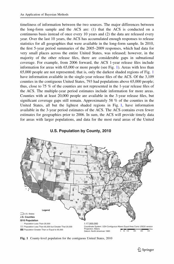
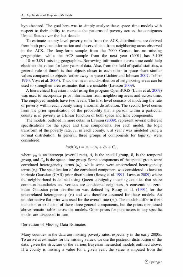
information for areas with 65,000 or more people (see Fig. 1). Areas with less than

65,000 people are not represented; that is, only the darkest shaded regions of Fig. 1

have information available in the single-year release files of the ACS. Of the 3,109

counties in the contiguous United States, 793 had populations above 65,000 people;

thus, close to 75 % of the counties are not represented in the 1-year release files of

the ACS. The multiple-year period estimates include information for more areas.

Counties with at least 20,000 people are available in the 3-year release files, but

significant coverage gaps still remain. Approximately 58 % of the counties in the

United States, all but the lightest shaded regions in Fig. 1, have information

available in the 3-year period estimates of the ACS. The ACS contains even fewer

estimates for geographies prior to 2006. In sum, the ACS will provide timely data

for areas with larger populations, and data for the most rural areas of the United

0 130 260 390 52065Miles

Legend

U.S. States

U.S. Counties

2010 PopulationPopulation Less Than 20,000

Population Less Than 65,000 but Greater That 20,000

Population Greater Than or Equal to 65,000

U.S. Population by County, 2010

Coordinate System: USA Contiguous Albers Equal Area Conic USGS versionProjection: AlbersDatum: North American 1983

1:17,000,000

Fig. 1 County-level population for the contiguous United States, 2010

An Application of Bayesian Methods

123

States will be available once enough responses are accumulated and averaged over

time. As a result, researchers now have the advantage of working with yearly

estimates for many sociodemographic measures; however, unless they are

comfortable working with period estimates, researchers interested in subnational

demographic processes are left to work with reduced sample sizes and a loss of data.

The goal of this research is to overcome the shortcomings of the ACS estimates

in order to take advantage of its benefits and create poverty estimates for every

county in the contiguous United States that does not have county-year ACS data. A

substantial amount of work has been done in the field of small area estimation (Rao

2003), and within this field, Bayesian approaches to small area estimation perhaps

give the most promise to providing stable and reliable estimates for missing

geographies in the ACS. Using a spatiotemporal smoothing process based upon

Bayesian statistics, information from neighboring areas as well as information

across time can be borrowed in order to generate reasonable estimates of rates in

counties not represented in the ACS. More specifically, four theoretical spatiotem-

poral models were examined in their ability to fit the ACS data, as well as their

ability to provide reliable estimates of county poverty rates for the contiguous

United States, and in their ability to recreate the spatial distribution of poverty in the

United States reported from extant sources. The primary advantage of these models

in terms of estimating poverty for small areas is their parsimonious specification.

That is, the models include terms for spatial information and temporal information

only. The rest of this report outlines the four different models and evaluates their

ability to recreate the known spatial and temporal distribution of poverty at the

county level for the contiguous United States.

Data

The ACS provides estimates counts of populations with certain characteristics

within US counties for each year since 2000. Estimates for persons below the

poverty threshold as well as estimated total counts of persons living within each of

the 3,109 counties in the contiguous United States over the 2000s were used for this

analysis. Estimates for 2001–2006 were obtained from the ACS 1-year sample.

Estimates for later periods were obtained from the multiple-year release files from

the ACS. How the multi-year estimates are actually used is discussed below. The

goal of this research is to investigate whether or not parsimonious models based on

publically available data can produce stable and reliable estimates of county-level

poverty rates that accurately depict the spatial and temporal pattern of US poverty

even with a minimal amount of data. The inclusion of the multiple-year data as

estimates for 2007–2010 is to investigate how the Bayesian models may be used

under varying degrees of missing data in an imputation fashion, where known data

are used to estimate unknown or missing observations. For simplicity, estimates are

referred to by the year of their release. For example, the 2008 3-year estimates are

actually obtained from the 2006–2008 ACS 3-year estimates, and the 2005–2009

ACS 5-year estimates are referred to as the 2009 5-year estimates. All of these

samples are grounded in the long-form data from Summary File 3 of the 2000

C. Sparks, J. Campbell

123

Census, and each is publicly available from the Census website (http://factfinder2.

census.gov/).

Incorporating multi-year ACS data is not a clear and unproblematic suggestion

(Citro and Kalton 2007; US Census Bureau 2008). To incorporate the three types of

estimates from the single-and multi-year data releases, we construct three separate

data sets, one for the single year, one for the 3-year and one for the 5-year estimate

releases. In each one of these data sets, a county is assigned the estimate for each

year it is represented in a particular data release. For example, Autauga County,

Alabama, had a population of 43,671 in 2000, but only 4,738 individuals with an

income below the poverty level. Since the population of this county was smaller

than 65,000 persons, the county had no single-year ACS data for any year between

2000 and 2010. The county did have 3-year estimates released in 2007, 2008, 2009

and 2010. Likewise, the county also had 5-year estimates released in 2009 and

2010.1 Using Autauga County as an example, our data table for it would be that

presented in Table 1.

To combine the various estimates of the population living below the poverty line,

the estimates for each year from the various data releases are averaged across all

available data. So, for 2005, the population estimates for county residents below the

poverty line were (5,223 ? 5,103)/2 = 5,163, while the estimate in 2009 was

(4,763 ? 5,341 ? 6,465 ? 5,103 ? 5,263)/5 = 5,387 persons. Undoubtedly, other

methods can be employed for combining these estimates, and this one may be

overly naı̈ve, but in this fashion, all data available from all estimates can be used in

the analysis. This process was repeated for the denominator populations for each

county for the population with a measured poverty status.

Since the model estimates for 2001–2006 are produced from average yearly

estimates using ACS 1-year estimates, particular attention will be given to how the

estimates of the missing geographies in these years behave. The estimates for later

years include data from multiple-year release files and were purposefully chosen to

determine how increasing the number of observed data can affect the estimates from

the models. Smoothing these estimates may not give researchers interested in

subnational sociodemographic processes the desired results as interpretation of

these rates may become cumbersome.

Poverty rates were chosen for two reasons. First, the importance of targeting anti-

poverty programs cannot be undersold (Baker and Grosh 1994; Bedi et al. 2007;

Bigman and Fofack 2000; Cuong 2011; Elbers et al. 2007). Identifying local areas

that have comparably larger rates of poverty is an invaluable tool to policy makers

and programs wishing to maximize the impact of anti-poverty strategies. Second,

the US Census Bureau routinely estimates poverty rates at the county level through

Small Area Income and Poverty Estimates (SAIPE) (Bell et al. 2007a, b). With the

support of various federal agencies, the US Census Bureau created the SAIPE

program to provide a number of income and poverty estimates separate from those

available the most recent Census (in our case the long-form data from Summary File

3 of the 2000 decennial Census).

1 At the time this analysis was conducted, the 2011 5-year ACS estimates had not been released.

An Application of Bayesian Methods

123

Ta

ble

1E

xam

ple

of

com

bin

ing

AC

Ses

tim

ates

for

ind

ivid

ual

sw

ith

inco

mes

bel

ow

the

po

ver

tyle

vel

for

Au

tau

ga

Co

un

ty,

Ala

bam

a(2

00

0–

20

11

)

Yea

r2

00

02

00

12

00

22

00

32

00

42

00

52

00

62

00

72

00

82

00

92

01

02

01

1

Cen

sus

20

00

4,7

38

––

––

––

––

––

–

AC

S1

yea

r–

––

––

––

––

––

–

AC

S3

yea

r(2

00

7)

––

––

–5

,223

5,2

23

5,2

23

––

––

AC

S3

yea

r(2

00

8)

––

––

––

5,6

94

5,6

94

5,6

94

––

–

AC

S3

yea

r(2

00

9)

––

––

––

–4

,763

4,7

63

4,7

63

––

AC

S3

yea

r(2

01

0)

––

––

––

––

5,3

41

5,3

41

5,3

41

–

AC

S3

yea

r(2

01

1)

––

––

––

––

–6

,46

56

,465

6,4

65

AC

S5

yea

r(2

00

9)

––

––

–5

,103

5,1

03

5,1

03

5,1

03

5,1

03

––

AC

S5

yea

r(2

01

0)

––

––

––

5,2

63

5,2

63

5,2

63

5,2

63

5,2

63

–

Com

bin

edes

tim

ate

(av

erag

eo

fea

chco

lum

n)

4,7

38

––

––

5,1

63

5,3

21

5,2

09

5,2

33

5,3

87

5,6

90

6,4

65

C. Sparks, J. Campbell

123

Area governments and resident decision makers rely on these estimates to

administer a variety of federal programs as well as allocate federal funds throughout

their local jurisdictions. Thus, county poverty estimates from SAIPE provide a

tested standard to which estimates from our hierarchical Bayesian models can be

compared. In addition, the SAIPE estimates serve as a glimpse into the changing

nature of poverty since there is an estimate for each year since 1989. As our time

window overlaps with that of SAIPE’s, maps of estimated poverty rates from our

models can be compared to maps of SAIPE estimates to examine whether the spatial

distribution of poverty is consistent. Error rates will also be calculated by

systematically comparing the hierarchical Bayesian estimates to the SAIPE

estimates to help determine how our model estimates of county-level poverty

compare to more established estimation procedures.

One last point about SAIPEs estimation method compared to the method

proposed in this report. The model specification outlined in the section below is

considerably different from the models used to estimate the numbers of poor via

SAIPE. SAIPE uses an empirical Bayes estimation method centered on a linear

regression. The dependent variable is the single-year county-level observations from

the ACS, and the independent variables come from the 2000 decennial Census,

postcensal population estimates, and administrative records like the number of tax

return exemptions, and the number of SNAP benefits recipients (see http://www.

census.gov/did/www/saipe/methods/ for more detailed information). While infor-

mation from the decennial Census and postcensal population estimates are widely

available, for many researchers, tax information and benefit recipient information is

not easy to obtain. Moreover, predictions from standard maximum likelihood

regression models are combined with the direct estimates from the ACS using

empirical Bayes techniques. This technique weights the contribution of the

regression predictions and ACS estimates to produce a single county estimate which

is then controlled to state and national estimates.

The Bayesian hierarchical models, outlined in more detail below, are decidedly

less complex. Simple specifications of spatial effects along with specified temporal

effects will be examined in their ability to provide a promising alternative to the

traditional empirical Bayes approach.

Methodology

Bayesian Estimation

Bayesian statistical methods have been popularized due to their ability to address

many issues related to small sample sizes and unstable estimates (Assuncao et al.

2002; Assuncao et al. 2005; Mckinnon et al. 2010; Potter et al. 2010). Improvements

in computer technology and the development of efficient sampling algorithms have

made it possible to employ these methods to a variety of applied problems (Lawson

2009).

Bayesian methods combine data with additional information in order to create

stronger and more stable measures. Referred to as a prior, this additional

An Application of Bayesian Methods

123

information is combined with observed data to obtain a posterior distribution.

Estimates and inferences are made from this posterior distribution. Priors can be

informative or diffuse, and constructing a posterior distribution can be very difficult,

especially if the form of the likelihood function, prior distribution, and the marginal

distribution involves complex formulas or models. Integrating complex posteriors

can be virtually impossible; however, it is possible to simulate a posterior

distribution using Monte Carlo Markov chain (MCMC) sampling methods (Hoff

2009).

Samples from the posterior distribution can be obtained using several different

MCMC methods. This research employs Gibbs sampling, which is one of the most

common methods for Bayesian estimation (Casella and George 1992; Gelman et al.

2003; Mckinnon et al. 2010). When using a Gibbs sampler to simulate a posterior

distribution, starting values for all parameters are first assigned. Then, new samples

for each parameter are made from the full conditional; that is, each parameter is

sampled from the distribution of that parameter conditioned on everything else. This

makes use of the most recent values of each parameter in the model and continually

updates the parameters with new values as soon as it has been sampled. Eventually,

the Markov chain converges so that values of all parameters are determined.

Model for Poverty Rates

In examining poverty rates within each county, an estimated count of the number of

people in poverty within each county was used. Define this count as yit and note that

there are i = 3,109 counties in the contiguous United States for each of the

t = 12 years included in this study. A population within each small area denoted nit

from which poverty counts are observed was also assumed. We form rates for each

county in each year as rit = yit/nit for counties that have observed ACS populations

constructed using the method described above. A normal model for the rate data in

each county is used. A logit transform of the rates is done to ensure that all

predictions are bound on [0,1], which has been used by other authors studying US

poverty rates (Friedman and Lichter 1998; Voss et al. 2006). The transform is of the

form yit = logit (rit) = ln(rit/(1 - rit)). The model likelihood is given by

Lðyjl; r2Þ ¼ 1

rffiffiffiffiffiffi

2pp e�

12

y�lrð Þ

2

A linear predictor for the mean of the model was constructed so that both spatial and

nonspatial components are incorporated in the model specification.

The Spatiotemporal Models

Providing a parsimonious description of the relative risk variation in space and time

could be important in providing reasonable estimates for missing data. Four models

that have been extensively examined in disease mapping applications were applied

to small area estimation of poverty rates and were chosen because of their

treatments of both space and time. They were not proposed as the best models for

this purpose but offer a plausible set of models, and alternative models could be

C. Sparks, J. Campbell

123

hypothesized. The goal here was to simply analyze these space–time models with

respect to their ability to recreate the patterns of poverty across the contiguous

United States over the last decade.

To estimate county-level poverty rates from the ACS, distributions are derived

from both previous information and observed data from neighboring areas observed

in the ACS. The long-form sample from the 2000 Census has no missing

geographies, while the ACS sample from the next year (2001) has 3,109

- 18 = 3,091 missing geographies. Borrowing information across time could help

elucidate the values for later years of data. Also, from the field of spatial statistics, a

general rule of thumb is that objects closer to each other in space share similar

values compared to objects farther away in space (Lichter and Johnson 2007; Tobler

1970; Voss et al. 2006). Thus, the mean and distribution of neighboring areas can be

used to strengthen area estimates that are unstable (Lawson 2009).

A hierarchical Bayesian model using the program OpenBUGS (Lunn et al. 2009)

was used to incorporate prior information from neighboring areas and across time.

The employed models have two levels. The first level consists of modeling the rate

of poverty within each county using a normal distribution. The second level comes

from the prior specification of the probability that a person within a particular

county is in poverty as a linear function of both space and time components.

The models, outlined in more detail in Lawson (2009), represent several different

specifications for the space and time components. For each model, the logit

transform of the poverty rate, rit, in each county, i, at year t was modeled using a

normal distribution. In general, three groups of components for logit(rit) were

considered:

logitðritÞ ¼ l0 þ Ai þ Bt þ Cit;

where l0 is an intercept (overall rate), Ai is the spatial group, Bt is the temporal

group, and Cit is the space–time group. Some components of the spatial group were

correlated heterogeneity terms (ui), while some were uncorrelated heterogeneity

terms (vi). The specification of the correlated component was considered to have an

intrinsic Gaussian (CAR) prior distribution (Besag et al. 1991; Lawson 2009) where

the neighborhood is defined using Queen contiguity meaning counties that share

common boundaries and vertices are considered neighbors. A conventional zero-

mean Gaussian prior distribution was defined by Besag et al. (1991) for the

uncorrelated heterogeneity (vi) and was therefore assumed for these models. An

uninformative flat prior was used for the overall rate (l0). The models differ in their

inclusion or exclusion of these three general components, but the priors mentioned

above remain stable across the models. Other priors for parameters in any specific

model are discussed in turn.

Derivation of Missing Data Estimates

Many counties in the data are missing poverty rates, especially in the early 2000s.

To arrive at estimates for the missing values, we use the posterior distribution of the

data, given the structure of the various Bayesian hierarchal models outlined above.

If a county is missing a value for a given year, the value is imputed from the

An Application of Bayesian Methods

123

posterior predictive distribution for that county and year, given the available

information and the model estimates, or more formally:

p yPredij jy

� �

¼Z

p yPredij jh

� �

pðhjyÞ;

which states that the posterior distribution for a missing county’s rate conditional on

the observed data is the posterior of the predicted value conditional on the current

estimates of the model parameters and the prior distribution. Thus, the model is used

to impute the missing values. This is implemented by first burning in the Markov

chains for 200,000 iterations, then doing 1,000 MCMC samples for each missing

value from the two converged Markov chains.

Model Specifications

For example, Model 1 is a variant of the model from Bernardinelli et al. (1995),

where the probability of being in poverty was modeled as

logitðritÞ ¼ l0 þ vi þ ui þ bt;

where l0 is an intercept (overall rate), and vi is an area (county) unstructured

heterogeneity (UH) random effect with prior distribution

pðviÞ / Nð0; svÞWith a mean of 0 and a precision of sv, where sv = 1/variance in the tradition of

Bayesian analysis, ui is a spatially correlated heterogeneity (CH) random effect with

a conditionally autoregressive normal prior,

pðuiÞ / Nðudi; su=ndiÞ

with ndi being the number of Queen contiguous spatial neighbors for county i, and bt

is a linear term in time t. A vague normal prior (0, .001) is used for b. In this case,

the model specification for the general model form is Ai = vi ? ui, Bt = bt, and

Cit = 0.

Model 2 is exactly like Model 1, except where time was a fixed linear effect in

Model 1, it is now a random effect in Model 2. The logit specification is of the form

logitðritÞ ¼ l0 þ vi þ ui þ tt;

where tt is a separate temporal random effect, with prior distribution tt * N(0, st),

and all other parameters are as they were in Model 1. In this formulation,

Ai = vi ? ui, Bt = tt, and Cit = 0.

Model 3 adds a temporally autoregressive heterogeneity term to Model 2 so that

the logit specification has the form

logitðritÞ ¼ l0 þ vi þ ui þ tt;

where l0 is an intercept (overall rate), vi is an area (county) random effect, ui is a

spatially correlated heterogeneity random effect, tt is a separate temporal random

effect with a first-order autoregressive prior distribution being used for tt: tt-

1 * N(tt-1, st). In this case, Ai = vi ? ui, Bt = tt and Cij = 0.

C. Sparks, J. Campbell

123

Model 4 was adopted from Knorr-Held (2000) who fit a space–time model using

88 counties in Ohio of lung cancer mortality data. This model includes a random

space–time interaction term. Here, the logit specification was defined in terms of

only random effects:

logitðritÞ ¼ l0 þ vi þ ui þ tt þ wit;

where the correlated and uncorrelated spatial components (ui, vi) are constant in

time. A separate temporal random effect (tt) and a space–time interaction term (wit)

were also included. In this formulation, Ai = vi ? ui, Bt = tt, and Cij = wit. Again,

an unstructured normal prior was used for tt, and the prior distribution for the

interaction term was simply a zero-mean normal. In the original source, this is

referred to as a Type I interaction model (Knorr-Held 2000) and is defined by the

prior distribution

pðwijÞ / Nð0; swÞ:

Diffuse inverse Gamma distributions (a = .5, 1/b = .0005) were assumed for all

hyperpriors in the models; that is, the precision parameters for the random effects

had diffuse inverse gamma distributions which penalize zero values but yield

considerable uniformity over a wide range (Lawson 2009). Precisions (1/variance)

are specified instead of variances following the tradition in Bayesian analysis.

Evaluation of Model Estimates

The traditional Bayesian method for model comparison is the Deviance Information

Criterion (DIC) (Spiegelhalter et al. 2002). However, this analysis focuses on

estimating missing data, and DIC as proposed by Spiegelhalter et al. (2002) is not

suitable for evaluating the complexity and fit of missing data models (Celeux et al.

2006). We attempt to calculate the DIC using the method discussed by Gelman and

colleagues (Gelman et al. 2003) who suggest using half the variance of the posterior

model deviance as a measure of the effective number of parameters. (Alonso-Villar

and Del Rio 2008)This estimates the DIC as:

DIC ¼ �Dþ cvarðDÞ;

with the general rule for model selection being that a smaller DIC indicates a better

fitting model.

While the method of using the model DIC as an indicator of relative model fit is

discussed widely, we take a conservative point of view, considering the discussion

of Celeux et al. (2006), and also consider other methods for examining model

estimates. These take the form of empirical comparisons of the Bayesian models to

the estimates produced by SAIPE for each time period. Mean Absolute Percent

Errors or similar comparisons commonly used in demography (Tayman and

Swanson 1999; Tayman et al. 1999) are one method of evaluating the closeness of

the Bayesian and SAIPE estimates, but they assume that the SAIPE estimates are

correct, when in fact both are estimates and there is no known ‘‘truth.’’ Instead of

making this assumption, several empirical comparisons of the Bayesian estimates

and the SAIPE estimates are conducted to judge the closeness of the estimates, with

An Application of Bayesian Methods

123

the logic being, if both sets of estimates tend to agree on a poverty rate for a given

county, then the estimates produced here are at least as good as those of the SAIPE.

The posterior mean poverty rate will be reported as the chosen estimate from our

proposed method, recognizing full well that the posterior median could be just as

suitable summary of the four models proposed. Using the posterior mean poverty

rate, comparisons of rates in counties across time, comparison of variances in the

national poverty rate across time, and maps of the differences between the

hierarchical Bayesian and SAIPE estimates to visualize where the two methods

diverge with respect to geography will be used to evaluate the closeness of our

estimates to those produced by SAIPE. t-tests for the mean difference between the

two estimates and F-ratio tests to examine differences in the variances between the

two sets of estimates will also be used. These are done on an annual basis for each

year in the data.

Results

Model Parameter Summaries

Table 2 provides the Bayesian point estimates, 95 % Bayesian credible intervals

(BCI) and model fit statistics for each of the four models described above. The CH

and UH parameters are quite stable across the four models. We also see that the

spatially correlated heterogeneity component of the model accounts for the most

variance in each model, generally being between 70 and 80 % of the total variance,2

except for Model 4, which has a high space–time variance component, and the CH

effects are only 28 % of the variance. There is a significant, but small temporal

Table 2 Posterior summaries of model parameters from the four Bayesian model specifications

Parameter Model 1 Model 2 Model 3 Model 4

Posterior mean

estimate

(95 % BCI)

Posterior mean

estimate

(95 % BCI)

Posterior mean

estimate

(95 % BCI)

Posterior mean

estimate

(95 % BCI)

Spatial UH (su) 990.1 (879.9,

1,115.0)

995.1 (884.9,

1119.0)

993.4 (882.6,

1,118.0)

991.9 (877.5,

1,117.0)

Spatial CH (sv) 218.9 (192.8,

248.5)

216.8 (191.1,

245.1)

217.2 (191.8,

246.8)

217.4 (192.0,

248.3)

Time trend (sb) 0.001 (0.002,

0.002)

– – –

Time random (st) – 1,143.5 (437.4,

2,179.0)

1,196.4 (441.6,

2320.0)

1,108.5 (413.6,

2154.0)

Space–time

random (sw)

– – – 99.1 (0.09, 496.1)

Deviance -135,700 -136,500 -136,308 -136,310

DIC -127,577 -128,328 -128,269 -128,374

2 The rule being applied here is r2 = 1/s, and % Spatial Variance = r2v=ðr2

v þ r2uÞ

C. Sparks, J. Campbell

123

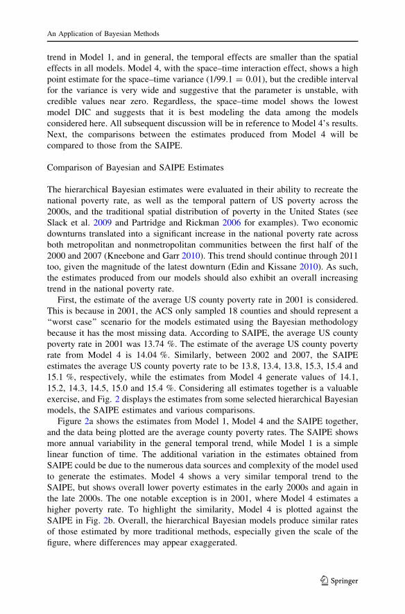
trend in Model 1, and in general, the temporal effects are smaller than the spatial

effects in all models. Model 4, with the space–time interaction effect, shows a high

point estimate for the space–time variance (1/99.1 = 0.01), but the credible interval

for the variance is very wide and suggestive that the parameter is unstable, with

credible values near zero. Regardless, the space–time model shows the lowest

model DIC and suggests that it is best modeling the data among the models

considered here. All subsequent discussion will be in reference to Model 4’s results.

Next, the comparisons between the estimates produced from Model 4 will be

compared to those from the SAIPE.

Comparison of Bayesian and SAIPE Estimates

The hierarchical Bayesian estimates were evaluated in their ability to recreate the

national poverty rate, as well as the temporal pattern of US poverty across the

2000s, and the traditional spatial distribution of poverty in the United States (see

Slack et al. 2009 and Partridge and Rickman 2006 for examples). Two economic

downturns translated into a significant increase in the national poverty rate across

both metropolitan and nonmetropolitan communities between the first half of the

2000 and 2007 (Kneebone and Garr 2010). This trend should continue through 2011

too, given the magnitude of the latest downturn (Edin and Kissane 2010). As such,

the estimates produced from our models should also exhibit an overall increasing

trend in the national poverty rate.

First, the estimate of the average US county poverty rate in 2001 is considered.

This is because in 2001, the ACS only sampled 18 counties and should represent a

‘‘worst case’’ scenario for the models estimated using the Bayesian methodology

because it has the most missing data. According to SAIPE, the average US county

poverty rate in 2001 was 13.74 %. The estimate of the average US county poverty

rate from Model 4 is 14.04 %. Similarly, between 2002 and 2007, the SAIPE

estimates the average US county poverty rate to be 13.8, 13.4, 13.8, 15.3, 15.4 and

15.1 %, respectively, while the estimates from Model 4 generate values of 14.1,

15.2, 14.3, 14.5, 15.0 and 15.4 %. Considering all estimates together is a valuable

exercise, and Fig. 2 displays the estimates from some selected hierarchical Bayesian

models, the SAIPE estimates and various comparisons.

Figure 2a shows the estimates from Model 1, Model 4 and the SAIPE together,

and the data being plotted are the average county poverty rates. The SAIPE shows

more annual variability in the general temporal trend, while Model 1 is a simple

linear function of time. The additional variation in the estimates obtained from

SAIPE could be due to the numerous data sources and complexity of the model used

to generate the estimates. Model 4 shows a very similar temporal trend to the

SAIPE, but shows overall lower poverty estimates in the early 2000s and again in

the late 2000s. The one notable exception is in 2001, where Model 4 estimates a

higher poverty rate. To highlight the similarity, Model 4 is plotted against the

SAIPE in Fig. 2b. Overall, the hierarchical Bayesian models produce similar rates

of those estimated by more traditional methods, especially given the scale of the

figure, where differences may appear exaggerated.

An Application of Bayesian Methods

123

To further examine the differences between the SAIPE and the Bayesian

estimates, means and variance tests are used. Figure 2c shows the raw difference

between the mean county poverty rate from SAIPE and from the Bayesian models,

alongside each annual difference is presented the probability of seeing such a

difference by random chance from a t distribution. The SAIPE and the Bayesian

models produce indistinguishable average county rates in 2000 and 2005–2006,

while the SAIPE produces lower estimates in the early 2000s and again in 2007 and

2008 and higher estimates from 2009 to 2011. There is a noticeable overall

increasing trend from 2000 to 2009 mirroring the expected trend in poverty. Despite

the illusion of statistical significance, the practical significance of these differences

is negligible, as enumerated in the text above. Indeed, the average difference

between the means across the whole period is -0.11 %, or on average the

hierarchical Bayesian models were .11 % higher than the SAIPE across this period.

When the variance in the estimates for the average US county poverty rate is

considered in Fig. 2d, the results show that the SAIPE had significantly lower levels

of county-to-county variation than the Bayesian models, especially in the early

2000s. This makes sense from two different perspectives. First, the early 2000s had

Fig. 2 Model estimates from the Bayesian models and comparisons to the SAIPE estimates

C. Sparks, J. Campbell

123

the least amount of data available to the hierarchical Bayesian models, so more

differences across counties are likely because of a lower degree of model specificity,

and the county estimates from the Bayesian models in these years are drawing

heavily from the 2000 estimate and the 2006 estimate for all strength. Secondly, the

Bayesian models have a spatially correlated smoothing term built into them, which

should serve to reduce the county-to-county variance, while preserving the mean.

The estimates obtained from this research suggest a clearer picture of subnational

poverty rates as they form a more cohesive picture of both county level and overall

poverty in the United States. While the overall temporal trend in the estimates

shows remarkable similarity, a second purpose of this paper is to recover the

geographic nature of poverty in US counties.

Geographic Distribution of Poverty

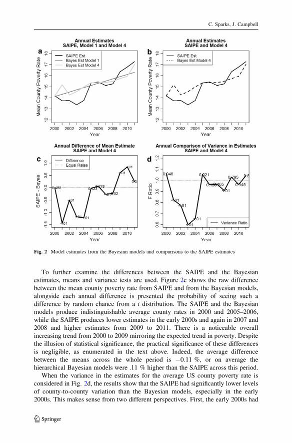
Figure 3 displays the posterior mean of the county poverty rate for each year from

Model 4. The patterning of poverty identified by the model mimics the spatial

patterning of poverty identified in the extant poverty literature (Lichter and Johnson

2007). That is, areas that are known to have high concentrations of impoverished

Fig. 3 Annual US county poverty rates derived from Model 4

An Application of Bayesian Methods

123

residents are also identified as high poverty areas with the hierarchical Bayesian

estimates. Extremely poor counties, distinguished by the darkest shade in the maps,

depict the same areas known to have heavy concentrations of poor residents.

Namely, Appalachia, which has been identified as a persistently poor area of the

United States (Cushing 1999; Pollard 2004), and the Native American reservations

on the Great Plains are both captured as high poverty areas in the maps of the

hierarchical Bayesian estimates. Poverty rates are often in excess of 50 % in

communities on the Pine Ridge Indian Reservation in South Dakota (O’Hare and

Johnson 2004) and are also in excess of 50 % in the hierarchical Bayesian model

estimates. Poverty rates are also known to be exceptionally high among African

Americans in the Mississippi Delta and ‘‘Black Belt’’ crescent (Lee and Singelmann

2005; Parisi et al. 2005), and among Mexican-origin Hispanics in the colonias of the

lower Rio Grande Valley (Saenz 1997; Saenz and Thomas 1991). Both of these

areas are identified in the maps of the hierarchical Bayesian estimates as having

particularly high poverty rates compared to other counties in the United States. In

sum, the noted patterns of poverty that exist in the United States are adequately

captured in all of the hierarchical Bayesian estimates.

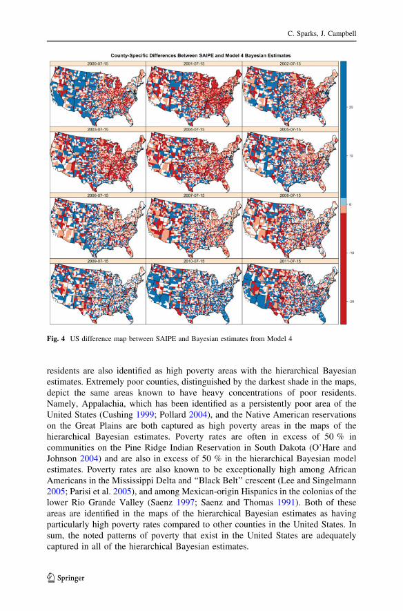
Fig. 4 US difference map between SAIPE and Bayesian estimates from Model 4

C. Sparks, J. Campbell

123

Figure 4 is perhaps the more interesting set of maps, where the quantity being

map is the difference between the posterior mean estimate from the fourth

hierarchical Bayesian model from Fig. 3 and the SAIPE point estimates.

The categories of differences in Fig. 4 were constructed based on the quartiles of

the difference distribution, with the lightest regions representing areas where the

map hierarchical Bayesian model was higher, and the darkest gray-shaded regions

representing areas where the SAIPE estimates had higher values. In the early 2000s,

the Bayesian model had higher estimates than the SAIPE in many areas of the

country, which corresponds to Fig. 2b, where the model was overall estimating a

higher poverty rate. After 2005, the differences between the two methods begin to

become less geographically clustered, and then again, in 2010 and 2011, the

differences again show notable geographic clusters in the southeast, with the SAIPE

having higher values. Again, this mirrors the differences seen in Fig. 2b.

A final comparison is made between the SAIPE and the Bayesian estimates. For

this comparison, the quartiles of the estimates for all years are used. For each year,

both types of estimates are classified by the quartile their particular values fall into.

If the two values from the two methods of estimation for a particular county agree,

then their estimates for each year should at least be in the same quartile as one

another. This is a form of classification comparison, and the percent of counties

sharing a common classification should tell how close the estimates are to one

another. This gives another clue to the closeness of the estimates produced by the

two different methodologies, without worrying about the exactness of the two

estimates. Figure 5 presents a graphical summary of this comparison, with the

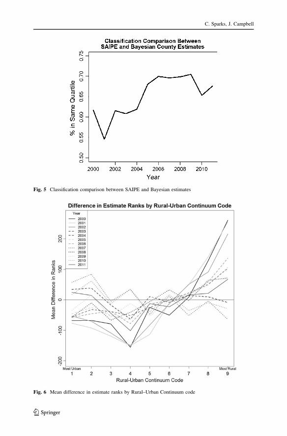
percent of counties sharing a common classification on the y axis.

On average, 65 % of counties across the 12-year period under consideration

shared the same quartile between the two types of estimate. The range was between

54 % in 2001 (the year with the least data) and 70 % in 2009 (the year with the most

data). This suggests that both types of estimates are close to each other in the

majority of counties.

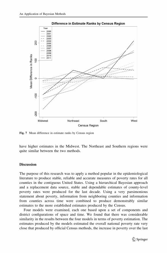
To further summarize the geographic patterns of the rate estimates, the estimates

from the SAIPE and the Bayesian methods were ranked from highest to lowest for

each year. The differences between the ranks were then formed and summarized by

type of county, as measured by the USDA’s Rural–Urban Continuum code

classifications and by Census region. These results are presented, respectively, in

Figs. 6 and 7 below.

Figure 6 shows the mean difference in a county’s ranks from the two forms of

estimation. For example, Bexar County, TX, was ranked 2,178th (out of 3,109) in

the nation in 2001 according to the SAIPE, and the method used here, the county

was ranked 2,053rd, a difference in ranks of 125. For this comparison, a positive

difference means that the SAIPE estimate was higher than our estimate and vice

versa. Graphically, the SAIPE estimates were on average higher in the most rural

counties (counties not adjacent to a metro area, of a completely rural nature and less

than 2,500 persons), while the estimates derived here were higher in areas that were

nonmetro, but adjacent to a metro county with 20,000 persons or more.

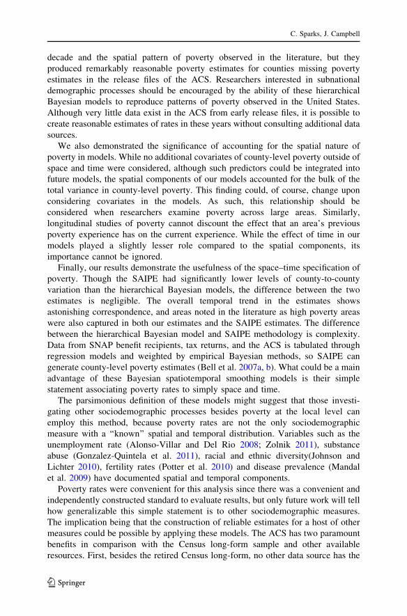
Further illustration in Fig. 7 shows that on average, the SAIPE had higher

poverty estimates in the Western region than the current method, while we tended to

An Application of Bayesian Methods

123

Fig. 5 Classification comparison between SAIPE and Bayesian estimates

Fig. 6 Mean difference in estimate ranks by Rural–Urban Continuum code

C. Sparks, J. Campbell

123

have higher estimates in the Midwest. The Northeast and Southern regions were

quite similar between the two methods.

Discussion

The purpose of this research was to apply a method popular in the epidemiological

literature to produce stable, reliable and accurate measures of poverty rates for all

counties in the contiguous United States. Using a hierarchical Bayesian approach

and a replacement data source, stable and dependable estimates of county-level

poverty rates were produced for the last decade. Using a very parsimonious

statement about poverty, information from neighboring counties and information

from counties across time were combined to produce demonstrably similar

estimates to the more established estimates produced by the Census.

Four models were examined, each one based upon a set of components and

district configurations of space and time. We found that there was considerable

similarity in the results between the four models in terms of poverty estimation. The

estimates produced by the models estimated the overall national poverty rate very

close that produced by official Census methods, the increase in poverty over the last

Fig. 7 Mean difference in estimate ranks by Census region

An Application of Bayesian Methods

123

decade and the spatial pattern of poverty observed in the literature, but they

produced remarkably reasonable poverty estimates for counties missing poverty

estimates in the release files of the ACS. Researchers interested in subnational

demographic processes should be encouraged by the ability of these hierarchical

Bayesian models to reproduce patterns of poverty observed in the United States.

Although very little data exist in the ACS from early release files, it is possible to

create reasonable estimates of rates in these years without consulting additional data

sources.

We also demonstrated the significance of accounting for the spatial nature of

poverty in models. While no additional covariates of county-level poverty outside of

space and time were considered, although such predictors could be integrated into

future models, the spatial components of our models accounted for the bulk of the

total variance in county-level poverty. This finding could, of course, change upon

considering covariates in the models. As such, this relationship should be

considered when researchers examine poverty across large areas. Similarly,

longitudinal studies of poverty cannot discount the effect that an area’s previous

poverty experience has on the current experience. While the effect of time in our

models played a slightly lesser role compared to the spatial components, its

importance cannot be ignored.

Finally, our results demonstrate the usefulness of the space–time specification of

poverty. Though the SAIPE had significantly lower levels of county-to-county

variation than the hierarchical Bayesian models, the difference between the two

estimates is negligible. The overall temporal trend in the estimates shows

astonishing correspondence, and areas noted in the literature as high poverty areas

were also captured in both our estimates and the SAIPE estimates. The difference

between the hierarchical Bayesian model and SAIPE methodology is complexity.

Data from SNAP benefit recipients, tax returns, and the ACS is tabulated through

regression models and weighted by empirical Bayesian methods, so SAIPE can

generate county-level poverty estimates (Bell et al. 2007a, b). What could be a main

advantage of these Bayesian spatiotemporal smoothing models is their simple

statement associating poverty rates to simply space and time.

The parsimonious definition of these models might suggest that those investi-

gating other sociodemographic processes besides poverty at the local level can

employ this method, because poverty rates are not the only sociodemographic

measure with a ‘‘known’’ spatial and temporal distribution. Variables such as the

unemployment rate (Alonso-Villar and Del Rio 2008; Zolnik 2011), substance

abuse (Gonzalez-Quintela et al. 2011), racial and ethnic diversity(Johnson and

Lichter 2010), fertility rates (Potter et al. 2010) and disease prevalence (Mandal

et al. 2009) have documented spatial and temporal components.

Poverty rates were convenient for this analysis since there was a convenient and

independently constructed standard to evaluate results, but only future work will tell

how generalizable this simple statement is to other sociodemographic measures.

The implication being that the construction of reliable estimates for a host of other

measures could be possible by applying these models. The ACS has two paramount

benefits in comparison with the Census long-form sample and other available

resources. First, besides the retired Census long-form, no other data source has the

C. Sparks, J. Campbell

123

amount of detailed information at the county level than the ACS. Secondly, the

frequency that ACS estimates are produced provides a welcome alternative to often

aging estimates when examining social and economic outcomes. Policy makers and

researchers alike relied heavily on the decennial Census products to help analyze

trends and make decisions. As a decade wears on, however, the information in the

decennial Census gets less relevant. The frequency with which ACS data products

are produced ensures that policy makers will have more current information well

into the decade between Censuses.

Researchers used to working with Census long-form data must now rely on ACS

data products to help answer their research questions, and this analysis demonstrates

that accurate and reasonable estimates of missing values can be obtained with

relative ease. Currently, there are overlapping multiple-year summary files of the

ACS, but in the not-so-distant future, the ACS will have amassed multi-year files

that will not overlap. That means wider coverage geographically and an added

element of precision for policy makers looking to target policies to areas in need.

Acknowledgments We gratefully acknowledge the advice of the four anonymous reviewers, whose

comments greatly improved the quality of this manuscript. This paper was originally presented at the

Population Association of America annual meeting in San Francisco, CA.

References

Alonso-Villar, O., & Del Rio, C. (2008). Geographical concentration of unemployment: A male-female

comparison in Spain. Regional Studies, 42(3), 401–412. doi:10.1080/00343400701291559.

Assuncao, R. M., Potter, J. E., & Cavenaghi, S. M. (2002). A Bayesian space varying parameter model

applied to estimating fertility schedules. Statistics in Medicine, 21(14), 2057–2075. doi:10.1002/sim.

1153.

Assuncao, R. M., Schmertmann, C. P., Potter, J. E., & Cavenaghi, S. M. (2005). Empirical Bayes

estimation of demographic schedules for small areas. Demography, 42(3), 537–558. doi:10.1353/

dem.2005.0022.

Baker, J. L., & Grosh, M. E. (1994). Poverty reduction through geographic targeting—How well does it

work? World Development, 22(7), 983–995. doi:10.1016/0305-750x(94)90143-0.

Bedi, T., Coudouel, A., & Simler, K. (2007). More than a pretty picture: Using poverty maps to design

better policies and interventions Poverty Reduction & Equity. Washington, DC: The World Bank.

Bell, W., Basel, W., Cruse, C., Dalzell, L., Maples, J., O’Hara, B., et al. (2007). In U. S. C. Bureau (Ed.).

Use of ACS data to produce SAIPE model-based estimates of poverty for counties. Washington,

DC: U.S. Census Bureau.

Bell, W., Basel, W., Cruse, C., Dalzell, L., Maples, J., O’Hara, B., et al. (2007). Use of ACS data to

produce SAIPE model-based estimates of poverty for counties. Washington, DC: U.S. Census

Bureau. Retrieved from http://www.census.gov/did/www/saipe/publications/files/report.pdf.

Bernardinelli, L., Clayton, D., Pascutto, C., Montomoli, C., Ghislandi, M., & Songini, M. (1995). Bayesian

analysis of space–time variation in disease risk. [Article]. Statistics in Medicine, 14(21–22), 2433–2443.

doi:10.1002/sim.4780142112.

Besag, J., York, J. C., & Mollie, A. (1991). Bayesian Image Restoration, with two applications in

spatial statistics (with discussion). Annals of the Institute of Statistical Mathematics, 43(1), 1–59.

doi:10.1007/BF00116466.

Bigman, D., & Fofack, H. (2000). Geographical targeting for poverty alleviation: Methodology and

applications Regional and Sectoral Studies (Vol. 1). Washington, DC: The World Bank.

Casella, G., & George, E. I. (1992). Explaining the Gibbs sampler. The American Statistician, 46(3),

167–174.

An Application of Bayesian Methods

123

Celeux, G., Forbes, F., Robert, C. P., & Titterington, D. M. (2006). Deviance information criteria for

missing data models. Bayesian Analysis, 1(4), 651–673.

Census Bureau, U. S. (2008). A compass for understanding and using American Community Survey data:

What general data users need to know. Washington, DC: U.S. Government Printing Office.

Citro, C. E., & Kalton, G. (Eds.). (2007). Using the American community survey: Benefits and challenges.

Washington, DC: The National Academy Press.

Cuong, N. V. (2011). Poverty projection using a small area estimation method: Evidence from Vietnam.

Journal of Comparative Economics, 39(3), 368–382. doi:10.1016/j.jce.2011.04.004.

Cushing, B. (1999). In K. Pandit & S. D. Withers (Eds.), Migration and persistent poverty in rural

America. Lanham, MD: Rowmen and Littlefield press.

Edin, K., & Kissane, R. J. (2010). Poverty and the American family: A decade in review. Journal of

Marriage and Family, 72(3), 460–479. doi:10.1111/j.1741-3737.2010.00713.x.

Elbers, C., Fujii, T., Lanjouw, P., Ozler, B., & Yin, W. (2007). Poverty alleviation through geographic

targeting: How much does disaggregation help? Journal of Development Economics, 83(1),

198–213. doi:10.1016/j.jdeveco.2006.02.001.

Friedman, S., & Lichter, D. T. (1998). Spatial inequality and poverty among American children.

Population Research and Policy Review, 17(2), 91–109. doi:10.1023/A:1005740205017.

Gelman, A. E., Carlin, J. B., Stern, H. S., & Rubin, D. B. (2003). Bayesian data analysis, 2nd Edn (2nd

ed.). Boca Raton, FL: Chapman & Hall/CRC.

Gonzalez-Quintela, A., Fernandez-Conde, S., Alves, M. T., Campos, J., Lopez-Raton, M., Puerta, R.,

et al. (2011). Temporal and spatial patterns in the rate of alcohol withdrawal syndrome in a defined

community. Alcohol, 45(2), 105–111. doi:10.1016/j.alcohol.2010.08.001.

Hoff, P. D. (2009). A first course in Bayesian statistical methods. Boca Raton, FL: Chapman & Hall/CRC.

Johnson, K. M., & Lichter, D. T. (2010). Growing diversity among America’s children and youth: Spatial

and temporal dimensions. Population and Development Review, 36(1), 151?.

Kneebone, E., & Garr, E. (2010). The suburbanization of poverty: Trends in metropolitan America, 2000

to 2008 Metropolitan opportunity series. Washington, DC: The Brookings Institution.

Knorr-Held, L. (2000). Bayesian modelling of inseparable space–time variation in disease risk. Statistics

in Medicine, 19(17–18), 2555–2567. doi:10.1002/1097-0258(20000915/30)19:17/18\2555::AID-

SIM587[3.0.CO;2-#.

Lawson, A. B. (2009). Bayesian disease mapping. Boca Raton, FL: Chapman & Hall/CRC.

Lee, M. A., & Singelmann, J. (2005). Welfare reform amidst chronic poverty in the Mississipi delta. In

W. A. Kandel & D. L. Brown (Eds.), Population change and rural society. Dordrecht: Springer.

Lichter, D. T., & Johnson, K. M. (2007). The changing spatial concentration of America’s rural poor

population. Rural Sociology, 72(3), 331–358. doi:10.1526/003601107781799290.

Lunn, D., Spiegelhalter, D., Thomas, A., & Best, N. (2009). The BUGS project: Evolution, critique and

future directions (with discussion). Statistics in Medicine, 28(25), 3049–3067. doi:10.1002/sim.

3680.

Mandal, R., St-Hilaire, S., Kie, J. G., & Derryberry, D. (2009). Spatial trends of breast and prostate

cancers in the United States between 2000 and 2005. International Journal of Health Geographics,

8, 53. doi:10.1186/1476-072x-8-53.

Mckinnon, S., Potter, J. E., & Schmertmann, C. S. (2010). Municipality-level estimates of child mortality

for Brazil: A new approach using Bayesian Statistics. Paper presented at the Population Association

of America 2010 Annual Meeting, Dallas, TX. http://paa2010.princeton.edu/download.aspx?

submissionId=101738.

O’Hare, W. P., & Johnson, K. M. (2004). Child poverty in rural America Reports on America (Vol. 4).

Washington, DC: Population Reference Bureau.

Parisi, D., Grice, S., Taquino, M., & Gill, D. (2005). Community concentration of poverty and its

consequences on nonmetro county persistence of poverty in Mississippi. Sociological Spectrum,

25(4), 469–483. doi:10.1080/027321790947234.

Partridge, M. D., & Rickman, D. S. (2006). The geography of American poverty: Is there a need for

place-based policies. Kalamazoo, MI: W. E. Upjohn Institute for Employment Research.

Pollard, K. M. (2004). A ‘New Diversity’: Race and ethnicity in the Appalachian Region. Demographic

and socioeconomic change in Appalachia. Washington, DC: Population Reference Bureau.

Potter, J. E., Schmertmann, C. P., Assuncao, R. M., & Cavenaghi, S. M. (2010). Mapping the timing,

pace, and scale of the fertility transition in Brazil. Population and Development Review, 36(2),

283–307. doi:10.1111/j.1728-4457.2010.00330.x.

Rao, J. K. (2003). Small Area Estimation. Hoboken, NJ): Wiley.

C. Sparks, J. Campbell

123

Saenz, R. (1997). Ethnic concentration and Chicano poverty: A comparative approach. Social Science

Research, 26(2), 205–228. doi:10.1006/ssre.1997.0595.

Saenz, R., & Thomas, J. K. (1991). Minority poverty in Nonmetropolitan Texas. Rural Sociology, 56(2),

204–223.

Slack, T. L., Singelmann, J., Fontenot, K., Poston, D., Seanz, R., & Siodia, C. (2009). Poverty in the

Texas borderland and lower Mississippi delta: A comparative analysis of differences by family type.

Demographic Research, 20, 353–376.

Spiegelhalter, D. J., Best, N. G., Carlin, B. R., & van der Linde, A. (2002). Bayesian measures of model

complexity and fit. Journal of the Royal Statistical Society Series B-Statistical Methodology, 64,

583–616. doi:10.1111/1467-9868.00353.

Tayman, J., & Swanson, D. A. (1999). On the validity of MAPE as a measure of population forecast

accuracy. Population Research and Policy Review, 18(4), 299–322. doi:10.1023/A:1006166418051.

Tayman, J., Swanson, D. A., & Barr, C. F. (1999). In search of the ideal measure of accuracy for

subnational demographic forecasts. Population Research and Policy Review, 18(5), 387–409.

Tobler, W. (1970). A computer movie simulating population growth in the Detroit region. Economic

Geography, 42, 234–240.

U.S. Department of Commerce, Bureau of the Census, U.S. Department of Labor, & Bureau of Labor

Statistics. (1976). Concepts and methods used in labor force statistics derived from the Current

Population Survey Current Population Reports. Washington, DC.

Voss, P., Long, D. D., Hammer, R. B., & Friedman, S. (2006). County child poverty rates in the U.S.: A

spatial regression approach. Population Research and Policy Review, 25(4), 369–391. doi:10.1007/

s11113-006-9007-4.

Zolnik, E. J. (2011). The geographic distribution of US unemployment by gender. Economic Development

Quarterly, 25(1), 91–103. doi:10.1177/0891242410386592.

An Application of Bayesian Methods

123