An application of indirect model reference adaptive controlto a low-power proton exchange membrane fuel cell
Yee-Pien Yang ∗, Zhao-Wei Liu, Fu-Cheng WangDepartment of Mechanical Engineering, National Taiwan University, Taipei, Taiwan, ROC
Received 5 December 2007; received in revised form 24 January 2008; accepted 24 January 2008Available online 6 February 2008
bstract
Nonlinearity and the time-varying dynamics of fuel cell systems make it complex to design a controller for improving output performance. Thisaper introduces an application of a model reference adaptive control to a low-power proton exchange membrane (PEM) fuel cell system, whichonsists of three main components: a fuel cell stack, an air pump to supply air, and a solenoid valve to adjust hydrogen flow. From the systemerspective, the dynamic model of the PEM fuel cell stack can be expressed as a multivariable configuration of two inputs, hydrogen and air-flowates, and two outputs, cell voltage and current. The corresponding transfer functions can be identified off-line to describe the linearized dynamicsith a finite order at a certain operating point, and are written in a discrete-time auto-regressive moving-average model for on-line estimation of
arameters. This provides a strategy of regulating the voltage and current of the fuel cell by adaptively adjusting the flow rates of air and hydrogen.xperiments show that the proposed adaptive controller is robust to the variation of fuel cell system dynamics and power request. Additionally, itelps decrease fuel consumption and relieves the DC/DC converter in regulating the fluctuating cell voltage.
2008 Elsevier B.V. All rights reserved.
eywords: PEM fuel cell; System identification; Model reference adaptive control
vv
ucpvclcnhca
. Introduction
Proton exchange membrane fuel cells, also known as poly-er electrolyte membrane fuel cells, have the advantages of
igh power and energy density, low operation temperature, fasttart-up, and higher efficiency, but still face many challengingechnical hurdles, such as cost, size, weight, durability, reliabil-ty, and air, thermal, and water management [1–3]. In addition,uel cells are subjected to various situations of time-varying load,uring which the air-flow, gas pressure, temperature, humid-ty, and membrane hydration must be controlled over a wideange of operation. Typical fuel cell system operation requiresrompt measurement of system states by a set of sensors, suchs flow meters, thermocouples, pressure transducers, voltmeter,
all sensor, hydrogen detector, etc. These signals are typicallyed back to a microprocessor that calculates proper controlctions based on a specific control strategy that is executed by
arious actuators, such as an air pump, a humidifier, solenoidalves, fan motors and safety devices.
The complex, nonlinear dynamics of fuel cell systems aresually approximately described by the principles of electro-hemistry, fluid dynamics, and heat transfer in terms of physicalarameters, material properties, and universal constants underarious assumptions and constraints. The dynamic response ofell voltage and current involve reactant pressure and flow rate,ocal species concentration, and load electrical demands, whichan vary rapidly enough that many assume these are instanta-eous. On the other hand, fuel cell temperature and its regulation,umidity, cell hydration, as well as overall heat management pro-esses are characterized by relatively slow dynamic response, asnalyzed by Mueller et al. [4]. Many researchers have devotedhemselves to developing and using steady-state models of PEMuel cells, describing the relationships amongst physical vari-bles through the Nernst equation, gas diffusion equation, and
pecies concentration and polarization equations. Most recently,n increasing number of researchers have focused on dynamicodels to describe the transient response of PEM fuel cell sys-
ems. Pukrushpan et al. [5] modeled transient dynamics with
awmcatJaadecofland ribs in an active area of 40 mm × 130 mm.
The rated and peak power outputs of the fuel cell are 117 Wat 9 V and 124 W at 7.9 V, respectively. The maximum fuel-to-electricity efficiency that the fuel cell can achieve is about
Y.-P. Yang et al. / Journal of P
set of first-order differential equations governing the air com-ressor, mass transportation, energy conservation of the reactantows, and pressures in the cathode and anode. Ceraolo et al. [6]rovided more precise partial differential equations to describeoth static and dynamic behaviors of the PEM fuel cell, includingas diffusion, proton concentration, and mass transportation. Inheir spatial, time-dependent fuel cell model, Golbert and Lewin7] included the dynamics of water condensation, evaporation,nd generation, as well as quasi-steady-state temperature profile.athapati et al. [8] derived a dynamic model with the effects ofharge double-layer capacitance, dynamics of flow and pressure,nd mass/heat transient features of fuel cells, which predicted theransient response of cell voltage, temperature, gas flow rates,nd pressure under a sudden change in load current. A highlyynamic PEM fuel cell stack model was proposed by Shan andhoe [9], which took into account the most influential propertyf temperature on the output performance and dynamics.
Although some researchers have proposed an effective modelor system and control development [4,10], the nonlinearitynd time-varying characteristics still pose difficult problemsor system identification and control. Simplified models, eitherinear or nonlinear, with nominal parameters are usually validithin a linear range of operation. Such models are usually used
o investigate stability, sensitivity, observability, and control-ability, before designing a controller. More practically, thesearameters that vary with time and operating states are identi-ed in real time to match system response with minimal errors.herefore, adaptive control can serve as a feedback law tochieve control objectives subject to the variation of systemarameters as well as external disturbances. Pukrushpan et al.5] designed an observer-based feedback controller to protecthe fuel cell stack from oxygen starvation during the change ofurrent command, using the linear quadratic technique based onhe linearized state-space model. Paradkar et al. [11] integrated ainearized PEM fuel cell model into a power plant, and simulatedload frequency control problem by an optimal controller basedn the disturbance accommodation control theory. Schumachert al. [12] employed a fuzzy controller to manage humidity bydjusting the fan voltage for supplying air to a miniature PEM.urado and Saenz [13] noted that their proposed adaptive controltrategy was able to stabilize a hybrid fuel cell and turbine systemubject to system parameter variations and external disturbances.ekin et al. [14] provided a fuzzy proportional-derivative (PD)ontroller plus integral (I) controller to adjust the air-flow ratef a 5 KW PEM fuel cell. It was found that the ratio betweenhe consumed energy by the motor-compressor group and thenergy delivered by the fuel cell was greatly reduced. Woo andenziger [15] applied a PID controller to regulate the output cur-
ent of a single-cell PEM fuel cell by controlling the flow ratef hydrogen, while the full utilization of hydrogen was achievedith 30% stoichiometric excess on the oxygen.Recently, Meyer and Revankar [16] surveyed the control-
riented models and control strategies of PEM fuel cell systems.
he researchers indicated that future attempts to develop nonlin-ar multi-input multi-output systems must be important over thentire operating range in order to seek reduced reactant usagender various power demands. Methekar et al. [17] proposed
Sources 179 (2008) 618–630 619
linear multivariable model for controlling the average powerensity and solid temperature of a PEM fuel cell to avoid oxygentarvation. The selected input variables were the inlet molar flowate of hydrogen, the inlet molar flow rate of oxygen, the inletow rate of coolant, and the inlet gas temperatures of anodes andathodes. These researchers simulated the order reduction fromdistributed parameter model to a set of first- or second-order
ransfer functions, by which the PI-controller-based power andolid temperature control loops were constructed.
The authors have also presented a preliminary study of systemdentification, and robust and adaptive controls of a low-powerEM fuel cell [18,19]. This paper extends the previous single-
nput single-output (SISO) adaptive control to a multivariableonfiguration of indirect model reference adaptive control. Bothhe air and hydrogen flow rates are used to regulate cell voltagend current according to the updated information of the externaload and system dynamics.
. Material and methods
.1. Fuel cell specifications
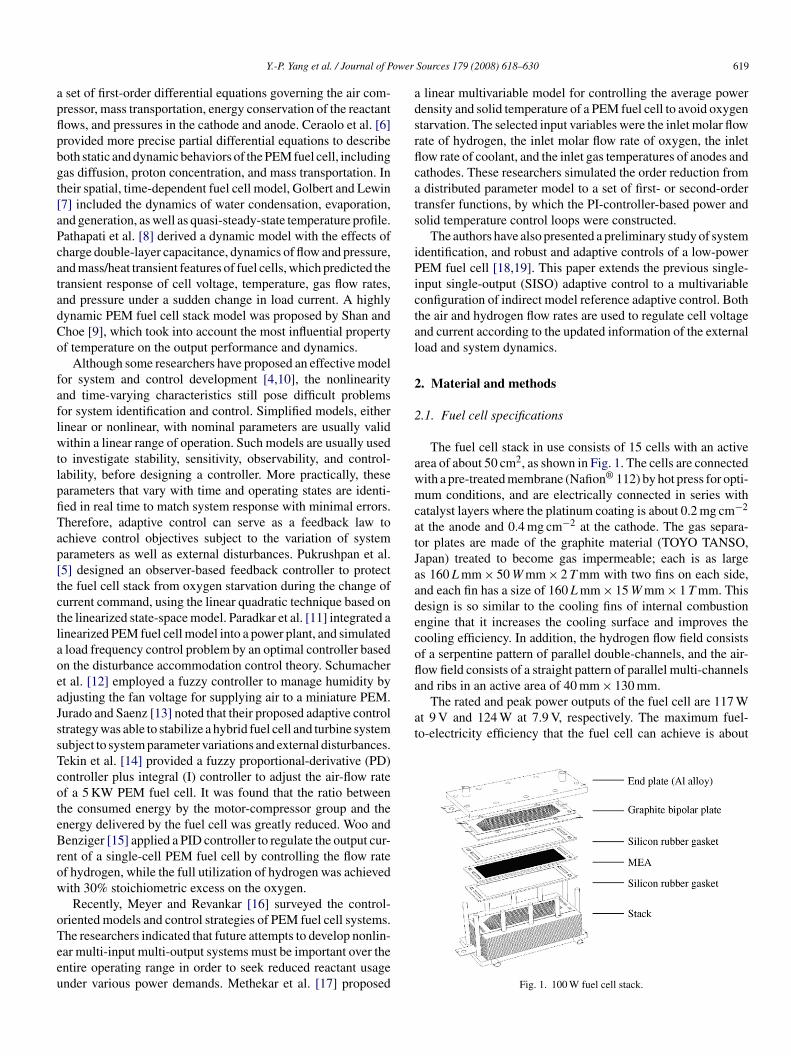
The fuel cell stack in use consists of 15 cells with an activerea of about 50 cm2, as shown in Fig. 1. The cells are connectedith a pre-treated membrane (Nafion® 112) by hot press for opti-um conditions, and are electrically connected in series with
atalyst layers where the platinum coating is about 0.2 mg cm−2
t the anode and 0.4 mg cm−2 at the cathode. The gas separa-or plates are made of the graphite material (TOYO TANSO,apan) treated to become gas impermeable; each is as larges 160 L mm × 50 W mm × 2 T mm with two fins on each side,nd each fin has a size of 160 L mm × 15 W mm × 1 T mm. Thisesign is so similar to the cooling fins of internal combustionngine that it increases the cooling surface and improves theooling efficiency. In addition, the hydrogen flow field consistsf a serpentine pattern of parallel double-channels, and the air-ow field consists of a straight pattern of parallel multi-channels
Fig. 1. 100 W fuel cell stack.
620 Y.-P. Yang et al. / Journal of Power Sources 179 (2008) 618–630
cell s
3htiacupv
2
ctecrbFpss
i
bflstbfliIflchtilcvpaWrI
Fig. 2. PEM fuel
7% on a lower heating value (LHV) under the dry H2/air andumidification-free conditions. The fuel cell system was a pro-otype from Delta Electronics. The whole system includes anndividual temperature control loop, water management loop,nd flow control loop. This paper intends to replace the flowontrol loop using adaptive control while keeping the othersnchanged. The flow rate of natural air is adjusted by an airump, while the flow rate of hydrogen is regulated by a solenoidalve.
.2. Fuel cell system model
In order to develop the control strategy of the low-power fuelell, the dynamic models from the previous studies are integratedo describe the mass and heat transfer in flow channels, Nernstquation, cathode gas diffusion, cathode kinetics, and protononcentration dynamics [6,20–23]. From modern control theo-ies [24], the control-oriented fuel cell system block diagram cane approximated as a two-input two-output system, as shown inig. 2. Equipped with additional balance-of-plant (BOP) com-onents, such as an air pump and hydrogen valve, the fuel cell
ystem can be simply reduced to a standard block diagram, ashown in Fig. 3.
From the system viewpoint, the hydrogen at a certain pressures fed by a solenoid valve whose dynamics are denoted by the
Fig. 3. Approximate fuel cell system block diagram.
b
V
I
wS
V
dpstc
ystem dynamics.
lock GS that describes the relationship between the hydrogenow rate NH and valve voltage VS. On the other hand, air at thetandard atmosphere of 1 bar is often transported by an air pumpo provide oxygen to the cathode, whose dynamics are denotedy the block Ga that describes the relationship between the air-ow rate NA and air pump voltage VA. The coupled blocks Gi,= 1, 2, 3, 4, describe the relationships between the cell currentc and cell voltage Vc, and the air-flow rate NA and hydrogenow rate NH, where R denotes the internal resistance of the fuelell. It is noticed that the temperature and humidity of air andydrogen are not managed in this research, but are regarded aswo dependent states of the fuel cell. Assuming that the fuel cells operated at a certain operating point, the six blocks can beinearized as transfer functions of finite orders and time-varyingoefficients. These coefficients are implicit functions of stateariables, such as temperature, membrane hydration, reactantressure, gas concentration, etc., which directly affect cell volt-ge, current density, and the overall performance of the fuel cell.hen the air pump voltage and the hydrogen valve voltage are
egarded as input variables, and the cell voltage Vc and currentc are chosen as system outputs, the fuel cell system model cane expressed as
c = Ga2VA + GS4VS − RIc, (1)
c = Ga1VA + GS3VS, (2)
here Ga1 = GaG1, Ga2 = GaG2, GS3 = GSG3, GS4 = GSG4.ince Vc and Ic are dependent, (1) can be reduced to
c = (Ga2 − RGa1)VA + (GS4 − RGa1)VS. (3)
It is noticed that the cell voltage and cell current, since depen-ent, are not to be regulated concurrently with arbitrary set
oints. Either configuration (2) or (3), namely a multi-inputingle-output model, is employed as the basis of system iden-ification, as well as an adjustable model for designing the fuelell controller.
Y.-P. Yang et al. / Journal of Power Sources 179 (2008) 618–630 621
Table 1Operating conditions for system identification
Temperature (◦C) 17Pressure (atm) 1Humidity (%) 74Fuel cell temperature (◦C) 35–40Air pump voltage (V) 5 ± 2Anode reactant H2, 1.2 LPM, 7 psigCathode reactant Natural airC −2
S
2
t(tdmcr
duhaoEuwhha
8aqaaG
|
φ
w
f
Fof
F
tstTo facilitate the following adaptive controller design, a setof second-order continuous-time transfer functions and theirdiscrete-time approximations of 0.01 s sampling time at a certainoperating point are illustrated in Table 2.
Table 2Illustration of identified second-order transfer function pairs in s and z domains
Ga1 = Ic/VA, Vc = 8 V Ga2 = Vc/VA, Ic = 3 A
0.9909s + 15.89
s2 + 6.401s + 9.732
0.3269s + 2.016
s2 + 3.921s + 2.058
0.01037z − 0.008835
z2 − 1.937z + 0.938
0.003305z − 0.003107
z2 − 1.961z + 0.9616
GS3 = Ic/VS, Vc = 8 V GS4 = Vc/VS, Ic = 3 A
0.2477s + 3.973 0.08173s + 0.5041
urrent density (A cm ) 0.2ampling frequency (Hz) 100
.3. Off-line system identification
The purpose of off-line system identification is to obtain theransfer functions between system inputs and outputs in (1) and2) at certain operating points. The information provided fromransfer functions, such as system order, parameters, and timeelay, must be used for the adaptive controller design. Althoughany approaches are available, non-parametric system identifi-
ation is one of the most effective to investigate the frequencyesponse of the fuel cell stack.
The identification of the transfer function Ga1 = Ic/VA isemonstrated between the cell current and air pump voltagender certain operating conditions, as described in Table 1. Theydrogen is supplied with a nominal rate of 1.2 LPM at 7 psig bysolenoid valve, which is always on during the process, but theutput valve opens to purge chemical product for 2 s every 2 min.ven though the purge valve is closed, the hydrogen is contin-ally supplied and consumed to convert to electricity, while theater purging can be regarded as the external disturbance thatelps excite system dynamics during identification. On the otherand, this disturbance can be easily controlled by the proposeddaptive controller.
The cell voltage is set fixed by an electronic load meter at.5 V for three or more identifications. The input voltage of their pump is a sinusoidal function VA = 5 + 2 cos(ωt), whose fre-uency sweeps from 0.05 to 10 Hz. Then, the dynamic signalnalyzer (DSA) HP35670A takes N samples of cell current Icnd calculates the magnitude and phase of frequency responsea1(jω) as follows.
Ga1(jω)| =√
f 2s + f 2
c , (4)
ˆ N(jω) = arg Ga1(jω) = − arctan
(fs
fc
), (5)
here
s = 1
N
N∑t=1
Ic(t) sin(ωt) and fc = 1
N
N∑t=1
Ic(t) cos(ωt). (6)
The corresponding frequency responses of G are shown in
a1ig. 4, where three test results do not have significant differencesver the frequency range, and the resulting estimation of transferunction is then expressed in different orders as
ig. 4. Identified frequency responses of Ga1 at a load of 8.5 V for three tests.
Similar results can be also obtained for the transfer func-ions Ga2, GS3, and GS4, and bring the conclusion that aecond-order transfer function may be sufficient to describehe dominant dynamics of a PEM fuel cell stack [18,19].
s2 + 6.401s + 9.732 s2 + 3.921s + 2.058
0.002594z − 0.002209
z2 − 1.937z + 0.938
0.0008263z − 0.0007769
z2 − 1.961z + 0.9616
6 ower
3
3
ppdtrrattbptftsc
dfdi
3
dsmom
A
A
B
wVheBdWAshi
tta
e
y
wupd
o
θ
K
P
wottiIθ
fio
3
spfisoThis adaptive control scenario is illustrated in Fig. 5.
From the previous result of system identification, the approx-imated blocks of the fuel cell system of interest can be welldescribed as second-order subsystems. Without loss of gener-
22 Y.-P. Yang et al. / Journal of P
. Theory and calculation
.1. On-line parameter estimation and adaptive control
PEM fuel cells have a number of attributes to make themromising candidates for use in domestic appliances and trans-ortation applications [25]. The power demand of automobilesepends on the driving conditions, and the provision of elec-ricity from a fuel cell varies due to its system states, such aseactant flow rates, cell temperature, humidity, and pressure. Theelationship between fuel cell output voltage and current is usu-lly described by polarization curves, which also vary with cellemperature, pressure, humidity, and some other states. Theseime-varying and state-dependent properties are hardly depictedy simple mathematical models, but the system identificationroves that it is possible to approximate fuel cell dynamics byransfer functions at a certain operating point. These transferunctions can be transformed to discrete-time parameter estima-ion models in the adaptive control loop of a fuel cell systemubject to external disturbances as well as system parameterhanges.
In practice, the fuel cell current can be regarded as an externalisturbance to the system, which is requested by the demandor power by external loads. Therefore, the approximated blockiagram of a fuel cell in Fig. 3 can further simplified as a two-nput and one-output structure.
.2. ARMA model and on-line parameter estimation
As mentioned above, cell voltage and cell current are depen-ent, and thus are not to be regulated concurrently with arbitraryet points. Either (2) or (3) is used for on-line parameter esti-ation, and is usually represented as a discrete-time equation
f difference operator, leading to the following auto-regressiveoving-average (ARMA) model [26]:
here y = Ic or Vc denotes the output variable, u = [u1 u2]T = [VA
S]T represents the 2-tuple input vector, w is composed ofigher-order dynamics and disturbances, and is known as anstimation error vector. The coefficients ai’s are scalars whilei’s are 2-tuple row vectors for i = 1, 2, . . ., r, the integer kenotes the time instant of sampling, and r is the system order.ithout loss of generality, a0 = 1. In a succinct form, the term
(q,k)y(k) is the auto-regression part, where q−1 is a backwardhift operator, and q−hy(k) represents the past output y(k − h);= 1, 2, . . . r; B(q,k)u(k) denotes the moving average of past
nputs, where q−hu(k) = u(k − h).
The approach of the recursive least square algorithm for sys-
em identification is to predict the system output according tohe past information of input and output measurements, as wells the updated set of system parameters. From (10) to (12), the
here the estimation gain K(k) brings the relative informationf new measurements to update the parameter estimation, andhe covariance matrix P(k) characterizes the difference betweenhe estimated parameters and their true values. Initially, P(0)s chosen as a large positive number, for example 103I, whereis an identity matrix, to render the inaccurate initial guess
ˆ(0) quickly negligible. The coefficient 0 < λ < 1 is called theorgetting factor, which places more importance on the newnformation for updating system parameters, and less attentionn the past information.
.3. Model reference adaptive control (MRAC)
Model reference adaptive control is one of the promisingtrategies for a complex fuel cell system. No matter how com-licated the system is, its desired output can be designated toollow the output of a reference model with specified dynam-cs. The model reference adaptive control strategy includes thepecification of a reference model with the desired dynamics,n-line parameter estimation, and calculation of control gains.
Fig. 5. Model reference adaptive control scenario of fuel cell.
ower Sources 179 (2008) 618–630 623
aw
A
wd
R
wb
y
il
A
wp
cD
A
wattsma
r
s2 −
sam2a
α
β
aaTovn
aflfr
4
tmumttbviotaac
ealp
cdfrbv
Y.-P. Yang et al. / Journal of P
lity, the following control law is derived for an SISO systemhose model is identified on-line and is denoted by
ˆ (q)y(k) = B(q)u(k), (17)
here A(q) = q2 + a1q + a2, and B(q) = b1q + b2. For a stan-ard feedback control law
(q)u(k) = T (q)uc(k) + S(q)y(k), (18)
here uc is a reference signal. The closed-loop relationshipetween uc(k) and y(k) can be written as
(k) = BT
AR + BSuc(k), (19)
n which the index q is omitted for simplicity. The desired closed-oop model is chosen as
mym(k) = Bmuc(k), (20)
here Am(q) = q2 + am1 q + am2 and Bm(q) = bm1 q + bm2, then aerfect model-following condition becomes
BT
AR + BS= Bm
Am. (21)
Under the conditions of compatibility and causality, theontrol polynomials T and S are obtained by the Bezout oriophantine equation:
ˆ R + BS = AmAo, (22)
here R(q) = q + r1, S(q) = s0q + s1, and Ao(q) = q + ao is knowns an observer polynomial, which is always cancelled in theransfer function between the output and reference signal. Whenhe unit steady-state gain of Bm/Am is designed and Bm = βB iselected, the control polynomial T becomes simply βAo. In sum-ary, the parameters of those control polynomials are calculated
fter system parameters a1, a2, b1, and b2 are estimated:
In the following experiments, am1 = 0, am2 = 0.01, ando = −0.1, which correspond to the desired closed-loop polesssigned at −0.1 and ±0.1j within the unit circle of z-plane.
he above algorithm for MRAC can be extended to the casef two inputs, air and hydrogen flow rates, and one output, celloltage, as shown in Fig. 6. The parameter κ is defined as theominal ratio between the average voltages of solenoid valve
scam
aoam2 − aoa2). (24)
ˆ1 − aoa2am1). (25)
Fig. 6. Multivariable adaptive control block diagram.
nd air pump, which accounts for the nominal ratio between theow rates of hydrogen and oxygen. The determination of controlunctions R, T, and S still applies through (23)–(27) by simplyeplacing B(q) by B1(q) + κB2(q).
. Result and discussion
From the perspective of the certainty equivalence principle inhe system identification and adaptive control theories, a linear
odel of reduced order with time-varying parameters is usuallysed to generate the control law as if it were a true system noatter whether it is linear or nonlinear [26]. Five adaptive con-
rol scenarios are investigated: the regulation of cell voltage byhe flow rate of air or hydrogen, the regulation of cell currenty the flow rate of air or hydrogen, and the regulation of celloltage by the flow rates of air and hydrogen. These scenar-os provide a systematic way of demonstrating the effectivenessf the proposed controller for various situations of a change inhe external load with which the change of internal impedancend the corresponding states accompany. The first four scenariosre SISO cases, while the last one pertains to the multivariableonfiguration.
The experimental setup of the fuel cell stack and its periph-ral devices is shown in Fig. 7. On-line parameter estimationnd model reference adaptive control law are performed on aaptop computer using Matlab. The fuel cell power is dissi-ated on an electronic load meter by which either cell current or
ell voltage remains constant while the other is regulated. Theirependence, however, is characterized by polarization curves asunctions of pressure, humidity, and temperature. The air-flowate is controlled by an air pump, whose property is specifiedy experiments with the relationship of flow rate and drivingoltage, as shown in Fig. 8. The hydrogen flow rate is kept con-
tant at 1.2 LPM at 7 psig in the SISO cases, but is adaptivelyontrolled by the solenoid valve at on–off sequences. Both their and hydrogen are not humidified, and the cell temperature isonitored and sequentially controlled around 35–40 ◦C.
624 Y.-P. Yang et al. / Journal of Power Sources 179 (2008) 618–630
Fig. 7. (a) Fuel cell control block diagram and (b) experimental setup.
Fig. 8. Air-flow rate vs. air pump voltage.Fig. 9. Cell voltage control with fixed system parameters.
Y.-P. Yang et al. / Journal of Power
Fig. 10. (a) Adaptive control of cell current (2 A) by the air pump voltage (uppercurve) under the cell voltage set at 8 V, and (b) the corresponding parameterestimation.
Fig. 11. (a) Adaptive control of cell current (solid curve) at 3 A for the cellvoltage (dashed line) of 9 V, 8.5 V, and 8 V, (b) the input air pump voltage, and(c) the corresponding parameter estimation.
tmaraap
4
iiwdbs
Flv
Sources 179 (2008) 618–630 625
It is noteworthy that the fuel cell has a built-in water andhermal management subsystem; thus, all the following experi-
ents focus on the justification and effectiveness of the proposeddaptive control strategy. In addition, the fuel cell used in thisesearch was not in its best condition due to the damage andging of membranes, so that the fuel stack could only oper-te in a relatively conservative range of voltage, current, andower.
.1. Control of cell voltage with fixed parameters
Before the adaptive control performance is investigated, its interesting to observe the performance of cell voltage thats adjusted by air pump voltage according to the control law
ith fixed control parameters in (23)–(27). These parameters areetermined by a fixed set of system parameters a1 = −1.1059,1 = 8.7898, a2 = 0.3567, and b2 = 0.2405, while the hydrogen isupplied at a constant flow rate of 1.2 LPM at 7 psig. As shown in
ig. 12. (a) Adaptive control of cell voltage (solid curve) at 8.5 V under theoad demand (dashed line) of 4 A, 3 A, and 2 A, (b) the corresponding air pumpoltage, and (c) parameter estimation.
6 ower
Fo3clocl
4
pstctafap
tNtpof
ct8sapodtavpd
4
cov7tap
Fa
26 Y.-P. Yang et al. / Journal of P
ig. 9, the cell voltage does not approach the desired commandf 9 V subject to the variation of the current load from 4 A andA to 2 A for 200 s each. It is concluded that the conventionalontrol strategy derived from fixed system parameters seems toack robustness to external disturbances as well as to the variationf system parameters, and the large variation in cell voltage willause the DC/DC converter to regulate the output voltage withower efficiency.
.2. Regulation of cell current by air-flow rate
First, adaptive control of the fuel cell current by the airump voltage corresponding to the air pump flow rate is demon-trated. When the output voltage is fixed by the load meter andhe hydrogen flow is kept steady by the solenoid valve, theell current is adaptively adjusted by the air pump voltage onhe demand for power consumption subject to the plant vari-tion. This SISO process is simply described by the transferunction Ga1 which is transformed into a discrete-time modelnd is easily expressed as an ARMA model with time-varyingarameters.
For a 2 A current demand, the load voltage is set at 8 V, andhe hydrogen is supplied continuously with 1.2 LPM at 7 psig.otice that hydrogen is oversupplied under this situation. The
ime responses of the air pump voltage input and cell current out-ut are shown in Fig. 10(a), while the corresponding variationf parameters estimated on-line is depicted in Fig. 10(b). It isound that the system parameters did not vary much, and the cell
tact
ig. 13. (a) Adaptive control of cell current by (b) the voltage signal to the solenoid vre estimated.
Sources 179 (2008) 618–630
urrent was easily regulated within 2 ± 0.02 A rms by adjustinghe air-flow rate. When the cell voltage shifts from 9 V through.5 V to 8 V, at 200 and 400 s, the current is regulated at 3 A, ashown in Fig. 11(a), by adaptively adjusting the air pump volt-ge to change the air-flow rate in Fig. 11(b). The correspondingarameter estimation is displayed in Fig. 11(c). Various settingsf cell voltage mean different operating points, which result inifferent parameters in the second-order transfer function. Athe junctions of voltage change, the cell current experiencedbrupt increase, but was immediately adapted to its desiredalue within ±0.02 A rms. This experiment shows that the pro-osed adaptive control is robust to the plant variation and poweremand.
.3. Regulation of cell voltage by air-flow rate
In many applications, the power source has to be kept at aonstant voltage, while the current is drawn based on the demandf the load. This happens quite often for fuel cells used on electricehicles. If hydrogen is constantly oversupplied with 1.2 LPM atpsig, and the cell current is drawn from 4 A through 3 A to 2 A,
he voltage will be well regulated at 8.5 V by the air-flow rate,s shown in Fig. 12(a). The corresponding time history of airump voltage is presented in Fig. 12(b). It is not surprising that
he system parameters in Fig. 12(c) vary but are soon identifiedt different operating points, while the control law is adaptivelyhanged to keep the cell voltage within a variation of ±0.1 V ofhe desired value.
alve with (c) its corresponding hydrogen flow rate, while (d) system parameters
ower Sources 179 (2008) 618–630 627
4
iiirF±wspastFdm
fif5tsp7tctw
4
wttTdaacdFe
caa0f±3ooou
Fs
alt2h80
Y.-P. Yang et al. / Journal of P
.4. Regulation of cell current by hydrogen flow rate
It is also interesting to investigate how well the cell currents controlled by the hydrogen flow. When the air pump voltages set at 5 V with about 6.6–6.8 LPM air-flow, the cell voltages fixed at 8.5 V, and the desired current is 4 A, the output cur-ent approaches 4.08 A with a minor error of 2%, as shown inig. 13(a). Although the cell current presents minor oscillation of0.08 A, the hydrogen flow rate is measured about 0.123 LPM,hich is only about 10% consumption compared to the exces-
ive usage of hydrogen at 1.2 LPM. During the adaptive controlrocess, a PWM circuit is designed to control the solenoid valvet 100 Hz. The voltage signal controlling the on–off actuation ofolenoid valve is shown in Fig. 13(b), and is used to calculatehe average hydrogen flow rate over each second, as shown inig. 13(c). The corresponding on-line parameter estimates areisplayed in Fig. 13(d) for the linearly approximated systemodel.With the same setting of air pump voltage, the cell voltage is
xed at 8.5 V for the first 200 s, 9 V for the next 200 s, and 9.5 Vor the last 200 s, while the desired cell current is specified atA, 4 A and 3 A. As shown in Fig. 14(a), the cell current is con-
rolled successfully by adjusting the flow rate of hydrogen with aolenoid valve as depicted in Fig. 14(b), and the correspondingarameter estimation is illustrated in Fig. 14(c). As expected,7.3% of hydrogen is saved during the first 200 s, 84% duringhe next 200 s, and 85% for the last 200 s, compared with theonstant hydrogen flow of 1.2 LPM. It is also interesting to findhat the steady-state error of current response is within ±0.35%ith minor oscillations.
.5. Regulation of cell voltage by hydrogen flow rate
In this experiment, the air pump voltage is fixed at 5 V tohich the corresponding flow rate is around 6.6–6.8 LPM, while
he hydrogen pressure is kept at 7 psig. The operating state ofhe solenoid valve is either fully on at 12 V or fully off at 0 V.he flow rate of hydrogen can be controlled by adjusting theuty cycle, or the open period of the valve, which is determineddaptively by the control law and a carrier signal to chop intopulse width modulation (PWM) signal. Fig. 15(a) shows the
ontrolled cell voltages from 9.5 V through 9 V to 8.5 V on theemand of a 3 A load, controlled by the hydrogen flow rate inig. 15(b), and the corresponding time-varying parameters arestimated in Fig. 15(c).
It is found that, at different power demands, the cell voltageontrolled by the hydrogen flow presents larger steady-state errornd larger amplitude of oscillation that are controlled by their-flow. In the first 200 s, the average voltage is 9.54 V with.43% error, and the oscillatory amplitude is within ±0.125 V;or the next 200 s, the average voltage is 9.18 V with 2% error and0.225 V oscillation; while the average voltage is 8.78 V with
.26% error and ±0.375 V oscillation for the last 200 s. Higher
scillation of cell voltage occurs at a lower power output becausef the pulsation and overcharge of hydrogen flow due to then–off action of the solenoid valve. This can be improved by these of a proportional solenoid valve whose opening can be finely
iio
ig. 14. (a) Adaptive control of cell current by (b) hydrogen flow rate while (c)ystem parameters are estimated.
djusted. However, the amount of hydrogen consumed is muchess than the continuous feeding of 1.2 LPM. From Fig. 15(b),he average flow rate of hydrogen is 0.17 LPM during the first00 s, and 86.2% hydrogen is saved; the average flow rate ofydrogen is 0.16 LPM during the next 200 s with a saving of6.9%; while 88.6% hydrogen is saved with the flow rate at.14 LPM during the last 200 s.
In the case when the cell voltage is controlled at 9 V on var-ous demands of load from 4 A through 3 A to 2 A, as shownn Fig. 16(a), the response of the cell voltage also shows anscillatory behavior, especially at lower power due to the reason
628 Y.-P. Yang et al. / Journal of Power Sources 179 (2008) 618–630
Fap
mwiacthfc
4fl
gbvd
F(e
ocm2fiaaste
7Bg
ig. 15. (a) Adaptive control of cell voltage from 9.5 V through 9 V to 8.5 Vt 3 A load, (b) the required flow rate of hydrogen, and (c) the correspondingarameter estimation.
entioned in the previous case. The average voltage is 9.08 Vith 0.92% error for the first 200 s, and the average voltage
s 9.11 V with 1.26% error for the next 200 s, while the aver-ge voltage is 9.34 V with 3.74% error for the last 200 s. Theorresponding input of the hydrogen flow rate and the parame-er variation are shown, respectively, in Fig. 16(b) and (c). Theydrogen consumption is saved for 84.8% for 4 A load, 90.3%or 3 A load, and 92.9% for 2 A load, in comparison with theonstant flow rate of 1.2 LPM.
.6. Regulation of cell voltage both by air and hydrogenow rates
In the previous cases, the flow rate of either air or hydro-
en is able to control the cell voltage and current adaptivelyased on the SISO model. Would the air pump and solenoidalve work together to regulate the cell voltage due to theemand of the load current? Theoretically, the stoichiometry
93cs
ig. 16. Adaptive control of cell voltage at load from 4 A through 3 A to 2 A,b) the required flow rate of hydrogen, and (c) the corresponding parameterstimation.
f hydrogen and oxygen in the chemical reaction of PEM fuelell is 2:1. If the cathode side is supplied with air, the stoichio-etric ratio between hydrogen and air becomes approximately
:5. In practice, an excessive amount of oxygen is requestedor the fuel cell to operate stably [15]. From the above exper-ments, the parameter κ that denotes the ratio between theverage voltages of the solenoid valve and air pump was foundt a nominal number of 0.04 as the fuel cell operates in ateady-state. This nominal number will be applied for the mul-ivariable adaptive control described in Fig. 6 in the followingxperiments.
The pressure of hydrogen from the storage still maintains atpsig before entering the fuel cell through the solenoid valve.oth the air pump and solenoid valve supply oxygen and hydro-en with a proportional ratio of κ to regulate the cell voltage at
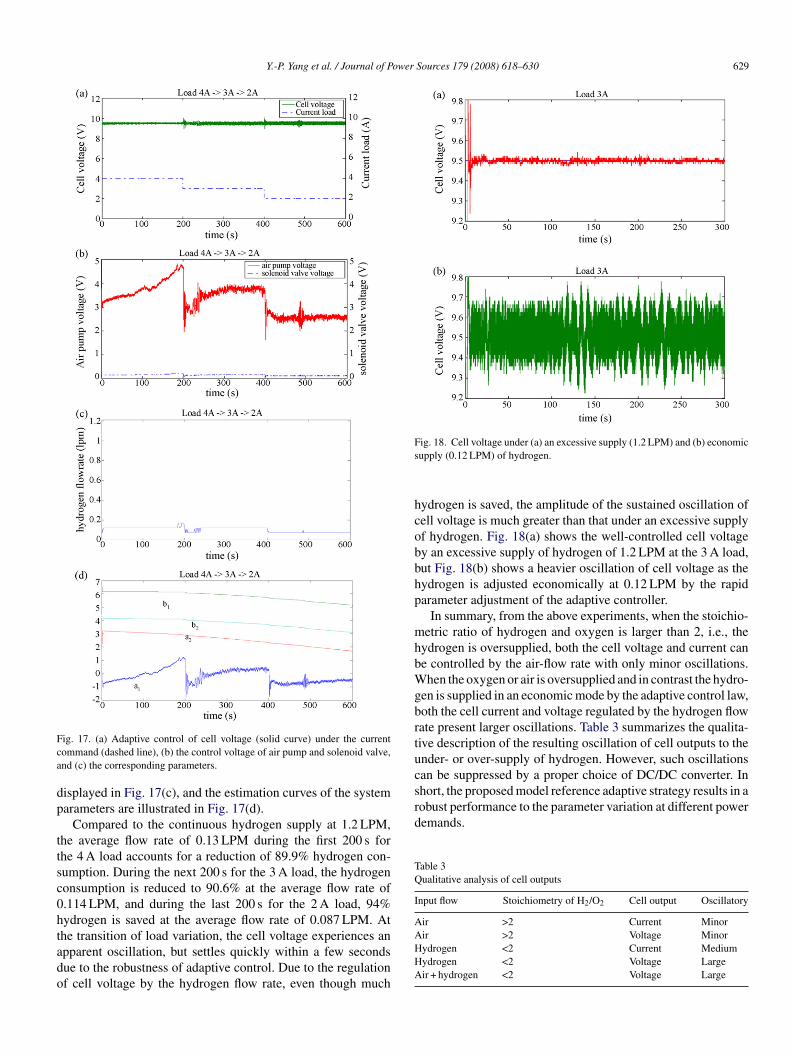
.5 V while the load current demand varies from 4 A throughA to 2 A at 200 and 400 s, as shown in Fig. 17(a). The adaptiveontrol law of voltages of the air pump and solenoid valve ishown in Fig. 17(b); the corresponding hydrogen flow rate is
Y.-P. Yang et al. / Journal of Power Sources 179 (2008) 618–630 629
Fca
dp
ttsc0htado
Fs
hcobbhp
mhbWgbrtucsrobust performance to the parameter variation at different powerdemands.
Table 3Qualitative analysis of cell outputs
Input flow Stoichiometry of H2/O2 Cell output Oscillatory
Air >2 Current Minor
ig. 17. (a) Adaptive control of cell voltage (solid curve) under the currentommand (dashed line), (b) the control voltage of air pump and solenoid valve,nd (c) the corresponding parameters.
isplayed in Fig. 17(c), and the estimation curves of the systemarameters are illustrated in Fig. 17(d).
Compared to the continuous hydrogen supply at 1.2 LPM,he average flow rate of 0.13 LPM during the first 200 s forhe 4 A load accounts for a reduction of 89.9% hydrogen con-umption. During the next 200 s for the 3 A load, the hydrogenonsumption is reduced to 90.6% at the average flow rate of.114 LPM, and during the last 200 s for the 2 A load, 94%ydrogen is saved at the average flow rate of 0.087 LPM. At
he transition of load variation, the cell voltage experiences anpparent oscillation, but settles quickly within a few secondsue to the robustness of adaptive control. Due to the regulationf cell voltage by the hydrogen flow rate, even though much
AHHA
ig. 18. Cell voltage under (a) an excessive supply (1.2 LPM) and (b) economicupply (0.12 LPM) of hydrogen.
ydrogen is saved, the amplitude of the sustained oscillation ofell voltage is much greater than that under an excessive supplyf hydrogen. Fig. 18(a) shows the well-controlled cell voltagey an excessive supply of hydrogen of 1.2 LPM at the 3 A load,ut Fig. 18(b) shows a heavier oscillation of cell voltage as theydrogen is adjusted economically at 0.12 LPM by the rapidarameter adjustment of the adaptive controller.
In summary, from the above experiments, when the stoichio-etric ratio of hydrogen and oxygen is larger than 2, i.e., the
ydrogen is oversupplied, both the cell voltage and current cane controlled by the air-flow rate with only minor oscillations.hen the oxygen or air is oversupplied and in contrast the hydro-
en is supplied in an economic mode by the adaptive control law,oth the cell current and voltage regulated by the hydrogen flowate present larger oscillations. Table 3 summarizes the qualita-ive description of the resulting oscillation of cell outputs to thender- or over-supply of hydrogen. However, such oscillationsan be suppressed by a proper choice of DC/DC converter. Inhort, the proposed model reference adaptive strategy results in a
ir >2 Voltage Minorydrogen <2 Current Mediumydrogen <2 Voltage Largeir + hydrogen <2 Voltage Large
6 ower
5
fsepttpdipmacianvtcmreottttswppapa
A
vCh
R
[
[
[
[
[
[[
[
[
[
[
[
[
[
30 Y.-P. Yang et al. / Journal of P
. Conclusion
Indirect model reference adaptive control has been success-ully applied to a low-power PEM fuel cell. For use in controlystems, the highly nonlinear, time-varying, distributed param-ter fuel cell stack of complex electrochemical reactions andhysics is approximated by a simple two-input two-output modelhat is described within subsystem blocks. These blocks describehe dynamic relationship between cell voltage and current out-uts and the hydrogen and air-flow rate inputs. By including theynamics of the air pump and solenoid valve, the correspond-ng transfer functions are identified off-line at certain operatingoints via a non-parametric frequency domain method. Theodel is subsequently reduced to an auto-regressive moving-
verage model for on-line parameter estimation in an adaptiveontrol loop. Experimental results show that the adaptive controls effective in regulating cell current and voltage by adjustingir and hydrogen flow rates in response to fuel cell and exter-al power demand perturbations. On–off control of the hydrogenalve is shown to reduce fuel consumption, which increases sys-em efficiency. It is noteworthy that the successful regulation ofell voltage by manipulation of the air pump and hydrogen valveay relieve DC/DC converters of demanding requirements for
egulating fluctuating cell voltage. Nevertheless, the model ref-rence adaptive control is applied under restricted conditions ofperation in this research; it is necessary to make more effortoward its robustness and generality to a class of fuel cell sys-ems. In addition, it is an important issue to include the water andhermal management in future research to monitor and controlhe humidity and temperature of reactants and the membraneo that the fuel cell can operate in a safe, efficient, and robustay with the proposed control strategy. It is expected that theroposed adaptive control can be easily extended to more com-lex multivariable control problems when more system statesre to be regulated, and could be applied to stationary and trans-ortation systems, as well as low- and high-power fuel cellpplications.
cknowledgments
The authors would like to thank Delta ElectronicsTM for pro-iding the portable PEMFC system and Mr. H.P. Chang in thehung Shan Institute of Science and Technology (CSIST) foris technical support for this paper.
[
[[
Sources 179 (2008) 618–630
eferences
[1] M.A.J. Cropper, S. Geiger, D.M. Jollie, J. Power Sources 131 (2004) 57–61.
[2] K. Astrom, E. Fontell, S. Virtanen, J. Power Sources 171 (2007) 46–54.[3] Y. Shao, G. Yin, Y. Gao, J. Power Sources 171 (2007) 558–566.[4] F. Mueller, J. Brouwer, S.G. Kang, H.-S. Kim, K.D. Min, J. Power Sources
163 (2) (2007) 814–829.[5] J.T. Pukrushpan, A.G. Stefannopoulou, H. Peng, IEEE Control Syst. Mag.
(2004) 30–46.[6] M. Ceraolo, C. Miulli, A. Pozio, J. Power Sources 113 (2003) 131–144.[7] J. Golbert, D.R. Lewin, J. Power Sources 135 (2004) 135–151.[8] P.R. Pathapati, X. Xue, J. Tang, Renew. Energy 30 (May) (2005) 1–22.[9] Y. Shan, S.Y. Choe, J. Power Sources 158 (1) (2006) 274–286.10] K.D. Min, J. Brouwer, J.S. Auckland, F. Mueller, G.S. Samuelsen,
Dynamic simulation of a stationary PEM fuel cell system, in: Proceed-ings of the 4th International Conference on Fuel Cell Science, Engineeringand Technology. June 19–21, 2006, Irvine, CA, ASME Paper FC2006-97039.
11] A. Paradkar, A. Davari, A. Feliachi, T. Biswas, J. Power Sources 128 (2004)218–230.
12] J.O. Schumacher, P. Gemmar, M. Denne, M. Zedda, M. Stueder, J. PowerSources 129 (2004) 143–151.
13] F. Jurado, J.R. Saenz, IEEE Trans. Energy Convers. 18 (June (2)) (2003)342–347.
14] M. Tekin, D. Hissel, M.C. Pera, J.M. Kauffmann, J. Power Sources 156 (1)(2006) 57–63.
15] C.H. Woo, J.B. Benziger, Chem. Eng. Sci. 62 (4) (2007) 957–968.16] R.T. Meyer, S. Revankar, A survey of PEM fuel cell system control models
and control developments, in: Proceedings of FuelCell06: The Fourth Inter-national Conference on Fuel Cell Science, Engineering and Technology.Irvine, California, June 19–21, 2006, Paper No. 97030.
17] R.N. Methekar, V. Prasad, R.D. Gudi, J. Power Sources 165 (1) (2007)152–170.
19] F.C. Wang, Y.P. Yang, C.W. Huang, H.P. Chang, H.T. Chen, J. PowerSources 164 (10 February (2)) (2007) 704–712.
20] R.F. Mann, J.C. Amphlett, M.A.I. Hooper, H.M. Jensen, B.A. Peppley, P.R.Roberge, J. Power Sources 86 (2000) 173–180.
21] S. Yerramalla, A. Davari, A. Feliachi, T. Biswas, J. Power Sources 124(2003) 104–113.
22] J.M. Correa, F.A. Farret, L.N. Canha, An analysis of the dynamic perfor-mance of proton exchange membrane fuel cells using an electrochemicalmodel, in: IECON’01, The 27th Annual Conference of the IEEE IndustrialElectronics Society, 2001, pp. 141–146.
23] M.A.R.S. Al-Baghdadi, H.A.K.S. Al-Janabi, Renew. Energy 32 (7) (2007)1077–1101.
24] G.F. Franklin, J.D. Powell, A. Emami-Naeini, Feedback Control ofDynamic Systems, 5th edition, Pearson Prentice Hall, 2006.
25] R. von Helmolt, U. Eberle, J. Power Sources 165 (2007) 833–843.26] G.C. Goodwin, K.S. Sin, Adaptive Filtering Prediction and Control,