QUANTITATIVE METHODS IN ECONOMICS Vol. XII, No. 1, 2011, pp. 1–13

AN APPLICATION OF RADAR CHARTS TO GEOMETRICAL MEASURES OF STRUCTURES’ OF CONFORMABILITY

Zbigniew Binderman, Bolesław Borkowski Department of Econometrics and Statistics,

Warsaw University of Live Sciences – SGGW e-mails: zbigniew_binderman@sggw.pl; boleslaw_borkowski@sggw.pl

Wiesław Szczesny Department of Informatics, Warsaw University of Live Sciences – SGGW

e-mail: wieslaw_szczesny@sggw.pl

Abstract: In the following work we presented a method of using radar charts to calculate measures of conformability of two objects according to formulas given by, among others, Dice, Jaccard, Tanimoto and Tversky. This method incorporates another one presented by the authors of this study [Binderman, Borkowski, Szczesny 2010]. Presented methods can be also utilized to define similarities between given objects, as well as to order and group objects. Measures described in this work satisfy the condition of stability as they do not depend on the order of studied features.

Key words: radar method, radar measure of conformability, Dice’s, Jaccard’s measure of similarity, synthetic measures, classification, cluster analysis.

CONSTRUCTION OF RADAR MEASURES OF CONFORMABILITY

In previous works authors used methods that have a simple interpretation in the form of a radar chart to order, classify and measure similarity of objects [Binderman, Borkowski, Szczesny 2008, 2009, 2009a, 2010, 2010a, b, c, d, Binderman, Szczesny 2009, 2011, Binderman 2009, 2009a]. Those methods do not depend on the way the features of a given object are ordered. In the following work authors attempted to utilize those methods in other, widely known means of measuring similarity between two objects. Comparing structures of objects is chosen here as an example. Coefficients of Jaccard, Dice and Tanimoto, Tversky index and cosine similarity are all exemplary geometrical measures of similarity.

2 Zbigniew Binderman, Bolesław Borkowski, Wiesław Szczesny

The methods presented here may seem numerically complicated but in the age of computers this problem is of little significance.

Numerous studies conducted in many different fields of science: economics, statistics, computer science, chemistry, biology, ecology, psychology, culture and tourism have proven the usefulness of those methods [Binderman 2009a, Binderman, Borkowski, Szczesny 2010b, c, Ciok, Kowalczyk, Pleszczyńska, Szczesny 1995, Deza E., Deza M.M. 2006, Duda, Hart, Stork 2000, Gordon 1999, Hubalek 1982, Kukuła 2000, 2010, Legendre P., Legendre L. 1998, Monev 2004, Szczesny 2002, Tan, Steinbach, Kumar 2006, Warrens 2008].

Let Q and P be two objects that are described by a set of n (n>2) features. Assume that objects Q and P are described by two vectors ,n

+∈ℜx, y where:

1 2 1 2

1 1

1 20and

1 1

, ,...,( , ,..., ), ( , ,..., ); , ;

, .

n n i i

n n

i ii i

i nx x x y y y x y

x y= =

== = ≥

= =∑ ∑

x y

In order to graphically represent the methods we inscribe a regular n-gon into a unit circle (with a radius of 1) with a centre in the origin of a polar coordinate system 0uv and we will connect the vertices of this n-gon with the origin of the coordinate system. Thus, one constructs line segments of length 1, we will denote, in sequence, O1,O2,...,0n, starting, for definitiveness, with the line segment covering w axis. Assume that at least two coordinates of each of the vectors x and y are non-zero. Because features of objects x and y take on values from an interval <0,1>, that is 0≤x≤1 ≡ 0≤xi≤1, 0≤y≤1 ≡ 0≤yi≤1, i=1,2,...n, where 0:=(0,0,...,0), 1:=(1,1,...,1), we can represent the values of those features as a radar chart. To do so, let xi (yi) denote those points on the 0i axis that came into being by intersecting the 0i axis with a circle with the centre at the origin of the coordinate system and radius of xi (yi), i=1,2,...,n. By connecting the points: x1 with x2, x2 with x3, ..., xn with x1 (y1 with y2, y2 with y3, ..., yn with y1) we get n-gons SQ and SP, where its areas ⎢SQ⎢ and ⎢SP⎢, are given by formulas:

i i 1 i i 1 n 1 1

i i 1 i i 1 n 1 1

n n

Qi 1 i 1n n

Pi 1 i 1

2 2:

n n

2 2:

n n

12

12

1S sin sin , gdzie ,2

1S sin sin , gdzie .2

x x x x x

y y y y y

S x

S y

+ + +

+ + +

= =

= =

π π= =

π π= =

= =

= =

∑ ∑

∑ ∑

x

y

(1)

The formula for the area of the intersection of those n-gons, which we will denote by :S S S∩ = ∩x y x y has a more complicated form. Its form and detailed determination can be found in [Binderman, Borkowski, Szczesny 2010]. Using those formulae we can denote the area of the union of n-gons Sx and Sy as

An application of radar charts … 3

S S S S S S ,∪ = + − ∩x y x y x y (2)

where the areas x y,S S are defined by formulae (1).

Figure 1 presents two graphical illustrations of vectors x=(0,2, 0,2, 0,3, 0,15, 0,1, 0,05) and y =(0,15, 0,15, 0,2, 0,25, 0,15, 0,1) that describe two exemplary demographical structures (for age ranges: 0-14, 15-24, 25-49, 50-64, 65-79, >80), while Fig. 1A and 1B differ only by the order of axes (meaning the permutation of the coordinates).

Fig. 1. Radar charts for vectors x and y, which coordinates present two exemplary demographical structures, by different ordering of axes.

A

00,05

0,10,15

0,20,25

0,30-14

15-24

25-49

50-64

65-79

>80

B

00,05

0,1

0,150,2

0,25

0,30-14

25-49

15-24

65-79

50-64

>80

Source: own work

From the figure it is clear that areas of n-gons x y,S S and their unions on figures

1A and 1B differ in size. They are: 0,076; 0,074; 0,051 and 0,075; 0,069; 0,047, respectively.

In works [Binderman Borkowski, Szczesny 2008, 2010] authors proposed a measure of conformability of objects that uses a geometrical interpretation in the form of radar charts and is defined as follows:

for 3

for 4

3, ( )

S Sn

S Sn

R

∩=

σ

∩≥

ω

=

⎧⎪⎪⎨⎪⎪⎩

x y

xy

xy

x y

xy

4 Zbigniew Binderman, Bolesław Borkowski, Wiesław Szczesny

where

gdy 0 gdy 0

1 gdy 0 1 gdy 0

> >

= =

⎧ ⎧⎪ ⎪⎨ ⎨⎪ ⎪⎩ ⎩

σ = ω =x y x y x y x y

xy xyx y x y

min( , ) max( , ).: , :

S S S S S S S S

S S S S

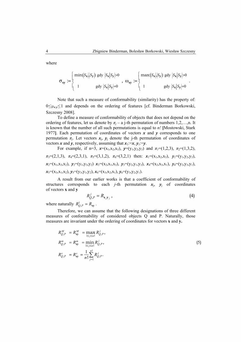
Note that such a measure of conformability (similarity) has the property of:

0≤μx.y≤1 and depends on the ordering of features [cf. Binderman Borkowski, Szczesny 2008].

To define a measure of conformability of objects that does not depend on the ordering of features, let us denote by πj – a j-th permutation of numbers 1,2,…,n. It is known that the number of all such permutations is equal to n! [Mostowski, Stark 1977]. Each permutation of coordinates of vectors x and y corresponds to one permutation πj. Let vectors xj, yj denote the j-th permutation of coordinates of vectors x and y, respectively, assuming that x1:=x, y1:=y.

For example, if n=3, x=(x1,x2,x3), y=(y1,y2,y3) and π1=(1,2,3), π2=(1,3,2),

π3=(2,1,3), π4=(2,3,1), π5=(3,1,2), π6=(3,2,1) then: x1=(x1,x2,x3), y1=(y1,y2,y3),

x2=(x1,x3,x2), y2=(y1,y3,y2) x3=(x2,x1,x3), y3=(y2,y1,y3), x4=(x2,x3,x1), y4=(y2,y3,y1),

x5=(x3,x1,x2), y5=(y3,y1,y2), x6=(x3,x2,x1), y6=(y3,y2,y1).

A result from our earlier works is that a coefficient of conformability of structures corresponds to each j-th permutation xj, yj of coordinates of vectors x and y

4, , ( )j j

jQ PR R= x y

where naturally 1,Q PR R= xy .

Therefore, we can assume that the following designations of three different measures of conformability of considered objects Q and P. Naturally, those measures are invariant under the ordering of coordinates for vectors x and y.

1

1

1

5

1

, ,!

, ,!

!

, ,

max ,

min , ( )

.!

jM MQ P Q Pj n

jm mQ P Q Pj n

njs s

Q P Q Pj

R R R

R R R

R R Rn

≤ ≤

≤ ≤

=

= =

= =

= = ∑

xy

xy

xy

An application of radar charts … 5

Other well-known in literature techniques that use geometrical interpretations, such as radar charts, may be used to compare two structures 1 2 1 2= =x y( , ,..., ), ( , ,..., )n nx x x y y y . Most well known among them are:

cosine similarity [Deza, Deza 2006]

S Sfor S S 0

S Sc ,

0 for S S 0

⎧ ∩⎪ >⎪= ⎨⎪

=⎪⎩

x yx y

xy x y

x y

(6)

Jaccard coefficient [Jaccard 1901, 1902, 1908]

S Sfor S S 0

S SJ ,

0 for S S 0

⎧ ∩⎪ >⎪ ∪= ⎨⎪

=⎪⎩

x yx y

xy x y

x y

(7)

Dice’s coefficient [Dice 1945]

2 S Sfor S S 0

S SD ,

0 for S S 0

⎧ ∩⎪ >⎪ += ⎨⎪

=⎪⎩

x yx y

xy x y

x y

(8)

Tanimoto coefficient [Tanimoto 1957, 1959]

y

S Sfor S S 0

S S S S ,

0 for S S 0

⎧ ∩⎪ >⎪ + − ∩= ⎨⎪

=⎪⎩

x yx y

xy x y x

x y

T (9)

6 Zbigniew Binderman, Bolesław Borkowski, Wiesław Szczesny

Tversky index [Tversky 1957]

y ,

S Sfor S S 0

S S S \ S S \ ST 0.

0 for S S 0

βα α β

⎧ ∩⎪ >⎪ ∩ + += ≥⎨⎪

=⎪⎩

x yx y

xy x x y y x

x y

(10)

Let us note that if in the above formula the coefficients fulfill α=β=1 then

we get Tanimoto’s formula and if α=β= 1

2 then we get Dice’s formula. Here and in

the sequel we shall assume that α=β= 1

4.

Note that the defined above measures of similarity, take a value between [0, 1], are dependent on the ordering of features in case once represents the object by a radar chart.

Another simple way of visualizing the structure 1 2=x ( , ,..., )nx x x is a bar graph, in which each coordinate is represented as a rectangle of width 1 and height xi (for i=1,…,n). The area of such graph is equal to 1 and one of the most popular indicators of similarity of two structures 1 2=x ( , ,..., )nx x x and 1 2=y ( , ,..., )ny y y is defined as [Malina 2004]:

1: min( , ) , (11)

n

i ii

W x y=

=∑xy

It is clear that its value is independent of the ordering of features and, in the case of such graphical representation of structure, takes a value identical to the values of coefficients defined in (6) and (8).

In every situation when the indicator of similarity of two structures that uses

a graphical interpretation is not invariant under the permutation of coordinates, we may modify its definition, in a way shown above (see formula (5)). Thus, to define a measure of conformability that would be independent of the ordering of features, let us denote by pj – the j-th permutation of numbers 1,2,…,n. Naturally, each permutation of coordinates of vectors x and y corresponds to one permutation pj. Let vectors xj, yj denote j-th permutation of coordinates of vectors x and y, respectively. Assume that x1=x, y1=y, for each j-th permutation xj, yj of coordinates of vectors x and y corresponds a coefficient of conformability of structures

12, , ( )j j

jQ P cc = x y

An application of radar charts … 7

where naturally 1,Q Pc c= xy , and the cosine similarity xyc is defined as in formula

(6). With regard to the above, let us assume the following definitions of three

different measures of conformability for objects Q and P

1

1

1

13

1

, ,!

, ,!

!

, ,

max ,

min , ( )

.!

jM MQ P Q Pj n

jm mQ P Q Pj n

njs s

Q P Q Pj

c c c

c c c

c c cn

≤ ≤

≤ ≤

=

= =

= =

= = ∑

x,y

x,y

x,y

In a similar manner we can define other coefficients

M m s M m s M m s M m sJ , J , J ;D , D , D ; , , ;T ,T Txy xy xy xy xy xy xy xy xy xy xy xyT T T . In order to demonstrate the presented above method of comparing

structures, let us consider a simple example.

Example 1. Let 1 1 1 1 1, , , ,

2 2 3 3 30 , .⎛ ⎞ ⎛ ⎞= = = =⎜ ⎟ ⎜ ⎟

⎝ ⎠ ⎝ ⎠x yQ R Let us assume the

following denotations:

1 4 2 5 3 6

1 2 3 4 5 6

1 1 1 1: : , : : ,0, , : : 0, , ,2 2 2 2

: : : : : .

⎛ ⎞ ⎛ ⎞= = = = = =⎜ ⎟ ⎜ ⎟⎝ ⎠ ⎝ ⎠

= = = = = =

x x x x x x x

y y y y y y y

Thus we have:

1 1 1 2 3 1 1 1 2 3sin , 3 sin ,2 2 2 3 16 2 3 3 3 12

1 1 1 2 3 17 3sin , ,2 3 3 3 36 144

3 3 2 , dla 1,2,...,6.36 16 3

/

i i

i i i i

i i

S S

S S S S

R i

= = = =

∩ = = ∪ =

= = =

x y

x y x y

x y

π π

π

8 Zbigniew Binderman, Bolesław Borkowski, Wiesław Szczesny

So 2 0 6663 ~ ,M m sR R R= = = =x,y x,y x,y , where coefficients , , ,, ,M s mQ P Q P Q PR R R

are defined as in formulae (5). It can be easily verified that coefficients of conformability of structures: cosine (formula (13)), Jaccard, Dice’s are equal to:

0 385 0 236 0 381= = = = = = = = =x,y x,y x,y x,y x,y x,y x,y x,y x,y, ; , ; , .M m s M m s M m sc c c J J J D D D

Note that

0 620 0 486 0 617= = =x,y x,y x,y, ; , ; , .M M Mc J D

It is also noteworthy that in this case the coefficient of conformability of structures

(defined by formula (11)) is 1 1 20 .3 3 3

W = + + =xy The value of the coefficient

define by formula (7) or (9) that uses an interpretation of the structure as a bar graph is equal to 0,5 =0,6(6)/1,3(3).

The above example shows that measures of similarity of two objects calculated by different methods (e.g. a method that includes the manner of the graphical representation of the structure or a method of normalizing, which, when applied, causes the measure of the area of the union of faces to take a value between [0, 1]), can be significantly different. A single measure of similarity of objects can be far from optimal in the understanding of a given expert. Furthermore, experts can disagree on the meanings of individual measures. Thus it is safer to use, in the analysis of structures, a measure that is, for example, an average of several different measures of similarity [see: Breiman 1994].

EMPIRICAL RESULTS

In order to verify the approach described in the previous section, we present an evaluation of the size of changes in demographical structures of European countries between the years 1999 and 2000, using the discussed above coefficients.

The following Tables 1 and 2 contain values of indicators evaluating the change of demographical structures for 27 countries between years 1999 and 2010; with an indication what position they occupied in the ranking of values of individual measures as well as two partitions of countries into 4 groups (columns C1 and C2). The partition is made based on the values of indicator M (arithmetic mean of values of indicators R, C, J, D and T) and indicator W, while the thresholds were defined as: A-d, A, A+d, where A denotes an average and d – standard deviation.

An application of radar charts … 9

Table 1. Values and rankings of indicators evaluating the similarity of demographical structures of 27 European countries in the years 1999 and 2010. Indicators are defined on the grounds of formulas: R - (3), C - (6), J - (7), D - (8), T-(10), M=(R+C+J+D+T)/5, W - (11) for the following ordering of age ranges: 0-14, 15-24, 25-49, 50-64, 65-79, >80. The last two columns contain information about the partition into 4 groups, according to values of indicators M and W, respectively.

No. country R C J D T M W R C J D T M W C1 C21 Austria 0,9676 0,9536 0,9110 0,9534 0,9762 0,9524 0,9630 5 5 5 5 5 5 6 1 12 Belgium 0,9616 0,9427 0,8913 0,9425 0,9704 0,9417 0,9590 9 7 7 7 7 7 8 2 23 Bulgaria 0,9455 0,9038 0,8243 0,9037 0,9494 0,9054 0,9480 14 15 15 15 15 15 11 3 24 Cyprus 0,9319 0,8967 0,8120 0,8963 0,9453 0,8964 0,9320 21 16 16 16 16 17 24 3 45 Czech Republic 0,9347 0,8776 0,7818 0,8776 0,9348 0,8813 0,9370 19 23 23 23 23 23 21 3 36 Denmark 0,9781 0,9606 0,9242 0,9606 0,9799 0,9607 0,9700 1 3 3 3 3 2 3 1 17 Estonia 0,9634 0,9438 0,8933 0,9437 0,9710 0,9430 0,9600 6 6 6 6 6 6 7 2 28 Finland 0,9469 0,9123 0,8385 0,9121 0,9540 0,9128 0,9400 13 14 14 14 14 14 19 2 39 France 0,9504 0,9180 0,8482 0,9178 0,9572 0,9183 0,9480 12 13 13 13 13 13 11 2 2

10 Germany 0,9624 0,9340 0,8762 0,9340 0,9659 0,9345 0,9470 7 10 10 10 10 10 15 2 311 Greece 0,9364 0,8900 0,8016 0,8899 0,9417 0,8919 0,9450 17 18 18 18 18 18 16 3 312 Hungary 0,9441 0,8950 0,8100 0,8950 0,9446 0,8978 0,9480 16 17 17 17 17 16 10 3 213 Ireland 0,9225 0,8754 0,7779 0,8751 0,9334 0,8769 0,9400 25 24 24 24 24 24 19 4 314 Italy 0,9620 0,9346 0,8771 0,9345 0,9662 0,9349 0,9710 8 9 9 9 9 9 2 2 115 Latvia 0,9587 0,9386 0,8839 0,9384 0,9682 0,9375 0,9520 10 8 8 8 8 8 9 2 216 Lithuania 0,9451 0,9239 0,8577 0,9234 0,9602 0,9220 0,9440 15 12 12 12 12 12 17 2 317 Luxembourg 0,9716 0,9650 0,9318 0,9647 0,9820 0,9630 0,9720 2 1 1 1 1 1 1 1 118 Malta 0,9263 0,8809 0,7867 0,8806 0,9365 0,8822 0,9260 24 22 22 22 22 22 25 3 419 Netherlands 0,9531 0,9276 0,8646 0,9274 0,9623 0,9270 0,9470 11 11 11 11 11 11 13 2 320 Poland 0,9061 0,8464 0,7331 0,8460 0,9166 0,8497 0,9220 27 27 27 27 27 27 26 4 421 Portugal 0,9357 0,8873 0,7973 0,8872 0,9402 0,8895 0,9470 18 19 19 19 19 19 13 3 322 Romania 0,9346 0,8820 0,7888 0,8820 0,9373 0,8849 0,9360 20 21 21 21 21 21 22 3 323 Slovakia 0,9131 0,8531 0,7435 0,8529 0,9206 0,8566 0,9220 26 26 26 26 26 26 27 4 424 Slovenia 0,9288 0,8667 0,7647 0,8667 0,9286 0,8711 0,9330 23 25 25 25 25 25 23 4 425 Spain 0,9299 0,8860 0,7949 0,8857 0,9394 0,8872 0,9440 22 20 20 20 20 20 17 3 326 Sweden 0,9689 0,9594 0,9215 0,9592 0,9792 0,9576 0,9670 4 4 4 4 4 4 5 1 127 United Kingdom 0,9700 0,9625 0,9272 0,9622 0,9808 0,9605 0,9690 3 2 2 2 2 3 4 1 1

Source: own work

Note that each of the first 5 indicators presented in Table 1, has an identical geometrical interpretation of similarity of structures, an intersection of two hexagons that represent those structures. They differ only by the method used to normalize that area, so that the value of the indicator of similarity is between [0, 1]. That is why all the indicators, with the exception of indicator R, they give the same ordering of European countries, according to the similarity of structures for the years 1999 and 2010. Small differences are visible only in the case of indicator R. The results do not change if we modify the indicator so that its value is independent of the ordering of coordinates of the vector representing the structure (see. Table 2). On the other hand, differences between the ordering by the value of indicator W (based on a different visualization of structures that the rest), and the

10 Zbigniew Binderman, Bolesław Borkowski, Wiesław Szczesny

ordering by the value of indicator M are noticeable. Even more so in the last two columns of Table 2, which represent the partition of countries into 4 groups, according to the similarity of structures for years 1999 and 2010. In case of Spain, we can observe a substantial difference in the assignment to a group depending on the used indicator.

Table 2. Description is similar to that of Table 1. The calculations of individual indicators where performed based on the first formulas (maximum) from (5), (13) and analogous modifications freeing the value of an indicator from the ordering of coordinates of a vector describing a given structure.

No. country RM CM JM DM TM MMW RM CM JM DM TM MM

W C1 C21 Austria 0,9737 0,9572 0,9177 0,9571 0,9781 0,9567 0,9630 6 6 6 6 6 6 6 1 12 Belgium 0,9671 0,9427 0,8913 0,9425 0,9704 0,9428 0,9590 10 9 9 9 9 10 8 1 23 Bulgaria 0,9658 0,9360 0,8796 0,9360 0,9669 0,9369 0,9480 13 15 15 15 15 15 11 2 24 Cyprus 0,9592 0,9239 0,8575 0,9233 0,9601 0,9248 0,9320 19 20 21 21 21 19 24 2 45 Czech Republic 0,9582 0,9216 0,8545 0,9215 0,9592 0,9230 0,9370 21 22 22 22 22 22 21 2 36 Denmark 0,9812 0,9658 0,9338 0,9658 0,9826 0,9658 0,9700 2 2 2 2 2 2 3 1 17 Estonia 0,9702 0,9512 0,9066 0,9510 0,9749 0,9508 0,9600 8 7 7 7 7 7 7 1 28 Finland 0,9605 0,9294 0,8673 0,9290 0,9632 0,9299 0,9400 18 18 18 18 18 18 19 2 39 France 0,9590 0,9234 0,8577 0,9234 0,9602 0,9247 0,9480 20 21 20 20 20 20 11 2 2

10 Germany 0,9668 0,9386 0,8842 0,9385 0,9683 0,9393 0,9470 11 12 12 12 12 12 15 1 311 Greece 0,9629 0,9316 0,8718 0,9315 0,9646 0,9325 0,9450 17 17 17 17 17 17 16 2 312 Hungary 0,9635 0,9318 0,8722 0,9317 0,9647 0,9328 0,9480 15 16 16 16 16 16 10 2 213 Ireland 0,9665 0,9429 0,8918 0,9428 0,9705 0,9429 0,9400 12 8 8 8 8 9 19 1 314 Italy 0,9804 0,9669 0,9357 0,9668 0,9831 0,9666 0,9710 3 1 1 1 1 1 2 1 115 Latvia 0,9632 0,9416 0,8890 0,9412 0,9697 0,9410 0,9520 16 11 11 11 11 11 9 1 216 Lithuania 0,9527 0,9254 0,8598 0,9246 0,9608 0,9247 0,9440 24 19 19 19 19 21 17 2 317 Luxembourg 0,9791 0,9650 0,9318 0,9647 0,9820 0,9645 0,9720 4 3 4 4 4 4 1 1 118 Malta 0,9491 0,9097 0,8340 0,9095 0,9526 0,9110 0,9260 25 26 26 26 26 26 25 3 419 Netherlands 0,9653 0,9379 0,8831 0,9379 0,9680 0,9384 0,9470 14 13 13 13 13 14 13 1 320 Poland 0,9468 0,9031 0,8233 0,9031 0,9491 0,9051 0,9220 27 27 27 27 27 27 26 3 421 Portugal 0,9680 0,9376 0,8826 0,9376 0,9678 0,9387 0,9470 9 14 14 14 14 13 13 1 322 Romania 0,9548 0,9172 0,8470 0,9171 0,9568 0,9186 0,9360 22 23 23 23 23 23 22 3 323 Slovakia 0,9544 0,9118 0,8378 0,9118 0,9538 0,9139 0,9220 23 25 25 25 25 25 27 3 424 Slovenia 0,9482 0,9151 0,8416 0,9140 0,9551 0,9148 0,9330 26 24 24 24 24 24 23 3 425 Spain 0,9705 0,9425 0,8913 0,9425 0,9704 0,9434 0,9440 7 10 10 10 10 8 17 1 326 Sweden 0,9814 0,9649 0,9322 0,9649 0,9822 0,9651 0,9670 1 4 3 3 3 3 5 1 127 United Kingdom 0,9790 0,9634 0,9293 0,9634 0,9813 0,9633 0,9690 5 5 5 5 5 5 4 1 1

Source: own work

Tables 1 and 2 show that the greatest stability of the demographical structure between 1999 and 2010 was possessed by: Austria, Denmark, Luxembourg, Sweden and United Kingdom. On the other hand, the greatest changes were observed in: Cyprus, Malta, Poland, Slovakia and Slovenia. The greatest change occurred in Poland, and the smallest one in Luxembourg.

An application of radar charts … 11

SUMMARY

Means for defining the values of indicators of similarity that use geometrical interpretations in the form of a value of an area and are described in this work can also be used in other geometrical ways of studying the similarity of structures as well as objects. These ways are an example of applying geometrical methods that are introduced by the authors using radar charts [Binderman, Borkowski, Szczesny 2008, 2010]. The empirical analysis shows that when structures are not subject to large changes then the values of individual indicators, based on the same geometrical interpretation, they order the structures similarly. However, if we change the way of visualizing the similarity (the geometrical interpretation) then we see changes in ordering. That is the reason why it is advisable to use several different indicators that use different means of visualization.

Furthermore, it is worth noting that by using geometrical interpretation as a basis to construct an indicator of similarity we can obtain an indicator that is very sensitive to changes in the ordering of coordinates of a vector that numerically represents a given structure. In practice there may be situations in which a researcher desires such quality in an indicator so it may visibly highlight even small differences between structures, but for a given ordering of their components. However, one needs to remember that methods of constructing indicators of similarity that use a geometrical interpretation are often applied mainly because of the ease of visualization of multidimensional data. Then an unseasoned researcher may misuse them. It must be highlighted that indicators based solely on those illustrations do not satisfy – often posed in the literature on this subject – the basic requirement of stability of the used method [see Jackson 1970], that means the independence of the ordering of features. Techniques presented by the authors show how a definition of an indicator must be modified (the method of measurement) to remove this flaw. Techniques that were pointed out may seem numerically complex; nevertheless, in the age of computers that problem became insignificant. On the other hand, this simple and stable empirical example shows that by applying modifications, that is making the measurement of similarity independent of the ordering of individual components of the structure, we obtain different results (see Tables 1 and 2, e.g., Spain).

The measurement of similarity of structures based on geometrical interpretation becomes even more complicated when a researcher is interested in changes that occurred in a given structures during the whole studied period and not only between the beginning and the end of the sample. Further works on this subject can be found in the work Binderman and Szczesny 2011.

12 Zbigniew Binderman, Bolesław Borkowski, Wiesław Szczesny

REFERENCES

Binderman Z., Borkowski B., Szczesny W. (2008) O pewnej metodzie porządkowania obiektów na przykładzie regionalnego zróżnicowania rolnictwa, Metody ilościowe w badaniach ekonomicznych, IX, wyd. SGGW, 39-48.

Binderman Z., Borkowski B., Szczesny W (2009) O pewnych metodach porządkowych w analizie polskiego rolnictwa wykorzystujących funkcje użyteczności, Roczniki Nauk Rolniczych PAN, Seria G, Ekonomika Rolnictwa , T. 96, z. 2, 77-90.

Binderman Z., Borkowski B., Szczesny W. (2009a) Tendencies in changes of regional differentiation of farms structure and area Quantitative methods in regional and sectored analysis / sc. ed. D. Witkowska D., Łatuszyńska M., U.S., Szczecin, 33-50.

Binderman Z., Borkowski B., Szczesny W. (2010) Radar measures of structures’ conformabilty, Quantitative methods in economy, v. XI, No.1, 45-59.

Binderman Z., Borkowski B., Szczesny W. (2010a) The tendencies in regional differentiation changes of agricultural production structure in Poland, Quantitative methods in regional and sectored analysis , U.S., Szczecin, 67-103.

Binderman Z., Borkowski B., Szczesny W. (2010b) Wykorzystanie metod geometrycznych do analizy regionalnego zróżnicowania kultury na wsi, Seria T. XII, z. 5, 25-31.

Binderman, Z., Borkowski B., Szczesny W. (2010c) Regionalne zróżnicowanie turystyki w Polsce w latach 2002–2008, Oeconomia 9 (3) 71-82.

Binderman Z., Borkowski B., Szczesny W. (2010d) Regionalnego zróżnicowanie kultury między wsią a miastem w latach 2003-2008, Między dawnym a nowym – na szlakach humanizmu, wyd. SGGW, 345-360.

Binderman Z., Szczesny W. (2009) Arrange methods of tradesmen of software with a help of graphic representations Computer algebra systems in teaching and research, Siedlce, Wyd. WSFiZ, 117-131.

Binderman Z., Szczesny W., (2011) Comparative Analysis of Computer Techniques for Visualization Multidimensional Data, Computer algebra systems in teaching and research, Siedlce, wyd. Collegium Mazovia, 243-254.

Binderman Z. (2009) Syntetyczne mierniki elastyczności przedsiębiorstw, Kwartalnik Prace i Materiały Wydziału Zarządzania Uniwersytetu Gdańskiego, nr 4/2, 257-268.

Binderman, Z. (2009a) Ocena regionalnego zróżnicowania kultury i turystyki w Polsce w 2007 roku Roczniki Wydziału Nauk Humanistycznych, SGGW, T XII, 335-351.

Borkowski B., Szczesny W. (2002) Metody taksonomiczne w badaniach przestrzennego zróżnicowania rolnictwa. Warszawa, RNR, Seria G, T 89, z. 2. 42-53.

Breiman L. (1994) Bagging predictors, Technical Report 420, Departament of Statistics, University of California, CA, USA, September 1994.

Ciok A., Kowalczyk T., Pleszczyńska E., Szczesny W. (1995) Algorithms of grade correspondence-cluster analysis. The Collected Papers on Theoretical and Aplied Computer Science, 7, 5-22.

Deza E., Deza M.M. (2006) Dictionary of Distances, Elsevier. Dice Lee R. (1945) Measures of the Amount of Ecologic Association Between Species,

Ecology, Ecological Society of America, Vol. 26, No. 3, 297-302.

An application of radar charts … 13

Duda R. O., Hart P. E., Stork D. G. (2000) Pattern Classification. John Wiley & Sons, Inc., 2nd ed.

Gordon, A.D. (1999) Classification, 2nd edition, London-New York. Hubalek Z. (1982) Coefficients of Association and Similarity, Based on Binary (Presence-

Absence) Data: An Evaluation, Biological Reviews, Vol.57-4, 669-689. Jaccard P. (1901) Étude comparative de la distribution florale dans une portion des Alpes et

des Jura. Bulletin del la Société Vaudoise des Sciences Naturelles 37, 547-579. Jaccard, P. (1902) Lois de distribution florale dans la zone alpine. Bull. Soc. Vaud. Sci.

Nat. 38, 69-130. Jaccard, P. (1908) Nouvel les recherches sur la distribution floral e. Bull. Soc. Vaud. Sci.

Nat. 44, 223-270. Jackson D. M. (1970) The stability of classifications of binary attribute data, Technical

Report 70-65, Cornell University, 1-13. Kukuła K. (2000) Metoda unitaryzacji zerowej, PWN, Warszawa. Kukuła K. (red) (2010) Statystyczne studium struktury agrarnej w Polsce, PWN,

Warszawa. Legendre P., Legendre L. (1998) Numerical Ecology, Second English Edition Ed., Elsevier. Malina A. (2004) Wielowymiarowa analiza przestrzennego zróżnicowania struktury

gospodarki Polski według województw. AE, Seria Monografie nr 162, Kraków. Monev V. (2004) Introduction to Similarity Searching in Chemistry, MATCH Commun.

Math. Comput. Chem. 51, 7-38. Mostowski A., Stark M.: Elementy algebry wyższej, PWN, Warszawa. Szczesny W. (2002) Grade correspondence analysis applied to contingency tables and

questionnaire data, Intelligent Data Analysis, vol. 6, 17-51. Tan P., Steinbach M., Kumar V. (2006) Introduction to Data Mining, Pearson Education,

Inc. Tanimoto, T.T. (1957) IBM Internal Report 17th Nov. 1957 Tanimoto T.T. (1959) An Elementary Mathematical Theory of Classification and

Prediction, IBM Program IBCFL. Tversky A. (1957) Features of similarity. Psychological Review, 84(4) 327-352. Warrens M. J. (2008) On Association Coefficients for 2×2 Tables and Properties that do

not depend on the Marginal Distributions, Psychometrika Vol. 73, n. 4, 777–789.

14 Zbigniew Binderman, Bolesław Borkowski, Wiesław Szczesny