PROCEEDINGS, Thirty-Ninth Workshop on Geothermal Reservoir Engineering Stanford University, Stanford, California, February 24-26, 2014 SGP-TR-202

1

An Approach for Investigation of Geochemical Rock-Fluid Interactions

Carina Bringedal, Inga Berre and Florin A. Radu

Department of Mathematics, University of Bergen

P.O. Box 7800, 5020 Bergen, Norway

carina.bringedal@math.uib.no

Keywords: Porosity changes, solute transport, finite volume method, mineral precipitation/dissolution

ABSTRACT Geochemistry has a substantial impact in exploiting of geothermal systems. When water is injected in a geothermal reservoir, the injected water and in-situ brine have different temperatures and chemical compositions and will flow through highly heterogeneous regions where the rock has varying chemical properties and where temperature and flow regimes can alter significantly.

As a consequence of flow and geochemical reactions, composition of reservoir fluids as well as reservoir rock properties will develop dynamically with time. Minerals dissolving and precipitating onto the reservoir matrix, can change the porosity and hence the permeability of the system substantially. Mineral solubility can change by the cooling of the rock by the injected water as well as by the injected water having a different salt content than the in-situ brine. The interaction between altering temperature, solute transport with mineral dissolution and precipitation, and fluid flow is highly coupled and challenging to model appropriately as the relevant physical processes jointly affect each other. The effect of changing porosity through the production period of the geothermal reservoir, may have severe impacts on operating conditions, as pores may close and block flow paths, or new pores may open to create enhanced flow conditions.

We propose an approach that models all three processes on a relevant time scale. The considered mathematical and corresponding overall numerical solution strategy enables us to investigate the coupling between flow, geochemical and thermal effects, as well as to develop tailored numerical approaches.

1. INTRODUCTION In a geothermal reservoir used for electricity production where cold fluid is injected into the subsurface through one or several injection wells and warmer fluid is produced from one or several production wells, the properties of the subsurface rock is highly important. Too low permeability will result in a too small volume flux of warm fluid being produced, while a too high permeability can cause the injected fluid to flow too fast through the reservoir and not gaining enough heat before being produced. The initial permeability and the location of the wells are therefore important, but how the permeability can change because of porosity changes due to chemical reactions should also be considered.

The subsurface rock consists of minerals that can dissolve into the saturating fluid. For a mineral dissolution or precipitation process to have a notable effect on the porosity (and permeability), large instances of the mineral or of the involved ions are necessary, and the chemical reaction must occur at a timescale relevant for geothermal energy. Moore et al (1982) tested through experiments how the dissolution and reprecipitation of silica in granite could significantly lower the permeability of the rock after a few weeks. Field studies on silica deposition from Wairakei geothermal field (Mroczek et al., 2000) and Coso geothermal field (McLin et al., 2006) found silica deposition near the injection well. Portier et al. (2010) reported permeability reduction due to precipitation of amorphous silica and quartz near the injection well of the Berlin geothermal field. Simulations and measurements of the chemical processes in Yucca Mountain by Sonnenthal et al. (2005) showed porosity changes as well as fracture porosity changes due to anhydrite, gypsum, silica and calcite. White and Mroczek (1997) investigated permeability evolution due to quartz dissolution and precipitation in Taupo geothermal reservoir and Kakkonda, which are both deep systems. Wagner et al. (2005) as well as Pape et al. (2005) reported pore clogging due to anhydrite cementation in the North German sedimentary basin.

A mineral can dissolve into the fluid forming two ions as long as the fluid is not already fully saturated with the ion pair. If the fluid is supersaturated with the ion pair; that is, the concentrations of the ions are too large, the ions will form the mineral and precipitate onto the rock. The reaction is in equilibrium when there is no precipitation or dissolution, while the direction of the reaction is always towards equilibrium. Normally, the equilibrium depends on temperature as the solubility of ions often increases with higher temperature.

Before injecting cold fluid into the subsurface, the subsurface chemical reactions are normally in equilibrium. When injecting cold fluid with different ion concentrations, the reactions are shifted out of equilibrium. Minerals can dissolve and increase the porosity and hence the permeability, or ions can precipitate onto the rock and decrease the porosity. As the injected fluid flows further away from the injection well, the ion concentrations change due to the chemical reactions. Furthermore, the temperature of the injected fluid and the reservoir matrix are both altered, hence affecting the equlibria and the direction of the chemical reactions. Finally, as the porosity is changed, the fluid flow through the reservoir is itself affected. Hence, understanding the mutual couplings between flow, chemical reactions and heat transport is important in the exploitation of geothermal systems.

Modeling of reactive transport in combination with porosity changes and temperature dependency is relevant for geothermal energy extraction, as well as for storage of nuclear waste and CO2, and much research has already been done. Wells and Ghiorso (1991) modeled how silica dissolved and precipitated in a deep hydrothermal system. Wagner et al. (2005) investigated how dissolution

Bringedal, Berre and Radu

2

and reprecipitation of anhydrite could cause pores and fractures to clog in a geothermal reservoir. Taron and Elsworth (2009) modeled how fracture apertures and porosity would evolve for a geothermal reservoir. The authors also included geomechanical effects in their modeling and found these to have a large effect in the beginning of the production periods. There are several ready-built modeling codes capable of simulating the relevant phenomena mentioned here. The model of Cheng and Yeh (1998), 3DHYDROGEOCHEM, uses finite element method to model flow, heat transport and reactive chemical transport. Clauser (2003) presented the program SHEMAT, a finite difference code that specialized on modeling porosity changes. The model of Xu and Preuss (1998), TOUGHREACT, also supports coupling reactive transport together with flow and heat transfer and discretize using finite differences. Several of the previously mentioned papers use one of these three model codes.

The modeling codes mentioned above have their advances and limitations. 3DHYDROGEOCHEM allows for unsaturated flow by use of the Richards’ equation. However, only equilibrium reactions are allowed. SHEMAT allows for reaction kinetics as well as equilibrium reactions, but has numerical limitations based on the application of the finite difference method for spatial discretization. Finite differences are in general not mass conservative, and are not applicable for unstructured grids. THOUGHREACT also uses the finite difference method as spatial discretization, but allows for a large variety of chemical reactions and various couplings with other processes.

In this paper we describe how the dissolution and precipitation of calcite (CaCO3) and anhydrite (CaSO4) can cause porosity changes when injecting fluid into a geothermal reservoir. We develop a model using finite volumes as spatial discretization, and utilize a geochemical model based on relevant assumptions. The great advantage of using finite volumes as spatial discretization is the property of mass conservation. The finite volume method is formulated as mass conservative, which is especially an advantage when the porosity is changing, affecting the fluid flow. The following work is our first step in an ongoing project to describe the porosity changes and their effects in a geothermal reservoir. We present the relevant model equations in section two, the numerical approach in section three, and conclusions along with comments on further work in section 4 and section 5.

2. MODEL FORMULATION We have studied an idealized geothermal system containing two wells located at the same depth, where one well is injecting fluid and the other one is producing. The surrounding rock is assumed to consist of a porous medium saturated with fluid that initially is fully saturated with relevant ions. At this stage we have not considered fractures in our model.

Our domain is a two-dimensional square of 2000 times 2000 meters, where the injection and production well are located near one corner each. The injection well injects fluid at a constant rate, where the injection fluid has a known temperature and ion concentrations. The production well produces at a constant pressure and is assumed not to affect the surrounding temperature and ion concentrations.

The considered geochemical model is a very simplified version as we only consider the ions appearing in calcite and anhydrite; that is, Ca2+, CO3

2- and SO42-, and resulting products from these three ions reacting with water. Normally, other ions would appear

causing possibly other reactions to occur and affecting the mineral precipitation and dissolution process, but this has been neglected in our model. The reason for choosing such a simple geochemical model is to be able to investigate numerical approaches for the geochemistry and be in full control of the implementation of the coupled processes. The model can be extended to include more species and chemical reactions, and is a starting point for further development and investigations. The present model is meant to give an idea of the permeability changes that arise from mineral precipitation and dissolution. The case we consider is loosely inspired by the work of Kühn et al. (2002) who considered porosity changes due to calcite and anhydrite precipitation and dissolution in Stralsund, Germany.

2.1 Governing model equations To describe fluid flow in the porous medium, we assume that Darcy’s law

v = −Kµ∇p (1)

where v is fluid velocity, Κ is the permeability of the rock, µ the viscosity of the fluid and p is pressure, governs the flow. As our problem is two dimensional, there is no gravity term in Darcy’s law. The mass conservation equation for the fluid is

∂∂t

φρ( )+∇⋅ ρv( ) = 0, (2)

where φ is the porosity of the porous medium, and ρ is the density of the fluid. The density is assumed to depend linearly on temperature, pressure and ion concentrations. We use the energy conservation equation and assume that fluid and solid in the same representative elementary volume will have the same temperature T:

∂∂t

ρc( )m T"# $%=∇⋅ km∇T − ρcfvT( )+ ST T,Ck( ). (3)

In the above equation, subscript f refers to the fluid and m to the medium. Furthermore, (ρc)m is the overall heat capacity per unit volume where c is the specific heat, and km is the overall thermal conductivity of the fluid and solid combined. The overall heat capacity and the overall thermal conductivity are based on porosity-weighted averages of the heat capacities and thermal

Bringedal, Berre and Radu

3

conductivities of the fluid and solid. The last term ST(T,Ck) is the heat production rate from chemical reactions and will be set to zero in the following. The advection-dispersion equation models the solute transport,

∂∂t

φCk[ ] =∇⋅ φD∇Ck − vCk( )+ RCk T,Ck,φ( ). (4)

Here, Ck refers to the concentration of an ion k, and D is the diffusivity of the ion. The last term RCk(T,Ck,φ) is the reaction rate for increasing ion concentration due to a chemical reaction. Ions involved in several reactions will have the same number of reaction terms. One advection-dispersion equation for each of the considered ions is needed.

Finally, an equation for how the porosity changes due to chemical reactions is considered. We allow two minerals to dissolve and precipitate; calcite and anhydrite, from now on denoted mineral 1 and 2, respectively. Hence, it is the change in the concentrations in these two minerals that cause changes in the porosity. A pure volume balance equation is used for the porosity changes; that is, the effect from pore structure is not taken into account. The equation for porosity change is then

∂φ∂t

= −ν1R1 T,Ck,φ( )−ν2R2 T,Ck,φ( ), (5)

where R1 and R2 are the reaction rates for increasing mineral concentrations for calcite and anhydrite, and ν1 and ν2 are the molar volumes for the two minerals.

Inserting Darcy’s law (1) into the mass conservation equation (2) yields the pressure equation

∂∂t

φρ( )−∇⋅ ρKµ∇p

%

&'

(

)*= 0, (6)

and the four equations (3)-(6) gives a closed set of equations for the four unknowns p, T, φ and Ck. What remains, are expressions for the reaction rates appearing in equations (4) and (5).

2.2 Chemical reactions and equilibriums The chemical components considered are the ions Ca2+, CO3

2-, SO42-, HCO3

-, HSO4-, H+ and OH-, as wells as the minerals CaCO3

and CaSO4. They are involved in five reactions:

CaCO3(s)← →# Ca2+ +CO32− (7a)

CaSO4 (s)← →# Ca2+ + SO42− (7b)

H + +CO32−← →$ HCO3

− (7c)

H + + SO42−← →$ HSO4

− (7d)

H + +OH −← →$ H2O (7e)

The first two are reactions involving mineral precipitation and dissolution and affect the porosity evolution directly, while the last three reactions are included as they highly affect the equilibrium concentrations of the three ions in the first two reactions. All five reactions will have directions such that equilibrium is approached. The equilibrium is defined through the law of mass action, which states that the activities of the ions in a reaction should be connected through the relation

Ca2+!" #$ CO32−!" #$

CaCO3[ ]= KCaCO3

(T ), (8)

where the first reaction has been used as example. The five reactions introduces five solubility products K(T), which are allowed to depend on temperature. We have used the temperature dependent solubility products listed in Table 1 in Plummer et al. (1988). The use of brackets indicates the use of activities, not concentrations. The activity of an ion is given as

Ca2+!" #$= γCa2+Ca2+, (9)

where Ca2+ is the concentration, and γ is the activity coefficient of the ion and is given by either the Debye-Hückel equation or the Davies equation depending on the ionic strength (Bundschuh and Zilberbrand, 2011). The activities of pure water and solids are assumed to be 1.

Bringedal, Berre and Radu

4

The reaction rate for increasing mineral concentration is based on the work of Steefel and Lasaga (1994) and is given as

Rk = Ar0e−E /RT Ci[ ] Cj

"# $%−Kk (T )Kk (T )

. (10)

In the above equation, A is the reactive surface and depends on porosity, and also on mineral concentration when dissolution is taking place. The second factor r0 is a rate constant, while exp(-E/RT) is the Arrhenius factor and is applied to allow the rate term to depend on temperature. Here, E is the activation energy and R is the gas constant. The fraction consists of the solubility product and the present activities of the ions involved in the reaction. The numerator determines the direction of the net reaction depending on whether the fluid is undersaturated or supersaturated with the ions. As an increase in mineral concentration corresponds to the same decrease in the ions involved in the precipitation/dissolution reaction, the above expression can also be used for the ions Ca2+, CO3

2- and SO4

2-.

The reactions (7c)-(7e) are faster reactions and are normally considered as equilibrium reactions, meaning that the concentrations of the involved ions are always such that the mass action law is satisfied. We have modeled this using high reaction rates, such that the equilibrium state is reached fast, though not instantaneously. The reaction rates for these three reactions are at a similar form as reaction term (10), but without the reactive surface and the Arrhenius factor, and with the rate constant much larger.

3. NUMERICAL APPROACH To model our system of equations, we have used the finite volume method. For simplicity, we use a uniform, rectangular grid and two-point flux approximation (TPFA) for diffusive terms and up-stream approximation for the convective terms. As the present model is only for illustration, the simple TPFA on a uniform grid has been applied. The Matlab Reservoir Simulation Toolbox, MRST, which is planned used in future work, allows approximations on unstructured grids. The TPFA uses only the variables in the two neighboring cells to approximate the diffusive flux across a cell edge. This provides a simple difference scheme for the diffusive flux across each of the four cell edges for a rectangular finite volume, based on the unknown in the present finite volume cell, and the four closest neighbors. However, TPFA requires a K-orthogonal grid, which means that the principal directions of the permeability matrix must align with the grid. As we only consider scalar permeability in the present work, rectangular grid with TPFA is sufficient.

The diffusive term is discretized by first integrating across the finite volume cell Ki,j, and then using the Gauss theorem,

∇⋅Ki, j∫ a∇u( )dS = a∇u( ) ⋅nds,

∂Ki, j∫ (11)

where the unknown u can be pressure, temperature or ion concentration, and a is a parameter as seen in the equations (3), (4) and (6). The boundary ∂Ki,j is oriented counterclockwise and the unit normal n is pointing out of the control volume. The boundary consists of four lines, each of them representing a cell edge, as seen in Figure 1.

Figure 1: An oriented rectangular cell with cell center marked. The arrows show the orientation of the boundary when applying the Gauss theorem on the cell and the direction of the unit normal vectors.

The diffusive flux across the edge (i+1/2,j), here named σy2, is discretized using the values of u in (i,j) and in the neighboring cell (i+1,j),

a∇u( ) ⋅nds =2ai+1, jai, jai+1, j + ai, jσ y2

∫ ui+1, j −ui, j( )hyhx, (12)

Bringedal, Berre and Radu

5

where ui,j refers to the value of u at the cell center in cell (i,j), and similarly for a, and hy and hx are the side lengths of the rectangle.

The convective term is discretized using the upstream approximation, which means using the value of u from the cell the fluid is flowing away from:

buv( ) ⋅nds =hybi, jui, jvxi+1/2, j if vxi+1/2, j > 0

hybi+1, jui+1, jvxi+1/2, j if vxi+1/2, j < 0.

"#$

%$σ y2∫ (13)

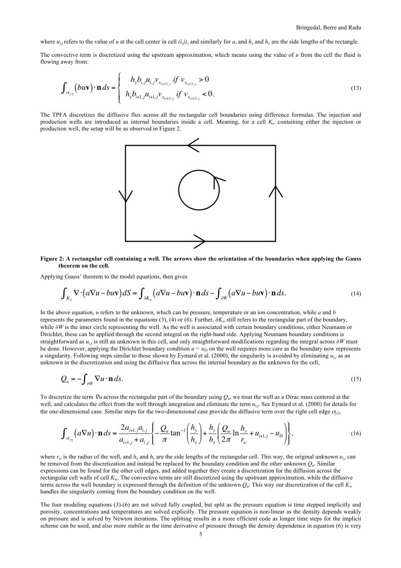
The TPFA discretizes the diffusive flux across all the rectangular cell boundaries using difference formulas. The injection and production wells are introduced as internal boundaries inside a cell. Meaning, for a cell Kw containing either the injection or production well, the setup will be as observed in Figure 2.

Figure 2: A rectangular cell containing a well. The arrows show the orientation of the boundaries when applying the Gauss theorem on the cell.

Applying Gauss’ theorem to the model equations, then gives

∇⋅Kw∫ a∇u− buv( )dS = a∇u− buv( ) ⋅nds− a∇u− buv( ) ⋅nds

∂W∫∂Kw∫ . (14)

In the above equation, u refers to the unknown, which can be pressure, temperature or an ion concentration, while a and b represents the parameters found in the equations (3), (4) or (6). Further, ∂Kw still refers to the rectangular part of the boundary, while ∂W is the inner circle representing the well. As the well is associated with certain boundary conditions, either Neumann or Dirichlet, these can be applied through the second integral on the right-hand side. Applying Neumann boundary conditions is straightforward as ui,j is still an unknown in this cell, and only straightforward modifications regarding the integral across ∂W must be done. However, applying the Dirichlet boundary condition u = uD on the well requires more care as the boundary now represents a singularity. Following steps similar to those shown by Eymard et al. (2000), the singularity is avoided by eliminating ui,j as an unknown in the discretization and using the diffusive flux across the internal boundary as the unknown for the cell,

Qu = − ∇u ⋅nds∂W∫ . (15)

To discretize the term łu across the rectangular part of the boundary using Qu, we treat the well as a Dirac mass centered at the well, and calculates the effect from the well through integration and eliminate the term ui,j. See Eymard et al. (2000) for details for the one-dimensional case. Similar steps for the two-dimensional case provide the diffusive term over the right cell edge σy2,

a∇u( ) ⋅ndsσ y2∫ =

2ai+1, jai, jai+1, j + ai, j

−Qu

πtan−1

hyhx

%

&'

(

)*+

hyhx

Qu

2πln hxrw+ui+1, j −uD

%

&'

(

)*

+,-

.-

/0-

1-, (16)

where rw is the radius of the well, and hx and hy are the side lengths of the rectangular cell. This way, the original unknown ui,j can be removed from the discretization and instead be replaced by the boundary condition and the other unknown Qu. Similar expressions can be found for the other cell edges, and added together they create a discretization for the diffusion across the rectangular cell walls of cell Kw. The convective terms are still discretized using the upstream approximation, while the diffusive terms across the well boundary is expressed through the definition of the unknown Qu. This way our discretization of the cell Kw handles the singularity coming from the boundary condition on the well.

The four modeling equations (3)-(6) are not solved fully coupled, but split as the pressure equation is time stepped implicitly and porosity, concentrations and temperatures are solved explicitly. The pressure equation is non-linear as the density depends weakly on pressure and is solved by Newton iterations. The splitting results in a more efficient code as longer time steps for the implicit scheme can be used, and also more stabile as the time derivative of pressure through the density dependence in equation (6) is very

Bringedal, Berre and Radu

6

weak. Using this splitting, the pressure, which varies slowly, is updated less frequently than the other variables, which vary more abruptly. Both the implicit and explicit time step lengths are adaptive. The sequential solution approach also allows for development of tailored numerical approaches for the equations.

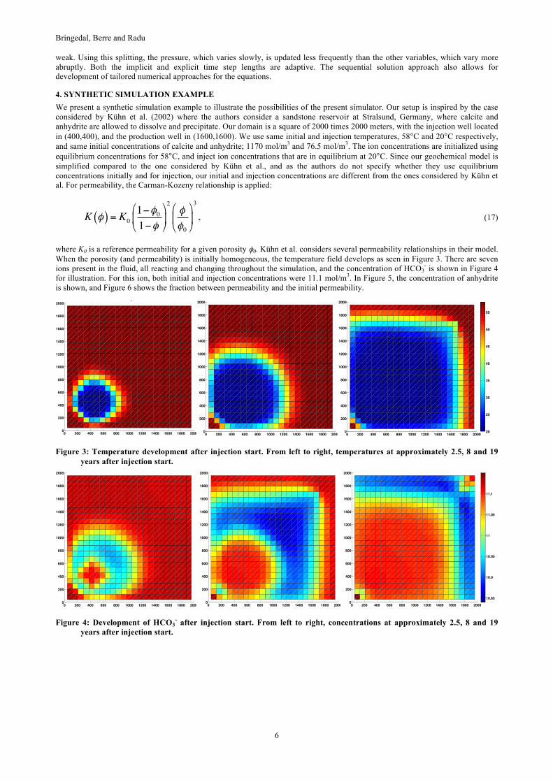
4. SYNTHETIC SIMULATION EXAMPLE We present a synthetic simulation example to illustrate the possibilities of the present simulator. Our setup is inspired by the case considered by Kühn et al. (2002) where the authors consider a sandstone reservoir at Stralsund, Germany, where calcite and anhydrite are allowed to dissolve and precipitate. Our domain is a square of 2000 times 2000 meters, with the injection well located in (400,400), and the production well in (1600,1600). We use same initial and injection temperatures, 58°C and 20°C respectively, and same initial concentrations of calcite and anhydrite; 1170 mol/m3 and 76.5 mol/m3. The ion concentrations are initialized using equilibrium concentrations for 58°C, and inject ion concentrations that are in equilibrium at 20°C. Since our geochemical model is simplified compared to the one considered by Kühn et al., and as the authors do not specify whether they use equilibrium concentrations initially and for injection, our initial and injection concentrations are different from the ones considered by Kühn et al. For permeability, the Carman-Kozeny relationship is applied:

K φ( ) = K01−φ01−φ"

#$

%

&'

2φφ0

"

#$

%

&'

3

, (17)

where K0 is a reference permeability for a given porosity φ0. Kühn et al. considers several permeability relationships in their model. When the porosity (and permeability) is initially homogeneous, the temperature field develops as seen in Figure 3. There are seven ions present in the fluid, all reacting and changing throughout the simulation, and the concentration of HCO3

- is shown in Figure 4 for illustration. For this ion, both initial and injection concentrations were 11.1 mol/m3. In Figure 5, the concentration of anhydrite is shown, and Figure 6 shows the fraction between permeability and the initial permeability.

Figure 3: Temperature development after injection start. From left to right, temperatures at approximately 2.5, 8 and 19 years after injection start.

     Figure 4: Development of HCO3

- after injection start. From left to right, concentrations at approximately 2.5, 8 and 19 years after injection start.

0 200 400 600 800 1000 1200 1400 1600 1800 20000

200

400

600

800

1000

1200

1400

1600

1800

2000 2.5793 years

20

25

30

35

40

45

50

55

0 200 400 600 800 1000 1200 1400 1600 1800 20000

200

400

600

800

1000

1200

1400

1600

1800

2000 8.1887 years

20

25

30

35

40

45

50

55

0 200 400 600 800 1000 1200 1400 1600 1800 20000

200

400

600

800

1000

1200

1400

1600

1800

2000 19.3516 years

20

25

30

35

40

45

50

55

0 200 400 600 800 1000 1200 1400 1600 1800 20000

200

400

600

800

1000

1200

1400

1600

1800

2000 2.5793 years

10.85

10.9

10.95

11

11.05

11.1

0 200 400 600 800 1000 1200 1400 1600 1800 20000

200

400

600

800

1000

1200

1400

1600

1800

2000 8.1887 years

10.85

10.9

10.95

11

11.05

11.1

0 200 400 600 800 1000 1200 1400 1600 1800 20000

200

400

600

800

1000

1200

1400

1600

1800

2000 19.3516 years

10.85

10.9

10.95

11

11.05

11.1

Bringedal, Berre and Radu

7

Figure 5: Development of CaSO4 after injection start. From left to right, concentrations at approximately 2.5, 8 and 19 years after injection start.

Figure 6: Development of permeability relative to the initial permeability after injection start. From left to right, permeabilities at approximately 2.5, 8 and 19 years after injection start.

As the injected cold fluid flows towards the production well, Figure 3 shows how the cold temperature spread out through the domain. There is a relatively large diffusivity; resulting in the temperature front being quite smooth. As all domain boundaries are no flow boundaries, the fluid flow is directed towards the production well. Both initial and injection concentration of HCO3

- is 11.1 mol/m3; hence all changes in concentrations are due to reaction (7c). We observe in Figure 4, especially in the middle figure, that reactions also take place in front of the temperature front. This is due to the wells altering the pressure in the domain, hence affecting the density of the fluid, which again affects the chemical equilibriums. There is a smooth reaction front right behind the smooth temperature front; as the temperature is changing in this region, the equilibriums of the ions are also changing, hence affecting the ion concentrations. Figure 5 shows how anhydrite is precipitated away from the well, giving an increase in the mineral concentration. Most anhydrite is precipitated along the diagonal from the injection to the production well. This effect is due to the fluid flow mainly being along this diagonal, resulting in more minerals being precipitated in this region. Small amounts of anhydrite are dissolved near the injection well giving a smaller concentration here.

The permeability is affected by the porosity, which is affected by precipitation and dissolution of both calcite and anhydrite. The development of calcite is not shown, but simulations resulted in large amounts of calcite dissolving near the injection well, but calcite was not so reactive further away from the injection well. In the figure of the permeability, there is an increase of the permeability near the injection well, which is mainly due to the dissolution of calcite, but also due to anhydrite dissolving. Further away from the injection well, the permeability is affected by anhydrite precipitating. Our findings for the permeability are in qualitative correspondence with the findings of Kühn et al. (2002): Kühn et al. found a larger increase in the permeability near the injection well as larger amounts of anhydrite dissolved in their model. This is most likely due to different choices in geochemical model and injecting different ion concentrations.

The observed changes in permeability are relatively small, only reaching a maximum increase of 1.5 % and maximum decrease of 0.5 % compared to the initial permeability. The changes in permeability are highly affected by the injected ion concentrations and injection temperature. Applying lower ion concentrations in the injected fluid, or lower injection temperature, will likely cause larger changes in the permeability, and can affect the fluid flow through the domain to a larger extent than observed in the present example.

We also consider a case with a strip of larger porosity and permeability along the diagonal from the injection to the production well. In Figure 7 we see the temperature distributions for this simulation, while in Figure 8 shows HCO3

- concentrations. Anhydrite concentrations are shown in Figure 9, while the permeability compared to initial permeability is found in Figure 10.

0 200 400 600 800 1000 1200 1400 1600 1800 20000

200

400

600

800

1000

1200

1400

1600

1800

2000 2.5793 years

75

76

77

78

79

80

81

0 200 400 600 800 1000 1200 1400 1600 1800 20000

200

400

600

800

1000

1200

1400

1600

1800

2000 8.1887 years

75

76

77

78

79

80

81

0 200 400 600 800 1000 1200 1400 1600 1800 20000

200

400

600

800

1000

1200

1400

1600

1800

2000 19.3516 years

75

76

77

78

79

80

81

0 200 400 600 800 1000 1200 1400 1600 1800 20000

200

400

600

800

1000

1200

1400

1600

1800

2000 2.5793 years

0.995

1

1.005

1.01

1.015

0 200 400 600 800 1000 1200 1400 1600 1800 20000

200

400

600

800

1000

1200

1400

1600

1800

2000 8.1887 years

0.995

1

1.005

1.01

1.015

0 200 400 600 800 1000 1200 1400 1600 1800 20000

200

400

600

800

1000

1200

1400

1600

1800

2000 19.3516 years

0.995

1

1.005

1.01

1.015

Bringedal, Berre and Radu

8

Figure 7: Temperature development after injection start. From left to right, temperatures at approximately 2.5, 8 and 19.5 years after injection start.

Figure 8: Development of HCO3- after injection start. From left to right, concentrations at approximately 2.5, 8 and 19.5

years after injection start.

Figure 9: Development of CaSO4 after injection start. From left to right, concentrations at approximately 2.5, 8 and 19.5 years after injection start.

0 200 400 600 800 1000 1200 1400 1600 1800 20000

200

400

600

800

1000

1200

1400

1600

1800

2000 2.5788 years

20

25

30

35

40

45

50

55

0 200 400 600 800 1000 1200 1400 1600 1800 20000

200

400

600

800

1000

1200

1400

1600

1800

2000 8.1235 years

20

25

30

35

40

45

50

55

0 200 400 600 800 1000 1200 1400 1600 1800 20000

200

400

600

800

1000

1200

1400

1600

1800

2000 19.7422 years

20

25

30

35

40

45

50

55

0 200 400 600 800 1000 1200 1400 1600 1800 20000

200

400

600

800

1000

1200

1400

1600

1800

2000 2.5788 years

10.85

10.9

10.95

11

11.05

11.1

11.15

0 200 400 600 800 1000 1200 1400 1600 1800 20000

200

400

600

800

1000

1200

1400

1600

1800

2000 8.1235 years

10.85

10.9

10.95

11

11.05

11.1

11.15

0 200 400 600 800 1000 1200 1400 1600 1800 20000

200

400

600

800

1000

1200

1400

1600

1800

2000 19.7422 years

10.85

10.9

10.95

11

11.05

11.1

11.15

0 200 400 600 800 1000 1200 1400 1600 1800 20000

200

400

600

800

1000

1200

1400

1600

1800

2000 2.5788 years

75

76

77

78

79

80

81

0 200 400 600 800 1000 1200 1400 1600 1800 20000

200

400

600

800

1000

1200

1400

1600

1800

2000 8.1235 years

75

76

77

78

79

80

81

0 200 400 600 800 1000 1200 1400 1600 1800 20000

200

400

600

800

1000

1200

1400

1600

1800

2000 19.7422 years

75

76

77

78

79

80

81

0 200 400 600 800 1000 1200 1400 1600 1800 20000

200

400

600

800

1000

1200

1400

1600

1800

2000 2.5788 years

0.995

1

1.005

1.01

1.015

0 200 400 600 800 1000 1200 1400 1600 1800 20000

200

400

600

800

1000

1200

1400

1600

1800

2000 8.1235 years

0.995

1

1.005

1.01

1.015

0 200 400 600 800 1000 1200 1400 1600 1800 20000

200

400

600

800

1000

1200

1400

1600

1800

2000 19.7422 years

0.995

1

1.005

1.01

1.015

Bringedal, Berre and Radu

9

Figure 10: Development of permeability relative to the initial permeability after injection start. From left to right, permeabilities at approximately 2.5, 8 and 19.5 years after injection start.

From the plots of the temperature profiles, the temperature front is more drop-shaped due to the larger permeability along the diagonal. As earlier there is not a sharp interface due to large diffusivity, and in this case the colder temperatures reach the production well faster due to the larger permeability along the diagonal. Also for the concentration of HCO3

-, Figure 8 shows a drop-shaped evolution for the injected ions as the fluid flow is mainly along the diagonal. As before there are chemical reaction occurring in the region closer to the production well due to changes in pressure. The development of anhydrite in Figure 9 is similar to the one observed in the previous case, but we can also see the effect from the larger permeability along the diagonal here, especially in the two last figures: As the main part of fluid flow is along the diagonal, most of the mineral precipitation has occurred here, and the larger amounts of anhydrite located along the diagonal is clearly seen in the rightmost plot of Figure 9. Also for the permeability seen in Figure 10, the different initial permeability has affected the end permeability. Since the fluid flow has been largest along the diagonal, mineral has dissolved and precipitated more along the diagonal compared to the previous case.

At the outermost region of where the permeability has decreased, there is a distinct stronger decrease of the permeability, as seen particularly in the rightmost plot in Figure 10. The corresponding plots in Figure 9 indicate that this stronger decrease in permeability is caused by more anhydrite precipitating in this region. Comparing with the temperature distribution in Figure 7, the region of stronger permeability decrease corresponds to the region of the smoothed temperature front. In this region the temperature is still affected by cooling, while ions are less mobile due to smaller flow velocities, forcing more anhydrite to precipitate.

5. DISCUSSION AND FURTHER WORK We have presented a mathematical model and numerical approach to describe the effect of changing porosity in a geothermal reservoir. The model equations are highly coupled and demanding to solve, and we propose a mass conservative finite volume approach to discretize the model equations. Our synthetic example illustrates coupled geochemical rock-fluid interactions. The mathematical model and numerical approach represents our initial attempt towards investigating porosity effects in a geothermal reservoir. The presented model is simplified as only a few ions are considered instead of a more complete geochemical model. Also, effects from pore size distribution, which is believed to have an impact on the permeability (Bear, 1972; Emmanuel and Ague, 2009), have been neglected. The approach we have suggested is suitable as a starting point for further development of mathematical models and tailored numerical schemes for handling the leading, coupled physical effects. In the future, we plan to expand the geochemical model to investigate additional chemical effects relevant for causing permeability changes. Also, we wish to perform a homogenization study for a pore scale model to achieve expressions for both reaction rates and permeability that depend on pore scale effects. A similar homogenization for upscaling pore scale models of mineral precipitation and dissolution has been performed by van Noorden (2009) and Kumar et al. (2011), but without the temperature dependency. We also aim at including our findings in the Matlab Reservoir Simulation Toolbox (MRST) (Lie et al., 2012), which allows for complex reservoir simulations including fractures (Sandve et al., 2012) based on finite volume discretizations on unstructured grids. Then, geochemical effects can be investigated by use of a framework that provides simulations for unstructured fractured porous media, which are relevant for geothermal applications.

ACKNOWLEDGEMENTS This work has been partly funded by the Research Council of Norway, grant number 228832.

REFERENCES Bear, J.: Dynamics of Fluids in Porous Media, American Elsevier Publishing Company, New York, (1972).

Bartels, J., Clauser, C., Kühn, M., Pape, H., and Schneider, W.: Reactive Flow and Permeability Prediction – Numerical Simulation of Complex Hydrogeothermal Problems, Petrophysical Properties of Crystalline Rocks, 24, (2005), 133-151.

Bundschuh, J., and Zilberbrand, M.: Geochemical Modeling of Groundwater, Vadose and Geothermal Systems, CRC Press (2011).

Chen, J., and Liu, C.: Numerical Simulation of the Evolution of Aquifer Porosity and Species Concentrations during Reactive Transport, Computers & Geosciences, 28, (2002), 485-499.

Cheng, H., and Yeh, G.: Development and Demonstrative Application of a 3-D Numerical Model of Subsurface Flow, Heat Trasnfer, and Reactive Chemical Transport: 3HYDROGEOCHEM, Journal of Contaminant Hydrology, 34, (1998), 47-83.

Clauser, C.: Numerical Simulation of Reactive Flow in Hot Aquifers: SHEMAT and Processing SHEMAT, Springer, (2003).

Emmanuel, S., and Ague, J.J.: Modeling the Impact of Nano-Pores on Mineralization in Sedimentary Rocks, Water Resources Research, 45, (2009).

Eymard, R., Gallouët, T., and Herbin, R.: Finite Volume Methods, Handbook of numerical analysis, 7, (2000), 713-1018.

Kühn, M., Bartels, J., and Iffland, J.: Predicting Reservoir Property Trends under Heat Exploitation: Interaction between Flow, Heat Transfer, Transport and Chemical Reaction in a Deep Aquifer at Stralsund, Germany, Geothermics, 31, (2002), 725-749.

Kumar, K., van Noorden, T.L., and Pop, I.S.: Effective Dispersion Equations for Reactive Flows Involving Free Boundaries at the Microscale, Multiscale Modeling & Simulation, 9, (2011), 29-58.

Lie, K.A., Krogstad, S., Ligaarden, I.S., Natvig, J.R., Nilsen, H.M., and Skaflestad, B.: Open Source MATLAB Implementation of Consistent Discretisations on Complex Grids, Comput. Geosci., Vol. 16, No. 2, (2012), 297-322.

McLin, K.S., Kovac, K.M., Moore, J.N., Adams, M.C., and Xu, T.: Modeling the Geochemical Effects of Injection at Coso Geothermal Field, CA; Comparion with Field Obersvations, Proceedings, Thirty-first Workshop on Geothermal Reservoir Engineering, Stanford University, Stanford, CA (2006).

Bringedal, Berre and Radu

10

Moore, D.E., Morrow, C.A., and Byerlee, J.D.: Chemical Reactions Accompanying Fluid Flow through Granite Held in a Temperature Gradient, Geochimica et Cosmochimica Acta, 47, (1983), 445-453.

Mroczek, E.K., White, S.P., and Graham, D.J.: Deposition of Amorphous Silica in Porous Packed Beds – Predicting the Lifetime of Reinjection Aquifers, Geothermics, 29, (2000), 737-757.

Pape, H, Clauser, C., Iffland, J., Krug, R., and Wagner, R.: Anhydrite Cementation and Compaction in Geothermal Reservoirs: Interaction of Pore-space Structure with Flow, Transport, P-T Conditions, and Chemical Reactions, International Journal of Rock Mechanics & Mining Sciences, 42, (2005), 1056-1069.

Plummer, L.N., Parkhurst, D.L., Fleming, G.W., and Dunkle, S.A.: A Computer Program Incorporating Pitzer’s Equations for Calculation of Geochemical Reactions in Brines, Department of the Interior, US Geological Survey (1988).

Portier, S., Vuataz, F.D., Martinez, A.L.B., and Siddiqi, G.: Preliminary Modelling of the Permeability Reduction in the Injection Zone at Berlin Geothermal Field, El Salvador, Proceedings, World Geothermal Congress, session 22, 2231, 1-7, (2010).

Sandve, T.H., Berre, I., and Nordbotten, J.M.: An Efficient Multi-Point Flux Approximation Method for Discrete Fracture-Matrix simulations, Journal of Computational Physics, 231, (2012), 3784-3800.

Sonnenthal, E., Ito, A., Spycher, N., Yui, M., Apps, J., Sugita, Y., Conrad, M., and Kawakami, S.: Approaches to Modeling Coupled Thermal, Hydrological, and Chemical Processes in the Drift Scale Heater Test at Yucca Mountain, International Journal of Rock Mechanics & Mining Sciences, 42, (2005), 698-719.

Steefel, C.I., and Lasaga, A.C.: A Coupled Model for Transport of Multiple Chemical Species and Kinetic Precipitation/Dissolution Reactions with Application to Reactive Flow in Single Phase Hydrothermal Systems, American Journal of Science, 5, (1994), 529-592.

Taron, J., and Elsworth, D.: Thermal-Hydrologic-Mechanical-Chemical Processes in the Evolution of Engineered Geothermal Reservoirs, International Journal of Rock Mechanics & Mining Sciences, 46, (2009), 855-864.

van Noorden, T.L.: Crystal Precipitation and Dissolution in a Porous Medium: Effective Equations and Numerical Experiments, Multiscale Modeling & Simulation, 7, (2009), 1220-1236.

Wagner, R., Kühn, M., Meyn, V., Pape, H., Vath, U., and Clauser, C.: Numerical Simulation of Pore Space Clogging in Geothermal Reservoirs by Precipitation of Anhydrite, International Journal of Rock Mechanics & Mining Sciences, 42, (2005), 1070-1081.

Wells, J.T., and Ghiorso, M.S.: Coupled Fluid Flow and Reaction in Mid-Ocean Ridge Hydrothermal Systems: The Behaviour of Silica, Geochimica et Cosmochimica Acta, 55, (1991), 2467-2481.

White, S.P., and Mroczek, E.K.: Permeability Changes During the Evolution of a Geothermal Field Due to the Dissolution and Precipitation of Quartz, Transport in Porous Media, 33, (1998), 81-101.

Xu, T., and Preuss, K.: Coupled Modeling of Non-Isothermal Multiphase Flow, Solute Transport and Reactive Chemistry in Porous and Fractured Media: 1. Model Development and Validation, Lawrence Berkeley National Laboratory Report LBNL-42050, Berkeley, California, 38 pp., 1998.