202.? 92AP Infrastructure and Urban Development Department The World Bank October 1992 WPS 1005 An Approach to the Economic Analysis of Water Supply Projects Laszlo Lovei A simplified method aimed at improving the quality of economic analysis on water supply projects. Policy Research Woiking Papers disseminate the findings of work in progress and encourage the exchange of ideas among B ank staff and all others interested in developmcni issues. These papers carry ihc names of the authois, reflect only their views, and should be used and cited accordingly. The findings, interpretations, and conclusions are the authors' own. They should not be attributed I its Board of Directors, its management, or any of its member countries. o ~7 C\ <? A o I "7 iLO L' f- — Ji fiy I I 2S 7 1
Transcript
202.? 92AP
Infrastructure and Urban DevelopmentDepartment
The World BankOctober 1992
WPS 1005
An Approachto the Economic Analysisof Water Supply Projects
Laszlo Lovei
A simplified method aimed at improving the quality of economicanalysis on water supply projects.
Policy Research Woiking Papers disseminate the findings of work in progress and encourage the exchange of ideas among B ank staff andall others interested in developmcni issues. These papers carry ihc names of the authois, reflect only their views, and should be used andcited accordingly. The findings, interpretations, and conclusions are the authors' own. They should not be attributed Iits Board of Directors, its management, or any of its member countries. o ~7 C\ <? A o I "7
iLO L' f- — Ji fiy I I 2S 7 1
WPS 1005
This paper— a product of the Infrastructure, Energy, and Environment Division, Europe and Central AsiaCountry Department III — is part of a larger effort in the Bank to improve operational practice and raisethe quality of projects in the water and sanitation sector. Copies of the paper are available free from theWorld Bank, 1818 H Street NW, Washington DC 20433. Please contact Man Dhokai, room S12-005,extension 33970 (October 1992, 37 pages).
Development economists are increasinglyconcerned about the correct approach to eco-nomic analysis of projects. By looking for acompromise between theory (which identifiesideals) and practice (which deals within thebounds of time and resource constraints), Loveifocuses on potential guidelines for economicappraisals of water supply projects.
He summarizes theory and the current WorldBank guidelines on the economic analysis of
water supply projects; reviews the method ofeconomic analysis applied in 21 recently ap-proved Bank projects; and describes a simplifiedmethod that was tested in practice and found toimprove substantially the quality of economicanalysis in the sector.
This new method relies on standardized andrigorous use of information that is routinelyavailable during the preparation of water supplyprojects.
The Policy Research Working Paper Series disseminates the findings of work under way in the B ank. An objective of the seriesis to get these findings out quickly, even if presentations are less than fully polished. The findings, interpretations, andconclusions in these papers do not necessarily represent official Bank policy.
Produced by the Policy Research Dissemination Center
An Approach to the Economic Analysisof Water Supply Projects
by
Laszlo Lovei
Laszlo Lovei is an economist in the Infrastructure, Energy and Environment Divisionof Country Department EC3 of the World Bank. The author would like to thank IanBartlett, Colin Gannon, Christian Gomez, Luis Gutierrez, Lars Jeurling, Mike Gam,Chris Shugart, and Dale Whittington for their comments on earlier versions of thepaper and the ECOWAT programs.
Table of Contents
1. Summary 3
2. Theory and Guidelines 3
3. Current Practice at the World Bank 4
4. A Proposal for Improvement 7
References 14
Annex 1: Staff Appraisal Reports Reviewed 15
Annex 2: Numerical Example 16
Annex 3: Introduction to EC0WAT1 17Mathematical Formulas of ECO WATl ; 25
Annex 4: Introduction to EC0WAT2 28
1. Summary
Development economists in the World Bank andelsewhere are increasingly concerned about the correctapproach to economic analyses of projects.1 By lookingfor a compromise between theory (which identifies ideals)and practice (which deals within the bounds of time andresource constraints), this paper focuses on potentialguidelines for project economic appraisal in the watersupply sector. No "finalsolution" is proposed here, but thediscussion should stimulate further efforts to develop aresponsive approach.
The first section of the paper summarizes thetheory and the current World Bank guidelines on theeconomic analysis of water supply projects. The nextsection reviews the method of economic analysis appliedin 21 recently approved Bank projects, and the finalsection describes a simplified method that was tested inpractice and found to improve substantially the quality ofeconomic analysis in the sector. This method relies onstandardized and rigorous use of information that isroutinely available during the preparation of watersupplyprojects.
2. Theory and Guidelines
, Water is a good that has both consumption valueand, in certain circumstances, value from external ben-efits for those who do not consume it. In theory, thebenefits of private goods are fully divisible and exclud-able, and the benefits of public goods are indivisible andnonexcludable.2 Industrial water is a private good, butresidential water can supply external health benefits andis therefore neither a purely private nor public good. On
the spectrum of private to public goods, residential waterlies between the two extremes, probably closer to pureprivate goods.
The economic analysis (or cost-benefit analysis;these terms are used interchangeably in this paper) ofwater supply projects consists of the (1) estimation ofproject costs; (2) estimation of project benefits; and (3)comparison of costs and benefits (over time, with uncer-tainty). While project costs are estimated in the same wayfor water supply as for other sectors, estimating thebenefits, particularly for a residential water supply com-ponent, is not so straightforward. For example, estimatingbenefits by using a measure of consumer willingness topay captures only private gains and does not account forthe public health improvements in the community at large.Public benefits are generally considered difficult to quan-tify and intangible.3 Moreover, willingness to pay pro-vides a good estimate of project benefits only whenconsumers fully understand the relationship between waterand their own health.
In economic analysis, both costs and benefits aredefined as the difference between results with the projectand without it. The analyst develops these two scenariosin sufficient detail to estimate the difference for the periodof project implementation and operation.
1 See, for example, Little and Mirrlees (1990), Anderson(1989).2 For a useful definition of these terms, see Comes andSandier (1986).
3 For a brief review of the literature on the quantificationof health benefits, see Churchill (1987) pp. 10-12. In fact,although it requires voluminous data, it is possible toassess the monetary scale of health effects, as demon-strated in Harrington, Krupnick, and Spofford (1989).That paper analyzes the effects of an outbreak of waterbornedisease and estimates nine categories of economic losses:doctor visits, hospital visits, emergency room visits, tests,medication, time and travel losses associated with medi-cal treatment, work loss, work productivity loss, andleisure time loss.
World Bank guidelines on economic analysis donot separately discuss water supply projects.4 The guide-lines present a general description of cost-benefit analysisbut not a blueprint for the sector practitioner. Variouscentral concepts are briefly addressed, such as "with" and"without" scenarios, willingness to pay, external benefits,non-quantification of benefits. Yet there is no guidance onhow to estimate consumer willingness to pay. However,detailed entries cover other problems, such as the selec-tion of a numeraire, valuation of traded and nontradedgoods, conversion factors, shadow wage, and interestrates.
Operational Manual Statement (OMS) 3.72 onthe preparation of "Energy, Water Supply and Sanitation,and Telecommunications" (EWT) projects contains sixparagraphs on the subject of "economic justification."Three steps are mentioned: (1) estimation of demand; (2)selection of the least cost supply option; (3) comparison ofcosts and benefits. However, the last step is consideredquite difficult5 in practice; therefore, the calculation of thefinancial internal rate of return (FTRR; adjusted for trans-fer payments) is proposed since it "usually represents atleast a minimum estimate of the economic rate of return."There is no guidance on the procedures to be followed ifthe financial rate of return is below the opportunity cost ofcapital.*
3. Current Practice at the WorldBank
To assess the existing Bank practice, Staff Ap-praisal Reports (SAR) of 21 recently approved watersupply projects were reviewed.7 Four different approachesto economic analysis can be identified. One SAR demon-strated that the project was the least-cost solution to meetassumed demand but did not go further. Let's call this atype A analysis. Fourteen SARs calculated the financialinternal rate of return of the project and briefly mentionedother, non-quantified benefits. That is type B analysis.
"See World Bank Operational Manual Statement 2.21.5 Operational Manual Statement 3.72, para. 34 states, "Inmost cases it will not be possible to quantify the economicbenefits by consumers in excess of amounts they actuallypay, and therefore the estimation of the social value of theproject is precluded."6 "A low return may simply indicate that tariffs are too low,rather than that the project is not justified." OMS 3.72,para. 34.7 For a list of the SARs reviewed, see Annex 1.
Three SARs calculated the FIRR and also provided anestimate for the consumer surplus-type C analysis. Onlythree SARs attempted to carry out an independent eco-nomic analysis without relying on the projected financialrevenue stream—type D analysis.
Generally, type A analysis is justified when themajority of project benefits are considered non-quantifi-able and the benefits of different supply options arethought to be the same. In practice, there are two problemswith this approach. First, while the relative importance ofexpected health benefits may change from one watersupply project to another, non-health-related benefits areseldom negligible and should be accounted for. Second, incases where benefits are intangible but quantifiable, costeffectiveness analysis is more appropriate to determinethe correct level of supply to achieve health improve-ments. Such analysis should consider whether the incre-mental health benefit due to the last unit of water suppliedmight be achievable at lower cost.
Type A, or least-cost analysis, has to be per-formed during the preparation of any water supply project,for example, to select the best water source.8 It shouldcome before the calculation of project costs. However, ifthe analyst only wants to ensure the economic viability ofthe project and is not interested in the net present value orthe economic rate of return, then, assuming certain condi-tions are met, the estimation of benefits can be consideredunnecessary. If the average incremental cost (AIC) ofwater* is equal to or less than the water tariff, and thedemand at that tariff is estimated with reasonable cer-tainty, it can be said without further analysis that theeconomic rate of return of the project is not less than theopportunity cost of capital. However, not all waterprojectsin developing countries meet these conditions. In the caseof the SAR that simply conducted a least-cost analysis,10
the existing tariff was only 70 percent of the AIC and eventhe projected tariff (six years later) was less than the AIC.
8 See OMS 3.72, para. 32.9 AIC is defined as C/Q, where C and Q are the discountedpresent value of incremental costs and incremental waterquantity supplied, respectively. The discount rate is equalto the opportunity cost of capital, and incremental meansthe difference between the "with" and "without" projectscenarios.10 As a matter of fact, the SAR presented an economic rateof return calculation based on the com parison between theleast cost and the second least-cost solution to the problemof providing the water source for the piped supply system.There was no comparison with the "without" projectscenario.
Type B analysis has two potential problems. Thefirst and more important problem is the reliability of theestimated incremental revenue stream. Water demand isa function of the price of water. Therefore the standardprocedure of estimating water sales independently andmultiplying that with the projected tariff is highly ques-tionable (unless the price elasticity of water demand isvery low over the whole range of relevant supply levels).The larger projected tariff increases are, the less reliableare the revenue estimates. None of the type B analysesexamined the relationship between water tariff and waterconsumption. If no tariff increase was expected, this mightbe acceptable. But in 5 out of the 14 cases tariff increasesranging from 40 to 300 percent (in real terms) werecalculated into the estimates of incremental revenues.
The second problem is the usefulness of theestimated FIRR. If the tariff is expected to stay at thepresent level and the estimated FIRR is higher than theopportunity cost of capital, the project is justified.11
Among the nine type B analyses that did not project a tariffincrease, only three estimated the FIRR to be higher thanthe opportunity cost of capital (assuming a 10 percent ratefor the sake of simplicity). For additional justification, theother six type B analyses referred to non-quantifiedbenefits.12 However, it is not possible to assess whether, ifquantified, those benefits would have made the projectseconomically viable. In these cases, without additionalinformation, the FIRR calculations did not give enoughsupport to decision making and only indicated how highthe non-quantified benefits need to be.
The three type C analyses tried to come up withthe additional information by estimating the value ofconsumer surplus. To do that, the water demand functionhad to be estimated in the relevant range. The sameprocedure was followed in all three cases: the coordinatesof two points on the ordinary (uncompensated) demand
11 See OMS 3.72, para. 34.12 One SAR, without presenting a demand analysis, usedthe assumed tariff as a proxy for benefits of proposed smallrural water supply schemes. The tariff was simply set toachieve the required level of cost recovery (part of thecapital cost and all operation and maintenance costs)."Additional" benefits were mentioned without quantifi-cation: time savings because water would be carried overshorter distances, fuel cost savings because less boilingwould be required, and health benefits. Since these ben-efits are usually the reason why consumers might bewilling to pay for water, quantifying them would lead todouble counting.
function" were determined and then connected by a linearor loglinear curve. After the demand curve and quantitiesconsumed under the "with" and "without" scenarios hadbeen estimated, the calculation of the area that representedconsumer surplus was relatively straightforward.
Accuracy of the whole procedure depends on theselection of the two points on the demand curve. That isexactly where two of the analyses went wrong. Coordi-nates of the first point were based on the price and quantityof water purchased by households from distributing ven-dors. Projected piped water consumption and water tariffdetermined the coordinates of the second point. But thesetwo points are not on the same demand curve. Connectedhouseholds use piped water for drinking, cooking, bath-ing, washing, and sometimes even for gardening. Watersold by distributing vendors is used only for drinking andcooking (sometimes for bathing). This is reflected in thesmall quantities purchased, 5-20 liters per capita per day(1/c/d). Bathing, washing, and other water demand isusually met from secondary sources like shallow wells,rivers, and ponds that provide lower quality water at lowercost. When there is no information on water purchasedfrom vendors, other than the price and quantity, consis-tency requires that the other point on the demand curve bebased on piped water consumption for drinking/cookingonly.
The third type C analysis tried to place bothpoints on the same demand curve by restricting thecalculation of consumer surplus to the first 15 1/c/d ofpiped water.14 However, that may actually have underes-timated the benefits of piped water supply. When pipedwater costs less than other nonpiped sources, consumerswill enjoy a surplus on their water for other use also.Despite this discrepancy, such a conservative approachmight be useful when the FIRR (based on existing tariff)is close to the opportunity cost of capital.
If a second point on the demand curve representsthe full quantity of piped water consumption, the first
13 For the definition of ordinary and compensated demandfunctions and a review of the relationship between ordi-nary demand functions, consumer surplus, and compen-sating variation, see Johansson (1987) Chapter 4.14 While the method of estimating part of the consumersurplus appears correct, estimates of water sales revenueand the economic rate of return (ERR, in this case 11percent) are questionable. The revenue stream was basedon a tariff increase of more than 500 percent (in real terms)during the first six years of the project, apparently with noeffect on water consumption.
point must be based on observations of water use from allavailable sources. Otherwise, as in two of the type Canalyses, consumer surplus can be grossly overestimated.Both analyses aimed to determine only the average valueof consumer surplus based on cubic meters of waterconsumed. To do that, each calculated the area of thetriangle under the demand curve between the quantity soldby vendors and the quantity provided by the piped watersystem and therefore implicitly assumed that the "withoutproject" consumption was not more than the amount ofwater purchased from vendors. As a result, the twoanalyses arrived at similar conclusions: the average valueof consumer surplus is about equal to the water tariff;therefore, total benefits should approximate two times thesales revenue.15
One of the three type D analyses provided anestimate of the average cost of existing nonpiped water(including the value of time spent fetching water) andassumed that project benefits were equal to that cost,based on cubic meters of water consumed. This procedureis correct as long as the incremental piped water deliveredby the project only replaces water from other sourceswithout resulting in an increase in overall consumption.16
However, since piped water consumption (per consumer)was projected to be higher than existing water use, andsince consumers generally assign a decreasing value toadditional water, the end result (13 percent ERR) probablyoverestimated the true economic rate of return.
While the second type D analysis initially fol-lowed a similar procedure, it recognized that additionalsupplies had a diminishing value. Although the relation-ship between water price and quantity was not describedexplicitly, it was assumed that the average value ofadditional water consumed was halfway between the priceof piped water and the current cost of nonpiped water. Thisassumption implies a demand curve that is linear betweenthe points representing existing and projected water costs
15 One of the two analyses did not stop here. "Additional"benefits were quantified, such as sickness cost avoided,fire prevention and land value increase. Beginning with anFIRR of 15 percent based on existing tariff (which meansthat the project, as a result of a type B analysis, appearsjustified), the analysis ended with an ERR of 34 percent.However, it was admitted that "some (sic) overlap mayexist between the fire and health benefits and consumersurplus."16 To be exact, two additional assumptions are needed. Itmust be assumed that there are no transfer paymentsamong the costs of existing water supply and that there isno producer surplus.
and prices. Several water supply schemes were analyzedthat way in the SAR. The calculated ERRs were between5-27 percent. There was not any cut-off level applied, andall schemes were accepted, based on additional,nonspecified, "unquantifiable" health benefits.
The third type D analysis divided the consumersinto two groups, existing consumers (already served bythe water system) and new consumers. Water demandcurves were estimated separately for each group. At firsttwo points on each demand curve were identified. Onepoint was based on drinking/cooking water demand,priced at the rate charged by water vendors, while the otherpoint was based on projected per capita piped water use,priced at the expected average tariff under the project.Again, unless vendors were the only water source used bythe nonconnected consumers, these two points are not onthe same demand curve. This might explain why the twopoints identified that way produced a (constant) priceelasticity of water demand higher than unity (in absolutevalue). To stay consistent with expectations, a variableelasticity approach was selected and the demand curvewas assumed to consist of two straight lines runningthrough the two identified points, with elasticities of (-0.2)and (-0.8).
After estimating the demand curves, the averagewillingness to pay per gallon of incremental water wasestimated for each group of consumers. Existing consum-ers' average willingness to pay was estimated at themidpoint on the demand curve between the with- andwithout-project consumption levels. One part of the waterdelivered to new consumers was assumed to replacedrinking/cooking water purchased from vendors and wasvalued at the vendor price to account for cost savings. Theother part was assumed to represent incremental con-sumption and was valued according to the demand curve.As a result, new consumers' average willingness to pay,as a proxy for project benefits, was estimated 70 percenthigher than the projected tariff. If these consumers hadbeen using other water sources in addition to vendors, thenthe applied method overestimated project benefits. How-ever, since the project's ERR was estimated at 15 percent,and less than 20 percent of incremental water would go tonew consumers, this project seems to be viable.
Altogether, only three type B and one type Danalyses appear methodologically correct out of the 21reviewed (see Table 1). That does not mean that the other17 projects are not economically viable. Some of themcould be justified on the basis of information in the SARs,but many of them cannot be assessed without furtherinformation and analysis. However, rather than assessingthe viability of these projects, this review aims to
demonstrate that currently used approaches to the eco-nomic analysis of water supply projects need substantialimprovement.
Similar conclusions appear in a number of an-nual reviews prepared by the sector policy and researchstaff of the World Bank. According to the 1990 watersector review, "the economic analysis of projects does notfollow a consistent approach and the reported rates ofreturn seem, in several cases, to be subject to substantialupward bias due either to the approach used or the dataemployed in its calculation."17 The same review observedthat, "water demand continues to be projected as a com-pletely inelastic consumption trend with an assumedgrowth in per connection consumption, unrelated to pricesassumed in financial forecasts and in revenue projectionsused in the economic justification." Obviously, specificguidelines on the economic analysis of water supplyprojects are needed to rectify these problems. The guide-lines should be based on a methodology that is flexible andstructured according to the complexity of the projects tobe analyzed-namely, it should be kept simple and thecritical assumptions of any particular case applicationshould be clear and well understood. Furthermore, themethodology should be user friendly and usable also toborrowers.
17 World Bank (1990) pp. 14-15.
4. A Proposal for Improvement
"Time for a change" -that is the subtitle of aWorld Bank discussion paper on rural water supply andsanitation issued in 1987.1' Although primarily policyoriented, the paper addresses many of the problems de-scribed here. Regarding health effects, it argues that "theexistence of substantial, health-related externalities is indoubt, given the evidence."1* On this basis, the paperrecommends that analysts should concentrate on theassessment of economic benefits of watersupply projects,especially on time savings. However, not relying onexternal health benefits to justify a project does not meanthat all health benefits are unaccountable. Health benefitsknown to users are reflected in their willingness to pay forgood quality water, and willingness to pay can be derivedfrom the demand function. This leaves only two kinds ofbenefits that cannot be captured: (1) those unknown tousers and (2) benefits to others through reduced diseasetransmission. Experience suggests that health benefitswill not materialize unless consumers understand therelationship between water and health and use waterproperly.20 Also, the people most affected by diseasetransmission are those living in the same household andprobably their benefits are reflected in consumers' will-ingness to pay.
18 Churchill (1987).19 ibid. p. 32.20 ibid. pp. 10-11.
Tablel Review of Twenty-One SARs
Problems in the AnalysisAIC > tariffTariff has no effect on demandHRR < 10%Misspecified "without project"Constant marginal utility of water
Subtotal
Correct AnalysisTotal
A(least Cost)
1
1
01
Type of Economic Analysis
BFIRR
56
11
3
14
C(FIRR+CS)
1
2
3
0
3
D(true econ. analysis)
112
13
Another World Bankpaper on rural water supplyrecommends that "for project preparation, more precisetools are needed to determine the willingness to pay fordifferent service levels and to assess the consequences ofthis information on technology choices and financialdecisions.'™ The paper identifies direct and indirect meth-ods of determining what water supply service people wantand are willing to pay for. The direct method is tointerview potential customers and ask how much they arewilling to pay for different types and levels of service.Detailed guidelines for applying this approach, called the"contingent valuation method," have been published byUSAID.22 The indirect method is to collect data on ob-served behavior (quantities of water used from differentsources, time spent collecting water, money spent onpurchasing water) and, on the basis of consumer demandtheory, infer how m uch consumers would be willing to payfor improved water supply.
The type C and type D analyses obviously triedto follow the indirect method but, at least in some aspects,applied the theory of consumer demand inconsistently.Yet, for the indirect method, all elements for practicalimprovements are readily available. Improved economicanalysis would result in better design and selection ofprojects and would potentially increase the reliability ofrevenue projections.
All the economic analyses reviewed here madethe assumption that the number of consumers connectedto the system or relying on public taps is a given. However,whether to connect to the system and how much toconsume are two interdependent decisions. Whittington,Briscoe, and Mu (1987) present a theoretical frameworkthat makes it possible to model both simultaneously. Thispaper does not deal with water source selection despite itsimportance for the economic and financial viability ofwater supply projects. The methods described here as-sume that the number of customers is known. The esti-mated demand function depends on the number of con-sumers who select water from the piped system. There-
» fore, estimated project benefits indicate potential benefitsonly. While the proposed project may appear viable, if theconsumers decide to stay with their existing sources ofwater (because of high connection charges or water tariff,or simply as a matter of taste), that potential will notmaterialize. Although estimating the number of custom-ers should be integral to any economic analysis, theproposed methodology does not cover it.
Shortcut method. This method assumes that thepurpose of economic analysis is strictly to decide whethera particular project is economically viable—namely,whether the present value of net benefits is likely to bepositive. While this approach provides a lower bound torthe expected economic benefits, it does not provide thepractitioner with an estimate of total benefits. This helpskeep the analysis simple. If an order of priority has to beassigned to a set of possible projects, the shortcut methodcannot be applied. But, since Bank appraisals usuallywork with a yes orno investment criterion (which assumesthat the opportunity cost of capital is known), it seemsworthwhile to consider the simplified approach first.
If the existing tariff is adequate to meet financingrequirements and a real tariff increase is not expected, aFIRR calculation based on existing tariff and projecteddemand can be carried out. The demand estimate shouldnot be a simple extrapolation of past trends but should takeinto account the changing composition of customers(either due to service area extension or real incomeincrease over time). If the needed information is availableor accessible, an analysis of income and water demandshould be carried out to understand better how a shifttowards higher or lower income customers will affectwater consumption. Even if there is not enough data tocompare income and water consumption, the incomeelasticity of water demand should be taken into accountwhen customers' real income is expected to rise substan-tially. An educated guess in the range of 0.4 to 0.8 (wateris a necessity) may be acceptable. Generally ERR > FIRR,therefore the project is justified if the FIRR is not less thanthe opportunity cost of capital.23 Looking at the 21 re-viewed SARs, four projects (three type B and one type C)would probably pass this test.24
If a real tariff increase is expected, projection ofwater demand requires estimation of the price effect.Since econometric investigations are data intensive andtime consuming, an educated guess is again probably the
21 Briscoe and de Ferranti (1988) p. 25.22 Whittington, Briscoe, and Mu (1987); Whittington(1988).
23 It is assumed that (1) economic costs of the project arenot higher than financial costs; (2) the project has nonegative externalities. When these conditions are not met(e.g., the planned extraction of surface or groundwater forthe piped system will decrease the availability of water forcertain consumers who will not be connected to the systemand rely on the same water sources as the project), the coststream has to be corrected before the internal rate of returncalculations are carried out.24 This test is exactly the same as described in OMS 3.72(although OMS 3.72 does not list the necessary conditionsfor the validity of the test).
most efficient way to determine the price elasticity ofwater demand. Based on econometric studies, the short-and medium-run price elasticity of water demand isusually in the -0.2 to -0.8 range.25 Price elasticity changesas one moves along the demand curve. Arc elasticity overthe assumed range of price change is more relevant foreconomic analysis than point elasticity. If known, theeffects of previous tariff increases can be analyzed toselect a particular value for the price elasticity.* After theprice effect is taken into account, the same test as abovecan be carried out to see whether the project is justified.
These demand projections assume that the ob-served quantity of piped water consumption with thecorresponding price provides a point on the demand curve.If supply is intermittent or consumption is not meteredanda flat monthly fee is charged, that assumption will beunfounded. Also, if the number of existing customers issmall compared to the planned expansion, extrapolationof observed piped water consumption patterns is highlyuncertain.
When the FIRR is below the opportunity cost ofcapital, the "shortcut" method cannot be applied. Addingconsumer surplus to the revenues might raise the calcu-lated internal rate of return; however, the consumersurplus of new customers cannot be estimated withouttaking into account their existing, nonpiped water con-sumption.21 The indirect method described below can beapplied in all these cases as well as when a completely newsystem is to be constructed.
Indirect method. Resi-dential consumers use water fordrinking, cooking, bathing, wash-ing, and so forth. The water qual-ity required depends on the pur-pose or use. Brackish water m igh tbe acceptable for washing but notfordrinking. When piped water isnot available, people usually relyon a variety of water sources:vendors, wells, rivers, ponds,springs, rainwater. Both the qual-ity and the price of water fromthese sources are different, andeach water source serves differ-ent needs. When piped water be-comes available, it is a potentialsubstitute for water from all other
project can be divided into two parts: one part replaces theprevious sources and quantity of water use, the other partis a net increase in water consumption. In this context,benefit of the first part is equal to the savings of economiccosts of consumers who do not need to use the formerwater sources any longer (the area represented by OQ ID 1P1in Graph 1). Benefit of the second part is equal to the areabelow the demand curve between the with-project andwithout-project water use of each consumer (the areaQ1Q2D2D1 in Graph 1).
Before benefits can be estimated, a survey ofexisting water consumption patterns must be undertakento determine the quantity of water used from each source
25 For example, Al-Qunaibet and Johnston (1985).26 If these effects are not documented, one could, as a lastresort, rely on Martin and Thomas (1986), who found thatthe long-run price elasticity for residential water wasabout -0.5 over a wide range of price changes and acrossseveral countries. With respect to industrial water de-mand, Renzetti (1988) found that the price elasticity wasin the -0.1 to -0.6 range, with the demand of waterintensive industries being generally more elastic.27 The without project consumption of these customerswould be zero unless nonpiped water use is also taken intoaccount.28 Whether this actually happens depends on the qualityand price of piped water compared to water from othersources.
sources.
The incremental quan-tity of piped water supplied by a
Graph 1: Benefit of Piped Water
marginalcost/price
P1
P2
D1
demandcurve
Q1 Q2
Q1 Water U M without project0 2 Water U M with traprojactP1 Marginal cosVprioa o» watar without theprojwtP2 Marginal oosVprioa of water with tfwproJMI
quantity
and the amounts spent on water sold by vendors,29 on theconstruction and repair of wells, handpumps, water stor-age tanks, and on the operation of diesel or electric pumps,and time spent collecting and carrying water and operat-ing handpumps. While the value of consumers' time is notdirectly available from the water use survey, recent re-search suggests that it is close to the market wage rate forunskilled labor.30
Unless there are indications to the contrary, it canbe assumed that actual payments represent economiccosts-that is, the production and operation of wells,storage tanks, and pumps is a competitive industry with aflat cost curve. It is also assumed that no element ofmonopolistic rent distorts the price of water sold byvendors, and that vendors who lose their jobs due to thepiped water project can find alternative occupations with-out incurring any costs.31
Usually it can be assumed that all nonpiped wateruse will be replaced by piped water in households thatchoose to connect to the piped system.32 This assumptionshould not apply to households that will be served bypublic taps; the amount of water use replaced will dependon the price of water and the location of the taps comparedto the cost and convenience of presently used watersources. After the amount and cost of replaced water areestimated, the calculation of cost savings resulting fromthe first part of water supplied by the project is relativelystraightforward (area O Q ^ P , = Qt x P,, see Graph I).33
The demand curve forpiped water is needed to estimatebenefits due to the second part. Ifthere were only one water source,the quantity and marginal cost ofwater used from the source woulddetermine a point on the pipedwater demand curve. Frequentlythere is more than one watersource used, and water from dif-ferent sources serves differentneeds. Theoretically, there is aseparate water demand curve foreach need (D W and ND in Graph2). Observations obtained from'the water use survey describe theconsumption of water from thesesources. The marginal cost ofwater from various sources is dif-ferent; therefore, the points on thedemand curves obtained from thewater use survey belong to differ-ent prices. The piped water de-
mand curve (PW) is the aggregate of these curves sincepiped water can serve all these needs. However, the pointsobtained from the survey cannot be aggregated becausetheir coordinates on the vertical axis (that is, prices P̂ and
29 When vendors are active in the project area, informationobtained from the water use survey about the cost andquantity of water purchased from vendors will be substan-tially more reliable than information describing consump-tion of water from other sources. However, water vendingis not a necessary condition for using the proposed method.30 Whittington, Mu, and Roche (1989).31 If a project is expected to replace a substantial amountof water purchased from vendors, a water-vending surveyto validate these assumptions is warranted. The surveyshould provide information about the cost and price ofwater at each phase of the vending system: at the watersource, at the retail outlets (hydrants or kiosks), and, afterdistribution, at the point of delivery to the households.32 The problem of determining how many households wantto connect to the system is not analyzed in this paper.33 Sunk costs cannot be saved, therefore only those costsshould be taken into account which would not be incurredif the project was implemented. While the cost of analready existing well or water pump cannot be avoided(that is, it is sunk except for salvage value, if any), futurereplacement costs or the cost of new wells should still beconsidered.
Graph 2: Aggregation of Water Demand Curves
price
Pd
Pnd
DWNOPWQdQndQtPdPnd
! \ !^w p w
1 I i
t" I i
Qd Qnd Qt q u a n t i t y
Drinking water demand curveNon-drinking water demand curvePiped water demand curveDrinking water oontumptionNon-drinking water oontumptionTotal water consumptionMarginal cost/price of drinking waterMarginal cost/price of non-drinking water
10
PDd) aredifferent.^Inotherwords,we do not know exactly whatprice belongs on the aggregateddemand curve to the total con-sumed quantity of water (Q).
The method proposedhere assumes that this price (Pt,see Graph 3) is equal to theweighted average of the prices/costs of water from the varioussources (the weights are the con-sumed quantities). It is furtherassumed that the segment of thepiped water demand curve thatbelongs to prices lower than thisweighted average price is lin-ear. 3S But one more point isneeded—on the low end of thewater demand curve (point H inGraph 3)~and its coordinatescan be based on previousobservations of piped water con-sumption under similar incomelevels, low prices, andunconstrained supply.3*
After the segment [T,H]of the piped water demand curveis determined, the benefit of thesecond part of incremental watersupplied (namely, the benefit dueto the net increase in water use)can easily be estimated. Since the
Graph 3. Estimation of a segmentof the piped water demand curve
Pd
PtPnd — - - ,l
I
I
T
\ H
Qd Qnd Qt quantity
Qd, Qnd. Qt Pd and Pnd «r» th» urn* at abovePt - (PdxQd + PndxQnd)/QtH High quantity- low prie* point on thapripad watof demand curv*
Graph 4. Calculation of the benefitof the net increase in water use
price '
Pti
PtmPt2
QtiQt2Pt1Pt2
34 The aggregation problem isrelated only to the observationsin the survey, not to the waterdemand curves themselves. If weknew the curves already, theiraggregation would not presentany difficulties.31 Selection of the form of thedemand curve will influence the estimation of consumerbenefits (it affects the benefits obtained from the netincrease in water consumption-that is, area Q J O ^ D J inGraph 1). However, the difference was found to bemarginal in most practical exam pies. The proposed methodworks with linear curves because they're simpler toestimate. Gomez (1987) provides a good description ofexperience with a similar method used in the Inter-American Development Bank with linear and logarithmicfunctional forms in the estimation of water demand curves.
Q t 2 quantityTotal water use without the projectTotal water use with the projectMarginal oosVprlce of water w/out projectMarginal cost/price of water with the project
36 If estimated with reasonable certainty, the point deter-mined by the tariff projection and the corresponding watersales under the project can substitute for this high quan-tity-low price point. However, if that estimate is uncer-tain, it is better to follow the procedure proposed above.The results are not sensitive to the selection of the highquantity—low price point and the proposed procedure atleast ensures that the benefit calculation is not implicitlybased on an upward sloping demand curve.
11
demand curve is assumed to be linear between the pres-ently consumed quantity of water (Qtl, see Graph 4 below)and the new, increased consumption quantity (Qt2), theaverage economic value of one unit of incremental wateris equal to the price (Plm) on the dem and curve that belongsto the midpoint between these two quantities-that is, P^= (Ptl + Pt2)/2. The benefit (B) due to the net increase inwater consumption is equal to the average economic valuecalculated accordingly, multiplied by the total net in-crease in water use, or B = Pm x (Qt2 - QtI).
Since the proposed method works with theaggre-gated demand curve, it implicitly assumes that the con-sumers' "without project" condition (or, without the netincrease in water use) is equivalent to the situation whenonly piped water is consumed at the weighted averageprice (point T on the demand curve in Graph 3). Thebenefit of the incremental water calculated accordinglywill equal the true benefit if the incremental consumptionratio for any two kinds of water use is the same as theirexisting consumption ratio.37 However, the (relative) in-cremental consumption of water for basic needs is usuallyhigher.38 That makes the benefit of incremental pipedwater somewhat underestimated (for a numerical ex-ample, see Annex 2).
Two simple Lotus-based computer programs,ECO WAT1 and EC0WAT2 were developed to carry outthese calculations for small and medium-sized watersupply projects (Annexes 3 and 4 present the input andoutput tables of the programs). EC0WAT1, the simplerversion, needs data input only for the project implemen-tation period plus the first year after project completion.It was designed for small projects (less than US$0.5million total investment cost). EC0WAT2, the multi-period version, needs input for the project completionperiod plus every fifth year for 25 years after the project
37 More precisely, assuming there is only two kinds ofwater use, this condition is met if (Qd2 - Qdl)/(Qod2 - Qndl)= Qd/Qod, where Qd2 and Qdl (Qod2 and Qndl) are the quantityof drinking (and nondrinking) water used with and withoutthe project, respectively.38 The assumption that one kind of water (piped) with thesame price will satisfy all needs frequently leads to thatresult. Basic needs require higher quality and costlierwater, and relative incremental consumption is usuallypositively correlated with the marginalcost of the existingsupply, such that the higher the marginal cost of watercurrently serving a particular need, the higher the incre-mental consumption (for that need) will be after pipedwater becomes available.
is completed. It was designed for medium-sized projectsand allows the user to incorporate dynamic effects on boththe demand and supply sides.39
Although relying on aggregated demand curvescan lead to a downward bias in estimating benefits, theyare used in EC0WAT1 and 2 based on the followingconsiderations. The data needed to estimate two (drinkingand nondrinking) or more water demand curves wouldrequire a more detailed survey. Such a survey wouldassess not only the quantity, source, and cost of existingwater use but also the purpose of water consumption. Thenumber of survey questions would be substantially higher,increasing the cost of economic analysis. Experience withthe computer programs indicates that the advantage ofusing multiple water demand functions would be modest,since benefits due to incremental water consumption areusually not very large (the incremental water consumptionin the numerical example in Annex 2 is quite substantial,45 percent)."0 Also, ECO WAT could be run twice (sepa-rately for drinking and nondrinking water), if the datawere available. In such a case, the fixed cost of piped watercould be arbitrarily divided between drinking andnondrinking water. The net present values (NPVs) of thetwo runs should be combined to arrive at the true NPV ofthe project.41
39 Large projects, however, should not be analyzed withthese standardized programs. While the principles of amethod analyzing a large project should basically be thesame, more detailed analysis is warranted. It is advisableto divide consumers into three to five income groups.Also, unless the availability of alternative (nonpiped)water sources is the same for the whole area, the futureservice area should be divided into regions with similar"without project" conditions. Specific guidelines for theappraisal of large urban water supply projects were devel-oped in the Inter-American Development Bank in 1977,see Powers (1977). These guidelines were later incorpo-rated into a computer model, see Powers and Valencia(1980).* This also explains why the selection of different func-tional forms for the water demand curve has only amarginal impact on the estimated benefit stream.41 However, the aggregation problem cannot be com-pletely avoided; it is there from the beginning, when thewater consumption of several households are added to-gether to estimate their combined water demand. Differ-ent households usually face different water costs whenthey rely on nonpiped water sources, which again raisesthe problem of estimating the price on an aggregateddemand curve.
12
The computer programs were tested in Indonesia train its staff in the use of the programs. Currently thein 1988 and soon became widely used by bqth expatriate programs are used to test the economic viability ofand local consultants preparing water supply projects, proposed projects and also to identify areas where theGovernment departments built the programs into their economic benefits of piped water service expansion areproject appraisal guidelines. Recently one department, in expected to be the highest,the context of a projea appraisal workshop, has begun to
13
References
Al-Qunaibet, M. H. and R. S. Johnston (1985) "Municipal Demand for Water in Kuwait: Methodological Issues andEmpirical Results," Water Resources Research. Vol. 21, No. 4.
Anderson, J. (1989) "Forecasting, Uncertainty, and Public Project Appraisal." World Bank PPR Working Paper 154.International Economics Department. Washington, D.C.: The World Bank.
Briscoe, J. and D. de Ferranti (1988) Water for Rural Communities. Washington, D.C.: The World Bank.
Churchill, A. A. (1987) "Rural Water Supply and Sanitation-Time for a Change." World Bank Discussion Paper No.18, Washington, D.C.: The World Bank.
Comes, R. and T. Sandier (1986) The Theory of Externalities, Public Goods, and Club Goods. Cambridge, MA:Cambridge University Press.
Gomez, C. (1987) "Experiences in Predicting Willingness to Pay for Water Projects in Latin America." TechnicalNotesNo. 2. Washington, D.C.: Inter-American Development Bank.
Harrington, W., A. J. Krupnick, and W. O. Spofford, Jr (1989) "The Economic Losses of a Waterbome DiseaseOutbreak." Journal of Urban Economics. Vol. 25, No. 1.
Johansson, P. (1987) TheEconomic Theory and Measurement of Environmental Benefits. Cambridge, UK: CambridgeUniversity Press.
Little, I. M. D. and J. A. Mirrlees (1990) "Project Appraisal and Planning Twenty Years On." Proceedings of the WorldBank Annual Conference on Development Economics, 1990. Washington, D.C.: The World Bank.
Martin, W. E. and J. F. Thomas (1986) "Policy Relevance in Studies of Urban Residential Water Demand." WaterResources Research. Vol. 22, No. 13.
Powers, T. (1977) "Guide for Appraising Urban WaterSupply Projects." Papers in Project Analysis No. 4. Washington,D.C.: Inter-American Development Bank.
Powers, T. and Valencia, C. (1980) "SIMOP Urban Water Model. User Manual. A Model for the Appraisal of WaterProjects in Urban Areas." Papers in Project Analysis No. 5. Washington, D.C.: Inter-American DevelopmentBank.
Renzetti, S. (1988) "An Econometric Study of Industrial Water Demands in British Columbia, Canada," WaterResources Research. Vol. 24, No. 10.
Whittington, D., J. Briscoe, and X. Mu (1987) "Willingness to Pay for Water in Rural Areas: MethodologicalApproaches and an Application in Haiti." WASH Project, Field Report No. 213. Washington, D.C: USAID.
Whittington, D. (1988) "Guidelines for Conducting Willingness to Pay Studies for Improved Water Services inDeveloping Countries." WASH Technical Report no. 56. Washington, D.C: USAID.
Whittington, D., X. Mu, and R. Roche (1989) "The Value of Time Spent on Collecting Water: Some Estimates forUkunda, Kenya." INU Report no. 40. Washington, D.C: The World Bank.
World Bank (1990) "FY90 Sector Review: Water Supply and Sanitation." Infrastructure and Urban DevelopmentDepartment, PRE. Washington, D.C: The World Bank.
14
Annex 1: Staff Appraisal Reports Reviewed
1. Uruguay: Water Supply Rehabilitation Project (6790-UR), March 1,1988.
2. Nigeria: Lagos Water Supply (6375-UNI), April 25> 1988.
3. Colombia: Water Supply and Sanitation Project (7120-CO), May 26,1988.
4. Zaire: Third Water Supply Project (7204-ZR), June 2,1988.
5. Brazil: Water Project for Municipalities (7083-BR), June 10,1988.
6. Yemen: Al Mukalla Water Supply Project (6995-YDR), June 22,1988.
7. Pakistan: Second Karachi Water Supply and Sanitation (7355-PAK), December 30,1988.
8. Guinea: Second Water Supply Project (7304-GUI), January 9,1989.
9. Haiti: Port-Au-Prince Water Supply Project (7613-HA), April 4,1989.
10. Yugoslavia: Istria and Slovenia Water Supply and Sanitation Project (7479-YU), May 1,1989.
11. Brazil: Water Sector Project in the State of Sao Paulo (7650-BR), May 17,1989.
12. Ghana: Water Sector Rehabilitation Project (7598-GH), May 18,1989.
13. Mexico: Water, Women and Development Project (7726-ME), May 24,1989.
14. Kenya: Third Nairobi Water Supply Project (7500-KE), July 6,1989.
15. Philippines: Anggat Water Supply Optimization Project (7801-PH), August 23,1989.
16. India: Hyderabad Water Supply and Sanitation Project (7501-IN), January 4,1990.
17. Korea: Juam Regional Water Supply Project (8083-KO), February 16,1990.
18. St. Lucia: Water Supply Project (8244-SLU), March 8,1990.
19. Uganda: Second Water Supply Project (8254-UG), March 22,1990.
20. Yemen: Tarim Water Supply Project (8362-YDR), May 29,1990. ,
21. Philippines: First Water Supply Sewerage and Sanitation Sector Project (8143-PH), May 31,1990.
15
Annex 2: Numerical Example
Estimate of the benefit of incremental water: j
Without Project
1. drinking water demand qd = -0.25 * price + 32. nondrinking water demand qo = -price + 63. drinking water price/cost = 64. nondrinking water price/cost = 3 j5. drinking water consumption = 1.5 f6. nondrinking water consumption = 3 !7. weighted average price/cost = (6 * 1.5 + 3 * 3)/4.5 = 4
With Project *
1. piped water demand qp = qd + qn
2. piped water price = 23. piped water consumption = 2.5 + 4 = 6.5
Estimated Benefit of Incremental Water
1. incremental water quantity = 6 . 5 - 4 . 5 = 22. average value of incr. water = (4 + 2)/2 = 33. estimated benefit = 2 * 3 = 6
True Benefit of Incremental Water
1. incr. drinking water quantity = 2 . 5 - 1 . 5 = 12. average value of incr. dr. water = (6 + 2)/2 = 43. benefit of incr. dr. water = 1 * 4 = 44. incr. nondrinking w. quantity = 4 - 3 = 15. average value of incr. n-d water = (3 + 2)11 - 2.56. benefit of incr. n-d water = 1 * 2 . 5 = 2.5
The following section shows a printed version ofEC0WAT1, a program designed to carry out economicanalysis of small water supply projects in Indonesia.EC0WAT1 is a Lotus 123 working file, which containssubroutines-so-called macros-making the calculationsconvenient and helping you to print the results in astandard format.
Determining the economic viability of a projectrequires affirmative answers to two questions. Is thepresent value of net benefits (NPV) of the project posi-tive?, and Is the present value of net benefits at least ashigh as the NPV of any mutually exclusive project alter-native? Looking at a new piped water supply system or atthe extension of an already existing system, the suppliedquantity of water as a result of the implemented projectcan be divided into two parts: one part replaces theprevious source and quantity of water use (wells, springs,rivers) and the other part is a net increase in waterconsumption. Benefit from the replacement part is equalto the cost savings (actual payments plus own labor) ofconsumers who no longer need to use other sources ofwater supply. Benefit from the incremental water use isequal to the consumers' willingness to pay, which can bedetermined by estimating the area under the consumers'water demand curve. When both parts of the benefits arequantified, the net benefits of the project can be calculatedby adding them together and subtracting the cost of newwater supply. This answers the first question. Anaffirmative answer to the second question should resultfrom careful project design, which requires two importantcomponents: to select a least-cost solution for raw waterintake, storage and treatment, and to extend the distribu-tion system towards those consumers who, without theproject, would have the highest-cost water supply (includ-ing the costs of their own labor in carrying the water) fromalternative sources.
With few exceptions, EC0WAT1 only requiresdata that describe the water supply/demand situation inone particular year: the first year after project completion.Data input is divided into two parts: the first part refers tothe 'WITH' project, the second to the 'WITHOUT'project alternatives. Calculations are based on constantprices and a 10% (real) social rate of interest. ECOWAT1is most useful if applied at an early stage of project design.Sensitivity analysis of different design alternatives willhelp to choose a design that maximizes the expected neteconomic benefits.
The following pages show what appears on thecomputer screen when working with ECOWAT1. Theyare not a substitute for the program itself but demonstratethe nature of information required to carry out the analy-sis. A survey of water use in the project implementationarea is the most important requirement before using theprogram.
As a result of its simplicity, EC0WAT1 can beused to analyze only small projects (less than two billionrupiah investment cost). Medium-sized or large watersupply projects require a more detailed description ofwater use in the years after implementation.
Comments are welcome. Please contact LaszloLovei at (202) 473-2772.
17
A.1.
ECONOMIC ANALYSIS OF SMALL WATER SUPPLY PROJECTS — INDONESIA
All data refer to the first year —year(1)—after projectcompletion, except where indicated otherwise. Input data in thehighlighted/coloured areas. To reach a paragraph directly,press F5 and type PARAx , when x is the number you want. To seethe results, press F5 and type RESULT. Arrow keys move thecell pointer.
'WITH' project situation:Population served and piped water delivered by the project:
no. ofpersons
cubicmeter/year
2.
house yard public non-connection standpipe residential
0 0 O n / a
total (press F9)
0
Investment cost (connection excluded) on constant prices:
year(-4) year(-3) year(-2) year(-1) year(O) total value(inyear(1))
millionrupiah
3.
MRp
house
yard
standpipe
non-res.
4.
rupiah/cub.met.
0
Connectior
year(-4)
0
0
0
0
0 0 0 0
i cost (including household storage tank):
year(-3) year(-2) year(-1)
0 0
0
0
0
0
0
0
year(O) year(1)
0 0
0
0
0
0
0
0
Operation and maintenance cost of supply system (includingcompany overhead cost) on a cubic meter delivered basis:
0
0
0
0
0
0.00
total(pr.v)
0.00
0.00
0.00
0.00
5.
vendorindie.
Do water vendors or the consumers themselves carry the wateffrom standpipes to the place of consumption ? (if answer isconsumers, change indicator to * 1" . if vendors, leave as "0" )
18
Are there — or are there going to be — public standpipe/hydrant operators ? (if the answer is no, change the indicatorto "1 ".otherwise leave as "0")
concess.indie.
Estimated delivery rate of vendors (if no information,use 2 cum/day/vendor):
cum/day/vendor 0
Opportunity cost of vendor labour (may be different from theirnet income as a result of monopoly or restricted entry — if noinformation, use Rp 2500/day/vendor):
Rp/day/vendor 0
cum/day/standpipe
Rp/day/cone.
hour
meter
Average delivery rate of standpipes:
Opportunity cost of standpipe/hydrant operator services (maybe different from their net income as a result of a monopoly— if no information, use Rp 2500/day/concessionaire):
Average time required to get 1 cubic meter water from standpipe(hauling excluded):
Average distance from standpipes to those households which relyon water from standpipes:
Value of private time (if no information, Rp150/hour inJava/Bali, Rp200/hour in the Outer islands is proposed):
Rp/hour
6. Did local people boil the drinking/cooking water before projectimplementation ? (if the answer is yes, change the Indicator to " 1 " , no" 1 " , if no write "0")
boilingindie. 0
Do you assume project will make a difference in boiling habits
19
over time ? (if answer is yes, change indicator to " 1 " , if nowrite "0")
boilingindie. 0
What percentage of population served by piped water will drinkthe water without boiling as a result of the project afterimplementation is completed /year(0y?
year(5) year(10)
Average quantity boiled daily before project implementation (ifno information use 2 liter/capita/day):
liter/capita/ 0day
Price of kerosene sold by street vendors:
Rp/liter 0
THIS IS THE END OF DATA INPUT FOR THE 'WITH* PROJECT CASE.PLEASE PRESS CALC (F9) AND REVIEW THE RESULTS BELOW. THE ONLYPROPER WAY TO MODIFY RESULTS IS TO MODIFY THE INPUT DATA. IFFINISHED, PROCEED TO THE 'WITHOUT' CASE (PARAS).
7. Economic cost of piped water:
Rp/cum
capitalconnect.O&Mhaulingboiling
total
B.
8.
house )connection
00000
0
rard publicstandpipe
00000
0
•WITHOUT' project situation:
Water use of the consumers (c
00000
0
>rojec
non-resid.
00000
0
;t beneficipara.1.) to be replaced by the project:
no. of
electric handpump bucket othershallow well source
vendors non-resi- totaldential (pressF9)
O n / a 0
20
persons
cubicmeter/year
9.
(Allocate no. of persons according to drinking water source.Be sure the total number of persons is the same as in para 1.To check, press F9, then 'HOME', if the total is 'ERR'.)
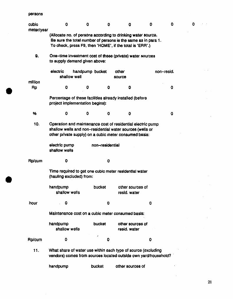
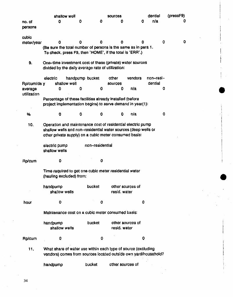
One-time investment cost of these (private) water sourcesto supply demand given above:
millionRp
electric handpumpshallow well
0 0
bucket
0
othersource
0
non-resid
0
Percentage of these facilities already installed (beforeproject implementation begins):
10.
Rp/cum
hour
Rp/cum
11.
Operation and maintenance cost of residential electric pumpshallow wells and non-residential water sources (wells orother private supply) on a cubic meter consumed basis:
electric pumpshallow wells
non-residential
Time required to get one cubic meter residential water(hauling excluded) from:
handpumpshallow wells
bucket other sources ofresid. water
0 o 0
Maintenance cost on a cubic meter consumed basis:
handpumpshallow wells
bucket other sources ofresid. water
What share of water use within each type of source (excludingvendors) comes from sources located outside own yard/household?
handpump bucket other sources of
21
shallow wells resid. water
% 0 0 0
Average distance of these water sources (outside yard/household)but used by the consumers themselves) from place of consumption:
handpump bucket other sources of
shallow wells resid. water
meter 0 0 0
Average price of water sold by vendors (carriers):
Rp/cum 0
Do you consider this price an acceptable indicator of the costof water (considering hauling cost and the cost at the sourceof the water)? If answer is yes, change indicator to "1 * and goto paragraph 12, if no write "0" and continue here.
indie. 0
Average quantity supplied by those water sources which thevendors use to purchase the water they distribute:
cum/day/source 0
Cost of that water at the source (different from price —exclude remuneration/net income of concessionaires/owners):
Rp/cum 0
Average delivery rate of vendors:cum/day/vendor 0
THIS IS THE END OF DATA INPUT FOR THE 'WITHOUT' PROJECT CASE.PLEASE PRESS CALC (F9) AND REVIEW THE RESULTS BELOW. THE ONLYPROPER WAY TO MODIFY RESULTS IS TO MODIFY THE INPUT DATA. IFFINISHED, PROCEED TO SECTION C (PARA13).
12. Economic cost of water to be replaced:
Rp/cum electric handpump bucket other vendors non-resid.shallow well source
capital 0 0 0 0 0O&M 0 0 0 0 0 0
hauling 0 0 0 0 0
22
boiling 0 0 0 0 0 0
total 0 0 0 0 0 0
C. Benefit from incremental water consumption:
13. Net incremental water use as a result of the project:
residential non-residential
cum/year 0 0
The following calculation assumes a linear relationship betweenwater demand and price and is based on a so-called(high-quantity; low-price) reference point of the residentialwater demand function, estimated as
(100 cum/year/capita; 300 rupiah/cum)If you wish to change the coordinates of this point, do it now:
( 100 ; 300 ) (AND PRESS CALC/F9/)
Average economic value of incremental water:
residential non-residential
Rp/cum 0 0 (includes consumer surplus)
D. Results:
14. Net benefit of the project (in one year):
mill.Rp 0
Net benefit/investment ratio (over the lifetime /25years/ ofthe project — may be used for ranking):
% 0
Economic internal rate of return (should not be used to rankprojects):
% ERR
(If the value above is 'ERR* or a large negative numberpress ALT and type E simultaneously.)
E. IF YOU WISH TO PRINT THE RESULTS OF YOUR WORK, PLEASE SUPPLYTHE FOLLOWING INFORMATION:
Project location:
23
Ii
Province: !Kabupaten: jKecamatan: ;
Desa: j
Number of variant tested (e.g. 1st, 2nd,etc):i
Sensitivity of results was analyzed with respect to: ji
name of variable:value of variable in this variant: |
I
PRESS ALT AND TYPE P SIMULTANEOUSLY TO BEGIN PRINTING (IF YOU \HAVE A PRINTER ON LINE AND CONNECTED TO THE COMPUTER).
THE END M
24
Annex 3: Mathematical Formulas of ECOWATl
1. In paragraph 7:
Capital cost of piped water = INV0.1/OUTPwhere INV is the present value (in year 1) of investments
OUTP is the piped water delivered by project in year 1
Connection cost of piped water = CONN*0.1/OUTPwhere CONN is the present value of connection costs
-Hauling cost of water from public standpipes =a) if vendors carry the water:
= VENT/VEND + CONT/CONDb) if consumers carry the water:
= (DISP/40 + STPD)*TIMEwhere VENT is the opportunity cost of vendor services
VEND delivery rate of vendorsCONT is the opp. cost of standpipe operator servicesCOND delivery rate of standpipesDISP distance of standpipes from place of consumptionSTPD time to get 1 cu. m. from standpipeTIME value of time
Boiling cost of water =a) if project has no impact on boiling: 0b) if project makes a difference:
where KERP is the kerosene priceBQUA is the quantity boiled daily/capitaPERS is the number of persons relying on piped waterNB05 is the percentage of people giving up boiling in year 5NB10 is the percentage of people giving up boiling in year 10
2. In paragraph 12:
Capital cost of water to be replaced = 0.11 * INVN**(UNST/100)/WREP
where INVN is the total investment cost of non-piped sourcesINST is the % already installedWREP is the water to be replaced (quantity)
O&M cost of water from handpump, bucket systems and other sources :MAIN + H0UR*TIME
where MAIN is the maintenance cost/cu.m.HOUR is the time required to get 1 cu.m. water
25
Hauling cost of water from handpumps, bucket systems and other sources *SHWU/100*DISR/40*TIME
where SHWU is the share of water use coming from outside the yardDISR is the distance from place of consumption
Capital & O&M & hauling cost of water from vendors =a) if vendor price is accepted = VPRb) if vendor price is not accepted =
COST + CONT/SOUD + VENT/VENDRwhere COST is the cost of water at the source
SOUD is the delivery rate of the water sourceVENDR is the delivery rate of vendors carrying water to be replaced
VPR is the vendor price
Boiling cost of water to be replaced =a) if project has an impact on boiling
« S»KERP/200*BQUA*365*PERSR/WREPb) otherwise 0where PERSR is the number of persons relying on the water source.
3. In paragraph 13:
incremental non-residential water use = OUTN-WRNwhereOUTN is the water delivered to non-residential customers by the project.
WRN is the water use of non-residential customers replaced by the projectincremental residential water use = (OUTP-OUTN)-(WREP-WRN)
-average economic value of incremental residential water =(MGW+MGW0)/2
where MGW is the marginal value of water, with projectMWGO is the marginal value of water, without project
and MGWO = sum^MGWO, • WREP,)whereMGWO, is the marginal value of water from ith source, defined as O&M + handling + boiling cost
or vendor price (in the case of vendors) + boiling costand MGW = (MGWO * (REFQ-WCWO-WCWI) + REFP * WCWI)/(REFQ-WCWO)where(REFQ, REFP) are the coordinates of the (high quantity; low price) reference point on the demand
curve;WCWO is the water consumption per capita, without projectWCWI is the incremental water consumption per capita, with project
average economic value of incremental non-residential water =a) if the net incremental water use is positive = (CNRP+CNRR)/2
whereCNRP is the economic cost of non-residential piped water defined in para. 7.CNRR is the total cost of non-residential water, without project, includes sunk capital cost
b)if the net incremental water use is zero or negative: = CNRR
26
4. In paragraph 14:
-net benefit of the project = INCR * VALR + INCN • VALN + sum^CWWO •WRQ,) - sum.fCPWj * OUTP,)
where INCR is the net incremental water use of residential customersVALR is the value of incremental residential water defined in para. 13.
INCN is the net incremental water use of non-residential customersVALN is the value of incremental non-residential water defined in para. 13.
CWWO, is the economic cost of the ith source of water defined in para. 12.WRQ, is the quantity of the ith source of water to be replaced
CPWj is the economic cost of the 7th type of piped water defined in para. 7.OUTPj is the quantity of the jth type of piped water delivered
-economic internal rate of return is calculated on the basis of atime series of data describing the impact of the project from year (-4) to year (25). The first fivenumbers describe the annual net investment costs, the sixth number (year 1) is equal to therecalculated annual benefits (to avoid double counting, capital costs are eliminated) minus thescheduled connection costs, the next 24 numbers are all equal to the recalculated annual netbenefits.
27
Annex 4: Introduction to EC0WAT2
The following section shows a printed version ofEC0WAT2, a program designed to carry out economicanalysis of water supply projects in Indonesia. If theproject is small (less than two billion rupiah investmentcost), a simplified version of EC0WAT2-calledECOWATl-should be used, since it requires substan-tially less input from the user. EC0WAT2 is a Lotus 123working file, which contains subroutines-so-called mac-ros~that calculate conveniently and prints the results in astandard format.
Determining the economic viability of a projectrequires affirmative answers to two questions. Is thepresent value of net benefits (NPV) of the project posi-tive?, and Is the present value of net benefits at least ashigh as the NPV of any mutually exclusive project alter-native? Looking at a new piped water supply system or atthe extension of an already existing system, the suppliedquantity of water as a result of the implemented projectcan be divided into two parts: one part replaces theprevious source and quantity of water use (wells, springs,rivers) and the other part is a net increase in the waterconsumption. Benefit from the replacement part is equalto the cost savings (actual payments plus own labor) ofconsumers who no longer need to use other sources ofwater supply. Benefit from the incremental water use isequal to the consumers* willingness to pay, which can bedetermined by estimating the area under the consumers'water demand curve. When both parts of the benefits arequantified, the net benefits of the project can be calcualtedby adding them together and subtracting the cost of newwater supply. This answers the first question. Anaffirmative answer to the second question should resultfrom careful project design, which has two importantcomponents: to select a least-cost solution for raw water
intake, storage, and treatment; and to extend the distribu-tion system towards those consumers who, without theproject, would have the highest-cost water supply (includ-ing the costs of their own labor in carrying the water) fromalternative sources.
ECO WAT2 requires data that describe the watersupply/demand situation every five years for the 25 yearsafter project completion. Data input is divided into twoparts: the first part refers to the "WITH" project, thesecond to the "WITHOUT" project alternatives. Calcu-lations are based on constant prices, linear interpolation,and a 10% (real) social rate of interest. ECO WAT2 is mostuseful if applied at an early stage of project design.Sensitivity analysis of different design alternatives willhelp to choose a design that maximizes the expected neteconomic benefits.
The following pages show what appears on thecomputer screen when working with EC0WAT2. Theyare not a substitute for the program itself but demonstratethe nature of information required to carry out the analy-sis. A survey of water use in the project implementationarea is the most important requirement before using theprogram.
Comments are welcome. Please contact LaszloLovei at (202) 473-2772.
28
ECONOMIC ANALYSIS OF WATER SUPPLY PROJECTS — INDONESIA
Year(O) refers to the year of project completion — everything,with the possible exception of connections, is installed.Input data in the highlighted/coloured areas. To reach a para-graph directly, press F5 and type PARAx , when x is the numberyou want. To see the results, press F5 and type RESULT. Arrowkeys move the cell pointer.
A.1.
Year(1)
no. ofpersons
cubicmeter/year
Year(6)
no. ofpersons
cubicmeter/year
Year(11)
no. ofpersons
cubicmeter/year
Year(16)
no. ofpersons
cubicmeter/year
Year(21)
no. ofpersons
'WITH' project situation:Population served and piped water
house yardconnection
0
0
house yardconnection
0
0
house yardconnection
0
0
house yardconnection
0
0
house yardconnection
0
0
0
0
0
0
0
0
0
0
publicstandpipe
0
0
publicstandpipe
0
0
publicstandpipe
0
0
publicstandpipe
0
0
publicstandpipe
0
delivered by the
non-resid.
n/a
0
non-resid.
n/a
0
non-resid.
n/a
0
non-resid.
n/a
0
non-resid.
n/a
project:
total
total
total
total
total
(press F9)
0
0
(press F9)
0
0
(press F9)
0
0
(press F9)
0
0
(press F9)
0
29
cubic 0 0 0 0 0meter/year
Year(26) house yard public non- total (press F9)connection standpipe resid.
no. of 0 0 0 n/a 0persons
cubic 0 0 0 0 0meter/year
2. Investment cost (connection excluded) on constant prices:total
totalMRp year(1) year(6) year(11) year(16) year(21) year(26) value
in year(O)house 0 0 0 0 0 0 0
yard 0 0 0 0 0 0 0
standpipe 0 0 0 0 0 0 0
non-res. 0 0 0 0 0 0 0
4. Operation and maintenance cost of supply system (includingcompany overhead cost) on a cubic meter delivered basis:
rupiah/cub. met. 0
5. Do water vendors or the consumers themselves carry the waterfrom standpipes to the place of consumption ? (if answer isconsumers, change indicator to " 1 " , if vendors, leave as "0" )
30
vendorindie.
concess.indie.
Are there — or are there going to be — public standpipe/hydrant operators ? (if the answer is no, change the indicatorto "1 '.otherwise leave as "0")
cum/day/vendor
Rp/day/vendor
Estimated delivery rate of vendors (if no information,use 2 cum/day/vendor):
Opportunity cost of vendor labour (may be different from theirnet income as a result of monopoly or restricted entry — if noInformation, use Rp 2500/day/vendor):
cum/day/standpipe
Rp/day/cone.
Average delivery rate of standpipes:
Opportunity cost of standpipe/hydrant operator services (maybe different from their net income as a result of a monopoly— if no information, use Rp 2500/day/concessionaire):
hour
meter
Average time required to get 1 cubic meter water from standpipe(hauling excluded):
Average distance from standpipes to those households which relyon water from standpipes:
Rp/hour
6.
boilingindie.
Value of private time (if no information, Rp150/hour inJava/Bali, Rp200/hour in the Outer islands is proposed):
Did local people boil the drinking/cooking water before projectimplementation ? (if the answer is yes, change the indicator to " 1 " , no" 1 " , if no write "0")
31
boilingindie.
liter/capita/day
Rp/liter
7.
Do you assume project will make a difference in boiling habitsover time ? (if answer is yes, change indicator to " 1 " , if nowrite "0")
What percentage of population served by piped water will drinkthe water without boiling as a result of the project afterimplementation is completed /year(O)/?
Average quantity boiled daily before project implementation (ifno information use 2 liter/capita/day):
Price of kerosene sold by street vendors:
THIS IS THE END OF DATA INPUT FOR THE 'WITH1 PROJECT CASE.PLEASE PRESS CALC (F9) AND REVIEW THE RESULTS BELOW. THE ONLYPROPER WAY TO MODIFY RESULTS IS TO MODIFY THE INPUT DATA. IFFINISHED, PROCEED TO THE 'WITHOUT' CASE (PARAS).
Variable cost of piped water in year(1):
Rp/cum
O&Mhaulingboiling
house yardconnection
000
000
publicstandpipe
000
non-resid.
000
total 0 0 0 0
Capital cost of piped water (connection cost excluded):
Rp/cum 0
Connection cost of piped water (average over time):
house yardconnection
public non-standpipe resid.
Rp/cum
32
electric handpump bucket other vendors non-resi-shallow well sources dential
0 0 0 0 O n / a
total(pressF9)
0
B. 'WITHOUT1 project situation:
8. Water use of the consumers (project beneficiaries defined inpara.1.) to be replaced by the project:
(allocate no. of persons according to drinking water source)
year(1) electric handpump bucket other vendors non-resi- totalshallow well sources dential (pressF9)
no. of 0 0 0 0 0 n/a 0persons
cubicmeter/year 0 0 0 0 0 0 0
year(6)
no. ofpersons
cubicmeter/year
year(H)
no. ofpersons
cubicmeter/year
year(i6)
no. ofpersons
cubicmeter/year
year(21)
no. ofpersons
cubicmeter/year 0 0 0 0 0 0
year(26) electric handpump bucket other vendors non-resi- total
electric handpump bucket other vendors non-resi-shallowwell sources dential
0 0 0 0 O n / a
total(pressF9)
electric handpump bucket other vendors non-resi-shallow well sources dential
0 0 0 0 O n / a
total(pressF9)
0
electric handpump bucket other vendors non-resi-shallow well sources dential
0 0 0 0 0 n/a
total(pressF9)
33
no. ofpersons
cubicmeter/year
shallow well0
0
0
0
0
0
sources0
0
0
0
dentialn/a
0
(pressF9)0
0
9.
Rp/cum/daaverageutilization
10.
(Be sure the total number of persons is the same as in para 1.To check, press F9, then 'HOME', if the total is 'ERR'.)
One-time investment cost of these (private) water sourcesdivided by the daily average rate of utilization:
electric handpump bucket other vendors non-resi-y shallow well sources dential
0 0 0 0 n/a 0
Percentage of these facilities already installed (beforeproject implementation begins) to serve demand in year(1):
n/a
Operation and maintenance cost of residential electric pumpshallow wells and non-residential water sources (deep wells orother private supply) on a cubic meter consumed basis:
electric pumpshallow wells
non-residential
Rp/cum
Time required to get one cubic meter residential water(hauling excluded) from:
handpumpshallow wells
bucket other sources ofresid. water
hour
Maintenance cost on a cubic meter consumed basis:
handpumpshallow wells
bucket other sources ofresid. water
Rp/cum
11. What share of water use within each type of source (excludingvendors) comes from sources located outside own yard/household?
handpump bucket other sources of
34
shallow wells resid. water
Average distance of these water sources (outside yard/householdbut used by the consumers themselves) from place of consumption:
handpumpshallow wells
bucket other sources ofresid. water
meter
Rp/cum
indie.
cum/day/source
Rp/cum
cum/day/vendor
12.
Rp/cum
O&Mhaulingboiling
Average price of water sold by vendors (carriers):
0
Do you consider this price an acceptable indicator of the costof water (considering hauling cost and the cost at the sourceof the water)? If answer is yes, change indicator to " 1 " and goto paragraph 12, if no write "0" and continue here.
Average quantity supplied by those water sources which areused by vendors to purchase the water they distribute:
Cost of that water at the source (different from price —exclude remuneration/net income of concessionaires/owners):
Average delivery rate of vendors:
THIS IS THE END OF DATA INPUT FOR THE 'WITHOUT' PROJECT CASE.PLEASE PRESS CALC (F9) AND REVIEW THE RESULTS BELOW. THE ONLYPROPER WAY TO MODIFY RESULTS IS TO MODIFY THE INPUT DATA. IFFINISHED, PROCEED TO SECTION C (PARA13).
Variable cost of water to be replaced in year(1):
electric handpump bucket other vendors non-resi-shallow well sources dential
000
000
000
000
000
35
total 0 0 0 0 0 0
C. Benefit from incremental water consumption:
13. Net incremental water use as a result of the project in year(1):
residential non-residential
cum/year 0 0
The following calculation assumes a linear relationship betweenresidential water demand and price and is based on a so-called(high-quantity ; low-price) reference point of the residentialwater demand function, estimated in year(0) as
(100 cum/year/capita ; 300 rupiah/cum)If you wish to change the coordinates of this point, do it now:
( 100 ; 300 ) (AND PRESS CALC/F9/)
Water demand depends on income, too. Even for the same price,households buy more water, if their income is higher. What isyour estimate of the per capita real income, if year(0)=100 ?
F9 AGAIN)Average economic value of incremental water:residential non-residential(year(1)) (same in every year)
Rp/cum 0 0 (includes consumer surplus)
D. Results:
14. Net present value of the project:
mill.Rp 0
Net benefit/investment ratio (may be used for ranking):
% 0
Economic internal rate of return (should not be used to rankprojects):
% ERR
(If the value above is 'ERR' press ALT and type Esimultaneously.)
36
E. IF YOU WISH TO PRINT THE RESULTS OF YOUR WORK, PLEASE SUPPLYTHE FOLLOWING INFORMATION:
Project location:
Province:Kabupaten:Kecamatan:
Desa:
Number of variant tested (e.g. 1st, 2nd,etc):
Sensitivity of results was analyzed with respect to:
name of variable:value of variable in this variant:
PRESS ALT AND TYPE P SIMULTANEOUSLY TO BEGIN PRINTING (IF YOUHAVE A PRINTER ON LINE AND CONNECTED TO THE COMPUTER).
THE END
37
Policy Research Working Paper Series
WPS977
WPS978
WPS979
WPS980
WPS981
WPS982
WPS983
WPS984
WPS985
WPS986
WPS987
WPS988
WPS989
WPS990
WPS991
Title Author
Income Security for Old Age: Estelle JamesConceptual Background and Major Issues
How Restricting Carbon Dioxideand Methane Emissions Would Affecthe Indian Economy
Economic Growth and theEnvironment
The Environment: A New Challengefor GATT
After Socialism and Dirigisme:Which Way?
Microeconomics of Transformationin Poland: A Survey of StateEnterprise Responses
Legal Reform for Hungary's PrivateSector
Barriers to Portfolio Investmentsin Emerging Stock Markets
Regional Integration, Old andNew
The Administration of Road UserTaxes in Developing Countries
How the Epidemiological TransitionAffects Health Policy Issues inThree Latin American Countries
Economic Valuation and theNatural World
The Indian Trade Regime
Protection and Industrial Structurein India
Environmental Costs of NaturalRaeniircfl Commorlitins- Mannituda
Charles R. Blitzert R. S. Eckaus
Supriya LahiriAlexander Meeraus
Dennis Anderson
Piritta Sorsa
Andres Solimano
Brian PintoMarek BelkaStefan Krajewski
Cheryl W. GrayRebecca J. HansonMichael Heller
Asli Demirguc-KuntHarry Huizinga
Jaime de MeloClaudio MontenegroArvind Panagariya
Roy Bahl
Jose Luis BobadillaCristina de A. Possas
David Pearce
M. Ataman Aksoy
M. Ataman AksoyFrancois M. Ettori
Margaret E. Slade
Date
September 1992
September 1992
September 1992
September 1992
September 1992
September 1992
October 1992
October 1992
October 1992
October 1992
October 1992
October 1992
October 1992
October 1992
October 1992
Contactfor paper
D. Evans37496
WDR Office31393
WDR Office31393
WDR Office31393
S. Fallon37947
S. Husain37139
R. Martin39065
W. Patrawimolpon37664
D. Ballantyne37947
J. Francis-O'Connor35205
O. Nadora31091
WDR Office31393
R. Matenda35055
R. Matenda35055
WDR Office31393
and Incidence
Policy Research Working Paper Series
Title Author
WPS992
WPS993
WPS994
WPS995
WPS996
WPS997
WPS998
WPS999
Regional Integration in Sub-Saharan Faezeh ForoutanAfrica: Experience and Prospects
An Economic Analysis of CapitalFlight from Nigeria
S. Ibi Ajayi
Textiles and Apparel in NAFTA: Geoffrey BannisterA Case of Constrained Liberalization Patrick Low
Recent Experience with Commercial Stijn ClaessensBank Debt Reduction Ishac Diwan
Eduardo Fernandez-Arias
Strategic Management of Population Michael H. BernhartPrograms
How Financial Liberalization in John R. HarrisIndonesia Affected Firms' Capital Fabio SchiantarelliStructure and Investment Decisions Miranda G. Siregar
What Determines Demand for Freight Esra BennathanTransport? Julie Fraser
Louis S. Thompson
Stopping Three Big Inflations(Argentina, Brazil, and Peru)
Miguel A. KiguelNissan Liviatan
WPS1000 Why Structural Adjustment Has Not Ibrahim A. ElbadawiSucceeded in Sub-Saharan Africa Dhaneshwar Ghura
Gilbert Uwujaren
WPS1001 Have World Bank-Supported Ibrahim A. ElbadawiAdjustment Programs Improved EconomicPerformance in Sub-Saharan Africa?
WPS1002 World Energy Subsidies and GlobalCarbon Emissions
WPS1003 Rent-Sharing in the Multi-FibreArrangement: Evidence from U.S.-Hong Kong Trade in Apparel
WPS1004 Family Planning Programs in Sub-Saharan Africa: Case Studies fromGhana, Rwanda, and the Sudan
WPS1005 An Approach to the EconomicAnalysis of Water Supply Projects
Bjorn LarsenAnwar Shah
Kala KrishnaLing Hui Tan
Regina McNamaraTherese McGinnDonald LauroJohn Ross