AN APPROXIMATION ALGORITHM FOR COUNTING CONTINGENCY TABLES Alexander Barvinok, Zur Luria, Alex Samorodnitsky, and Alexander Yong March 2008 Abstract. We present a randomized approximation algorithm for counting con- tingency tables, m × n non-negative integer matrices with given row sums R = (r 1 ,...,r m ) and column sums C =(c 1 ,... ,c n ). We define smooth margins (R, C) in terms of the typical table and prove that for such margins the algorithm has quasi- polynomial N O(ln N) complexity, where N = r 1 + ··· + r m = c 1 + ··· + c n . Various classes of margins are smooth, e.g., when m = O(n), n = O(m) and the ratios be- tween the largest and the smallest row sums as well as between the largest and the smallest column sums are strictly smaller than the golden ratio (1 + √ 5)/2 ≈ 1.618. The algorithm builds on Monte Carlo integration and sampling algorithms for log- concave densities, the matrix scaling algorithm, the permanent approximation algo- rithm, and an integral representation for the number of contingency tables. 1. Introduction Let R =(r 1 ,...,r m ) and C =(c 1 ,...,c n ) be positive integer vectors such that m i=1 r i = n j =1 c j = N. A contingency table with margins (R,C ) is an m × n non-negative integer matrix D =(d ij ) with row sums R and column sums C : n j =1 d ij = r i for i =1,...,m m i=1 d ij = c j for j =1,...,n. Key words and phrases. Contingency tables, randomized approximation algorithm, matrix scaling algorithm, permanent approximation algorithm. Typeset by A M S-T E X 1
Transcript
AN APPROXIMATION ALGORITHM FOR
COUNTING CONTINGENCY TABLES
Alexander Barvinok, Zur Luria, Alex
Samorodnitsky, and Alexander Yong
March 2008
Abstract. We present a randomized approximation algorithm for counting con-
tingency tables, m × n non-negative integer matrices with given row sums R =(r1, . . . , rm) and column sums C = (c1, . . . , cn). We define smooth margins (R, C)
in terms of the typical table and prove that for such margins the algorithm has quasi-
polynomial NO(ln N) complexity, where N = r1 + · · · + rm = c1 + · · · + cn. Variousclasses of margins are smooth, e.g., when m = O(n), n = O(m) and the ratios be-
tween the largest and the smallest row sums as well as between the largest and the
smallest column sums are strictly smaller than the golden ratio (1 +√
5)/2 ≈ 1.618.The algorithm builds on Monte Carlo integration and sampling algorithms for log-
concave densities, the matrix scaling algorithm, the permanent approximation algo-rithm, and an integral representation for the number of contingency tables.
1. Introduction
Let R = (r1, . . . , rm) and C = (c1, . . . , cn) be positive integer vectors such that
m∑
i=1
ri =
n∑
j=1
cj = N.
A contingency table with margins (R,C) is an m × n non-negative integer matrixD = (dij) with row sums R and column sums C:
n∑
j=1
dij = ri for i = 1, . . . , m
m∑
i=1
dij = cj for j = 1, . . . , n.
Key words and phrases. Contingency tables, randomized approximation algorithm, matrixscaling algorithm, permanent approximation algorithm.
Typeset by AMS-TEX
1
Let #(R,C) denote the number of these contingency tables.There is interest in the study of #(R,C), due to connections to statistics, com-
binatorics and representation theory, see, e.g., [Go76], [DE85], [DG95], [D+97],[Mo02], [CD03], [L+04], [B+04], [C+05] and the references therein. However, sinceenumerating #(R,C) is a #P -complete problem even for m = 2 [D+97], one doesnot expect to find polynomial-time algorithms (nor formulas) computing #(R,C)exactly. As a result, attention has turned to the open problem of efficiently esti-mating #(R,C).
We present a randomized algorithm for approximating #(R,C) within a pre-scribed relative error. Based on earlier numerical studies [Yo07] [B+07], we conjec-ture that its complexity is polynomial in N . We provide further evidence for thishypothesis: we introduce “smooth margins” (R,C) where the entries of the typical
table are not too large, and among r1, . . . , rm, c1, . . . , cn there are no “outliers”.Our main result is that smoothness implies a quasi-polynomial NO(log N) com-plexity bound on the algorithm. More precisely, we approximate #(R,C) withinrelative error ǫ > 0 using (1/ǫ)O(1)NO(ln N) time in the unit cost model, providedǫ≫ 2−m + 2−n.1
The class of smooth margins captures a number of interesting subclasses. Inparticular, this work applies to the case of magic squares (where m = n and ri =cj = t for all i, j), extending [B+07]. More generally, smoothness includes the casewhen the ratios m/n and n/m are bounded by a constant fixed in advance while theratios between the largest and the smallest row sums as well as between the largestand the smallest column sums are smaller than the golden ratio
(
1 +√
5)
/2 ≈1.618. These and others examples are explicated in Section 3. See Section 1.4 forcomparisons to the literature.
(1.1) An outline of the algorithm. Our algorithm builds on the techniqueof rapidly mixing Markov chains and, in particular, on efficient integration andsampling from log-concave densities, as developed in [AK91], [F+94], [FK99], [LV06](see also [Ve05] for a survey), the permanent approximation algorithm [J+04], thestrongly polynomial time algorithm for matrix scaling [L+00], and the integralrepresentation of #(R,C) from [Ba08].
Let ∆ = ∆m×n ⊂ Rmn be the open (mn− 1)-dimensional simplex of all m × n
positive matrices X = (xij) such that∑
ij
xij = 1.
Let dX be Lebesgue measure on ∆ normalized to the probability measure. Anintegral representation for #(R,C) was found in [Ba08]:
(1.1.1) #(R,C) =
∫
∆
f(X) dX,
1If an exponentially small relative error ǫ = O`
2−m + 2−n´
is desired, one has an exact
dynamic programming algorithm with NO(m+n) = (1/ǫ)O(ln N) quasi-polynomial complexity.
2
where f : ∆ −→ R+ is a certain continuous function that factors as
(1.1.2) f = pφ,
wherep(X) ≥ 1 for all X ∈ ∆
is a function that “does not vary much”, and φ : ∆ −→ R+ is continuous andlog-concave, that is,
φ(αX + βY ) ≥ φα(X)φβ(Y ) for all X, Y ∈ ∆ and
for all α, β ≥ 0 such that α+ β = 1.
Full details about f and its factorization are reviewed in Section 2.For any X ∈ ∆, the values of p(X) and φ(X) are computable in time polynomial
in N . Given ǫ > 0, the value of p(X) can be computed, within relative error ǫ intime polynomial in 1/ǫ and N , by a randomized algorithm of [J+04]. The value ofφ(X) can be computed, within relative error ǫ in time polynomial in ln(1/ǫ) andN , by a deterministic algorithm of [L+00].
The central idea of this paper is to define smooth margins (R,C) so that matricesX ∈ ∆ with large values of p(X) do not contribute much to the integral (1.1.1).Our main results, precisely stated in Section 3, are that for smooth margins, there isa threshold τ = N δ ln N for some constant δ > 0 (depending on the class of marginsconsidered) such that if we define the truncation p : ∆ −→ R+ by
p(X) =
p(X) if p(X) ≤ τ
τ if p(X) > τ
then
(1.1.3) #(R,C) =
∫
∆
p(X)φ(X) dX ≈∫
∆
p(X)φ(X) dX
where “≈” means “approximates to within an O (2−n + 2−m) relative error” (infact, rather than base 2, any constant M > 1, fixed in advance, can be used). Weconjecture that one can choose the threshold τ = NO(1), which would make thecomplexity of our algorithm polynomial in N .
The first step (and a simplified version) of our algorithm computes the integral
(1.1.4)
∫
∆
φ(X) dX
using any of the aformentioned randomized polynomial time algorithms for inte-
grating log-concave densities; these results imply that this step has polynomial in N3
complexity. By (1.1.3) it follows that for smooth (R,C) the integral (1.1.4) approx-imates #(R,C) within a factor of NO(ln N). This simplified algorithm is suggestedin [Ba08]; an implementation that utilizes a version of the hit-and-run algorithm of[LV06], together with numerical results is described in [Yo07] and [B+07].
Next, our algorithm estimates (1.1.3) within relative error ǫ using the aformen-tioned randomized polynomial time algorithm for approximating the permanent ofa matrix, and any of those for sampling from log-concave densities. Specifically, letν be the probability measure on ∆ with the density proportional to φ. Thus,
∫
∆
p(X)φ(X) dX =
(∫
∆
p dν
)(∫
∆
φ(X) dX
)
.
The second factor is computed by the above first step, while the first factor isapproximated by the sample mean
(1.1.5)
∫
∆
p dν ≈ 1
k
k∑
i=1
p(Xi),
where X1, . . . , Xk ∈ ∆ are independent points sampled at random from measure ν.Since 1 ≤ p(X) ≤ τ , the Chebyshev inequality implies that to achieve relative errorǫ with probability 2/3 it suffices to sample k = O
(
ǫ−2τ2)
= ǫ−2NO(ln N) points in(1.1.5).
The results of [AK91], [F+94], [FK99], and [LV06] imply that for any given ǫ > 0one can sample independent points X1, . . . , Xk from a distribution ν on ∆ suchthat
|ν(S) − ν(S)| ≤ ǫ for any Borel set S ⊂ ∆.
in time linear in k and polynomial in ǫ−1 and N . Replacing ν by ν in (1.1.5)introduces an additional relative error of ǫτ = ǫN δ ln N , handled by choosing asmaller ǫ = O
(
N−δ ln N)
.
(1.2) An optimization problem, typical tables and smooth margins. Wewill define smoothness of margins in terms of a certain convex optimization problem.
Let P = P(R,C) be the transportation polytope of m× n non-negative matricesX = (xij) with row sums R and column sums C. On the space R
mn+ of m × n
non-negative matrices define
g(X) =∑
ij
(
(xij + 1) ln (xij + 1) − xij lnxij
)
for X = (xij) .
The following optimization problem plays an important role in this paper:
(1.2.1) Maximize g(X) subject to X ∈ P.
It is easy to check that g is strictly concave and hence attains its maximum on Pat a unique matrix X∗ =
(
x∗ij)
, X∗ ∈ P that we call the typical table.4
An intuitive explanation for the appearance of this optimization problem, andjustification for the nomenclature “typical” derives from work of [B07b] (relevantparts are replicated for convenience, in Section 4, see specifically Theorem 4.1). Inshort, X∗ determines the asymptotic behavior of #(R,C).
The main requirement that we demand of smooth margins (R,C) to satisfy (seeSection 3 for unsuppressed technicalities) is that the entries of the typical table arenot too large, that is, entries x∗ij of the optimal solution X∗ =
(
x∗ij)
satisfy
maxij
x∗ij = O(s) where s =N
mn
is the average entry of the table.Viewing the typical table as interesting in its own right, one would like to under-
stand how the typical table changes as the margins vary. The optimization problembeing convex, X∗ can be computed efficiently by many existing algorithms, see, forexample, [NN94]. However, in many instances of interest, the smoothness conditioncan be checked without actually needing to solve this problem. For example, if allthe row sums ri are equal, the symmetry of the functional g under permutations ofrows implies that
x∗ij =cjm
for all i, j.
In general, the entries x∗ij stay small if the row sums ri and column sums cj do notvary much. On the other hand, it is not hard to construct examples of margins(R,C) for n-vectors R and C such that n ≤ ri, cj ≤ 3n and some of the entries x∗ijare large, in fact linear in n. Another one of our results (Theorem 3.5) gives upperand lower bounds for x∗ij in terms of (R,C).
(1.4) Comparisons with the literature. Using the Markov Chain Monte Carloapproach, Dyer, Kannan, and Mount [D+97] count contingency tables when R andC are sufficiently large, that is, if ri = Ω
(
n2m)
and cj = Ω(
m2n)
for all i, j. Theirrandomized (sampling) algorithm approximates #(R,C) within any given relativeerror ǫ > 0 in time polynomial in ǫ−1, n, m, and
∑
i log ri +∑
j log cj (the bit
size of the margins). Subsequently, Morris [Mo02] obtained a similar result for thebounds ri = Ω
(
n3/2m lnm)
and cj = Ω(
m3/2n lnn)
. These results are based onfact that for large margins, the number of contingency tables is well-approximatedby the volume of the transportation polytope P(R,C) (contingency tables beingthe integer points in this polytope). More generally, Kannan and Vempala [KV99]show that estimating the number integer points in a d-dimensional polytope withm facets reduces to computing the volume of the polytope (a problem, for whichefficient randomized algorithms exist, see [Ve05] for a survey) provided the polytopecontains a ball of radius d
√logm.
When the margins ri, cj are very small, that is, bounded by a constant fixedin advance) relative to the sizes m and n of the matrix, Bekessy, Bekessy, andKomlos [B+72] obtain an efficient and precise asymptotic formula for #(R,C).
5
Their formula exploits the fact in this case, the majority of contingency tables haveonly entries 0, 1, and 2. Alternatively, in this case one can exactly compute #(R,C)in time polynomial in m+n via a dynamic programming algorithm. More recently,Greenhill and McKay [GM07] gave a computationally efficient asymptotic formulafor a wider class of sparse margins (when ricj = o(N2/3)).
Also using the dynamic programming approach, Cryan and Dyer [CD03] con-struct a randomized polynomial time approximation algorithm to compute #(R,C),provided the number of rows is fixed; see [C+06] for sharpening of the results.
It seems that the most resilient case of computing #(R,C) is where both m andn grow, and the margins are of moderate size, e.g., linear in the dimension. Re-cently, Canfield and McKay [CM07] found a precise asymptotic formula for #(R,C)assuming that all row sums are equal and all column sums are equal. However, forgeneral margins no such formula is known, even conjecturally.
We remark that our notion of smooth margins includes all of the above regimes,except for that of large margins.
Summarizing, although our complexity bounds do not improve on the algorithmsin the above cases, our algorithm is provably computationally efficient (quasi-polynomial in N) for several new classes of margins, which include cases of growingdimensions m and n and moderate size margins R and C.
2. The integral representation for
the number of contingency tables
We now give details of the integral representation (1.1.1). To do this, we express#(R,C) as the expectation of the permanent of a random N × N matrix. Recallthat the permanent of an N ×N matrix A is defined by
perA =∑
σ∈SN
N∏
i=1
aiσ(i),
where SN is the symmetric group of the permutations of the set 1, . . . , N. Thefollowing result was proved in [Ba08].
(2.1) Theorem. For an m × n matrix X = (xij), let A(X) be the N × N block
matrix A(X) whose the (i, j)-th block is the ri × cj submatrix filled with xij, for
i = 1, . . . , m and j = 1, . . . , n. Then
(2.1.1)perA(X)
r1! · · · rm!c1! · · · cn!=
∑
D=(dij)
∏
ij
xdij
ij
dij !,
where the sum is over all non-negative integer matrices D = (dij) with row sums
R and column sums C.
6
Let Rmn+ be the open orthant of positive m× n matrices X. Then
#(R,C) =1
r1! · · · rm!c1! · · · cn!
∫
Rmn+
perA(X) exp
−∑
ij
xij
dX,
where dX is the Lebesgue measure on Rmn+ .
In the case that ri = a and cj = b for all i, j, the expansion (2.1.1) was firstobserved by Bang and then used by Friedland [Fr79] in his proof of a weaker formof the van der Waerden conjecture; see Section 7.1 and references there.
Since the function X 7−→ perA(X) is a homogeneous polynomial of degree N ,one can express #(R,C) as an integral over the simplex. The following corollarywas also obtained in [Ba08].
(2.2) Corollary. Let ∆ = ∆m×n ⊂ Rmn be the open simplex of positive m × n
matrices X = (xij) such that∑
ij xij = 1. Then
#(R,C) =(N +mn− 1)!
(mn− 1)!
1
r1! . . . rm!c1! · · · cn!
∫
∆m×n
perA(X) dX,
where dX is the Lebesgue measure on ∆m×n normalized to the probability measure.
Hence in the integral representation (1.1.1), we define the function f by
f(X) =(N +mn− 1)!
(mn− 1)!
1
r1! . . . rm!c1! · · · cn!perA(X)
=(N +mn− 1)!
(mn− 1)!
∑
D=(dij)
∏
ij
xdij
ij
dij !,
where A(X) is the block matrix of Theorem 2.1 and the sum is over all contingencytables D with margins (R,C).
(2.3) Matrix scaling and the factorization of f . To obtain the factorization(1.1.2), where φ : ∆ −→ R+ is a log-concave function and p : ∆ −→ R+ is afunction which “does not vary much”, we employ the idea of matrix scaling, see[Si64], [MO68], [KK96], Chapter 6 of [BR97], and [L+00]: Let X = (xij) be apositive m × n matrix. Then there exists a unique m × n matrix Y with the rowsums R = (r1, . . . , rm), column sums C = (c1, . . . , cn), and such that
xij = yijλiµj for all i, j
and some positive λ1, . . . , λm, µ1, . . . , µn. The numbers λi and µj are unique upto a re-scaling λi 7−→ λiτ , µj 7−→ µjτ
−1. Note that if we divide the entries in the(i, j)-th block of the matrix A(X) of Theorem 2.1 by ricjλiµj , we obtain a positive
7
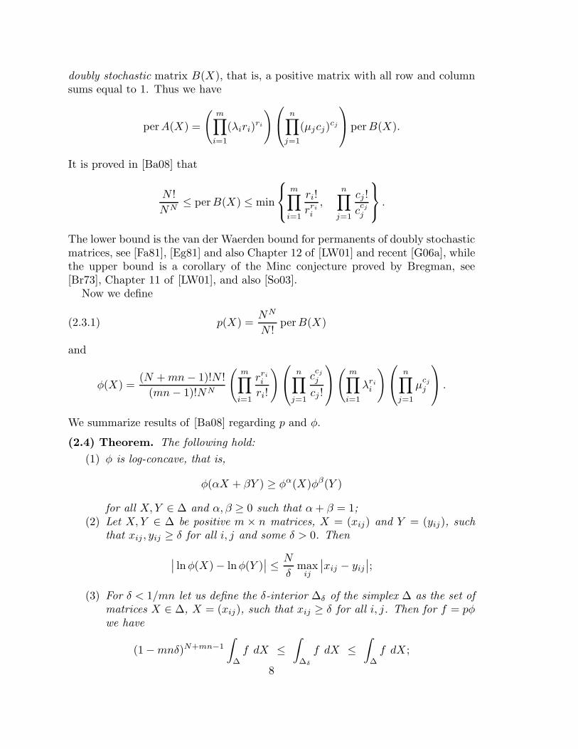
doubly stochastic matrix B(X), that is, a positive matrix with all row and columnsums equal to 1. Thus we have
perA(X) =
(
m∏
i=1
(λiri)ri
)
n∏
j=1
(µjcj)cj
perB(X).
It is proved in [Ba08] that
N !
NN≤ perB(X) ≤ min
m∏
i=1
ri!
rri
i
,
n∏
j=1
cj !
ccj
j
.
The lower bound is the van der Waerden bound for permanents of doubly stochasticmatrices, see [Fa81], [Eg81] and also Chapter 12 of [LW01] and recent [G06a], whilethe upper bound is a corollary of the Minc conjecture proved by Bregman, see[Br73], Chapter 11 of [LW01], and also [So03].
Now we define
(2.3.1) p(X) =NN
N !perB(X)
and
φ(X) =(N +mn− 1)!N !
(mn− 1)!NN
(
m∏
i=1
rri
i
ri!
)
n∏
j=1
ccj
j
cj !
(
m∏
i=1
λri
i
)
n∏
j=1
µcj
j
.
We summarize results of [Ba08] regarding p and φ.
(2.4) Theorem. The following hold:
(1) φ is log-concave, that is,
φ(αX + βY ) ≥ φα(X)φβ(Y )
for all X, Y ∈ ∆ and α, β ≥ 0 such that α+ β = 1;(2) Let X, Y ∈ ∆ be positive m × n matrices, X = (xij) and Y = (yij), such
that xij , yij ≥ δ for all i, j and some δ > 0. Then
∣
∣ lnφ(X) − lnφ(Y )∣
∣ ≤ N
δmax
ij
∣
∣xij − yij
∣
∣;
(3) For δ < 1/mn let us define the δ-interior ∆δ of the simplex ∆ as the set of
matrices X ∈ ∆, X = (xij), such that xij ≥ δ for all i, j. Then for f = pφwe have
(1 −mnδ)N+mn−1
∫
∆
f dX ≤∫
∆δ
f dX ≤∫
∆
f dX ;
8
(4) We have
1 ≤ p(X) ≤ NN
N !min
m∏
i=1
ri!
rri
i
,
n∏
j=1
cj !
ccj
j
.
The log-concavity of function φ was first observed in [G06b]. In terms of [G06b],up to a normalization factor, φ(X) is the capacity of the matrix A(X) of Theorem2.1, see also [B07b] for a more general family of inequalities satisfied by φ. As isdiscussed in [Ba08], the matrix scaling algorithm of [L+00] leads to a polynomialtime algorithm for computing φ(X). Namely, for any given ǫ > 0 the value of φ(X)can be computed within relative error of ǫ in time polynomial in N and ln(1/ǫ) inthe unit cost model; our own experience is that this algorithm for computing φ(X)is practical, and works well for m,n ≤ 100.
Theorems 2.4 and 2.1 allow us to apply algorithms of [AK91], [F+94], [FK99],and [LV06] on efficient integration and sampling of log-concave functions. First, forany given ǫ > 1, one can compute the integral
∫
∆
φ dX
within relative error ǫ in time polynomial in ǫ−1 and N by a randomized algorithm.Second, one can sample points X1, . . . , Xk ∈ ∆ independently from a measure νsuch that
|ν(S) − ν(S)| ≤ ǫ for any Borel set S ⊂ ∆,
where ν is the measure with the density proportional to φ, in time polynomial ink, ǫ−1 and N .
The integration of p(X) raises a greater challenge. For any given ǫ > 0 one cancompute p(X) itself within relative error ǫ in time polynomial in ǫ−1 and N , usingthe permanent approximation algorithm of [J+04]. However, the upper bound ofPart (4) of Theorem 2.4 is, in the worst case, of order Nγ(m+n) for some absoluteconstant γ > 0. Therefore, a priori, to integrate p over ∆ using a sample mean,one needs too many such computations to guarantee the desired accuracy of ǫ. Ourmain observation to overcome this problem is that in many interesting cases thematrices X ∈ ∆ with large values of p(X) do not contribute much to the integral(1.1.1), so we have p(X) = NO(ln N) with high probability with respect to thedensity on ∆ proportional to f .
(2.5) Bounding p with high probability. Let us consider the projection
pr : Rmn+ −→ ∆m×n, pr(X) =X, where
X = αX for α =
∑
ij
xij
−1
.
9
Clearly, the scalings of X and X to the matrix with the row sums R and columnsums C coincide. Also, it is clear that the doubly stochastic scalings B(X) and
B(X), of matrices A(X) and A(X), respectively, also coincide. We define p(X) for
an arbitrary positive m×n matrix X by p(X) := p(X), or, equivalently, by (2.3.1).We introduce the following density ψ = ψR,C on R
mn+ by
ψ(X) =1
#(R,C)
∑
D=(dij)
∏
ij
xdij
ij
dij!e−xij , where
X = (xij) and xij > 0 for all i, j,
and the sum is over all m× n non-negative integer matrices D with the row sumsR and column sums C. We define ψ(X) = 0 if X is not a positive matrix. That ψis a probability density is immediate from Theorem 2.1.
Our goal is to show that for smooth margins (R,C), the value of p(X) is “rea-sonably small” for most X , that is,
(2.5.1) P
X ∈ Rmn+ : p(X) > N δ ln N
< κ(
2−m + 2−n)
for some constants δ > 0 and κ > 0, where the probability is measured with respectto the density ψ.
Our construction of function f in (1.1.1) implies that the push-forward of ψunder the projection pr : R
mn+ −→ ∆ is the density
1
#(R,C)f(X) for X ∈ ∆
on the simplex. Hence inequality (2.5.1) implies that for τ = N δ ln N we have
1
#(R,C)
∫
X∈∆p(X)>τ
f(X) dX < κ(
2−m + 2−n)
.
Therefore, as discussed in Section 1.1, replacing p by its truncation p introducesan O (2−n + 2−m) relative error in (1.1.3) and hence our algorithm achieves quasi-polynomial complexity.
The key idea behind inequality (2.5.1) is that the permanent of an appropriatelydefined “random” doubly stochastic matrix is very close with high probability tothe van der Waerden lower bound N !/NN ; see Lemma 5.1.
3. Main results
Now we are ready to precisely define the classes of smooth margins for whichour algorithm achieves NO(ln N) complexity.
mnbe the average value of the entries of the table. We define
r+ = maxi=1,... ,m
ri, r− = mini=1,... ,m
ri
c+ = maxj=1,... ,n
cj , c− = minj=1,... ,n
cj .
Hence r+ and c+ are the largest row and column sums respectively and r− and c−are the smallest row and column sums respectively.
For s0 > 0, call the margins (R,C) s0-moderate if s ≤ s0. In other words,margins are moderate if the average entry of the table is bounded from above.
For α ≥ 1, the margins (R,C) are upper α-smooth if
r+ ≤ αsn = αN
mand c+ ≤ αsm = α
N
n.
Thus, margins are upper smooth if the row and column sums are at most propor-tional to the average row and column sums respectively.
For 0 < β ≤ 1, the margins (R,C) are lower β-smooth if
r− ≥ βsn = βN
mand c− ≥ βsm = β
N
n.
Therefore, margins are lower smooth if the row and column sums are at leastproportional to the average row and column sums respectively.
The key smoothness condition is as follows: for α ≥ 1 we define margins (R,C)to be strongly upper α-smooth if for the typical table X∗ =
(
x∗ij)
we have
x∗ij ≤ αs for all i, j.
Note that this latter condition implies that the margins are upper α-smooth. (Also,we do not need a notion of strongly lower β smooth.)
Our main results are randomized approximation algorithms of quasi-polynomialNO(ln N) complexity when the margins (R,C) are smooth for either:
• s0-moderate strongly upper α-smooth, for some fixed s0 and α;
or
• lower β and strongly upper α-smooth, for some fixed α and β.
By the discussion of Section 2.5, the quasi-polynomial complexity claim aboutour algorithm follows from bounding on p(X) with high probability. Specifically,we have the following two results. Their proofs are argued similarly, but the secondis more technically involved.
11
(3.2) Theorem. Fix s0 > 0 and α ≥ 1. Suppose that m ≤ 2n, n ≤ 2m and let
(R,C) be s0-moderate strongly upper α-smooth margins. Let X = (xij) be a random
m×n matrix with density ψ of Section 2.5 , and let p : Rmn+ −→ R+ be the function
defined in Section 2.3. Then for some constant δ = δ(α, s0) > 0 and some absolute
constant κ > 0, we have
P
X : p(X) > N δ ln N
≤ κ(
2−m + 2−n)
.
Therefore, the algorithm of Section 1.1 achieves NO(ln N) complexity on these
classes of margins.
(3.3) Theorem. Fix α ≥ 1, 0 < β ≤ 1, and ρ ≥ 1. Suppose that m ≤ ρn, n ≤ ρmand let (R,C) be lower β and strongly upper α-smooth margins. Let X = (xij) be
a random m × n matrix with density ψ of Section 2.5 and let p : Rmn+ −→ R+ be
the function defined in Section 2.3. Then for some constant δ = δ(ρ, α, β) > 0 and
some absolute constant κ > 0, we have
P
X : p(X) > N δ ln N
≤ κ(
2−m + 2−n)
.
Therefore, the algorithm of Section 1.1 achieves NO(ln N) complexity on these
classes of margins.
We remark that in Theorem 3.2 and Theorem 3.3 above, we can replace base 2by any base M > 1, fixed in advance.
(3.4) Example: symmetric margins. While conditions for r+, c+, r−, and c−are straightforward to verify, to check the upper bounds for x∗ij one may have to
solve the optimization problem (1.2.1) first. There are, however, some interestingcases where an upper bound on x∗ij can be inferred from symmetry considerations.
Note that if two row sums ri1 and ri2 are equal then the transportation polytopeP(R,C) is invariant under the transformation which swaps the i1-st and i2-nd rowsof a matrix X ∈ P(R,C). Since the function g in the optimization problem (1.2.1)also remains invariant if the rows are swapped and is strictly concave, we must havex∗i1j = x∗i2j for all j. Similarly, if cj1 = cj2 we must have x∗ij1 = x∗ij2 for all i. Inparticular, if all row sums are equal, we must have x∗ij = cj/m. Similarly, if allcolumn sums are equal, we must have x∗ij = ri/n.
More generally, one can show (see the proof of Theorem 3.5 in Section 6) thatthe largest entry x∗ij of X∗ necessarily lies at the intersection of the row with thelargest row sum r+ and the column with the largest column sum c+. Therefore, ifk of the row sums ri are equal to r+ we must have x∗ij ≤ c+/k. Similarly, if k ofthe column sums are equal to c+, we must have x∗ij ≤ r+/k.
Here are some examples of classes margins where our algorithm provably achievesan NO(ln N) complexity.
• The class of margins for which at least a constant fraction of the row sums riare equal to r+:
#
i : ri = r+
= Ω(m)12
while m,n, the row, and the column sums differ by a factor, fixed in advance:m/n = O(1), n/m = O(1), r+/r− = O(1), c+/c− = O(1). Indeed, in this case wehave
maxij
x∗ij = O(c+/m) = O(N/mn)
and quasi-polynomiality follows by Theorem 3.3.• The class of margins for which at least a constant fraction of the row sums ri
are equal to r+, while the column sums exceed the number of rows by at most afactor, fixed in advance, c+ = O(m), and m and n are not too disparate: m ≤ 2n
and n ≤ 2m. Indeed, in this case
maxij
x∗ij = O(c+/m) = O(1)
and quasi-polynomiality follows by Theorem 3.2.• The classes of margins defined as above, but with rows and columns swapped.
For a different source of examples, we prove that if both ratios r+/r− and c+/c−are not too large, the margins are strongly upper smooth. To do this, we use thefollowing general result about the typical table X∗, to be proved in Section 6:
(3.5) Theorem.Let X∗ =
(
x∗ij)
be the typical table.
(1) We have
x∗ij ≥ r−c−r+m
and x∗ij ≥ c−r−c+n
for all i, j.
(2) If r−c+ + r−c− +mr− > r+c+ then
x∗ij ≤ c+ (r−c− +mr+)
m (r−c+ + r−c− +mr− − r+c+)for all i, j.
Similarly, if c−r+ + c−r− + nc− > r+c+ then
x∗ij ≤ r+ (c−r− + nc+)
n (c−r+ + c−r− + nc− − c+r+)for all i, j.
(3.6) Example: golden ratio margins. Fix
1 ≤ β <1 +
√5
2≈ 1.618
and a number ρ ≥ 1. Consider the class of margins (R,C) such that m ≤ ρn,n ≤ ρm, and
r+/r−, c+/c− ≤ β.13
We claim that our algorithm has an NO(ln N) complexity on this class of margins.To see this, let
β1 = r+/r− and β2 = c+/c−.
If β1 ≤ β2 then
r−c+ + r−c− − r+c+ = (1 + β2 − β1β2) r−c− ≥(
1 + β2 − β22
)
r−c− ≥ ǫr−c−
for some ǫ = ǫ(β) > 0 and hence by Part (2) of Theorem 3.5 we have
x∗ij ≤ c+m
(
1
ǫ+ β
)
.
Similarly, if β2 ≤ β1 then
c−r+ + c−r−c+r+ = (1 + β1 − β1β2) r−c− ≥(
1 + β1 − β21
)
r−c− ≥ ǫr−c−
for some ǫ = ǫ(β) > 0 and hence
x∗ij ≤ r+n
(
1
ǫ+ β
)
.
In either case, (R,C) are strongly upper α-smooth for some α = α(β) and Theorem3.3 implies that our algorithm has a quasi-polynomial complexity on such margins.More generally, the algorithm is quasi-polynomial on the class of margins for whichβ1 = r+/r− and β2 = c+/c− are bounded above by a constant fixed in advance andβ1β2 ≤ maxβ1, β2 + 1 − ǫ where ǫ > 0 is fixed in advance.
(3.7) Example: linear margins. Fix β ≥ 1 and ǫ > 0 such that ǫβ < 1 andconsider the class of margins (R,C) for which
r+/r− ≤ β and c+ ≤ ǫm.
Part (2) of Theorem 3.5 implies that the margins (R,C) are strongly upper α-smooth for some α = α(β, ǫ) and therefore quasi-polynomiality of the algorithm isguaranteed by Theorem 3.2.
The remainder of this paper is devoted to the proofs of Theorems 3.2, 3.3, and3.5. While the proof of Theorem 3.5 is relatively straightforward, our proofs ofTheorem 3.2 and especially Theorem 3.3 require some preparation. A general planof the proofs of Theorems 3.2 and 3.3 is given in Section 5.
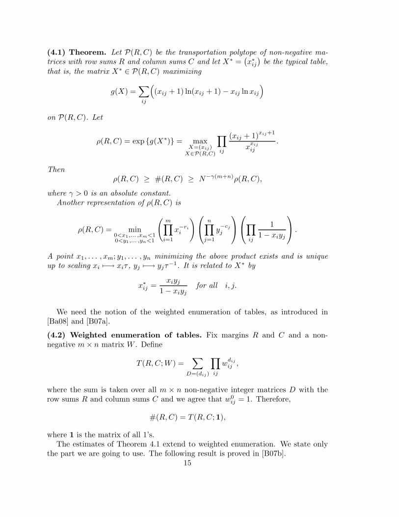
4. Asymptotic estimates
The following result proved in [B07b] provides an asymptotic estimate for thenumber #(R,C) of contingency tables. It explains the role played by the optimiza-tion problem (1.2.1). It will also introduces ingredients needed in the statementand proof of Theorem 5.3 given below.
14
(4.1) Theorem. Let P(R,C) be the transportation polytope of non-negative ma-
trices with row sums R and column sums C and let X∗ =(
x∗ij)
be the typical table,
that is, the matrix X∗ ∈ P(R,C) maximizing
g(X) =∑
ij
(
(xij + 1) ln(xij + 1) − xij lnxij
)
on P(R,C). Let
ρ(R,C) = exp g(X∗) = maxX=(xij)
X∈P(R,C)
∏
ij
(xij + 1)xij+1
xxij
ij
.
Then
ρ(R,C) ≥ #(R,C) ≥ N−γ(m+n)ρ(R,C),
where γ > 0 is an absolute constant.
Another representation of ρ(R,C) is
ρ(R,C) = min0<x1,... ,xm<10<y1,... ,yn<1
(
m∏
i=1
x−ri
i
)
n∏
j=1
y−cj
j
∏
ij
1
1 − xiyj
.
A point x1, . . . , xm; y1, . . . , yn minimizing the above product exists and is unique
up to scaling xi 7−→ xiτ , yj 7−→ yjτ−1. It is related to X∗ by
x∗ij =xiyj
1 − xiyjfor all i, j.
We need the notion of the weighted enumeration of tables, as introduced in[Ba08] and [B07a].
(4.2) Weighted enumeration of tables. Fix margins R and C and a non-negative m× n matrix W . Define
T (R,C;W ) =∑
D=(dij)
∏
ij
wdij
ij ,
where the sum is taken over all m × n non-negative integer matrices D with therow sums R and column sums C and we agree that w0
ij = 1. Therefore,
#(R,C) = T (R,C; 1),
where 1 is the matrix of all 1’s.The estimates of Theorem 4.1 extend to weighted enumeration. We state only
the part we are going to use. The following result is proved in [B07b].15
(4.3) Theorem. Let
ρ(R,C;W ) = infx1,... ,xm>0y1,... ,yn>0
wijxiyj<1 for all i,j
(
m∏
i=1
x−ri
i
)
n∏
j=1
y−cj
j
∏
ij
1
1 − wijxiyj
.
Then
ρ(R,C;W ) ≥ T (R,C;W ) ≥ N−γ(m+n)ρ(R,C;W ),
where γ > 0 is an absolute constant.
In fact, we will only use the upper bound of Theorem 4.3, which is actuallystraightforward to prove since
∏
ij (1 − wijxiyj)−1
is the generating function for
the family T (R,C;W ).
5. The plan of the proofs of Theorems 3.2 and 3.3
To prove Theorems 3.2 and 3.3 we need to understand the behavior of the func-tion
p(X) =NN
N !perB(X),
that is, to estimate values of permanents of doubly stochastic matrices. The follow-ing straightforward corollary of results of [Fa81], [Eg81], [Br73], and [So03] showsthat the permanent of an N × N doubly stochastic matrix lies close to N !/NN
provided the entries of the matrix are not too large. We recall the definition of theGamma function
Γ(t) =
∫ +∞
0
xt−1e−x dx for t > 0.
(5.1) Lemma. Let B = (bij) be an N ×N doubly stochastic matrix and let
zi = maxj=1,... ,N
bij for i = 1, . . . , N.
Suppose thatN∑
i=1
zi ≤ τ for some τ ≥ 1.
Then
N !
NN≤ perB ≤
( τ
N
)N
Γτ
(
1 +N
τ
)
≤ N !
NN(2πN)
τ/2eτ2/12N .
We delay the proof of Lemma 5.1 until Section 7.16
We will apply Lemma 5.1 when τ = O(lnN), in which case the ratio betweenthe upper and lower bounds becomes NO(ln N). In addition, we apply the lemmato the matrix B(X), the doubly stochastic scaling of the random matrix A(X)constructed in Theorem 2.1, see also Section 2.3. However, to use this lemma, weneed to bound the entries of B(X). To do that, we will need to be able to bound theentries of the matrix Y obtained from scaling X to have row sums R and columnsums C. To this end, we prove the following result in Section 8, which might be ofindependent interest.
(5.2) Theorem. Let R = (r1, . . . , rm) and C = (c1, . . . , cn) be positive vectors
such thatm∑
i=1
ri =
n∑
j=1
cj = N.
Let X = (xij) be an m× n positive matrix and let Y = (yij) be the scaling of X to
have row sums R and column sums C, where
yij = λiµjxij for all i, j
and some positive λ1, . . . , λm;µ1, . . . , µn.
Then, for every 1 ≤ p ≤ m and 1 ≤ q ≤ n we have
ln ypq ≤ lnrpcqN
+ lnxpq
+ ln
1
N2
∑
ij
ricjxij
− 1
N
n∑
j=1
cj lnxpj −1
N
m∑
i=1
ri lnxiq.
Now suppose that (R,C) are upper α-smooth margins, that is, ri/N ≤ α/m andcj/N ≤ α/n for some α ≥ 1, fixed in advance. To give an idea of the remainder ofthe argument and the role of the hypotheses, suppose further that xij are sampledindependently at random from the uniform distribution on [0, 1]. Then Theorem 5.2and the law of large numbers clearly imply that asm and n grow, with overwhelmingprobability we have
yij ≤ κricjN
xij for all i, j
and some absolute constant κ > 1. If we construct the doubly stochastic matrixB(X) as in Section 2.3, then with overwhelming probability for the entries bij wewill have
bij ≤ κ
Nfor all i, j.
17
However, in the situation of our proof, the matrix X = (xij) is actually sampledfrom the distribution with density ψ of Section 2.5. Thus to perform a similaranalysis, we need to show that the entries of a random matrix X are uniformlysmall. For that, we have to assume that the margins (R,C) are strongly upperα-smooth (in fact, one can show that merely the condition of upper smoothness isnot enough). Specifically, in Section 9, we prove the following result:
(5.3) Theorem. Let
S ⊂
(i, j) : i = 1, . . . , m; j = 1, . . . , n
be a set of indices, and let X = (xij) be a random m × n matrix with density
ψ = ψR,C of Section 2.5. Suppose that the typical table X∗ =(
x∗ij)
satisfies
x∗ij ≤ λ for all i, j
and some λ > 0.Then for all t > 0 we have
P
∑
(i,j)∈S
xij ≥ t
≤ exp
− t
2λ+ 2
4#SNγ(m+n),
where γ > 0 is the absolute constant of Theorem 4.1.
In Section 10 we complete the proof of Theorem 3.2. Theorem 3.3 requires somemore work and its proof is given in Section 12, after some technical estimates inSection 11.
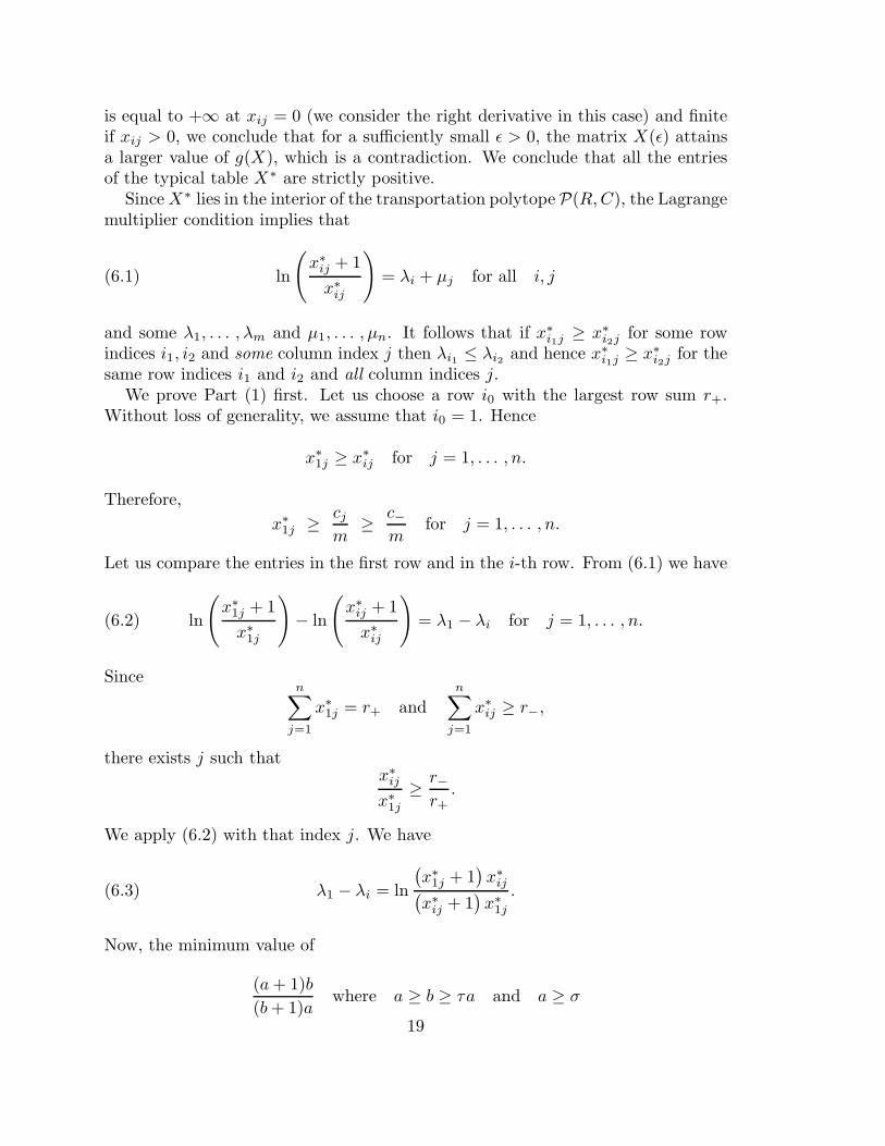
6. Proof of Theorem 3.5
First, we observe that the typical table X∗ =(
x∗ij)
is strictly positive, that is,it lies in the interior of the transportation polytope P(R,C). Indeed, suppose thatx∗11 = 0, for example. Choose indices p and q such that x∗1q > 0 and x∗p1 > 0. Thennecessarily x∗pq < rp, cq and we can consider a perturbation X(ǫ) ∈ P(R,C) of X∗
defined for sufficiently small ǫ > 0 by
xij =
x∗ij + ǫ if i = 1 and j = 1
x∗ij − ǫ if i = p, j = 1 or i = 1, j = q
x∗ij + ǫ if i = p and j = q
x∗ij if i 6= p and j 6= q.
Since the value of∂
∂xijg(X) = ln
(
xij + 1
xij
)
18
is equal to +∞ at xij = 0 (we consider the right derivative in this case) and finiteif xij > 0, we conclude that for a sufficiently small ǫ > 0, the matrix X(ǫ) attainsa larger value of g(X), which is a contradiction. We conclude that all the entriesof the typical table X∗ are strictly positive.
SinceX∗ lies in the interior of the transportation polytope P(R,C), the Lagrangemultiplier condition implies that
(6.1) ln
(
x∗ij + 1
x∗ij
)
= λi + µj for all i, j
and some λ1, . . . , λm and µ1, . . . , µn. It follows that if x∗i1j ≥ x∗i2j for some rowindices i1, i2 and some column index j then λi1 ≤ λi2 and hence x∗i1j ≥ x∗i2j for thesame row indices i1 and i2 and all column indices j.
We prove Part (1) first. Let us choose a row i0 with the largest row sum r+.Without loss of generality, we assume that i0 = 1. Hence
x∗1j ≥ x∗ij for j = 1, . . . , n.
Therefore,
x∗1j ≥ cjm
≥ c−m
for j = 1, . . . , n.
Let us compare the entries in the first row and in the i-th row. From (6.1) we have
(6.2) ln
(
x∗1j + 1
x∗1j
)
− ln
(
x∗ij + 1
x∗ij
)
= λ1 − λi for j = 1, . . . , n.
Sincen∑
j=1
x∗1j = r+ andn∑
j=1
x∗ij ≥ r−,
there exists j such thatx∗ijx∗1j
≥ r−r+.
We apply (6.2) with that index j. We have
(6.3) λ1 − λi = ln
(
x∗1j + 1)
x∗ij(
x∗ij + 1)
x∗1j
.
Now, the minimum value of
(a+ 1)b
(b+ 1)awhere a ≥ b ≥ τa and a ≥ σ
19
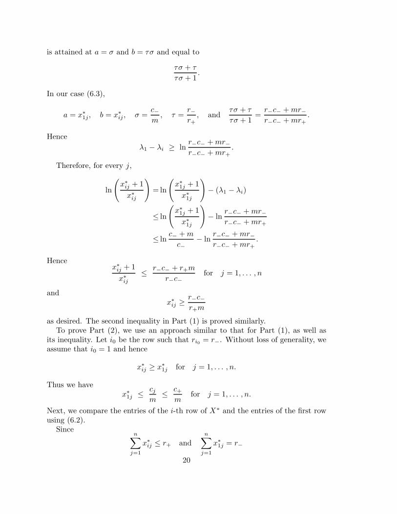
is attained at a = σ and b = τσ and equal to
τσ + τ
τσ + 1.
In our case (6.3),
a = x∗1j, b = x∗ij , σ =c−m, τ =
r−r+, and
τσ + τ
τσ + 1=r−c− +mr−r−c− +mr+
.
Hence
λ1 − λi ≥ lnr−c− +mr−r−c− +mr+
.
Therefore, for every j,
ln
(
x∗ij + 1
x∗ij
)
= ln
(
x∗1j + 1
x∗1j
)
− (λ1 − λi)
≤ ln
(
x∗1j + 1
x∗1j
)
− lnr−c− +mr−r−c− +mr+
≤ lnc− +m
c−− ln
r−c− +mr−r−c− +mr+
.
Hencex∗ij + 1
x∗ij≤ r−c− + r+m
r−c−for j = 1, . . . , n
andx∗ij ≥ r−c−
r+m
as desired. The second inequality in Part (1) is proved similarly.To prove Part (2), we use an approach similar to that for Part (1), as well as
its inequality. Let i0 be the row such that ri0 = r−. Without loss of generality, weassume that i0 = 1 and hence
x∗ij ≥ x∗1j for j = 1, . . . , n.
Thus we havex∗1j ≤ cj
m≤ c+
mfor j = 1, . . . , n.
Next, we compare the entries of the i-th row of X∗ and the entries of the first rowusing (6.2).
Sincen∑
j=1
x∗ij ≤ r+ and
n∑
j=1
x∗1j = r−
20
there is j such thatx∗ijx∗1j
≤ r+r−.
We apply (6.3) with that index j. The maximum value of
(a+ 1)b
(b+ 1)awhere a ≤ b ≤ τa and a ≥ σ
is attained at a = σ, b = τσ and is equal to
τσ + τ
τσ + 1.
In our case of (6.3),
a = x∗1j , b = x∗ij , τ =r+r−, σ =
r−c−r+m
, andτσ + τ
τσ + 1=r−c− +mr+r−c− +mr−
where the expression for σ follows by Part (1). Hence
λ1 − λi ≤ lnr−c− +mr+r−c− +mr−
and for all j we have
ln
(
x∗ij + 1
x∗ij
)
= ln
(
x∗1j + 1
x∗1j
)
− (λ1 − λi)
≥ ln
(
x∗1j + 1
x∗1j
)
− lnr−c− +mr+r−c− +mr−
≥ lnc+ +m
c+− ln
r−c− +mr+r−c− +mr−
.
Hencex∗ij + 1
x∗ij≥ (c+ +m) (r−c− +mr−)
c+ (r−c− +mr+)for j = 1, . . . , n
and the proof follows.
7. Proof of Lemma 5.1
We will use the following bounds for the permanent.21
(7.1) The van der Waerden bound. Let B = (bij) be an N × N doublystochastic matrix, that is,
N∑
j=1
bij = 1 for i = 1, . . . , N and
N∑
i=1
bij = 1 for j = 1, . . . , N
andbij ≥ 0 for i, j = 1, . . . , N.
Then
perB ≥ N !
NN.
This is the famous van der Waerden bound proved by Falikman [Fa81] and Ego-rychev [Eg81], see also Chapter 12 of [LW01] and [G06a].
(7.2) The continuous version of the Bregman-Minc bound. Let B = (bij)be an N ×N matrix such that
N∑
j=1
bij ≤ 1 for i = 1, . . . , N
andbij ≥ 0 i, j = 1, . . . , N.
Furthermore, letzi = max
j=1,... ,Nbij > 0 for i = 1, . . . , N.
Then
perB ≤N∏
i=1
ziΓzi
(
1 + zi
zi
)
.
This bound was obtained by Soules [So03].If zi = 1/ri for integers ri, the bound transforms into
perB ≤N∏
i=1
(ri!)1/ri
ri,
which can be easily deduced from the Minc conjecture proved by Bregman, see[Br73].
Now we are ready to prove Lemma 5.1.
Proof of Lemma 5.1. The lower bound is the van der Waerden bound.To prove the upper bound, define
f(ξ) = ξ ln Γ
(
1 + ξ
ξ
)
+ ln ξ for 0 < ξ ≤ 1.
22
Then f is a concave function and by the Bregman-Minc bound, we have
ln perB ≤N∑
i=1
f(zi).
The function
F (x) =
N∑
i=1
f(ξi) for x = (ξ1, . . . , ξN )
is concave on the simplex defined by the equation ξ1 + . . .+ξN = τ and inequalitiesξi ≥ 0 for i = 1, . . . , N . It is also symmetric under permutations of ξ1, . . . , ξN .Hence the maximum of F is attained at
ξ1 = . . . = ξN = τ/N,
and soln perB ≤ Nf
( τ
N
)
.
Thus
perB ≤( τ
N
)N
Γτ
(
1 +N
τ
)
and the rest follows by Stirling’s formula.
8. Proof of Theorem 5.2
We begin our proof by restating a theorem of Bregman [Br73] in a slightly moregeneral form.
(8.1) Theorem. Let Y = (yij) be the positive m× n matrix that is the scaling of
a positive m× n matrix X = (xij) to have margins (R,C). Then
∑
ij
yij (ln yij − lnxij) ≤∑
ij
zij (ln zij − lnxij)
for every matrix Z ∈ P(R,C), where P(R,C) is the transportation polytope of
m× n non-negative matrices with row sums R and column sums C.
Proof. The function
f(Z) =∑
ij
zij (ln zij − lnxij)
is strictly convex on P(R,C) and hence attains its unique minimum Y ′ =(
y′ij)
on P(R,C). As in the proof of Theorem 3.5 (see Section 6), we can show that Y ′
is strictly positive, that is, Y ′ lies in the relative interior of P(R,C). Writing theLagrange multiplier conditions, we obtain
ln y′ij − lnxij = ξi + ηj
23
for some ξ1, . . . , ξm and η1, . . . , ηn. Letting λi = eξi and µj = eηj we obtain
y′ij = λiµjxij for all i, j,
so in fact Y ′ = Y as desired.
Next, we prove a lemma that extends a result of Linial, Samorodnitsky, andWigderson [L+00].
(8.2) Lemma. Let R = (r1, . . . , rm) and C = (c1, . . . , cn) be positive vectors such
thatm∑
i=1
ri =
n∑
j=1
cj = N.
Let X = (xij) be an m× n positive matrix such that
∑
ij
xij = N
and let Y = (yij) be the scaling of X to have row sums R and column sums C.
Then∑
ij
ricj ln yij ≥∑
ij
ricj lnxij .
Proof. Since Y is the limit of the sequence of matrices obtained from X by repeatedalternate scaling of the rows to have row sums r1, . . . , rm and of the columns tohave column sums c1, . . . , cn, cf., for example, Chapter 6 of [BR97], it suffices toshow that when the rows (columns) are scaled, the corresponding weighted sumsof the logarithms of the entries of the matrix can only increase.
To this end, let X = (xij) be a positive m × n matrix with the row sumsσ1, . . . , σm such that
m∑
i=1
σi = N
and let Y = (yij) be the matrix obtained from Y by scaling the rows to have sumsr1, . . . , rm. Hence,
yij = rixij/σi for all i, j.
Thus∑
ij
ricj (ln yij − lnxij) =n∑
j=1
cj
(
m∑
i=1
(ri ln ri − ri lnσi)
)
≥ 0,
since the maximum of the function
m∑
i=1
ri ln ξi
24
on the simplex
m∑
i=1
ξi = N and ξi ≥ 0 for i = 1, . . . , m
is attained at ξi = ri.
The scaling of columns is treated similarly.
Proof of Theorem 5.2. Without loss of generality, we assume that p = q = 1.
Define an m× n matrix U = (uij) by
(8.3) uij =ricjxij
Tfor T =
1
N
∑
ij
ricjxij .
We note that the scalings of U and X to margins (R,C) coincide and that
∑
ij
uij = N.
By Theorem 8.1, the matrix Y minimizes
∑
ij
zij (ln zij − lnuij) ,
over the set P(R,C) of m × n non-negative matrices Z with row sums R and thecolumn sums C.
For a real t, let us define the matrix Y (t) = (yij(t)) by
yij(t) =
yij + t if i = j = 1
yij − cj
N−c1t if i = 1, j 6= 1
yij − ri
N−r1t if i 6= 1, j = 1
yij +ricj
(N−r1)(N−c1)t if i 6= 1, j 6= 1.
Then Y (0) = Y and Y (t) ∈ P(R,C) for all t sufficiently close to 0. Therefore,
d
dtf (Y (t))
∣
∣
t=0= 0,
where
f(Z) =∑
ij
zij (ln zij − lnuij) .
25
Therefore,
ln y11 − lnu11 + 1
− 1
N − c1
∑
j 6=1
cj (ln y1j − lnu1j + 1)
− 1
N − r1
∑
i6=1
ri (ln yi1 − lnui1 + 1)
+1
(N − r1)(N − c1)
∑
i,j 6=1
ricj (ln yij − lnuij + 1)
= 0.
Rearranging the summands,
N2
(N − r1)(N − c1)(ln y11 − lnu11)
− N
(N − r1)(N − c1)
n∑
j=1
cj (ln y1j − lnu1j)
− N
(N − r1)(N − c1)
m∑
i=1
ri (ln yi1 − lnui1)
+1
(N − r1)(N − c1)
∑
ij
ricj (ln yij − lnuij)
= 0.
On the other hand, by Lemma 8.2,
∑
ij
ricj (ln yij − lnuij) ≥ 0,
so we must have
N2 (ln y11 − lnu11) −N
n∑
j=1
cj (ln y1j − lnu1j) −N
m∑
i=1
ri (ln yi1 − lnui1) ≤ 0.
In other words,
ln y11 ≤ lnu11 +1
N
n∑
j=1
cj (ln y1j − lnu1j) +1
N
m∑
i=1
ri (ln yi1 − lnui1) .
Sincen∑
j=1
y1j = r1,
26
we haven∑
j=1
cj ln y1j ≤n∑
j=1
cj ln(cjr1N
)
,
cf. the proof of Lemma 8.2. Similarly, since
m∑
i=1
yi1 = c1,
we havem∑
i=1
ri ln yi1 ≤m∑
i=1
ri ln(ric1N
)
.
Substituting (8.3) for U , we obtain
ln y11 ≤ lnx11 + ln (r1c1) − lnT +1
N
n∑
j=1
cj lnT
Nx1j+
1
N
m∑
i=1
ri lnT
Nxi1,
and the proof follows.
9. Proof of Theorem 5.3
Fix margins (R,C), let ψ = ψR,C be the density of Section 2.5, and let X = (xij)be the random matrix distributed in accordance with the density ψ. We will needa lemma that connects linear functionals of X with the weighted sums T (R,C;W )of Section 4.2.
(9.1) Lemma. Let λij < 1 be real numbers.
(1) Let W = (wij) be the m× n matrix of weights given by
wij = (1 − λij)−1
for all i, j.
Then
E exp
∑
ij
λijxij
=T (R,C;W )
#(R,C)
∏
ij
wij ;
(2) We have
E∏
ij
x−λij
ij =1
#(R,C)
∑
D=(dij)
∏
ij
Γ (dij − λij + 1)
Γ (dij + 1),
where the sum is taken over all m × n non-negative integer matrices D =(dij) with row sums R and column sums C.
27
Proof. Let us prove Part (1). We have
E exp
∑
ij
λijxij
=1
#(R,C)
∫
Rmn+
exp
−∑
ij
(1 − λij) xij
×∑
D=(dij)
∏
ij
xdij
ij
dij !dX
=1
#(R,C)
∫
Rmn+
exp
−∑
ij
xij
×∑
D=(dij)
∏
ij
wdij
ij xdij
ij
dij !
∏
ij
wij dX
=T (R,C;W )
#(R,C)
∏
ij
wij ,
as desired.Since
ψ(X)∏
ij
x−λij
ij =1
#(R,C)
∑
D=(dij)
∏
ij
xdij−λij
ij
dij !e−xij ,
the proof of Part (2) follows.
To prove Theorem 5.3 we need only Part (1) of the lemma, while Part (2) willbe used later in the proof of Theorem 3.3.
Proof of Theorem 5.3. We use the Laplace transform method, see, for example,Appendix A of [AS92]. We have
P
∑
(i,j)∈S
xij ≥ t
=P
exp
1
2λ+ 2
∑
(i,j)∈S
xij
≥ exp
t
2λ+ 2
≤ exp
− t
2λ+ 2
E exp
1
2λ+ 2
∑
(i,j)∈S
xij
,
by the Markov inequality.By Part (1) of Lemma 9.1,
E exp
1
2λ+ 2
∑
(i,j)∈S
xij
=T (R,C;W )
#(R,C)
(
2λ+ 2
2λ+ 1
)#S
,
28
where
wij =
(2λ+ 2)/(2λ+ 1) if (i, j) ∈ S
1 if (i, j) /∈ S.
Clearly,(
2λ+ 2
2λ+ 1
)#S
≤ 2#S .
To bound the ratio of T (R,C;W ) and #(R,C), we use Theorems 4.1 and 4.3.Let 0 < x1, . . . , xm; y1, . . . , yn < 1 be numbers such that
ρ(R,C) =
(
m∏
i=1
xi−ri
)
n∏
j=1
yj−cj
∏
ij
1
1 − xiyj
.
For the typical table X∗ =(
x∗ij)
we have
x∗ij =xiyj
1 − xiyj≤ λ for all i, j.
Therefore,
xiyj =x∗ij
1 + x∗ij≤ λ
λ+ 1for all i, j
andwijxiyj < 1 for all i, j.
Then we have
ρ(R,C;W ) ≤(
m∏
i=1
xi−ri
)
n∏
j=1
yj−cj
∏
ij
1
1 − wijxiyj
andρ(R,C;W )
ρ(R,C)≤
∏
(i,j)∈S
1 − xiyj
1 − wijxiyj=
∏
(i,j)∈S
1
1 + (1 − wij)x∗ij
.
Now1
1 + (1 − wij)x∗ij≤ 2λ+ 1
λ+ 1≤ 2 for all (i, j) ∈ S
and henceρ(R,C;W )
ρ(R,C)≤ 2#S .
Since
T (R,C;W ) ≤ ρ(R,C;W ) and #(R,C) ≥ ρ(R,C)N−γ(m+n),
the proof follows.
We will need the following corollary.29
(9.2) Corollary. Suppose that m ≥ n and that the typical table X∗ =(
x∗ij)
satisfies
x∗ij ≤ λ for all i, j
and some λ > 0. Let X = (xij) be a random m×n matrix distributed in accordance
with the density ψR,C , and let
ui = maxj=1,... ,n
xij .
Then for some τ = τ(λ) > 0 we have
P
m∑
i=1
ui ≥ (λ+ 1)τm lnN
≤ 4−m.
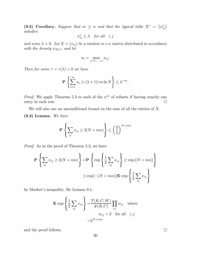
Proof. We apply Theorem 5.3 to each of the nm of subsets S having exactly oneentry in each row.
We will also use an unconditional bound on the sum of all the entries of X .
(9.3) Lemma. We have
P
∑
ij
xij ≥ 2(N +mn)
≤(
3
4
)N+mn
Proof. As in the proof of Theorem 5.3, we have
P
∑
ij
xij ≥ 2(N +mn)
=P
exp
1
2
∑
ij
xij
≥ exp N +mn
≤ exp−(N +mn)E exp
1
2
∑
ij
xij
by Markov’s inequality. By Lemma 9.1,
E exp
1
2
∑
ij
xij
=T (R,C;W )
#(R,C)
∏
ij
wij where
wij = 2 for all i, j
=2N+mn
and the proof follows.
30
10. Proof of Theorem 3.2
We start with a technical result.
(10.1) Lemma. Let (R,C) be upper α-smooth margins, so ri/N ≤ α/m and
cj/N ≤ α/n for all i, j. Let X = (xij) be a random m × n matrix with density
ψR,C of Section 2.5. Then for any real τ
P
1
N
n∑
j=1
cj lnxij ≤ −τ
≤ 2n exp
−nτ2α
and
P
1
N
m∑
i=1
ri lnxij ≤ −τ
≤ 2m exp
−mτ2α
.
Proof. Let us prove the first inequality. As in the proof of Theorem 5.3, we use theLaplace transform method. We have
P
1
N
n∑
j=1
cj lnxij ≤ −τ
=P
− n
2αN
n∑
j=1
cj lnxij ≥ nτ
2α
≤ exp
−nτ2α
E exp
− n
2αN
n∑
j=1
cj lnxij
= exp
−nτ2α
En∏
j=1
x−λj
ij where λj =ncj2αN
.
Since
λj ≤ 1
2,
by Part (2) of Lemma 9.1 we deduce that
E
n∏
j=1
x−λj
ij ≤(
Γ
(
1
2
))n
≤ 2n
(we observe that every term in the sum of Lemma 9.1 does not exceed Γn(1/2)).The proof of the second inequality is identical.
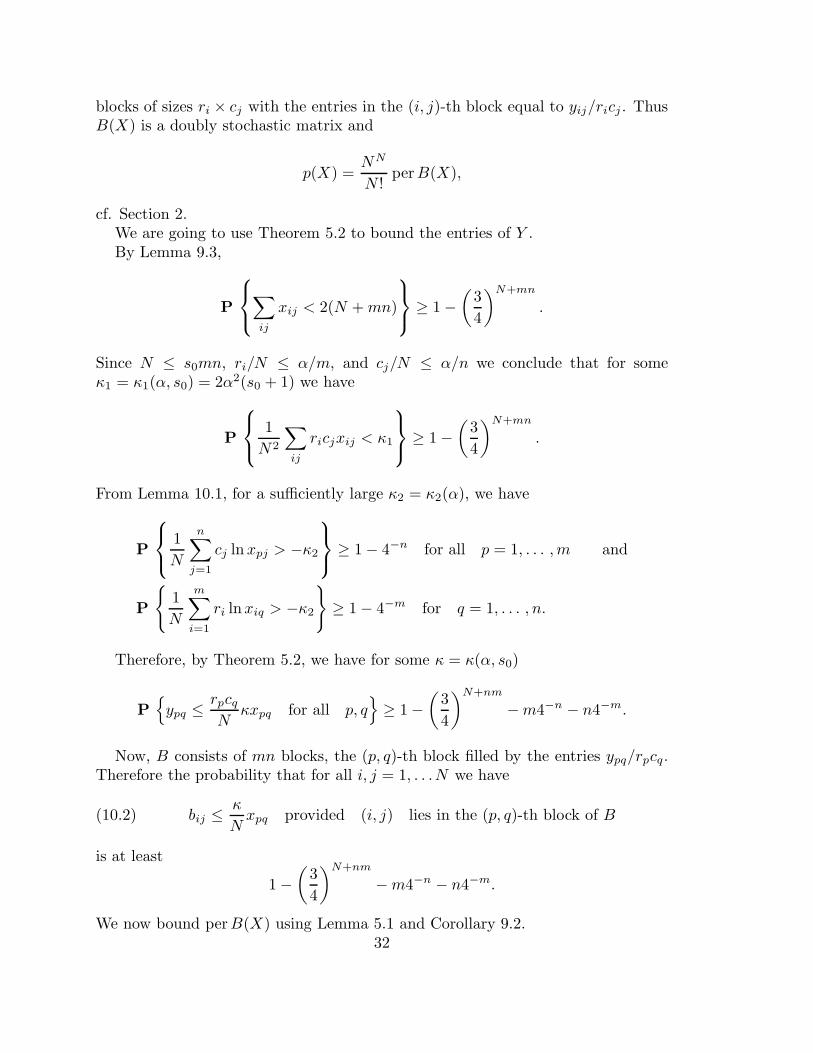
Proof of Theorem 3.2. Without loss of generality, we assume that m ≥ n. Werecall that function p(X) is computed as follows. Given a positive m × n matrixX = (xij), we compute the scaling Y = (yij) of X to have row sums R and thecolumn sums C. Then we compute the N ×N block matrix B(X) consisting of mn
31
blocks of sizes ri × cj with the entries in the (i, j)-th block equal to yij/ricj . ThusB(X) is a doubly stochastic matrix and
p(X) =NN
N !perB(X),
cf. Section 2.We are going to use Theorem 5.2 to bound the entries of Y .By Lemma 9.3,
P
∑
ij
xij < 2(N +mn)
≥ 1 −(
3
4
)N+mn
.
Since N ≤ s0mn, ri/N ≤ α/m, and cj/N ≤ α/n we conclude that for someκ1 = κ1(α, s0) = 2α2(s0 + 1) we have
P
1
N2
∑
ij
ricjxij < κ1
≥ 1 −(
3
4
)N+mn
.
From Lemma 10.1, for a sufficiently large κ2 = κ2(α), we have
P
1
N
n∑
j=1
cj lnxpj > −κ2
≥ 1 − 4−n for all p = 1, . . . , m and
P
1
N
m∑
i=1
ri lnxiq > −κ2
≥ 1 − 4−m for q = 1, . . . , n.
Therefore, by Theorem 5.2, we have for some κ = κ(α, s0)
P
ypq ≤ rpcqN
κxpq for all p, q
≥ 1 −(
3
4
)N+nm
−m4−n − n4−m.
Now, B consists of mn blocks, the (p, q)-th block filled by the entries ypq/rpcq.Therefore the probability that for all i, j = 1, . . .N we have
(10.2) bij ≤ κ
Nxpq provided (i, j) lies in the (p, q)-th block of B
is at least
1 −(
3
4
)N+nm
−m4−n − n4−m.
We now bound perB(X) using Lemma 5.1 and Corollary 9.2.32
Let
zi = maxj=1,... ,N
bij for i = 1, . . .N and let
up = maxq=1,... ,m
xpq.
Then, from (10.2) we have
N∑
i=1
zi ≤κ
N
m∑
p=1
rpup ≤ ακ
m
m∑
p=1
up.
By Corollary 9.2, for some τ1 = τ1(α, s0), we have
P
m∑
p=1
um ≤ τ1m lnN
≥ 1 − 4−m.
Thus for some τ = τ(α, s0) we have
P
N∑
i=1
zi ≤ τ lnN
≥ 1 −(
3
4
)N+mn
−m4−n − n4−m − 4−m
and the proof follows by Lemma 5.1.
The rest of the paper deals with the proof of Theorem 3.3. This requires sharp-ening of the estimates of Lemma 10.1. Roughly, we need to prove that with over-whelming probability
1
N
n∑
j=1
cj lnxij ≥ −τ + ln s and
1
N
m∑
i=1
ri lnxij ≥ −τ + ln s
for some constant τ = τ(α, β), where s = N/mn is the average entry of the table.
11. An estimate of a sum over tables
To sharpen the estimates of Lemma 10.1 we need a more careful estimate of thesum in Part (2) of Lemma 9.1. In this section, we prove the following technicalresult.
33
(11.1) Proposition. Suppose that (R,C) are lower β-smooth and upper α-smooth
margins and that
s = N/mn ≥ 1.
Let λ1, . . . , λm ≤ 1/2 be numbers and let l = λ1 + . . . + λm. Then, for k < n we
have1
#(R,C)
∑
D=(dij)
∏
1≤i≤m1≤j≤k
Γ(dij − λi + 1)
Γ(dij + 1)≤ δkmNγ(m+n)s−kl,
where the sum is taken over all non-negative integer matrices D with row sums Rand column sums C, δ = δ(α, β) > 0 and γ is the absolute constant of Theorem
4.1.
We start with computing a simplified version of this sum in a closed form.
(11.2) Definition. Let us fix positive integers c and m. The integer simplex
Υ(m, c) is the set of all non-negative integer vectors a = (d1, . . . , dm) such thatd1 + . . .+ dm = c.
Clearly,
#Υ(m, c) =
(
m+ c− 1
m− 1
)
.
A sum over Υ(m, c) similar to that of Proposition 11.1 can be computed in aclosed form.
(11.3) Lemma. Let λi < 1, i = 1, . . . , m, be numbers and let l = λ1 + . . .+ λm.
Then
1
#Υ(m, c)
∑
d1,... ,dm≥0d1+...+dm=c
m∏
i=1
Γ (di − λi + 1)
Γ (di + 1)=
Γ(c+m− l)Γ(m)
Γ(c+m)Γ(m− l)
m∏
i=1
Γ (1 − λi) .
Proof. Let us define a function hc on the positive orthant Rm+ by the formula
hc(x) =(m− 1)!
(m+ c− 1)!
(
m∑
i=1
ξi
)c
exp
−m∑
i=1
ξi
for x = (ξ1, . . . , ξm) ∈ Rm+ .
Since(
m∑
i=1
ξi
)c
=∑
d1,... ,dm≥0d1+...+dm=c
c!
d1! · · ·dm!ξd1
1 · · · ξdmm ,
We can rewrite
hc(x) =
(
m+ c− 1
m− 1
)−1∑
d1,... ,dm≥0d1+...+dm=c
m∏
i=1
ξdi
i
di!e−ξi .
34
Therefore,
1
#Υ(m, c)
∑
d1,... ,dm≥0d1+...+dm=c
m∏
i=1
Γ (di − λi + 1)
Γ (di + 1)=
∫
Rm+
hc(x)
m∏
i=1
ξ−λi
i dx.
Let Q ⊂ Rm+ be the simplex ξ1 + . . . + ξm = 1 with the Lebesgue measure dx
normalized to the probability measure. Since the function
(
m∑
i=1
ξi
)c m∏
i=1
ξ−λi
i
is positive homogeneous of degree c− l, we can write
(11.3.1)
∫
Rm+
hc(x)m∏
i=1
ξ−λi
i dx =Γ(c+m− l)
Γ(m)
∫
Q
hc(x)m∏
i=1
ξ−λi
i dx
On the other hand,
(11.3.2) hc(x) =Γ(m)
Γ(c+m)h0(x) for x ∈ Q.
Using (11.3.1) with c = 0, we deduce that
∫
Q
h0(x)
m∏
i=1
ξ−λi
i dx =Γ(m)
Γ(m− l)
∫
Rm+
h0(x)
m∏
i=1
ξ−λi
i dx
=Γ(m)
Γ(m− l)
m∏
i=1
∫ +∞
0
ξ−λi
i e−ξi dξi
=Γ(m)
Γ(m− l)
m∏
i=1
Γ (1 − λi) .
Now, from (11.3.1) and (11.3.2), we have
∫
Rm+
hc(x)m∏
i=1
ξ−λi
i dx =Γ(c+m− l)Γ(m)
Γ(c+m)Γ(m− l)
m∏
i=1
Γ (1 − λi) ,
as desired.
We need an estimate.35
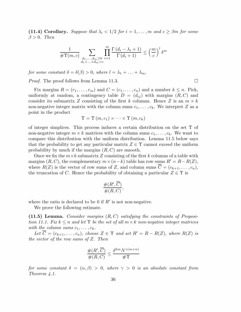
(11.4) Corollary. Suppose that λi < 1/2 for i = 1, . . . , m and c ≥ βm for some
β > 0. Then
1
#Υ(m, c)
∑
d1,... ,dm≥0d1+...+dm=c
m∏
i=1
Γ (di − λi + 1)
Γ (di + 1)≤(m
c
)l
δm
for some constant δ = δ(β) > 0, where l = λ1 + . . .+ λm.
Proof. The proof follows from Lemma 11.3.
Fix margins R = (r1, . . . , rm) and C = (c1, . . . , cn) and a number k ≤ n. Pick,uniformly at random, a contingency table D = (dij) with margins (R,C) andconsider its submatrix Z consisting of the first k columns. Hence Z is an m × knon-negative integer matrix with the column sums c1, . . . , ck. We interpret Z as apoint in the product
Υ = Υ(m, c1) × · · · × Υ(m, ck)
of integer simplices. This process induces a certain distribution on the set Υ ofnon-negative integer m× k matrices with the column sums c1, . . . , ck. We want tocompare this distribution with the uniform distribution. Lemma 11.5 below saysthat the probability to get any particular matrix Z ∈ Υ cannot exceed the uniformprobability by much if the margins (R,C) are smooth.
Once we fix them×k submatrix Z consisting of the first k columns of a table withmargins (R,C), the complementary m×(n−k) table has row sums R′ = R−R(Z),where R(Z) is the vector of row sums of Z, and column sums C = (ck+1, . . . , cn),the truncation of C. Hence the probability of obtaining a particular Z ∈ Υ is
#(R′, C)
#(R,C),
where the ratio is declared to be 0 if R′ is not non-negative.We prove the following estimate.
(11.5) Lemma. Consider margins (R,C) satisfying the constraints of Proposi-
tion 11.1. Fix k ≤ n and let Υ be the set of all m×k non-negative integer matrices
with the column sums c1, . . . , ck.Let C = (ck+1, . . . , cn), choose Z ∈ Υ and set R′ = R − R(Z), where R(Z) is
the vector of the row sums of Z. Then
#(R′, C)
#(R,C)≤ δkmNγ(m+n)
#Υ
for some constant δ = (α, β) > 0, where γ > 0 is an absolute constant from
Theorem 4.1.
36
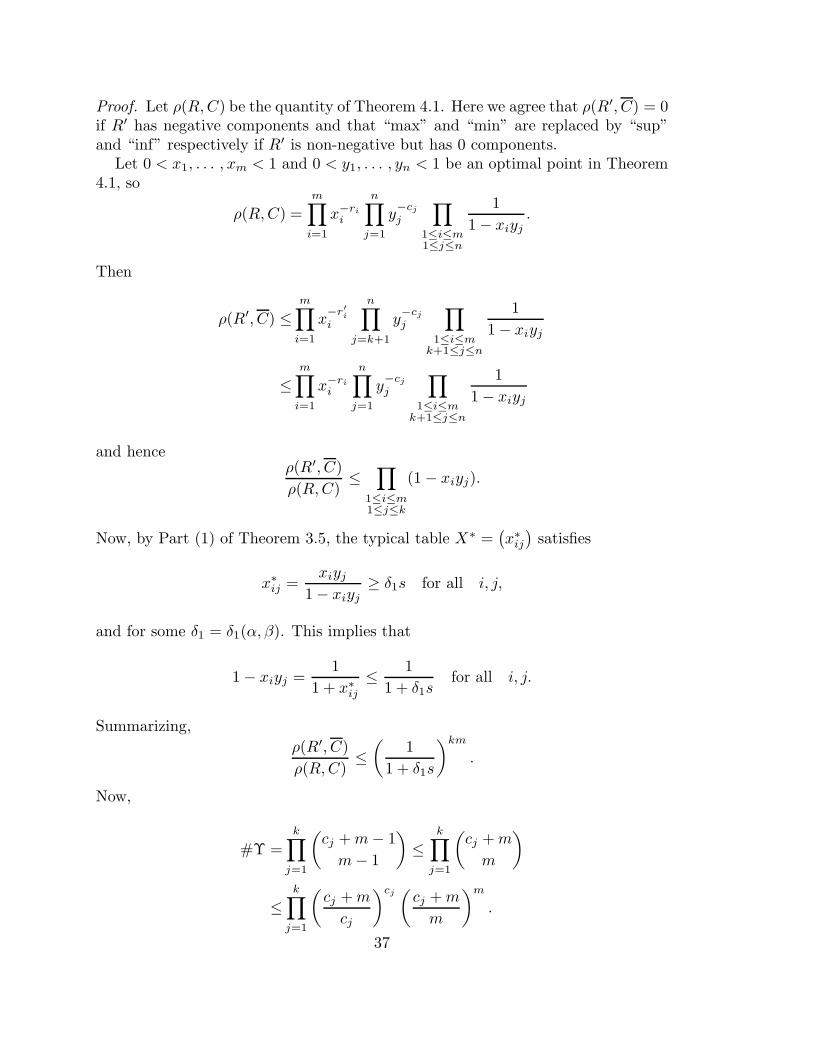
Proof. Let ρ(R,C) be the quantity of Theorem 4.1. Here we agree that ρ(R′, C) = 0if R′ has negative components and that “max” and “min” are replaced by “sup”and “inf” respectively if R′ is non-negative but has 0 components.
Let 0 < x1, . . . , xm < 1 and 0 < y1, . . . , yn < 1 be an optimal point in Theorem4.1, so
ρ(R,C) =m∏
i=1
x−ri
i
n∏
j=1
y−cj
j
∏
1≤i≤m1≤j≤n
1
1 − xiyj.
Then
ρ(R′, C) ≤m∏
i=1
x−r′
i
i
n∏
j=k+1
y−cj
j
∏
1≤i≤mk+1≤j≤n
1
1 − xiyj
≤m∏
i=1
x−ri
i
n∏
j=1
y−cj
j
∏
1≤i≤mk+1≤j≤n
1
1 − xiyj
and henceρ(R′, C)
ρ(R,C)≤
∏
1≤i≤m1≤j≤k
(1 − xiyj).
Now, by Part (1) of Theorem 3.5, the typical table X∗ =(
x∗ij)
satisfies
x∗ij =xiyj
1 − xiyj≥ δ1s for all i, j,
and for some δ1 = δ1(α, β). This implies that
1 − xiyj =1
1 + x∗ij≤ 1
1 + δ1sfor all i, j.
Summarizing,
ρ(R′, C)
ρ(R,C)≤(
1
1 + δ1s
)km
.
Now,
#Υ =
k∏
j=1
(
cj +m− 1
m− 1
)
≤k∏
j=1
(
cj +m
m
)
≤k∏
j=1
(
cj +m
cj
)cj(
cj +m
m
)m
.
37
We have(
cj +m
cj
)cj
≤ em.
Furthermore, since cj ≤ αsm, we have(
cj +m
m
)m
≤ (1 + αs)m
and
#Υρ(R′, C)
ρ(R,C)≤ ekm
(
1 + αs
1 + δ1s
)km
≤ δkm.
Since by Theorem 4.1 we have
#(R,C) ≥ N−γ(m+n)ρ(R,C) and #(R′, C) ≤ ρ(R′, C),
the proof follows.
Proof of Proposition 11.1. Let Υ(m, cj) be the integer simplex of non-negativeinteger vectors summing up to cj and let
Υ = Υ(m, c1) × · · · × Υ(m, ck).
Using Lemma 11.5, we bound
1
#(R,C)
∑
D=(dij)
∏
1≤i≤m1≤j≤k
Γ(dij − λi + 1)
Γ(dij + 1)
=∑
Z=(zij)Z∈Υ
#(R−R(Z), C)
#(R,C)
∏
1≤i≤m1≤j≤k
Γ(zij − λi + 1)
Γ(zij + 1)
≤δkm1 Nγ(m+n)
#Υ
∑
Z=(zij)Z∈Υ
∏
1≤i≤m1≤j≤k
Γ(zij − λi + 1)
Γ(zij + 1)
for some δ1 = δ(α, β). The sum
1
#Υ
∑
Z=(zij)Z∈Υ
∏
1≤i≤m1≤j≤k
Γ(zij − λi + 1)
Γ(zij + 1)
is just the product of k sums of the type
1
Υ(m, cj)
∑
d1,... ,dm≥0d1+...+dm=cj
m∏
i=1
Γ(di − λi + 1)
Γ(di + 1)≤(
m
cj
)l
δm2
by Corollary 11.4, for some δ2 = δ(α, β). The proof now follows.
38
12. Proof of Theorem 3.3
Fix margins (R,C) and let X = (xij) be the m× n random matrix with densityψ = ψR,C of Section 2.5. Define random variables
hi =1
N
n∑
j=1
cj lnxij for i = 1, . . . , m and
vj =1
N
m∑
i=1
ri lnxij for j = 1, . . . , n.
(12.1) Lemma. Let (R,C) be lower β-smooth upper α-smooth margins such that
s = N/mn ≥ 1.Choose a subset J ⊂ 1, . . . , n of indices, #J = k. Then for all t > 0 we have
P
1
k
∑
j∈J
vj ≤ −t+ ln s
≤ exp
− tkm2α
δkmNγ(m+n),
Similarly, for a subset I ⊂ 1, . . . , m of indices, #I = k, we have
P
1
k
∑
i∈I
hi ≤ −t+ ln s
≤ exp
− tkn2α
δknNγ(m+n).
for some number δ = δ(α, β) > 0 and the absolute constant γ > 0 of Theorem 4.1.
Proof. Without loss of generality, it suffices to prove only the first bound and onlyin the case of J = 1, . . . , k.
We use the Laplace transform method. We have
P
1
k
k∑
j=1
vj ≤ −t+ ln s
=P
−m
2α
k∑
j=1
vj ≥ tkm
2α− km ln s
2α
=P
exp
−m
2α
k∑
j=1
vj
≥ s−km2α · exp
tkm
2α
≤s km2α exp
− tkm2α
·E exp
−m
2α
k∑
j=1
vj
.
Let
λi =mri2αN
≤ 1
2for i = 1, . . . , m and
l = λ1 + . . .+ λm =m
2α.
39
Using Part (2) of Lemma 9.1, we write
E exp
−m
2α
k∑
j=1
vj
=1
#(R,C)
∑
D=(dij)
∏
1≤i≤m1≤j≤k
Γ(dij − λi + 1)
Γ(dij + 1),
where the sum is taken over all contingency tables D with margins (R,C).The proof now follows by Proposition 11.1.
We will use the following corollary.
(12.2) Corollary. Let (R,C) be lower β-smooth upper α-smooth margins such that
s = N/mn ≥ 1. Suppose further that m ≤ ρn and n ≤ ρm for some ρ ≥ 1.Then
for some τ = τ(α, β, ρ) > 0 we have
P
#
i : hi ≤ −τ + ln s
> lnN
≤ 4−n and
P
#
j : vj ≤ −τ + ln s
> lnN
≤ 4−m.
Proof. We introduce random sets
I =
i : hi ≤ −τ + ln s
and J =
j : vj ≤ −τ + ln s
and note that
1
#I
∑
i∈I
hi ≤ −τ + ln s and1
#J
∑
j∈J
vj ≤ −τ + ln s.
The proof now follows from Lemma 12.1.
Proof of Theorem 3.3. The proof is a modification of that of Theorem 3.2. Werecall that
p(X) =NN
N !perB(X),
where B(X) is the N × N doubly stochastic matrix constructed as follows: wescale m × n matrix X to the matrix Y with row sums R and column sums C andlet bij = ypq/rpcq provided the entry (i, j) lies in the (p, q)-th block B(X) of sizerp × cq. We are going to bound the entries of Y . First, without loss of generalitywe assume that s = N/mn ≥ 1 since the case of s ≤ 1 is treated in Theorem 3.2.
As in the proof of Theorem 3.2 we conclude that
(12.3) P
1
N2
∑
ij
ricjxij < 2α2(s+ 1)
≥ 1 −(
3
4
)N+mn
.
40
Let
hp =1
N
N∑
j=1
cj lnxpj for p = 1, . . . , m and
vq =1
N
m∑
i=1
ri lnxiq for q = 1, . . . , n.
Choose τ > 0 as in Corollary 12.2. Set
P =
p : hp ≤ −τ + ln s
and Q =
q : vq ≤ −τ + ln s
.
Thus the probability that
#P ≤ lnN and #Q ≤ lnN
is at least1 − 4−m − 4−n.
If p /∈ P and q /∈ Q and (12.3) holds then by Theorem 5.2,
ypq ≤ δ1rpcqsN
xpq
for some δ1(α, β) > 0. If p ∈ P or q ∈ Q then
ypq ≤ minrp, cq.
Consequently, for bij with (i, j) in the p, q-th block we have
bij ≤ δ1sN
xpq if p /∈ P and q /∈ Q
and
bij ≤ min
1
rp,
1
cq
if p ∈ P or q ∈ Q.
As in the proof of Theorem 3.2, we let
zi = maxj=1,... ,N
bij for i = 1, . . .N and let
up = maxq=1,... ,m
xpq.
We estimate that
zi ≤1
rp41
if i lies in the p-th row block with p ∈ P and we estimate that
zi ≤δ1sN
up + maxq∈Q
ypq
rpcq,
if i lies in the row block p /∈ P . Hence
N∑
i=1
zi ≤ #P +δ1sN
m∑
p=1
rpup +m∑
p=1
maxq∈Q
ypq
cq.
By Corollary 9.2,
P
m∑
p=1
up ≥ τ1sm lnN
≤ 4−m
for some τ1 = τ1(α), and hence
P
δ1sN
m∑
p=1
rpup ≤ δ2 lnN
≥ 1 − 4−m.
for some δ2 = δ2(α). Finally,
m∑
p=1
maxq∈Q
ypq
cq≤∑
q∈Q
m∑
p=1
ypq
cq≤ δ3#Q
for some δ3 = δ3(α, β). Summarizing,
P
N∑
i=1
zi ≤ δ lnN
≥ 1 −(
3
4
)N+mn
− 4−n − 2 · 4−m
for some δ = δ(α, β, ρ) > 0 and the proof is completed as in Theorem 3.2.
Acknowledgments
The authors are grateful to Jesus De Loera who computed some of the valuesof #(R,C) for us using his LattE code. The fourth author would like to thankRadford Neal and Ofer Zeitouni for helpful discussions.
The research of the first author was partially supported by NSF Grant DMS0400617. The research of the third author was partially supported by ISF grant039-7165. The research of the first and third authors was also partially supported bya United States - Israel BSF grant 2006377. The research of the fourth author waspartially completed while he was an NSF sponsored visitor at the Institute for Pureand Applied Mathematics at UCLA, during April-June 2006. The fourth authorwas also partially supported by NSF grant 0601010 and an NSERC Postdoctoralfellowship held at the Fields Institute, Toronto.
42
References
[AS92] N. Alon and J.H. Spencer, The Probabilistic Method. With an Appendix by Paul Erdos,Wiley-Interscience Series in Discrete Mathematics and Optimization, John Wiley & Sons,
Inc., New York, 1992.
[AK91] D. Applegate and R. Kannan, Sampling and integration of near log-concave functions,
Proceedings of the Twenty-Third Annual ACM Symposium on Theory of Computing,ACM, New York, NY, 1991, pp. 156–163.
[B+04] W. Baldoni-Silva, J.A. De Loera, and M. Vergne, Counting integer flows in networks,
Found. Comput. Math. 4 (2004), 277–314.
[BR97] R.B. Bapat and T.E.S. Raghavan, Nonnegative Matrices and Applications, Encyclopedia
of Mathematics and its Applications, vol. 64, Cambridge University Press, Cambridge,1997.
[B07a] A. Barvinok, Brunn-Minkowski inequalities for contingency tables and integer flows,Advances in Mathematics 211 (2007), 105–122.
[B07b] A. Barvinok, Asymptotic estimates for the number of contingency tables, integer flows,
and volumes of transportation polytopes, preprint arXiv:0709.3810 (2007).
[Ba08] A. Barvinok, Enumerating contingency tables via random permanents, Combinatorics,
Probability and Computing 17 (2008), 1-19.
[B+07] A. Barvinok, A. Samorodnitsky, and A. Yong, Counting magic squares in quasi-polynomial time, preprint arXiv:math/0703227 (2008).
[B+72] A. Bekessy, P. Bekessy, and J. Komlos, Asymptotic enumeration of regular matrices,Studia Sci. Math. Hungar. 7 (1972), 343–353.
[Br73] L.M. Bregman, Certain properties of nonnegative matrices and their permanents, Dokl.
Akad. Nauk SSSR 211 (1973), 27–30.
[CM07] R. Canfield and B. D. McKay, Asymptotic enumeration of contingency tables with con-
[C+05] Y. Chen, P. Diaconis, S.P. Holmes, and J.S. Liu, Sequential Monte Carlo methods for
statistical analysis of tables, J. Amer. Statist. Assoc. 100 (2005), 109–120.
[CD03] M. Cryan and M. Dyer, A polynomial-time algorithm to approximately count contingencytables when the number of rows is constant, Special issue of STOC 2002 (Montreal, QC),
J. Comput. System Sci. 67 (2003), 291–310.
[C+06] M. Cryan, M. Dyer, L.A. Goldberg, M. Jerrum, and M. Russell, Rapidly mixing Markov
chains for sampling contingency tables with a constant number of rows, SIAM J. Com-put. 36 (2006), 247–278.
[DE85] P. Diaconis and B. Efron, Testing for independence in a two-way table: new interpreta-
tions of the chi-square statistic. With discussions and with a reply by the authors, Ann.
Statist. 13 (1985), 845–913.
[DG95] P. Diaconis and A. Gangolli, Rectangular arrays with fixed margins, Discrete Probability
and Algorithms (Minneapolis, MN, 1993), IMA Vol. Math. Appl., vol. 72, Springer, NewYork, 1995, pp. 15–41.
[D+97] M. Dyer, R. Kannan, and J. Mount, Sampling contingency tables, Random Structures
Algorithms 10 (1997), 487–506.
[Eg81] G.P. Egorychev, The solution of van der Waerden’s problem for permanents, Adv. in
Math. 42 (1981), 299–305.
[Fa81] D.I. Falikman, Proof of the van der Waerden conjecture on the permanent of a doublystochastic matrix (Russian), Mat. Zametki 29 (1981), 931–938.
[Fr79] S. Friedland, A lower bound for the permanent of a doubly stochastic matrix, Ann. ofMath. (2) 110 (1979), 167–176.
[FK99] A. Frieze and R. Kannan, Log-Sobolev inequalities and sampling from log-concave dis-
tributions, Ann. Appl. Probab. 9 (1999), 14–26.
43
[F+94] A. Frieze, R. Kannan, and N. Polson, Sampling from log-concave distributions, Ann.Appl. Probab. 4 (1994), 812–837; correction, p. 1255.
[Go76] I.J. Good, On the application of symmetric Dirichlet distributions and their mixtures tocontingency tables, Ann. Statist. 4 (1976), 1159–1189.
[GM07] C. Greenhill and B.D. McKay, Asymptotic enumeration of sparse nonnegative integermatrices with specified row and column sums, preprint arXiv:0707.0340v1 (2007).
[Gu06] L. Gurvits, The van der Waerden conjecture for mixed discriminants, Adv. Math. 200
(2006), 435–454.
[G06a] L. Gurvits, Hyperbolic polynomials approach to Van der Waerden/Schrijver-Valiant likeconjectures: sharper bounds, simpler proofs and algorithmic applications, STOC’06:
Proceedings of the 38th Annual ACM Symposium on Theory of Computing, ACM, NewYork, 2006, pp. 417–426.
[J+04] M. Jerrum, A. Sinclair, and E. Vigoda, A polynomial-time approximation algorithm forthe permanent of a matrix with nonnegative entries, J. ACM 51 (2004), 671–697.
[KK96] B. Kalantari and L. Khachiyan, On the complexity of nonnegative-matrix scaling, LinearAlgebra Appl. 240 (1996), 87–103.
[KV99] R. Kannan and S. Vempala, Sampling lattice points, STOC ’97 (El Paso, TX), ACM,New York, 1999, pp. 696–700.
[L+00] N. Linial, A. Samorodnitsky, and A. Wigderson, A deterministic strongly polynomialalgorithm for matrix scaling and approximate permanents, Combinatorica 20 (2000),
545–568.
[LW01] J.H. van Lint and R.M. Wilson, A Course in Combinatorics. Second edition, Cambridge
University Press, Cambridge, 2001.
[L+04] J. A. De Loera, R. Hemmecke, J. Tauzer and R. Yoshida, Effective lattice point counting
in rational convex polytopes, J. Symbolic Comput. 38 (2004), 1273–1302.
[LV06] L. Lovasz and S. Vempala, Fast algorithms for log-concave functions: sampling, round-
ing, integration and optimization, Proceedings of the 47th Annual IEEE Symposium onFoundations of Computer Science, IEEE Press, 2006, pp. 57–68.
[MO68] A. Marshall and I. Olkin, Scaling of matrices to achieve specified row and column sums,Numer. Math. 12 (1968), 83–90.
[Mo02] B.J. Morris, Improved bounds for sampling contingency tables, Random Structures &Algorithms 21 (2002), 135–146.
[NN94] Yu. Nesterov and A. Nemirovskii, Interior-Point Polynomial Algorithms in Convex Pro-gramming, SIAM Studies in Applied Mathematics, vol. 13, Society for Industrial and