219
An Assessment of Aquatic Habitat in the Southern Grand River, Ontario: Water Quality, Lower Trophic Levels, and Fish Communities Ministry of Natural Resources Lake Erie Management Unit

An Assessment of Aquatic Habitat in the Southern Grand River, Ontario: Water Quality, Lower Trophic Levels, and Fish Communities
Ministry of Natural Resources Lake Erie Management Unit

Cover photo: Looking downstream from an island in the reservoir of the Dunnville dam.
Photo by Janice Gilbert.

An Assessment of Aquatic Habitat in the Southern
Grand River, Ontario: Water Quality, Lower Trophic
Levels, and Fish Communities
May, 2012
Lake Erie Management Unit
Provincial Services Division
Fish and Wildlife Services Branch
Ontario Ministry of Natural Resources
Tom M. MacDougall and Phil A. Ryan

Recommended citation: MacDougall, T.M. and P.A. Ryan. 2012. An Assessment of Aquatic
Habitat in the Southern Grand River, Ontario: Water Quality, Lower Trophic Levels, and Fish
Communities. Lake Erie Management Unit, Provincial Services Division, Fish and Wildlife
Branch, Ontario Ministry of Natural Resources. Port Dover, Ontario. 141p. + appendices
MNR 62793
Queen’s Printer for Ontario, 2012
ISBN 978-1-4435-9654-1 (Print)
ISBN 978-1-4435-9655-8 (PDF)

i
Acknowledgements
The work described in this document was completed through the collaboration of a number of
agencies and individuals. The core of the work was accomplished via funding from the Canada-
Ontario Agreement (Respecting the Great Lakes Ecosystem; COA). Some of the preliminary
work and data was collected during the OMNR Lake Erie Management Unit’s 5-year Eastern
Basin Rehabilitation Initiative which received funding from Environment Canada’s Restoration
Program section.
The Grand River Conservation Authority was a major partner in this work. In particular Warren
Yerex, Sandra Cooke, and Dwight Boyd, readily provided support, input and access to historical
data throughout. COA funding to the GRCA subsidized much of the nutrient analysis (some of
which was reported on independently in 20041).
Early and ongoing discussions with Ontario Ministry of the Environment (MOE; T. Howell)
helped in defining methodologies, interpreting results and recognizing limitations. Long term data
sets from the Provincial Water Quality Monitoring Network were provided by MOE (A. Todd)
The field work could not have been accomplished without the field crew, funded by COA, hired
through the GRCA and led by Lori Richardson. The vast majority of the field work was
conducted with the additional efforts of Kari Killins, and Darrel Davis. Field work was supported
by the Ontario Federation of Anglers and Hunters and by members of local OFAH conservation
clubs: Dunnville District Hunters and Anglers, Port Colborne Conservation Club, Fort Erie
Conservation Club. Input and support was provided by Larry Witzel, Dixie Greenwood, Heather
Whitford, Tina Werner, Greg Dunn, and in particular Janice Gilbert.
Ideas and concepts generated by the Lake Erie LaMP informed the planning stages of this work.
The whole process benefited from the input and encouragement of Sandra George (EC).
1 Sandra Cooke. 2004. Southern Grand River Rehabilitation Initiative: Water Quality Characterization. GRCA Draft
Report, 1ST Draft, May 10. 46 pages.
ii
Executive Summary
The Grand River is a large Lake Erie basin watershed which drains a variety of land types, is
impacted by a multiplicity of land uses and is a major contributor of nutrients to the relatively
nutrient-poor eastern basin of the lake. Additionally, it provides habitat for a variety of lake
fishes which have a riverine component to their life history. The lower reach of the river,
particularly the dynamic interface between river and lake, constitutes a unique environment which
many lake and river species utilize and to which they are adapted. Major alterations to the
watershed since European settlement have resulted in an ecosystem no longer able to support the
full historical compliment of biota. To inform future rehabilitation work, a detailed assessment of
the aquatic ecosystem downstream of the city of Brantford (the Southern Grand River; SGR) was
conducted between 2003 and 2005. The objectives were to assess aquatic habitat (based on water
quality, lower trophic levels, and fish community), infer ecological connections where possible,
help to inform rehabilitation targets, and guide future monitoring to detect change.
The study area was high in nutrients throughout, surpassing targets for total phosphorus (TP) and
most forms of nitrogen (N) and indicative of eutrophic to hyper-eutrophic conditions. The
intensity of the surveys expanded the range of documented concentrations beyond what was
known from long term provincial data sets. Gradients and break points in nutrient concentrations
along the length of the main river channel point to potential areas of differential uptake by
primary producers, differential inputs, and deposition and re-suspension zones. The river
immediately upstream of Dunnville (dam reservoir) serves as both a deposition zone and
resuspension zone depending on proximity to the dam. Tributary waters were seasonally
different than the main channel for a number of water quality measures suggesting different types
of nutrient input and, among tributaries, differential ability to provide refuges from spring
suspended solid loads (e.g. Boston creek) and summer high temperatures (e.g. Rogers creek).
Biomass of planktonic algae increased in a downstream fashion, and reached levels associated
with hyper-eutrophic conditions within the reservoir of the Dunnville dam as well as areas
downstream. The composition of both benthic invertebrate and fish communities indicated
exposure to organic pollution and low oxygen conditions. Indexes of habitat health derived from
invertebrate and fish data in most cases showed conditions improving, moving upstream from the
Dunnville area to Cayuga and above. Periods of high summer temperatures and low oxygen
preclude the use of large parts of the river for some fish species and/or life stages (e.g. walleye;
98% reduction in useable habitat for 12 days). Relief from anoxia is linked to mixing associated
with increased flows. Where linked, the river benefits from the dynamic connection to Lake Erie
which serves as a source of alternate water quality, quantity, and physical energy. The lake can
serve as both a refuge and source of immigration for river populations.
The comprehensive picture that emerges for the SGR is one of a nutrient rich environment where
a high biomass of planktonic algae occurs and benthic invertebrate and fish communities are
dominated by species tolerant of organic pollution and low oxygen conditions; it is impaired both
in terms of general habitat requirements and use by desired species. Many of the factors
implicated in reduced aquatic habitat quality are interconnected and likely contribute through
more than one pathway, sometimes feeding back to previous stages or compounding other
impairments. This interconnectedness poses a problem when attempting to address habitat issues.
The multiple negative habitat changes imposed by the Dunnville dam (on: nutrient dynamics;
physical movement of biota; hydrology; oxygen and temperature; sediment transport; substrate
composition) make it a key target for restoration initiatives. Information on measured gradients
and subwatershed characteristics can additionally be used to identify targets and approaches to
rehabilitation for specific parts of the SGR. Recommendations for meaningful ongoing
monitoring practices are presented.

iii
Table of Contents
Acknowledgements ......................................................................................................................... i
Executive Summary....................................................................................................................... ii
Table of Contents.......................................................................................................................... iii
List of Figures .................................................................................................................................v
List of Tables................................................................................................................................. ix
Habitat Overview............................................................................................................................1
1.0 Water Quality ..........................................................................................................................5
1.1 Introduction ............................................................................................................................5
1.2 Methods ..................................................................................................................................6
1.3 Results ....................................................................................................................................7
1.4 Discussion ............................................................................................................................11
1.5 References ............................................................................................................................15
1.6 Figures ..................................................................................................................................17
1. 7 Tables ..................................................................................................................................35
2.0 Primary production – planktonic algae (chlorophyll-a) ....................................................39
2.1 Introduction ..........................................................................................................................39
2.2 Methods ................................................................................................................................39
2.3 Results ..................................................................................................................................41
2.4 Discussion ............................................................................................................................42
2.5 References ............................................................................................................................43
2.6 Figures ..................................................................................................................................45
2.7 Tables ...................................................................................................................................50
3.0 Benthic Invertebrates...........................................................................................................53
3.1 Introduction ..........................................................................................................................53
3.2 Methods ................................................................................................................................53
3.3 Results ..................................................................................................................................56
3.4 Discussion ............................................................................................................................57
3.5 References ............................................................................................................................60
3.6 Figures ..................................................................................................................................62
3.7 Tables ...................................................................................................................................72
4.0 Fish Community .....................................................................................................................75
4.1 Introduction ..........................................................................................................................75
4.2 Methods ................................................................................................................................75
4.3 Results ..................................................................................................................................77
4.4 Discussion ............................................................................................................................78
4.5 References ............................................................................................................................80
4.6 Figures ..................................................................................................................................82
4.7 Tables ...................................................................................................................................85
5.0 Temperature and Dissolved Oxygen...................................................................................87
5.1 Introduction ..........................................................................................................................87
5.2 Methods ................................................................................................................................88
5.3 Results ..................................................................................................................................90
5.4 Discussion ............................................................................................................................95

iv
5.5 References ............................................................................................................................98
5.6 Figures ...............................................................................................................................100
5.7 Tables .................................................................................................................................120
6.0 Habitat Quality – Summary and Conclusions ...................................................................132
6.2 References ..........................................................................................................................137
6.3 Figures ................................................................................................................................139
Appendices ..................................................................................................................................142
Appendix A ..............................................................................................................................144
Appendix B...............................................................................................................................147
Appendix C...............................................................................................................................148
Appendix D ..............................................................................................................................150
Appendix E...............................................................................................................................151

v
List of Figures
Figure A. The Grand River watershed (blue) in relation to southern Ontario (dark green) and
other Lake Erie watersheds (light green). ........................................................................................3
Figure B. The Southern Grand River study area (green) is shown relative to the upper reaches
(blue). ...............................................................................................................................................3
Figure C. Mid-channel elevation of the Grand River from the confluence of the main channel and
the Conestogo subwatershed (Waterloo) and the town of Port Maitland on Lake Erie...................4
Figure D. Current location of the Southern Grand River lake-effect zone relative to the
impounded waters of the Dunnville dam reservoir. .........................................................................4
Figure 1.1 Location of water quality sampling stations utilized for water collection during 2003
and 2004. ........................................................................................................................................18
Figure 1.2. Water quality sampling periods (shaded) relative to flows measured at York, 2003
and 2004. ........................................................................................................................................19
Figure 1.3. Distribution of phosphorus measures from water collected in the Grand River at
Brantford and downstream during 2003 and 2004 (all stations, all dates; n=402). .....................20
Figure 1.4. The relationship between mean daily river flow at York and mean total phosphorus,
from all SGR sampling stations, during two time periods (spring and summer/fall), 2003 and
2004. ...............................................................................................................................................20
Figure 1.5. Box plots of total phosphorous measures from sampling at 19 spatially separated
stations in the Grand River, from Port Maitland (WQ1) upstream to Brantford (WQ19), during
summer and fall, 2003. ...................................................................................................................21
Figure 1.6 Mean total phosphorous concentration from sampling at 19 spatially separated
stations in the Grand River, from Port Maitland (WQ1) upstream to Brantford (WQ19), during
(A) spring and (B) summer/fall, 2004.............................................................................................22
Figure 1.7. Mean total nitrogen concentration from sampling at 19 spatially separated stations in
the Grand River, from Port Maitland (WQ1) upstream to Brantford (WQ19), during (A) spring
and (B) summer/fall, 2004..............................................................................................................23
Figure 1.8. Mean nitrate and nitrite concentrations from sampling at 19 spatially separated
stations in the Grand River, from Port Maitland (WQ1) upstream to Brantford (WQ19), during
spring (A&C; respectively) and summer(B&D; respectively), 2004..............................................24
Figure 1.9. Mean values for Total Kjedhal-Nitrogen and its component nitrogen species from
sampling at 19 spatially separated stations in the Grand River, from Port Maitland (WQ1)
upstream to Brantford (WQ19), during summer and fall, 2003 and 2004. ....................................25
Figure 1.10. Distribution of nitrate, nitrite, and ammonia (un-ionized) concentrations in from
water collected from the Grand River at Brantford and downstream during 2003 and 2004 (all
stations, all dates; n=389)..............................................................................................................26
Figure 1.11. Concentration of total phosphorus (A), nitrate (B), and total suspended solids (C) at
the surface and at depth, from 6 locations within the Grand River during August and September,
2003. ...............................................................................................................................................27
Figure 1.12. Relationship between total suspended solids and total phosphorus in water samples
collected in the Grand River downstream of Brantford during 2003 and 2004.............................28
Figure 1.13. The relationship between nitrogen and phosphorus at 19 spatially separated
stations in the Grand River, from Port Maitland (WQ1) upstream to Brantford (WQ19), during
summer and fall, 2003 and 2004. ...................................................................................................29

vi
Figure 1.14. Distribution of total suspended solid (TSS) concentrations in from water collected
from the Grand River at Brantford and downstream during 2003 and 2004 (all stations, all dates;
n=402). ...........................................................................................................................................30
Figure 1.15. Box plots of total suspended solids (TSS) from sampling stations in the Grand River,
from Port Maitland (WQ1) upstream to Brantford (WQ19), during A: Spring (2004) and B:
Summer and fall (2003 and 2004). .................................................................................................31
Figure 1.16. Box plots of chloride (Cl-) values from sampling stations in the Grand River, from
Port Maitland (WQ1) upstream to Brantford (WQ19), during A: Spring (2004) and B: Summer
and fall (2003 and 2004). ...............................................................................................................32
Figure 1.17. Box plots of pH from sampling stations in the Grand River, from Port Maitland
(WQ1) upstream to Brantford (WQ19), during summer and fall (2003 and 2004)........................33
Figure 1.18. E.coli, as indexed by total coliform counts, in samples collected from sampling at
14 spatially separated stations in the Grand River, from Port Maitland (WQ1) upstream to
Brantford (WQ19), on August 31, 2004. ........................................................................................34
Figure 2.1 Mean chlorophyll-a (Chl-a) concentration at seven stations within the lower reaches
of the Grand River, 2003-2004.......................................................................................................46
Figure 2.2. Chlorophyll-a (Chl-a) concentration at three stations (C3-C5) within the lower
reaches of the Grand River, 2003...................................................................................................47
Figure 2.3 Seasonal patterns of chlorophyll-a (Chl-a) concentration at seven stations (C1-C7)
within the lower reaches of the Grand River, 2003-2004. .............................................................48
Figure 2.4. Chlorophyll-a (Chl-a) concentration at Grand River sample station C2 relative to
concentrations from epilimnetic waters at a nearshore location (Lake Erie Committee, Forage
Task Group; LTLA station 15; 7m depth) in the eastern basin of Lake Erie, May- October, 2004.
........................................................................................................................................................49
Figure 3.1. Locations of benthic invertebrate stations, sampled in 2002 (July) and 2003 (Oct)..63
Figure 3.2. Locations of replicate benthic invertebrate samples collected across the river width,
at 5 locations (Station B1 to B5) in the lower reach of the Grand River in 2003. .........................64
Figure 3.3. Mean density of benthic invertebrates (# / m2) at 5 locations within the lower reach of
the Grand River in 2002 and 2003. Error bars represent the standard deviation. ........................65
Figure 3.4. Number of benthic invertebrate species, grouped by Order, found at 5 locations
within the lower reach of the Grand River in 2002 and 2003. .......................................................66
Figure 3.5. Proportion of the total abundance of benthic invertebrates, represented by i) tubificid
oligoachaetes, ii) dipteran chironomids, and iii) all other taxa, at 5 locations within the lower
reach of the Grand River in 2002 and 2003...................................................................................67
Figure 3.6. Diversity index values assigned to the benthic invertebrate community at 5 locations
within the lower reach of the Grand River in 2002 and 2003. .......................................................68
Figure 3.7. Evenness of the contribution (by abundance) of each observed species of benthic
invertebrates observed during sampling at 5 locations within the lower reach of the Grand River,
2002 and 2003. ...............................................................................................................................69
Figure 3.8. Mean Hilsenhoff Biotic Index (10max) values calculated for the benthic invertebrate
community at 5 locations within the lower reach of the Grand River in 2002 and 2003...............70
Figure 3.9. Hilsenhoff Biotic Index values calculated from benthic invertebrate counts (4
replicate samples pooled) at each of 5 locations within the lower reach of the Grand River in
2002 and 2003. ...............................................................................................................................71
vii
Figure 4.1. Location fish community sampling conducted in the lower reach of the Grand River,
1999-2005.......................................................................................................................................83
Figure 4.2. Shannon Weiner diversity index (H’) determined for the fish community in three
sections (1. Port Maitland to Dunnville, 2. Dunnville to Cayuga, 3. Cayuga to Caledonia) of the
lower Grand River reach, 2003 and 2004......................................................................................84
Figure 4.3. Index of biotic integrity (IBI) scores generated for three sections of the lower reach of
the Grand River (1. Port Maitland to Dunnville, 2. Dunnville to Cayuga, 3. Cayuga to Caledonia)
from fish community data collected in 2003 and 2004...................................................................84
Figure 5.1. Locations of temperature loggers (T1-T10) deployed between 2000 and 2005. .......101
Figure 5.2. Location of temperature and dissolved oxygen measurements from bi-weekly water
column profiling stations and logging stations (continuous at depth), Grand River, 2003-2005.
......................................................................................................................................................102
Figure 5.3A. Spring warming trends at logging station TL2 (Riverside Marina, Dunnville). Daily
mean temperature and overall 5-yr mean, 2001-2005. ................................................................103
Figure 5.3B. Summer temperatures logging station TL2 (Riverside Marina, Dunnville). Daily
mean temperature and overall 5-yr mean, 2001-2005. ................................................................103
Figure 5.3C. Fall cooling trends at logging station TL2 (Riverside Marina, Dunnville). Daily
mean temperature and overall 5-yr mean, 2001-2005. ................................................................104
Figure 5.3D. Winter temperatures at logging station TL2 (Riverside Marina, Dunnville). Daily
mean temperature and overall 4-yr mean, 2001-2005. ................................................................104
Figure 5.4. Summer (June 1- August 31) temperatures, 2001-2001. A- Water temperatures at
logging station TL2. B- Air Temperatures at Environment Canada Climate station, Vineland
Ontario. ........................................................................................................................................105
Figure 5.5. Summer monthly mean temperatures, and related statistics, at temperature logging
station TL2, Grand River, 2001-2005. .........................................................................................106
Figure 5.6. Summary of temperatures from 10 logging stations in the Grand River for three
seasons (November 26, 2004 to September 1, 2005)....................................................................107
Figure 5.7. Summer (July 1 to August 31, 2005) temperatures at 10 logging stations in the Grand
River. ............................................................................................................................................108
Figure 5.8. Water column profiles of temperature and oxygen at four locations, Grand River, July
9, 2003. .........................................................................................................................................109
Figure 5.9. Frequency distribution of temperature and oxygen values measured at continuous
logging stations in 2004. ..............................................................................................................110
Figure 5.10. Temperature and oxygen measured hourly at 0.75m depth in the lower Grand River
(Logger Station L1), between July 8 and July 13, 2004. ..............................................................111
Figure 5.11A. Temperature and oxygen measured hourly at 2.0m depth in the lower Grand River
(Logger Station L2), between July 22 and July 26, 2004. ............................................................111
Figure 5.11B. Temperature and oxygen measured hourly at 2.0 m depth in the lower Grand River
(Logger Station L2), between July 29 and Aug 3, 2004. ..............................................................112
Figure 5.11C. Temperature and oxygen measured hourly at 0.75m depth in the lower Grand
River (Logger Station L2), between Aug 26 and Aug 30, 2004....................................................112
Figure 5.11D. Temperature and oxygen measured hourly at 0.75m depth in the lower Grand
River (Logger Station L2), between Sept 1 and Sept 10, 2004. ....................................................113

viii
Figure 5.12. Temperature and oxygen measured hourly at 3.8m depth in the lower Grand River
(Logger Station L3), between July 29 and August 12, 2004.........................................................113
Figure 5.13. Temperature and oxygen measured hourly at 1m depth in Sulphur Ck (Logger
Station L4), between August 12 and August 24, 2004. .................................................................114
Figure 5.14A. Temperature (red) and oxygen (blue) measured hourly at 5.5m depth in the lower
Grand River (Logger Station L5), between June 28 and Sept 21, 2005. ......................................115
Figure 5.14B. Hourly flow measures (m3/second) measured at York between June 28 and Sept 21,
2005. .............................................................................................................................................115
Figure 5.14C. Temperature (red) and oxygen (blue) measured hourly at 5.5m depth in the lower
Grand River (Logger Station L5), between June 28 and July 21, 2005. ......................................116
Figure 5.14D. Temperature (red) and oxygen (blue) measured hourly at 5.5m depth in the lower
Grand River (Logger Station L5), between July 20 and July 28, 2005. .......................................116
Figure 5.14E. Temperature (red) and oxygen (blue) measured hourly at 5.5m depth in the lower
Grand River (Logger Station L5), between July 28 and Aug 8, 2005. .........................................117
Figure 5.14F. Temperature (red) and oxygen (blue) measured hourly at 5.5m depth in the lower
Grand River (Logger Station L5), between Aug 8 and Aug 25, 2005. .........................................117
Figure 5.14G. Temperature (red) and oxygen (blue) measured hourly at 5.5m depth in the lower
Grand River (Logger Station L5), between Aug 24 and Sep 04, 2005. ........................................118
Figure 5.14H. Temperature (red) and oxygen (blue) measured hourly at 5.5m depth in the lower
Grand River (Logger Station L5), between Sept 03 and Sept 12, 2005........................................118
Figure 5.14I. Temperature (red) and oxygen (blue) measured hourly at 5.5m depth in the lower
Grand River (Logger Station L5), between Sept 12 and Sept 28, 2005........................................119
Figure 6.1. Theoretical interactions between ecosystem components in the highly eutrophic
waters of the lower reach of the Grand River. .............................................................................140
Figure 6.2. Grand River watershed downstream of Brantford showing subwatershed inputs to the
main channel and major dams. ....................................................................................................141

ix
List of Tables
Table 1.1. Sampling dates on which water was collected for water chemistry analysis from 19
stations located in the Grand River, at Brantford and downstream to Port Maitland, 2003 and
2004. ...............................................................................................................................................36
Table 1.2. Descriptive statistics for water quality parameters measured at 19 stations in the
Grand River below Brantford, during 2003 (summer and fall) and 2004 (spring, summer and
fall). ................................................................................................................................................37
Table 1.3. A comparison of descriptive statistics for select water quality parameters measured in
the Grand River between Brantford and Port Maitland during i) an intensive survey at 19 stations
in 2003 and 2004 and ii) regular PWQMN sampling at 3 stations between 2000 and 2005.........38
Table 2.1. Dates on which water sampling for chlorophyll-a (Chl-a) occurred at seven stations
(C1-C7) within the lower reaches of the Grand River during 2003 and 2004...............................51
Table 2.2. One-way ANOVA comparison of annual mean chlorophyll-a concentrations at Grand
River sampling stations (C1-C7). ...................................................................................................52
Table 3.1. Benthic invertebrate species observed at 5 locations within the lower reach of the
Grand River, 2002 and 2003. .........................................................................................................73
Table 3.2. List of empty mollusc shells observed during benthic invertebrate sampling at 5
locations in the lower reach of the Grand River, 2002 and 2003. .................................................74
Table 4.1. Fish species observed in the Grand River below Brantford from surveys conducted
between 1999 and 2005. .................................................................................................................86
Table 5.1. Temperature logging station details, Grand River, 2001-2005 ..................................121
Table 5.2. Duration of temperature logging and frequency of measurements (1-2 /hr) at 10
stations, Grand River, 2001-2005. ...............................................................................................122
Table 5.3. Temperature and oxygen profiling: frequency of sampling events at 10 stations within
the Grand River between 2003 and 2005. ....................................................................................123
Table 5.4. Continuous logging of temperature and oxygen at depth: station locations,
descriptions and duration of logging events.................................................................................124
Table 5.5. Summary of temperature and oxygen profile data, Grand River, 2003 ......................125
Table 5.6. Summary of temperature and oxygen profile data, Grand River, 2004 ......................126
Table 5.7. Summary of temperature and oxygen profile data, Grand River, 2005. .....................128
Table 5.8. Summary of low oxygen (<5.5 mg/L) events measured at depth (5.5m) at Grand River
logging station L5 during continuous logging June-September, 2005.........................................130
Table 5.9. Example habitat volume constraints calculated for adult and young-of-year walleye,
from select water column profile samples collected in the Grand River between Dunnville and
Cayuga..........................................................................................................................................131

x
(page intentionally left black)

1
Habitat Overview
The Grand River is a large (>6500 km2) Great Lakes basin watershed which drains a variety of
land types and is influenced by a multiplicity of land uses, both urban and rural (OMNR and
GRCA, 1998). It is the principal Canadian tributary draining to Lake Erie (after the bi-national
Detroit River; Figure A) and serves as both a contributor of nutrients to the relatively nutrient-
poor eastern basin of the lake and as habitat for lake fishes which have a riverine component to
their life history. In addition to providing spawning habitat (and for some, subsequent nursery
and juvenile habitat) to potamodromous fish, the river also provides habitat to resident
populations of many species. Use of the river by lake fish can occur on seasonal, diurnal or more
irregular time scales (e.g. when lake fish seek forage or thermal conditions which are temporally
unique to the river).
The ability of the river to provide suitable habitat for fish has been compromised by man-made
manipulations of the hydrology and the physical connectivity of the river. Much of the flow-
regulating function of historically present large tracts of wetland has been assumed by reservoirs
the operation of which, to date, have been primarily directed at maintaining flows suitable for
human uses (primarily water intakes and flood control). The removal of wetlands is an example
of manipulations of the system (including straightening sinuosity, armouring banks, and
impounding with dams) that has decreased habitat diversity and subsequently impaired the ability
of the system to fully support diverse aquatic populations. Compounding problems created by
hydrological change are changes to water quality resulting from poor land use practices, in
particular high nutrient and suspended solid loads associated with both urban and rural inputs.
The degree to which suitable habitat is available to individual fish species, relative to historic,
pre-European settlement conditions, will never be known definitively. Lake sturgeon, a once
common Grand river-run Lake Erie species, appears to be extirpated from the system (OMNR
and GRCA, 1998) while walleye, though severely restricted, still utilize the lower reach to some
extent (MacDougall et. al. 2007). Any restoration of historic fish communities, or rehabilitation
of current conditions, will necessarily involve habitat alterations and enhancements. As Roni
(2005) reminds us…
“Before developing any restoration priorities or strategy, a watershed or
ecosystem assessment of current and historical conditions and disrupted
processes is necessary to identify restoration opportunities that are consistent
with re-establishing the natural watershed processes and functions that create
habitat”.
As one step toward an ecosystem assessment a broad program of monitoring was initiated to
document the current habitat quality of the lower reaches of the Grand River. This part of the
watershed, collectively referred to as the Southern Grand River (SGR), includes the main channel
and tributaries downstream of the Cockshutt road bridge in Brantford (Figure B). The SGR
encompasses the first fisheries management zone upstream of Lake Erie (Lower Grand River
Reach, as defined by the Grand River Fisheries Management Plan; OMNR and GRCA 1998), is
characterized by a low gradient relative to the upper watershed (Figure C) and is underlain by
poorly infiltrated glaciolacustrine deposits of silts and clays. Functionally it consists of two zones
of impounded water (upstream of dams at Caledonia and Dunnville), a zone of free flowing
steeper gradient pool-riffle sequences (between the Caledonia and the town of Cayuga), and a
“lake-effect” zone where water levels are determined by Lake Erie levels (downstream of

2
Dunnville). Prior to construction of the Dunnville dam, the lake effect zone would have extended
upstream to Cayuga (Figure D; and Gilbert and Ryan 2007).
A thorough assessment of the SGR would result in definitive statements about current aquatic
habitat health, potential remediation targets and baseline data from which to monitor change. The
intent was to collect data on a finer scale (both spatially and temporally) than would normally be
feasible under restricted agency capacities and to do this across a number of trophic levels. As
Caledonia represents the current physical limit for most upstream moving lake fish, the main
focus area was from Caledonia downstream to Port Maitland. Acknowledging that upstream areas
have the ability to influence downstream areas, particularly with regard to water quality, water
collections for chemical analysis were extended upstream to Brantford (Figure B).
Parameters measured included: water quality (nutrients & chemistry) physical water attributes
(suspended solids, temperature, dissolved oxygen, light attenuation), algal production (as
planktonic chlorophyll-a), benthic invertebrates (species densities and relative abundance), and
fish community (species relative abundance).
Each component is described in a stand-alone manner (water quality, chlorophyll, benthic
invertebrates, fish community, temperature & oxygen). Measured values were compared to
previously developed targets, objectives, and indices. This is followed by a synthesis section and
habitat quality conclusions.
This report is complimented by reporting on wetland assessments conducted during the same
period (Gilbert and Ryan 2007) as well as subsequent work on they hydrology of the lower river
and ongoing fisheries assessments.
References
MacDougall, T.M., Wilson C. C., Richardson L. M., Lavender M. and P. A. Ryan. 2007. Walleye
in the Grand River, Ontario: an Overview of Rehabilitation Efforts, Their Effectiveness,
and Implications for Eastern Lake Erie Fisheries. J. Great Lakes Res. 33 (Supplement
1):103–117
Gilbert, J.M., and P.A., Ryan. 2007. Southern Grand River Wetland Report: ecological
assessment of the wetlands within the southern Grand River between Cayuga and
Dunnville. Ministry of Natural Resources internal report. Port Dover, ON. 38pp +
appendixes
OMNR and GRCA (Ontario Ministry of Natural Resources and Grand River Conservation
Authority). 1998. Grand River Fisheries Management Plan. MNR 51220. Guelph, ON.
Roni. P. 2005. Overview and Background. Pages 1-13 in P. Roni, editor. Monitoring stream and
watershed restoration. American Fisheries Society, Bethesda, Maryland.
Wright, J., and Imhof, J. 2001. Ontario Ministry of Natural Resources and Grand River
Conservation Authority. Technical Background Report for the Grand River Fisheries
Management Plan. A report prepared for the Department of Fisheries and Oceans
(Canada), Burlington, ON. 160 p

3
Figure A. The Grand River watershed (blue) in relation to southern Ontario (dark green) and
other Lake Erie watersheds (light green).
Figure B. The Southern Grand River study area (green) is shown relative to the upper reaches
(blue). Select cities and towns are shown for reference.

4
Distance upstream from river mouth (km)
050100150200
Ele
va
tio
n m
id-c
ha
nn
el (m
)
140
160
180
200
220
240
260
280
300
320
Port Maitland
(Lake Erie)
Dunnville
Cambridge
Kitchener
Waterloo
Brantford
(Cockshutt Bridge)
Brantford
(Newport Bridge)
CaledoniaYork
Cayuga
Figure C. Mid-channel elevation of the Grand River from the confluence of the main channel and
the Conestogo subwatershed (Waterloo) and the town of Port Maitland on Lake Erie. Select
cities and towns are shown for reference. Chainage from Hec-2 cross sections courtesy of GRCA
Distance upstream from river mouth (km)
010203040
Ele
va
tio
n m
id-c
han
ne
l (m
)
166
167
168
169
170
171
172
173
174
175
176
177
178
179
180
Elevation of River Bed
LakeErie
Dam Reservoir
Cayuga Dunnville
Figure D. Current location of the Southern Grand River lake-effect zone relative to the
impounded waters of the Dunnville dam reservoir. The historic (pre-dam) lake effect zone can be
inferred from chart datum lake levels relative to the elevation of the river bed.

5
1.0 Water Quality
1.1 Introduction
The Grand River, as with other southern Ontario watersheds, has high levels of nutrients, due in
large part to the concentration of people living and working within its drainage. While a large
portion of the watershed (75%) is used for agriculture, high densities of people in the relatively
smaller (5%) urban areas are also a source of nutrients; both point- and non-point sources play a
role. Further to nutrients, high loads of suspended solids are a recognized water quality problem.
Previous (Mason and Hartley 1998) and more recent (Cooke 2006) analyses of water quality
point out that while improvements have occurred since the 1960s, several provincial and federal
objectives for surface waters are still rarely met.
Much of what is known about the quality of surface waters within the Grand River is the result of
long-term monitoring, conducted by the GRCA and MOE, involving the regular sampling of
water chemistry at designated stations within the watershed. Provincial Water Quality
Monitoring Network (PWQMN) stations within the Southern Grand River (SGR) exist at
Brantford, York and Dunnville. Additionally, sub-watershed tributaries emptying into this section
of river are measured, as they approach the main channel, at Fairchild Creek, Boston Creek, and
McKenzie Creek. Despite limitations imposed by changes in sampling frequency over the years,
this dataset provides a good source of information for describing long term trends. However, in
order to describe water quality as it applies to rehabilitation needs in the SGR, a more thorough
assessment of current conditions was thought necessary. In addition to complimenting the long-
term PWQMN trend information, it would be useful to characterize water quality on a scale
sufficient to identify patterns associated with season and location.
In 2003 and 2004, working in partnership with the GRCA, a sampling program was devised that
would increase the spatial and temporal coverage of water quality information from the SGR. It
incorporated current PWQMN stations, added new stations, and increased sampling frequency
with the intention of detecting patterns not previously discernable. Of particular interest would be
gradients along the length of the river together with localized deviations which might be
associated with source inputs or changes in nutrient processing. The higher frequency of
sampling might also expand the range of conditions known to occur and thereby refine our
knowledge of “worst case scenarios”.
Where possible, the sampling occurred coincident with the sampling of other biological
parameters so that, in the end, conclusions might be drawn about the relationship between water
quality, lower trophic levels and the fish communities of the lower river. Describing water
quality relative to the needs of aquatic biota is a necessary step in recognizing water quality as an
integral component of habitat. To a large degree, these relationships have been considered by
regulatory agencies when devising targets and objectives. However it is important to consider the
original intent of each objective (see Methods, Comparison to water quality objective; below) and
to recognize potential limitations to relying solely on single measure objectives. Objectives that
absolutely protect aquatic life are difficult to formulate, because of the difficulty in capturing both
the cumulative effects of multiple, non-lethal but chronic, exposures as well as hard-to-document,
episodic but extreme (and lethal), exposures. A consideration of trophic state is one way to
approach multiple non-lethal nutrient inputs at the ecosystem level while a careful and detailed
assessment of episodes and extremes would be useful for understanding the loss, adversity or

6
lethality of habitat to aquatic life. Together, this will contribute to understanding whether meeting
WQ objectives can provide adequate protection to aquatic life in the southern Grand
1.2 Methods
Collection of water samples
Water samples were collected from 19 stations (16 main-channel and 3 tributary) located between
Port Maitland and Brantford on 40 separate occasions between 2003 and 2004; not all stations
were sampled on all dates (Table 1.1). Seven of the 19 locations correspond with the previously
established PWQMN stations (Figure 1.1). Spatial coverage was the greatest in 2003 when sites
were accessed by road overpass (lowering a bucket from a bridge), wading from shore, and by
boat. In 2004, fewer stations were sampled (almost exclusively bridge sites only) but the seasonal
coverage was increased through collective efforts with the Grand River Conservation Authority
(GRCA).
On four alternate weeks in 2003, at six of these stations, (WQ3 – WQ8), water was collected at
both the surface and at depth (using a Van-Dorn bottle lowered to 0.5 m off of the bottom) in
order to identify changes through the water column. During depth sampling, extreme care was
taken to avoid contacting and stirring up bottom sediment. If it was suspected that the sampling
bottle made contact with the substrate, the boat was moved upstream and sampling delayed for 20
minutes.
At each station, an equal volume of subsurface water was gathered at four locations across the
width of the river and then mixed prior to decanting into sample bottles. Samples were placed on
ice and transported to an accredited analytical lab (E3 laboratories Inc., Niagara on the Lake,
Ontario) within 6 hours. Samples were fixed as necessary according to standard methods (e.g.
addition of H2SO4 to samples destined for total phosphorus analysis). The following parameters
were measured: ammonia, nitrite, nitrate, total kjehldahl nitrogen, chloride, total phosphorus, total
suspended solids, pH and E. coli (one date only). Analytical details (method and detection limits)
for each parameter are presented in Appendix A-1
Relationship to flows
Flow data to compliment the water analyses, was obtained from gauge stations at Brantford and
York operated by the GRCA (unpubl. data, D. Boyd, Grand River Conservation Authority,
Cambridge, Ontario)
Comparison to water quality objectives
Values obtained were described relative to objectives or standards that have been established by
either provincial or federal agencies (Appendix A-2). The purpose of these objectives range
from the protection of all aquatic life (usually based on acute toxic exposure tests) to the
protection of “healthy fisheries” or to human health (with regard to drinking water or recreational
use). In the case of total phosphorus, the objective is based on the ability of the parameter to
affect primary productivity and is designed to limit both aesthetic (“nuisance” algae) and
secondary (altered oxygen regime) impacts.
Comparison to trophic state descriptors
Nitrogen and Phosphorus values were used to discuss trophic state. A variety of boundaries
values have been proposed for classifying water bodies; most refer to lentic situations. For the
purposes of classifying the trophic state of the lower reaches of the Grand River, values were
compared to both ranges and mean values (Appendix A-3) as proposed by Wetzel (1983) and
Lakewatch (2000). A similar classification by Leach (1977) is used for relating to the

7
requirements of walleye and yellow perch and fishery objectives set for Lake Erie (Ryan et al.
2003).
Comparison to provincial water quality monitoring network data
PWQMN data was obtained from the Ministry of the Environment (unpubl. data, A. Todd,
M.O.E., Environmental Monitoring and Reporting Branch, Toronto, Ontario) for three stations
within the lower reach of the Grand; at the Newport Bridge in Brantford, the bridge at York, and
the bridge at Dunnville (corresponding to current stations WQ19 , WQ12 , and WQ3 ;
respectively).
Analysis
Water quality data, with its seasonal and flow related influences, is notorious for being non-
normally distributed and for its high degree of variability (Cooke, 2006). Further compromised
by the unevenness in frequency of sampling between sites, simple descriptive statistics and
graphical examinations are presented here rather than more robust statistical comparisons which
would have necessitated specialized water quality software or cumbersome and questionably
appropriate transformations. Summarized values were examined graphically as i) frequency
distributions relative to water quality objectives ii) box plots showing mean, median and
percentile values, iii) spatial comparison of mean values (bar charts) along the length of the river.
Minimums and maximum values were deemed informative for illustrating worst case scenarios.
For individual sampling events where a concentration could not be detected, a constant value
equal to the minimum detection limit divided by the square root of 2 was substituted, a common
practice as described by Hensel (1990).
Most spatial comparisons were conducted using summer/fall data (2003 and 2004 pooled). Spring
values were suspected of being too closely coupled to flow (e.g. see phosphorus/flow regressions
in Results; below). For the purposes of this report, samples collected when mean daily flows
were ≤ 50 m3/s were considered comparable; Included were all values except those obtained
during spring (Mar-April) 2004 collections (Figure 1.2). Data collected during the spring of 2004
was used in order to describe the range of values possible and to compare spring with summer/fall
values.
For the purposes of discussion, sections of river were loosely classified relative to the dams at
Dunnville and Caledonia and as main channel vs. tributary stations. In figures, this is often
reflected using colours to define sampling stations as follows: brown-below Dunnville, grey-
Dunnville to Cayuga, green- Cayuga to Caledonia, navy blue- Caledonia to Brantford and teal-
tributary stations.
1.3 Results
Descriptive statistics for overall water quality measures are provided in Table 1.2. A general
observation is that, for most parameters, mean values for spring sampling are higher than mean
values for summer and/or fall2. The exceptions are chloride and pH which are higher during the
summer/fall and TKN which does not change appreciably between seasons. A similar listing of
select parameters compared to those collected at three main-channel PWQMN stations between
2000 and 2005 is given in Table 1.3 for comparison. Approximately twice as many measures
were taken in the current study compared to the long-term program between 2000 and 2005. For
2 TSS, total P are usually correlated with flow when year round paired observations are analyzed.

8
TP, NO3, and pH, the 2-yr intensive sampling captured a wider range of values and higher
maximum values. Alternately, fewer samples collected over more years (PWQMN) yielded a
wider range of values and higher maximum values for TKN, NO2 and Cl-.
Phosphorus (TP)
Total phosphorus values were high in the stretch of river below Brantford, with the overall mean
from both years of sampling being 0.1 mg/L (Table 1.2). Only six of 402 water samples (1.6%)
met the PWQO of <0.03 mg/L for total phosphorus (Figure 1.3). These PWQO-acceptable
samples were collected from tributary sites at Boston Creek (WQ13; two dates) and Fairchild
Creek (WQ17; one date) in the late summer /early fall, and from the main channel at Brantford
(Cockshutt Bridge; WQ19) in the fall (two dates) and late spring (one date). Values ranged from a
low of 0.01 to a high of 1.04 mg/L. Higher values were observed during periods of high flow in
the spring at which time daily mean TP concentration was strongly (p<0.001) correlated with
flows at York (Figure 1.4). This relationship was not significant after flows fell below 50 m3/s.
Spatial differences in values.
Total phosphorus values differed along the spatial gradient of the river when data from 2003 was
examined (summer and fall values; when the broadest range of same-season stations was sampled
in the most even manner). What is immediately apparent is that the tributary stations at Boston,
McKenzie, and Fairchild creeks (WQ-13, -14, -17; respectively) had higher mean, and median
values and broader 25th-75
th and 10
th-90
th percentile ranges than main channel stations (Figure
1.5). Values at McKenzie Creek were notably the highest measured in 2003. Within the main
channel, stations upstream of Caledonia (WQ-15, -16, -18, and -19) had broader 25th-75
th
percentile ranges than those further downstream. The highest mean and median values occurred
at stations at either end of the spatial gradient; from Caledonia upstream and from Dunnville
downstream. Larger 10th and 90
th percentile ranges at WQ3 (Dunnville), WQ6 (midway;
Dunnville to Cayuga), WQ9 (just below Cayuga), WQ12 (York) WQ15 (Caledonia) and WQ18
(Brantford-Newport Bridge), tell of the periodic high values which occur at these main channel
stations.
Mean values from each station in 2004 were compared for spring and summer/fall separately
(Figure 1.6; A). Mean TP concentration during spring sampling at main-channel stations (0.11 to
0.16 mg/L) generally exceeded mean concentrations at the three tributary stations (0.098 to 0.12
mg/L). The highest mean TP concentrations occurred at the three most downstream main-channel
stations (WQ12 [York] and downstream) which were all similar (approximately 0.16 mg/L).
Mean TP from stations at Caledonia and upstream were lower and showed a general pattern of
decreasing as one moved upstream; the lowest mean occurring at WQ19 (Brantford-Cockshutt
bridge; 0.105 mg/L).
Mean TP concentrations at main-channel stations during summer and fall sampling (2003 and
2004 combined) were lower than those measured during the spring (Figure 1.6; B). Unlike the
spring pattern of values, mean TP was higher at the tributary stations relative to main-channel
stations. Mean TP at Boston Ck. and McKenzie Ck (0.18 and 0.17 mg/L; respectively) was higher
than any of the spring means. Mean TP at Fairchild creek (0.11 mg/L) was similar during both
periods.
The spatial pattern of similarities in TP from the most upstream and most downstream stations,
mentioned above, is readily apparent when overall summer /fall means are compared (Figure 1.6;
B). Higher means in the Caledonia to Brantford section of river (avg. 0.087 mg/L), decrease
through the Cayuga to Caledonia section, reach a low ( 0.05 mg/L) approximately 3 km below
Cayuga (WQ7) and then gradually rise back to values (avg. 0.097 mg/L) greater than those in the

9
most upstream stretch. The exception is the mean value from the most upstream station (WQ19),
which is lower (0.064 mg/L) and more similar to mean TP between Dunnville and Cayuga.
Whereas means are similar at the most upstream and most downstream stations during the
summer/fall, individual measures from these two areas differ in their range. TP concentration is
much more variable in the Caledonia to Brantford stretch (implicit in the noticeably larger
standard deviation error bars) and more frequently approaches the PWQO of 0.03 mg/L whereas
the opposite is true downstream of Cayuga. As one moves downstream from WQ7, means and
individual measures diverge from the PWQO to a greater degree.
Nitrogen (TN, TKN, NH3, NH4, NO2, NO3, organic)
Nitrogen concentrations are high in the stretch of Grand River downstream of Brantford. Overall,
mean total nitrogen (TN) concentration during 2003 and 2004 sampling was 3.77 mg/L. As with
phosphorus, TN was higher during spring sampling (mean 4.97 mg/L) than during the
summer/fall period (mean 3.26 mg/L; Table 1.2). In both periods, mean TN concentrations at
tributary stations were approximately 33-50% lower than overall main-channel means (1.9 mg/L
and 3.5 mg/L; respectively).
Spatial differences in values
When means from individual main-channel stations are considered separately it is apparent that,
while spring means are high (> 5mg/L) and similar among stations, individual station means from
the summer/fall period show a definite spatial pattern (Figure 1.7). Summer/fall mean TN showed
a decreasing trend from upstream (high of 4.2 mg/L; WQ18) to downstream (low of 2.75 mg/L;
WQ1). Most of this trend in TN is attributable to the trend in nitrate (decreasing means from
upstream to downstream), which is the largest component part (59-80%) of the total nitrogen
measure (Figure 1.8; B). In contrast, the nitrite component (Figure 1.8; D) shows a spatial pattern
similar to what was observed for TP in the main channel during summer/fall (above); a decline in
mean concentration from upstream stations to just below Cayuga (low), and then an increase from
this point downstream to Port Maitland
Contrasting the spatial trend in summer/fall mean nitrate (and consequently mean TN)
concentrations, is the spatial pattern for mean Kjehldahl nitrogen (TKN). TKN concentration
increased at main channel stations from upstream to downstream (Figure 1.9; top). Most of this
trend appears attributable to the upstream-downstream increase in mean organic nitrogen (Norganic)
which is the major component part of the TKN measure. Whereas Norganic concentrations increase
steadily from WQ19 (Brantford) to WQ1 (Port Maitland), other, smaller TKN component parts
show similar but varying patterns (Figure 1.9). Ammonia increases from 0.07 mg/L at WQ19
(Brantford-Cockshutt bridge) to 0.11 mg/L at WQ16 (Middleport Bridge) before steadily
decreasing to 0.04 just below Cayuga and then steadily increasing again to station WQ1 at Port
Maitland where the mean summer/fall concentration was 0.10 mg/L. Mean Norganic concentration
at Cayuga (WQ9) is the exception to this pattern; being higher than its neighboring stations.
Unsurprisingly, component parts of the total ammonia value (NH3 and NH4) show a similar
though slightly varied pattern.
Nitrogen guidelines and objectives
Nitrogen species targeted by agency objectives or guidelines are displayed graphically as
frequency histograms (Figure 1.10). Both forms of oxidized nitrogen (NO2 and NO3) have the
ability to negatively affect aquatic life as does the un-ionized form of ammonia (NH3-).

10
The majority (93%) of water samples collected in 2003 and 2004 met the federal guideline for
nitrite (< 0.06 mg/L); measures in excess of the guideline tended to occur in the spring at all
stations and in the summer/fall at the most upstream stations.
Fewer (59%) individual water samples met the federal guideline for nitrate (<2.93 mg/L).
Most high values occurred during high spring flows; mean spring values at main channel stations
and in Fairchild Creek (WQ 17) were all higher than 2.93 mg/L. Mean summer/fall nitrate
concentrations were lower but still above the criteria at all main-channel stations from Caldeonia
upstream to Brantford.
There were no samples in which NH3- values (calculated based on ambient temperature and pH)
were close to the federal guideline of 0.0165 mg/L (the highest measure was 0.0139 mg/L at
WQ18 on Sept 15, 2003).
Nutrients through the water column
On four dates in 2003, nutrient measures were taken at both the surface and at depth in order to
look for evidence of either mixing or stratification /layering of the water column. While nitrate
did not differ appreciably through the water column (Figure 1.11; B), total phosphorus was
commonly higher at depth than at the surface (Figure 1.11; A). TKN and Norganic varied from
surface to bottom by as much as 0.5 mg/L, but with no consistent pattern (not shown). Total
suspended solids (Figure 1.11; C), varied as TP did (it was generally higher at depth) suggesting a
link between the two. A regression of TP on TSS (all measures 2003 and 2004) shows that these
two parameters are significantly correlated (r2=0.728; p<0.001) (Figure 1.12).
Nitrogen to Phosphorus ratios
Nitrogen and phosphorus ratios (TN:TP) were calculated for each sampling event and then
averaged for each station in order to facilitate discussion about limiting nutrients. Mean TN:TP at
each main channel station displayed a spatial pattern characteristic of TN, decreasing with
distance downstream from Brantford (Figure 1.13; bottom). This was of course driven largely by
the spatial pattern for TN; the concentrations of which were large, relative to TP (Figure 1.13;
top). Individual ratios ranged from 8 to 343 and station means from 32 (WQ19) to 99 (WQ1) all
of which, would typically be described as indicating phosphorus limitation (TN:TP>17). The
ratio of TN:TP at tributary stations was considerably different, owing to the converse relationship
between phosphorous and nitrogen. Ratios at Boston, McKenzie Creek and Fairchild Creek
stations were considerably lower with means of 34, 16, and 44; respectively. On some individual
sampling dates, TN:TP ratios indicative of nitrogen limitation (<10) were observed at tributary
stations; this on 66%, 33% and 1% of sample events at Boston, McKenzie and Fairchild;
respectively.
Trophic designation
Overall, the lower reach of the Grand River can be classified as either eutrophic or hyper-
eutrophic based on the means and ranges suggested as benchmarks (>0.02 mg/L; Appendix A-3).
This is particularly true for the spring. Total nitrogen values are typical of hypertrophic systems.
Total Suspended Solids (TSS)
Overall, total suspended solids are high between Brantford and Port Maitland, exceeding the
CCME guideline on 50% of the 402 sampling events that occurred between 2003 and 2004
(Figure 1.14). While many of the higher values correspond to spring values, certain stations, both
upstream and downstream, show high values throughout the summer and fall (Figure 1.15). The
mean values in summer and fall are lowest in the stretch between Cayuga and Dunnville; likely
attributable to sedimentation in the slower moving waters.

11
Chloride (Cl-)
All chloride concentrations fell well below the federal drinking water guidelines of 250 mg/L.
Conversely, all values are well above those generally found in areas free from anthropogenic
influence; this expected in southern Ontario. The stations with the lowest mean Cl-
concentrations, both spring and summer, were the tributary sites on Boston and McKenzie Creeks
(WQ13 and WQ14) which both had a mean of 29 mg/L in the spring and means of 44 and 38
mg/L, respectively, in the summer. The other tributary site at Fairchild Creek (WQ17) had the
highest mean during the spring sampling (68 mg/L) but was lower than means from main channel
stations in the summer and fall (Figure 1.16). The range of values and mean values show that,
unlike other parameters, values in the spring were lower than summer/fall values and suggest that
the source may be a point-source; possibly constant throughout the year but diluted in the spring
during high flow periods (Figure 1.16).
pH
Most pH values fell within the range deemed acceptable for the protection of aquatic life by the
CCME (6.5 – 8.5). Occasional exceptions occurred (Figure 1.17). More basic outlier values
were noted at stations WQ3, WQ6, WQ16, and WQ18. Only one water sample, from WQ3, was
more acidic than the guideline lower limit. Station WQ had the highest overall summer mean pH
(8.1), while the tributary stations at Boston and McKenzie had the lowest overall mean summer
pH (7.8).
Escherichia coli
Water samples from August 31, 2004 were analyzed for E.coli at 14 of the WQ stations in order
to obtain a rough baseline of values possible within the GR lower reach and to compare with
samples collected concurrently within the wetlands adjacent to the main channel between Cayuga
and Dunnville. Values ranged from 20 CFU (station WQ12) to 560 CFU (stn WQ17). By way of
contrast, concurrently collected samples from adjacent wetlands ranged from 670 to 4900
CFU/100mL (Gilbert and Ryan, 2007). Water from six of the stations had CFU counts higher
than the provincial guideline above which human use is discouraged (beach closings; Figure
1.18).
1.4 Discussion
The Grand River downstream of Brantford is high in nutrients and suspended solids. This is
consistent what has been reported previously (Mason and Hartley 1998, OMNR and GRCA 1998,
MOE 2002, Cooke 2006, Davies et al. 2005, Lake Erie LaMP 2006, Gilbert and Ryan 2007).
Intensive sampling over two years (2003-2004) provided a picture of conditions that was similar
to that described by the PWQMN dataset (less frequent sampling over a longer time period) as
well as allowing for a more detailed spatial description of conditions along the length of the river.
Concentrations of nutrients in the water column will change (spatially or temporally) as they are
differentially: loaded or diluted; utilized (e.g. nutrient uptake); chemically altered (e.g. nitrogen
cycle under varying pH or O2 conditions); or are settled / re-suspended. The seasonality observed
for most parameters (higher in the spring and lower in the summer and fall months) can likely be
attributed to increased loading and erosion/re-suspension associated with increased spring flows.
12
This seasonal pattern is particularly evident for total main channel suspended solids (TSS), a
component of which is eroded or re-suspended fine clay particles but which also includes detritus
and phytoplankton, particularly where flows are slowed or water impounded.
Suspended solids have the ability to detrimentally impact aquatic life in a number of ways; in the
water column via abrasion of soft tissue and clogging of gills as well as, once settled, via the
smothering of sensitive early life stages or critical spawning areas including macrophytes beds
(Kerr 1995, Waters 1995, DFO 2000). Assessing risk associated with TSS is problematic and
involves not only concentration and duration of exposure but is also species and life stage
dependant; many low concentration sublethal effects have been documented (Newcombe and
Jensen 1996). The Canadian Council of Ministers of the Environment (CCME) guideline of 25
mg/L was only met 50% of the time in this assessment. Given that the river moves over and
through the Haldimand Clay plain, 100% compliance might not be attainable. Additionally, the
proportion of occasions on which water meets the guideline might be meaningless if a small
percentage of non-compliant occasions occur during critical periods for aquatic life.
Using the alternate criteria (periodic increases of no more than 10% of background) is also
problematic because of our lack of understanding about what proportion of the low-flow
“background” is natural and what proportion is related to anthropogenic input (e.g. the result of
poor land use practices). Currently, values during mean spring flows are 63% higher than overall
mean summer and fall concentrations. Periodic spikes, during both spring and summer, of greater
than 700% overall median values were observed. While some of the TSS load originates
upstream of Brantford, Cooke (2006) suggests that Fairchild, Boston, and McKenzie Creeks are
large sources of loading in the lower river reach. Without correcting for flow or land area
drained, the spatial pattern in TSS along the length of the river can still potentially provide clues
as to where settling and re-suspension is taking place. During periods of lower flow, the main
channel experiences its lowest TSS values downstream of Cayuga suggesting that some of the
load begins to settles out. This is entirely plausible given that downstream of Cayuga, the river
widens and slows in association with the impoundment created by a low-head dam at Dunnville.
Retention time is increased substantially (Gilbert et al. 2004). High TSS concentrations at station
WQ3 (immediately above the dam) and at WQ1&2 (below the dam; summer) suggest that this is
a re-suspension area. Higher TSS downstream of the Dunnville reservoir may be attributable both
to re-suspended sediment being transported downstream from WQ3 as well as re-suspension
associated with increased boat traffic and Lake Erie seiche effects. The larger concentration of
planktonic algae in this section of the river (see section 1.2) probably also contributes to the
higher TSS. McKenzie Creek (WQ14) stands out as having considerably higher concentrations
of TSS in the summer than the spring, despite lower flows suggesting a source not closely tied to
flow. Similarly Fairchild Creek had summer/fall concentrations similar to those observed under
higher spring flows.
The location and timing of periods of high concentration/high flow vs. high settling/low flow can
be critical in affecting such things as successful reproduction for fish. Many species depend upon
low sedimentation during periods of egg incubation followed by flows high enough for the
transport of newly hatched larvae but low enough to avoid abrasion in high suspended sediment
environments. Mion et al. (1998) have shown that year class strength for walleye in the Maumee
River, OH is highly dependant on appropriate spring flows. The relatively lower spring TSS
concentrations in Boston and McKenzie Creeks (WQ13 and WQ14) might favour walleye
spawning in these areas despite a predominance of substrate in the main channel near York
(WQ12) and Caledonia (WQ15). Conversely, the high TSS observed during early summer at
station WQ14 might compromise this area as nursery habitat.

13
Areas of TSS deposition and re-suspension may help to explain spatial patterns in other
parameters that increase and decrease in ways similar to TSS. Total phosphorus (TP) also shows
a pattern of mean concentrations that “dip” to relative lows around Cayuga from highs
experienced at the uppermost and lowermost main channel stations. This is likely due to the
ability of fine clay particles to bind negatively charged phosphorus. The area between Cayuga
and Dunnville likely represents a deposition, followed by re-suspension area for TP as well as for
TSS. Dips in nutrient concentrations within the Dunnville reservoir when they coincide with
peaks in algal biomass may also relate to greater uptake from primary production during these
periods. While the main channel stations have lower mean TP in the summer than the spring,
even the lowest mean of 0.05 mg/L (again in the “dip” just downstream of Cayuga) is well above
the PWQO of 0.03 mg/L. Exceptions to this seasonal pattern occurred at the tributary stations;
TP at Fairchild creek was similar between spring and summer/fall while Boston and McKenzie
creeks during the summer/fall had mean TP concentrations that were 50% higher than spring
concentrations. They were higher and more variable, overall than all other stations.
Nitrogen measurements also displayed the seasonal pattern of being high and similar between
stations during the spring and being lower and showing differences in mean values along the
spatial gradient of the river in the summer/fall. Patterns in mean summer/fall concentrations from
Brantford to Port Maitland may be driven by differential input, uptake, and conversion between
nitrogen forms. Two summer/fall spatial patterns stand out: 1) the decrease in NO3 (and
subsequently TN) from upstream to downstream and 2) the increase in organic-N (and
subsequently TKN) from upstream to downstream.
During summer and fall, mean total nitrogen (TN) values decreased from Brantford to Port
Maitland. This is primarily driven by the downstream trend of decline in NO3 which is the main
component of the TN measure. One downstream increase in nitrogen between stations WQ19 and
WQ18 is likely linked to their position upstream and downstream, respectively, of Brantford’s
water treatment control plant outflow3. While this represents one example of nitrogen input
through the southern watershed, Cooke (2006) concluded that the primary source of nitrates for
the lower section of the watershed originates above Brantford. The decline below Brantford could
be driven by: i) increased uptake by primary producers and/or ii) decreased conversion of
organic-N and ammonia to NO2-NO3 due to low dissolved oxygen conditions. There is evidence
of substantial algal production in the lower river reach; While the presence of periphyton and
submerged macrophytes decline as one moves below Brantford (due to increased turbidity),
planktonic algae increases considerably, also in a gradient from upstream to downstream (see
section 2.0; Chlorophyll). The gradually increasing TKN below Brantford represents an
increased input of organic pollution. Any subsequent TKN-driven increase in BOD, coupled with
O2 consumption from the increasing deposition of dead algal cells, may be responsible for the
periodic low oxygen conditions that have recently been documented (see section 5.0;
Temperature & Oxygen). Increasing NH4-N downstream of Cayuga would fit this scenario.
The downstream gradient of increasing of organic-N relative to NO2-NO3-N might be related to
changing land use patterns below Brantford where the river moves from a highly urbanized area
serviced by large water pollution control plants to more rural, agricultural areas with higher use of
septic systems as well as organic nitrogen being directly applied to the (clay based) landscape.
3 Note: an increase in both mean and maximum summer concentrations when moving downstream between
stations WQ19 and WQ18 is evident for all nitrogen measures as well as for TP, TSS, and Cl-; likely
representing the influence of the urban centre of Brantford.

14
Unlike what was observed for TP, TN values at the tributary stations were markedly lower than
those at main channel stations in the summer/fall. Regardless, at station WQ14, where the mean
summer/fall TN concentration were the lowest (1.7 mg/L), nitrogen was still at levels indicative
of the hyper-eutrophic conditions. Similarly, despite observations of slight long term declines in
flow-adjusted TP (Cooke 2006, MOE 2002, A. Todd, MOE; pers comm.) the level of phosphorus
in the lower reaches of the Grand River remains above the PWQ objectives; at levels which can
negatively impact aquatic life.
The ratio of TN:TP, commonly used to determine which of the two main nutrients is limiting to
primary production, is almost meaningless in the context of the nutrient concentrations observed
in the lower reaches of the river. Generally, nitrogen is utilized at a rate of approximately 10:1
compared to phosphorus and a ratio of >17 is often said to represent a phosphorus limiting
environment. P-limited environments are typical of fresh-water systems. In the lower Grand,
TN:TP follows the pattern of decreasing at main channel stations, in a downstream direction;
primarily driven by declining TN. While the TN:TP ratios measured here range between 17 and
343 (mean ratios at WQ1 and WQ19 were 32 and 99; respectively), both nutrients occur in such
high concentrations that it is doubtful that one or the other is limiting primary production.
Primary production is probably more limited by temperature and by light attenuation caused by
suspended particles (PAR <10% surface at <1m; data not shown).
The tributary stations, particularly McKenzie Creek, were anomalous in that they did show
considerably lower ratios; some individual dates had ratios of as low as 1.4 suggesting that
nitrogen might be limiting on some occasions.
The extremely high ratios observed (particularly those at the most upstream stations) highlight the
need for recognition of nitrogen compounds as contributors to eutrophication and thus the need
for provincial objectives (perhaps similar to what has been devised in Alberta; 1 mg/L) which do
not currently exist. As has noted previously (MOE 2000), one of the reasons that long term
trends in total nitrogen are not detectable is that that nitrogen was not targeted for point source
reduction as phosphorus was.
Chloride concentrations have been increasing in southern Ontario tributaries over the past 30
years, likely attributable to increases in applications of rock salt for road de-icing and water
softening (Cooke 2006 and MOE 2002). None of the chloride measures observed in this
assessment approached levels dangerous to humans or aquatic life. As an indicator of
anthropogenic impact, it highlighted differences between the tributary sites and main channel
sites. Boston and McKenzie Creeks have substantially lower mean concentrations of Cl- in both
the spring and summer. Fairchild Creek has higher levels of Cl-, particularly in the spring where,
though the lowest, it is more similar to main channels sites.
The waters of the lower reach of the Grand are circum-neutral with pH only rarely ranging
moderately beyond the limits (6.5-8.5) defined by the CCME at isolated locations. Slight
differences in might help to explain trends in convertible forms of other measures, for example
increasing mean pH between Cayuga and Dunnville would slightly alter the NH4 ═ NH3 balance.
Fecal colifoms as indexed by Escherichia coli, are measurable in the lower Grand. On August
31, 2004 E.coli concentrations exceeded levels deemed hazardous to human health (>100
CFU/100mL) at six of 14 WQ stations. All measures were lower than what was measured
concurrently in wetland areas immediately adjacent to the main channel between Cayuga and
Dunnville (range 670-4900 CFU/100mL; Gilbert and Ryan 2007). The highest concentration
(560 CFU/100mL) occurred at the tributary station at Fairchild Creek (WQ17). By way of
comparison, E.coli samples collected during PWQMN sampling at the Dunnville bridge between

15
2001 and 2002 ranged from 3 to 200 CFU/100mL; mean= 48; n=28). As these bacteria come
from the intestines of warm-blooded animals, sources may include livestock (either through direct
defecation into water or indirect runoff from manure-laden fields), septic effluent, and WPCP
bypass during storm events.
1.5 References
Cooke, S. 2006. Water quality in the Grand River: A Summary of Current Conditions (2000-
2004) and Long Term Trends. Grand River Conservation Authority, Cambridge, ON. 98p.
Davies, D., Haas, B., Halyk, L, Kenyon, R., Mackey, S. Markham, J., Roseman, E., Ryan, P,
Tyson, J. and E. Wright. 2005. Lake Erie Environmental Objectives: Report of the
Environmental Objectives Sub-Committee of the Lake Erie Committee, Great Lakes
Fishery Commission. 57pp. [http://www.glfc.org/lakecom/lec/lechome.php#pub]
Department of Fisheries and Oceans (DFO). 2000. Effects of sediment on fish and their habitat.
Department of Fisheries and Oceans, Pacific Region Habitat Status Report 2000/2001
Emerson, K., Russo, R.C., Lund, R.E., and R.V. Thurston. 1975. Aqueous ammonia equilibrium
calculations: Effect of pH and temperature. J. Fish Res. Board Can. 32:2379-2383.
Environment Canada. 2001. Priority Substances List Assessment Report: Road Salt. Environment
Canada, Health Canada, Ottawa, Ontario, 165p.
Gilbert, J.M., and P.A., Ryan. 2007. Southern Grand River Wetland Report: ecological
assessment of the wetlands within the southern Grand River between Cayuga and
Dunnville. Ministry of Natural Resources internal report. Port Dover, ON. 38pp +
appendixes
Gilbert J.M., Dunn, G.C. and P. A. Ryan. 2004. Surface morphology of the wetlands along the
Lower Grand River between Cayuga and Dunnville. Report for the Ontario Ministry of
Natural Resources, Lake Erie Management Unit, Port Dover, ON.
Helsel D.R. 1990. Less than obvious: statistical treatment of data below the detection limit.
Environ Sci Technol 24(12)1766-1774, 1990.
Kerr, S.J. 1995. Silt, turbidity and suspended sediments in the aquatic environment: an annotated
bibliography and literature review. Ontario Ministry of Natural Resources, Southern
Region Science and Technology Transfer Unit Technical Report TR-008. 277 p.
Lakewatch. 2000. A beginners guide to Water Management – Nutrients IC#102.
[http://www.ifas.ufl.edu/~lakewatch/LWcirc.html]
Lake Erie LaMP. 2006. Lake Erie Lakewide Management Plan, 2006 update.
[http://www.epa.gov/glnpo/lakeerie/index.html]
Leach, J.H., Johnson, M.G., Kelso, J.R.M. Hartman, J., Mumann, W., and B. Entz. 1977.
Responses of percid fishes and their habitats to eutrophication. J. Fish. Res. Board Can. 34:
1964-1971

16
Mason, P. and M. Hartley, 1998. Background Report on the Health of the Grand River Watershed
1996-97. In. State of the Watershed Report 1998. Grand River Conservation Authority,
Cambridge, Ontario.
Mion, J.B., Stein, R.A., and E.A. Marschall. 1998. River discharge drives survival of larval
walleye. Ecological Applications 8:88-103.
Ministry of the Environment (MOE). 2002. Surface Water Monitoring and Assessment 1998
Lake Erie Report: featuring a summary of tributary and nearshore conditions and trends for
the Lake Erie basin. Ontario Ministry of the Environment. Environmental Monitoring and
Reporting Branch. 30p. http://www.ene.gov.on.ca.
Newcombe, C.P. and J.O.T. Jensen. 1996. Channel suspended sediment and fisheries: a synthesis
for quantitative assessment of risk and impact. N.Am.J.Fish.Manage. 16: 693-727.
Ryan, P.A., R. Knight, R. MacGregor, G. Towns, R. Hoopes, and W. Culligan. 2003. Fish-
community goals and objectives for Lake Erie. Great Lakes Fish. Comm. Spec. Publ. 03-
02. 56 p.
Waters, T. F. 1995. Sediment in streams: sources, biological effects and control. American
Fisheries Society, Monograph 7. American Fisheries Society, Bethesda Maryland.
Wetzel, R.G. 1983. Limnology. Second Edition. Saunders College Publishing. 860p.

17
1.6 Figures

18
Figure 1.1 Location of water quality sampling stations utilized for water collection during 2003
and 2004. Stations marked with a square symbol indicate locations for which provincial long
term data sets are available (PWQMN) while those marked with a circle indicate locations
exclusive to the current study. Reference towns and cities are labeled. Stations are colour-coded
to aid in discussion of water quality relative to potential functional sections of the river as
follows: brown- lake effect zone downstream of Dunnville; grey – the reservoir behind the dam at
Dunnville; green – section from the town of Cayuga to Caledonia; blue – the section of river from
Caledonia to Brantford; teal – tributary stations.

19
2003
Mar Apr May Jun Jul Aug Sep Oct Nov
Flo
w (
m3/s
)
0
50
100
150
200
250
300
Spring Summer Fall
2004
Mar Apr May Jun Jul Aug Sep Oct Nov
Flo
w (
m3/s
)
0
100
200
300
400
500
600
Spring Summer Fall
Figure 1.2. Water quality sampling periods (shaded) relative to flows measured at York, 2003 and
2004. Seasonal (spring, summer, fall) boundaries (as suggested by Cooke, 2006) are indicated
with dotted lines. A 50 m3/s reference line is shown in blue. Flow data courtesy of D. Boyd,
Grand River Conservation Authority.

20
Total Phosphorus (all)
Total Phosporus (mg /L)
0.0 0.2 0.4 0.6 0.8 1.0
Cou
nt
0
20
40
60
80
100
120
PWQO (0.03 mg/L)
Figure 1.3. Distribution of phosphorus measures from water collected in the Grand River at
Brantford and downstream during 2003 and 2004 (all stations, all dates; n=402).
SummerFall
Flow (m3/s)
0 20 40 60 80 100 120 140
To
tal P
ho
sp
ho
rus (
mg/L
)
0.02
0.04
0.06
0.08
0.10
0.12
0.14
0.16
0.18
0.20
0.22
0.24
y = 0.0010x + 0.562
R2 = 0.3096
spring
Flow (m3/s)
0 200 400 600
To
tal P
ho
sp
ho
rus (
mg/L
)
0.00
0.05
0.10
0.15
0.20
0.25
0.30
0.35
0.40
y = 0.0005x + 0.0335
R2 = 0.9583
Figure 1.4. The relationship between mean daily river flow at York and mean total phosphorus,
from all SGR sampling stations, during two time periods (spring and summer/fall), 2003 and
2004. Flow data from GRCA gauge data; courtesy of D. Boyd.

21
WQ1
WQ2
WQ3
WQ4
WQ5
WQ6
WQ7
WQ8
WQ9
WQ10
WQ11
WQ13
WQ14
WQ12
WQ15
WQ16
WQ17
WQ18
WQ19
TP
(m
g/L
)
0.0
0.1
0.2
0.3
0.4
0.6below Dunnville
Dunnville to Cayuga
Cayuga to Caledonia
tributary stations
Caledonia to Brantford
Figure 1.5. Box plots of total phosphorous measures from sampling at 19 spatially separated
stations in the Grand River, from Port Maitland (WQ1) upstream to Brantford (WQ19), during
summer and fall, 2003. Mean values are indicated with a red, dotted line. Median values are
indicated with a straight line. The top and bottom edges of each box define the 25th and 75th
percentile value while the whisker bars describe the 10th and 90th percentile values. Outliers,
where they exist, are shown with solid dots. The grey background is used to designate values that
meet the PWQO 0.03 mg/L. The colour of each box is used differentiate between stations in
various sections of the river as indicated in the figure legend.
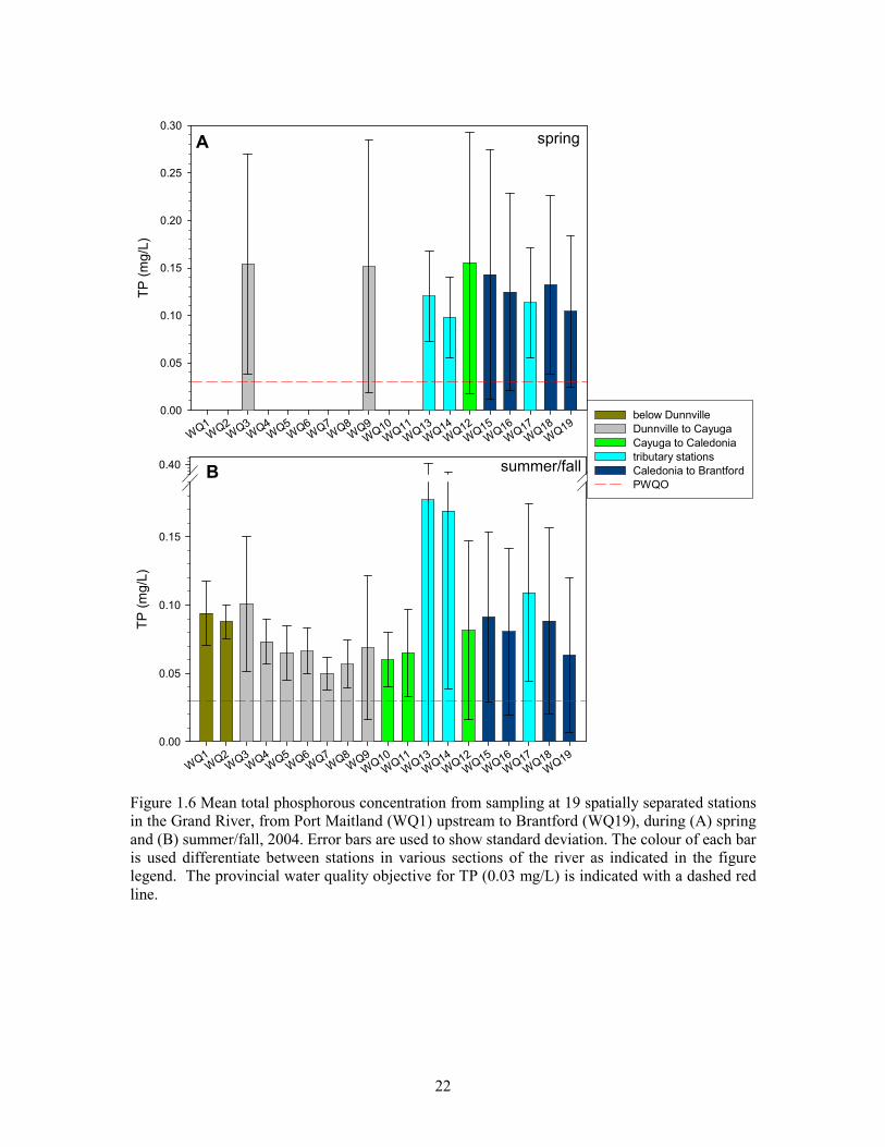
22
spring
WQ1
WQ2
WQ3
WQ4
WQ5
WQ6
WQ7
WQ8
WQ9
WQ10
WQ11
WQ13
WQ14
WQ12
WQ15
WQ16
WQ17
WQ18
WQ19
TP
(m
g/L
)
0.00
0.05
0.10
0.15
0.20
0.25
0.30
summer/fall
WQ1
WQ2
WQ3
WQ4
WQ5
WQ6
WQ7
WQ8
WQ9
WQ10
WQ11
WQ13
WQ14
WQ12
WQ15
WQ16
WQ17
WQ18
WQ19
TP
(m
g/L
)
0.00
0.05
0.10
0.15
0.40
below Dunnville
Dunnville to Cayuga
Cayuga to Caledonia
tributary stations
Caledonia to Brantford
PWQO
A
B
Figure 1.6 Mean total phosphorous concentration from sampling at 19 spatially separated stations
in the Grand River, from Port Maitland (WQ1) upstream to Brantford (WQ19), during (A) spring
and (B) summer/fall, 2004. Error bars are used to show standard deviation. The colour of each bar
is used differentiate between stations in various sections of the river as indicated in the figure
legend. The provincial water quality objective for TP (0.03 mg/L) is indicated with a dashed red
line.

23
summer/fall
WQ1
WQ2
WQ3
WQ4
WQ5
WQ6
WQ7
WQ8
WQ9
WQ10
WQ11
WQ13
WQ14
WQ12
WQ15
WQ16
WQ17
WQ18
WQ19
TN
(m
g/L
)
0
1
2
3
4
5
6
below Dunnville
Dunnville to Cayuga
Cayuga to Caledonia
tributary stations
Caledonia to Brantford
spring
WQ1
WQ2
WQ3
WQ4
WQ5
WQ6
WQ7
WQ8
WQ9
WQ10
WQ11
WQ13
WQ14
WQ12
WQ15
WQ16
WQ17
WQ18
WQ19
TN
(m
g/L
)
0
1
2
3
4
5
6
7
8
B
A
Figure 1.7. Mean total nitrogen concentration from sampling at 19 spatially separated stations in
the Grand River, from Port Maitland (WQ1) upstream to Brantford (WQ19), during (A) spring
and (B) summer/fall, 2004. Error bars are used to show standard deviation.The colour of each bar
is used differentiate between stations in various sections of the river as indicated in the figure
legend.

24
summer/fall
WQ1
WQ2
WQ3
WQ4
WQ5
WQ6
WQ7
WQ8
WQ9
WQ10
WQ11
WQ13
WQ14
WQ12
WQ15
WQ16
WQ17
WQ18
WQ19
NO
3 (
mg
/L)
0
1
2
3
4
5
6
below Dunnville
Dunnville to Cayuga
Cayuga to Caledonia
tributary sites
Caledonia to Brantford
PWQO
spring
WQ1
WQ2
WQ3
WQ4
WQ5
WQ6
WQ7
WQ8
WQ9
WQ10
WQ11
WQ13
WQ14
WQ12
WQ15
WQ16
WQ17
WQ18
WQ19
NO
3 (
mg
/L)
0
1
2
3
4
5
6
spring
WQ1
WQ2
WQ3
WQ4
WQ5
WQ6
WQ7
WQ8
WQ9
WQ10
WQ11
WQ13
WQ14
WQ12
WQ15
WQ16
WQ17
WQ18
WQ19
NO
2 (
mg/L
)
0.00
0.02
0.04
0.06
0.08summer/fall
WQ1
WQ2
WQ3
WQ4
WQ5
WQ6
WQ7
WQ8
WQ9
WQ10
WQ11
WQ13
WQ14
WQ12
WQ15
WQ16
WQ17
WQ18
WQ19
NO
2 (
mg/L
)
0.00
0.02
0.04
0.06
0.08
A B
C D
Figure 1.8. Mean nitrate and nitrite concentrations from sampling at 19 spatially separated stations in the Grand River, from Port Maitland (WQ1)
upstream to Brantford (WQ19), during spring (A&C; respectively) and summer(B&D; respectively), 2004. Error bars are used to show standard
deviation. The colour of each bar is used to differentiate between stations in various sections of the river as indicated in the figure legend. Federal
(CCME) objectives for each parameter are shown with a red dashed line.
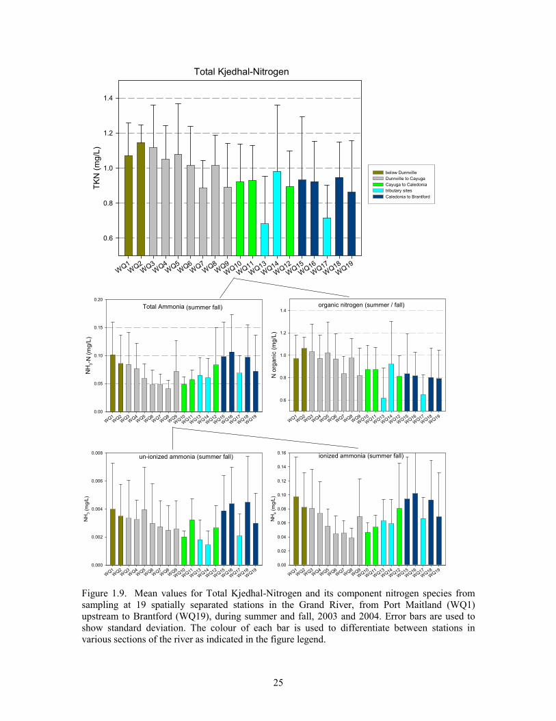
25
organic nitrogen (summer / fall)
WQ1
WQ2
WQ3
WQ4
WQ5
WQ6
WQ7
WQ8
WQ9
WQ10
WQ11
WQ13
WQ14
WQ12
WQ15
WQ16
WQ17
WQ18
WQ19
N o
rgan
ic (
mg
/L)
0.6
0.8
1.0
1.2
1.4
below Dunnville
Dunnville to Cayuga
Cayuga to Caledonia
tributary sites
Caledonia to Brantford
Total Ammonia (summer fall)
WQ1
WQ2
WQ3
WQ4
WQ5
WQ6
WQ7
WQ8
WQ9
WQ10
WQ11
WQ13
WQ14
WQ12
WQ15
WQ16
WQ17
WQ18
WQ19
NH
3-N
(m
g/L
)
0.00
0.05
0.10
0.15
0.20
Total Kjedhal-Nitrogen
WQ1
WQ2
WQ3
WQ4
WQ5
WQ6
WQ7
WQ8
WQ9
WQ10
WQ11
WQ13
WQ14
WQ12
WQ15
WQ16
WQ17
WQ18
WQ19
TK
N (
mg
/L)
0.6
0.8
1.0
1.2
1.4
ionized ammonia (summer fall)
WQ1
WQ2
WQ3
WQ4
WQ5
WQ6
WQ7
WQ8
WQ9
WQ10
WQ11
WQ13
WQ14
WQ12
WQ15
WQ16
WQ17
WQ18
WQ19
NH
4 (
mg/L
)
0.00
0.02
0.04
0.06
0.08
0.10
0.12
0.14
0.16un-ionized ammonia (summer fall)
WQ1
WQ2
WQ3
WQ4
WQ5
WQ6
WQ7
WQ8
WQ9
WQ10
WQ11
WQ13
WQ14
WQ12
WQ15
WQ16
WQ17
WQ18
WQ19
NH
3 (
mg/L
)
0.000
0.002
0.004
0.006
0.008
Figure 1.9. Mean values for Total Kjedhal-Nitrogen and its component nitrogen species from
sampling at 19 spatially separated stations in the Grand River, from Port Maitland (WQ1)
upstream to Brantford (WQ19), during summer and fall, 2003 and 2004. Error bars are used to
show standard deviation. The colour of each bar is used to differentiate between stations in
various sections of the river as indicated in the figure legend.

26
Nitrate
NO3-N (mg/L)
0 1 2 3 4 5 6 7 8 9 10 11 12
Co
un
t
0
10
20
30
40
CCME objective: 2.93 mg/L
Nitrite
NO2-N (mg/L)
0.00 0.02 0.04 0.06 0.08 0.10 0.12 0.14 0.16
Co
un
t
0
10
20
30
40
50
CCME objective: 0.06 mg/L
Un-ionized Ammonia
NH3- (mg/L)
0.000 0.002 0.004 0.006 0.008 0.010 0.012 0.014 0.016 0.018
Co
un
t
0
10
20
30
40
50
60
CCME objective: 0.0165 mg/L)
Figure 1.10. Distribution of nitrate, nitrite, and ammonia (un-ionized) concentrations in from
water collected from the Grand River at Brantford and downstream during 2003 and 2004 (all
stations, all dates; n=389).

27
TP
Aug/04
Aug/11
Aug/18
Aug/25
Sep/01
Sep/08
Sep/15
Sep/22
Sep/29
TP
(m
g/L
)
0.04
0.06
0.08
0.10
0.12
0.14
0.16
0.18
0.20
TSS
Aug/04
Aug/11
Aug/18
Aug/25
Sep/01
Sep/08
Sep/15
Sep/22
Sep/29
TS
S (
mg
/L)
0
20
40
60
80
Nitrate
Aug/04
Aug/11
Aug/18
Aug/25
Sep/01
Sep/08
Sep/15
Sep/22
Sep/29
NO
3 (
mg
/L)
0.8
1.0
1.2
1.4
1.6
1.8
2.0
2.2
2.4
2.6
2.8
WQ3 Surface
WQ3 Bottom
WQ4 Surface
WQ4 Bottom
WQ5 Surface
WQ5Bottom
WQ6 Surface
WQ6 Bottom
WQ7 Surface
WQ7 bottom
WQ8 Surface
WQ8 bottom
A B
C
Figure 1.11. Concentration of total phosphorus (A), nitrate (B), and total suspended solids (C) at
the surface and at depth, from 6 locations within the Grand River during August and September,
2003. Solid lines are used to represent samples taken just below the surface while dashed lines
represent samples collected 0.5-m above the substrate.

28
Total Suspended Solids (mg/L)
0 100 200 300
To
tal P
hosp
horu
s (
mg/L
)
0.0
0.1
0.2
0.3
0.4
0.5
0.6
y = 0.0016x + 0.0403
R2 = 0.7283
Figure 1.12. Relationship between total suspended solids and total phosphorus in water samples
collected in the Grand River downstream of Brantford during 2003 and 2004. (n= 392; p <
0.0001)

29
Station ID
WQ1
WQ2
WQ3
WQ4
WQ5
WQ6
WQ7
WQ8
WQ9
WQ10
WQ11
WQ13
WQ14
WQ12
WQ15
WQ16
WQ17
WQ18
WQ19
N:P
0
20
40
60
80
100
120Below Dunnville
Dunnville to Cayuga
Cayuga to Caledonia
Tributary sites
Caledonia to Brantford
WQ1
WQ2
WQ3
WQ4
WQ5
WQ6
WQ7
WQ8
WQ9
WQ10
WQ11
WQ13
WQ14
WQ12
WQ15
WQ16
WQ17
WQ18
WQ19
Me
an
su
mm
er/
fall
TP
0.04
0.06
0.08
0.10
0.12
0.14
0.16
0.18
0.20
0.22
Mean Total Phosphorus
Mea
n s
um
mer/
fall
TN
1.5
2.0
2.5
3.0
3.5
4.0
4.5
Mean Total Nitrogen
Figure 1.13. The relationship between nitrogen and phosphorus at 19 spatially separated
stations in the Grand River, from Port Maitland (WQ1) upstream to Brantford (WQ19),
during summer and fall, 2003 and 2004. Total nitrogen and total phosphorus are considered
separately as overall mean values at each station (top) and as a ratio (TN:TP). Error bars are
used to show standard deviation. The colour of each bar is used to differentiate between
stations in various sections of the river as indicated in the figure legend.

30
TSS (mg/L)
0 50 100 150 200 250 300
Co
un
t
0
20
40
60
80
100
CCME objective: 25 mg/L
Figure 1.14. Distribution of total suspended solid (TSS) concentrations in from water collected
from the Grand River at Brantford and downstream during 2003 and 2004 (all stations, all dates;
n=402).

31
B - summer/fall
WQ1
WQ2
WQ3
WQ4
WQ5
WQ6
WQ7
WQ8
WQ9
WQ10
WQ11
WQ13
WQ14
WQ12
WQ15
WQ16
WQ17
WQ18
WQ19
TS
S (
mg
/L)
0
50
100
150
200
250
300
below Dunnville
Dunnville to Cayuga
Cayuga to Caledonia
tributary sites
Caledonia to Brantford
A- spring
WQ3
WQ9
WQ13
WQ14
WQ12
WQ15
WQ16
WQ17
WQ18
WQ19
TS
S (
mg/L
)
0
50
100
150
200
250
300
Figure 1.15. Box plots of total suspended solids (TSS) from sampling stations in the Grand River,
from Port Maitland (WQ1) upstream to Brantford (WQ19), during A: Spring (2004) and B: Summer
and fall (2003 and 2004). Mean values are indicated with a red, dotted line. Median values are
indicated with a straight line. The top and bottom edges of each box define the 25th and 75
th percentile
value while the whisker bars describe the 10th and 90
th percentile values. Outliers, where they exist,
are shown with solid dots. The grey background is used to designate values that meet the CCME
guideline of 25 mg/L TSS. The colour of each box is used differentiate between stations in various
sections of the river as indicated in the figure legend.

32
B - summerfall
WQ1
WQ2
WQ3
WQ4
WQ5
WQ6
WQ7
WQ8
WQ9
WQ10
WQ11
WQ13
WQ14
WQ12
WQ15
WQ16
WQ17
WQ18
WQ19
Y D
ata
0
20
40
60
80
100
120
140
below Dunnville
Dunnville to Cayuga
Cayuga to Caledonia
tributary sites
Caledonia to Brantford
A - spring
WQ1
WQ2
WQ3
WQ4
WQ5
WQ6
WQ7
WQ8
WQ9
WQ10
WQ11
WQ13
WQ14
WQ12
WQ15
WQ16
WQ17
WQ18
WQ19
Cl
- (m
g/L
)
0
20
40
60
80
100
120
140
Figure 1.16. Box plots of chloride (Cl-) values from sampling stations in the Grand River, from Port Maitland (WQ1) upstream to Brantford
(WQ19), during A: Spring (2004) and B: Summer and fall (2003 and 2004). Mean values are indicated with a red, dotted line. Median
values are indicated with a straight line. The top and bottom edges of each box define the 25th and 75
th percentile value while the whisker
bars describe the 10th and 90
th percentile values. Outliers, where they exist, are shown with solid dots. The colour of each box is used
differentiate between stations in various sections of the river as indicated in the figure legend.

33
WQ1
WQ2
WQ3
WQ4
WQ5
WQ6
WQ7
WQ8
WQ9
WQ10
WQ11
WQ13
WQ14
WQ12
WQ15
WQ16
WQ17
WQ18
WQ19
pH
(S
U)
6.0
6.5
7.0
7.5
8.0
8.5
9.0
below Dunnville
Dunnville to Cayuga
Cayuga to Caledonia
tributary sites
Caledonia to Brantford
Figure 1.17. Box plots of pH from sampling stations in the Grand River, from Port Maitland (WQ1)
upstream to Brantford (WQ19), during summer and fall (2003 and 2004). Mean values are indicated
with a red, dotted line. Median values are indicated with a straight line. The top and bottom edges of
each box define the 25th and 75
th percentile value while the whisker bars describe the 10
th and 90
th
percentile values. Outliers, where they exist, are shown with solid dots. The grey background is used
to designate values that fall within the CCME guideline range of 6.5 to 8.5 SU. The colour of each
box is used differentiate between stations in various sections of the river as indicated in the figure
legend.

34
WQ1
WQ2
WQ3
WQ4
WQ6
WQ7
WQ9
WQ13
WQ14
WQ12
WQ15
WQ16
WQ17
WQ19
CF
U/1
00
mL
0
100
200
300
400
500
600
below Dunnville
Dunnville to Cayuga
tributary sites
Cayuga to Caledonia
Caledonia to Brantford
MOE - beach closing
Figure 1.18. E.coli, as indexed by total coliform counts, in samples collected from sampling at 14
spatially separated stations in the Grand River, from Port Maitland (WQ1) upstream to Brantford
(WQ19), on August 31, 2004. The colour of each bar is used to differentiate between stations in
various sections of the river as indicated in the figure legend.

35
1. 7 Tables

36
Table 1.1. Sampling dates on which water was collected for water chemistry analysis from 19 stations located in the Grand River, at
Brantford and downstream to Port Maitland, 2003 and 2004. Shaded dates indicate occasions on which water was collected from both
the surface and at 0.5-m above the substrate. “A” and “B” are used to designate separate locations in close proximity (<75m).
WQ1 WQ2 WQ4 WQ5 WQ6 WQ7 WQ8 WQ10 WQ11 WQ12 WQ13 WQ14 WQ15 WQ16 WQ17 WQ18 WQ19
DATE A B A B
(dd-mmm-yy) * * * * * *
22-Jul-03
05-Aug-03
06-Aug-03
13-Aug-03
20-Aug-03
25-Aug-03
02-Sep-03
09-Sep-03
15-Sep-03
23-Sep-03
29-Sep-03
07-Oct-03
15-Oct-03
16-Oct-03
21-Oct-03
27-Oct-03
19-Nov-03
04-Mar-04
08-Mar-04
09-Mar-04
11-Mar-04
18-Mar-04
25-Mar-04
30-Mar-04
01-Apr-04
06-Apr-04
14-Apr-04
20-Apr-04
27-Apr-04
02-Jun-04
17-Jun-04
15-Jul-04
27-Jul-04
10-Aug-04
19-Aug-04
31-Aug-04
15-Sep-04
29-Sep-04
13-Oct-04
25-Oct-04
WQ3 WQ9
Station ID Number
Below
Dunnville DamAbove Dunnville dam to Cayuga Cayuga to Caledonia Caledonia to Brantford

37
Table 1.2. Descriptive statistics for water quality parameters measured at 19 stations in the Grand River below Brantford, during 2003
(summer and fall) and 2004 (spring, summer and fall). Values are given in units of mg/L.
Mean Median Mode
Standard
Error
Standard
Deviation
Sample
Variance Range Minimum Maximum n
Confidence
Level (95.0%)
Total Phosphorus (TP)
Spring 0.13 0.10 0.05 0.009 0.099 0.010 0.48 0.03 0.51 115 0.018
Summer 0.10 0.08 0.07 0.006 0.070 0.005 0.36 0.02 0.38 134 0.012
Fall 0.09 0.06 0.06 0.009 0.105 0.011 1.03 0.01 1.04 153 0.017
SummerFall 0.09 0.07 0.06 0.005 0.091 0.008 1.03 0.01 1.04 287 0.011
OVERALL 0.10 0.08 0.06 0.005 0.095 0.009 1.03 0.01 1.04 402 0.009
Total Nitrogen (TN)
Spring 4.97 5.26 5.12 0.154 1.655 2.739 10.40 1.42 11.82 115 0.306
Summer 3.14 3.10 NA 0.115 1.254 1.571 5.80 0.82 6.61 119 0.228
Fall 3.35 3.34 3.49 0.110 1.357 1.842 6.93 0.47 7.40 153 0.217
SummerFall 3.26 3.26 2.14 0.080 1.314 1.728 6.93 0.47 7.40 272 0.157
OVERALL 3.77 3.51 2.14 0.082 1.623 2.633 11.35 0.47 11.82 387 0.162
TKN
Spring 0.93 0.88 1.10 0.031 0.329 0.108 1.64 0.38 2.02 115 0.061
Summer 0.91 0.88 0.88 0.023 0.262 0.069 1.71 0.44 2.14 134 0.045
Fall 0.94 0.91 0.74 0.021 0.262 0.069 1.44 0.33 1.77 153 0.042
SummerFall 0.93 0.89 0.74 0.015 0.262 0.069 1.81 0.33 2.14 287 0.030
OVERALL 0.93 0.88 0.74 0.014 0.282 0.080 1.81 0.33 2.14 402 0.028
Ammonia (NH3-N)
Spring 0.18 0.16 0.02 0.014 0.154 0.024 0.67 0.01 0.68 115 0.028
Summer 0.07 0.06 0.05 0.004 0.048 0.002 0.21 0.02 0.23 149 0.008
Fall 0.08 0.06 0.06 0.004 0.054 0.003 0.27 0.02 0.28 153 0.009
SummerFall 0.07 0.06 0.05 0.003 0.051 0.003 0.27 0.02 0.28 302 0.006
OVERALL 0.07 0.06 0.05 0.002 0.050 0.002 0.27 0.02 0.28 451 0.005
Nitrite (NO 2 )
Spring 0.04 0.04 0.03 0.002 0.018 0.000 0.08 0.01 0.09 115 0.003
Summer 0.03 0.02 0.01 0.002 0.025 0.001 0.14 0.01 0.14 121 0.004
Fall 0.02 0.02 0.02 0.001 0.015 0.000 0.08 0.00 0.08 153 0.002
SummerFall 0.03 0.02 0.02 0.001 0.020 0.000 0.14 0.00 0.14 274 0.002
OVERALL 0.03 0.03 0.01 0.001 0.020 0.000 0.14 0.00 0.14 389 0.002
Nitrate (NO 3 )
Spring 4.00 4.28 4.42 0.137 1.471 2.165 10.08 0.42 10.50 115 0.272
Summer 2.20 2.09 1.42 0.111 1.218 1.484 5.57 0.00 5.57 121 0.219
Fall 2.39 2.44 2.16 0.100 1.240 1.538 5.84 0.02 5.86 153 0.198
SummerFall 2.30 2.32 1.42 0.074 1.232 1.517 5.86 0.00 5.86 274 0.146
OVERALL 2.80 2.59 1.42 0.077 1.517 2.302 10.50 0.00 10.50 389 0.151
Chloride (Cl-)
Spring 54.76 53.00 25.00 2.362 25.332 641.695 100.00 20.00 120.00 115 4.679
Summer 75.73 75.05 107.00 2.359 25.192 634.618 97.20 22.80 120.00 114 4.674
Fall 83.90 86.80 104.00 1.966 24.323 591.594 105.10 24.90 130.00 153 3.885
SummerFall 80.41 83.80 104.00 1.529 24.981 624.026 107.20 22.80 130.00 267 3.010
OVERALL 72.69 74.90 104.00 1.417 27.686 766.520 110.00 20.00 130.00 382 2.785
Total Suspended Solids (TSS)
Spring 52.22 35 18 4.882 52.356 2741.172 265 2 267 115 9.672
Summer 36.43 26 20 3.495 40.458 1636.879 231 2 233 134 6.913
Fall 27.92 21 15 2.288 28.298 800.770 253 2 255 153 4.520
SummerFall 31.90 24 15 2.049 34.711 1204.884 253 2 255 287 4.033
OVERALL 37.71 26 20 2.070 41.511 1723.184 265 2 267 402 4.070
pH
Spring 7.98 7.98 7.90 0.021 0.224 0.050 1.27 7.23 8.50 115 0.041
Summer 8.01 8.01 8.10 0.031 0.315 0.099 1.50 7.20 8.70 101 0.062
Fall 8.03 8.10 8.10 0.023 0.283 0.080 2.15 6.45 8.60 153 0.045
SummerFall 8.02 8.10 8.10 0.019 0.296 0.087 2.25 6.45 8.70 254 0.037
OVERALL 8.01 8.03 8.10 0.014 0.276 0.076 2.25 6.45 8.70 369 0.028

38
Table 1.3. A comparison of descriptive statistics for select water quality parameters measured in the Grand River between Brantford and Port
Maitland during i) an intensive survey at 19 stations in 2003 and 2004 and ii) regular PWQMN sampling at 3 stations between 2000 and 2005.
Mean Median Mode
Standard
Error
Standard
Deviation
Sample
Variance Range Minimum Maximum n
Total Phosphorus (TP)
Intensive (03-04) 0.10 0.08 0.06 0.005 0.095 0.009 1.03 0.01 1.04 402
PWQMN (00-05) 0.11 0.09 0.06 0.005 0.077 0.006 0.65 0.01 0.66 210
TKN
Intensive (03-04) 0.93 0.88 0.74 0.014 0.282 0.080 1.81 0.33 2.14 402
PWQMN (00-05) 1.03 0.96 0.92 0.027 0.390 0.152 2.65 0.36 3.01 210
Nitrite (NO2)
Intensive (03-04) 0.03 0.03 0.01 0.001 0.020 0.000 0.14 0.00 0.14 389
PWQMN (00-05) 0.05 0.04 0.03 0.002 0.032 0.001 0.19 0.00 0.19 204
Nitrate (NO3)
Intensive (03-04) 2.80 2.59 1.42 0.077 1.517 2.302 10.50 0.00 10.50 389
PWQMN (00-05) 3.24 3.08 3.18 0.107 1.545 2.389 6.88 0.26 7.14 207
Chloride (Cl-)
Intensive (03-04) 72.69 74.90 104.00 1.417 27.686 766.520 110.00 20.00 130.00 382
PWQMN (00-05) 81.37 79.80 90.40 2.541 35.025 1226.732 278.90 6.10 285.00 190
pH
Intensive (03-04) 8.01 8.03 8.10 0.014 0.276 0.076 2.25 6.45 8.70 369
PWQMN (00-05) 8.29 8.29 8.34 0.009 0.124 0.015 0.66 7.93 8.59 207

39
2.0 Primary production – planktonic algae (chlorophyll-a)
2.1 Introduction
Phytoplankton play an important role in aquatic food webs; linking nutrients and energy
(sunlight) with filter feeders, zooplankton, forage fish and, secondarily, the microbial loop. In
extremely productive waters, excessive growth of algae can have detrimental effects. These
effects can either be direct, through shading and reduced water clarity (Lorenzen 1972), or
indirect when settled, ungrazed, dead phytoplankton provide substrate on which oxygen
consuming microbes can thrive thereby reducing or depleting dissolved oxygen (USEPA, 2003).
Additionally, photosynthesis and respiration by living algae can drastically alter the oxygen
regime of surface waters.
While many studies of algal growth in riverine systems have focussed on substrate-attached
periphyton (Chételat 1999, Dodds 2006), algal production in the turbid waters of the lower Grand
is necessarily dominated by planktonic algae. Planktonic algal biomass, as represented by
chlorophyll-a (Chl-a) concentration in the water column, has traditionally been included in the
suite of measures used to describe the trophic state of a water body.
Chlorophyll-a concentrations in the Southern Grand River (SGR) were measured in 2003 and
2004 to describe trophic status by serving as an analog for planktonic algal production and thus to
better characterize the ecosystem and aquatic habitat downstream of Brantford. Knowing the
abundance of phytoplankton would help to help to link observations made during water
chemistry, benthic invertebrate, and oxygen profiling. Sampling was designed to look for change
along the spatial gradient of the river, as well as changes through time and/or with depth.
2.2 Methods
Water sampling
A subset of the water quality sampling stations (described above in 1.1; Water Quality) were
chosen for concurrent chlorophyll-a measures. These stations were given labels prefixed with a
“C” and which correspond to WQ-station labels (from section 1.0) as follows:
C1 – WQ1 (Port Maitland)
C2 – WQ2 (Betamik Harbour)
C3 – WQ3 (Dunnville; above dam)
C4 – WQ6 (Dunnville to Cayuga; mid-way)
C5 – WQ9 (Cayuga)
C6 – WQ12 (York)
C7 – WQ18 (Brantford; Newport bridge)
In 2003, chlorophyll-a (Chl-a) in surface waters was measured at seven stations between Port
Maitland and Brantford on an approximate bi-weekly basis between July 22 and October 27 (6
occasions; Table 2.1). On some alternate weeks, at three of these stations, (C1, C4 and C7),
water was collected at both the surface and at depth (0.5m off of the bottom) in order to describe
any differences within the water column. In 2004, water for chlorophyll analysis was only
collected at stations between Cayuga and Port Maitland (Stns C1-C5) on 13 occasions (bi-

40
weekly) between June 15 and October 20 (Table 2.1). For logistic reasons not all stations were
sampled on all dates.
As described in the methodology for water chemistry sampling (Section 1.2), equal volumes of
sub-surface (0.5m depth) water, collected at four locations across the width of the river, were
combined and mixed prior to the filling of sample bottles. Samples at depth were collected using
a Van-Dorn bottle lowered to a depth 0.5-m above the bottom.
Sample analysis
All water samples were placed on ice in the dark, transported to the lab, and processed within 12
hours. Processing involved mixing of the water sample followed by filtration of 500 mL through
a glass fibre filter (Whatman GF/C; median retention size of approx 0.2 um) using a Millipore
filter apparatus. Duplicate filter papers were placed into plastic whirl-pac bags with silica-gel
absorbent and frozen until analysis (< 4 months) at the OMNR lab in Wheatley.
Samples filters were homogenized in 90% acetone and the resulting extracts were analysed
spectrophotometrically as per Strickland and Parsons (1972). The average of the replicate
samples was used for comparison.
Results and discussion will centre on chlorophyll-a concentrations which have been corrected to
exclude contributions from phaeopigments (which represent the breakdown products of a number
of chlorophylls). Uncorrected values, sometimes described as “total chlorophyll” are provided in
Appendix B-1 for reference. While recognizing the lack of consensus of the most accurate / least
misleading way of quantifying algal biomass/Chl-a, it was felt that the methods used in this study
are sufficient for discussing trophic classification, and short term and spatial gradients within the
system. The often larger “un-corrected” values in the appendix give an idea of both living and
dead phytoplankton and are valuable when considering the ability of all algal cells (living or
dead) to contribute to light attenuation in the water column. Attention to specific details of this
analytical methodology will be important for future monitoring which involves tracking long term
change.
Classifying trophic state based on chlorophyll-a concentration.
Describing water bodies based on their nutrient regimes and productivity has a long history in
limnology. The classic lake classifications of oligotrophic, mesotrophic and eutrophic have also
been applied to lotic systems. The classification of “eutrophic”, carries with it the negative
connotation of being “too productive” and usually implies negative aspects of plant (algal)
growth (blooms) and disrupted oxygen regimes, particularly due to the metabolism of
heterotrophs (microbial loop) consuming abundant dead algal cells and resulting in hypoxia or
anoxia.
Placing bounds on each state, using chlorophyll-a, has been done by a number of authors
(Appendix A-3). For the purpose of this report, that proposed by Wetzel will be used as follows:
Oligotrophic - 0.3–3 µg/L
Mesotrophic - 2–15 µg/L
Eutrophic - >10 µg/L
Additionally, the concept of Hyper-eutrophic (>15 µg/L) (Ryding and Rast. 1989, Leach et al.
1977) - will be referred to.
Statistical comparisons
For each year, mean station Chl-a was compared between stations using a one-way ANOVA after
first log-normalizing the data (Anderson-Darling) and confirming homogeneity of variance
(Bartlett's test). Post hoc confirmations of significant differences were identified using Fisher’s
LSD tests.

41
2.3 Results
Concentrations of chlorophyll-a, measured during this survey (both years, n= 117), ranged
between 0.74 and 64.49 µg/L. The overall mean, median and mode were 20.05, 18.78, and 16.78
µg/L; respectively.
Spatial gradient in Chl-a concentration
An obvious trend of increasing mean Chl-a concentration was apparent as one progressed
downstream from Brantford (2003) or Cayuga (2004) to Port Maitland (Figure 2.1). Upstream
stations C7 (Brantford at Newport Bridge) and C6 (York), sampled in 2003 only, had mean
concentrations (2.67 - 7.3 µg/L) indicative of oligotrophic to mesotrophic waters while those at
downstream stations C5 (Dunnville above dam) to C7 (Port Maitland; 20.4 - 36.0 µg/L) could be
classified as eutrophic to hyper-eutrophic (based on Wetzel 2001). Concentrations at Cayuga (C4)
fell between these and were indicative of mesotrophic waters. The highest annual mean
concentration (36.0 µg/L; n= 13) occurred in 2004 at station C2, located between the Dunnville
dam and Port Maitland. The lowest annual mean concentration (2.67 µg/L; n= 6) occurred in
2003 at station C1, located below the Newport bridge in Brantford.
In 2003, mean Chl-a concentrations at stations downstream of Cayuga (C1, C3 and C4; C2 not
included) were significantly larger than those at Cayuga (C5) and Brantford (C7). Additionally,
the mean at C3 was significantly higher than that at C6; those from C1 and C4 were not (Table
2.2). Similarly, in 2004 mean concentration at the most upstream station measured (Cayuga; C5)
was significantly smaller than those at more downstream stations. The next downstream station
(C4) was significantly smaller than the highest mean station (C2).
Changes in Chl-a with depth
The brief examination of differences in Chl-a concentration between surface water and that at
depth, from four dates in 2003 at stations C3, C4 and C5, showed that planktonic algae were not
restricted to surface waters (Figure 2.2). Concentrations at depth, at C3 and C4 were, on average,
10µg/L less than at the surface. Well mixed waters are suggested on August 25 at station C4,
where Chl-a at the surface (30.2µg/L) was similar to that at 4m depth (27.6µg/L). At C5, the
shallowest station, concentrations on August 13, were actually higher at depth than at the surface.
There were no differences between surface and depth concentrations on September 23, at any
station. Despite being generally lower, most concentrations at depth were still indicative of
eutrophic waters (>10µg/L).
Seasonal changes
In 2003, concentrations at Brantford remained consistently between 2 and 6 µg/L while values at
more downstream stations were considerably greater and varied considerably. Chl-a at Cayuga
peaked in late August and early September before declining (Figure 2.3). Measures at York
(sampled less frequently) were similar to those at Cayuga. Chl-a concentrations mid way between
Cayuga and Dunnville and just above the Dunnville dam also peaked (>25µg/L) between Aug 25
and Sep 9 before dropping off to levels comparable to those at Brantford. The two most
downstream stations (above Dunnville dam and Port Maitland) peaked a second time in mid
October.
In 2004, Chl-a concentration at the most upstream station (C5; Cayuga) again, varied the least,
relative to those further downstream (Figure 2.3). Most stations displayed three peaks throughout
the season in early-mid July, mid August and late September. The highest measures, in excess of

42
50 µg/L were observed immediately above (Aug 9) and below (July 6 and Sept. 23) the Dunnville
dam.
In both years a clear distinction existed between stations C1-C4 and C5-C7 with regard to
maximum values attained and variation; the former being consistently higher and more variable
than the latter.
Comparisons with Lake Erie
By way of contrast with the waters that the Grand empty into, Chl-a concentration on individual
sampling days at station C2 was compared graphically with values obtained concurrently at a
nearshore location in the eastern basin of Lake Erie (Figure 2.4). In addition to the large
differences in concentration, it is apparent that there is considerable more variation in the river
water measures.
2.4 Discussion
The SGR has very high primary productivity; large concentrations of planktonic algae are
produced in the waters downstream of Brantford. Relative Chl-a concentration changes not only
along the spatial gradient of the river but seasonally at individual locations.
The spatial pattern (increasing Chl-a in a downstream direction) does not mirror the spatial
patterns seen in total phosphorus (TP). In systems where phosphorus limits production (bottom-
up control), TP is usually predictive of chlorophyll (Dillon and Rigler 1974). TP was often just
as high at Brantford as it was at Dunnville; other factors are influencing the disparity in the
Chl:TP ratio. One obvious difference is the change in flow that occurs downstream of Cayuga.
Whereas the river moves faster through Brantford and York, it slows and widens beyond its
historic channel where it enters the backwater of the Dunnville dam, the influence of which is
measurable upstream to the highway #3 bridge in Cayuga (Kennaley et al. 1979). The reservoir
effect results in an increase in retention time to almost 3 days from a calculated historical time of
less than 8 hours (Gilbert et al. 2004). Unfortunately absent from the survey were stations in the
reservoir formed immediately upstream of the Caledonia dam which would have served as a good
comparison to station C3. Deviations in the expected Chl: TP ratio may reflect the alternating
predominance of periphyton production vs planktonic algae production as one moves
downstream, alternating between lotic and lentic conditions (Vannote et al. 1980).
Although classified as eutrophic based on phosphorus concentrations, the two most upstream
stations (at York and Brantford) can be classified as mesotrophic to oligotrophic based on Chl-a
data. Dodds (2006) however cautions about underestimating trophic state by focussing on
planktonic production in lotic waters.
Concentrations of chlorophyll-a in the more lentic waters of the Dunnville reservoir and lake-
effect zone downstream of Dunnville indicate that these areas are hyper-eutrophic.
Phytoplankton turbidity contributes to light attenuation from other suspended particles, further
limiting the growth of periphyton and submerged macrophytes (Knapton, R.W. 1993, Gilbert and
Ryan 2007). The occurrence of diurnal dissolved oxygen fluctuations in surface waters (see
section 5.0; Temperature and Oxygen), in the near absence of periphyton and submerged
macrophytes, is further evidence of high planktonic algal biomass and reinforces the designation
of “hyper-eutrophic”. Similarly, there is evidence for periods of low dissolved oxygen
concentration at depth, consistent with the oxygen demand that would accompany the settling and
decomposition of large quantities of unconsumed algal cells (see following sections).

43
The high planktonic algal biomass of the river estuary stands in stark contrast to the generally
nutrient poor and (relatively) low phytoplankton biomass waters of the eastern basin of Lake Erie
into which the river flows. Although the nutrient pattern of the river can be detected in nearshore
waters for kilometres along the shoreline (T. Howell OMOE; pers comm.) increased water clarity
and changes in nutrient cycling in the lake result in a shift in primary production toward attached
filamentous algae (Higgins et al. 2005).
Many of the negative effects of high nutrients in the SGR may be attributable to the change in
hydrology imposed by the dam at Dunnville. The increased retention time of the lower energy
reservoir provides an incubation environment where planktonic algae can flourish resulting in
related unfavourable environmental conditions (see following sections). Similar conditions are
predicted upstream of the dam at Caledonia. If the Dunnville dam were not creating this
reservoir, there would still be a degree of slowing and widening of the river where the river and
lake mix however the dynamic aspect of the lake seiche would create a more physically energetic
environment unlike that which presently exists above Dunnville.
2.5 References
Dillon, P.J., and F. H. Rigler. 1974. Phosphorus–chlorophyll relationship in lakes. Limnol.
Oceanogr. 19(5): 767–773.
Dodds, W.K. 2006. Eutrophication and trophic state in rivers and streams. Limnol. Oceanogr.,
51(1, part 2), 2006, 671–680
Gilbert J.M., Dunn, G.C. and P. A. Ryan. 2004. Surface morphology of the wetlands along the
Lower Grand River between Cayuga and Dunnville. Report for the Ontario Ministry of
Natural Resources, Lake Erie Management Unit, Port Dover, ON
Gilbert, J.M., and P.A., Ryan. 2007. Southern Grand River Wetland Report: ecological
assessment of the wetlands within the southern Grand River between Cayuga and
Dunnville. Ministry of Natural Resources internal report. Port Dover, ON. 37pp +
appendixes
Higgins, S.N., Howell, T.E., Hecky, R.E., Guildford, S.J. and R.E. Smith, 2005. The wall of
green: the status of Cladophora on the northern shores of Lake Erie’s eastern basin, 1995-
2002. J. Great Lakes Res. 31: 547-563.
Kennaley, L., Lewies, R., McLarty, A., and P. Mason. 1979. Environmental appraisal of the
removal of Dunnville dam based on available literature of the area between Dunnville
dam and the town of Cayuga. Report of the Regional Municipality of Haldimand-
Norfolk, Ontario Ministry of Natural Resources, Ontario Ministry of the Environment
and the Grand River Conservation Authority.
Knapton, R.W. 1993. Mapping of submerged vegetation and benthic invertebrates in the
Dunnville Marshes. Long Point Waterfowl and Wetlands Research Fund Report.
Prepared for Canadian Wildlife Service, London ON. 21p + appendixes.

44
Leach, J.H., Johnson, M.G., Kelso, J.R.M. Hartman, J., Mumann, W., and B. Entz. 1977.
Responses of percid fishes and their habitats to eutrophication. J. Fish. Res. Board Can.
1964-1971
Lorenzen, C. J. 1972. Extinction of light in the ocean by phytoplankton. Journal of Conservation
34:262-267.
Ryding, S. O. and W. Rast. 1989. The control of eutrophication of lakes and reservoirs. Man and
the Biosphere Series, Volume 1, UNESCO, Parthenon Publication Group, Park Ridge,
New Jersey. 314 pp.
Stickland, J.D.H. and T.R. Parsons. 1972. A practical handbook of seawater analysis. 2nd ed.
Bull. Fish. Res. Board Can. 167:310
Vannote, R.L., Minshall, G.W., Cummins, K.W., Dedell, J.R. and C.E. Cushing. 1980. The River
Continuum Concept. Can.J.Fish.Aquat.Sci. 37:130-137.
Wetzel, R. G. 2001. Limnology–Lake and River Ecosystems, 3rd Edition. Academic Press, New
York, New York.

45
2.6 Figures

46
Station
C7 C6 C5 C4 C3 C2 C1
Ch
loro
ph
yll-
a (
µg/L
)
0
10
20
30
40
50 2003
2004
Eutrophic boundary (Wetzel 2001)
Oligotrophic boundary
n= 6 5 12 13 12 1 512 12 13 13 13
ns ns
downstream of DunnvilleCayuga to DunnvilleYorkBrantford
Figure 2.1 Mean chlorophyll-a (Chl-a) concentration at seven stations within the lower reaches of
the Grand River, 2003-2004. Stations C6 and C7 were not sampled in 2004. Chl-a values have
been corrected to remove the influence of phaeopigments. Error bars represent the standard
deviation. Stations are presented (left to right) from the most upstream (C7; Brantford) to the
most downstream (C1; Port Maitland at Lake Erie).

47
Aug 1 Sep 1 Oct 1
Ch
loro
ph
yll-
a (
µg/L
)
0
10
20
30
40
50
C3 -Surface
C3 -Depth (1.5m)
C4 -Surface
C4 -Depth (4m)
C5 -Surface
C5 -Depth (1m)
Eutrophic boundary (Wetzel 2001)
Oligotrophic boundary
Figure 2.2. Chlorophyll-a (Chl-a) concentration at three stations (C3-C5) within the lower reaches
of the Grand River, 2003. Chl-a values have been corrected to remove the influence of
phaeopigments and represent the mean of two separate water filtrations and spectrophotometric
readings.

48
2003
Jun 1 Jul 1 Aug 1 Sep 1 Oct 1 Nov 1
Chlo
rop
hyll-
a (
µg/L
)
0
10
20
30
40
50
60
70
C1 (Port Maitland)
C2 (Betamik harbour)
C3 (Dunnville above dam)
C4 (mid-way Dunville to Cayuga)
C5 (Cayuga)
C6 (York)
C7 (Brantford at Newport Bridge)
Eutrophic boundary (Wetzel 2001)
Oligotrophic boundary
2004
Jun 1 Jul 1 Aug 1 Sep 1 Oct 1 Nov 1
Ch
loro
ph
yll-
a (
µg
/L)
0
10
20
30
40
50
60
70
Figure 2.3 Seasonal patterns of chlorophyll-a (Chl-a) concentration at seven stations (C1-C7) within the
lower reaches of the Grand River, 2003-2004. Chl-a values have been corrected to remove the influence of
phaeopigments and represent the mean of two separate water filtrations and spectrophotometric readings.

49
2004
May 1 Jun 1 Jul 1 Aug 1 Sep 1 Oct 1 Nov 1
Ch
loro
ph
yl (µ
g/L
)
0
10
20
30
40
50
60
70
L.E. eastern basin nearshore
GR station C2
Figure 2.4. Chlorophyll-a (Chl-a) concentration at Grand River sample station C2 relative to
concentrations from epilimnetic waters at a nearshore location (Lake Erie Committee, Forage
Task Group; LTLA station 15; 7m depth) in the eastern basin of Lake Erie, May- October, 2004.
Chl-a values have been corrected to remove the influence of phaeopigments and represent the
mean of two spectrophotometric readings.

50
2.7 Tables

51
Table 2.1. Dates on which water sampling for chlorophyll-a (Chl-a) occurred at seven stations (C1-C7) within the lower reaches of the Grand
River during 2003 and 2004. The portion of the water column sampled is indicated (either surface or at depth). Four sub-surface collections across
the width of the river were mixed to create a composite sample for filtering.
Date (dd-MMM-YY) Surface Depth Surface Depth Surface Depth Surface Depth Surface Depth Surface Depth Surface Depth
2003
23-Jul-03 X X X
6-Aug-03 X X X X X X
13-Aug-03 X X X X X X
25-Aug-03 X X X X X X
2-Sep-03 X X X X X X
9-Sep-03 X X X X X X
15-Sep-03 X X X X X X
23-Sep-03 X X X X X
29-Sep-03 X X X
7-Oct-03 X X X
16-Oct-03 X X X X X X
21-Oct-03 X X X
27-Oct-03 X X X X X X
2004
15-Jun-04 X X X
23-Jun-04 X X X X X
29-Jun-04 X X X X X
06-Jul-04 X X X X X
13-Jul-04 X X X X X
20-Jul-04 X X X X X
26-Jul-04 X X X X X
03-Aug-04 X X X X X
09-Aug-04 X X X X X
23-Aug-04 X X X X X
30-Aug-04 X X X X X
23-Sep-04 X X X X X
20-Oct-04 X X X X X
Cayuga York
C6
Brantford
C7
Betamik Dun-above dam
C4
mid way (RV)
C1 C2 C5C3
Port Maitland

52
Table 2.2. One-way ANOVA comparison of annual mean chlorophyll-a concentrations at Grand River sampling stations (C1-C7). Data was log-
normalized (Anderson-Darling) prior to comparison and tested for homogeneity of variance (Bartlett’s). Individual differences were identified
using Fishers LSD test. Note Station C2 not included in 2003 due to insufficient replicate measures. (“sd” indicates statistically different at
p<0.05, “*” indicates no statistical difference.
2003
C1
C3
C4
C5
C6
C7
C1
na
*
*
sd
*
sd
C3
-
na
*
sd
sd
sd
C4
-
-
na
sd
*
sd
C5
-
-
-
na
*
*
C6
-
-
-
-
na
*
2004
C1
C2
C3
C4
C5
C1
na
*
*
*
sd
C2
-
na
*
sd
sd
C3
-
na
*
sd
C4
-
-
-
na
sd

53
3.0 Benthic Invertebrates
3.1 Introduction
Benthic invertebrate community structure is a commonly used indicator of aquatic habitat health,
particularly as it changes relative to the level of nutrients in the surrounding water. Previous
surveys of benthic invertebrates in the Southern Grand River (SGR) have been limited to specific
areas below Dunnville dam; in the Dunnville Marshes (Knapton 1993) at the river mouth (MOE,
2002). Wetlands adjacent to the main channel above and below the dam were surveyed in 2004
(Gilbert and Ryan 2007). To further efforts to characterize habitat quality in the SGR, surveys of
the benthic invertebrate community in the main channel were conducted in 2002 and 2003.
In designing the sampling strategy, attempts were made to recognize the large number of
variables able to impact/shape the benthic community as well as acknowledge the patchiness in
distribution characteristic of many benthic species. As substrate type is a strong determinant of
community structure, it was decided that sampling sites would be confined to the section of river
from Cayuga downstream to Port Maitland where the substrate is comprised mainly of
unconsolidated sand/silt and fine grained organic muck. Upstream of Cayuga, there exist large
stretches of exposed bedrock, cobble and rubble. Cayuga represents the theoretical upstream
limit of the, pre-Dunnville dam, lake effect zone (based on mid-channel elevation and chart
datum lake levels; Gilbert et al. 2004).
The objectives of the survey included the following:
i) To compare benthic communities along a spatial gradient of the main river channel (and
relative to the dam at Dunnville) with regard to indicator species, common invertebrate indices
(e.g. Hilsenhoff index of organic pollution), species diversity and relative abundance,
ii) To make comparisons to previous studies.
iii) To describe densities and available species with regard to diet needs of benthivorous fish
species (and life stages).
iv) To describe trophic status based on the presence/absence of indicator species.
With regard to ranking the SGR ecosystem relative to other tributary/Great Lake interface areas;
lack of data from an appropriate undisturbed reference sites precluded methods of analysis such
as those suggested in the Ontario Benthic Biomonitoring Network protocol (Jones et al. 2004).
3.2 Methods
Five sample sites were chosen to provide a spatial gradient between Cayuga and Port Maitland
and to correspond with locations of concurrent sampling for water quality, algal biomass, and
temperature/oxygen regimes. Two of the stations were located downstream of the Dunnville dam
and the Dunnville water treatment control plant. Three stations were located upstream of
Dunnville; one immediately upstream of the dam, one at Cayuga, and one approximately mid-
way between (Figure 3.1). These sites, labelled B1-B5; correspond with chlorophyll-a stations
C1-C5; respectively (see section 2.0). At each site, four replicate samples were collected at
regularly spaced locations across the width of the channel. Figure 3.2 shows relative channel
width and shape at each site as well as replicate locations from 2003 sampling (2002 replicate

54
locations were not geo-referenced but followed a similar pattern; a transect perpendicular to the
channel).
When attempting to describe the maximum species richness of a benthic community, avoidance
of mid-summer sampling is recommended (Rosenberg et al. 1998). Ideally this would involve
sampling in either early spring (just after ice-out) or late fall. Attempts to conform to this standard
met with limited success due to logistical constraints in each year. In 2002, planned spring
sampling was delayed until July 11th. In 2003, sampling was conducted at the end of the field
season, on October 1st (above dam sites) and 2
nd (below dam sites).
Samples of substrate were obtained using an 8-litre ponar dredge (capture area = 0.215m x
0.245m; Wildco. Ltd) lowered from the bow of a 14-ft Jon-boat. Partial samples, where the ponar
misfired or was not full when retrieved, were discarded in favour of 4 complete samples.
Substrate samples were sieved through a coarse mesh to remove obvious debris such as twigs or
pebbles. The filtrate was then sieved through a 500µm screen before being placed in plastic
bottles and preserved in 10% formalin. Samples were subsequently rinsed, preserved in alcohol,
and picked under microscopes in a lab setting. All collected organisms were delivered to a
recognized consulting service to ensure accurate identification (Bland and Associates, Ltd.,
London, Ontario).
The following parameters were calculated to describe the benthic community:
Density – expressed as #/m2 extrapolated from the area captured by the ponar (0.245m x 0.215m
= 0.053m2);
in order to facilitate comparisons to previous studies. Mean density per site is
reported.
Species Richness (S) – counts of overall number of unique taxa at each site. To give a more
representative picture of an area, replicates were pooled for this count because of the variability
between samples and the patchy distribution of several species. These taxa counts were based,
for the most part on identification to genus or species; higher order identifications were only
counted when no lower classifications occurred within that grouping. Subtotal contributions from
individual taxon groupings were also considered.
Shannon-Weiner Diversity Index and associated measures
H'= -∑(pi)(logepi)
where “pi” is the proportion of individuals in the “ith” taxon of the community
Hmax = ln (S) – represents the maximum H' value given a fixed number of species
(assumes equal contribution from each species.)
Species Evenness (E) = H/Hmax – a measure of equitability, commonly used as a
community descriptor
Hilsenhoff Biotic Index
Hilsenhoff values were calculated in two ways:

55
1. HH- the traditional Hilsenhoff whereby all organisms are used with the limitation that
each replicate must contain at least 100 individuals. Due to the low densities in the study
area, this necessitated the pooling of replicates and the calculation of only one value per
site. This methodology emphasises disparities in relative abundance of individual species
(diversity).
∑=n
txHBI ii
where
xi = number of individuals within a species
ti = tolerance value of a species
n = total number of organisms in the sample
2. HH10max- a modified Hilsenhoff described in Mandaville (2002) whereby the effects of
extremely abundant species are dampened. This method involves capping individual
species counts at 10 and, despite the low densities of the study area, allowed for index
values to be calculated for each replicate and thus statistical comparison to be made
between sites. This method emphasises species richness.
∑=n
txHBI iimax)10(
where
xi = number of individuals within a species up to a maximum of 10
ti = tolerance value of a species
n = sum of xi for all species
In each case, species tolerance values were obtained from Mandaville (2002)
It should be noted that these values reflect tolerance to organic matter and decomposable wastes
that generate a biological oxygen demand. Hilsenhoff scores were ranked as follows (Hilsenhoff
1987):
0.00-3.50 Excellent; No apparent organic pollution
3.51-4.50 Very good; Possible slight organic pollution
4.51-5.50 Good; Some organic pollution
5.51-6.50 Fair; Fairly significant organic pollution
6.51-7.50 Fairly Poor; Significant organic pollution
7.51-8.50 Poor; Very significant organic pollution
8.51-10.00 Very Poor; Severe organic pollution
Dominance – The proportion of the top two most abundant species at each site.
Percent Ephemeroptera, Plecoptera, Tricoptera – Proportion of these families based on abundance
Oligochaete-Chironomid ratio (O:C) –used by Carter et al. (2006) to characterize water quality
(nutrient enrichment) in a drowned river mouth emptying into Lake Michigan. Higher ratios
equate to reduced water quality.
O:C = oligochaete density/(oligochaete density + chironomid density)

56
Proportion of Oligochaetes – also used by Carte et al. (2006); the proportion of oliochaetes in
total benthos. As with O:C, higher ratios equate to reduced water quality.
3.3 Results
A total of 2184 organisms were examined over the two years of sampling between Cayuga and
Port Maitland. Overall, 37 unique taxa were observed (Table 3.1); the actual number encountered
may have been slightly higher as not all could be identified to species (most were identified to at
least the level of Genus). A large numbers of tubificid worms were collected in each year which
could not be identified below the family-level.
The species assemblage changed slightly between 2002 and 2003 resulting in thirteen taxa unique
to 2002, ten taxa unique to 2003, and fourteen taxa common to both years. While some species
were rare overall (e.g. a total of three Megalopteran; Sialis sp. were observed in only two of the
34 ponar grabs), others were spatially rare (In 2003, Ephemerotpera occurred in each replicate at
B5, the furthest upstream station and in one replicate from station B4, but not in any other
downstream sample). Conversely, some taxa were ubiquitous. Chironomid species and tubificid
species occurred in almost every sample (94% and 97% in 2002 and 2003; respectively). In some
cases, gradients were evident in the abundance of several species where replicates were collected
across the width of the river channel. In these cases, highest densities occurred at locations
associated with the river thalweg (deepest part of the channel). Details of taxa and counts from
each replicate are provided in Appendix C.
The density of benthic organisms was low (< 1000 individuals/m2) throughout the study area at
most stations, in both years (Figure 3.3) particularly when compared to that observed in a
comparable Great Lakes drowned river mouth in Michigan (Carter et al. 2006) and in Lake Erie’s
eastern basin nearshore (LEC-Forage task group lower trophic sampling database). The
exception occurred at station B1, where mean densities were considerably higher (2-fold and 4-
fold higher than more upstream stations in 2002 and 2003; respectively). High variability
between replicates resulted in no statistically significant differences between stations. Overall
mean densities were higher in 2003 than in 2002.
Less than half of the overall species richness (37 taxa) was present at any individual sampling
station in any one year. The highest number of species observed at a sampling event (17) occurred
in 2002 at the furthest upstream station (B5); the lowest occurred in 2003 at station B3 (Figure
3.4). Species contributing to the richness at each station were categorized based on Order. In 2002
most of the species from each station were from either Dipteran families (primarily
Chironomidae) or, to a lesser extent, Oligochaete families (primarily Tubificidae). The
community at each site represented between 4 and 5 invertebrate families. While the same two
families predominated in 2003, there were more families represented, particularly at the most
downstream (B1; 6 families) and upstream sites (B4 and B5; 5 and 7 families respectively). Live
molluscs (sphaerid clams) were only found at stations B1 and B5. Species belonging to the
family Hirudinea only occurred at station B5. Ephemeroptera were observed at all stations except
B3. Megaloptera were only observed at stations B4 and B5. Hemiptera and Coleoptera species
were not observed below the dam (at B1 or B2).
Individual abundance counts at each station reveal the predominance of Chironomid and
Tubificid species within the communities examined (Figure 3.5). The relative contributions from
these two families changed notably between the years. In 2002 communities were dominated by
Chironomids at all sites (56-69% of total counts) while in 2003, Tubificid worms dominated at

57
the more downstream stations (B1-3; 77, 80, 90% respectively) and Chironomids at B4 and B5
(46 and 76% respectively).
The relatively low species richness and numerical dominance by a few species is reflected in the
low diversity index values calculated for each site/year (Figure 3.6). Shannon Weiner diversity
index values ranged between 0.8 and 2.3. In most cases the dominance by chironomids or
tubificid worms resulted in Evenness values of 0.5 or less. Species contributed more equitably (E
> 0.5) at downstream stations (B1-3) in 2002, and at B4 in 2003 (Figure 3.7).
Hilsenhoff scores generated by considering replicates separately (H’max10) and those using counts
pooled per site (H’) yielded similar results. Index scores reflected fairly-poor to poor
interpretations at all sites. For H’max10 scores, no significant differences were detected between
any of the sites although a general trend of decreasing index value is apparent when considering
stations from downstream to upstream (Figure 3.8). In both years, stations B2 and B3 displayed
the highest values (>8.5; very poor). Station B5 is ranked “poor” in each year, while station B1
was ranked “poor” in 2002 and “very poor” in 2003. Pooling the data for each station results in
similar results (Figure 3.9), the exception being the lower index value of given to station B1 in
2002 which earned it the distinction of being the only site/time to be ranked only “fairly poor”.
Plans to employ the commonly used index of percentage Ephemeroptera/ Plecoptera/ Tricoptera
were complicated by the complete absence of Plectopteran or Tricopteran species and the rarity of
mayflies. EPT scores were zero for all station and times except for 0.7% and 3.0 % in 2002 at
stations B1 and B2 (respectively) and 5.1% and 3.4% in 2003 at upstream stations B4 and B5
(respectively).
As noted above, live molluscs were rare; live specimens were only observed at the two most
upstream stations (7 sphaerid clams and 1 gastropod) and the most downstream station (1
sphaerid clam). Large numbers of empty mollusc shells were observed at most stations,
A wide variety of empty shells were observed at all stations (Table 3.2). Dreissenid shells were
observed at station B1 (all replicates).
3.4 Discussion
The area sampled for benthic invertebrate community structure in 2002 and 2003 posed a
challenge when deciding how to approach an analysis that involved index ranking or comparison
to literature values. Traditional benthic invertebrate investigations have primarily focussed on two
types of environment; i) streams and rivers of lower order ranking, specifically areas of riffle and
well-oxygenated water or ii) lake and reservoir environments.
The lower reaches of the Grand River, while part of a large lotic system, display traits more
characteristic of lake or reservoir systems. The two most downstream benthic collection stations
in this study (B1 and B2) are directly influenced by Lake Erie, while the next two upstream
stations (B3 and B4) are within the impoundment area of the Dunnville dam. The most upstream
station (B5), while still within the theoretical backwater of the Dunnville dam, is likely influenced
by invertebrate drift as it lies immediately downstream of shallow, bedrock lined, riffle-like areas.
Additionally it should be noted that this station is upstream of the most immediate source of
potential human influence - the discharge of the water pollution control plant at Cayuga.

58
Gerritsen et al. (1998) discusses the most appropriate portion of a lake or reservoir to target
sampling efforts. Of the three physical zones within a lentic system, the littoral zone tends to have
the highest abundance and diversity of benthic invertebrates however this tends to be influenced
by the diversity of habitat, especially with regard to macrophyte community, which adds
unwanted variability when comparing between sites. The profundal zone, subject to hypoxic
events during thermal stratification in some lake systems, precludes many species unable to
tolerate low oxygen events. The sublittoral zone, where substrate tends to be more uniform, fine
grained and where rooted plants are absent or infrequent, is most appropriate for site to site
comparisons (Gerritsen et al.1998, Mandeville 2002).
While most of the replicate locations sampled during 2002 and 2003 were at depths typical of
lake littoral zones, the environment of the river between Cayuga and Port Maitland is more
characteristic of lake sublittoral zones; there is a paucity of submerged macrophytes, course
grained substrate is rare and the topography in general is uniform throughout. Differences in
community makeup between sites could therefore be driven by differences in exposure to
pollution (i.e. high biological oxygen demand). Since substrates are homogenous, the differences
in community structure between sites are likely driven by differences in parameters such as
oxygen regime.
Despite relatively shallow depths (< 5 m), the benthic community downstream of Cayuga is
characteristic of what one would find in the profundal zone (hypolimnion) of lakes that thermally
stratify. It is dominated by two groups generally tolerant of low-oxygen: Dipteran chironomids
and oligochaete tubificid worms. Chironomids and Tubificids tend to dominate in lake profundal
zones where the hypolimnion becomes hypoxic in summer. Relative proportions of these groups
can attest to the severity and/or duration of low oxygen events; as hypoxia becomes more severe,
tubificids become dominant over chironomids and as the duration of anoxia increases, profundal
assemblages can entirely disappear (Gerritsen et al., 1998). In the current survey, the shift
between years in the relative proportion of tubificids and chironomids may be explained by the
seasonality of the sampling. Compared to the 2002 spring sampling, the 2003 fall sampling is
expected to be more reflective of summer conditions, when low oxygen events are most likely to
occur. The fact that tubificids dominate in only stations B1-B3 in 2003 suggests that low oxygen
events may have been more severe there than at the two more upstream sites. Bi-weekly oxygen
monitoring in 2002 and 2003 did not detect significant oxygen depletion in the lower Grand
River. However, subsequent intensive oxygen monitoring in 2005 showed that periods of anoxia
do occur in the study area, that they can be extensive (up to 12 days) and that they can be easily
missed with point-in-time sampling (see section 5.0; Temperature and Oxygen). Examining the
fall proportion of tubificids to chironomids may be a quick indirect (post-hoc) way of assessing
the severity of summer oxygen conditions.
In reviewing the literature Johnson et al. (1993) suggest that most chironomid communities are
structured not simply by oxygen conditions but by the broader trophic environment and that most
indices correlate with associated measures (e.g. eutrophy: total phosporus, chlorophyll-a, algal
biovolume). The predominance of oligochaetes in benthic samples taken near the river mouth in
1998 was interpreted as indicative of eutrophic conditions of the lower Grand River (Ministry of
the Environment 2002). A similar ranking was given to the mouth of the Thames River (another
large, nutrient rich, southern Ontario river system emptying into Lake St. Clair) and the nearshore
of Lake Erie’s western basin. While the nearshore of the eastern basin of Lake Erie is typically
considered to be oligotrophic (MacDougall et al. 2001) there is evidence that the eutrophic
conditions evident in the lower Grand River are affecting sections of nearshore that are directly
influenced by the river plume (Higgins et al. 2005)

59
There were no statistically significant differences in any of the parameters measured along the
spatial gradient of the river. This is perhaps not surprising given that high nutrients and eutrophic
conditions exist throughout (Section 1.0 and 2.0; above) and that most of the important
tubificidae taxa could not be identified to species. Species directly linked to eutrophic conditions
were identified at all 5 stations (Table 3.1).
Despite this, several parameters point to a trend of improving conditions when moving from
downstream to upstream. While the lower three stations (B1, B2, B3) ranked the poorest for most
of the measures considered (family and species richness, proportion dominant, Hilsenhoff index
and H’max10) the station closest to the mouth (B1) was, for some measures (H’ in 2002), an
exception to the rule. A key eutrophic indicator species, Limnodrilus hoffmeisteri was present in
7/8 replicate samples from B1 but rare at other stations. It is possible that most of the immature
hairless, no-chaetae tubificids, which predominated at stations B1-B3, were also L. hoffmeisteri
(as this hairless trait is one characteristic of the species). In some respects, station B3, ranked the
lowest of the stations. Low diversity and taxa richness at B3, particularly in 2003, may be due to
the high siltation in this broad section of the river, which has been shown to drive community
structure (Mandaville 2002). The variety of families represented by the two most upstream
stations reflect the general positive ranking of these sites. The only individual species belonging
to the “scraper” category of invertebrates, (the Coleopteran Stenelmis sp, and the Gastropod
Campeloma decisum), were found exclusively at the most upstream station. C. decisum,
considered a eutrophic indicator species, is nevertheless a member of the prosobranch
Viviparidae; it utilizes gills and is dependent on well oxygenated waters.
Overall, the benthic community of the lower reaches, is not considerably different from that
described for the wetlands downstream of Dunnville in 1993 (Knapton 1993). Diptera and
Oligochaete species dominated at the vast majority of sampling stations. Notable differences
were the presence of amphipods (probably Gammais sp.) and gastropods at a small proportion of
the 100 sites sampled in 1993. Much of this can probably be attributed to the shallower, wetland
locations and the presence of some macrophytes in 1993. While the Order Acarina made up a
significant proportion of the samples in 1993, this was not the case in 2002-03. Subsequent
sampling of the wetland complexes above Dunnville in 2004 (Gilbert and Ryan 2007) revealed a
much more diverse benthic invertebrate community where chironomids and oligochaetes did not
dominate. While differences in sampling methodology preclude drawing explicit conclusions, the
presence, and in some cases high relative densities, of Amphipods, Isopods, Ephemeroptera,
Hemiptera, Plecoptera and Odonata in 2004, suggest substantial habitat differences between the
main channel and backwater areas between Dunnville and Cayuga. Unlike the prosobranch
(gilled) gastropod collected at station B5, the gastropod community of these wetlands was
exclusively comprised of pulmonate snails, which obtain atmospheric oxygen. The dominant
species in the majority of the Dunnville- Cayuga wetlands was Physella gyrina a specific
indicator of eutrophic conditions.
Conclusions
The benthic community of the lower reaches of the Grand River (downstream of Cayuga)
indicates eutrophic conditions, consistent with indications from nutrient and algal biomass
measures (previous sections). Low overall species richness is partially attributable to the lack of
structure, both horizontally along the uniform, small-grained substrate, and vertically due to a
lack of submerged macrophytes. The high turbidity of the water and limited light penetration
results in conditions where periphyton, a food-source for many “scraper” invertebrates, cannot
grow. Community structure is also shaped by the exclusion of species not tolerant of low oxygen
conditions. Low densities and species richness in the main channel area may pose a challenge for
some of the more selective benthivorous fish species. The wetland areas between Dunnville and

60
Cayuga are thought to be superior with regard to species richness however relative densities in
these areas are not known. This benthic community near Cayuga is undoubtedly affected by
downstream drift from areas of aeration (i.e. riffles at York) and structurally diverse benthic
habitat.
3.5 References
Carter, G. S., Nalepa, T. F. and R. R. Rediske. 2006. Status and Trends of Benthic Populations in
a Coastal Drowned River Mouth Lake of Lake Michigan. J. Great Lakes Res. 32:578-
595.
Gerritsen, J., Carlson, R.E., Dycus, D.L., Faulkner, C., Gibson, G.R., Harcum, J., and Markowitz,
S.A. 1998. Lake and Reservoir Bioassessment and Biocriteria. Technical Guidance
Document. US environmental Protection Agency. EPA 841-B-98-007. 10 Chapters,
Appendices A-G. [http://www.epa.gov/owow/monitoring/tech/lakes.html]
Gilbert J.M., Dunn, G.C. and P. A. Ryan. 2004. Surface morphology of the wetlands along the
Lower Grand River between Cayuga and Dunnville. Report for the Ontario Ministry of
Natural Resources, Lake Erie Management Unit, Port Dover, ON
Gilbert, J.M., and P.A., Ryan. 2007. Southern Grand River Wetland Report: ecological
assessment of the wetlands within the southern Grand River between Cayuga and
Dunnville. Ministry of Natural Resources internal report. Port Dover, ON. 37pp +
appendixes.
Higgins, S. N., T. E. Howell, R. E. Hecky, S. J. Guildford, and R. E. Smith. 2005. Wall of
Green: The Status of Cladophora glomerata on the northern shores of Lake Erie’s eastern
basin, 1995-2002. Journal of Great Lakes Research, 31: 547-563.
Hilsenhoff, W.L. 1987. An improved biotic index of organic stream pollution. Great Lakes
Entomol. 20:31-39.
Johnson, R.K., Wiederholm, Tl, and D.M. Rosenberg. 1993. Freshwater Biomonitoring Using
Individual Organisms, Populations, and Species Assemblages of Benthic
Macroinvertebrates. In: Rosenberg, D.M., and Resh, V.H.eds. Freshwater Biomonitoring
and Benthic Macroinvertebrates. Chapman and Hall. 488pp
Jones C., Somers, K.M., Craig, B., and T.B. Reynoldson. 2004. Ontario Benthos Biomonitoring
Network Protocol Manual V1.0. Ontario Ministry of the Environment. Dorset. 107p.
Knapton, R.W. 1993. Mapping of submerged vegetation and benthic invertebrates in the
Dunnville Marshes. Long Point Waterfowl and Wetlands Research Fund Report.
Prepared for Canadian Wildlife Service, London ON. 21p + appendixes.
Mandaville, S.M. 2002. Benthic Macroinvertebrates in Freshwaters- Taxa Tolerance Values,
Metrics, and Protocols. Project H-1, Soil & Water Conservation Society of Metro
Halifax. xviii, 48p., Appendices A-B. 120p total.

61
Ministry of the Environment (MOE). 2002. Surface Water Monitoring and Assessment 1998
Lake Erie Report: featuring a summary of tributary and nearshore conditions and trends
for the Lake Erie basin. Ontario Ministry of the Environment. Environmental Monitoring
and Reporting Branch. 30p. [http://www.ene.gov.on.ca].
Rosenberg, D. M., I.J. Davies, D.G. Cobb, and A.P. Wiens. 1998. Protocols for Measuring
Biodiversity: Benthic Macroinvertebrates in Fresh Waters. Department of Fisheries and
Oceans, Freshwater Institute, Winnipeg, Manitoba. 43p. [http://www.eman-
rese.ca/eman/ecotools/protocols/freshwater/benthics/intro.html]

62
3.6 Figures

63
!(
!(!(
!(
!( Cayuga
Port Maitland
Dunnville
B5
B4
B3
B2
B1
Figure 3.1. Locations of benthic invertebrate stations, sampled in 2002 (July) and 2003 (Oct).
Four replicate ponar grab samples (8 litre) samples were collected spanning the width of the river.

64
E
E
E
E1D
1C1B1A
E
EE
E2D
2C2B
2A
E
E
E
E3D
3C
3B
3A
E
EE
4C4B
4A
EEEE
5D 5C5B5A
0 0.0025 0.0050.00125 Decimal Degrees
1:6,500
1:6,500
1:6,500
1:6,500
1:6,500
¹
Figure 3.2. Locations of replicate benthic invertebrate samples collected across the river width, at
5 locations (Station B1 to B5) in the lower reach of the Grand River in 2003.
B1 B2
B3 B4
B5

65
2003
Station
B1 B2 B3 B4 B5
De
nsity (
# /
m2)
0
1000
2000
3000
4000
5000
6000
2002
B1 B2 B3 B4 B5
De
nsity (
# /
m2)
0
1000
2000
3000
4000
5000
6000
ns
7600
Figure 3.3. Mean density of benthic invertebrates (# / m2) at 5 locations within the lower reach of
the Grand River in 2002 and 2003. Error bars represent the standard deviation. ns = not sampled.

66
2002
B1 B2 B3 B4 B5
Nu
mb
er
of In
div
idu
al S
pecie
s
0
2
4
6
8
10
12
14
16
18
HIRUDINEA
OLIGOCHAETA (primarily Tubificids)
ACARI
COLEOPTERA
DIPTERA (primarily Chironomids)
EPHEMEROPTERA
HEMIPTERA
NEMATODA
MEGALOPTERA
MOLUSCA
TURBELLARIA
2003
Station ID
B1 B2 B3 B4 B5
Nu
mb
er
of In
div
idu
al S
pe
cie
s
0
2
4
6
8
10
12
14
16
18
Figure 3.4. Number of benthic invertebrate species, grouped by Order, found at 5 locations within
the lower reach of the Grand River in 2002 and 2003.

67
2003
Station Number
B1 B2 B3 B4 B5
Pro
po
rtio
n b
y A
bu
nd
an
ce
0.0
0.2
0.4
0.6
0.8
1.0
Tubificidae
Chironimidae
Other
2002
B1 B2 B3 B4 B5
Pro
port
ion b
y A
bun
da
nce
0.0
0.2
0.4
0.6
0.8
1.0
Figure 3.5. Proportion of the total abundance of benthic invertebrates, represented by i) tubificid
oligoachaetes, ii) dipteran chironomids, and iii) all other taxa, at 5 locations within the lower
reach of the Grand River in 2002 and 2003.

68
2003
Station ID
B1 B2 B3 B4 B5
Div
ers
ity I
nde
x
0.0
0.5
1.0
1.5
2.0
2.5
3.0
Maximum H'
H' measured
(15) (8) (7) (14) (13)
2002
B1 B2 B3 B4 B5
Div
ers
ity I
nd
ex
0.0
0.5
1.0
1.5
2.0
2.5
3.0
Maximum H'
H' measured
(14) (12) (15) (17)
ns
Figure 3.6. Diversity index values assigned to the benthic invertebrate community at 5 locations
within the lower reach of the Grand River in 2002 and 2003. H’ = the Shannon Weiner diversity
index; H’maximum = the maximum H’ possible, given an equal contribution from all species
present. The number of species present during each sampling occasion is shown in brackets,
along the top axis. ns = not sampled

69
B1 B2 B3 B4 B5
Even
ne
ss
0.0
0.2
0.4
0.6
0.8
1.0
E2002
E2003
Figure 3.7. Evenness of the contribution (by abundance) of each observed species of benthic
invertebrates observed during sampling at 5 locations within the lower reach of the Grand River,
2002 and 2003.

70
2003
Station Number
B1 B2 B3 B4 B5
HB
I -
10 m
ax
5
6
7
8
9
10
very poor
poor
2002
B1 B2 B3 B4 B5
HB
I -
10 m
ax
5
6
7
8
9
10
very poor
poor
ns
10.05 10.3
Figure 3.8. Mean Hilsenhoff Biotic Index (10max) values calculated for the benthic invertebrate
community at 5 locations within the lower reach of the Grand River in 2002 and 2003. HBI10max is
calculated by capping individual species counts at 10. Error bars represent the standard deviation.
ns = not sampled

71
Station Number
B1 B2 B3 B4 B5
HB
I
5
6
7
8
9
10
very poor
poor
fairly poor
2002
2003
ns
Figure 3.9. Hilsenhoff Biotic Index values calculated from benthic invertebrate counts (4 replicate
samples pooled) at each of 5 locations within the lower reach of the Grand River in 2002 and
2003. ns = not sampled

72
3.7 Tables

73
Table 3.1. Benthic invertebrate species observed at 5 locations within the lower reach of the
Grand River, 2002 and 2003. “X” indicates presence in at least one of 4 replicate samples taken in
each year. Station B4
GROUP FAMILY / TAXON Genus species
Midway
(Dunn/Cayuga)
2002 2003 2002 2003 2002 2003 2003 2002 2003
HIRUDINEA Glossiphoniidae Helobdella stagnalis X prd 8
OLIGOCHAETA Lumbricidae Sparganophilus sp X c-g 5
Lumbricidae incomplete X X c-g 5
Tubificidae *e Immatures with hair chaetae X X X X X X c-g 10
Immatures without hair chaetae X X X X X X X X X c-g 10
Branchiura sowerbyi X X X X X X X X X c-g 6
Limnodrilus cervix X X X X X c-g 10
Limnodrilus hoffmeisteri *e X X X X c-g 10
ACARI Krendowskiidae nr Geayia sp X prd 6
Limnesiidae Limnesia sp X X X prd 6
Unionicolidae Unionicola sp X prd 6
COLEOPTERA Elmidae Dubiraphia sp larvae X X X c-g 6
Stenelmis sp larval casts only X scr 5
DIPTERA Ceratopogonidae Ceratopogonidae type III X X X X X X X X X prd 6
Chironomidae
Chironominae Chironomus sp *e X X X X X X X X c-g 10
Cladopelma sp X c-g 9
Cryptochironomus sp *e X X X X X X X X prd 8
Dicrotendipes sp *e X c-g 8
Glyptotendipes sp gp "A" X shr 10
Microchironomus sp X X X X X c-g 8
Tribelos sp X c-g 7
Parachironomus sp X prd 10
Polypedilum sg Tripodura sp X X X shr 6
Cladotanytarsus sp X X X c-f 5
Orthocladiinae Orthocladius sp X X c-g 6
Tanypodinae Ablabesmyia annulatum gp *e X X X X prd 8
Coelotanypus sp X X X prd 4
Clinotanypus sp X X X X X prd 8
Procladius sp *e X X X X X X X prd 9
Tanypus "concavus" X X prd 10
Tanypus neopunctipennis *e X prd 10
EPHEMEROPTERA Caenidae Caenis sp X c-g 6
Ephemeridae Hexagenia sp juv X X X c-g 6
HEMIPTERA Corixidae Palmacorixa nana X X prd 5
NEMATODA Unidentified nematode X X X 5
MEGALOPTERA Sialidae Sialis sp X X prd 4
GASTROPODA Viviparidae Campeloma decisum X scr 6
BIVALVIA Sphaeriidae Musculium sp X c-f 6
Pisidium sp X X X c-f 6
TURBELLARIA Plagiostomidae Hydrolimax sp X c-g 4
Species counts 3 14 15 12 8 15 7 14 17 13
taxa found only in 2002
taxa found only in 2003
taxa common to both years
*e
eutrophic indicator species 1 Feeding Habit Codes (from Mandaville 2002): c-f: collector-filterer, c-g: collector-gatherer, prd: predator, scr: scraper, shr: shredder
2 Hillsenhoff Tolerance values from Mandaville (2002)
3 Species Counts: unknown tubificids (both with and without chaeata) are counted as one species where no other tubificids are present
Feeding
Habit 1
Hilsenhoff
Tolerance
Values 2
Station B1 Station B2 Station B3 Station B5
Port Maitland
Betamik
Harbour
Dunnville Above
Dam Cayuga

74
Table 3.2. List of empty mollusc shells observed during benthic invertebrate sampling at 5
locations in the lower reach of the Grand River, 2002 and 2003. P= present; na = not available;
missing dataset.
GROUP FAMILY TAXON R1 R2 R3 R4 R1 R2 R3 R4 R1 R2 R3 R4 R1 R2 R3 R1 R2 R3
GASTROPODA Hydrobiidae Amnicola sp P P P
Birgella sp P
Lymnaeidae Fossaria sp P
Pseudosuccinea sp P P
Physidae Physella sp P
Planorbidae Gyraulus sp P P P
Helisoma sp P P
Planorbella sp P P
Pleuroceridae Elimia = Goniobasis sp P P
Pleurocera sp P P P P P P
Valvatidae Valvata sp P P P P P
Viviparidae Campeloma sp P P P P
BIVALVIA Sphaeriidae Musculium sp P
Pisidium sp P P P
Sphaerium sp P
Unique species count per replicate 3 0 2 9 3 7 3 9 1
Unique species count per station
GROUP FAMILY TAXON R1 R2 R3 R4 R1 R2 R3 R4 R1 R2 R3 R4 R1 R2 R3 R1 R2 R3 R4
GASTROPODA Ancylidae Ferrissia sp
Bithyniidae Bithynia sp P P P P
Hydrobiidae Amnicola sp P P
Birgella = Somatogyrus
P P P P P P P P P P P P P P
Lymnaeidae Fossaria sp P P P
Pseudosuccinea sp
Stagnicola sp P P P P P P P P P
P P P
Physidae Physella sp P
Planorbidae Gyraulus sp P P P P P P P P P P
Helisoma sp
Planorbella sp P P P P P P P P P P P
Planorbula sp P P P
Promenetus sp P P
P P P P
Pleuroceridae Elimia = Goniobasis sp P P P P
Pleurocera sp
P P P P P
Valvatidae Valvata sp P P P P P P P P P P P P P P
Viviparidae Campeloma sp P P P P P P P P P P P P P
BIVALVIA Dreisseniidae Dreissenia sp P P
Sphaeriidae Musculium sp P P P P
Pisidium sp
Sphaerium sp P P
P P P P P P P P P P P P P
Unionidae Shell pieces P P P P P P P
P P P
Unique species count per replicate 8 13 10 7 10 9 10 9 5 0 1 5 1 11 6 3 12 5 8
Unique species count per station
2002
2003
nanana
1511
Station B5
Station B5Station B4
10 13 1
Station B1 Station B2 Station B3 Station B4
Station B1 Station B2 Station B3
15 17 6

75
4.0 Fish Community
4.1 Introduction
The Grand River Fisheries Management Plan (OMNR and GRCA, 1998) recognises 80 fish
species confirmed to occur within the Grand River watershed. The lower reach of the Grand
River can potentially support a subset of these 80. Due to a relative lack of cold, groundwater
input, summer temperatures determine that the populations in this stretch can generally be
described as warm-water communities. Migratory cool and coldwater species can also make
seasonal use of this area.
Diversity and structure within these warm-water communities can be influenced by habitat
diversity. While the river generally meanders across a low gradient in this part of the watershed,
diversity of habitat can be provided by other factors: flow rates, substrate types, vertical structure,
submerged macrophyte density and range of depths. Types of fish found in any particular section
can also be further constrained by access or seasonality, particularly for those species which
migrate for spawning purposes or move relative to forage availability. Intuitively there is the
potential for considerable species diversity in the lower section of a watershed, based on the River
Continuum Concept (RCC; Vannote et. al. 1980, Minshall et. al. 1985) and on the proximity to
fish communities which utilize the closely linked Lake Erie nearshore.
This section describes the results of a fish sampling program initiated in 1999 in order to
characterize the fish community in different sections of the lower river reach. Initially focussed
on the waters below Dunnville dam, it was expanded to include sites upstream to Caledonia with
limited exploratory fishing between Caledonia and Brantford.
As with other trophic levels, the diversity of the fish population can give an indication of relative
habitat health; whether influenced by water quality or habitat diversity. Further, structural and
functional characteristics of particular taxa or trophic guilds can be used to index the community
relative to expectations derived from a healthy or minimally disturbed system.
The index of biotic integrity (IBI) strategy, proposed by Karr (1981) has been adopted by a
variety of researchers and resource managers to not only characterize habitat quality but to
monitor change, especially as it relates to rehabilitation efforts (Schleiger 2000, Yoder and Kulik
2003, Minns et al. 1994, Leonard and Orth, 1986). While acknowledging the limitations to this
method, particularly as a stand alone tool, it is used here to compliment habitat quality sampling
at other trophic levels and to help round out the discussion on habitat quality. As Karr and Chu
(1999) point out, from their position at the top of the aquatic food web (relative to plankton and
invertebrates) fish can provide an integrative view of the watershed environment.
4.2 Methods
Standardized boat electrofishing, supplemented by backpack electrofishing and limited seine
fishing, took place in the lower reach of the Grand River between 1999 and 2005.
Figure 4.1 shows the location of samples sites. Sampling occurred between late May and mid-
November. All sites were not sampled in all years. Boat electroshocking involved fishing along
transects which ran parallel to the shoreline in water depths between 0.5 and 2.5 m. Fishing time

76
was targeted at 1000 electro-seconds which roughly translated to 1-km of shoreline. When catch
rates were high, fishing was occasionally terminated early in order to avoid overwhelming live-
well holding tanks. All catch results were standardized by number of seconds in which current
was in the water and reported as #/sec. Electrofish controls were adjusted in order to maintain
power output of approximately 3000 watts (e.g. 10 amperes and 300 volts).
While some daytime boat electrofishing took place for comparative catch purposes, all data
reported here was collected at night when catch rates and diversity of catch was highest.
A Smith-Root, SR-20 electrofish boat with dual anodes was used for fishing in waters deeper than
0.5m (most areas from Cayuga downstream). A 2-person wooden dory equipped with a Smith-
Root electroshocker and single anode was used in areas where the larger boat could not access
(e.g. the reach of river between Caledonia and Cayuga where deeper pool areas were interspersed
with shallow riffle areas). Both electrofish configurations used the boat hull as a cathode (a large
metal plate in the case of the wooden dory). Some back water areas below Dunnville were fished
with seines and backpack shocker.
All catches were held in an aerated, flow through holding tank prior to processing. Fish were
identified, measured for total- and fork- (where applicable) length and returned to the water. A
maximum of 20 of any individual species were measured after which a tally of remaining fish
was taken. Fish were returned to the general area of capture. Voucher specimens of species of
questionable identity were sacrificed and held on ice for lab identification. If identification was
not resolved samples were transported to the Royal Ontario Museum for species identification by
Erling Holm, curator of fishes4.
Data from all years and all fishing methods were used to create a complete species list for the
waters downstream of Brantford (primarily below Caledonia). Similarly, a presence/absence
species list was created for individual sections of this reach of the river. The river sections were
defined based on the location of barriers or boundaries between river-proper and potential
impoundment area as follows:
Section 1. Port Maitland to Dunnville – directly connected to Lake Erie
Section 2. Dunnville to Cayuga – indirectly connected to Lake Erie by a fishway at occurring
within the impoundment created by the Dunnville dam.
Section 3. Cayuga to Caledonia – upstream of the Dunnville dam impoundment and potentially
less of a depositional zone; more exposed rock and riffle areas. Upstream limit for most
migratory Lake Erie fish.
In order to use the fish community as an index of habitat quality, a specific subset of the data
from 2003 and 2004, was created. These catch events were chosen because they represent within-
year periods when information from the largest number of stations, across the broadest
geographical scale and within the smallest range of dates (late July to early September) and water
temperatures (21-25oC), was available. More stations were chosen in section 3 in order to
standardize for length of river sampled (approx 7 km) and total effort (approximately 3000
electroseconds / year).
To describe fish species diversity, a Shannon Weiner diversity index (see Section 3.2; methods)
was applied to the 2003 and 2004 data.
4 All field staff were trained by Erling Holm, at ROM. A variety of fish from this sampling have been
archived at the ROM.

77
An IBI was used to describe habitat quality. A properly designed IBI would ideally be comprised
of region-specific metrics, ranges of values, and a scoring scheme that could account for the full
range of potential habitat quality, from pristine to heavily impacted, in a localized area or
watershed. Karr and Chu (1999) caution that creation of a broad scale, generalized IBI may not
be sensitive to change or variation in localized areas. In the absence of detailed historical Grand
River data or data from non-impacted but comparable southern Ontario watersheds, a previously
developed IBI was chosen. While a large number of IBIs have been proposed for different Great
Lakes areas (e.g. Minns et. al, 1994) a methodology based on Karr (1991) and modified by the
Ohio-EPA (Thoma, 1999) based on expectations for the shoreline and drowned river mouth
tributaries of Lake Erie was deemed appropriate for the lower Grand River. Metric definitions are
provided in Appendix D-1. The DELT metric (externally observable deformities, eroded fins,
lesions and tumours) was not used due to inconsistent field notation; IBI scoring was adjusted
accordingly. Discussion of species relative to tolerances and trophic guilds will use designations
presented by Barbour et al. (1999).
4.3 Results
Overall, 59 species of fish (including one hybrid) were observed in the lower reach of the Grand
River between 1999 and 2005. The highest richness (30) occurred in the section of river between
Cayuga and Caledonia (Table 4.1). Many of the most abundant species from the 2003 and 2004
subsample were similarly the most abundant in the overall 6 year survey suggesting that
conclusions drawn from the diversity and IBI indexes can be appropriately generalized. In select
cases (e.g. goldfish and brown bullheads in river section-1) species abundant in the overall survey
were not similarly abundant in the 2003-04 selection.
Species only found in section-1 include: alewife, rainbow smelt, yellow bullhead, tadpole
madtom, white bass, yellow perch, and carp x goldfish–hybrids.
Species only found in section-3 include: black- and river- redhorse, longnose dace, creek chub,
stonecat, eastern sand darter, rainbow darter, least darter and blackside darter.
No species were exclusive to the middle section of river.
Shannon-Weiner diversity indices, calculated by pooling results for the standardized subset of
catch events (summer 2003 and 2004), showed an increase in section diversity in an upstream
direction; from 0.9 to 2.0 to 2.4 (Figure 4.2). Recognizing that the large abundance of gizzard
shad might be skewing the index, especially in section 1, the indexes were recalculated after
excluding this species. This made little difference (not shown; 1.1, 2.4, 2.5). The predominance
of a few species in each section is evident in comparisons of H’ to H’max (Figure 4.2). The most
evenly distributed abundance (H’ = 70% of H’max) occurred in section 3.
A similar pattern of increasing value, moving from downstream section to upstream section was
noted when IBIs were calculated for the subset data (Figure 4.3). River sections 1 (IBI=22) and 2
(IBI=30) were categorized as having “poor” integrity, while section 3 (IBI=38) was categorized
as having “fair” integrity.
Examination of individual IBI metrics suggests that some were more sensitive than others and
that some did not seem to reflect the community known to exist from the longer time series data.
All sections scored high for the # native species metric indicating that a desirable number of
native species still exist within the lower river reach though some may exist in low abundance.
The number of native species within sections 1-3 was 20, 24, and 28; respectively. Conversely,
the % non-indigenous metric (which accounts for relative abundance) ranked the section-1 low

78
(80%) and section-3 high (30%) with section-2 intermediate (5%). This was primarily driven by
the large numbers of gizzard shad in the lower sections. While carp abundance was similar
throughout, goldfish and white perch were only observed in section-1.
Counts of 2, 4 and 6 cyprinid species in sections 1, 2 and 3 respectively established an increasing
upstream score for this metric. The # benthic species metric was noticeably larger (6) in section-3
relative to the other two sections (1). Relative to the range of values observed in other Lake Erie
lower tributaries, % top carnivore values in sections 1-3 ( 6, 9 and 7% ; respectively) resulted in
poor scores for this metric. Similar to benthic species, the # of intolerant species was high in
section-3 (8), but low in the other two sections (1). Scores for the omnivorous individuals metric
also increased in an upstream manner due to decreasing proportions of the non-selective feeders
(78, 30, 12%). Conversely, the % tolerant metric scored well for all sections. The % phytophillic
metric scored very low throughout (0.3 to 3%); the section with the highest percent of
phytophyllic individuals was section 2, perhaps reflective of the presence of macrophytes in
backwater wetland areas hydrologically linked to the dam reservoir. Relative numbers of fish –
decreased in an upstream manner. This could be related to the degree of direct lake connection.
4.4 Discussion
A diverse group of fish utilize the lower reach of the Grand River. During sampling in this
section of river between 1999 and 2005, 59 species were observed. Some seemed ubiquitous (e.g.
Dorosoma cepedianum; gizzard shad) while others were more cryptic (e.g. Ammocrypta
pellucida; eastern sand darter). Historically present lake sturgeon and muskellunge were absent
and yellow perch were very rare despite being abundant in the eastern basin of Lake Erie winter5.
Diversity, as quantified with the Shannon-Weiner diversity index, increased as one moved
upstream due to both increasing species richness and more equitable representation by each
member. Relative numbers in the lower two sections of river were dominated by gizzard shad, an
omnivorous detritivore, alluding to a predominant food type in this section of river. The degree
to which the hyper-eutrophic nutrient conditions have shifted the composition of the planktonic
community (from perhaps diatoms to green algae), thus excluding more selective planktivores, is
not known. Insectivorous fish, by contrast were more rare (see benthic invertebrates; section 3.0).
In a general way, this increasing diversity mirrors the increasing habitat diversity which occurs as
one moves from the course sediment-deprived main channel and wetlands below Dunnville to the
sediment heavy reservoir and backwater wetlands above Dunnville (with occasional large woody
debris and backwater macrophytes), to the river upstream of Cayuga where deep areas are
interspersed with shallow riffles, and mud deposition zones are interspersed with areas of exposed
bedrock and occasionally cobble and gravel. The availability of rough, hard, gravel, cobble areas
above Cayuga as well as increased subwatershed input, helps to explain why most darter species
appear to be restricted to this area.
Some lake species that were likely encountered further upstream historically (e.g. yellow perch)
were confined to the waters downstream of Dunnville. This may be partially attributable to
limited upstream access through the Dunnville fishway and partly to increasing distance from the
dense macrophytes habitat available in the lake proper. The low proportion of phytophyllic
species is attributable to the paucity of submerged macrophytes in much of the lower river reach.
5 A few yellow perch were observed during this study in section-1, below the Dunville Dam. They are
more common during winter as evidenced by an ice fishery that occurs when conditions warrant. This is
coincident with increased water clarity (lower suspended solids) during the winter.

79
As the top carnivore- and phytophillic- IBI metric lists share a number of species (gar, bowfin,
northern pike, largemouth bass, and yellow perch), the low proportion of carnivores, relative to
other L. Erie lower tributaries might also be due to the minimal macrophytes cover available;
particularly for lurk-and-wait predators. Lack of submerged macrophytes is probably also linked
to the absence of muskellunge, historically present in the lower river (OMNR and GRCA, 1998).
Regardless of the historic distribution of top predators in the lower river ecosystem, the bulk of
this role appears to currently be assumed by walleye. Less reliant on macrophytes cover, adapted
to low light conditions (imposed by high suspended solid loads) and able to utilize the abundant
gizzard shad as a food source, they are the most abundant top predator. During summer months,
the relative abundance of this species decreases as one moves progressively upstream. This is
likely attributable to difficulty in by-passing the dam at Dunnville (MacDougall et. al, 2007)
together with the need to make forays to the lake during periods of high temperature and/or low
oxygen (see Reductions in available habitat; Section 5.0). Dissolved oxygen is likely a dominant
driver of the species assemblage, particularly in the river downstream of Cayuga. Either directly
by excluding low-O2 intolerant species or indirectly by (together with TSS in the depositional
zones) reducing the diversity of the benthic food supply.
Species intolerant of adverse habitat conditions (primarily related to low oxygen, suspended
sediments, and low food diversity) were almost exclusively confined to the section of river
upstream of Cayuga. The one intolerant species observed throughout all sections (Hiodon
tergisus; mooneye) are known to make regular migratory runs through the fishway (GRCA and
OMNR data; not shown) and so may be have been transient when encountered in the lower river
sections6. While carp and goldfish were observed in all sections, hybrids of the two were only
observed below Dunnville; in some years they were relatively abundant. While not specifically a
Lake Erie-IBI metric, Karr specifically notes the presence of hybrids as being indicative of poor
habitat integrity (Karr and Chu, 1999). Hybrids often result from the overlapping spawning
requirements of two closely related species in uniform, low diversity habitats.
Although some cold-water species migrate through this section of river on their way to the colder,
groundwater-fed, middle reaches, resident or localized warm-water species, which appear to
thrive in the lower reach, are a function of the quality of their environment. Habitat quality issues
identified in previous and subsequent sections through individual measures (high nutrients,
considerable planktonic algal biomass, eutrophic conditions, suspended solids, low oxygen) are
reflected in the fish community and potentially integrated via the derived IBI scores. It is unclear,
however, if this modified IBI, developed in tributaries and the nearshore along the US coast of
Lake Erie, is sufficient to detect subtle change in habitat quality. In order to be able to use this
tool to measure change resulting from habitat rehabilitation efforts, it will be necessary to the
refine the metrics and accurately describe undisturbed potential habitat within the Grand River in
order to accurately score measured values.
These index tools are often referred to as rapid assessment tools. It is important spend
considerable time making sure that the index sufficiently describes the attributes of the fish
community and thus indexes the habitat health accurately. Both Karr and Chu (1999) and Yoder
and Kulik (2003) point out that development and calibration necessarily must take place over
multiple years of methods testing, data collection, index development and index testing. While a
carefully developed IBI will provide a vital tool in monitoring change, particularly as it relates to
rehabilitation initiatives, it should not be used exclusive of other analysis. Paller et al. (2000)
6 Anecdotal evidence from the angling community suggests that mooneye are more common in section -3
(between Cayuga and Caledonia), in riffle pool habitat. As insectivores, this would make sense given the
paucity of insects in the benthic community in more downstream areas.

80
suggest that, while IBIs are useful for indicating progress toward an undisturbed state during the
early stages of recovery, non-parametric ordination methods will provide the most sensitive
measures of progress.
4.5 References
Barbour, M.T., J. Gerritsen, B.D. Snyder, and J.B. Stribling. 1999. Rapid Bioassessment
Protocols for Use in Streams and Wadeable Rivers: Periphyton, Benthic
Macroinvertebrates and Fish, Second Edition. EPA 841-B-99-002. U.S. Environmental
Protection Agency; Office of Water; Washington, D.C.
Cudmore-Vokey, B. and E.J. Crossman. 2000. Checklists of the Fish Fauna of the Laurentian
Great Lakes and Their Connecting Channels. Can. MS Rpt. Fish. Aquat. Sci.
2550:v+39p.
Karr, J.R. 1981. Assessment of biotic integrity using fish communities. Fisheries, 6 (6):21-27.
Karr, J.R. and E.W. Chu. 1999. Restoring Life in Running Waters: better biological monitoring.
Island press. Washington, DC. 207 pp.
Leonard, P.M., and D.J. Orth. 1986. Application and testing of an index of biotic integrity in
small, cool water streams. Trans. Am. Fish.Soc. 115:401-414.
MacDougall, T.M., Wilson C. C., Richardson L. M., Lavender M. and P. A. Ryan. 2007. Walleye
in the Grand River, Ontario: an Overview of Rehabilitation Efforts, Their Effectiveness,
and Implications for Eastern Lake Erie Fisheries. J. Great Lakes Res. 33 (Supplement
1):103–117
Minns, C.K., Cairns, W.W., Randall, R.G. and J.E. Moore. 1994. An index of biotic integrity
(IBI) for fish assemblages in the litorla zone of Great Lakes’ areas of concern. Can. J.
Fish. Aquat. Sci. 51:1804-1822.
Minshall, G.W., Cummins, K.W., Petersen, R.C. Cushing C.E., Bruns, D.A., Sedell, J.R. and R.L.
Vannote. 1985. Developments in stream ecosystem theory. Can.J. Fish.Aquat. Sci.
42:1045-1055.
OMNR and GRCA. 1998. Ontario Ministry of Natural Resources and Grand River Conservation
Authority, Grand River Fisheries Management Plan. MNR 51220. Guelph, ON. 105 p
Paller, M.H., Reichert, M.J.M., Dean, J.M. and J.C. Seigle. 2000. Use of fish community data to
evaluate restoration success of a riparian stream. Ecol. Engin. 15:S171-S187.
Schleiger, S.L. 2000. Use of an index of biotic integrity to detect effects of land uses on stream
fish communities in west-central Georgia. Trans.Am. Fish. Soc. 129:1118-1133.
Thoma, R.F. 1999. Biological Monitoring and an Index of Biotic Intergrity for Lake Erie’s
Nearshore Waters in: Assessing the Sustainability and Biological Integrity of Water
Resources Using Fish Communities. T.P. Simon ed. CRC press. Boca Raton, FL.

81
Trebitz, A.S., Hill, B.H., and F.H. McCormick. 2003. Sensitivity of indices of biotic integrity to
simulated fish assemblage changes. Enviro.Manage. 32: 499-515.
Vannote, R.L., Minshall, G.W., Cummins, K.W., Dedell, J.R. and C.E. Cushing. 1980. The River
Continuum Concept. Can.J.Fish.Aquat.Sci. 37:130-137.
Yoder, C.O, and B.H. Kulik. 2003. The development and application of multimetric Indices for
the assessment of impacts to fish assemblages in large rivers: a review of current science
and applications. Can Water Res. J. 28 (2): 301-328.

82
4.6 Figures

83
!(
[�[�
[�
[�!( !(
[�
[�[�
!([�
[�[�
[�
[�
[�
!(!(
[�
!(
!(
[�[�!(
!(
[�[�
!(!(!(
!(
[�
[�
[�[�
[�
Caledonia
Cayuga
Port Maitland
Dunnville
Fish Sampling Stations
!( IBI river section 1.
!( IBI river section 2.
!( IBI river section 3
[� Additional Fish Stations (1999-2005)
Figure 4.1. Location fish community sampling conducted in the lower reach of the Grand River,
1999-2005. Stations where data was utilized for IBI and diversity indices, in three sections of the
river, are indicated. Fishing was primarily night-time boat electrofishing supplemented with
backpack electrofishing and seining.

84
River section
1 2 3
H'
0
1
2
3
4
5
Maximum H'
H' measured
24 25 29
Figure 4.2. Shannon Weiner diversity index (H’) determined for the fish community in three
sections (1. Port Maitland to Dunnville, 2. Dunnville to Cayuga, 3. Cayuga to Caledonia) of the
lower Grand River reach, 2003 and 2004. Maximum H’= the largest diversity possible, given an
equal contribution from all species present. The number of species present in each section is
shown on each H’max bar.
River Section
1 2 3
IBI
0
10
20
30
40
50
60
>50-Exceptional
>42-Good
>31-Fair
>17-Poor
<=17-Very poor
Figure 4.3. Index of biotic integrity (IBI) scores generated for three sections of the lower reach of
the Grand River (1. Port Maitland to Dunnville, 2. Dunnville to Cayuga, 3. Cayuga to Caledonia)
from fish community data collected in 2003 and 2004. IBI methodology is modified from Thoma
(1999)

85
4.7 Tables

86
Table 4.1. Fish species observed in the Grand River below Brantford from surveys conducted
between 1999 and 2005. Relative abundance (standardized for fishing effort) for three sections of
river (1. Port Maitland to Dunnville, 2. Dunnville to Cayuga, 3. Cayuga to Caledonia) from
summer 2003 and 2004 are included.
2003 &
2004
99-05
pres/abs
2003 &
2004
99-05
pres/abs
2003 &
2004
99-05
pres/abs
41 Lepisosteus osseus longnose gar 1 * 1 * 2 *51 Amia calva bowfin * 1 *
61 Alosa pseudoharengus alewife *
63 Dorosoma cepedianum gizzard shad 737 * 130 * 30 *
75 Oncorhynchus tshawytscha chinook salmon *
76 Oncorhynchus mykiss rainbow trout 1 *
121 Osmerus mordax rainbow smelt *
131 Esox lucius northern pike 1 * 1 * 2 *
141 Umbra limi central mudminnow * *
152 Hiodon tergisus mooneye 7 * 9 * 3 *
161 Carpiodes cyprinus quillback 4 * 1 *
163 Catostomus commersoni white sucker 1 * * 1 *
165 Hypentelium nigricans northern hogsucker * 9 *168 Moxostoma anisurum silver redhorse 3 * 58 * 16 *
169 Moxostoma duquesnei black redhorse 1 *
170 Moxostoma erythrurum golden redhorse 8 * 34 * 99 *
171 Moxostoma macrolepidotum shorthead redhorse 37 * 10 * 60 *172 Moxostoma valenciennesi greater redhorse * 3 *
173 Moxostoma carinatum river redhorse 2 *
181 Carassius auratus goldfish 6 * * *
186 Cyprinus carpio common carp 5 * 8 * 9
192 Nocomis biguttatus hornyhead chub * 2 *
194 Notemigonus crysoleucas golden shiner * *
196 Notropis atherinoides emerald shiner 11 * 2 * 13 *
198 Luxilus cornutus common shiner 9 * 86 * 107 *
201 Notropis hudsonius spottail shiner *
203 Cyprinella spiloptera spotfin shiner * 13 * 29 *
206 Notropis volucellus mimic shiner * 1 *208 Pimephales notatus bluntnose minnow * 6 * 49 *
211 Rhinichthys cataractae longnose dace *
212 Semotilus atromaculatus creek chub *
231 Ameiurus melas black bullhead *
232 Ameiurus natalis yellow bullhead *
233 Ameiurus nebulosus brown bullhead 5 * * *234 Ictalurus punctatus channel catfish 1 * 9 * 5 *
235 Noturus flavus stonecat 1 *
236 Noturus gyrinus tadpole madtom *
291 Percopsis omiscomaycus trout-perch 20 * 8 *301 Morone americana white perch 16 * *
302 Morone chrysops white bass 12 *
311 Ambloplites rupestris rock bass * 6 * 20 *
312 Lepomis cyanellus green sunfish * *
313 Lepomis gibbosus pumpkinseed * * *
314 Lepomis macrochirus bluegill * 14 *
316 Micropterus dolomieu smallmouth bass 1 * 5 * 32 *
317 Micropterus salmoides largemouth bass 1 * 8 * *
318 Pomoxis annularis white crappie * 1 *319 Pomoxis nigromaculatus black crappie * 4 * *
331 Perca flavescens yellow perch *
334 Stizostedion vitreum walleye 50 * 27 * 15 *
335 Ammocrypta pellucida eastern sand darter 1 *
337 Etheostoma caeruleum rainbow darter * 5 *
340 Etheostoma microperca least darter *
341 Etheostoma nigrum johnny darter * 7 *342 Percina caprodes log perch 1 * 2 * 175 *
344 Percina maculata blackside darter 11 *
361 Labidesthes sicculus brook silverside 5 * 4 *
371 Aplodinotus grunniens freshwater drum 18 * 26 * 13 *
601 Carassius auratus x Cyprinus carpio goldfish x carp hybrid *
TOTAL # FISH 961 474 723
59 (Total number of species observed overall) TOTAL # SPECIES 25 50 26 32 30 39
Most abundant species overall; making up >60% of total catch
Most abundant species (2003/2004); making up >60% of total catch
Only found in section 1
Only found in section 3
Section 2 Section 3MNR
species
code
Common nameGenus species
Section 1

87
5.0 Temperature and Dissolved Oxygen
5.1 Introduction
The Southern Grand River is typically classified as a warmwater system based primarily on the
fish community found therein (Wright and Imhof 2001, OMNR and GRCA 1998). The low
gradient (Figure A; page 3) of the river’s channel, the nature of the surficial geology over which it
flows (poorly infiltrated glaciolacustrine deposits of silts and clays) and it’s shallow, broad cross-
section (Gilbert et al. 2004) and uniform depths result in relatively slow flowing waters that are
susceptible to influence from atmospheric temperatures and significant warming through solar
input.
While the physical attributes suggest that this section of river historically supported warmwater
fish, significant changes since European settlement have altered temperature regimes and thus,
necessarily, the fish community. Deforestation and flow modification have resulted in a system
that is warmer and “flashier” than in the past. Flow augmentation through reservoir release has
compensated for loss of baseflow. Characterizing the current thermal regime is an important part
of understanding the overall environment of the lower Grand River and the limitations imposed
upon the biota.
Preliminary water temperature monitoring conducted in association with fisheries and habitat
assessments in 2000-02 (OMNR 2006) revealed that summer surface water temperatures can
exceed 29oC and thus the upper thermal tolerances of a variety of warm- and cool-water fish
species common to the system. This was particularly true for shallow, back-water areas
(Appendix E-1; Dunnville Marsh temperatures, July and August, 2002). Questions were raised
concerning the degree and extent to which the thermal habitat becomes intolerable (lethal) to
aquatic species existing in the system. Of particular interest was the summer thermal suitability
for walleye, a key top predator in the southern grand fish community whose thermal optima is
22.6oC (Hokanson 1977) and which actively avoids environments warmer than 24
oC (Fitz and
Holbrook 1978, Armour 1993). Since intolerably warm waters do occur, it would be important to
identify cooler areas and attempt to characterize and quantify these potential thermal refuges.
Possible thermal refugia within the river might include tributaries to the main channel, where the
tree canopy provides significant shading, or areas of groundwater input. One local tributary
source of groundwater, recently identified by the Grand River Conservation Authority, is a
section of Mill Creek, upstream of the Taquanyah Nature Centre. The monitoring of water
temperatures by the Grand River Conservation Authority in association with the removal of a
reservoir on the system provided a good reference point with which to compare water
temperatures in the main channel. Groundwater sources on Mill Creek occur coincident with a
regional area of exposed bedrock. There is the potential for groundwater contributions anywhere
that the bedrock underlying the surface clay is exposed and cracked. In some areas of the lower
river reach, the main channel is known to cut through to the bedrock, exposing the deeper
deposits of silt/clay till with cobble and boulder (Wright and Imhof 2001).
Bathymetric sampling of the stretch of river from Cayuga downstream to Dunnville identified
several areas where the mean depth of the river channel (2.2 m) is exceeded by several metres
(max depth 7.2 m). An important factor identified in the 2000-2002 work was that complete
mixing of the river water does not always occur; a differential can exist for both temperature and
88
dissolved oxygen through the depth of the water column. In “deep-hole” areas, temperature
differentials, between surface and depth, of up to 3oC were observed. This suggested that during
periods of high water temperature, under some conditions, thermal refuge for intolerant species
may be available in the deeper sections of the river. Often, however, dissolved oxygen decreased
with depth concurrent with temperature. Oxygen levels below 4mg/L (a lower behavioural
threshold for many fish species) at depth were documented (Appendix E2).
Between 2003 and 2005, monitoring was planned that would compliment and expand upon the
work conducted in 2000-2002. Its purpose was to describe the temperature and oxygen regime on
a scale suitable for determining habitat volumes available to fish and benthos, temporally and
spatially (along the length of the main channel as well as throughout the water column).
This monitoring would include the continuous logging of near-surface temperature at sites
established downstream of Caledonia, as well as point-in-time water column profile measures of
temperature and oxygen at “deep-hole” sections of the main channel at sites downstream of
Cayuga. Continuous logging of temperature and oxygen at depth would provide a measure of
parameter variation as well as the duration of any low oxygen events. Together with bathymetric
profiling of the river between Cayuga and Dunnville, available habitat volumes could be
estimated based on individual species requirements obtained from the literature.
5.2 Methods
Defining acceptable ranges
Dissolved oxygen
Concentrations of dissolved oxygen were compared with the range of values listed in the
Canadian Water Quality Guidelines for the Protection of Aquatic Life (Canadian Council of
Minsters of the Environment 2003), which are defined as being necessary for the protection of
100% of aquatic species 100% of the time
DO range = 5.5 to 9.5 mg/L
When referring specifically to the effects of low oxygen on the fish community, lower limits of 4
and 2 mg/L will be also be used to define levels intolerable to many and most expected fish
species; respectively.
Temperature
Temperatures were compared with the optimal range requirements for the most prominent key
predator fish species in the southern Grand River: walleye (Sander vitreus) as described by
Hokanson (1977) and Houston (1982) as follows:
Adult walleye
-Temperature range (walleye thermal preferendum) = 19 to 23 oC
-Avoidance temperature > 24oC
-Physiological optima = 22.6oC
-Upper incipient lethal temperature = 31.6 oC
Young-of-year (YOY) and juvenile walleye
- Growth optimum for small (total length 6.5cm) = 25.2oC
- Growth optimum for larger (total length 8.5cm) = 22.1oC
- Upper incipient lethal temperature (juvenile walleye acclimated to 25.8oC) = 31.6
oC

89
Temperature logging (near surface)
Temperature loggers (Optic StowAway Temp; Onset Computer Corp., MA) set to record ambient
temperature on a 1 or 2 hour schedule, were deployed at 10 sites located downstream of
Caledonia (Figure 5.1). Attempts were made to locate the loggers in depths of water between 1
and 1.5 metres although maximum depth in some areas necessitated some deployments as
shallow as 0.25 metres (Table 5.1). All loggers were protected in an ABS-pipe housing designed
to allow flow-through of water, secured to a cement block, and made fast to a pre-existing
structure, or iron “t-bar” driven into the substrate. The deployment of ten loggers occurred over a
staggered timeline and locations were added or discontinued throughout the length of the study. A
table of sites, frequency of logging, and time periods covered is provided (Table 5.2). Included
are loggers deployed as early as 2001 (two sites downstream of the Dunnville dam) and four sites
within the side tributaries of Mill and Rogers Creeks which were monitored by the GRCA as part
of a reservoir draw-down initiative.
Temperature and DO water column profiles
Ten profile sites (TO1-TO10) were chosen based on the locations of the deepest areas of the main
channel, located after a preliminary survey of the river downstream of Cayuga using a depth
sounder (Figure 5.2). Where possible, sites were located in association with stations where water
was being concurrently collected for analysis of water chemistry (Section 1.0), chlorophyll-a
(Section 2.0) and benthic invertebrates (Section 3.0).
During 2003-2005, on an approximate bi-weekly basis (Table 5.3) between June and October, the
water column was profiled at 1 m intervals for temperature and dissolved oxygen. In 2003, only
the seven stations above Dunnville dam (TO4-TO10) were sampled whereas all ten were
regularly sampled in 2004-05.
Measurements were taken with a modified Datasonde-4a (Hydrolab: Campbell Scientific, AB,
Canada) lowered from the side of a stationary (anchored) jon-boat. Information was manually
captured with Surveyor-4a logger (Hydrolab) after allowing for sensors to adjust to subsequent
depth conditions. During most sampling events the following additional parameters were also
measured (pH, conductivity, and photosynthetically available radiation; PAR).
Graphs of temperature and oxygen profiles, collected in late summer 2002, are presented in
Appendix E2 and are used for comparison and discussion.
Temperature and DO: continuous logging at depth
The locations of continuous logging stations (L1-L5) are shown in (Figure 5.2). Dates, depths,
coordinates and durations of continuous logging at each station are presented in Table 5.4.
In 2004, logging of temperature and oxygen was directed at conditions relatively close to the
surface (0.75 to 3.8m depth). A Datasonde-4a logger (Hydrolab: Campbell Scientific, AB,
Canada) secured to pre-existing buoys at fixed depth was used to record temperature and oxygen
on an hourly basis.
In 2005 logging of temperature and oxygen was directed at conditions close to the substrate at
one of the deeper areas of the lower river; profile station (TO6). Data was logged using an YSI-
logger which was protected in ABS-pipe, secured to a pyramidal iron holder (Appendix E3) and
lowered to the substrate (0.5 m off of the bottom; approximately 5.5 m below the surface
depending on flows/river levels). Data was collected at 1 hour intervals from June 28 to

90
September 21 (85 days). The apparatus was raised to the surface on 3 occasions to download
data, assess bio-film accumulation on the probes, and clean if necessary. Out of water times were
< 0.5 hours on each occasion.
Estimating temperature and oxygen constraints to habitat volume
On three dates in 2005, equations describing the relationship between both temperature and
oxygen with depth were generated in order to estimate the depths above or below which
acceptable values would be found. These dates were chosen because they occurred during the
three longest durations of bottom anoxia and (perhaps because of this stability), the relationships
could be confidently approximated with linear regressions (r2 > 0.70). As volume estimates were
only available for the stretch of river between Cayuga and Dunnville, only regressions from
profile stations 5-9 were used for estimating volumes of acceptable temperature and oxygen. It
was assumed that profiles taken during periods of relatively stable measures at depth, where all
stations showed very similar, regular change with depth (similar slope), would be representative
of the water column over the period of stability.
Additional data sources
Relevant hourly measures of air temperature, wind speed, and wind direction at a local
Environment Canada weather station (VINELAND STATION RCS; Climate Identifier number-
6139148; WMO Identifier 71171) were obtained from website:
[http://www.climate.weatheroffice.ec.gc.ca].
Relevant stream temperature data from Mill Creek and Rogers Creek (Indiana road juncture) were
provided by the Grand River Conservation Authority (GRCA); courtesy of W. Yerex)
Flow data from GRCA gauge station at York provided by GRCA; courtesy of Dwight Boyd.
Hours of sunrise/sunset obtained from website [http://aa.usno.navy.mil/cgi-bin/aa_rstablew.pl]
using coordinates at Dunnville.
5.3 Results
Long Term Temperature Logging
Descriptive statistics for all 2001-2005 logging (minimums, means, maximums, and standard
deviations), for each month at each station are provided in Appendix E4.
One typical station (Riverside TL2) over 5 years
Logger TL2, located at Riverside Marina, immediately downstream of the Dunnville dam,
provided the longest time series and was used to examine seasonal change over a 5 year period
(2001-2005). Graphical representation of daily mean temperature is presented in (Figure 5.3).
A general pattern was apparent in all years: Spring warming above winter lows beginning in late
March, climbing through July, peaking in late July and beginning to decrease in mid-August.
Lows, approaching zero can occur as early as the beginning of December.
Notable exceptions to the general trend include: i) a rapid spring warming peak in mid-March and
mid-April in 2002, ii) rapid cooling periods in early April and early October 2003 and iii) a rapid
warming peak in early June in 2005. The year 2001 was notable for its warm winter; not
dropping below 5oC until mid-December.

91
One typical station (Riverside TL2) summer means
Summer (June-August) temperatures were compared at the station with the longest available
dataset (TL2) in order to address concerns surrounding maximum temperatures relative to species
tolerances and optima (Figure 5.4A). The summer of 2005 was the warmest of the five years, both
in terms of mean temperature (25.5 oC) and maximum measured value (29.7
oC). This was
followed by the summer of 2002 (mean and max of 24.7 and 29.5 oC; respectively). The coolest
summer based on these parameters occurred in 2004 (22.4 and 26.5 oC; respectively). The year to
year pattern of summer air temperatures (Figure 5.4B), was similar to that of the river water at
Dunnville. The thermal inertia of the water relative to air is reflected in the higher mean
temperatures and narrower range of values of the river.
One typical station (Riverside TL2) summer monthly means
When individual months are examined (Figure 5.5), it is apparent that warm June and July
temperatures were the main contributors to the higher overall summer means in 2005 noted
above. The uniquely cooler August in 2004 was a large contributor to 2004 having the coolest
overall summer mean.
Mean June temperatures (Figure 5.5A) were similar to the 5-yr mean (22.1 oC) in 2001 and 2002,
approximately 1oC below the 5-yr mean in 2003 and 2004 and 2.5
oC higher in 2005. Maximum
June values approached 29oC in 2005 in stark contrast to 2004 when the maximum June value
was 24.3oC.
Mean July temperatures (Figure 5.5B) in 2002 and 2005 were 2-2.5 oC higher than those in the
other three years (23.5-24oC). Maximum values in 2002 and 2005 approached 30
oC.
Mean August temperatures (Figure 5.5C) were similar, between 25 and 25.5 oC, in all years
except the cooler 2004. The 5-yr August mean temperature is 24.8oC.
Spatial differences- 9 months (winter, spring, summer) of values
The longest period of coincident measures from the largest number of stations (11, including the
6 tributary stations) occurred in the nine month period between November 26, 2004 and
September 5, 2005. This was used to compare temperature characteristics at locations along the
longitudinal gradient of the lower river reach. A summary is presented in Figure 5.6.
An immediate contrast is apparent between values from main-channel stations and those situated
within tributary streams: Tributary temperatures are less broadly distributed, particularly those
contained by the 25th and 75
th percentiles. This buffering of temperature extremes is particularly
evident for the Mill and Rogers Creek system; especially the headwaters of Mill Creek. A
gradient of increasing mean values, decreasing median values and increasing range occurs as one
progresses downstream to the main channel of the Grand. The thermal influence of Mill Creek on
Rogers Creek is apparent when comparing values for Rogers Creek. from stations located above
(Stn TQ4) and below (Stn TL7) its confluence with Mill Creek. Temperature characteristics at
the Boston Creek station are more similar to those at main channel stations than those from the
Mill/Rogers Creek. system.
Mean values were similar at all main channel stations. Differences occurred in the range of
values observed; Station TL5 (immediately above Dunnville dam) experienced the broadest range
and highest maximum value while the most upstream station experienced the shortest range of
values. Frequency distributions of temperature measures are provided in Appendix E5.
Spatial differences- summer temperatures (June-Aug) 2005

92
Box plots of temperatures from summer 2005 are presented for the same 11 stations (Figure 5.7).
The overall mean temperature in the main channel (all stations) between June 1 and August 31
was 25.4oC. The highest mean summer temperatures occurred at the lower three stations; T5, T2,
T1 (26.1, 25.5, 25.6 oC; respectively); summer means at Caledonia and York (Stns. T10 and T8)
were 0.5 - 1oC cooler (25.1 and 25.0
oC; respectively). The surface water temperature differential
between upstream and downstream stations may have actually been more pronounced as the
downstream loggers were located approximately 0.5m deeper in the water column than those at
Caledonia and York. The thermal influence of the Mill/Rogers Ck. system (noted above) was
particularly evident in the summer. The spatial pattern of temperature plots from TQ3 to TQ4
suggests a source of cool water downstream of the Mill/Rogers Creek. confluence.
Temperature and DO: bi-weekly water column profiling
Profiling 2003
In 2003, the water column was profiled at six stations (TO4-TO9; only upstream of Dunnville) on
seven dates between July 9, and October 21.
On all sampling dates, at all stations, both temperature and oxygen decreased with depth (Table
5.5) although on most occasions, these differentials were relatively small. On any particular date,
similar patterns of decrease were noted across the survey area. Oxygen differentials (surface to
depth), where they occurred, were more pronounced than co-incident temperature differentials.
The largest differences in temperature and oxygen occurred when surface temperatures were the
warmest. On July 9th, surface temperatures approached 28
oC while those at depth were, on
average, 2.5oC cooler (Figure 5.8). Similarly, dissolved oxygen concentrations were
supersaturated (144 - 236% saturation) at the surface but dropped to less than 60% saturation at
depth. Oxygen concentrations at depth were between 0.5 and 5.1 at the four stations sampled on
this date (Figure 5.8).
Relative to the “acceptable” values (outlined in Methods): July 9 was the only sampling date
where minimum oxygen values below 5.5 mg/L were observed. Surface waters during July and
August tended to be supersaturated and oxygen concentrations at shallow depths did not fall
below 9.5 until September.
On both July 9, and August 13, the entire water column was warmer than the avoidance
temperature for adult walleye but within the optimal range for small, YOY walleye. On August
25, all but the deepest sections of river were >24oC.
Profiling 2004
In 2004, the water column was profiled at nine stations (TO1-TO10; excluding TO4) on sixteen
occasions between July 9, and October 21. Profile graphs for all dates are provided in Appendix
E6
As in 2003, sampling on most dates in 2004 described a gradual differential (declining values) for
both temperature and dissolved oxygen with depth (Table 5.6). For the most part, the slope of
change was barely perceptible.
One exception to this occurred on July 13, where oxygen at most stations showed a sharp change
from supersaturated conditions near the surface to concentrations < 6mg/L at depth. On two other
occasions (July 6, August 9) large drops in DO from surface to bottom occurred. On both
occasions, despite the drop, bottom DO was supersaturated, particularly at stations TO5-9.

93
Supersaturated DO throughout the water column was also noted on August 23 (without a decrease
with depth).
Relative to the “acceptable” values (outlined in Methods): July 13 was the only sampling date
where minimum oxygen values below 5.5 mg/L were observed, and then, only at three stations
(TO1, TO5 and TO7). Temperatures were within a range acceptable to adult walleye, either
throughout the water column or in deeper areas, for most of the sampling season. On only one
occasion (August 3) were temperatures >24oC throughout the water column.
Profiling 2005
In 2005, the water column was profiled at ten stations (TO1-TO10) on 11 occasions between June
15, and September 12. Profile graphs for all dates are provided in Appendix E7.
Similar to what was observed in 2003 and 2004, decreases in temperature and oxygen with depth
occurred in 2005 (Table 5.7). In 2005, these differentials tended to be larger- similar to what was
observed in the preliminary profiles from August and September in 2002 (Appendix E2). While
the degree and pattern of the decrease tended to be similar at all stations on a particular day, there
was considerable variation between sample days.
The following three patterns were observed:
i) The water column appears mixed; temperature and oxygen do not change with depth (July 18),
ii) The top of the water column appears mixed ; temperature and oxygen are similar from the
surface to several meters depth and then drop to lower values close to the bottom (June 15,
August 10 [stns 2, 3, 5],
iii) The water column is not well mixed; temperature and/or oxygen decrease regularly with
depth, either gradually (July 20, July 26, August 10 [Stns TO-1, -6, -7, -8,], August 15, August
25, Sept 12 or rapidly (June 27, July 12, August 3 [more so for DO]).
The pattern on any given day was generally the same across all stations. In some instances, the
slope of the profiles changed slightly as one moved downstream. However it is important to
recognize that several hours often passed between the sampling of the most upstream and most
downstream station and that surface conditions (to varying depths) can change relatively rapidly.
Continuous sampling at fixed depths (below) was used to gain an understanding of how variable
temperature and oxygen conditions were over time.
The most consistent, regular change with depth (for both temperature and oxygen) occurred
during prolonged periods, identified during continuous logging at depth (below), of low flow and
near anoxic bottom conditions.
Temperature and DO: continuous logging at depth
2004
During continuous logging at depth in 2004 (July 8 to September 10), dissolved oxygen values
ranged between 3.32 and 12.44 mg/L and temperatures ranged between 18.58 oC and 27.12
oC
(Figure 5.9).
For both parameters there was less variation and a narrower distribution of values at the deeper
station (L3; 3.8m) when compared with the shallower stations (L1, L2, and L4; 0-2m) which are
more readily susceptible to air temperature fluctuations, solar input, mixing and the influence of
primary producers.

94
While acceptable DO concentrations (5 - 9.5 mg/L) constituted a large proportion of the measures
taken at both shallow and deep stations (65% and 67%; respectively), considerably more high
value, supersaturated events, were observed at the shallow stations (Figure 5.9). Values below
5mg/L only occurred at the shallow stations; the lowest concentration measured being 3.32 mg/L.
The deeper station more frequently (68% of measures) exhibited temperatures optimal for
walleye when compared with the shallow stations (50% of measures). Additionally, L3
temperatures tended to occupy the upper half of the optimal range (21-23oC), whereas those at the
shallow stations spanned the optimal range (19-23oC). Maximum temperatures measured were
25.5oC and 27.1
oC at the deep and shallow stations; respectively.
A regular pattern of change (increases and decreases) in both parameters was apparent for at least
a portion of the monitoring period at each station (Figures 5.10 to 5.13). At the shallowest
stations (L1 and L4), this pattern corresponded with day and night cycles such that both values
would increase from shortly after sunrise until nightfall when they would slowly decline until the
following sunrise. This pattern was particularly defined for the entire period of monitoring in
Sulphur Creek (L4; Figure 5.13). At the 2m depth station (L2), this pattern, especially for the
oxygen parameter, was observed for some time periods but not others. When day/night cycles in
oxygen were apparent at L2, they were concurrent with daytime warming and nigh-time cooling
cycles (Figure 5.11D, sunrise to sunrise Sept 3-4 and Sept 6-7).
Monitoring at the deepest station (L3) revealed increases and decreases in both temperature and
oxygen that occasionally corresponded with each other but quite often did not (Figure 5.12). The
day/night patterns observed at the shallower stations were not apparent although there is some
indication of the pattern toward the end of the monitoring period (Aug 11-12). Dissolved oxygen,
which fluctuated between 6 and 7mg/L for the first week of the monitoring period, rose to >9
mg/L and began fluctuating more rapidly during the second week of monitoring. Surface
measurements taken on two occasions (August 3rd
, 9th) at nearby profiling station TO7 revealed
little temperature variation between top and bottom (1 and 1.5oC; respectively) but a more
noticeable differential for oxygen (1.8 and 5.1 mg/L; respectively).
For the two measured parameters overall, temperature showed the least variability. Rapid
fluctuations variability in oxygen occurred only occasionally and was particularly apparent in
September at station L2. Super-saturated oxygen conditions (>100%) were not uncommon.
2005
In 2005, one station (L5) was monitored continually from July 27 to September 21 (85 days;
Figure 5.14). Unlike what was observed in 2004, oxygen measurements below water quality
objectives (<5.5 mg/L) were common. The duration of these poor oxygen episodes ranged from
17 days in the early part of the time series (including 11 near anoxic days; Figure 5.14C) to
briefer periods in the latter part of the time series (Table 5.8).
Three periods of prolonged low oxygen stand out. These begin on June 26 (start of logging), July
10, and August 1. Water column profiles taken during these periods show strong, regular change
from surface to bottom and it is assumed that these differentials existed, in some fashion, for the
duration of the period. Surface measures describe supersaturated oxygen levels during these
periods7.
7 It should be noted that reference to surface measures, which were obtained during water column profile
sampling, only occurred during daylight hours (usually mid-day). Any night-time minima in surface waters

95
As observed in previous years, oxygen was variable, and changed more rapidly than temperature
during continuous logging. The largest drops and lowest measures of oxygen occurred during low
flow conditions (<25 m3/s). Sudden increases in flow often resulted in the rapid mixing of the
water column with resulting uniformity in both temperature and oxygen from surface to bottom.
For periods of strong stratification with depth (July 14-17; Figure 5.14C), flow related water
column mixing (July 17) resulted in the cooling of surface waters (32oC to 28
oC), the warming of
bottom waters (24.5oC to 28.5
oC), a decrease in surface oxygen (19-6 mg/L), and an increase in
bottom oxygen (anoxia to 6mg/L). Rapid mixing occasionally occurred during near-constant
flows but coincident with sudden shifts in wind direction and speed (data not shown). The rapid
return to low DO concentrations following some wind-driven mixing events suggests that a strong
sediment oxygen demand often existed. Only rarely did regular fluctuations in oxygen at depth
correspond with day/night cycles as was observed in shallower waters in 2004.
While surface waters were often above the walleye optima of 20-24oC in 2005, temperatures at
depth, for the most part, favoured survival of adult walleye, only occasionally rising above the
optima. The highest temperatures at this depth occurred in late July (10 days >25oC; max of
28.7oC) following the July 17, flow-related mixing event described above, when surface waters in
excess of 30oC were mixed with bottom waters.
Reductions in available habitat (volume) during temperature and oxygen extremes
Taken together, the information from bi-weekly water column profiles, continuous monitoring at
depth and bathymetric surveys was used to estimate the degree to which walleye would be
excluded from the available space within the river channel. This analysis was preformed for the
section of river between Cayuga and Dunnville (above the dam) where the bathymetry of the river
channel was known. Three time periods, representing constant change of temperature and
dissolved oxygen with depth, and near anoxic bottom conditions, were chosen as worst case
scenarios.
Regressions describing the relationship between both temperature-depth and oxygen-depth, on the
three dates of interest, are provided in Appendix E8. Depths below or above which acceptable
temperature and oxygen; respectively, could be found were estimated for each water column
profile and then averaged.
Both adult and young-of-year walleye were restricted to portions of the water column during the
three periods of bottom anoxia. During these periods (total of 24 days) 90-98% of adult walleye
habitat volume between Cayuga and Dunnville was lost. The higher thermal optima/tolerance of
YOY walleye resulted in a greater availability of surface waters and thus a less restricted habitat
volume (Table 5.9); For younger, smaller walleye between 25 and 50% of this section of river
was unavailable over the 24 days.
5.4 Discussion
The results presented here thoroughly characterize the thermal and oxygen habitat of the southern
Grand River, particularly during summer and early fall months. Long term temperature logging
of near-surface waters has shown the range and variation within the system while profiles through
the water column and ongoing conditions at depth have highlighted worst-case extremes and
at station L5 were therefore not captured; a key uncertainty. Continuous logging in shallower waters (L1,
L2, and L4) suggests that diurnal fluctuations, with pre-dawn minima, do occur in surface waters.
96
pointed to the inability of daytime surface measures to quantify the thermal and oxygen habitat
volume.
Long term temperature patterns (logging)
Examination of seasonal variation in temperature means, maximums, and minimums, as well as
rates of change (spring warming, fall cooling) over the five years of the study, begins to show the
range of conditions possible within the lower Grand River. While the biota which utilize this
environment are adapted to fluctuations within a range of annual or seasonal temperatures,
extreme events, rates of warming/cooling, and the timing of change relative to photoperiod, may
be useful in explaining annual recruitment, or relative overall abundance for individual fish
species. For example, spring warming rates and summer temperature ranges are important
determinants of hatch success, larval survival, first year growth (and related overwinter survival)
and subsequent recruitment for most percids (Armour 1993, Fitz and Holbrook 1978). Similarly
the timing and duration of fall cooling and winter minimum temperatures are important
physiological triggers that influence oocyte growth and maturation in female walleye (Hokanson
1977). Spring warming can also influence successful reproduction relative to artificial
bottlenecks. The ability of migrating walleye to surmount the barrier imposed by a dam at
Dunnville, by using a fishway, is dependent upon a window of opportunity constrained by waters
warm enough to allow for bust swimming (relative to river flows) yet cool enough not to
physiologically induce spawning prior to further upstream movement.
While attempts have been made to correlate broad scale climactic patterns to walleye year class
strength over large spatial scales (e.g. lower Great Lakes watersheds), localized differences in
recruitment between regional stocks is not uncommon. An example of this is the disparity in 2004
between walleye fall recruitment indexes in the eastern end of Lake Erie relative to the west
(NYSDEC 2005, Walleye Task Group 2006).
As temperature is linked to a variety of biotic endpoints (e.g. growth, behaviour, reproductive
success) a consistent and standardized characterization of the thermal regime in the SGR would
have a number of uses in explaining and predicting ecological function. From this point of view,
the continuation of (the relatively inexpensive) logging of near surface temperatures in the lower
reaches of the river is advisable. Examination of differences along the longitudinal gradient of
the river suggests that this could be accomplished with fewer monitoring stations. However, while
interpretation is confounded somewhat by uneven monitoring depths, the area from immediately
above Dunnville to the mouth appeared different (warmer in summer) than more upstream
stations; suggesting at least two logging stations be continued into the future.
Thermal refuges within the SGR are important because physical and behavioural barriers
currently restrict a number of species from freely accessing the waters of Lake Erie during times
of thermal stress. Due to physical and species specific behavioural barriers within the lower river
reach, unrestricted access to the cooler deeper waters of Lake Erie is not always immediately
available for all fish. Long term logging was helpful in identifying the thermally important
tributary system of Mill Creek and Rogers Creek. The obvious groundwater input to this system
provides thermal stability and therefore refuge to biota experiencing either summer (heat) or
winter (cold) extremes. The extent to which this system influences waters of the main channel
into which it flows is not known. However it provides evidence that groundwater input is not
impossible within the Haldimand clay plain and therefore other inputs, such as groundwater from
cracks in exposed bedrock, could exist elsewhere. Such inputs may explain cool temperatures at
depth observed from profiling and would be important in providing refuge for biota.

97
Profiles (changes in temperature and oxygen with depth)
Profiling the temperature and oxygen conditions of the water column in 2003 to 2005 provided
insight into surface- bottom differentials that can exist; thereby confirming concerns raised by
high surface temperatures and low bottom oxygen concentrations measured during preliminary
sampling in 2002.
A variety of water column conditions were observed, from well mixed to nearly stratified, for
both temperature and oxygen. On occasion mixing from high flow conditions resulted in uniform
measures from surface to bottom; other sources of mixing probably included agitation from boat
traffic. Some correlations could be seen between mixing of bottom oxygen and the speed,
direction and sustain of wind patterns (not investigated in depth here).
The large temperature differential established under some conditions (>9oC from top to bottom),
may have been driven by groundwater inputs at depth in addition to warming of surface waters.
Oxygen was the more variable parameter; likely because, in addition to input at the air/water
interface and probable high sediment oxygen demand, diurnal cycles of consumption and
production appear to be occurring in surface waters. As there are little to no submerged
macrophytes in this section of river (Gilbert and Ryan, 2007) these cycles are probably
attributable to respiration by the large biomass of planktonic algae, documented previously
(Section 1.2). Therefore, in addition to surface water constraints imposed by high temperatures,
daytime supersaturated oxygen conditions may further constrain habitat volume for some fish
species. The settling and subsequent decomposition of large volumes of dead algae could create a
large sediment oxygen demand and help to explain the rapid declines in oxygen that often follow
oxygenation events.
The interplay of these two variables will determine the habitat volume available for individual
species (all other habitat variables being equal). On at least three occasions in the summer of
2005, near-anoxic bottom conditions and high surface temperatures created an environment
where habitat was severely constrained for adult walleye over significant time periods (12, 6.5
and 5.5 days). These events may not be uncommon in other years as indicated by the anoxia
tolerant composition of the benthic invertebrate community (see Section 1.3). The frequency of
these events will determine the relative value of refugia (whether upstream, tributary or lake
waters) and the necessity of unimpeded access to them. The paradox that exists is that, as the
substrate appears to serve as a source of both oxygen demand and cool temperature, conditions
which induce mixing (high flow events, wind, boat activity) will favour suitable oxygen
conditions but negate any thermal refuge during times of high surface water temperatures.
Differences in the severity and frequency of differentials between years appeared to be associated
with the general warmth and “wetness” of summer and early fall in any given year. The year in
which the most severe temperature and oxygen differentials were observed most frequently
(2005), corresponded with the warmest summer as described by both air and water temperatures.
The second warmest summer of the 5 years (2002) provided (perhaps fortuitously) evidence of
steep differentials despite a brief (three days) sampling schedule. Periods of both sustained
differential with depth, and rapid changes in degree of differential were observed in 2005.
The extent to which the temperature and oxygen conditions observed in this environment can be
deemed “unsuitable” depends to a large degree on the species being discussed. There are a variety
of fish species that can tolerate (and can potentially thrive) in conditions of high temperature and
low oxygen (e.g. channel catfish, bullheads, carp). Over a long period, the frequency of

98
temperature and oxygen extremes will structure the fish community. A warmwater fish
community, by definition, will have a certain proportion of its membership occupied by these
high-temperature tolerant species. The relatively large proportion of these types in the fish
community (Section 1.4), suggests that the conditions described here, for 2005 in particular, occur
with some frequency. As these species are also tolerant of a variety of environmental stressors
(they are generalists with re: macrophyte dependence, substrate dependence, turbidity etc), it is
unlikely that temperature is the only structuring force.
Walleye is a key fish species for the southern Grand River, both from its ability to occupy the
niche of top predator and from the viewpoint of rehabilitation / increased production potential.
During the surveys described here, some temperatures and oxygen concentrations were observed
that would prove lethal to walleye. Poor habitat conditions occurred frequently, and are likely to
decrease the productivity of this stock of walleye by restricting otherwise available habitat and
possibly reduce year class size either directly through larval mortality or indirectly by
constraining growth and reducing the proportion of individual YOY fish that reach sizes large
enough to over-winter (Hokanson 1977)
The thermal regime of the river, relative to Lake Erie, has no doubt structured the natural history
of this unique stock of walleye. The presence of young-of-the-year and young walleye through
the summer months suggest that conditions within the river can serve as nursery and juvenile
habitat. Young percids, including walleye, are known to be more tolerant of high temperatures
and their optima are higher than that of adults by 2-3 degrees (Hokanson 1977). The fact that
spring migratory walleye return to the lake is likely driven by not only the distribution of food
sources but the behavioural search for a thermal environment optimal for growth and, later,
gonadal development.
Based on thermal preferenda and oxygen tolerance, there are occasions (exemplified by data from
summer 2005) on which the volume of habitat useable by walleye in the section of river from
Cayuga to Port Maitland, shrinks by up to 98% (not including restrictions imposed by light
penetration, turbidity, or substrate preferences). At these times benthic food sources would have
been unavailable; the extent to which pelagic forage could make use of these areas to escape
predation, is not known although walleye have been reported to make short-duration forays into
oxygen conditions <4mg/L in pursuit of prey (Ryder and Kerr 1978).
5.5 References
Armour, C.L. 1993. Evaluating Temperature Regimes for Protection of Walleye. U.S. Dept. Int.
Fish and Wildlife Service. Resource publication 195. Washington, D.C.
Canadian Council of Minsters of the Environment. 2003. Canadian water quality guidelines for
the protection of aquatic life: summary of existing CEQG, December 2003. Excerpt from
publication No. 1299; ISBN 1-896997-34-1.
Eby, L.A., and Crowder L. B. 2002. Hypoxia-based habitat compression in the Neuse River
Estuary: context-dependent shifts in behavioral avoidance thresholds. Can. J. Fish. Aquat.
Sci. 59: 952–965.
Fitz, R. B., and J. A. Holbrook II. 1978. Sauger and walleye in Norris Reservoir, Tennessee.
American Fisheris Society Special Publication 11:82-88.
99
Gilbert J.M., Dunn, G.C. and P. A. Ryan. 2004. Surface morphology of the wetlands along the
Lower Grand River between Cayuga and Dunnville. Report for the Ontario Ministry of
Natural Resources, Lake Erie Management Unit, Port Dover, ON
Gilbert, J.M., and P.A., Ryan. 2007. Southern Grand River Wetland Report: ecological
assessment of the wetlands within the southern Grand River between Cayuga and
Dunnville. Ministry of Natural Resources internal report. Port Dover, ON. 37pp +
appendixes
Hokanson, K. E. F. 1977. Temperature Requirements of Some Percids and Adaptations to the
seasonal temperatature cycle. J. Fish. Res. Board Can. 34:1524-1550.
Lisa A. Eby and Larry B. Crowder. 2002. Hypoxia-based habitat compression in the Neuse River
Estuary: context-dependent shifts in behavioral avoidance thresholds. Can. J. Fish.
Aquat. Sci. 59: 952–965.
NYSDEC. 2005. Lake Erie Unit 2004 Annual Report to the Lake Erie Committee and the Great
Lakes Fishery Commission. New York State Department of Environmental Conservation,
Dunkirk, NY.
OMNR and GRCA. 1998. Ontario Ministry of Natural Resources and Grand River Conservation
Authority, Grand River Fisheries Management Plan. MNR 51220. Guelph, ON. 105 p
OMNR 2006. Status of the Fish Community and Fisheries in Eastern, Lake Erie 2004. Lake Erie
Management Unit, London ON. 18p
Ryder, R.A. and Kerr, S.R. 1978. The Adult Walleye in the Percid Community – A Niche
Definition Based on Feeding Behaviour and Food Specificity. Am. Fish. Soc. Spec. Publ.
11:39-51.
Walleye Task Group (WTG). 2006. Report of the Lake Erie Walleye Task Group to the Standing
Technical Committee, Lake Erie Committee of the Great Lakes Fishery Commission. 26
pp.
Wright, J., and Imhof, J. 2001. Ontario Ministry of Natural Resources and Grand River
Conservation Authority. Technical Background Report for the Grand River Fisheries
Management Plan. A report prepared for the Department of Fisheries and Oceans
(Canada), Burlington, ON. 160 p

100
5.6 Figures

101
Caledonia
Cayuga
Port Maitland
Dunnville
T9
T8
T7
T5
T4T2
T1
TQ4
TQ3
TQ2
TQ1
T10
T6s
T6w
Figure 5.1. Locations of temperature loggers (T1-T10) deployed between 2000 and 2005.
Green markers indicate main channel sites. Blue markers indicate tributary sites. Temperature
loggers deployed on Mill and Rogers Creek tributary (TQ1-TQ4) are associated with the
Taquanyah reservoir project (courtesy of GRCA).

102
#*
�)TO9
TO8
TO7
TO6
TO10
L5
L3
�)
�)
�)
TO5
TO4
TO3
TO2
TO1
L4
L2
L1
Southern Grand River:Brantford to Port
Maitland / Lake Erie
Temperature and Oxygen
Profile Stations
2004-2005
2003-2005
Logging Stations
�) 2004
# 2005
Figure 5.2. Location of temperature and dissolved oxygen measurements from bi-weekly water
column profiling stations and logging stations (continuous at depth), Grand River, 2003-2005.

103
Stn TL2, Spring (March, April, May)
05/Mar 19/Mar 02/Apr 16/Apr 30/Apr 14/May 28/May
Tem
pe
ratu
re (
oC
)
-5
0
5
10
15
20
25
2001
2002
2003
2004
2005
5-yr mean
Figure 5.3A. Spring warming trends at logging station TL2 (Riverside Marina, Dunnville). Daily
mean temperature and overall 5-yr mean, 2001-2005.
Stn TL2, Summer (June, July, August)
04/Jun 18/Jun 02/Jul 16/Jul 30/Jul 13/Aug 27/Aug
Tem
pera
ture
(oC
)
14
16
18
20
22
24
26
28
30
2001
2002
2003
2004
2005
5-yr mean
Figure 5.3B. Summer temperatures logging station TL2 (Riverside Marina, Dunnville). Daily
mean temperature and overall 5-yr mean, 2001-2005.

104
Stn TL2, Fall (September, October, November)
03/Sep 17/Sep 01/Oct 15/Oct 29/Oct 12/Nov 26/Nov
Te
mp
era
ture
(oC
)
0
5
10
15
20
25
30
2001
2002
2003
2004
2005
5-yr mean
Figure 5.3C. Fall cooling trends at logging station TL2 (Riverside Marina, Dunnville). Daily
mean temperature and overall 5-yr mean, 2001-2005.
Stn 2, Winter (December, January, February)
03/Dec 17/Dec 31/Dec 14/Jan 28/Jan 11/Feb 25/Feb
Tem
pera
ture
(oC
)
-2
0
2
4
6
8
2001 / 2002
2002 / 2003
2003 / 2004
2004 / 2005
4-yr mean
Figure 5.3D. Winter temperatures at logging station TL2 (Riverside Marina, Dunnville). Daily
mean temperature and overall 4-yr mean, 2001-2005.

105
A
2001 2002 2003 2004 2005
Te
mp
era
ture
(oC
)
10
15
20
25
30
35
Plot 1
B
2001 2002 2003 2004 2005
Te
mp
era
ture
(oC
)
10
15
20
25
30
35
Figure 5.4. Summer (June 1- August 31) temperatures, 2001-2001. A- Water temperatures at
logging station TL2. B- Air Temperatures at Environment Canada Climate station, Vineland
Ontario. Outer margins of box represent the 25th and 75
th percentile; straight black line represents
median value; red dotted line represents the mean; 5th and 95
th percentile values are indicated with
an asterisk.

106
A- June
2001 2002 2003 2004 2005
Te
mp
era
ture
(oC
)
14
16
18
20
22
24
26
28
30
B- July
2001 2002 2003 2004 2005
Tem
pe
ratu
re (
oC
)
14
16
18
20
22
24
26
28
30
C- August
2001 2002 2003 2004 2005
Te
mp
era
ture
(oC
)
14
16
18
20
22
24
26
28
30
2001 2002 2003 2004 2005
Mean 21.78 22.27 20.57 20.87 24.33
Var 14.12 5.13 7.90 2.80 6.00
Min 14.89 18.07 15.68 16.32 19.04
Max 27.70 27.70 26.46 24.37 28.79
2001 2002 2003 2004 2005
Mean 24.22 26.34 24.16 23.48 26.79
Var 3.28 1.05 1.91 1.08 1.47
Min 20.99 24.02 21.33 21.33 24.37
Max 28.24 29.53 27.52 26.11 29.72
2001 2002 2003 2004 2005
Mean 25.39 25.51 25.18 22.80 25.30
Var 2.86 2.05 0.86 0.98 2.77
Min 22.33 22.33 22.83 20.99 22.33
Max 28.79 28.98 27.52 26.46 28.06
Maximum temp
Minumum temp
Maximum temp
Minumum temp
Maximum temp
Minumum temp
Figure 5.5. Summer monthly mean temperatures, and related statistics, at temperature logging
station TL2, Grand River, 2001-2005.

107
TL10 TL9 TL8 TQ1 TQ2 TQ3 TQ4 TL7 TL5 TL2 TL1
Te
mp
era
ture
(oC
)
-10
0
10
20
30
40
Figure 5.6. Summary of temperatures from 10 logging stations in the Grand River for three
seasons (November 26, 2004 to September 1, 2005). Green bars indicate main channel locations
while blue bars represent tributary stations. Outer margins of boxes represent the 25th and 75
th
percentile; straight black line represents median value; red dotted line represents the mean; 5th and
95th percentile values are indicated with an asterisk.

108
TL10 TL9 TL8 TQ1 TQ2 TQ3 TQ4 TL7 TL5 TL2 TL1
Te
mp
era
ture
(oC
)
5
10
15
20
25
30
35
40
Figure 5.7. Summer (July 1 to August 31, 2005) temperatures at 10 logging stations in the Grand
River. Green bars indicate main channel locations while blue bars represent tributary stations.
Outer margins of boxes represent the 25th and 75
th percentile; straight black line represents
median value; red dotted line represents the mean; 5th and 95
th percentile values are indicated with
an asterisk.

Dissolved Oxygen (mg/L) Temperature (oC)
Stn. 4., July 9, 2003
Depth (m)
0 1 2 3 4 5 6 7
Dis
so
lved
Oxyge
n (
mg/L
)
0
5
10
15
20
Te
mp
era
ture
(OC
)
15
20
25
30
35
Te
mpe
ratu
re (
oC
)
15
20
25
30
35
Stn. 6., July 9, 2003
Depth (m)
0 1 2 3 4 5 6 7
Dis
so
lved
Oxyge
n (
mg/L
)
0
5
10
15
20
Te
mpe
ratu
re (
oC
)
15
20
25
30
35
Stn. 7., July 9, 2003
Depth (m)
0 1 2 3 4 5 6 7
Dis
so
lved
Oxyge
n (
mg/L
)
0
5
10
15
20
Te
mpe
ratu
re (
oC
)
15
20
25
30
35
Stn. 5., July 9, 2003
Depth (m)
0 1 2 3 4 5 6 7
Dis
so
lved
Oxyge
n (
mg/L
)
0
5
10
15
20
Figure 5.8. Water column profiles of temperature and oxygen at four locations, Grand River, July 9, 2003.

Stns L1, L2, L4 (<=2m)
Temperature (OC)
18 19 20 21 22 23 24 25 26 27 28
Fre
qu
en
cy o
f O
ccurr
ence
0
100
200
300
400
Stns L1, L2, L4 (<=2m)
Dissolved Oxygen (mg/L)
2 4 6 8 10 12 14 16 18 20
Fre
qu
en
cy o
f O
ccurr
ence
0
100
200
300
400
Stn L3 (3.8m)
Dissolved Oxygen (mg/L)
2 4 6 8 10 12 14 16 18 20
Fre
qu
en
cy o
f O
ccurr
ence
0
20
40
60
80
100
120
Stn L3 (3.8m)
Temperature (OC)
18 19 20 21 22 23 24 25 26 27 28
Fre
qu
en
cy o
f O
ccurr
ence
0
20
40
60
80
100
120
Figure 5.9. Frequency distribution of temperature and oxygen values measured at continuous logging stations in 2004. Target ranges are shown for
oxygen (blue) and temperature (green) as outlined in “Methods”.

111
Date (dd/MM), 2004
08/07 09/07 10/07 11/07 12/07 13/07 14/07
6:0
0
12:
00
18:
00
6:0
0
12:
00
18:
00
6:0
0
12:
00
18:
00
6:0
0
12:
00
18:
00
6:0
0
12:
00
18:
00
6:0
0
12:
00
18:
00
Dis
solv
ed
Oxyge
n (
mg/L
)
6
8
10
12
14
16
18
20
Dissolved oxygen
Te
mpe
ratu
re (
oC
)
15
20
25
30
35
Temperature
Figure 5.10. Temperature and oxygen measured hourly at 0.75m depth in the lower Grand River
(Logger Station L1), between July 8 and July 13, 2004. Time of day (24-hour clock) is shown
along the top for reference. Sunrise and sunset are indicated by yellow and black circles;
respectively. Periods between sunset and sunrise are shaded grey.
Date (dd/MM), 2004
23/07 24/07 25/07 26/07
12:
00
18:
00
6:0
0
12:
00
18:
00
6:0
0
12:
00
18:
00
6:0
0
12:
00
18:
00
6:0
0
12:
00
Dis
so
lve
d O
xyg
en
(m
g/L
)
2
4
6
8
10
12
14
Dissolved oxygen
Te
mp
era
ture
(oC
)
15
20
25
30
35
Temperature
Figure 5.11A. Temperature and oxygen measured hourly at 2.0m depth in the lower Grand River
(Logger Station L2), between July 22 and July 26, 2004. Time of day (24-hour clock) is shown
along the top for reference. Sunrise and sunset are indicated by yellow and black circles;
respectively. Periods between sunset and sunrise are shaded grey.

112
Date (dd/MM), 2004
30/07 31/07 01/08 02/08 03/08
12:
00
18:
00
6:0
0
12:
00
18:
00
6:0
0
12:
00
18:
00
6:0
0
12:
00
18:
00
6:0
0
12:
00
18:
00
6:0
0
12:
00
Dis
solv
ed
Oxyg
en
(m
g/L
)
2
4
6
8
10
12
14
Dissolved oxygen
Tem
pera
ture
(oC
)
15
20
25
30
35
Temperature
Figure 5.11B. Temperature and oxygen measured hourly at 2.0 m depth in the lower Grand River
(Logger Station L2), between July 29 and Aug 3, 2004. Time of day (24-hour clock) is shown
along the top for reference. Sunrise and sunset are indicated by yellow and black circles;
respectively. Periods between sunset and sunrise are shaded grey.
Date (dd/MM), 2004
27/08 28/08 29/08 30/08
6:0
0
12:
00
18:
00
6:0
0
12:
00
18:
00
6:0
0
12:
00
18:
00
6:0
0
12:
00
18:
00
6:0
0
12:
00
Dis
so
lve
d O
xyg
en
(m
g/L
)
2
4
6
8
10
12
14
Dissolved oxygen
Te
mp
era
ture
(oC
)
15
20
25
30
35
Temperature
Figure 5.11C. Temperature and oxygen measured hourly at 0.75m depth in the lower Grand River
(Logger Station L2), between Aug 26 and Aug 30, 2004. Time of day (24-hour clock) is shown
along the top for reference. Sunrise and sunset are indicated by yellow and black circles;
respectively. Periods between sunset and sunrise are shaded grey.

113
Date (dd/MM), 2004
01/09 02/09 03/09 04/09 05/09 06/09 07/09 08/09 09/09 10/09 11/09
6:0
0 1
2:00
18:
00
6:0
0 1
2:00
18:
00
6:0
0 1
2:00
18:
00
6:0
0 1
2:00
18:
00
6:0
0 1
2:00
18:
00
6:0
0 1
2:00
18:
00
6:0
0 1
2:00
18:
00
6:0
0 1
2:00
18:
00
6:0
0 1
2:00
18:
00
6:0
0 1
2:00
18:
00
Dis
so
lve
d O
xyge
n (
mg/L
)
2
4
6
8
10
12
14
Dissolved oxygen
Te
mpe
ratu
re (
oC
)
15
20
25
30
35
Temperature
Figure 5.11D. Temperature and oxygen measured hourly at 0.75m depth in the lower Grand River
(Logger Station L2), between Sept 1 and Sept 10, 2004. Time of day (24-hour clock) is shown
along the top for reference. Sunrise and sunset are indicated by yellow and black circles;
respectively. Periods between sunset and sunrise are shaded grey.
Date (dd/MM), 2004
29/07 30/07 31/07 01/08 02/08 03/08 04/08 05/08 06/08 07/08 08/08 09/08 10/08 11/08 12/08 13/08
6:0
0 1
2:00
18:
00
6:0
0 1
2:00
18:
00
6:0
0 1
2:00
18:
00
6:0
0 1
2:00
18:
00
6:0
0 1
2:00
18:
00
6:0
0 1
2:00
18:
00
6:0
0 1
2:00
18:
00
6:0
0 1
2:00
18:
00
6:0
0 1
2:00
18:
00
6:0
0 1
2:00
18:
00
6:0
0 1
2:00
18:
00
6:0
0 1
2:00
18:
00
6:0
0 1
2:00
18:
00
6:0
0 1
2:00
18:
00
6:0
0 1
2:00
18:
00
Dis
solv
ed
Oxyge
n (
mg
/L)
6
8
10
12
14
16
18
Dissolved oxygen (depth)
Te
mp
era
ture
(oC
)
15
20
25
30
35
Temperature (depth)
Dissolved oxygen (surface)
Temperature (surface)
Figure 5.12. Temperature and oxygen measured hourly at 3.8m depth in the lower Grand River
(Logger Station L3), between July 29 and August 12, 2004. Surface measurements, taken on
August 3rd
and 9th are displayed for comparison. Time of day (24-hour clock) is shown along the
top for reference. Sunrise and sunset are indicated by yellow and black circles; respectively.
Periods between sunset and sunrise are shaded grey.

114
Date (dd/MM), 2004
12/08 13/08 14/08 15/08 16/08 17/08 18/08 19/08 20/08 21/08 22/08 23/08 24/08
6:0
0 1
2:00
18:
00
6:0
0 1
2:00
18:
00
6:0
0 1
2:00
18:
00
6:0
0 1
2:00
18:
00
6:0
0 1
2:00
18:
00
6:0
0 1
2:00
18:
00
6:0
0 1
2:00
18:
00
6:0
0 1
2:00
18:
00
6:0
0 1
2:00
18:
00
6:0
0 1
2:00
18:
00
6:0
0 1
2:00
18:
00
6:0
0 1
2:00
18:
00
Dis
so
lved
Oxyg
en
(m
g/L
)
7
8
9
10
11
12
13
Dissolved Oxygen
Te
mpe
ratu
re (
oC
)
15
20
25
30
35
Temperature
Figure 5.13. Temperature and oxygen measured hourly at 1m depth in Sulphur Ck (Logger
Station L4), between August 12 and August 24, 2004. Time of day (24-hour clock) is shown
along the top for reference. Sunrise and sunset are indicated by yellow and black circles;
respectively. Periods between sunset and sunrise are shaded grey.
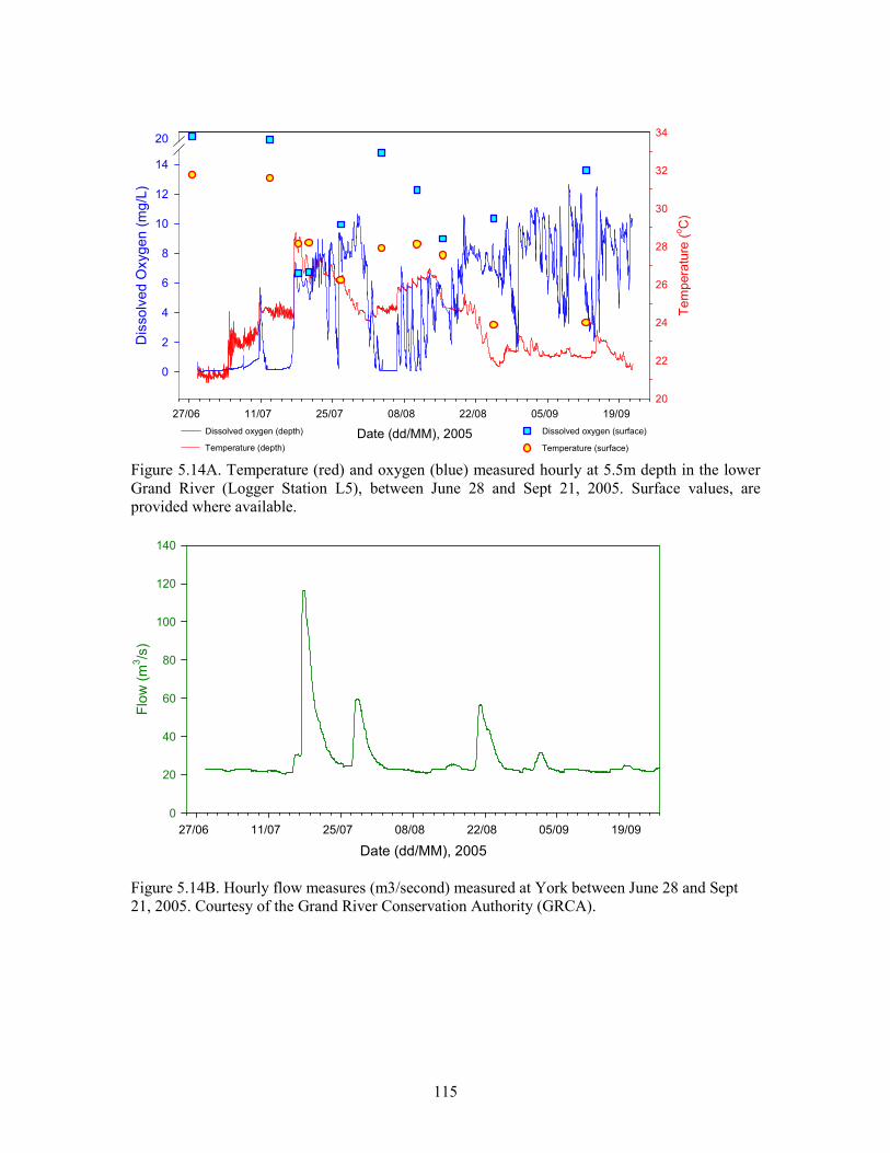
115
Date (dd/MM), 2005
27/06 11/07 25/07 08/08 22/08 05/09 19/09
Tem
pera
ture
(oC
)
20
22
24
26
28
30
32
34
Temperature (depth)
Dis
so
lve
d O
xyg
en
(m
g/L
)
0
2
4
6
8
10
12
14
20
Dissolved oxygen (depth) Dissolved oxygen (surface)
Temperature (surface)
Figure 5.14A. Temperature (red) and oxygen (blue) measured hourly at 5.5m depth in the lower
Grand River (Logger Station L5), between June 28 and Sept 21, 2005. Surface values, are
provided where available.
Date (dd/MM), 2005
27/06 11/07 25/07 08/08 22/08 05/09 19/09
Flo
w (
m3/s
)
0
20
40
60
80
100
120
140
Figure 5.14B. Hourly flow measures (m3/second) measured at York between June 28 and Sept
21, 2005. Courtesy of the Grand River Conservation Authority (GRCA).

116
Date (dd/MM), 2005
27/06 01/07 05/07 09/07 13/07 17/07 21/07
Tem
pera
ture
(oC
)
20
22
24
26
28
30
32
34
Temperature (depth)
Dis
so
lve
d O
xyg
en
(m
g/L
) A
ND
Flo
w (
x 1
0 m
3/L
)
0
2
4
6
8
10
12
14
20
Dissolved oxygen (depth) Dissolved oxygen (surface)
Temperature (surface)
Flow at York
Figure 5.14C. Temperature (red) and oxygen (blue) measured hourly at 5.5m depth in the lower Grand
River (Logger Station L5), between June 28 and July 21, 2005. Surface values, are provided where
available. The green line indicates river flow measured at York (courtesy of GRCA)
Date (dd/MM), 2005
20/07 22/07 24/07 26/07 28/07
06:
00 1
2:00
18:
00 0
0:00
06:
00 1
2:00
18:
00
06:
00 1
2:00
18:
00 0
0:00
06:
00 1
2:00
18:
00
06:
00 1
2:00
18:
00 0
0:00
06:
00 1
2:00
18:
00
06:
00 1
2:00
18:
00 0
0:00
06:
00 1
2:00
18:
00
Te
mpe
ratu
re (
oC
)
20
22
24
26
28
30
32
34
Temperature (depth)
Dis
so
lve
d O
xyg
en
(m
g/L
) A
ND
Flo
w (
x 1
0 m
3/L
)
0
2
4
6
8
10
12
14
20
Dissolved oxygen (depth) Dissolved oxygen (surface)
Temperature (surface)
Flow at York
Figure 5.14D. Temperature (red) and oxygen (blue) measured hourly at 5.5m depth in the lower Grand
River (Logger Station L5), between July 20 and July 28, 2005. Surface values, are provided where
available. The green line indicates river flow measured at York (courtesy of GRCA)

117
Date (dd/MM), 2005
28/07 30/07 01/08 03/08 05/08 07/08
06:
00 1
2:00
18:
00 0
0:00
06:
00 1
2:00
18:
00
06:
00 1
2:00
18:
00 0
0:00
06:
00 1
2:00
18:
00
06:
00 1
2:00
18:
00 0
0:00
06:
00 1
2:00
18:
00
06:
00 1
2:00
18:
00 0
0:00
06:
00 1
2:00
18:
00
06:
00 1
2:00
18:
00 0
0:00
06:
00 1
2:00
18:
00
06:
00 1
2:00
18:
00 0
0:00
Te
mpe
ratu
re (
oC
)
20
22
24
26
28
30
32
34
Temperature (depth)
Dis
so
lve
d O
xyg
en
(m
g/L
) A
ND
Flo
w (
x1
0 m
3/L
)
0
2
4
6
8
10
12
14
20
Dissolved oxygen (depth) Dissolved oxygen (surface)
Temperature (surface)
Flow at York
Figure 5.14E. Temperature (red) and oxygen (blue) measured hourly at 5.5m depth in the lower
Grand River (Logger Station L5), between July 28 and Aug 8, 2005. Surface values, are provided
where available. The green line indicates river flow measured at York (courtesy of GRCA)
Date (dd/MM), 2005
08/08 10/08 12/08 14/08 16/08 18/08 20/08 22/08 24/08
06:
00 1
2:00
18:
00 0
0:00
06:
00 1
2:00
18:
00 0
6:00
12:
00 1
8:00
00:
00 0
6:00
12:
00 1
8:00
06:
00 1
2:00
18:
00 0
0:00
06:
00 1
2:00
18:
00 0
6:00
12:
00 1
8:00
00:
00 0
6:00
12:
00 1
8:00
06:
00 1
2:00
18:
00 0
0:00
06:
00 1
2:00
18:
00 0
6:00
12:
00 1
8:00
00:
00 0
6:00
12:
00 1
8:00
06:
00 1
2:00
18:
00 0
0:00
06:
00 1
2:00
18:
00 0
6:00
12:
00 1
8:00
00:
00 0
6:00
12:
00 1
8:00
Te
mpe
ratu
re (
oC
)
20
22
24
26
28
30
32
34
Temperature (depth)
Dis
so
lve
d O
xyg
en
(m
g/L
) A
ND
Flo
w (
x1
0 m
3/L
)
0
2
4
6
8
10
12
14
20
Dissolved oxygen (depth) Dissolved oxygen (surface)
Temperature (surface)
Flow at York
Figure 5.14F. Temperature (red) and oxygen (blue) measured hourly at 5.5m depth in the lower
Grand River (Logger Station L5), between Aug 8 and Aug 25, 2005. Surface values, are provided
where available. The green line indicates river flow measured at York (courtesy of GRCA)

118
Date (dd/MM), 2005
24/08 26/08 28/08 30/08 01/09 03/09
06:
00 1
2:00
18:
00 0
0:00
06:
00 1
2:00
18:
00
06:
00 1
2:00
18:
00 0
0:00
06:
00 1
2:00
18:
00
06:
00 1
2:00
18:
00 0
0:00
06:
00 1
2:00
18:
00
06:
00 1
2:00
18:
00 0
0:00
06:
00 1
2:00
18:
00
06:
00 1
2:00
18:
00 0
0:00
06:
00 1
2:00
18:
00
Te
mpe
ratu
re (
oC
)
20
22
24
26
28
30
32
34
Temperature (depth)
Dis
so
lve
d O
xyge
n (
mg/L
) A
ND
Flo
w (
x1
0 m
3/L
)
0
2
4
6
8
10
12
14
20
Dissolved oxygen (depth) Dissolved oxygen (surface)
Temperature (surface)
Flow at York
Figure 5.14G. Temperature (red) and oxygen (blue) measured hourly at 5.5m depth in the lower
Grand River (Logger Station L5), between Aug 24 and Sep 04, 2005. Surface values, are
provided where available. The green line indicates river flow measured at York (courtesy of
GRCA)
Date (dd/MM), 2005
03/09 05/09 07/09 09/09 11/09
06:
00 1
2:00
18:
00 0
0:00
06:
00 1
2:00
18:
00
06:
00 1
2:00
18:
00 0
0:00
06:
00 1
2:00
18:
00
06:
00 1
2:00
18:
00 0
0:00
06:
00 1
2:00
18:
00
06:
00 1
2:00
18:
00 0
0:00
06:
00 1
2:00
18:
00
06:
00 1
2:00
18:
00 0
0:00
Tem
pe
ratu
re (
oC
)
20
22
24
26
28
30
32
34
Temperature (depth)
Dis
so
lve
d O
xyge
n (
mg/L
) A
ND
Flo
w (
x 1
0 m
3/L
)
0
2
4
6
8
10
12
14
20
Dissolved oxygen (depth) Dissolved oxygen (surface)
Temperature (surface)
Flow at York
Figure 5.14H. Temperature (red) and oxygen (blue) measured hourly at 5.5m depth in the lower
Grand River (Logger Station L5), between Sept 03 and Sept 12, 2005. Surface values, are
provided where available. The green line indicates river flow measured at York (courtesy of
GRCA)

119
Date (dd/MM), 2005
12/09 14/09 16/09 18/09 20/09
06:
00 1
2:00
18:
00 0
0:00
06:
00 1
2:00
18:
00
06:
00 1
2:00
18:
00 0
0:00
06:
00 1
2:00
18:
00
06:
00 1
2:00
18:
00 0
0:00
06:
00 1
2:00
18:
00
06:
00 1
2:00
18:
00 0
0:00
06:
00 1
2:00
18:
00
06:
00 1
2:00
18:
00 0
0:00
Tem
pe
ratu
re (
oC
)
20
22
24
26
28
30
32
34
Temperature (depth)
Dis
so
lved O
xygen (
mg/L
) A
ND
Flo
w (
x 1
0 m
3/L
)
0
2
4
6
8
10
12
14
20
Dissolved oxygen (depth) Dissolved oxygen (surface)
Temperature (surface)
Flow at York
Figure 5.14I. Temperature (red) and oxygen (blue) measured hourly at 5.5m depth in the lower
Grand River (Logger Station L5), between Sept 12 and Sept 28, 2005. Surface values, are
provided where available. The green line indicates river flow measured at York (courtesy of
GRCA)

120
5.7 Tables

121
Table 5.1. Temperature logging station details, Grand River, 2001-2005
Station IDRelative to
Dunnville Dam
Relative to
Main channelDepth Longitude Longitude General Description
(m) (decimal degrees) (decimal degrees)
T1 Below Main 1.6 42.8620 -79.5760 Port Maitland
T2 Below Main 1.5 42.8997 -79.6157 Riverside Marina; Dunnville (below dam)
T3 Below Main 1.2 42.8970 -79.6291 Fishway; Dunnville (below dam)
T4 Above Main 1.0 42.8974 -79.6287 Fishway; Dunnville (above dam)
T5 Above Main 1.0 42.9152 -79.6541 R.C. residence; Dunnville (approx 1km above dam))
T6w Above Main 0.5 42.9385 -79.8534 Cayuga (fall, winter, spring)
T6s Above Main 1.2 42.9456 -79.8611 Cayuga (summer)
T7 Above Tributary 1.5 42.9765 -79.8846 Rogers Ck (just upstream of confluence with GR main channel)
T8 Above Main 0.5 43.0106 -79.8798 York
T9 Above Tributary 0.3 43.0190 -79.8975 Boston-MacKenzie Ck (just upstream of concluence with GR main channel)
T10 Above Main 0.5 43.0577 -79.9187 Caledonia
TQ1 Above Tributary 0.3 42.9461 -79.9147 Mill Creek at Decewsville Rd.(above old Taquanya resevoir)
TQ2 Above Tributary 0.5 42.9558 -79.9131 Mill Creek at Townline Rd.(below old Taquanya resevoir)
TQ3 Above Tributary 0.2 42.9703 -79.8987 Mill Creek at R. Fox property
TQ4 Above Tributary 1.0 42.9785 -79.8975 Rogers Creek at Indianna Rd. (upstream of confluence with Mill Ck.)

122
Table 5.2. Duration of temperature logging and frequency of measurements (1-2 /hr) at 10
stations, Grand River, 2001-2005.
TL1 TL2 TL3 TL4 TL5 TL6 TL7 TL8 TL9 TL10
Port M. Riverside Downstream Upstream Culps Cayuga Rogers C. York Boston M. Caledonia
Jan
Feb
Mar
Apr
May
Jun
Jul
Aug
Sep
Oct
Nov
Dec 2 hr 2 hr
Jan
Feb
Mar
Apr
May
Jun
Jul
Aug
Sep
Oct
Nov
Dec
Jan
Feb 2 hr 2 hr
Mar
Apr
May 1 hr 1 hr
Jun
Jul
Aug
Sep 1 hr 1 hr 1 hr 1 hr 1 hr
Oct
Nov
Dec
Jan
Feb
Mar
Apr 1 hr 1 hr 2 hr 2 hr 2 hr 2 hr 2 hr
May
Jun 2 hr 2 hr
Jul
Aug
Sep
Oct 2 hr 2 hr
Nov
Dec
Jan
Feb 2 hr
Mar
Apr
May 1 hr 1 hr
Jun
Jul 2 hr 2 hr 2 hr 2 hr 2 hr
Aug 2 hr 2 hr
Sep
Oct
Nov
Dec
2005
2001
2002
2003
2004

123
Table 5.3. Temperature and oxygen profiling: frequency of sampling events at 10 stations within
the Grand River between 2003 and 2005.
YearSample
DatesTO-1 TO-2 TO-3 TO-4 TO-5 TO-6 TO-7 TO-8 TO-9 TO-10
09-Jul
13-Aug
25-Aug
09-Sep
23-Sep
07-Oct
21-Oct
15-Jun
23-Jun
29-Jun
06-Jul
13-Jul
20-Jul
26-Jul
03-Aug
09-Aug
23-Aug
30-Aug
10-Sep
23-Sep
05-Oct
10-Oct
20-Oct
15-Jun
27-Jun
12-Jul
18-Jul
20-Jul
26-Jul
03-Aug
10-Aug
15-Aug
25-Aug
12-Sep
2004
2005
Stations
2003

124
Table 5.4. Continuous logging of temperature and oxygen at depth: station locations, descriptions and duration of logging events.
Year Station ID DEPTH LAT LON Description START STOP Duration
(m) (north) (east) (days_hour:min)
2004 L1 0.75 42.91511 -79.65406 RC residence 08-Jul-04 13-Jul-04 04 19:45
2004 L2 2.0 42.90092 -79.62115 Above Dam (1) 22-Jul-04 26-Jul-04 03 21:00
Above Dam (2) 29-Jul-04 30-Jul-04 04 22:30
Above Dam (3) 26-Aug-04 30-Aug-04 03 23:00
Above Dam (4) 01-Sep-04 10-Sep-04 08 23:30
2004 L3 3.8 42.91724 -79.74079 RV resort 29-Jul-04 12-Aug-04 14 1:00
2004 L4 1.0 42.89585 -79.62913 Sulphur Ck. 12-Aug-04 23-Aug-04 10 21:30
2005 L5 6.5 42.92720 -79.68040 Breakwall (profile stn6) 28-Jun-05 21-Sep-05 85 00:00

125
Table 5.5. Summary of temperature and oxygen profile data, Grand River, 2003
Station ID Date
yy-mm-dd Max ∆D Max Min ∆T Max Min ∆ % Max Min ∆DO
4 03-07-09 2.5 2.0 28.52 26.05 -2.47 144.0 57.0 -87.0 11.14 4.61 -6.53
5 03-07-09 3.5 3.0 27.56 25.75 -1.81 170.7 59.4 -111.3 13.45 4.83 -8.62
6 03-07-09 6.5 5.5 27.84 25.77 -2.07 196.3 63.2 -133.1 15.44 5.14 -10.30
7 03-07-09 5.0 5.0 27.27 24.57 -2.70 236.4 5.9 -230.5 19.69 0.49 -19.20
4 03-08-13 1.5 1.0 27.04 25.29 -1.75 139.6 98.9 -40.7 11.22 8.21 -3.01
5 03-08-13 3.5 3.5 25.05 24.86 -0.19 100.3 87.7 -12.6 8.23 7.37 -0.86
6 03-08-13 6.0 5.5 25.61 24.86 -0.75 136.6 94.5 -42.1 11.33 7.91 -3.42
7 03-08-13 5.0 4.0 24.57 24.46 -0.11 96.0 85.3 -10.7 8.08 7.19 -0.89
8 03-08-13 4.0 4.0 28.09 25.45 -2.64 165.2 110.7 -54.5 13.03 9.09 -3.94
9 03-08-13 4.0 3.0 25.52 24.27 -1.25 100.6 83.4 -17.2 8.32 7.05 -1.27
4 03-08-25 2.0 1.5 24.57 24.15 -0.42 110.8 99.2 -11.6 9.19 8.30 -0.89
5 03-08-25 2.5 2.5 25.20 24.17 -1.03 131.5 97.1 -34.4 10.79 8.11 -2.68
6 03-08-25 6.0 6.0 25.54 24.43 -1.11 142.4 88.0 -54.4 11.61 7.32 -4.29
7 03-08-25 5.0 5.0 26.59 24.58 -2.01 141.9 81.0 -61.0 11.45 6.72 -4.73
8 03-08-25 3.0 3.0 24.99 23.74 -1.25 143.2 103.0 -40.2 11.79 8.68 -3.11
9 03-08-25 4.0 4.0 24.17 22.97 -1.20 139.2 91.9 -47.3 11.63 7.85 -3.78
4 03-09-09 1.5 1.0 22.78 21.78 -1.00 9.15 8.15 -1.00
5 03-09-09 3.0 3.0 22.36 20.63 -1.73 8.95 5.99 -2.96
6 03-09-09 5.5 5.5 22.11 21.23 -0.88 8.71 6.53 -2.18
7 03-09-09 5.0 5.0 22.00 21.01 -0.99 9.48 6.98 -2.50
8 03-09-09 3.5 3.5 22.83 21.85 -0.98 10.76 8.22 -2.54
9 03-09-09 4.0 4.0 23.64 21.51 -2.13 11.38 7.41 -3.97
4 03-09-23 2.0 1.5 18.52 18.40 -0.12 68.8 65.2 -3.6 6.38 6.07 -0.31
5 03-09-23 3.5 3.5 18.56 10.81 -7.75 84.7 62.6 -22.1 9.43 5.84 -3.59
6 03-09-23 4.5 4.5 18.66 18.62 -0.04 75.7 72.7 -3.0 7.01 6.73 -0.28
7 03-09-23 3.5 3.5 18.75 18.71 -0.04 68.7 65.6 -3.1 6.35 6.06 -0.29
8 03-09-23 2.0 2.0 18.77 18.75 -0.02 68.7 67.7 -1.0 6.35 6.25 -0.10
9 03-09-23 4.0 4.0 17.93 17.89 -0.04 66.1 63.6 -2.5 6.21 5.98 -0.23
4 03-10-07 2.0 1.5 11.71 11.61 -0.10 96.2 94.1 -2.1 10.49 10.28 -0.21
5 03-10-07 3.0 3.0 11.68 10.78 -0.90 94.8 83.3 -11.5 10.27 9.27 -1.00
6 03-10-07 6.0 6.0 11.87 10.82 -1.05 93.5 84.6 -8.9 10.15 9.43 -0.72
7 03-10-07 5.0 5.0 11.56 10.50 -1.06 97.1 87.8 -9.3 10.62 9.84 -0.78
8 03-10-07 3.0 3.0 11.60 10.89 -0.71 101.7 96.1 -5.7 11.12 10.67 -0.45
9 03-10-07 4.0 4.0 11.29 10.81 -0.48 90.6 86.8 -3.8 9.98 9.66 -0.32
4 03-10-21 1.5 1.0 10.82 10.81 -0.01 77.6 75.3 -2.3 8.45 8.20 -0.25
5 03-10-21 3.0 3.0 10.37 10.36 -0.01 71.3 68.7 -2.6 8.12 7.56 -0.56
6 03-10-21 6.5 6.5 10.28 10.27 -0.01 77.3 71.5 -5.8 8.53 7.89 -0.64
7 03-10-21 6.0 6.0 10.84 10.12 -0.72 84.8 78.8 -6.0 9.44 8.72 -0.72
8 03-10-21 4.0 4.0 10.77 10.76 -0.01 94.7 91.2 -3.5 10.33 9.94 -0.39
9 03-10-21 5.0 5.0 11.32 11.29 -0.03 87.5 84.7 -2.8 9.42 9.12 -0.30
Depth Temperature Dissolved Oxygen
(oC) DO - % Saturation DO (mg/L)

126
Table 5.6. Summary of temperature and oxygen profile data, Grand River, 2004
Station Date
ID yy-mm-dd Max Min ∆D Max Min ∆T Max Min ∆ % Max Min ∆DO
5 04-06-15 3.3 0.2 3.2 24.43 21.73 -2.70 155.4 102.1 -53.3 12.95 8.95 -4.00
6 04-06-15 5.7 0.2 5.5 24.19 21.90 -2.29 173.4 103.3 -70.1 14.63 9.02 -5.61
7 04-06-15 4.3 0.2 4.2 25.49 21.99 -3.50 180.1 113.0 -67.1 14.79 9.86 -4.93
8 04-06-15 3.9 0.2 3.8 26.30 22.02 -4.28 195.5 98.0 -97.5 15.79 8.55 -7.24
9 04-06-15 3.4 0.2 3.2 24.35 23.10 -1.25 145.6 101.3 -44.3 12.15 8.65 -3.50
10 04-06-15 1.4 0.2 1.2 24.86 24.83 -0.03 164.1 163.2 -0.9 13.57 13.49 -0.08
1 04-06-23 6.0 0.2 5.8 21.56 18.28 -3.28 100.6 81.3 -19.3 8.85 7.40 -1.45
2 04-06-23 4.5 0.2 4.4 22.72 20.65 -2.07 126.2 83.8 -42.4 10.88 7.51 -3.37
3 04-06-23 4.0 0.2 3.8 22.06 20.63 -1.43 109.9 87.9 -22.0 9.58 7.88 -1.70
5 04-06-23 3.6 0.2 3.5 22.30 20.35 -1.95 115.7 84.0 -31.7 10.04 7.57 -2.47
6 04-06-23 6.0 0.2 5.9 13.37 21.37 8.00 127.9 94.6 -33.3 10.88 8.36 -2.52
7 04-06-23 5.0 0.2 4.9 22.38 20.36 -2.02 112.9 77.2 -35.7 9.78 6.95 -2.83
8 04-06-23 4.0 0.2 3.9 22.95 21.42 -1.53 118.7 101.8 -16.9 10.17 8.98 -1.19
9 04-06-23 3.5 0.2 3.3 22.13 20.20 -1.93 103.8 84.2 -19.6 9.03 7.61 -1.42
10 04-06-23 2.0 0.2 1.9 22.52 22.50 -0.02 120.1 118.8 -1.3 10.38 10.27 -0.11
1 04-06-29 5.8 0.2 5.6 20.36 20.19 -0.17 93.3 87.5 -5.8 8.40 7.91 -0.49
2 04-06-29 4.5 0.2 4.4 10.39 19.98 9.59 96.8 88.9 -7.9 8.72 8.07 -0.65
3 04-06-29 3.0 0.2 2.9 20.07 20.04 -0.03 99.5 97.7 -1.8 9.02 8.86 -0.16
5 04-06-29 3.5 0.2 3.3 20.66 20.31 -0.35 109.7 107.2 -2.5 9.83 9.67 -0.16
6 04-06-29 4.7 0.2 4.5 21.09 20.53 -0.56 103.0 95.5 -7.5 9.15 8.58 -0.57
8 04-06-29 3.5 0.2 3.4 19.98 19.39 -0.59 86.5 77.6 -8.9 7.85 7.12 -0.73
9 04-06-29 3.5 0.2 3.3 20.50 19.63 -0.87 104.8 96.4 -8.4 9.42 8.81 -0.61
10 04-06-29 2.0 0.2 1.9 20.79 20.75 -0.04 105.8 105.1 -0.7 9.45 9.39 -0.06
1 04-07-06 6.0 0.2 5.8 23.58 21.56 -2.02 89.9 78.3 -11.6 7.61 6.76 -0.85
2 04-07-06 4.5 0.2 4.3 23.44 23.15 -0.29 101.7 83.3 -18.4 8.63 7.11 -1.52
3 04-07-06 4.0 0.2 3.9 23.60 22.94 -0.66 104.4 83.2 -21.2 8.83 7.13 -1.70
5 04-07-06 3.0 0.2 2.8 24.61 22.94 -1.67 151.3 88.8 -62.5 12.59 7.61 -4.98
6 04-07-06 6.0 0.2 5.8 24.95 23.04 -1.91 179.3 86.2 -93.1 14.95 7.37 -7.58
7 04-07-06 5.0 0.2 4.9 25.30 23.00 -2.30 182.5 88.3 -94.2 15.03 7.56 -7.47
8 04-07-06 4.0 0.2 3.9 25.83 22.75 -3.08 164.5 91.8 -72.7 13.85 7.89 -5.96
9 04-07-06 3.5 0.1 3.4 25.36 22.65 -2.71 177.2 99.8 -77.4 14.67 8.60 -6.07
10 04-07-06 1.5 0.1 1.3 24.56 24.49 -0.07 113.6 113.1 -0.5 9.45 9.41 -0.04
1 04-07-13 6.0 0.1 5.9 25.19 22.79 -2.40 158.4 42.5 -115.9 13.01 3.62 -9.39
2 04-07-13 4.5 0.1 4.4 24.94 24.04 -0.90 127.7 69.0 -58.7 10.54 5.79 -4.75
3 04-07-13 4.0 0.1 3.9 24.96 24.24 -0.72 150.9 84.5 -66.4 12.45 7.06 -5.39
5 04-07-13 3.5 0.1 3.4 25.58 22.54 -3.04 192.8 49.4 -143.4 15.73 4.26 -11.47
6 04-07-13 6.0 0.1 5.9 27.31 22.89 -4.42 289.9 60.3 -229.6 22.93 5.17 -17.76
7 04-07-13 5.0 0.1 5.0 26.38 22.40 -3.98 155.9 41.6 -114.3 12.54 3.61 -8.93
8 04-07-13 4.0 0.1 3.9 27.00 22.62 -4.38 147.8 66.9 -80.9 11.79 5.77 -6.02
9 04-07-13 4.5 0.1 4.4 26.16 22.79 -3.37 112.5 67.9 -44.6 9.08 5.83 -3.25
10 04-07-13 2.1 0.1 2.0 25.71 25.68 -0.03 109.9 107.0 -2.9 8.95 8.71 -0.24
1 04-07-20 6.0 0.1 5.9 23.39 22.78 -0.61 104.4 79.8 -24.6 8.87 6.84 -2.03
2 04-07-20 4.5 0.1 4.4 23.96 22.71 -1.25 115.5 50.6 -64.9 9.71 4.35 -5.36
3 04-07-20 4.0 0.1 3.9 23.58 22.93 -0.65 109.5 80.1 -29.4 9.27 6.86 -2.41
5 04-07-20 3.5 0.1 3.4 24.55 23.15 -1.40 112.6 86.7 -25.9 9.37 7.40 -1.97
6 04-07-20 6.1 0.1 5.9 24.43 23.25 -1.18 94.0 76.2 -17.8 7.83 6.49 -1.34
7 04-07-20 5.0 0.1 4.9 24.42 23.23 -1.19 92.3 77.9 -14.4 7.70 6.64 -1.06
8 04-07-20 4.1 0.1 3.9 25.20 24.10 -1.10 102.0 88.3 -13.7 8.38 7.40 -0.98
9 04-07-20 4.5 0.1 4.4 24.40 23.14 -1.26 91.4 74.9 -16.5 7.62 6.39 -1.23
10 04-07-20 2.0 0.1 1.9 25.29 25.23 -0.06 102.6 101.0 -1.6 8.41 8.29 -0.12
1 04-07-26 6.0 0.2 5.8 22.81 22.96 0.15 96.1 91.5 -4.6 8.26 7.86 -0.40
2 04-07-26 4.5 0.2 4.3 22.91 22.89 -0.02 103.4 98.3 -5.1 8.87 8.43 -0.44
3 04-07-26 4.1 0.2 3.9 22.82 22.66 -0.16 101.2 90.3 -10.9 8.70 7.78 -0.92
5 04-07-26 3.5 0.2 3.3 23.00 22.95 -0.05 103.6 92.0 -11.6 8.87 7.88 -0.99
6 04-07-26 6.1 0.2 5.9 23.01 22.90 -0.11 108.5 103.0 -5.5 8.29 8.84 0.55
7 04-07-26 5.0 0.2 4.8 23.18 23.00 -0.18 119.5 101.0 -18.5 10.20 8.65 -1.55
8 04-07-26 4.0 0.2 3.8 22.27 22.24 -0.03 87.3 87.0 -0.3 7.58 7.55 -0.03
9 04-07-26 4.5 0.2 4.3 23.21 23.18 -0.03 103.3 102.7 -0.6 8.81 8.75 -0.06
10 04-07-26 2.0 0.2 1.8 21.95 21.88 -0.07 90.3 88.9 -1.4 7.90 7.77 -0.13
Depth Temperature Dissolved Oxygen
(oC) DO - % Saturation DO (mg/L)
(cont’d)

127
Table 5.6 (cont’d). Summary of temperature and oxygen profile data, Grand River, 2004
Station Date
ID yy-mm-dd Max Min ∆D Max Min ∆T Max Min ∆ % Max Min ∆DO
1 04-08-03 6.1 0.1 6.0 25.73 24.38 -1.35 119.6 86.5 -33.1 9.74 7.21 -2.53
2 04-08-03 5.0 0.1 4.9 26.23 24.42 -1.81 139.3 89.1 -50.2 11.23 7.43 -3.80
3 04-08-03 4.0 0.1 3.9 25.75 24.31 -1.44 120.6 89.2 -31.4 9.81 7.45 -2.36
5 04-08-03 3.5 0.1 3.4 25.43 24.58 -0.85 110.5 90.3 -20.2 9.04 7.50 -1.54
6 04-08-03 6.5 0.1 6.4 26.00 24.68 -1.32 117.1 88.4 -28.7 7.50 7.33 -0.17
7 04-08-03 5.0 0.1 4.9 24.95 23.75 -1.20 99.3 78.6 -20.7 8.20 6.63 -1.57
8 04-08-03 4.0 0.1 3.9 27.30 25.08 -2.22 136.1 96.9 -39.2 10.77 7.98 -2.79
9 04-08-03 5.0 0.1 4.9 26.57 24.99 -1.58 117.9 88.4 -29.5 9.45 7.30 -2.15
10 04-08-03 2.1 0.1 2.0 25.69 25.59 -0.10 108.0 106.6 -1.4 8.82 8.68 -0.14
1 04-08-09 6.1 0.2 5.9 22.80 22.14 -0.66 129.5 101.4 -28.1 11.14 8.83 -2.31
2 04-08-09 4.5 0.2 4.3 23.41 21.88 -1.53 149.9 95.3 -54.6 12.76 8.34 -4.42
3 04-08-09 4.0 0.2 3.8 23.35 22.33 -1.02 136.7 81.3 -55.4 11.64 7.05 -4.59
5 04-08-09 3.5 0.2 3.3 23.61 21.91 -1.70 178.4 118.1 -60.3 15.10 10.32 -4.78
6 04-08-09 6.5 0.2 6.3 24.02 21.85 -2.17 208.6 130.7 -77.9 17.52 11.44 -6.08
7 04-08-09 5.0 0.2 4.8 23.47 21.59 -1.88 198.3 97.7 -100.6 16.83 8.60 -8.23
8 04-08-09 3.5 0.2 3.4 24.71 21.70 -3.01 223.5 122.0 -101.5 18.53 10.70 -7.83
9 04-08-09 4.5 0.2 4.3 24.85 21.50 -3.35 190.0 114.6 -75.4 15.72 10.10 -5.62
10 04-08-09 2.0 0.2 1.8 22.71 22.68 -0.03 127.1 126.0 -1.1 10.94 10.85 -0.09
1 04-08-23 6.1 0.2 5.9 21.94 21.42 -0.52 119.4 103.8 -15.6 10.44 9.16 -1.28
2 04-08-23 4.5 0.2 4.4 22.47 21.08 -1.39 139.5 79.0 -60.5 72.06 7.02 -65.04
3 04-08-23 4.0 0.2 3.9 22.42 21.55 -0.87 119.3 88.1 -31.2 10.33 7.75 -2.58
5 04-08-23 3.5 0.1 3.4 21.76 21.51 -0.25 114.4 105.8 -8.6 10.03 9.32 -0.71
6 04-08-23 6.1 0.2 5.9 21.81 21.44 -0.37 117.4 105.3 -12.1 10.28 9.29 -0.99
7 04-08-23 5.0 0.2 4.9 21.29 20.86 -0.43 119.6 108.6 -11.0 10.60 9.68 -0.92
8 04-08-23 3.5 0.1 3.4 21.52 21.35 -0.17 123.9 120.0 -3.9 10.91 10.60 -0.31
9 04-08-23 4.5 0.2 4.4 21.05 20.10 -0.95 116.8 74.3 -42.5 10.38 6.72 -3.66
10 04-08-23 2.0 0.2 1.9 20.80 20.71 -0.09 98.0 96.7 -1.3 8.75 8.64 -0.11
1 04-08-30 6.0 0.2 5.8 22.70 22.52 -0.18 86.2 79.0 -7.2 7.42 6.83 -0.59
2 04-08-30 4.5 0.2 4.3 22.65 22.31 -0.34 90.4 80.3 -10.1 7.79 6.96 -0.83
3 04-08-30 4.0 0.2 3.8 22.59 22.21 -0.38 89.7 83.4 -6.3 7.78 7.25 -0.53
5 04-08-30 3.5 0.2 3.4 22.50 22.40 -0.10 88.3 83.3 -5.0 7.63 7.21 -0.42
6 04-08-30 6.5 0.2 6.3 22.63 22.59 -0.04 84.9 83.4 -1.5 7.32 7.19 -0.13
7 04-08-30 5.0 0.2 4.8 22.46 22.44 -0.02 88.7 87.7 -1.0 7.67 7.58 -0.09
8 04-08-30 4.0 0.2 3.8 22.51 22.44 -0.07 90.7 89.1 -1.6 7.84 7.71 -0.13
9 04-08-30 4.5 0.2 4.3 22.28 22.26 -0.02 79.0 78.0 -1.0 6.85 6.77 -0.08
10 04-08-30 2.0 0.2 1.8 22.04 22.00 -0.04 79.6 79.4 -0.2 6.94 6.92 -0.02
1 04-09-10 6.0 0.2 5.8 21.90 19.28 -2.62 108.7 68.2 -40.5 9.51 6.29 -3.22
2 04-09-10 4.5 0.2 4.3 22.61 20.19 -2.42 130.2 79.7 -50.5 11.23 7.21 -4.02
3 04-09-10 4.0 0.2 3.8 21.74 19.93 -1.81 102.7 77.6 -25.1 9.01 7.05 -1.96
5 04-09-10 3.5 0.2 3.3 21.03 20.40 -0.63 79.6 72.8 -6.8 7.08 6.56 -0.52
6 04-09-10 6.5 0.2 6.3 21.49 20.29 -1.20 85.7 71.9 -13.8 7.64 6.48 -1.16
7 04-09-10 5.0 0.2 4.8 22.07 20.13 -1.94 91.6 73.1 -18.5 8.01 6.62 -1.39
8 04-09-10 3.5 0.2 3.3 21.52 19.59 -1.93 100.9 82.3 -18.6 8.88 7.51 -1.37
9 04-09-10 4.5 0.2 4.3 22.19 20.58 -1.61 108.4 93.1 -15.3 9.47 8.35 -1.12
10 04-09-10 2.0 0.2 1.8 21.35 21.32 -0.03 99.2 96.1 -3.1 8.77 8.50 -0.27
1 04-09-23 6.1 0.3 5.8 20.71 19.33 -1.38 135.5 62.1 -73.4 12.13 5.71 -6.42
2 04-09-23 4.5 0.3 4.3 20.37 19.14 -1.23 113.7 65.4 -48.3 10.24 6.03 -4.21
3 04-09-23 4.0 0.3 3.7 20.97 19.45 -1.52 117.7 55.2 -62.5 10.48 5.07 -5.41
5 04-09-23 3.5 0.3 3.3 22.02 18.70 -3.32 149.6 89.1 -60.5 13.46 8.29 -5.17
6 04-09-23 6.0 0.3 5.8 21.53 19.10 -2.43 154.9 108.2 -46.7 13.98 10.00 -3.98
7 04-09-23 5.0 0.3 4.8 21.93 18.32 -3.61 139.1 46.6 -92.5 12.25 4.37 -7.88
8 04-09-23 3.5 0.2 3.3 22.54 18.39 -4.15 153.4 89.1 -64.3 13.43 8.35 -5.08
9 04-09-23 4.5 0.3 4.3 23.13 17.84 -5.29 169.2 50.6 -118.6 14.81 4.80 -10.01
10 04-09-23 2.0 0.2 1.8 20.55 19.84 -0.71 124.0 13.7 -110.3 11.28 10.20 -1.08
1 04-10-05 5.8 0.3 5.6 16.06 15.15 -0.91 106.2 81.3 -24.9 10.44 8.15 -2.29
2 04-10-05 4.5 0.3 4.3 16.53 15.14 -1.39 115.1 85.4 -29.7 11.20 8.57 -2.63
3 04-10-05 4.0 0.3 3.8 15.72 15.08 -0.64 100.0 79.3 -20.7 9.91 7.96 -1.95
5 04-10-05 3.5 0.3 3.3 16.38 15.21 -1.17 100.4 80.8 -19.6 9.81 8.09 -1.72
6 04-10-05 6.5 0.3 6.2 16.69 15.73 -0.96 96.5 83.0 -13.5 9.37 8.21 -1.16
7 04-10-05 5.0 0.3 4.7 16.57 15.86 -0.71 101.6 87.5 -14.1 9.91 8.64 -1.27
8 04-10-05 3.5 0.3 3.2 15.20 14.46 -0.74 103.3 91.4 -11.9 10.36 9.30 -1.06
9 04-10-05 4.5 0.3 4.2 15.31 14.77 -0.54 89.7 85.8 -3.9 9.00 8.67 -0.33
10 04-10-05 2.0 0.3 1.7 13.03 12.81 -0.22 82.5 81.1 -1.4 8.67 8.56 -0.11
1 04-10-10 6.0 0.2 5.8 9.83 9.75 -0.08 93.9 91.7 -2.2 10.61 10.38 -0.23
2 04-10-10 4.5 0.2 4.3 10.02 9.98 -0.04 94.0 93.0 -1.0 10.57 10.47 -0.10
3 04-10-10 4.0 0.2 3.8 10.05 9.99 -0.06 93.6 92.2 -1.4 10.52 10.37 -0.15
5 04-10-20 3.5 0.2 3.3 10.10 10.08 -0.02 89.0 88.1 -0.9 9.99 9.89 -0.10
6 04-10-20 6.5 0.2 6.3 9.82 9.73 -0.09 88.7 86.6 -2.1 10.03 9.81 -0.22
7 04-10-20 5.0 0.2 4.8 9.67 9.60 -0.07 90.9 89.0 -1.9 10.32 10.11 -0.21
8 04-10-20 4.0 0.2 3.8 10.11 10.10 -0.01 89.8 89.5 -0.3 10.08 10.05 -0.03
9 04-10-20 4.0 0.2 3.8 9.62 9.59 -0.03 87.9 86.6 -1.3 9.99 9.83 -0.16
10 04-10-20 2.0 0.2 1.8 9.53 9.51 -0.02 91.7 91.1 -0.6 10.44 10.36 -0.08
Depth Temperature Dissolved Oxygen
(oC) DO - % Saturation DO (mg/L)

128
Table 5.7. Summary of temperature and oxygen profile data, Grand River, 2005.
Station Date
ID yy-mm-dd Max Min ∆D Max Min ∆T Max Min ∆ % Max Min ∆DO
1 05-06-15 6.1 0.0 6.1 26.30 22.05 -4.25 85.9 56.3 -29.6 6.91 4.91 -2.00
2 05-06-15 4.5 0.0 4.5 26.49 21.30 -5.19 84.2 2.9 -81.3 6.76 0.26 -6.50
3 05-06-15 3.9 0.0 3.9 26.38 26.22 -0.16 81.2 78.7 -2.5 6.54 6.33 -0.21
4 05-06-15 0.0 0.0 0.0 26.70 26.70 0.00 90.4 90.4 0.0 7.22 7.22 0.00
5 05-06-15 0.0 0.0 0.0 26.64 26.64 0.00 83.0 82.9 -0.1 6.64 6.64 0.00
6 05-06-15 6.1 0.0 6.1 26.76 19.32 -7.44 87.3 1.6 -85.7 6.97 0.15 -6.82
7 05-06-15 5.0 0.0 5.0 26.77 24.69 -2.08 106.9 84.6 -22.3 8.53 7.01 -1.52
8 05-06-15 4.0 0.0 4.0 26.63 20.19 -6.44 102.0 2.5 -99.5 8.16 0.23 -7.93
9 05-06-15 4.6 0.0 4.6 27.56 17.73 -9.83 111.2 1.6 -109.6 8.76 0.15 -8.61
10 05-06-15 2.0 0.0 2.0 25.99 25.70 -0.29 106.4 101.7 -4.7 8.62 8.27 -0.35
1 05-06-27 6.0 0.2 5.8 27.44 17.88 -9.56 208.8 58.7 -150.1 16.73 5.09 -11.64
2 05-06-27 5.0 0.2 4.8 28.06 19.99 -8.07 220.8 16.5 -204.3 17.45 1.50 -15.95
3 05-06-27 4.0 0.2 3.8 28.85 24.05 -4.80 266.9 12.5 -254.4 20.54 1.05 -19.49
4 05-06-27 0.6 0.2 0.4 29.36 28.18 -1.18 314.4 285.7 -28.7 24.48 21.81 -2.67
5 05-06-27 3.5 0.2 3.3 30.32 23.57 -6.75 343.0 25.1 -317.9 26.07 2.12 -23.95
6 05-06-27 6.0 0.2 5.8 31.78 22.05 -9.73 334.5 1.6 -332.9 25.40 0.14 -25.26
7 05-06-27 5.0 0.2 4.8 29.72 22.33 -7.39 356.2 2.5 -353.7 27.57 0.22 -27.35
8 05-06-27 3.5 0.2 3.3 32.05 23.87 -8.18 262.6 22.7 -239.9 20.51 1.91 -18.60
9 05-06-27 4.5 0.2 4.3 30.96 20.47 -10.49 275.7 3.7 -272.0 20.46 0.33 -20.13
10 05-06-27 2.0 0.2 1.8 28.53 28.37 -0.16 128.3 123.2 -5.1 9.92 9.56 -0.36
1 05-07-12 6.0 0.2 5.8 27.06 22.07 -4.99 167.0 9.4 -157.6 13.26 0.82 -12.44
2 05-07-12 4.5 0.2 4.3 27.37 24.80 -2.57 164.2 46.1 -118.1 12.97 3.82 -9.15
3 05-07-12 4.0 0.2 3.8 27.26 24.51 -2.75 147.4 10.8 -136.6 11.66 0.90 -10.76
4 05-07-12 1.1 0.2 0.9 28.28 26.34 -1.94 217.1 133.0 -84.1 16.97 10.70 -6.27
5 05-07-12 3.5 0.2 3.4 29.14 25.13 -4.01 237.2 14.8 -222.4 18.16 1.22 -16.94
6 05-07-12 6.0 0.2 5.8 31.61 24.93 -6.68 268.0 1.4 -266.6 19.67 0.11 -19.56
7 05-07-12 5.0 0.2 4.8 28.91 25.02 -3.89 208.1 8.8 -199.3 16.48 0.73 -15.75
8 05-07-12 4.1 0.2 3.9 29.54 24.87 -4.67 204.8 50.8 -154.0 15.72 4.20 -11.52
9 05-07-12 4.0 0.2 3.9 29.08 23.94 -5.14 164.6 20.3 -144.3 12.61 1.71 -10.90
10 05-07-12 2.0 0.2 1.8 28.53 27.94 -0.59 104.0 90.1 -13.9 8.13 6.97 -1.16
1 05-07-18 5.6 0.1 5.4 28.16 28.14 -0.02 85.4 82.7 -2.7 6.65 6.44 -0.21
2 05-07-18 4.5 0.1 4.3 28.03 27.96 -0.07 92.9 87.1 -5.8 7.25 6.81 -0.44
3 05-07-18 4.0 0.1 3.8 27.98 27.91 -0.07 97.3 96.7 -0.6 7.60 7.56 -0.04
4 05-07-18 1.5 0.1 1.4 28.13 28.09 -0.04 90.1 89.3 -0.8 7.02 6.97 -0.05
5 05-07-18 3.6 0.1 3.4 27.95 27.87 -0.08 77.2 73.9 -3.3 6.03 5.79 -0.24
6 05-07-18 6.5 0.1 6.4 28.69 28.52 -0.17 79.1 76.3 -2.8 6.10 5.91 -0.19
7 05-07-18 5.1 0.1 4.9 28.06 27.81 -0.25 84.0 77.6 -6.4 6.55 6.08 -0.47
8 05-07-18 4.0 0.1 3.9 27.26 26.76 -0.50 80.7 75.7 -5.0 6.39 6.05 -0.34
9 05-07-18 5.1 0.1 5.0 26.80 26.65 -0.15 81.0 78.3 -2.7 6.47 6.27 -0.20
10 05-07-18 2.8 0.1 2.7 27.21 27.18 -0.03 82.0 81.3 -0.7 6.50 6.45 -0.05
1 05-07-20 5.9 0.2 5.8 28.18 17.99 -10.19 86.6 68.1 -18.5 6.74 5.58 -1.16
2 05-07-20 4.5 0.2 4.3 27.78 27.03 -0.75 90.2 74.5 -15.7 7.07 5.92 -1.15
3 05-07-20 4.0 0.2 3.8 27.97 26.62 -1.35 95.9 81.5 -14.4 7.49 6.53 -0.96
4 05-07-20 1.6 0.2 1.4 28.23 26.51 -1.72 81.6 58.8 -22.8 6.35 4.72 -1.63
5 05-07-20 3.5 0.2 3.3 28.25 26.79 -1.46 84.0 64.7 -19.3 6.54 5.17 -1.37
6 05-07-20 6.5 0.2 6.3 28.00 26.16 -1.84 81.1 60.8 -20.3 6.34 4.91 -1.43
7 05-07-20 5.0 0.2 4.8 27.22 25.52 -1.70 86.2 62.4 -23.8 6.83 5.10 -1.73
8 05-07-20 4.0 0.2 3.8 29.18 27.06 -2.12 118.7 89.9 -28.8 9.09 7.15 -1.94
9 05-07-20 4.5 0.2 4.2 27.69 25.45 -2.24 96.7 69.7 -27.0 7.60 5.70 -1.90
10 05-07-20 2.0 0.2 1.8 27.64 27.46 -0.18 103.1 99.7 -3.4 8.11 7.87 -0.24
Depth Temperature Dissolved Oxygen
(oC) DO - % Saturation DO (mg/L)
(cont’d)

129
Table 5.7 (cont’d). Summary of temperature and oxygen profile data, Grand River, 2005
Station Date
ID yy-mm-dd Max Min ∆D Max Min ∆T Max Min ∆ % Max Min ∆DO
1 05-07-26 6.0 0.1 5.9 26.62 26.52 -0.10 93.8 76.5 -17.3 7.52 6.14 -1.38
2 05-07-26 4.5 0.1 4.4 26.38 26.12 -0.26 95.9 59.6 -36.3 7.72 4.82 -2.90
3 05-07-26 4.1 0.1 4.0 26.89 26.47 -0.42 93.8 85.2 -8.6 7.50 6.85 -0.65
4 05-07-26 1.5 0.1 1.4 26.70 26.64 -0.06 109.8 109.3 -0.5 8.78 8.76 -0.02
5 05-07-26 2.5 0.1 2.4 26.59 26.41 -0.18 117.2 106.9 -10.3 9.39 8.60 -0.79
6 05-07-26 5.9 0.1 5.9 26.46 26.14 -0.32 125.9 107.1 -18.8 10.11 8.65 -1.46
7 05-07-26 4.5 0.1 4.4 26.50 26.43 -0.07 123.2 117.4 -5.8 9.89 9.43 -0.46
8 05-07-26 3.5 0.1 3.4 26.19 26.04 -0.15 129.8 121.9 -7.9 10.48 9.86 -0.62
9 05-07-26 4.0 0.1 3.9 27.85 25.87 -1.98 153.2 87.4 -65.8 12.00 7.09 -4.91
10 05-07-26 1.5 0.1 1.4 26.23 26.21 -0.02 123.2 122.4 -0.8 9.94 9.88 -0.06
1 05-08-03 6.0 0.2 5.8 27.65 25.76 -1.89 125.3 33.3 -92.0 9.85 2.71 -7.14
2 05-08-03 4.5 0.2 4.3 27.54 25.54 -2.00 129.2 33.1 -96.1 10.18 2.70 -7.48
3 05-08-03 4.0 0.2 3.8 27.78 25.78 -2.00 131.6 26.2 -105.4 10.33 2.13 -8.20
4 05-08-03 1.5 0.2 1.4 27.67 26.60 -1.07 155.7 118.2 -37.5 12.24 9.47 -2.77
5 05-08-03 3.0 0.2 2.8 27.65 25.34 -2.31 181.2 39.8 -141.4 14.24 3.26 -10.98
6 05-08-03 6.5 0.2 6.4 27.91 24.96 -2.95 188.6 16.9 -171.7 14.76 1.39 -13.37
7 05-08-03 5.0 0.2 4.9 28.27 24.40 -3.87 230.6 28.6 -202.0 17.94 2.39 -15.55
8 05-08-03 4.0 0.2 3.9 28.28 24.87 -3.41 217.1 24.2 -192.9 16.88 2.00 -14.88
9 05-08-03 4.0 0.2 3.9 29.59 24.34 -5.25 225.4 41.7 -183.7 17.13 3.48 -13.65
10 05-08-03 2.0 0.2 1.8 27.88 27.79 -0.09 161.0 158.0 -3.0 12.63 12.39 -0.24
1 05-08-10 5.0 0.1 4.8 27.57 27.25 -0.32 103.3 80.0 -23.3 8.13 6.33 -1.80
2 05-08-10 4.6 0.2 4.4 27.57 26.26 -1.31 106.5 24.4 -82.1 8.38 1.97 -6.41
3 05-08-10 4.0 0.1 3.9 27.47 26.43 -1.04 92.4 31.2 -61.2 7.29 2.50 -4.79
4 05-08-10 1.0 0.2 0.8 27.55 27.54 -0.01 111.0 110.2 -0.8 8.74 8.68 -0.06
5 05-08-10 3.5 0.1 3.4 27.86 26.24 -1.62 118.3 22.0 -96.3 9.30 1.78 -7.52
6 05-08-10 6.0 0.2 5.8 28.16 26.78 -1.38 158.3 94.0 -64.3 12.33 7.50 -4.83
7 05-08-10 4.5 0.1 4.4 27.60 27.02 -0.58 133.5 105.6 -27.9 10.51 8.39 -2.12
8 05-08-10 3.5 0.1 3.4 28.48 27.70 -0.78 141.3 121.7 -19.6 10.94 9.56 -1.38
1 05-08-15 6.0 0.2 5.8 25.69 24.95 -0.74 74.9 52.9 -22.0 6.10 4.37 -1.73
2 05-08-15 4.5 0.2 4.3 25.47 24.79 -0.68 96.6 70.9 -25.7 7.90 5.87 -2.03
3 05-08-15 4.0 0.2 3.8 25.82 24.40 -1.42 108.8 74.0 -34.8 8.90 6.16 -2.74
4 05-08-15 1.5 0.2 1.3 26.35 24.17 -2.18 94.3 62.4 -31.9 7.58 5.23 -2.35
5 05-08-15 3.0 0.2 2.8 27.54 24.85 -2.69 115.8 60.3 -55.5 9.12 4.99 -4.13
6 05-08-15 6.5 0.2 6.3 27.54 24.82 -2.72 117.5 68.0 -49.5 9.46 5.62 -3.84
7 05-08-15 5.0 0.2 4.8 27.92 24.37 -3.55 119.8 71.8 -48.0 9.47 5.99 -3.48
8 05-08-15 3.5 0.2 3.3 27.14 24.71 -2.43 107.1 74.4 -32.7 8.50 6.17 -2.33
9 05-08-15 4.5 0.2 4.3 26.40 23.46 -2.94 121.9 82.8 -39.1 9.86 7.03 -2.83
10 05-08-15 2.0 0.2 1.8 25.60 25.41 -0.19 130.3 127.7 -2.6 10.62 10.45 -0.17
1 05-08-25 5.5 0.3 5.2 22.63 22.44 -0.19 100.0 78.9 -21.1 8.62 6.82 -1.80
2 05-08-25 4.6 0.3 4.3 22.86 22.55 -0.31 104.8 74.8 -30.0 8.99 6.45 -2.54
3 05-08-25 3.5 0.3 3.3 23.38 22.98 -0.40 105.4 85.2 -20.2 8.96 7.29 -1.67
4 05-08-25 1.5 0.3 1.2 22.99 22.49 -0.50 96.5 79.2 -17.3 8.26 6.84 -1.42
5 05-08-25 3.5 0.3 3.2 23.04 22.19 -0.85 107.1 85.4 -21.7 9.16 7.42 -1.74
6 05-08-25 6.0 0.2 5.7 23.89 21.93 -1.96 122.9 83.2 -39.7 10.34 7.26 -3.08
7 05-08-25 5.0 0.2 4.8 23.33 21.30 -2.03 135.3 67.1 -68.2 11.56 5.93 -5.63
8 05-08-25 4.0 0.2 3.7 23.05 21.51 -1.54 106.3 81.9 -24.4 9.10 7.22 -1.88
9 05-08-25 4.0 0.2 3.8 23.66 22.24 -1.42 139.3 104.9 -34.4 11.78 9.12 -2.66
10 05-08-25 2.0 0.2 1.7 22.47 22.38 -0.09 117.6 109.2 -8.4 10.18 9.44 -0.74
1 05-09-12 5.5 0.2 5.3 23.43 22.63 -0.80 126.2 61.2 -65.0 10.72 5.27 -5.45
2 05-09-12 4.5 0.2 4.3 23.45 22.44 -1.01 138.0 69.4 -68.6 11.71 6.01 -5.70
3 05-09-12 4.0 0.2 3.8 23.30 22.06 -1.24 116.4 60.6 -55.8 9.91 5.28 -4.63
4 05-09-12 1.5 0.2 1.3 23.14 23.10 -0.04 123.5 120.2 -3.3 10.55 10.27 -0.28
5 05-09-12 3.5 0.2 3.3 24.08 22.23 -1.85 143.9 75.3 -68.6 12.09 6.54 -5.55
6 05-09-12 6.0 0.2 5.8 24.01 22.47 -1.54 162.1 116.9 -45.2 13.61 10.11 -3.50
7 05-09-12 5.0 0.2 4.8 24.03 22.14 -1.89 166.8 33.8 -133.0 14.00 2.94 -11.06
8 05-09-12 4.0 0.2 3.8 24.42 22.04 -2.38 160.6 86.6 -74.0 13.39 7.55 -5.84
9 05-09-12 4.5 0.2 4.3 24.64 21.44 -3.20 149.5 63.7 -85.8 12.40 5.61 -6.79
10 05-09-12 1.5 0.2 1.3 23.83 23.32 -0.51 125.5 115.4 -10.1 10.67 9.72 -0.95
Depth Temperature Dissolved Oxygen
(oC) DO - % Saturation DO (mg/L)

130
Table 5.8. Summary of low oxygen (<5.5 mg/L) events measured at depth (5.5m) at Grand River
logging station L5 during continuous logging June-September, 2005
Date Duration Duration Mean Minimum Max Median Mode
(yyyy/mm/dd) (hours) (days)
2005/06/26 292.00 12.17 0.30 0.03 3.53 0.18 0.10
2005/07/10 156.00 6.50 0.65 0.12 4.93 0.20 0.14
2005/07/21 3.50 0.15 4.93 4.86 4.96 4.93 4.96
2005/07/23 9.00 0.38 3.41 2.16 5.01 3.38 N/A
2005/07/25 15.50 0.65 1.82 0.25 4.91 1.89 N/A
2005/07/31 17.00 0.71 3.21 1.70 4.97 3.06 3.41
2005/08/01 132.50 5.52 0.68 0.07 4.66 0.09 0.08
2005/08/07 17.00 0.71 1.95 0.24 4.87 1.49 0.94
2005/08/08 17.00 0.71 1.49 0.07 4.98 1.20 0.10
2005/08/09 39.50 1.65 1.28 0.06 4.62 0.99 0.06
2005/08/11 26.00 1.08 2.65 0.93 4.98 2.31 3.29
2005/08/13 14.50 0.60 3.92 2.63 5.01 3.87 4.88
2005/08/15 17.00 0.71 3.52 1.87 4.93 3.62 3.97
2005/08/17 12.00 0.50 4.25 3.73 4.98 4.10 4.04
2005/08/18 2.00 0.08 3.79 3.24 4.16 3.99 N/A
2005/08/29 1.50 0.06 4.41 4.07 4.61 4.47 N/A
2005/08/29 1.00 0.04 4.25 3.89 4.49 4.36 N/A
2005/08/29 23.50 0.98 3.26 1.62 5.08 3.26 3.79
2005/09/07 1.00 0.04 4.82 4.68 4.95 4.84 N/A
2005/09/07 9.00 0.38 4.19 4.08 4.04 3.60 5.29
2005/09/08 8.00 0.33 4.21 3.04 5.18 4.21 N/A
2005/09/08 7.00 0.29 4.07 3.31 4.95 4.12 N/A
2005/09/09 3.50 0.15 4.14 3.24 4.91 4.29 4.33
2005/09/10 0.50 0.02 4.68 4.61 4.74 4.68 N/A
2005/09/12 1.50 0.06 4.61 4.45 4.79 4.61 N/A
2005/09/12 1.50 0.06 4.40 3.99 4.98 4.31 N/A
2005/09/12 19.00 0.79 3.62 2.73 4.98 3.39 3.22
2005/09/13 15.50 0.65 3.21 2.10 4.69 3.21 3.21
2005/09/15 3.50 0.15 3.95 2.68 4.91 3.85 N/A
Dissolved Oxygen (mg/L)

131
Table 5.9. Example habitat volume constraints calculated for adult and young-of-year walleye, from select water column profile samples collected
in the Grand River between Dunnville and Cayuga. (Temperature and oxygen depth equations in Appendix E-8).
Date of
sampling
Depth below
which
temperature is
acceptable
Depth above which
oxygen is
acceptable
Volume lost to
high surface
temperature
volumen lost to
low oxygen at
depth
Proportion of total
river section
volume lost
Potential duration of
conditions
(m) (m) (m2) (m
2) days days
Adult walleye (temperature <=25 oC and Oxygen >=2mg/L)
27-Jun-05 2.8 4.0 9872025.09 395659.62 0.90 12.1
12-Jul-05 4.0 4.6 11076010.06 167980.27 0.98 6.5
03-Aug-05 4.2 4.7 11076010.06 167980.27 0.98 5.5
24.1
YOY walleye (temperatue <=28oC and Oxygen >=4mg/L)
27-Jun-05 1.1 3.6 4523947.54 881030.36 0.47 12.1
12-Jul-05 0.5 4.0 2530485.55 395659.62 0.26 6.5
03-Aug-05 0.4 4.1 2530485.55 395659.62 0.26 5.5
24.1
132
6.0 Habitat Quality – Summary and Conclusions
The preceding sections detail the results of a multi-year assessment program that sought to
characterize the aquatic habitat quality of the lower reaches of the Grand River watershed, termed
the southern Grand River (SGR). This involved both measurements of physical habitat (e.g.
water chemistry, temperature, oxygen) as well as quantification of the biota (algae, benthic
invertebrates and fish). The physical measures were used to describe the environment while
measures derived from the biota were used as an index of what the current habitat was capable of
supporting. The results were interpreted relative to: i) values deemed necessary for a healthy
aquatic ecosystem (e.g. CCME guidelines for TP); ii) expectations based on historic records (e.g.
fish species presence in fisheries) and iii) biotic indices scaled to permit interpretation of habitat
state (e.g. Lake Erie Tributary Index of Biotic Integrity). The overall conclusion drawn from this
assessment is that the aquatic habitat downstream of Brantford is degraded and cannot currently
support much of the historically present or desired, flora and fauna. Further the full range of
access to acceptable habitat within the SGR is prevented or limited for some species.
While observations were made of conditions that would prove lethal to particular species and life
stages (e.g. NO3 > 2.93 mg/L, toxic to amphibian eggs), many tolerable but sub-optimal
conditions were also documented. Newcombe and Jensen (1996) highlight the ability of total
suspended solids, at sub-lethal concentrations described here, to affect the behaviour and
compromise the reproductive capacity of some fish species. Over the short term this might
reduce the abundance or range of a particular species while over the long term it could contribute
to the extirpation of that species from the community. Whereas some pelagic fish species may
find their total habitat volume periodically restricted by lethal bottom anoxia, benthivorous
species may be more frequently and permanently affected if the anoxia reduces benthic
invertebrate diversity over time. It is the chronic exposure to all variables, including infrequently
occurring less-than-lethal stressors, that shapes the habitat and determines the composition of the
biota over the long term. This long term selection pressure in the SGR is reflected in biotic
communities dominated by species tolerant of adverse conditions.
Measurements at all levels indicate that much of the Grand River’s main channel downstream of
Caledonia (and for some measures, downstream of Brantford) can be considered a eutrophic to
hyper-eutrophic environment. This condition is undoubtedly human influenced and is chronic.
Many of the factors implicated in reduced aquatic habitat quality are interconnected and likely
contribute through more than one pathway, sometimes feeding back to previous stages or
compounding other impairments. This interconnectedness complicates attempts to address the
problem. A generalized picture was developed which links many of the observations described in
the previous sections (Figure 6.1).
The observed high nutrient loads that in part define the eutrophic environment foster extremely
high standing crops of planktonic algae and emergent cattail, particularly in the reservoir and
lake-effect waters. Submerged macrophytes were noted as being rare to non-existent, a
characteristic described during previous assessments of the area (Knapton 1993, Gilbert and Ryan
2007) and observed to characterize highly eutrophic reservoirs under experimental conditions
(Kilgore et al. 1993). In addition to actual measures of water column chlorophyll, observed
diurnal oxygen cycles are further evidence of the large planktonic biomass present. In theory,
planktonic algae have the ability to reinforce their predominance in the plant community both
directly and indirectly. They contribute to light extinction in the water column and subsequently
“shade out” submerged aquatic plants and, by increasing oxygen demand, they indirectly

133
structure the fish community; non-specialist, bottom scavenger fish species typical of eutrophic
and low oxygen environments (e.g. common carp) tend to uproot any submerged macrophytes
present. Submerged macrophytes themselves play an important habitat structuring function and
their rarity itself, negatively influences the make-up of the fish community as well as the benthic
invertebrate community. The high concentrations of total suspended solids observed similarly
impede the establishment of submerged macrophyte communities through shading and
smothering in depositional areas. Using a water quality index designed to capture much of this
complexity Chow-Fraser (2006) described the wetlands downstream of Dunnville as “very
degraded” and ranked them as among the worst of 110 Great Lakes coastal wetlands examined.
While this generalist picture probably applies to some degree in most of the lower river reach,
gradients in measures suggest that the habitat is not uniform throughout. Patterns in water quality
parameters along the longitudinal axis of the river point to differential loading, utilization, and
possibly re-suspension of nutrients. While nitrates decline from Brantford to Port Maitland,
organic nitrogen steadily increases. Total phosphorus, nitrite, and ammonia all decline from
Brantford downstream to the area around Cayuga and then begin to climb as one moves further
downstream. It is these latter measures which suggest Cayuga as an interface between some
aspects of upstream and downstream habitat. Algal biomass is for the most part higher below than
above Cayuga. Some benthic invertebrate observations point to improvements at in an upstream
fashion. Indexes of fish health (only measured at Caledonia and downstream) similarly improve
in an upstream fashion. As Cayuga represents the theoretical upstream limit of the backwater
influence of the Dunnville dam, many of these changes in production and habitat health are
undoubtedly linked to the change in hydrology (reduced flow energy, increased retention time)
imposed by the structural change. The transition from a lotic to a lentic environment downstream
of Cayuga alters the effect of the eutrophic conditions (high nutrients) and possibly the nutrient
conditions themselves. The proposed ecological relationships (Figure 6.1) recognize the
likelihood that under anoxic conditions, phosphorus can be released in a soluble reactive form
(SRP) that is readily useable by algae. In effect, low flow, high temperature and high algae
biomass conditions in the reservoir, may create a feedback loop (anoxia>SRP>algae) that
exacerbates conditions. The predominance of uniform mud, muck and hard-pack substrate
downstream of Cayuga, in contrast to the areas of exposed bedrock and riffle from Cayuga
upstream to Caledonia, is another likely consequence of the altered hydrology and depositional
zone imposed by the dam at Dunnville.
Subwatershed inputs to the main channel also offer exceptions to the generalized habitat picture
presented above. They introduce important habitat diversity by way of offering altered
environments (e.g. increased canopy in the McKenzie Ck. system) and potential refuge from such
things as suspended solid loads (Boston Creek) or extreme temperatures (groundwater in the
Rogers Creek system). In addition to protection from summer high temperatures, Peterson and
Rabeni (1996) emphasize the important winter refuge role played by groundwater-fed streams
that are tributary to large warmwater rivers. The decommissioning of a dam and draining of an
impoundment on the Rogers Creek system by the GRCA in 2005 has undoubtedly enhanced its
ability to offer thermal refuge. The influence of subwatershed inputs on the main channel also
includes a general increase in fish diversity in the immediate vicinity of the tributary mouth, a
condition noted by Kiffney et al. (2006). Statzner and Higler (1985) describe the ability of
subwatersheds to partially “reset” a river channel to a previous (upstream) condition as
characterized by the River Continuum Concept (RCC; Vannote et al. 1980).
It should be noted that most large subwatersheds in the lower river reach empty to the main
channel well above Cayuga, the theoretical upstream limit to the reservoir influence of the
Dunnville dam (Figure 6.2). Historically, wetland areas adjacent to the main river channel would
have provided additional habitat diversity however these areas are currently degraded and unable

134
to sufficiently provide habitat function. Unfortunately but understandably, the healthiest adjacent
wetland in the Cayuga to Dunnville corridor is the one most hydrologically separated from the
waters of the main channel (Gilbert and Ryan, 2007).
Addressing habitat quality issues.
Tackling water quality issues begins with sourcing inputs. While it is important to recognize that
the underlying geology and geomorphology of the lower river reaches will place bounds on the
type of aquatic ecosystem that can exist, it is apparent that anthropomorphic stressors, particularly
high phosphorus and nitrogen inputs, are currently impairing the lower reach of the Grand River.
The lower reaches of large river systems have inherent characteristics that differentiate them from
middle and upper reaches as described by the RCC. According to this theory, as stream order
increases, there is a natural progression of the ecosystem from an allochthanous to an
autochthanous food chain. Particulate organic input from periphyton gives way to inputs from
phytoplankton, macrophytes decline from highs that occur mid-order and sediment burrowers
increase over benthic filter feeders (Vannote et al. 1980, Minshall et al. 1985). These
characteristics are magnified in the lower Grand, and taken to extremes below Cayuga; planktonic
algae essentially exclude macrophytes and periphyton and organic pollution-tolerant sediment
burrowers dominate.
While recognizing the significance of upstream loading of pollutants, contributions from both
point and non-point sources within the lower river reach should not be discounted. Lack of
information on subwatershed and overland flows complicate attempts to estimate loading
however differences in individual water quality measures may be helpful in identifying types of
pollution sources. For instance Fairchild creek has a stronger urban anthropogenic signature (Cl-)
than Boston and McKenzie Creeks which consistently have higher summer concentrations of TP.
Similarly, McKenzie Creek can be differentiated from Boston and Fairchild by its relatively high
concentrations of organic nitrogen.
In the main channel, the longitudinal increase in organic nitrogen with distance downstream from
Brantford can not be solely attributed to increasing algal biomass. The more rural landscape may
be providing increased input from such sources as increased livestock production coupled with
flashy overland flows and un-vegetated river banks. In this less populated part of the watershed,
contributions of organic nitrogen from overcapacity septic systems and water pollution control
plants should not be discounted.
Many of the consequences of high nutrient loading and poor water quality are exacerbated in the
zone of river immediately in the backwater of the Dunnville dam. This affected area represents a
considerable portion of the lower river reach (Figure 6.2). Removing this impediment would
return the hydrology of this section of river to a more natural state. The RCC emphasises that the
longitudinal axis of a river system represents a continuum of continuously integrating series of
physical gradients and associated biotic adjustments (Vannote et al. 1980). Reservoirs and
ponding alter this dynamic. Under a dam removal scenario, the slowing of the river and
deposition / re-suspension of particles would become a dynamic process, influenced by seiche
effects of Lake Erie rather than imposed at a fixed point. Sediment transport would increase.
The resulting decrease in fragmentation of the river would improve habitat on a number of fronts,
additional to those associated with water quality. Gilbert and Ryan (2007) note the changes that
such an action would have on wetland coverage, location, and associated plant communities. It is
conceivable that more diverse bottom substrate would be uncovered downstream of Cayuga
following the flushing of accumulated sediment. Unimpeded two way access would benefit not

135
only the fish community but the ecosystem as a whole. The negative effects of river ecosystem
fragmentation have been well documented (Lingnon et al. 1995, Metcalfe-Smith et al. 2000,
Noakes et al. 2000, Petts 1984, Porto et al. 1999, Vaugh and Taylor 1999). With the
understanding that improvements in water quality may take a long time to accomplish, a more
dynamic, lake-seiche affected lower river may prove less prone to bottom anoxia. Where low
oxygen conditions persist, fish would have freer access to move and avoid sub-optimal or lethal
locations. The same would hold true for high summer temperatures which may become more
extreme and more prevalent under climate change scenarios. As noted by the Instream Flow
Council (2002), water temperature in most North American rivers increases toward the mouth,
such that the mean channel is at or near mean monthly air temperature.
Integral to any efforts at habitat rehabilitation, is the need for continued monitoring over time.
The development of a program for monitoring is essential if adaptive management is to be
practiced. and must occur concurrent with restoration strategy development (Roni et al. 2005,
Williams et al. 1997). Necessary are measurements that are sensitive to targeted changes. In this
assessment we considered both individual habitat measures as well as integrators of the effects of
those measures (i.e. biota). Both have limitations but elements of each are likely required in order
to determine if broad ecosystem change is occurring over time.
Although the known range of some water quality parameters was expanded through the current
assessment, the increased sampling frequency did not greatly alter any overall characterization of
water quality beyond what could be concluded based on long term provincial water quality
monitoring. The increased spatial sampling did help elucidate the overall nutrient dynamics of
the system however it did not indicate obvious points of loading. This may be due to a lack of
corresponding flow information over the same spatial scale or to a predominance of non-point
sources. High variability of water quality parameters might preclude attempts to show
incremental improvements. Previously established objectives should continue to be targeted (e.g.
0.03 mg/L total phosphorus).
As an integrator of nutrients, algal biomass (as indicated by Ch-a concentration) may be a more
suitable parameter with which to monitor change, especially if movement toward mesotrophy is a
goal. Seasonal variability would dictate that multiple samples be collected from spring through
fall. Similarly, knowledge of the frequency, and extent of low oxygen events (one significant
outcome of eutrophication) would be useful. As noted previously, oxygen depletion can be hard
to capture even with frequent “snapshot” monitoring. Close-to-substrate continuous monitoring at
key locations and appropriate summaries would be required if improved oxygen regime were to
be chosen as an objective. Current stations for continuous dissolved oxygen monitoring in the
Grand River watershed (GRCA) are located based on the functional needs of monitoring oxygen
recovery downstream of point source inputs (particularly municipal WPCP inputs) and so do not
necessarily describe oxygen in areas susceptible to anoxia from other oxygen demands (e.g.
organic sediment).
Benthic invertebrate indices, another habitat integrator approach, especially those based on
identification to species, are time consuming and potentially costly. More rapid approaches
(requiring identification to family) might not be sensitive to change. Developing a benthic
invertebrate monitoring tool could be done within the context of the Ontario Benthic
Biomonitoring Protocol (Jones et al. 2004) but with modifications as necessary to acknowledge
the river lake interface environment and with careful recognition of seasonal sensitivities. Fish
indices, particularly a well developed IBI, would probably be sensitive to many aspects of change
in habitat quality. As an integrator of health at more than one trophic level, parsing out
contributing factors may be problematic however it would well serve the purpose of describing

136
overall ecosystem improvements. A program to develop a fish IBI sensitive to the Grand River
environment and goals would be desirable.
Regardless of which monitoring tools are ultimately chosen, the data presented in this report
should prove useful as a baseline from which to develop those tools and to which comparisons
future habitat conditions can be made.

137
6.2 References
Chow-Fraser P (2006). Development of the wetland Water Quality Index for assessing the
quality of Great Lakes coastal wetlands. In: Simon TP, Stewart PM (eds) Coastal
wetlands of the Laurentian Great Lakes: health, habitat and indicators. Indiana Biological
Survey, Bloomington, IN, pp 137–166
Gilbert, J.M., and P.A., Ryan. 2007. Southern Grand River Wetland Report: ecological
assessment of the wetlands within the southern Grand River between Cayuga and
Dunnville. Ministry of Natural Resources internal report. Port Dover, ON. 38pp +
appendixes
Instream Flow Council. 2002. Instream flows in the context of riverine ecology In: Instream
flows for riverine resource stewardship. ISBN 0-9716743-0-2
[www.instreamflowcouncil.org]
Jones C., Somers, K.M., Craig, B., and T.B. Reynoldson. 2004. Ontario Benthos Biomonitoring
Network Protocol Manual V1.0. Ontario Ministry of the Environment. Dorset. 107p.
Kilgore, K.J., Dibble, E. D., and Hoover, J.J. 1993. Relationships between fish and aquatic plants:
Plan of study. Miscellaneaou Paper A-93-1, U.S. Army Engineer Waterways Experiment
Station, Vicksburg, MS.
Kiffney, P.M., Greene, C.M., Hall, J. E. and J. R. Davies. 2006. Tributary streams create spatial
discontinuities in habitat, biological productivity, and diversity in mainstem rivers. Can.J.
Fish.Aquat. Sci. 63: 2518-2530
Knapton, R.W. 1993. Mapping of submerged vegetation and benthic invertebrates in the
Dunnville Marshes. Long Point Waterfowl and Wetlands Research Fund Report.
Prepared for Canadian Wildlife Service, London ON. 21p + appendixes.
Ligon, F. K., Dietrich, W. E., and W. J. Trush. 1995. Downstream Ecological Effects of Dams.
BioScience 45: 183-192.
Metcalfe-Smith, J.L., Mackie, G.L. Di Maio, J. and S.K. Staton. 2000. Changes over time in the
diversity and distribution of freshwater mussels (Unionidae) in the Grand River,
southwestern Ontario. J. Great Lakes Res., 26(4): 445-459.
Minshall, G.W., Cummins, K.W., Petersen, R.C. Cushing C.E., Bruns, D.A., Sedell, J.R. and R.L.
Vannote. 1985. Developments in stream ecosystem theory. Can.J. Fish.Aquat. Sci.
42:1045-1055.
Newcombe, C.P. and J.O.T. Jensen. 1996. Channel suspended sediment and fisheries: a synthesis
for quantitative assessment of risk and impact. N.Am.J.Fish.Manage. 16: 693-727.
Noakes, D., McLaughlin, R., Baylis, J., Carl, L., Hayes, D., and R. Randall. 2000. Biological
Impact of Low-head Barrier Dams; 1999 Project Completion Report to the Great Lakes
Fishery Commission. 88pp + Appendices.
Peterson, J. T. and C.F. Rabeni. 1996. Natural thermal refugia for temperate warmwater stream
fishes. N. Am. J. Fish. Manage. 16: 738-746.

138
Petts GE. 1984. Impounded rivers: Perspectives for ecological management. New York: John
Wiley and Sons. 326 pp.
Porto, L. M., McLaughlin, R. L., and D. L. G. Noakes. 1999. Low-head barrier dams restrict the
movements of fishes in two lake Ontario streams. N.Am.J.Fish.Manage 19:1028-1036.
Roni, P., Liermann, M.C., Jordan, C. and E.A. Steel. 2005. Steps for designing a monitoring
program for aquatic restoration. Pages 13-34 in P. Roni, editor. Monitoring stream and
watershed restoration. American Fisheries Society, Bethesda, Maryland.
Statzner, B. and B. Higler. 1985. Questions and comments on the river continuum concept. Can.
J. Fish. Aquat. Sci. 42:1038-1044.
Vannote, R.L., Minshall, G.W., Cummins, K.W., Dedell, J.R. and C.E. Cushing. 1980. The River
Continuum Concept. Can.J.Fish.Aquat.Sci. 37:130-137.
Vaughn C.C., and C.M. Taylor. 1999. Impoundments and the decline of freshwater mussels: a
case study of an extinction gradient. Cons. Biol. 13: 912-920.
Williams, J.E., Wood, C.A., and M.P. Dombeck, editors. 1997. Watershed restoration: principals
and practices. American Fisheries Society, Bethesda, Maryland.

139
6.3 Figures

140
reduced
PAR at
depth
macrophytes (low)
Planktonic
algae (abundant)
High nutrients(point and non-point inputs of
phosphorus/nitrogen)
High sediment
load(erosion / disturbed
clay landscape)
Total
suspended
solids
Low flows(climate, water taking/reservoir discharge)
Increased retention times (dams)
Benthic invertebrates(low diversity, pollution tolerant
individuals)
Fish Community(low diversity, pollution
tolerant individuals)
high SODhigh organic pollution
-reduced water
column mixing
-thermal structure
with depth
settling of
dead plankton
high BOD
reduced
habitat
structure
Substrate disturbing, plant
uprooting, generalist fish
species
deposition areas
Periods
of low
oxygenPhosphorus liberation under anoxia
sediment P input
reduced
PAR at
depth
macrophytes (low)
Planktonic
algae (abundant)
High nutrients(point and non-point inputs of
phosphorus/nitrogen)
High sediment
load(erosion / disturbed
clay landscape)
Total
suspended
solids
Low flows(climate, water taking/reservoir discharge)
Increased retention times (dams)
Benthic invertebrates(low diversity, pollution tolerant
individuals)
Fish Community(low diversity, pollution
tolerant individuals)
high SODhigh organic pollution
-reduced water
column mixing
-thermal structure
with depth
settling of
dead plankton
high BOD
reduced
habitat
structure
Substrate disturbing, plant
uprooting, generalist fish
species
deposition areas
Periods
of low
oxygenPhosphorus liberation under anoxia
sediment P input
Figure 6.1. Theoretical interactions between ecosystem components in the highly eutrophic
waters of the lower reach of the Grand River. Components highlighted in blue were documented
in the current study while those in black are derived from previous studies and trophic theory.

141
%
%
Brantford
Caledonia
Cayuga
Port Maitland
Dunnville
Lake Erie
Subwatersheds
FAIRCHILD
BIG
LITTLE
SENECA
MACKENZIE
BOSTON
ROGERS
MAPLE
% Main Channel Dams
Figure 6.2. Grand River watershed downstream of Brantford showing subwatershed inputs to the
main channel and major dams. The theoretical extent of the reservoir behind the Dunnville dam
is indicated with green hatch marks.

142
Appendices
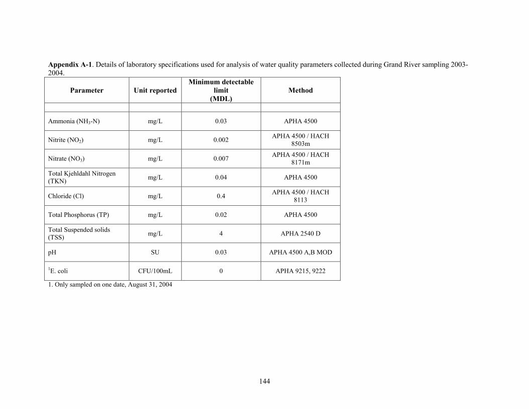
144
Appendix A-1. Details of laboratory specifications used for analysis of water quality parameters collected during Grand River sampling 2003-
2004.
Parameter Unit reported
Minimum detectable
limit
(MDL)
Method
Ammonia (NH3-N) mg/L 0.03 APHA 4500
Nitrite (NO2) mg/L 0.002 APHA 4500 / HACH
8503m
Nitrate (NO3) mg/L 0.007 APHA 4500 / HACH
8171m
Total Kjehldahl Nitrogen
(TKN) mg/L 0.04 APHA 4500
Chloride (Cl) mg/L 0.4 APHA 4500 / HACH
8113
Total Phosphorus (TP) mg/L 0.02 APHA 4500
Total Suspended solids
(TSS) mg/L 4 APHA 2540 D
pH SU 0.03 APHA 4500 A,B MOD
1E. coli CFU/100mL 0 APHA 9215, 9222
1. Only sampled on one date, August 31, 2004

145
Appendix A-2. Objectives and targets proposed by provincial and federal agencies
Parameter Objective Value Agency Purpose
1Ammonia (un-ionized; NH3) 0.02 mg/L
concentration MOE/ PWQO Protection of aquatic life
2Nitrite (NO2) 0.06 mg/L
concentration CCME (federal) / CEQG Protection of aquatic life
3Nitrate nitrogen (NO3-N) <2.93 mg/L
concentration CCME (federal) / CEQG Protection of aquatic life
250 mg/L concentration
Env. Canada Protection of drinking water
Chloride (Cl)
8 mg/L
concentration
Background reference: areas
free from anthropogenic
influence
<0.03 mg/L concentration MOE/ PWQO Eliminate excessive plant
growth in streams and rivers Total Phosphorus (TP)
0.02 mg/L Average concentrations for the
ice free period MOE/ PWQO Avoid nuisance algae in lakes
4Total Suspended solids (TSS)
25 mg/L or 10% of
background
concentration CCME (federal) / CEQG Protection of fish
pH 6.5-8.5 SU concentration
MOE/ PWQO Protection of aquatic life
5E. coli 100 CFU/100mL
concentration MOE
Protection of human health/
beach closings
1. Free (un-ionized) ammonia (dependant on pH and temperature; calculated from formula provided by Emerson et al., 1975)
2. based on RT toxicity tests; many warmwater fish have higher tolerances (e.g. largemouth bass- )
3. protection from direct toxic effects; not related to eutrophication
4. This objective is narrative and has a number of species specific caveats with re: “natural” levels, and duration of exposure (DFO
5. This criteria is based on a specific sampling protocol (geometric mean of 5 samples per site) not followed here. This value is used as a starting point for
general discussion.

146
Appendix A-3. Designation of trophic boundaries based on mean and range concentrations of total nitrogen and total phosphorus.
Trophic State
Parameter (mg/L) Oligotrophic Mesotrophic Eutrophic Hypereutrophic
Total Nitrogen1
< 0.4 mg/L 0.4-0.6 mg/L 0.6-1.5 mg/L > 1.5 mg/L
Total Nitrogen2
Mean 0.661
Range 0.307-1.630 Mean 0.753
Range 0.361-1.387 Mean 1.875
Range 0.393-6.100 -
Total Nitrogen3 < 0.300 0.300 – 0.650 0.650 – 1.500 > 1.500
Total Phosphorus1 < 0.015 mg/L 0.015-0.025 mg/L 0.025-0.1 mg/L > 0.1 mg/L
Total Phosphorus2
Mean 0.008
Range 0.003-0.0177 Mean 0.0267
Range 0.0109-0.0956 Mean 0.0844
Range 0.016-0.386 Range 0.750-1.20
Total Phosphorus3 < 0.009 0.009 – 0.018 0.018 - 0.050 > 0.050
1. LAKEWATCH. 2000. A beginners guide to Water Management – Nutrients IC#102. [http://www.ifas.ufl.edu/~lakewatch/LWcirc.html] 2. Wetzel, R.G. 1983. Limnology. Second Edition. Saunders College Publishing. 860p. 3. Leach, J.H., Johnson, M.G., Kelso, J.R.M. Hartman, J., Mumann, W., and B. Entz. 1977. Responses of percid fishes and their habitats to eutrophication. J.
Fish. Res. Board Can. 34: 1964-1971

147
Appendix B-1. Chlorophyll-a (Chl-a) concentrations from surface waters at seven locations (C1-C7) within the lower reaches of the Grand River,
2003 and 2004. Values are provided for analysis that corrects for the presence of phaeopigments (COR) and that which does not (UC; sometimes
referred to as “total chlorophyll”). Numbers represent the mean of two separate water filtrations and spectrophotometric readings. Date
(dd/MM/YY)
2003 UC COR UC COR UC COR UC COR UC COR UC COR UC COR
23/07/03 50.60 26.80 31.18 19.07 4.21 2.51
06/08/03 26.54 16.77 40.93 29.40 27.93 23.19 6.46 1.74 7.64 3.74 5.63 2.41
13/08/03 41.85 28.20 43.95 30.61 21.53 6.15
25/08/03 61.73 36.95 55.90 30.20 32.18 21.92
02/09/03 43.13 42.92 55.83 28.69 52.66 38.39 14.73 7.15 18.45 9.58 4.52 1.94
09/09/03 64.53 34.35 54.46 40.70 19.58 13.34
15/09/03 19.47 9.49 54.52 19.18 31.16 20.11 24.81 13.16 20.70 12.83 3.90 0.74
23/09/03 23.76 13.83 24.20 16.10 6.41 0.80
29/09/03 17.30 9.02 9.32 6.55 6.85 3.74
07/10/03 31.58 18.78 12.95 4.74 2.93 1.20
16/10/03 36.49 29.00 24.77 16.97 13.55 6.82 8.42 5.35 12.46 8.22 10.90 5.61
21/10/03 7.80 4.28 9.92 4.21 8.02 3.47
27/10/03 11.47 5.88 7.54 4.41 6.91 3.34 5.39 2.74 4.72 2.27 8.14 2.81
2004
15/06/04 40.12 30.27 57.21 46.24 27.22 21.72
23/06/04 24.30 16.97 29.36 22.19 31.14 25.86 36.97 31.07 14.06 11.09
29/06/04 34.74 30.20 41.82 31.47 56.64 45.24 25.40 18.78 11.55 8.22
06/07/04 34.84 23.66 72.73 56.67 42.10 33.61 36.91 29.00 11.50 9.16
13/07/04 60.58 48.51 48.74 39.23 49.16 40.43 33.51 28.47 8.41 6.42
20/07/04 32.10 22.45 31.44 21.18 27.95 19.18 15.42 11.23 8.74 6.55
26/07/04 37.81 28.47 46.06 36.49 33.26 24.46 30.30 22.85 10.95 7.89
03/08/04 37.25 29.34 44.21 37.36 24.02 19.45 23.52 20.18 13.76 11.03
09/08/04 58.25 44.97 61.58 47.58 68.21 53.66 60.68 47.71 25.32 20.31
23/08/04 45.73 32.34 53.62 41.23 41.99 30.07 33.24 26.66 13.96 10.76
30/08/04 30.73 21.45 25.68 16.64 23.47 14.17 22.62 16.57 12.29 8.15
23/09/04 39.39 31.88 75.72 65.22 18.03 14.37 21.96 17.91 14.31 11.43
20/10/04 19.52 14.50 20.42 16.77 13.44 10.22 5.92 4.48 3.43 2.34
(Brantford)
C7
(Betamik harbour)(Port Maitland) (Dun-above dam) (mid Dun- Cayuga) (Cayuga)
C5
(York)
C6C1 C2 C3 C4

148
Appendix C-1A. Benthic invertebrate counts from replicate sampling at 5 stations located in the lower reach of the Grand River, 2002.
GROUP FAMILY TAXON R1 R2 R3 R4 Total R1 R2 R3 R4 Total R1 R2 R3 R4 Total R1 R2 R3 Total
0 0 0 0
OLIGOCHAETA Lumbricidae Lumbricidae incomplete 0 0 1 2 1 4 1 1
Tubificidae Immatures with hair chaetae 0 1 1 2 2 1 5 0
Immatures without hair chaetae 4 11 13 10 38 17 4 21 2 2 2 6 8 15 5 28
Branchiura sowerbyi 1 1 1 2 3 1 6 1 8 2 7 1 10
Limnodrilus cervix 0 1 1 5 3 1 9 1 1 2
Limnodrilus hoffmeisteri 1 3 1 5 0 0 2 2
ACARI Hygrobatidae Hygrobates sp 0 0 0 1 1
Krendowskiidae nr Geayia sp 0 0 0 1 1
Limnesiidae Limnesia sp 1 91 92 0 0 1 1
Unionicolidae Unionicola sp 0 0 1 1 0
COLEOPTERA Elmidae Dubiraphia sp larvae 0 0 1 1 0
DIPTERA Ceratopogonidae Ceratopogonidae type III 1 1 1 1 1 1 1 3 4
Chironomidae 0 0 0 0
Chironominae Chironomus sp 0 18 4 11 1 34 4 7 7 3 21 1 3 4
Cladopelma sp 0 0 1 1 2 0
Cryptochironomus sp 7 8 4 1 20 3 2 1 6 2 2 1 5 2 7 2 11
Dicrotendipes sp 0 0 0 1 1
Glyptotendipes sp gp "A" 1 73 74 0 0 0
Microchironomus sp 1 1 2 2 3 2 2 4 11 1 1
Parachironomus sp 2 2 0 0 0
Polypedilum sg Tripodura sp 63 60 45 1 169 10 3 13 0 3 3
Cladotanytarsus sp 1 1 2 1 1 0 0
Orthocladiinae Orthocladius sp 7 7 0 0 1 1
Tanypodinae Ablabesmyia annulatum gp 0 0 0 1 1 2
Coelotanypus sp 0 1 1 1 1 2 3 2 5
Procladius sp 1 1 2 9 3 12 10 5 17 32 6 7 15 28
Tanypus "concavus" 0 0 1 1 3 1 6 1 1 2
Tanypus neopunctipennis 0 0 1 1 0
Tanypus stellatus 0 0 0 1 1
EPHEMEROPTERA Caenidae Caenis sp 2 1 3 0 0 0
Ephemeridae Hexagenia sp juv 0 1 2 3 0 0
HEMIPTERA Corixidae Palmacorixa nana 0 0 1 1 3 3
GASTROPODA Hydrobiidae Amnicola limosa 0 0 0 1 1
BIVALVIA Sphaeriidae Musculium sp juv 0 0 0 2 2
Musculium transversum 0 0 0 2 2
NEMATODA Unidentified 1 1 1 3 1 1 2 0 0
Total 81 85 66 188 420 63 23 14 1 101 21 35 27 33 116 29 51 37 117
Species Count 9 7 7 10 11 9 3 1 9 14 8 11 12 13 13
Station B5Station B3Station B2Station B1

149
Appendix C-1B. Benthic invertebrate counts from replicate sampling at 5 stations located in the lower reach of the Grand River, 2003
GROUP FAMILY TAXON R1 R2 R3 R4 Total R1 R2 R3 R4 Total R1 R2 R3 R4 Total R1 R2 R3 Total R1 R2 R3 R4 Total
0 0 0 0 0
HIRUDINEA Glossiphoniidae Helobdella stagnalis 0 0 0 0 1 1
OLIGOCHAETA Lumbricidae Sparganophilus sp 0 0 0 2 2 0
Tubificidae Immatures with hair chaetae 2 2 3 3 5 9 7 21 1 1 0
Immatures without hair chaetae 41 35 134 394 604 3 27 78 7 115 87 47 21 2 157 2 5 7 1 1 4 5 11
Branchiura sowerbyi 3 2 5 4 7 11 8 12 7 1 28 1 1 3 1 2 4 10
Limnodrilus cervix 2 1 3 0 5 3 8 0 0
Limnodrilus hoffmeisteri 1 1 7 3 12 0 1 1 0 0
ACARI Limnesiidae Limnesia sp 2 2 0 0 0 0
0 0 0 0 0
COLEOPTERA Elmidae Dubiraphia sp larvae 0 0 1 1 0 1 2 2 1 6
Stenelmis sp larval casts only 0 0 0 0 1 1 2
DIPTERA Ceratopogonidae Ceratopogonidae type III 1 2 7 1 11 3 4 7 1 1 2 1 1 1 1
Chironomidae 0 0 0 0 0
Chironominae Chironomus sp 3 41 12 88 144 9 4 13 4 2 2 8 1 3 4 9 10 2 21
Cryptochironomus sp 11 2 13 2 1 3 0 1 1 1 1
Microchironomus sp 1 1 0 0 1 1 0
Tribelos sp 0 0 0 0 1 1
Cladotanytarsus sp 1 1 0 0 0 0
Tanypodinae Ablabesmyia annulatum gp 5 5 1 1 0 3 3 0
Clinotanypus sp 1 1 3 3 5 6 3 14 8 8 15 8 89 112
Procladius sp 1 2 3 6 6 0 1 1 0
EPHEMEROPTERA Ephemeridae Hexagenia sp juv 0 0 0 2 2 1 1 2 2 6
MEGALOPTERA Sialidae Sialis sp 0 0 0 2 2 1 1
GASTROPODA Viviparidae Campeloma decisum 0 0 0 0 1 1
BIVALVIA Sphaeriidae Musculium sp 0 0 0 4 4 0
Pisidium sp 1 1 0 0 1 1 1 1 2
TURBELLARIA Plagiostomidae Hydrolimax sp 3 1 4 0 0 0 0
NEMATODA Unidentified 1 1 0 0 0 0
Total 64 84 173 492 813 3 47 104 8 162 116 76 43 5 240 26 5 8 39 22 15 29 110 176
Species Count 10 7 9 8 1 6 7 2 8 6 6 3 11 4 2 6 6 7 13
Station B5Station B1 Station B2 Station B3 Station B4

150
Appendix D-1. Metrics used to calculate index of biotic integrity (IBI) values for Grand
River fish communities downstream of Caledonia 2003 and 2004; from Thoma (1999) and
Karr (1981)
# Species – number of native species. List compiled using Cudmore and Crossman (2000)
# Sunfish species – a modification of Karr’s sunfish metric; expanded to include Pomoxis and
Micropterus recognizing that, for Lake Erie watersheds, not all sites have the potential to harbor
all species of sunfish potentially found in the basin.
# Cyprinid species – this metric replaces Karr’s sucker species metric; which can be naturallry
low in abundance and numbers in L. Erie drowned river mouth systems. Whereas cyprinid
species were traditionally a prominent component of these systems.
# Benthic species – modification of Karr’s darter metric. It provides a good range and
environmental responsiveness within L. Erie and lower watersheds. It responds primarily to
environmental disturbance from sedimentation and low oxygen levels. List attempts to maintain
Karr’s original sensitivity and so tolerant benthic species such as bullheads and suckers were
excluded.
% Phytophillic individuals – modified from Karr’s % insectivorous cyprinids.
% Top carnivores - follows metric from Karr
# Intolerant species – variation from Karr; utilizes Ohio EPA listings (Ohio EPA 1988).
Includes: mooneye, black redhorse, greater redhorse, river redhorse, redside dace, hornyhead
chub, river chub, pugnose shiner, blackchin shiner, blacknose shiner, rosyface shiner, mimic
shiner, pugnose minnow, longnose dace, silver shiner, stonecat, brindled madtom, northern
madtom, eastern sand darter, channel darter
% Omnivore individuals - follows metric from Karr; included gizzard shad
% Nonindigenous individuals – utilizes Cudmore and Crossman (2000)
% Tolerant individuals - utilizes Ohio EPA listings (Ohio EPA 1988). Includes:
central mudminnow, white sucker, goldfish, carp, golden shiner, bluntnose minnow, fathead
minnow, blacknose dace, creek chub, yellow bullhead, brown bullhead, banded killifish, green
sunfish, goldfish x carp, Ictaluridae hybrids: black x brown bullhead, yellow x brown bullhead,
mirror carp
% DELT (observable deformities, eroded fins, lesions, tumours) follows Ohio EPA methods for
classifiying external deformities; note: not used in this case because of concern over inconsistent
record keeping.
Relative numbers – standardized by fishing time (electroseconds)

151
Appendix E-1. Dunnville Marsh Water Temperatures Summer, 2002
A temperature logger (Optic StowAway Temp; Onset Computer Corp, MA) set to record hourly
temperatures was deployed in the Dunnville Marshes, downstream of Dunnville ON, in
association with the Maple Ck. drainage, from July 9 to August 31, 2002. Mean, minimum and
maximum daily temperatures are displayed relative to walleye thermal reference points from
Hokanson (1977).
k
Logger location
01/Jul 15/Jul 29/Jul 12/Aug 26/Aug
Te
mpe
ratu
re (
oC
)
10
15
20
25
30
35
40
Minimum Daily Temperature
Mean Daily Temperature
Maximum Daily Temperature
Walleye Upper Incipient Lethal
YOY walleye (< 6.5cm TL) optima
Adult walleye physiological optima

152
APPENDIX E-2A. Locations of sampling sites where water column temperature and
oxygen profiles were collected in August and September, 2002.
9
8
7
6
5
4321
1615
14
13
12
11
10
26 25 24
23
22
2120
19
18
17
Southern Grand River Watershed; Brantford to Port Maitland/Lake Erie

153
Appendix E-2B. Description of 2002 water column temperature and oxygen profile sample site locations.
2002 Temp/DO
Profile StationsDescription
Regular site in 2003 -
2005 profiling
Stn ID 14-Aug-02 09-Sep-02 10-Sep-02 Latitude Longitude
1 + Sulphur Ck Weir 4 42.899 -79.640
2 + Sulphur Ck Channel 3-4 42.897 -79.638
3 + + Sulphur Ck. Campsites 42.896 -79.635
4 + + Sulphur Ck. Fishway 42.896 -79.629
5 + Sulphur Ck. Weir 2 42.895 -79.624
6 + + Dunnville dam plungepool 42.900 -79.619
7 + Main (near sunfish ck mouth) 42.897 -79.610
8 + + Main channel near Betamik harbour 42.895 -79.599 TO-3
9 + Main channel btwn Betamik & P_shipyard 42.888 -79.593
10 + + Main channel near maple ck. 42.883 -79.574 TO-2
11 + Main channel near maple ck. "outlet" 42.877 -79.567
12 + Main channel near Broad ck 42.872 -79.570
13 + + Main channel near shipyard 42.862 -79.575 TO-1 (close)
14 + Main channel btwn piers 42.857 -79.577
15 + Lake directly out from west pier 42.852 -79.579
16 + Lake nearshore in plume 42.852 -79.576
17 + Main directly above dam 42.901 -79.621 TO-4
18 + Byng park upstream boat launch 42.905 -79.651
19 + Main channel- Evergreen Point 42.913 -79.654 TO-5
20 + Upstream end of first embayment 42.919 -79.663
21 + Private camp shoreline 42.921 -79.678 TO-6 (close)
22 + Fish Community station #63 42.932 -79.689
23 + just downstream of private RV resort 42.923 -79.717 TO-7
24 + private RV resort 42.918 -79.735
25 + Main channel near power lines 42.918 -79.762 TO-8
26 + Fish Community station #64 42.917 -79.788
Sample Dates Co-ordinates

154
Appendix E-2C. Summary of temperature and oxygen profile data, Grand River, August and September, 2002
Station ID / Date
Max ∆D Max Min ∆T Max Min ∆ % Max Min ∆DO
Aug/14
3 1.0 0.5 27.2 26.3 -0.9 76.8 58.5 -18.3 6.1 4.7 -1.4
4 1.4 0.5 27.3 26.7 -0.6 92.8 83.4 -9.4 7.4 6.8 -0.6
6 8.0 7.2 27.1 26.1 -1.0 102.1 80.5 -21.6 8.1 6.5 -1.6
8 2.5 1.9 27.6 26.6 -0.9 110.1 74.3 -35.8 8.7 6.0 -2.7
10 4.0 3.5 28.3 26.5 -1.8 114.3 69.7 -44.6 8.9 5.6 -3.3
13 5.1 4.1 27.9 26.4 -1.5 103.1 52.2 -50.9 8.1 4.2 -3.9
Sep/09
1 2.4 1.9 24.5 23.7 -0.8 91.8 74.9 -16.9 7.7 6.4 -1.3
2 1.4 0.9 23.8 23.5 -0.3 86.2 78.8 -7.4 7.3 6.7 -0.6
3 1.0 0.4 23.7 23.5 -0.2 84.3 68.8 -15.5 7.2 5.9 -1.3
4 2.1 1.6 24.1 23.9 -0.2 91.5 87.3 -4.2 7.8 7.4 -0.4
5 1.7 1.2 24.4 23.5 -0.9 88.5 71.8 -16.7 7.4 6.1 -1.3
6 9.8 9.3 24.8 24.1 -0.7 99.6 82.7 -16.9 8.3 7.0 -1.3
7 3.0 2.4 27.1 24.1 -3.0 125.9 77.5 -48.4 10.1 6.6 -3.5
8 2.6 2.1 27.1 24.2 -2.9 128.1 44.3 -83.8 10.3 3.7 -6.5
9 3.3 2.8 26.9 24.4 -2.5 124.2 64.8 -59.4 10.0 5.4 -4.5
10 4.0 3.5 26.8 23.8 -3.0 116.8 36.2 -80.6 9.4 3.1 -6.3
11 3.4 2.9 26.0 24.4 -1.5 109.8 63.3 -46.5 9.0 5.3 -3.7
12 2.9 2.4 26.1 24.3 -1.8 117.1 63.4 -53.7 9.5 5.3 -4.2
13 4.3 3.8 25.6 23.5 -2.0 112.0 32.5 -79.5 9.2 2.8 -6.5
14 6.6 6.0 24.9 23.7 -1.2 103.8 42.0 -61.8 8.7 3.6 -5.1
15 7.1 6.6 24.8 23.4 -1.4 105.6 48.6 -57.0 8.9 4.1 -4.7
16 3.9 3.4 24.7 23.2 -1.5 104.3 27.8 -76.5 8.7 2.4 -6.4
17 2.0 1.5 24.4 24.0 -0.4 91.5 63.9 -27.6 7.7 5.4 -2.3
18 1.7 1.6 24.9 23.6 -1.3 103.2 28.5 -74.7 8.6 2.4 -6.2
19 2.9 2.3 25.3 23.5 -1.8 125.2 41.8 -83.4 10.3 3.6 -6.8
20 3.1 2.6 25.2 23.5 -1.8 127.3 46.5 -80.8 10.5 4.0 -6.6
21 2.5 1.9 24.6 23.6 -1.0 127.6 65.5 -62.1 10.7 5.6 -5.1
22 2.9 2.4 25.0 23.4 -1.6 127.8 45.9 -81.9 10.6 3.9 -6.7
23 2.9 2.4 25.3 23.1 -2.2 139.9 38.6 -101.3 11.6 3.3 -8.3
24 4.0 3.5 24.8 22.7 -2.0 137.6 8.0 -129.6 11.5 0.7 -10.8
25 2.3 2.1 24.3 23.5 -0.8 115.0 80.8 -34.2 9.7 6.9 -2.8
26 3.5 3.5 25.0 22.3 -2.7 118.8 7.2 -111.6 9.9 0.6 -9.2
Depth
DO - % Saturation DO (mg/L)
Dissolved OxygenTemperature
(oC)

155
Appendix E-2D. Water column profiles of temperature and oxygen, Grand River, August
and September, 2002.
August 14, 2002
Depth (m)
0 2 4 6 8 10
Dis
so
lve
d O
xyg
en
(m
g /
L)
3
4
5
6
7
8
9
10
Stn 3
Stn 4
Stn 6
Stn 8
Stn 10
Stn 13
August 14, 2002
Depth (m)
0 2 4 6 8 10
Tem
pe
ratu
re (
oC
)
25.5
26.0
26.5
27.0
27.5
28.0
28.5
Stn 3
Stn 4
Stn 6
Stn 8
Stn 10
Stn 13

Appendix E-2D cont’d
Temperature (oC)Dissolved Oxygen (mg/L)
156
Stn. 1. September 9, 2002
Depth (m)
0 2 4 6 8 10
Dis
so
lve
d O
xyg
en
(m
g/L
)
0
5
10
15
20
Te
mp
era
ture
(oC
)
15
20
25
30
35
Stn. 3. September 9, 2002
Depth (m)
0 2 4 6 8 10
Dis
so
lve
d O
xyg
en
(m
g/L
)
0
5
10
15
20
Te
mp
era
ture
(oC
)
15
20
25
30
35
Stn. 5. September 9, 2002
Depth (m)
0 2 4 6 8 10
Dis
so
lve
d O
xyg
en
(m
g/L
)
0
5
10
15
20
Te
mp
era
ture
(oC
)
15
20
25
30
35
Stn. 7. September 9, 2002
Depth (m)
0 2 4 6 8 10
Dis
so
lve
d O
xyg
en
(m
g/L
)
0
5
10
15
20
Te
mp
era
ture
(oC
)
15
20
25
30
35
Stn. 2. September 9, 2002
Depth (m)
0 2 4 6 8 10
Dis
so
lve
d O
xyg
en
(m
g/L
)
0
5
10
15
20
Te
mp
era
ture
(oC
)
15
20
25
30
35
Stn. 4. September 9, 2002
Depth (m)
0 2 4 6 8 10
Dis
so
lve
d O
xyg
en
(m
g/L
)
0
5
10
15
20
Te
mp
era
ture
(oC
)
15
20
25
30
35
Stn. 6. September 9, 2002
Depth (m)
0 2 4 6 8 10
Dis
so
lve
d O
xyg
en
(m
g/L
)
0
5
10
15
20
Te
mp
era
ture
(oC
)
15
20
25
30
35
Stn. 8. September 9, 2002
Depth (m)
0 2 4 6 8 10
Dis
so
lve
d O
xyg
en
(m
g/L
)
0
5
10
15
20
Te
mp
era
ture
(oC
)
15
20
25
30
35

Appendix E-2D cont’d
Temperature (oC)Dissolved Oxygen (mg/L)
157
Stn. 1. September 9, 2002
Depth (m)
0 2 4 6 8 10
Dis
so
lve
d O
xyg
en
(m
g/L
)
0
5
10
15
20
Te
mp
era
ture
(oC
)
15
20
25
30
35
Stn. 3. September 9, 2002
Depth (m)
0 2 4 6 8 10
Dis
so
lve
d O
xyg
en
(m
g/L
)
0
5
10
15
20
Te
mp
era
ture
(oC
)
15
20
25
30
35
Stn. 5. September 9, 2002
Depth (m)
0 2 4 6 8 10
Dis
so
lve
d O
xyg
en
(m
g/L
)
0
5
10
15
20
Te
mp
era
ture
(oC
)
15
20
25
30
35
Stn. 7. September 9, 2002
Depth (m)
0 2 4 6 8 10
Dis
so
lve
d O
xyg
en
(m
g/L
)
0
5
10
15
20
Te
mp
era
ture
(oC
)
15
20
25
30
35
Stn. 2. September 9, 2002
Depth (m)
0 2 4 6 8 10
Dis
so
lve
d O
xyg
en
(m
g/L
)
0
5
10
15
20
Te
mp
era
ture
(oC
)
15
20
25
30
35
Stn. 4. September 9, 2002
Depth (m)
0 2 4 6 8 10
Dis
so
lve
d O
xyg
en
(m
g/L
)
0
5
10
15
20
Te
mp
era
ture
(oC
)
15
20
25
30
35
Stn. 6. September 9, 2002
Depth (m)
0 2 4 6 8 10
Dis
so
lve
d O
xyg
en
(m
g/L
)
0
5
10
15
20
Te
mp
era
ture
(oC
)
15
20
25
30
35
Stn. 8. September 9, 2002
Depth (m)
0 2 4 6 8 10
Dis
so
lve
d O
xyg
en
(m
g/L
)
0
5
10
15
20
Te
mp
era
ture
(oC
)
15
20
25
30
35

Appendix E-2D cont’d
Temperature (oC)Dissolved Oxygen (mg/L)
158
Stn. 9. September 9, 2002
Depth (m)
0 2 4 6 8 10
Dis
so
lve
d O
xyg
en
(m
g/L
)
0
5
10
15
20
Te
mp
era
ture
(oC
)
15
20
25
30
35
Stn. 11. September 9, 2002
Depth (m)
0 2 4 6 8 10
Dis
so
lve
d O
xyg
en
(m
g/L
)
0
5
10
15
20
Te
mp
era
ture
(oC
)
15
20
25
30
35
Stn. 13. September 9, 2002
Depth (m)
0 2 4 6 8 10
Dis
so
lve
d O
xyg
en
(m
g/L
)
0
5
10
15
20
Te
mp
era
ture
(oC
)
15
20
25
30
35
Stn. 15. September 9, 2002
Depth (m)
0 2 4 6 8 10
Dis
so
lve
d O
xyg
en
(m
g/L
)
0
5
10
15
20
Te
mp
era
ture
(oC
)
15
20
25
30
35
Stn. 10. September 9, 2002
Depth (m)
0 2 4 6 8 10
Dis
so
lve
d O
xyg
en
(m
g/L
)
0
5
10
15
20
Te
mp
era
ture
(oC
)
15
20
25
30
35
Stn. 12. September 9, 2002
Depth (m)
0 2 4 6 8 10
Dis
so
lve
d O
xyg
en
(m
g/L
)
0
5
10
15
20
Te
mp
era
ture
(oC
)
15
20
25
30
35
Stn. 14. September 9, 2002
Depth (m)
0 2 4 6 8 10
Dis
so
lve
d O
xyg
en
(m
g/L
)
0
5
10
15
20
Te
mp
era
ture
(oC
)
15
20
25
30
35
Stn. 16. September 9, 2002
Depth (m)
0 2 4 6 8 10
Dis
so
lve
d O
xyg
en
(m
g/L
)
0
5
10
15
20
Te
mp
era
ture
(oC
)
15
20
25
30
35

Appendix E-2D cont’d
Temperature (oC)Dissolved Oxygen (mg/L)
159
Stn. 17., September 10, 2002
Depth (m)
0 1 2 3 4
Dis
so
lve
d O
xyg
en
(m
g/L
)
0
5
10
15
20
Te
mp
era
ture
(oC
)
15
20
25
30
35
Stn. 19. September 10, 2002
Depth (m)
0 1 2 3 4
Dis
so
lve
d O
xyg
en
(m
g/L
)
0
5
10
15
20
Te
mp
era
ture
(oC
)
15
20
25
30
35
Stn. 21. September 10, 2002
Depth (m)
0 1 2 3 4
Dis
so
lve
d O
xyg
en
(m
g/L
)
0
5
10
15
20
Te
mp
era
ture
(oC
)
15
20
25
30
35
Stn. 23. September 10, 2002
Depth (m)
0 1 2 3 4
Dis
so
lve
d O
xyg
en
(m
g/L
)
0
5
10
15
20
Te
mp
era
ture
(oC
)
15
20
25
30
35
Stn. 18. September 10, 2002
Depth (m)
0 1 2 3 4
Dis
so
lve
d O
xyg
en
(m
g/L
)
0
5
10
15
20
Te
mp
era
ture
(oC
)
15
20
25
30
35
Stn. 20. September 10, 2002
Depth (m)
0 1 2 3 4
Dis
so
lve
d O
xyg
en
(m
g/L
)
0
5
10
15
20
Te
mp
era
ture
(oC
)
15
20
25
30
35
Stn. 22. September 10, 2002
Depth (m)
0 1 2 3 4
Dis
so
lve
d O
xyg
en
(m
g/L
)
0
5
10
15
20
Te
mp
era
ture
(oC
)
15
20
25
30
35
Stn. 24. September 10, 2002
Depth (m)
0 1 2 3 4
Dis
so
lve
d O
xyg
en
(m
g/L
)
0
5
10
15
20
Te
mp
era
ture
(oC
)
15
20
25
30
35

Appendix E-2D cont’d
Temperature (oC)Dissolved Oxygen (mg/L)
160
Stn. 25. September 10, 2002
Depth (m)
0 1 2 3 4
Dis
so
lve
d O
xyg
en
(m
g/L
)
0
5
10
15
20
Te
mp
era
ture
(oC
)
15
20
25
30
35
Stn. 26. September 10, 2002
Depth (m)
0 1 2 3 4
Dis
so
lve
d O
xyg
en
(m
g/L
)
0
5
10
15
20
Te
mp
era
ture
(oC
)
15
20
25
30
35

161
Appendix E-3. Temperature and oxygen: continuous logging at depth. Picture of bracket
for holding and protecting logging equipment.
0.5 m above
substrate

Appendix E-4. Descriptive Statistics of temperatures collected at logging stations (TL1-
TL10) within the southern Grand River, 2001-2005.
162
TL1 Minimum Mean Maximum St. Dev.
April 5.42 9.51 14.27 2.43
May 6.51 11.58 18.73 3.90
June 10.54 15.93 22.01 2.08
July 12.56 20.25 25.61 2.85
August 17.60 23.21 25.61 1.31
September 14.58 20.16 23.87 2.56
October 7.44 12.60 17.44 2.71
November 6.20 8.12 9.92 0.94
December 0.04 3.91 7.60 2.35
January 0.04 0.31 1.48 0.32
February -0.11 0.86 3.07 0.84
March 0.04 2.74 6.20 1.62
April 3.23 9.74 17.76 3.97
May 8.83 12.64 20.52 2.22
June 10.08 19.16 25.44 2.69
July 19.39 23.49 28.10 1.57
August 23.02 25.56 28.47 1.32
September 18.24 22.37 25.61 1.84
October 7.13 13.96 20.68 3.97
November 1.80 5.55 9.30 1.88
December -0.11 0.48 1.64 0.36
January -0.11 0.17 0.52 0.11
February 0.04 0.15 0.68 0.14
March -0.11 1.18 6.82 2.12
April 0.52 7.64 15.06 4.32
May 12.09 14.98 19.06 1.64
June 15.22 20.26 25.44 2.60
July 21.01 23.81 26.67 1.05
August 23.19 25.26 27.56 0.90
September 14.58 20.49 23.53 2.18
October 8.22 12.00 16.01 1.92
November 3.23 6.51 10.54 2.04
December -0.11 1.08 3.70 0.86
January -0.28 0.49 3.70 1.09
February] -0.11 0.07 0.36 0.09
March -0.11 2.18 8.99 2.41
April 4.01 9.41 14.42 3.06
May 11.01 16.51 21.68 3.10
June 16.96 20.75 24.04 1.52
July 21.51 23.46 25.61 0.96
August 21.01 22.71 25.78 0.91
September 18.73 21.55 25.26 1.57
October 9.30 13.35 19.87 2.87
November 4.32 7.00 11.47 1.86
December -0.11 1.52 7.29 1.70
January -0.11 0.31 2.59 0.53
February 0.04 0.10 0.20 0.08
March 0.04 0.52 4.32 1.08
April 2.28 8.35 12.72 2.83
May 8.83 12.98 16.33 2.65
June 20.68 24.65 28.10 2.12
July 23.87 26.54 29.94 1.27
August 22.34 25.36 28.28 1.57
September 21.84 22.82 23.70 0.43
2005
2001
2002
2003
2004

Appendix E-4. Descriptive Statistics of temperatures collected at logging stations (TL1-
TL10) within the southern Grand River, 2001-2005.
163
TL2 Minimum Mean Maximum St. Dev.
April 5.27 9.96 17.27 2.94
May 14.11 17.92 20.67 1.30
June 14.89 21.78 27.70 3.76
July 20.99 24.22 28.24 1.81
August 22.33 25.39 28.79 1.69
September 14.73 20.30 25.06 2.71
October 7.14 12.59 18.07 2.75
November 5.58 8.11 10.39 0.99
December 0.05 3.82 7.76 2.37
January -0.10 0.28 1.81 0.36
February -0.10 0.89 3.39 0.89
March -0.10 2.80 6.67 1.69
April 2.92 9.81 18.56 4.06
May 8.84 13.15 21.33 2.83
June 18.07 22.27 27.70 2.26
July 24.02 26.34 29.53 1.02
August 22.33 25.51 28.98 1.43
September 18.07 22.37 25.93 1.88
October 6.21 13.35 20.83 4.27
November 1.18 5.38 9.77 2.04
December -0.10 0.50 1.97 0.37
January 0.05 0.18 0.37 0.12
February 0.05 0.09 0.37 0.07
March -0.10 1.17 7.14 2.19
April 0.37 7.82 15.53 4.45
May 12.09 15.00 19.69 1.70
June 15.68 20.57 26.46 2.81
July 21.33 24.16 27.52 1.38
August 22.83 25.18 27.52 0.93
September 14.26 20.36 23.51 2.21
October 7.61 11.45 15.21 1.89
November 3.24 6.52 10.39 2.03
December -0.10 1.14 3.71 0.88
January -0.10 0.49 3.71 1.13
February -0.10 0.03 0.21 0.06
March -0.10 2.32 8.38 2.41
April 4.18 9.69 14.57 3.06
May 10.55 16.65 22.33 3.08
June 16.32 20.87 24.37 1.67
July 21.33 23.48 26.11 1.04
August 20.99 22.80 26.46 0.99
September 18.39 21.39 25.06 1.61
October 9.46 13.14 19.37 2.81
November 4.18 6.98 11.32 1.85
December -0.10 1.48 5.12 1.61
January -0.10 0.23 3.39 0.66
February -0.10 -0.04 0.21 0.07
March -0.10 0.53 5.12 1.35
April 1.81 8.91 14.73 3.13
May 8.53 14.85 20.50 3.10
June 19.04 24.33 28.79 2.45
July 24.37 26.79 29.72 1.21
August 22.33 25.30 28.06 1.66
September 21.66 22.84 24.19 0.66
2005
2001
2002
2003
2004

Appendix E-4. Descriptive Statistics of temperatures collected at logging stations (TL1-
TL10) within the southern Grand River, 2001-2005.
164
TL3 Minimum Mean Maximum St. Dev.
April -0.59 6.94 15.51 4.42
May 11.14 14.14 18.05 1.60
June 13.93 19.59 26.26 2.89
July 21.80 24.53 26.78 1.18
March -0.08 2.46 8.39 2.43
April 3.73 9.59 15.22 3.09
May 10.40 16.56 22.49 3.12
June 16.17 20.72 24.88 1.72
July 20.67 23.44 26.45 1.23
August 20.02 22.70 26.10 1.19
September 17.59 21.31 25.92 1.93
October 8.85 12.97 20.18 2.73
November 4.04 6.78 11.95 1.95
December -0.24 1.30 4.98 1.59
January -0.24 -0.01 2.63 0.54
February -0.24 -0.22 0.08 0.05
March -0.24 0.17 4.19 0.97
April 1.52 8.65 15.85 3.05
May 7.93 14.40 20.67 2.99
June 17.59 23.95 29.52 2.62
July 22.49 26.30 30.83 1.63
August 20.99 24.77 28.61 1.90
September 19.86 22.33 24.54 1.19
2003
2004
2005
TL4 Minimum Mean Maximum St. Dev.
April 7.75 7.75 16.71 4.44
May 14.92 14.92 19.62 1.80
June 20.48 20.48 28.17 3.09
July 25.66 25.66 29.09 1.43
March 2.52 2.52 9.93 2.55
April 9.57 9.57 15.53 3.19
May 16.58 16.58 22.82 3.24
March 3.00 3.00 3.72 0.39
April 8.75 8.75 16.47 3.12
May 14.63 14.63 20.83 3.15
2003
2004
2005

Appendix E-4. Descriptive Statistics of temperatures collected at logging stations (TL1-
TL10) within the southern Grand River, 2001-2005.
165
TL5 Minimum Mean Maximum St. Dev.
July 24.04 26.62 29.74 1.01
August 22.68 25.98 30.68 1.55
September 17.92 22.83 27.90 2.12
October 6.22 13.51 21.67 4.28
November 0.56 5.35 10.72 2.18
December -0.08 0.46 1.03 0.28
January -0.08 0.26 0.88 0.31
February -0.08 0.12 0.56 0.18
March -0.08 1.20 7.31 2.16
April -0.08 8.02 17.12 4.48
May 11.79 14.97 19.22 1.72
June 15.38 21.02 27.90 3.20
July 21.84 24.78 29.00 1.62
August 23.01 25.58 28.63 1.05
September 14.27 20.60 24.91 2.43
October 7.00 11.37 16.17 2.06
November 3.10 6.39 10.72 2.08
December -0.24 1.10 3.57 0.87
January -0.24 0.54 4.19 1.09
February -0.08 0.09 0.56 0.17
March -0.08 2.30 7.93 2.39
April 4.04 9.62 14.90 3.10
May 9.94 16.59 22.84 3.14
June 16.48 21.02 25.77 1.90
July 21.51 23.84 27.36 1.25
August 21.01 23.13 27.18 1.16
September 18.73 21.83 27.01 1.73
October 9.01 13.17 20.35 3.01
November 3.10 6.81 11.64 1.92
December -0.24 1.48 5.13 1.53
January -0.24 0.13 3.26 0.62
February -0.24 -0.07 0.07 0.07
March -0.08 0.51 4.66 1.21
April 1.36 8.89 17.28 3.29
May 8.23 15.10 21.67 3.39
June 18.89 25.12 31.44 2.82
July 24.38 27.31 33.19 1.59
August 22.01 25.69 29.93 1.94
September 21.67 23.24 25.60 0.98
2002
2003
2004
2005
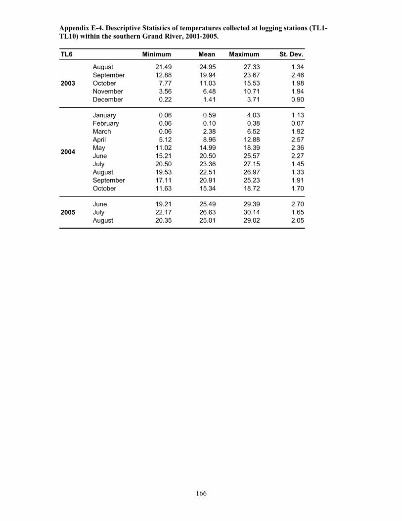
Appendix E-4. Descriptive Statistics of temperatures collected at logging stations (TL1-
TL10) within the southern Grand River, 2001-2005.
166
TL6 Minimum Mean Maximum St. Dev.
August 21.49 24.95 27.33 1.34
September 12.88 19.94 23.67 2.46
October 7.77 11.03 15.53 1.98
November 3.56 6.48 10.71 1.94
December 0.22 1.41 3.71 0.90
January 0.06 0.59 4.03 1.13
February 0.06 0.10 0.38 0.07
March 0.06 2.38 6.52 1.92
April 5.12 8.96 12.88 2.57
May 11.02 14.99 18.39 2.36
June 15.21 20.50 25.57 2.27
July 20.50 23.36 27.15 1.45
August 19.53 22.51 26.97 1.33
September 17.11 20.91 25.23 1.91
October 11.63 15.34 18.72 1.70
June 19.21 25.49 29.39 2.70
July 22.17 26.63 30.14 1.65
August 20.35 25.01 29.02 2.05
2003
2004
2005
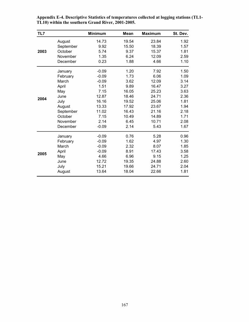
Appendix E-4. Descriptive Statistics of temperatures collected at logging stations (TL1-
TL10) within the southern Grand River, 2001-2005.
167
TL7 Minimum Mean Maximum St. Dev.
August 14.73 19.54 23.84 1.92
September 9.92 15.50 18.39 1.57
October 5.74 9.37 15.37 1.81
November 1.35 6.24 12.09 2.59
December 0.23 1.88 4.66 1.10
January -0.09 1.20 7.92 1.50
February -0.09 1.73 6.06 1.09
March -0.09 3.62 12.09 3.14
April 1.51 9.89 16.47 3.27
May 7.15 16.05 25.23 3.63
June 12.87 18.46 24.71 2.36
July 16.16 19.52 25.06 1.81
August 13.33 17.92 23.67 1.94
September 11.02 16.43 21.16 2.18
October 7.15 10.49 14.89 1.71
November 2.14 6.45 10.71 2.08
December -0.09 2.14 5.43 1.67
January -0.09 0.76 5.28 0.96
February -0.09 1.62 4.97 1.30
March -0.09 2.32 8.07 1.85
April -0.09 8.91 17.43 3.58
May 4.66 6.96 9.15 1.25
June 12.72 19.35 24.88 2.60
July 15.21 19.66 24.71 2.04
August 13.64 18.04 22.66 1.81
2003
2004
2005

Appendix E-4. Descriptive Statistics of temperatures collected at logging stations (TL1-
TL10) within the southern Grand River, 2001-2005.
168
TL8 Minimum Mean Maximum St. Dev.
August 19.83 24.02 27.31 1.59
September 12.54 19.10 23.82 2.58
October 7.13 10.21 16.13 2.11
November 2.60 5.52 9.91 1.92
December -0.92 0.49 2.76 0.97
January -0.75 -0.25 3.38 1.11
February -0.75 -0.75 -0.75 0.00
March -0.92 1.56 7.13 2.24
April 3.86 8.79 14.71 3.09
May 9.29 15.24 20.97 2.97
October 9.62 11.22 13.18 0.77
November 3.58 6.55 11.79 1.95
December -0.24 1.18 4.82 1.60
January -0.24 0.20 3.11 0.69
February -0.24 -0.13 0.72 0.13
March -0.24 1.06 4.67 1.55
April 1.36 8.53 16.48 3.24
May 8.08 14.55 20.99 3.38
June 18.56 24.48 31.22 3.15
July 21.82 26.37 31.99 2.11
August 20.02 24.76 30.27 2.42
2003
2004
2005

Appendix E-4. Descriptive Statistics of temperatures collected at logging stations (TL1-
TL10) within the southern Grand River, 2001-2005.
169
TL9 Minimum Mean Maximum St. Dev.
August 18.57 23.87 28.80 2.13
September 11.49 18.99 25.42 3.09
October 6.38 10.02 17.77 2.19
November 2.14 6.21 11.81 2.38
December -0.08 0.97 3.42 0.94
January 0.07 0.62 5.76 1.30
February 0.07 0.07 0.23 0.01
March 0.07 2.77 10.26 3.01
April 4.19 10.10 16.02 3.07
May 8.39 16.57 23.86 3.40
June 14.43 20.62 28.07 2.68
July 18.90 22.84 29.35 2.35
August 16.49 21.85 28.43 2.32
September 13.35 20.02 27.35 2.91
October 7.16 11.86 19.38 2.62
November 1.19 6.12 12.42 2.26
December 0.07 1.36 4.82 1.54
January 0.07 0.30 3.26 0.41
February 0.07 0.11 0.23 0.07
March 0.07 0.37 4.35 0.71
April 0.07 9.16 17.77 3.63
May 7.78 15.19 23.52 3.53
June 17.12 24.74 32.19 3.71
July 19.87 26.27 33.96 2.68
August 17.77 23.99 31.03 2.81
2003
2004
2005

Appendix E-4. Descriptive Statistics of temperatures collected at logging stations (TL1-
TL10) within the southern Grand River, 2001-2005.
170
TL10 Minimum Mean Maximum St. Dev.
August 20.43 24.56 28.36 1.58
September 13.25 19.87 26.03 2.78
October 7.98 10.91 17.67 2.07
November 3.14 6.33 10.62 1.96
December -0.04 1.28 3.46 0.95
January -0.04 0.49 4.39 1.18
February -0.04 0.02 0.59 0.12
March -0.04 2.48 8.13 2.33
April 4.71 9.61 15.12 3.01
May 10.15 15.78 21.41 2.92
June 14.97 20.04 25.16 1.98
July 19.62 22.77 26.74 1.45
August 18.64 22.12 26.21 1.51
September 16.71 20.66 26.03 2.10
October 8.13 12.61 21.41 2.77
November 3.93 6.79 12.16 1.92
December -0.21 1.38 5.02 1.57
January -0.04 0.60 2.83 0.57
February -0.04 0.18 1.24 0.19
March -0.04 1.09 4.55 1.26
April 1.24 8.53 16.08 3.20
May 8.29 14.32 20.43 3.18
June 18.31 24.21 31.53 3.10
July 21.91 26.25 32.12 2.08
August 20.11 24.68 30.96 2.41
2003
2004
2005

Appendix E-5. Distribution of hourly temperatures measured between November 26, 2004
and September 1, 2006 at 11 stations in the Grand River
171
TL1
Temperature Range (oC)
-5 0 5 10 15 20 25 30 35
Coun
t
0
100
200
300
400
5001171
TL2
Temperature range (oC)
-5 0 5 10 15 20 25 30 35
Coun
t
0
100
200
300
400
500547 646
TL5
Temperature range (oC)
-5 0 5 10 15 20 25 30 35
Coun
t
0
100
200
300
400
500
600
741
TL7
Temperature range (oC)
-5 0 5 10 15 20 25 30 35
Coun
t
0
100
200
300
400
500
TL8
Temperature range (oC)
-5 0 5 10 15 20 25 30 35
Coun
t
0
100
200
300
400
500906
TL9
Temperature range (oC)
-5 0 5 10 15 20 25 30 35
Coun
t
0
100
200
300
400
5001252
TL10
Temperature range (oC)
-5 0 5 10 15 20 25 30 35
Coun
t
0
100
200
300
400
500723
TQ4
Temperature range (oC)
-5 0 5 10 15 20 25 30 35
Coun
t
0
100
200
300
400
500979
953
577

Appendix E-5. Distribution of hourly temperatures measured between November 26, 2004
and September 1, 2006 at 11 stations in the Grand River
172
TQ3
Temperature range (oC)
-5 0 5 10 15 20 25 30 35
Cou
nt
0
100
200
300
400
500868 TQ2
Temperature range (oC)
-5 0 5 10 15 20 25 30 35
Coun
t
0
100
200
300
400
500600 526
TQ1
Temperature range (oC)
-5 0 5 10 15 20 25 30 35
Coun
t
0
100
200
300
400
500

Appendix E6: Temperature and oxygen profiles, Grand River, 2004.
Temperature (oC)Dissolved Oxygen (mg/L)
173
Stn. 5., 3:00 pm, June 15, 2004
Depth (m)
0 1 2 3 4 5 6
Dis
so
lve
d O
xyge
n (
mg/L
)
0
5
10
15
20
Te
mp
era
ture
(oC
)
15
20
25
30
35
Stn. 7., 4:00 pm, June 15, 2004
Depth (m)
0 1 2 3 4 5 6
Dis
so
lve
d O
xyge
n (
mg/L
)
0
5
10
15
20
Te
mp
era
ture
(oC
)
15
20
25
30
35
Stn. 9., 5:00 pm, June 15, 2004
Depth (m)
0 1 2 3 4 5 6
Dis
so
lve
d O
xyge
n (
mg/L
)
0
5
10
15
20
Te
mp
era
ture
(oC
)
15
20
25
30
35
Stn. 6., 3:30 pm, June 15, 2004
Depth (m)
0 1 2 3 4 5 6
Dis
so
lve
d O
xyge
n (
mg/L
)
0
5
10
15
20
Te
mp
era
ture
(oC
)
15
20
25
30
35
Stn. 8., 4:40 pm, June 15, 2004
Depth (m)
0 1 2 3 4 5 6
Dis
so
lve
d O
xyge
n (
mg/L
)
0
5
10
15
20
Te
mp
era
ture
(oC
)
15
20
25
30
35
Stn. 10., 5:20 pm, June 15, 2004
Depth (m)
0 1 2 3 4 5 6
Dis
so
lve
d O
xyge
n (
mg/L
)
0
5
10
15
20
Te
mp
era
ture
(oC
)
15
20
25
30
35
Stn. 1., 11:55 am, June 23, 2004
Depth (m)
0 1 2 3 4 5 6 7
Dis
so
lve
d O
xyge
n (
mg/L
)
0
5
10
15
20
Te
mp
era
ture
(oC
)
15
20
25
30
35
Stn. 2., 12:20 pm, June 23, 2004
Depth (m)
0 1 2 3 4 5 6 7
Dis
so
lve
d O
xyge
n (
mg/L
)
0
5
10
15
20
Te
mp
era
ture
(oC
)
15
20
25
30
35

Appendix E6: Temperature and oxygen profiles, Grand River, 2004.
Temperature (oC)Dissolved Oxygen (mg/L)
174
Stn. 3., 12:45 pm, June 23, 2004
Depth (m)
0 1 2 3 4 5 6 7
Dis
so
lve
d O
xyge
n (
mg/L
)
0
5
10
15
20
Te
mp
era
ture
(oC
)
15
20
25
30
35
Stn. 6., 2:40 pm, June 23, 2004
Depth (m)
0 1 2 3 4 5 6 7
Dis
so
lve
d O
xyge
n (
mg/L
)
0
5
10
15
20
Te
mp
era
ture
(oC
)
15
20
25
30
35
Stn. 8., 3:40 pm, June 23, 2004
Depth (m)
0 1 2 3 4 5 6 7
Dis
so
lve
d O
xyge
n (
mg/L
)
0
5
10
15
20
Te
mp
era
ture
(oC
)
15
20
25
30
35
Stn. 10., 4:20 pm, June 23, 2004
Depth (m)
0 1 2 3 4 5 6 7
Dis
so
lve
d O
xyge
n (
mg/L
)
0
5
10
15
20
Te
mp
era
ture
(oC
)
15
20
25
30
35
Stn. 5., 2:15 pm, June 23, 2004
Depth (m)
0 1 2 3 4 5 6 7
Dis
so
lve
d O
xyge
n (
mg/L
)
0
5
10
15
20
Te
mp
era
ture
(oC
)
15
20
25
30
35
Stn. 7., 3:10 pm, June 23, 2004
Depth (m)
0 1 2 3 4 5 6 7
Dis
so
lve
d O
xyge
n (
mg/L
)
0
5
10
15
20
Te
mp
era
ture
(oC
)
15
20
25
30
35
Stn. 9., 4:00 pm, June 23, 2004
Depth (m)
0 1 2 3 4 5 6 7
Dis
so
lve
d O
xyge
n (
mg/L
)
0
5
10
15
20
Te
mp
era
ture
(oC
)
15
20
25
30
35

Appendix E6: Temperature and oxygen profiles, Grand River, 2004.
Temperature (oC)Dissolved Oxygen (mg/L)
175
Stn. 1., 10:20 am, June 29, 2004
Depth (m)
0 1 2 3 4 5 6 7
Dis
so
lve
d O
xyge
n (
mg/L
)
0
5
10
15
20
Te
mp
era
ture
(oC
)
15
20
25
30
35
Stn. 3., 11:10 am, June 29, 2004
Depth (m)
0 1 2 3 4 5 6 7
Dis
so
lve
d O
xyge
n (
mg/L
)
0
5
10
15
20
Te
mp
era
ture
(oC
)
15
20
25
30
35
Stn. 6., 12:50 pm, June 29, 2004
Depth (m)
0 1 2 3 4 5 6 7
Dis
so
lve
d O
xyge
n (
mg/L
)
0
5
10
15
20
Te
mp
era
ture
(oC
)
15
20
25
30
35
Stn. 9., 2:10 pm, June 29, 2004
Depth (m)
0 1 2 3 4 5 6 7
Dis
so
lve
d O
xyge
n (
mg/L
)
0
5
10
15
20
Te
mp
era
ture
(oC
)
15
20
25
30
35
Stn. 2., 10:50 pm, June 29, 2004
Depth (m)
0 1 2 3 4 5 6 7
Dis
so
lve
d O
xyge
n (
mg/L
)
0
5
10
15
20
Te
mp
era
ture
(oC
)
15
20
25
30
35
Stn. 5., 12:30 pm, June 29, 2004
Depth (m)
0 1 2 3 4 5 6 7
Dis
so
lve
d O
xyge
n (
mg/L
)
0
5
10
15
20
Te
mp
era
ture
(oC
)
15
20
25
30
35
Stn. 8., 1:45 pm, June 29, 2004
Depth (m)
0 1 2 3 4 5 6 7
Dis
so
lve
d O
xyge
n (
mg/L
)
0
5
10
15
20
Te
mp
era
ture
(oC
)
15
20
25
30
35
Stn. 10., 2:30 pm, June 29, 2004
Depth (m)
0 1 2 3 4 5 6 7
Dis
so
lve
d O
xyge
n (
mg/L
)
0
5
10
15
20
Te
mp
era
ture
(oC
)
15
20
25
30
35

Appendix E6: Temperature and oxygen profiles, Grand River, 2004.
Temperature (oC)Dissolved Oxygen (mg/L)
176
Stn. 1., 10:00 am, July 6, 2004
Depth (m)
0 1 2 3 4 5 6 7
Dis
so
lve
d O
xyge
n (
mg/L
)
0
5
10
15
20
Te
mp
era
ture
(oC
)
15
20
25
30
35
Stn. 3., 11:10 am, July 6, 2004
Depth (m)
0 1 2 3 4 5 6 7
Dis
so
lve
d O
xyge
n (
mg/L
)
0
5
10
15
20
Te
mp
era
ture
(oC
)
15
20
25
30
35
Stn. 6., 2:00 pm, July 6, 2004
Depth (m)
0 1 2 3 4 5 6 7
Dis
so
lve
d O
xyge
n (
mg/L
)
0
5
10
15
20
Te
mp
era
ture
(oC
)
15
20
25
30
35
Stn. 8., 3:20 pm, July 6, 2004
Depth (m)
0 1 2 3 4 5 6 7
Dis
so
lve
d O
xyge
n (
mg/L
)
0
5
10
15
20
Te
mp
era
ture
(oC
)
15
20
25
30
35
Stn. 2., 10:40 pm, July 6, 2004
Depth (m)
0 1 2 3 4 5 6 7
Dis
so
lve
d O
xyge
n (
mg/L
)
0
5
10
15
20
Te
mp
era
ture
(oC
)
15
20
25
30
35
Stn. 5., 1:30 pm, July 6, 2004
Depth (m)
0 1 2 3 4 5 6 7
Dis
so
lve
d O
xyge
n (
mg/L
)
0
5
10
15
20
Te
mp
era
ture
(oC
)
15
20
25
30
35
Stn. 7., 2:45 pm, July 6, 2004
Depth (m)
0 1 2 3 4 5 6 7
Dis
so
lve
d O
xyge
n (
mg/L
)
0
5
10
15
20
Te
mp
era
ture
(oC
)
15
20
25
30
35
Stn. 9., 3:50 pm, July 6, 2004
Depth (m)
0 1 2 3 4 5 6 7
Dis
so
lve
d O
xyge
n (
mg/L
)
0
5
10
15
20
Te
mp
era
ture
(oC
)
15
20
25
30
35

Appendix E6: Temperature and oxygen profiles, Grand River, 2004.
Temperature (oC)Dissolved Oxygen (mg/L)
177
Stn. 10., 4:00 pm, July 6, 2004
Depth (m)
0 1 2 3 4 5 6 7
Dis
so
lve
d O
xyge
n (
mg/L
)
0
5
10
15
20
Te
mp
era
ture
(oC
)
15
20
25
30
35
Stn. 1., 12:00 pm, July 13, 2004
Depth (m)
0 1 2 3 4 5 6 7
Dis
so
lve
d O
xyge
n (
mg/L
)
0
5
10
15
20
Te
mp
era
ture
(oC
)
15
20
25
30
35
Stn. 3., 1:00 pm, July 13, 2004
Depth (m)
0 1 2 3 4 5 6 7
Dis
so
lve
d O
xyge
n (
mg/L
)
0
5
10
15
20
Te
mp
era
ture
(oC
)
15
20
25
30
35
Stn. 6., 4:30 pm, July 13, 2004
Depth (m)
0 1 2 3 4 5 6 7
Dis
so
lve
d O
xyge
n (
mg/L
)
0
5
10
15
20
Te
mp
era
ture
(oC
)
15
20
25
30
35
Stn. 2., 12:30 pm, July 13, 2004
Depth (m)
0 1 2 3 4 5 6 7
Dis
so
lve
d O
xyge
n (
mg/L
)
0
5
10
15
20
Te
mp
era
ture
(oC
)
15
20
25
30
35
Stn. 5., 3:45 pm, July 13, 2004
Depth (m)
0 1 2 3 4 5 6 7
Dis
so
lve
d O
xyge
n (
mg/L
)
0
5
10
15
20
Te
mp
era
ture
(oC
)15
20
25
30
35
Stn. 7., 5:20 pm, July 13, 2004
Depth (m)
0 1 2 3 4 5 6 7
Dis
so
lve
d O
xyge
n (
mg/L
)
0
5
10
15
20
Te
mp
era
ture
(oC
)
15
20
25
30
35

Appendix E6: Temperature and oxygen profiles, Grand River, 2004.
Temperature (oC)Dissolved Oxygen (mg/L)
178
Stn. 8., 6:10 pm, July 13, 2004
Depth (m)
0 1 2 3 4 5 6 7
Dis
so
lve
d O
xyge
n (
mg/L
)
0
5
10
15
20
Te
mp
era
ture
(oC
)
15
20
25
30
35
Stn. 10., 7:15 pm, July 13, 2004
Depth (m)
0 1 2 3 4 5 6 7
Dis
so
lve
d O
xyge
n (
mg/L
)
0
5
10
15
20
Te
mp
era
ture
(oC
)
15
20
25
30
35
Stn. 9., 6:45 pm, July 13, 2004
Depth (m)
0 1 2 3 4 5 6 7
Dis
so
lve
d O
xyge
n (
mg/L
)
0
5
10
15
20
Te
mp
era
ture
(oC
)
15
20
25
30
35
Stn. 1., 10:20 am, July 20, 2004
Depth (m)
0 1 2 3 4 5 6 7
Dis
so
lve
d O
xyge
n (
mg/L
)
0
5
10
15
20
Te
mp
era
ture
(oC
)
15
20
25
30
35
Stn. 3., 12:20 pm, July 20, 2004
Depth (m)
0 1 2 3 4 5 6 7
Dis
so
lve
d O
xyge
n (
mg/L
)
0
5
10
15
20
Te
mp
era
ture
(oC
)
15
20
25
30
35
Stn. 2., 11:30 am, July 20, 2004
Depth (m)
0 1 2 3 4 5 6 7
Dis
so
lve
d O
xyge
n (
mg/L
)
0
5
10
15
20
Te
mp
era
ture
(oC
)
15
20
25
30
35
Stn. 5., 1:40 pm, July 20, 2004
Depth (m)
0 1 2 3 4 5 6 7
Dis
so
lve
d O
xyge
n (
mg/L
)
0
5
10
15
20
Te
mp
era
ture
(oC
)
15
20
25
30
35

Appendix E6: Temperature and oxygen profiles, Grand River, 2004.
Temperature (oC)Dissolved Oxygen (mg/L)
179
Stn. 6., 2:20 pm, July 20, 2004
Depth (m)
0 1 2 3 4 5 6 7
Dis
so
lve
d O
xyge
n (
mg/L
)
0
5
10
15
20
0 1 2 3 4 5 6 7
Te
mp
era
ture
(oC
)
15
20
25
30
35
Stn. 8., 3:50 pm, July 20, 2004
Depth (m)
0 1 2 3 4 5 6 7
Dis
so
lve
d O
xyge
n (
mg/L
)
0
5
10
15
20
Te
mp
era
ture
(oC
)
15
20
25
30
35
Stn. 10., 4:45 pm, July 20, 2004
Depth (m)
0 1 2 3 4 5 6 7
Dis
so
lve
d O
xyge
n (
mg/L
)
0
5
10
15
20
Te
mp
era
ture
(oC
)
15
20
25
30
35
Stn. 7., 5:00 pm, July 20, 2004
Depth (m)
0 1 2 3 4 5 6 7
Dis
so
lve
d O
xyge
n (
mg/L
)
0
5
10
15
20
Te
mp
era
ture
(oC
)
15
20
25
30
35
Stn. 9., 4:20 pm, July 20, 2004
Depth (m)
0 1 2 3 4 5 6 7
Dis
so
lve
d O
xyge
n (
mg/L
)
0
5
10
15
20
Te
mp
era
ture
(oC
)
15
20
25
30
35
Stn. 1., 2:30 pm, July 26, 2004
Depth (m)
0 1 2 3 4 5 6 7
Dis
so
lve
d O
xyge
n (
mg/L
)
0
5
10
15
20
Te
mp
era
ture
(oC
)
15
20
25
30
35
Stn. 2., 5:15 pm, July 26, 2004
Depth (m)
0 1 2 3 4 5 6 7
Dis
so
lve
d O
xyge
n (
mg/L
)
0
5
10
15
20
Te
mp
era
ture
(oC
)
15
20
25
30
35

Appendix E6: Temperature and oxygen profiles, Grand River, 2004.
Temperature (oC)Dissolved Oxygen (mg/L)
180
Stn. 3., 5:40 pm, July 26, 2004
Depth (m)
0 1 2 3 4 5 6 7
Dis
so
lve
d O
xyge
n (
mg/L
)
0
5
10
15
20
Te
mp
era
ture
(oC
)
15
20
25
30
35
Stn. 6., 12:30 pm, July 26, 2004
Depth (m)
0 1 2 3 4 5 6 7
Dis
so
lve
d O
xyge
n (
mg/L
)
0
5
10
15
20
Te
mp
era
ture
(oC
)
15
20
25
30
35
Stn. 8., 2:10 pm, July 26, 2004
Depth (m)
0 1 2 3 4 5 6 7
Dis
so
lve
d O
xyge
n (
mg/L
)
0
5
10
15
20
Te
mp
era
ture
(oC
)
15
20
25
30
35
Stn. 5., 11:50 pm, July 26, 2004
Depth (m)
0 1 2 3 4 5 6 7
Dis
so
lve
d O
xyge
n (
mg/L
)
0
5
10
15
20
Te
mp
era
ture
(oC
)
15
20
25
30
35
Stn. 7., 1:30 pm, July 26, 2004
Depth (m)
0 1 2 3 4 5 6 7
Dis
so
lve
d O
xyge
n (
mg/L
)
0
5
10
15
20
Te
mp
era
ture
(oC
)
15
20
25
30
35
Stn. 9., 2:40 pm, July 26, 2004
Depth (m)
0 1 2 3 4 5 6 7
Dis
so
lve
d O
xyge
n (
mg/L
)
0
5
10
15
20
Te
mp
era
ture
(oC
)
15
20
25
30
35
Stn. 10., 3:10 pm, July 26, 2004
Depth (m)
0 1 2 3 4 5 6 7
Dis
so
lve
d O
xyge
n (
mg/L
)
0
5
10
15
20
Te
mp
era
ture
(oC
)
15
20
25
30
35

Appendix E6: Temperature and oxygen profiles, Grand River, 2004.
Temperature (oC)Dissolved Oxygen (mg/L)
181
Stn. 1., 4:40 pm, Aug 3, 2004
Depth (m)
0 1 2 3 4 5 6 7
Dis
so
lve
d O
xyge
n (
mg/L
)
0
5
10
15
20
Te
mp
era
ture
(oC
)
15
20
25
30
35
Stn. 3., 6:00 pm, Aug 3, 2004
Depth (m)
0 1 2 3 4 5 6 7
Dis
so
lve
d O
xyge
n (
mg/L
)
0
5
10
15
20
Te
mp
era
ture
(oC
)
15
20
25
30
35
Stn. 6., 12:00 pm, Aug. 3, 2004
Depth (m)
0 1 2 3 4 5 6 7
Dis
so
lve
d O
xyge
n (
mg/L
)
0
5
10
15
20
Te
mp
era
ture
(oC
)
15
20
25
30
35
Stn. 8., 1:20 pm, Aug 3, 2004
Depth (m)
0 1 2 3 4 5 6 7
Dis
so
lve
d O
xyge
n (
mg/L
)
0
5
10
15
20
Te
mp
era
ture
(oC
)
15
20
25
30
35
Stn. 2., 5:30 pm, Aug 3, 2004
Depth (m)
0 1 2 3 4 5 6 7
Dis
so
lve
d O
xyge
n (
mg/L
)
0
5
10
15
20
Te
mp
era
ture
(oC
)
15
20
25
30
35
Stn. 5., 11:20 am, Aug 3, 2004
Depth (m)
0 1 2 3 4 5 6 7
Dis
so
lve
d O
xyge
n (
mg/L
)
0
5
10
15
20
Te
mp
era
ture
(oC
)
15
20
25
30
35
Stn. 7., 12:45 pm, Aug 3, 2004
Depth (m)
0 1 2 3 4 5 6 7
Dis
so
lve
d O
xyge
n (
mg/L
)
0
5
10
15
20
Te
mp
era
ture
(oC
)
15
20
25
30
35
Stn. 9., 2:00 pm, Aug 3, 2004
Depth (m)
0 1 2 3 4 5 6 7
Dis
so
lve
d O
xyge
n (
mg/L
)
0
5
10
15
20
Te
mp
era
ture
(oC
)
15
20
25
30
35

Appendix E6: Temperature and oxygen profiles, Grand River, 2004.
Temperature (oC)Dissolved Oxygen (mg/L)
182
Stn. 10., 2:20 pm, Aug 3, 2004
Depth (m)
0 1 2 3 4 5 6 7
Dis
so
lve
d O
xyge
n (
mg/L
)
0
5
10
15
20
Te
mp
era
ture
(oC
)
15
20
25
30
35
Stn. 1., 10:50 am, Aug 9, 2004
Depth (m)
0 1 2 3 4 5 6 7
Dis
so
lve
d O
xyge
n (
mg/L
)
0
5
10
15
20
Te
mp
era
ture
(oC
)
15
20
25
30
35
Stn. 3., 12:10 pm, Aug 9, 2004
Depth (m)
0 1 2 3 4 5 6 7
Dis
so
lve
d O
xyge
n (
mg/L
)
0
5
10
15
20
Te
mp
era
ture
(oC
)
15
20
25
30
35
Stn. 6., 2:00 pm, Aug 9, 2004
Depth (m)
0 1 2 3 4 5 6 7
Dis
so
lve
d O
xyge
n (
mg/L
)
0
5
10
15
20
Te
mp
era
ture
(oC
)
15
20
25
30
35
Stn. 2., 11:30 am, Aug 9, 2004
Depth (m)
0 1 2 3 4 5 6 7
Dis
so
lve
d O
xyge
n (
mg/L
)
0
5
10
15
20
Te
mp
era
ture
(oC
)
15
20
25
30
35
Stn. 5., 1:30 pm, Aug 9, 2004
Depth (m)
0 1 2 3 4 5 6 7
Dis
so
lve
d O
xyge
n (
mg/L
)
0
5
10
15
20
Te
mp
era
ture
(oC
)15
20
25
30
35
Stn. 7., 3:10 pm, Aug 9, 2004
Depth (m)
0 1 2 3 4 5 6 7
Dis
so
lve
d O
xyge
n (
mg/L
)
0
5
10
15
20
Te
mp
era
ture
(oC
)
15
20
25
30
35

Appendix E6: Temperature and oxygen profiles, Grand River, 2004.
Temperature (oC)Dissolved Oxygen (mg/L)
183
Stn. 8., 4:50 pm, Aug 9, 2004
Depth (m)
0 1 2 3 4 5 6 7
Dis
so
lve
d O
xyge
n (
mg/L
)
0
5
10
15
20
Te
mp
era
ture
(oC
)
15
20
25
30
35
Stn. 10., 3:50 pm, Aug 9, 2004
Depth (m)
0 1 2 3 4 5 6 7
Dis
so
lve
d O
xyge
n (
mg/L
)
0
5
10
15
20
Te
mp
era
ture
(oC
)
15
20
25
30
35
Stn. 9., 4:30 pm, Aug 9, 2004
Depth (m)
0 1 2 3 4 5 6 7
Dis
so
lve
d O
xyge
n (
mg/L
)
0
5
10
15
20
Te
mp
era
ture
(oC
)
15
20
25
30
35
Stn. 1., 3:00 pm, Aug 23, 2004
Depth (m)
0 1 2 3 4 5 6 7
Dis
so
lve
d O
xyge
n (
mg/L
)
0
5
10
15
20
Te
mp
era
ture
(oC
)
15
20
25
30
35
Stn. 3., 4:30 pm, Aug 23, 2004
Depth (m)
0 1 2 3 4 5 6 7
Dis
so
lve
d O
xyge
n (
mg/L
)
0
5
10
15
20
Te
mp
era
ture
(oC
)
15
20
25
30
35
Stn. 2., 3:50 pm, Aug 23, 2004
Depth (m)
0 1 2 3 4 5 6 7
Dis
so
lve
d O
xyge
n (
mg/L
)
0
5
10
15
20
Te
mp
era
ture
(oC
)15
20
25
30
35
Stn. 5., 10:00 am, Aug 23, 2004
Depth (m)
0 1 2 3 4 5 6 7
Dis
so
lve
d O
xyge
n (
mg/L
)
0
5
10
15
20
Te
mp
era
ture
(oC
)
15
20
25
30
35
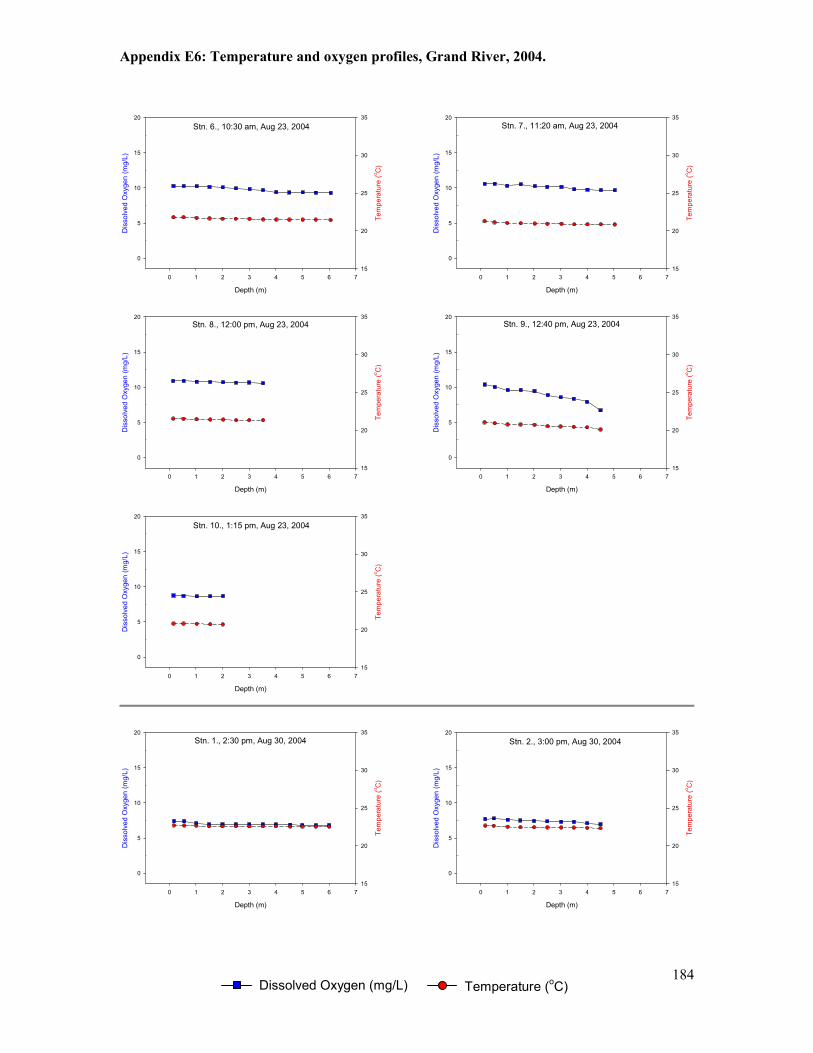
Appendix E6: Temperature and oxygen profiles, Grand River, 2004.
Temperature (oC)Dissolved Oxygen (mg/L)
184
Stn. 6., 10:30 am, Aug 23, 2004
Depth (m)
0 1 2 3 4 5 6 7
Dis
so
lve
d O
xyge
n (
mg/L
)
0
5
10
15
20
Te
mp
era
ture
(oC
)
15
20
25
30
35
Stn. 8., 12:00 pm, Aug 23, 2004
Depth (m)
0 1 2 3 4 5 6 7
Dis
so
lve
d O
xyge
n (
mg/L
)
0
5
10
15
20
Te
mp
era
ture
(oC
)
15
20
25
30
35
Stn. 10., 1:15 pm, Aug 23, 2004
Depth (m)
0 1 2 3 4 5 6 7
Dis
so
lve
d O
xyge
n (
mg/L
)
0
5
10
15
20
Te
mp
era
ture
(oC
)
15
20
25
30
35
Stn. 7., 11:20 am, Aug 23, 2004
Depth (m)
0 1 2 3 4 5 6 7
Dis
so
lve
d O
xyge
n (
mg/L
)
0
5
10
15
20
Te
mp
era
ture
(oC
)
15
20
25
30
35
Stn. 9., 12:40 pm, Aug 23, 2004
Depth (m)
0 1 2 3 4 5 6 7
Dis
so
lve
d O
xyge
n (
mg/L
)
0
5
10
15
20
Te
mp
era
ture
(oC
)
15
20
25
30
35
Stn. 1., 2:30 pm, Aug 30, 2004
Depth (m)
0 1 2 3 4 5 6 7
Dis
so
lve
d O
xyge
n (
mg/L
)
0
5
10
15
20
Te
mp
era
ture
(oC
)
15
20
25
30
35
Stn. 2., 3:00 pm, Aug 30, 2004
Depth (m)
0 1 2 3 4 5 6 7
Dis
so
lve
d O
xyge
n (
mg/L
)
0
5
10
15
20
Te
mp
era
ture
(oC
)
15
20
25
30
35

Appendix E6: Temperature and oxygen profiles, Grand River, 2004.
Temperature (oC)Dissolved Oxygen (mg/L)
185
Stn. 3., 3:30 pm, Aug 30, 2004
Depth (m)
0 1 2 3 4 5 6 7
Dis
so
lve
d O
xyge
n (
mg/L
)
0
5
10
15
20
Te
mp
era
ture
(oC
)
15
20
25
30
35
Stn. 6., 10:50 am, Aug 30, 2004
Depth (m)
0 1 2 3 4 5 6 7
Dis
so
lve
d O
xyge
n (
mg/L
)
0
5
10
15
20
Te
mp
era
ture
(oC
)
15
20
25
30
35
Stn. 8., 1:10 pm, Aug 30, 2004
Depth (m)
0 1 2 3 4 5 6 7
Dis
so
lve
d O
xyge
n (
mg/L
)
0
5
10
15
20
Te
mp
era
ture
(oC
)
15
20
25
30
35
Stn. 10., 12:15 pm, Aug 30, 2004
Depth (m)
0 1 2 3 4 5 6 7
Dis
so
lve
d O
xyge
n (
mg/L
)
0
5
10
15
20
Te
mp
era
ture
(oC
)
15
20
25
30
35
Stn. 5., 10:15 am, Aug 30, 2004
Depth (m)
0 1 2 3 4 5 6 7
Dis
so
lve
d O
xyge
n (
mg/L
)
0
5
10
15
20
Te
mp
era
ture
(oC
)
15
20
25
30
35
Stn. 7., 11:30 am, Aug 30, 2004
Depth (m)
0 1 2 3 4 5 6 7
Dis
so
lve
d O
xyge
n (
mg/L
)
0
5
10
15
20
Te
mp
era
ture
(oC
)
15
20
25
30
35
Stn. 9., 12:50 pm, Aug 30, 2004
Depth (m)
0 1 2 3 4 5 6 7
Dis
so
lve
d O
xyge
n (
mg/L
)
0
5
10
15
20
Te
mp
era
ture
(oC
)
15
20
25
30
35

Appendix E6: Temperature and oxygen profiles, Grand River, 2004.
Temperature (oC)Dissolved Oxygen (mg/L)
186
Stn. 1., 3:30 pm, Sept. 10, 2004
Depth (m)
0 1 2 3 4 5 6 7
Dis
so
lve
d O
xyge
n (
mg/L
)
0
5
10
15
20
Te
mp
era
ture
(oC
)
15
20
25
30
35
Stn. 3., 2:50 pm, Sept. 10, 2004
Depth (m)
0 1 2 3 4 5 6 7
Dis
so
lve
d O
xyge
n (
mg/L
)
0
5
10
15
20
Te
mp
era
ture
(oC
)
15
20
25
30
35
Stn. 6., 11:40 am, Sept. 10, 2004
Depth (m)
0 1 2 3 4 5 6 7
Dis
so
lve
d O
xyge
n (
mg/L
)
0
5
10
15
20
Te
mp
era
ture
(oC
)
15
20
25
30
35
Stn. 8., 1:10 pm, Sept 10, 2004
Depth (m)
0 1 2 3 4 5 6 7
Dis
so
lve
d O
xyge
n (
mg/L
)
0
5
10
15
20
Te
mp
era
ture
(oC
)
15
20
25
30
35
Stn. 2., 4:15 pm, Sept 10, 2004
Depth (m)
0 1 2 3 4 5 6 7
Dis
so
lve
d O
xyge
n (
mg/L
)
0
5
10
15
20
Te
mp
era
ture
(oC
)
15
20
25
30
35
Stn. 5., 11:00 am, Sept. 10, 2004
Depth (m)
0 1 2 3 4 5 6 7
Dis
so
lve
d O
xyge
n (
mg/L
)
0
5
10
15
20
Te
mp
era
ture
(oC
)
15
20
25
30
35
Stn. 7., 12:30 pm, Sept 10, 2004
Depth (m)
0 1 2 3 4 5 6 7
Dis
so
lve
d O
xyge
n (
mg/L
)
0
5
10
15
20
Te
mp
era
ture
(oC
)
15
20
25
30
35
Stn. 9., 1:40 pm, Sept 10, 2004
Depth (m)
0 1 2 3 4 5 6 7
Dis
so
lve
d O
xyge
n (
mg/L
)
0
5
10
15
20
Te
mp
era
ture
(oC
)
15
20
25
30
35

Appendix E6: Temperature and oxygen profiles, Grand River, 2004.
Temperature (oC)Dissolved Oxygen (mg/L)
187
Stn. 10., 2:10 pm, Sept 10, 2004
Depth (m)
0 1 2 3 4 5 6 7
Dis
so
lve
d O
xyge
n (
mg/L
)
0
5
10
15
20
Te
mp
era
ture
(oC
)
15
20
25
30
35
Stn. 1., 10:00 am, Sept. 23, 2004
Depth (m)
0 1 2 3 4 5 6 7
Dis
so
lve
d O
xyge
n (
mg/L
)
0
5
10
15
20
Te
mp
era
ture
(oC
)
15
20
25
30
35
Stn. 3., 11:00 am, Sept. 23, 2004
Depth (m)
0 1 2 3 4 5 6 7
Dis
so
lve
d O
xyge
n (
mg/L
)
0
5
10
15
20
Te
mp
era
ture
(oC
)
15
20
25
30
35
Stn. 6., 1:40 pm, Sept. 23, 2004
Depth (m)
0 1 2 3 4 5 6 7
Dis
so
lve
d O
xyge
n (
mg/L
)
0
5
10
15
20
Te
mp
era
ture
(oC
)
15
20
25
30
35
Stn. 2., 10:30 am, Sept 23, 2004
Depth (m)
0 1 2 3 4 5 6 7
Dis
so
lve
d O
xyge
n (
mg/L
)
0
5
10
15
20
Te
mp
era
ture
(oC
)
15
20
25
30
35
Stn. 5., 12:50 pm, Sept. 23, 2004
Depth (m)
0 1 2 3 4 5 6 7
Dis
so
lve
d O
xyge
n (
mg/L
)
0
5
10
15
20
Te
mp
era
ture
(oC
)15
20
25
30
35
Stn. 7., 2:30 pm, Sept 23, 2004
Depth (m)
0 1 2 3 4 5 6 7
Dis
so
lve
d O
xyge
n (
mg/L
)
0
5
10
15
20
Te
mp
era
ture
(oC
)
15
20
25
30
35

Appendix E6: Temperature and oxygen profiles, Grand River, 2004.
Temperature (oC)Dissolved Oxygen (mg/L)
188
Stn. 8., 3:10 pm, Sept 23, 2004
Depth (m)
0 1 2 3 4 5 6 7
Dis
so
lve
d O
xyge
n (
mg/L
)
0
5
10
15
20
Te
mp
era
ture
(oC
)
15
20
25
30
35
Stn. 10., 4:20 pm, Sept 23, 2004
Depth (m)
0 1 2 3 4 5 6 7
Dis
so
lve
d O
xyge
n (
mg/L
)
0
5
10
15
20
Te
mp
era
ture
(oC
)
15
20
25
30
35
Stn. 9., 3:50 pm, Sept 23, 2004
Depth (m)
0 1 2 3 4 5 6 7
Dis
so
lve
d O
xyge
n (
mg/L
)
0
5
10
15
20
Te
mp
era
ture
(oC
)
15
20
25
30
35
Stn. 1., 3:30 pm, Oct. 5, 2004
Depth (m)
0 1 2 3 4 5 6 7
Dis
so
lve
d O
xyge
n (
mg/L
)
0
5
10
15
20
Te
mp
era
ture
(oC
)
10
15
20
25
30
35
Stn. 3., 4:40 pm, Oct 5, 2004
Depth (m)
0 1 2 3 4 5 6 7
Dis
so
lve
d O
xyge
n (
mg/L
)
0
5
10
15
20
Te
mp
era
ture
(oC
)
15
20
25
30
35
Stn. 2., 4:15 pm, Oct 5, 2004
Depth (m)
0 1 2 3 4 5 6 7
Dis
so
lve
d O
xyge
n (
mg/L
)
0
5
10
15
20
Te
mp
era
ture
(oC
)
15
20
25
30
35
Stn. 5., 2:00 pm, Oct. 5, 2004
Depth (m)
0 1 2 3 4 5 6 7
Dis
so
lve
d O
xyge
n (
mg/L
)
0
5
10
15
20
Te
mp
era
ture
(oC
)
15
20
25
30
35

Appendix E6: Temperature and oxygen profiles, Grand River, 2004.
Temperature (oC)Dissolved Oxygen (mg/L)
189
Stn. 6., 1:30 pm, Oct. 5, 2004
Depth (m)
0 1 2 3 4 5 6 7
Dis
so
lve
d O
xyge
n (
mg/L
)
0
5
10
15
20
Te
mp
era
ture
(oC
)
15
20
25
30
35
Stn. 8., 12:00 pm, Oct 5, 2004
Depth (m)
0 1 2 3 4 5 6 7
Dis
so
lve
d O
xyge
n (
mg/L
)
0
5
10
15
20
Te
mp
era
ture
(oC
)
15
20
25
30
35
Stn. 10., 11:00 am, Oct 5, 2004
Depth (m)
0 1 2 3 4 5 6 7
Dis
so
lve
d O
xyge
n (
mg/L
)
0
5
10
15
20
Te
mp
era
ture
(oC
)
15
20
25
30
35
Stn. 7., 12:40 pm, Oct 5, 2004
Depth (m)
0 1 2 3 4 5 6 7
Dis
so
lve
d O
xyge
n (
mg/L
)
0
5
10
15
20
Te
mp
era
ture
(oC
)
15
20
25
30
35
Stn. 9., 11:30 am, Oct 5, 2004
Depth (m)
0 1 2 3 4 5 6 7
Dis
so
lve
d O
xyge
n (
mg/L
)
0
5
10
15
20
Te
mp
era
ture
(oC
)
15
20
25
30
35
Stn. 1., 9:40 am, Oct. 20, 2004
Depth (m)
0 1 2 3 4 5 6 7
Dis
so
lve
d O
xyge
n (
mg/L
)
0
5
10
15
20
Te
mp
era
ture
(oC
)
10
15
20
25
30
35
Stn. 2., 10:15 am, Oct 20, 2004
Depth (m)
0 1 2 3 4 5 6 7
Dis
so
lve
d O
xyge
n (
mg/L
)
0
5
10
15
20
Te
mp
era
ture
(oC
)
10
15
20
25
30
35
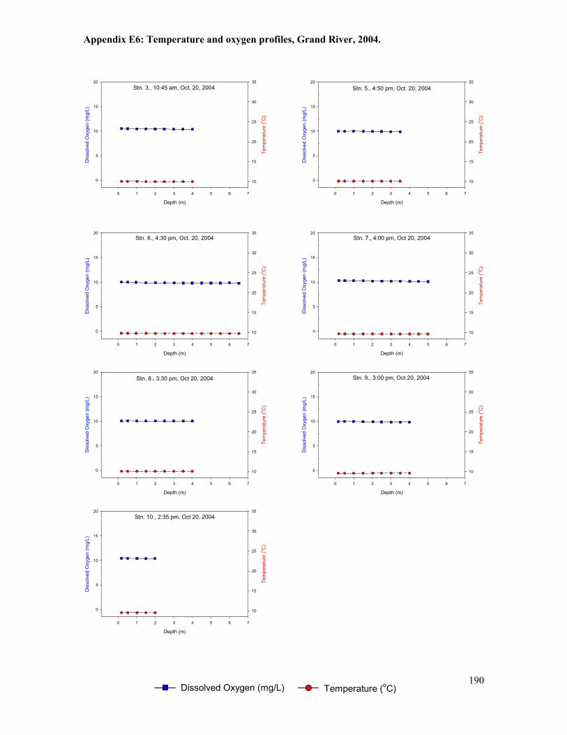
Appendix E6: Temperature and oxygen profiles, Grand River, 2004.
Temperature (oC)Dissolved Oxygen (mg/L)
190
Stn. 3., 10:45 am, Oct. 20, 2004
Depth (m)
0 1 2 3 4 5 6 7
Dis
so
lve
d O
xyge
n (
mg/L
)
0
5
10
15
20
Te
mp
era
ture
(oC
)
10
15
20
25
30
35
Stn. 5., 4:50 pm, Oct. 20, 2004
Depth (m)
0 1 2 3 4 5 6 7
Dis
so
lve
d O
xyge
n (
mg/L
)
0
5
10
15
20
Te
mp
era
ture
(oC
)
10
15
20
25
30
35
Stn. 6., 4:30 pm, Oct. 20, 2004
Depth (m)
0 1 2 3 4 5 6 7
Dis
so
lve
d O
xyge
n (
mg/L
)
0
5
10
15
20
Te
mp
era
ture
(oC
)
10
15
20
25
30
35
Stn. 8., 3:30 pm, Oct 20, 2004
Depth (m)
0 1 2 3 4 5 6 7
Dis
so
lve
d O
xyge
n (
mg/L
)
0
5
10
15
20
Te
mp
era
ture
(oC
)
10
15
20
25
30
35
Stn. 10., 2:35 pm, Oct 20, 2004
Depth (m)
0 1 2 3 4 5 6 7
Dis
so
lve
d O
xyge
n (
mg/L
)
0
5
10
15
20
Te
mp
era
ture
(oC
)
10
15
20
25
30
35
Stn. 7., 4:00 pm, Oct 20, 2004
Depth (m)
0 1 2 3 4 5 6 7
Dis
so
lve
d O
xyge
n (
mg/L
)
0
5
10
15
20
Te
mp
era
ture
(oC
)
10
15
20
25
30
35
Stn. 9., 3:00 pm, Oct 20, 2004
Depth (m)
0 1 2 3 4 5 6 7
Dis
so
lve
d O
xyge
n (
mg/L
)
0
5
10
15
20
Te
mp
era
ture
(oC
)
10
15
20
25
30
35

Appendix E7: Temperature and oxygen profiles, Grand River, 2005.
Temperature (oC)Dissolved Oxygen (mg/L)
191
Stn. 1., 9:00 am, June 15, 2005
Depth (m)
0 1 2 3 4 5 6 7
Dis
so
lve
d O
xyg
en
(m
g/L
)
0
5
10
15
20
Te
mp
era
ture
(oC
)
15
20
25
30
35
Stn. 3., 10:15 am, June 15, 2005
Depth (m)
0 1 2 3 4 5 6 7
Dis
so
lve
d O
xyge
n (
mg/L
)
0
5
10
15
20
Te
mp
era
ture
(oC
)
15
20
25
30
35
Stn. 7., 2:00 pm, June 15, 2005
Depth (m)
0 1 2 3 4 5 6 7
Dis
so
lve
d O
xyge
n (
mg/L
)
0
5
10
15
20
Te
mp
era
ture
(oC
)
15
20
25
30
35
Stn. 9., 3:15 pm, June 15, 2005
Depth (m)
0 1 2 3 4 5 6 7
Dis
so
lve
d O
xyge
n (
mg/L
)
0
5
10
15
20
Te
mp
era
ture
(oC
)
15
20
25
30
35
Stn. 2., 9:40 am, June 15, 2005
Depth (m)
0 1 2 3 4 5 6 7
Dis
so
lve
d O
xyg
en
(m
g/L
)
0
5
10
15
20
Te
mp
era
ture
(oC
)
15
20
25
30
35
Stn. 6., 1:20 pm, June 15, 2005
Depth (m)
0 1 2 3 4 5 6 7
Dis
so
lve
d O
xyge
n (
mg/L
)
0
5
10
15
20
Te
mp
era
ture
(oC
)
15
20
25
30
35
Stn. 8., 2:45 pm, June 15, 2005
Depth (m)
0 1 2 3 4 5 6 7
Dis
so
lve
d O
xyge
n (
mg/L
)
0
5
10
15
20
Te
mp
era
ture
(oC
)
15
20
25
30
35
Stn. 10., 3:50 pm, June 15, 2005
Depth (m)
0 1 2 3 4 5 6 7
Dis
so
lve
d O
xyge
n (
mg/L
)
0
5
10
15
20
Te
mp
era
ture
(oC
)
15
20
25
30
35

Appendix E7: Temperature and oxygen profiles, Grand River, 2005.
Temperature (oC)Dissolved Oxygen (mg/L)
192
Stn. 1., 10:20 am, June 27, 2005
Depth (m)
0 1 2 3 4 5 6 7
Dis
so
lve
d O
xyge
n (
mg/L
)
0
5
10
15
20
Te
mp
era
ture
(oC
)
15
20
25
30
35
Stn. 3., 12:10 pm, June 27, 2005
Depth (m)
0 1 2 3 4 5 6 7
Dis
so
lve
d O
xyge
n (
mg/L
)
0
5
10
15
20
Te
mp
era
ture
(oC
)
15
20
25
30
35
Stn. 6., 10:20 am, June 27, 2005
Depth (m)
0 1 2 3 4 5 6 7
Dis
so
lve
d O
xyg
en
(m
g/L
)
0
5
10
15
20
Te
mp
era
ture
(oC
)
15
20
25
30
35
Stn. 8., 4:30 pm, June 27, 2005
Depth (m)
0 1 2 3 4 5 6 7
Dis
so
lve
d O
xyge
n (
mg/L
)
0
5
10
15
20
Te
mp
era
ture
(oC
)
15
20
25
30
35
Stn. 2., 11:20 am, June 27, 2005
Depth (m)
0 1 2 3 4 5 6 7
Dis
so
lve
d O
xyge
n (
mg/L
)
0
5
10
15
20
Te
mp
era
ture
(oC
)
15
20
25
30
35
Stn. 5., 2:10 pm, June 27, 2005
Depth (m)
0 1 2 3 4 5 6 7
Dis
so
lve
d O
xyge
n (
mg/L
)
0
5
10
15
20
25
Te
mp
era
ture
(oC
)
15
20
25
30
35
Stn. 7., 3:50 pm, June 27, 2005
Depth (m)
0 1 2 3 4 5 6 7
Dis
so
lve
d O
xyge
n (
mg/L
)
0
5
10
15
20
25
30
Te
mp
era
ture
(oC
)
15
20
25
30
35
Stn. 9., 5:00 pm, June 27, 2005
Depth (m)
0 1 2 3 4 5 6 7
Dis
so
lve
d O
xyge
n (
mg/L
)
0
5
10
15
20
Te
mp
era
ture
(oC
)
15
20
25
30
35

Appendix E7: Temperature and oxygen profiles, Grand River, 2005.
Temperature (oC)Dissolved Oxygen (mg/L)
193
Stn. 10., 5:35 pm, June 27, 2005
Depth (m)
0 1 2 3 4 5 6 7
Dis
so
lve
d O
xyge
n (
mg/L
)
0
5
10
15
20
Te
mp
era
ture
(oC
)
15
20
25
30
35
Stn. 1., 9:20 am, July 12, 2005
Depth (m)
0 1 2 3 4 5 6 7
Dis
so
lve
d O
xyge
n (
mg/L
)
0
5
10
15
20
Te
mp
era
ture
(oC
)
15
20
25
30
35
Stn. 3., 11:00 am, July 12, 2005
Depth (m)
0 1 2 3 4 5 6 7
Dis
so
lve
d O
xyge
n (
mg/L
)
0
5
10
15
20
Te
mp
era
ture
(oC
)
15
20
25
30
35
Stn. 6., 6:00 pm, July 12, 2005
Depth (m)
0 1 2 3 4 5 6 7
Dis
so
lve
d O
xyg
en
(m
g/L
)
0
5
10
15
20
Te
mp
era
ture
(o
C)
15
20
25
30
35
Stn. 2., 10:20 am, July 12, 2005
Depth (m)
0 1 2 3 4 5 6 7
Dis
so
lve
d O
xyge
n (
mg/L
)
0
5
10
15
20
Te
mp
era
ture
(oC
)
15
20
25
30
35
Stn. 5., 1:30 pm, July 12, 2005
Depth (m)
0 1 2 3 4 5 6 7
Dis
so
lve
d O
xyge
n (
mg/L
)
0
5
10
15
20
Te
mp
era
ture
(oC
)15
20
25
30
35
Stn. 7., 3:10 pm, July 12, 2005
Depth (m)
0 1 2 3 4 5 6 7
Dis
so
lve
d O
xyge
n (
mg/L
)
0
5
10
15
20
Te
mp
era
ture
(oC
)
15
20
25
30
35
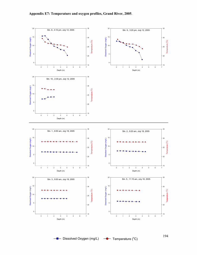
Appendix E7: Temperature and oxygen profiles, Grand River, 2005.
Temperature (oC)Dissolved Oxygen (mg/L)
194
Stn. 8., 4:15 pm, July 12, 2005
Depth (m)
0 1 2 3 4 5 6 7
Dis
so
lve
d O
xyge
n (
mg/L
)
0
5
10
15
20
Te
mp
era
ture
(oC
)
15
20
25
30
35
Stn. 10., 2:30 pm, July 12, 2005
Depth (m)
0 1 2 3 4 5 6 7
Dis
so
lve
d O
xyge
n (
mg/L
)
0
5
10
15
20
Te
mp
era
ture
(oC
)
15
20
25
30
35
Stn. 9., 3:20 pm, July 12, 2005
Depth (m)
0 1 2 3 4 5 6 7
Dis
so
lve
d O
xyge
n (
mg/L
)
0
5
10
15
20
Te
mp
era
ture
(oC
)
15
20
25
30
35
Stn. 1., 8:50 am, July 18, 2005
Depth (m)
0 1 2 3 4 5 6 7
Dis
so
lve
d O
xyge
n (
mg/L
)
0
5
10
15
20
Te
mp
era
ture
(oC
)
15
20
25
30
35
Stn. 3., 9:50 am, July 18, 2005
Depth (m)
0 1 2 3 4 5 6 7
Dis
so
lve
d O
xyge
n (
mg/L
)
0
5
10
15
20
Te
mp
era
ture
(oC
)
15
20
25
30
35
Stn. 2., 9:20 am, July 18, 2005
Depth (m)
0 1 2 3 4 5 6 7
Dis
so
lve
d O
xyge
n (
mg/L
)
0
5
10
15
20
Te
mp
era
ture
(oC
)15
20
25
30
35
Stn. 5., 11:15 am, July 18, 2005
Depth (m)
0 1 2 3 4 5 6 7
Dis
so
lve
d O
xyge
n (
mg/L
)
0
5
10
15
20
Te
mp
era
ture
(oC
)
15
20
25
30
35

Appendix E7: Temperature and oxygen profiles, Grand River, 2005.
Temperature (oC)Dissolved Oxygen (mg/L)
195
Stn. 6., 8:40 am, July 18, 2005
Depth (m)
0 1 2 3 4 5 6 7
Dis
so
lve
d O
xyg
en
(m
g/L
)
0
5
10
15
20
Tem
pe
ratu
re (
oC
)
15
20
25
30
35
Stn. 8., 1:30 pm, July 18, 2005
Depth (m)
0 1 2 3 4 5 6 7
Dis
so
lve
d O
xyge
n (
mg/L
)
0
5
10
15
20
Te
mp
era
ture
(oC
)
15
20
25
30
35
Stn. 10., 2:30 pm, July 18, 2005
Depth (m)
0 1 2 3 4 5 6 7
Dis
so
lve
d O
xyge
n (
mg/L
)
0
5
10
15
20
Te
mp
era
ture
(oC
)
15
20
25
30
35
Stn. 7., 12:50 pm, July 18, 2005
Depth (m)
0 1 2 3 4 5 6 7
Dis
so
lve
d O
xyge
n (
mg/L
)
0
5
10
15
20
Te
mp
era
ture
(oC
)
15
20
25
30
35
Stn. 9., 2:00 pm, July 18, 2005
Depth (m)
0 1 2 3 4 5 6 7
Dis
so
lve
d O
xyge
n (
mg/L
)
0
5
10
15
20
Te
mp
era
ture
(oC
)
15
20
25
30
35
Stn. 1., 8:40 am, July 20, 2005
Depth (m)
0 1 2 3 4 5 6 7
Dis
so
lve
d O
xyge
n (
mg/L
)
0
5
10
15
20
Te
mp
era
ture
(oC
)
15
20
25
30
35
Stn. 2., 9:20 am, July 20, 2005
Depth (m)
0 1 2 3 4 5 6 7
Dis
so
lve
d O
xyge
n (
mg/L
)
0
5
10
15
20
Te
mp
era
ture
(oC
)
15
20
25
30
35

Appendix E7: Temperature and oxygen profiles, Grand River, 2005.
Temperature (oC)Dissolved Oxygen (mg/L)
196
Stn. 3., 9:50 am, July 20, 2005
Depth (m)
0 1 2 3 4 5 6 7
Dis
so
lve
d O
xyge
n (
mg/L
)
0
5
10
15
20
Te
mp
era
ture
(oC
)
15
20
25
30
35
Stn. 6., 8:40 am, July 20, 2005
Depth (m)
0 1 2 3 4 5 6 7
Dis
so
lve
d O
xyg
en
(m
g/L
)
0
5
10
15
20
Te
mp
era
ture
(o
C)
15
20
25
30
35
Stn. 8., 1:30 pm, July 20, 2005
Depth (m)
0 1 2 3 4 5 6 7
Dis
so
lve
d O
xyge
n (
mg/L
)
0
5
10
15
20
Te
mp
era
ture
(oC
)
15
20
25
30
35
Stn. 10., 2:30 pm, July 20, 2005
Depth (m)
0 1 2 3 4 5 6 7
Dis
so
lve
d O
xyge
n (
mg/L
)
0
5
10
15
20
Te
mp
era
ture
(oC
)
15
20
25
30
35
Stn. 5., 11:10 am, July 20, 2005
Depth (m)
0 1 2 3 4 5 6 7
Dis
so
lve
d O
xyge
n (
mg/L
)
0
5
10
15
20
Te
mp
era
ture
(oC
)
15
20
25
30
35
Stn. 7., 12:40 pm, July 20, 2005
Depth (m)
0 1 2 3 4 5 6 7
Dis
so
lve
d O
xyge
n (
mg/L
)
0
5
10
15
20
Te
mp
era
ture
(oC
)
15
20
25
30
35
Stn. 9., 2:00 pm, July 20, 2005
Depth (m)
0 1 2 3 4 5 6 7
Dis
so
lve
d O
xyge
n (
mg/L
)
0
5
10
15
20
Te
mp
era
ture
(oC
)
15
20
25
30
35

Appendix E7: Temperature and oxygen profiles, Grand River, 2005.
Temperature (oC)Dissolved Oxygen (mg/L)
197
Stn. 1., 9:00 am, July 26, 2005
Depth (m)
0 1 2 3 4 5 6 7
Dis
so
lve
d O
xyge
n (
mg/L
)
0
5
10
15
20
Te
mp
era
ture
(oC
)
15
20
25
30
35
Stn. 3., 10:15 am, July 26, 2005
Depth (m)
0 1 2 3 4 5 6 7
Dis
so
lve
d O
xyge
n (
mg/L
)
0
5
10
15
20
Te
mp
era
ture
(oC
)
15
20
25
30
35
Stn. 6., 12:30 pm, July 26, 2005
Depth (m)
0 1 2 3 4 5 6 7
Dis
so
lve
d O
xyge
n (
mg/L
)
0
5
10
15
20
Te
mp
era
ture
(oC
)
15
20
25
30
35
Stn. 8., 1:45 pm, July 26, 2005
Depth (m)
0 1 2 3 4 5 6 7
Dis
so
lve
d O
xyge
n (
mg/L
)
0
5
10
15
20
Te
mp
era
ture
(oC
)
15
20
25
30
35
Stn. 2., 9:50 am, July 26, 2005
Depth (m)
0 1 2 3 4 5 6 7
Dis
so
lve
d O
xyge
n (
mg/L
)
0
5
10
15
20
Te
mp
era
ture
(oC
)
15
20
25
30
35
Stn. 5., 11:25 am, July 26, 2005
Depth (m)
0 1 2 3 4 5 6 7
Dis
so
lve
d O
xyge
n (
mg/L
)
0
5
10
15
20
Te
mp
era
ture
(oC
)
15
20
25
30
35
Stn. 7., 1:10 pm, July 26, 2005
Depth (m)
0 1 2 3 4 5 6 7
Dis
so
lve
d O
xyge
n (
mg/L
)
0
5
10
15
20
Te
mp
era
ture
(oC
)
15
20
25
30
35
Stn. 9., 2:00 pm, July 26, 2005
Depth (m)
0 1 2 3 4 5 6 7
Dis
so
lve
d O
xyge
n (
mg/L
)
0
5
10
15
20
Te
mp
era
ture
(oC
)
15
20
25
30
35

Appendix E7: Temperature and oxygen profiles, Grand River, 2005.
Temperature (oC)Dissolved Oxygen (mg/L)
198
Stn. 10., 2:40 pm, July 26, 2005
Depth (m)
0 1 2 3 4 5 6 7
Dis
so
lve
d O
xyge
n (
mg/L
)
0
5
10
15
20
Te
mp
era
ture
(oC
)
15
20
25
30
35
Stn. 1., 9:10 am, Aug 3, 2005
Depth (m)
0 1 2 3 4 5 6 7
Dis
so
lve
d O
xyge
n (
mg/L
)
0
5
10
15
20
Te
mp
era
ture
(oC
)
15
20
25
30
35
Stn. 3., 10:30 am, Aug 3, 2005
Depth (m)
0 1 2 3 4 5 6 7
Dis
so
lve
d O
xyge
n (
mg/L
)
0
5
10
15
20
Te
mp
era
ture
(oC
)
15
20
25
30
35
Stn. 6., 1:10 pm, Aug 3, 2005
Depth (m)
0 1 2 3 4 5 6 7
Dis
so
lved
Oxyg
en
(m
g/L
)
0
5
10
15
20
Te
mp
era
ture
(oC
)
15
20
25
30
35
Stn. 2., 9:50 am, Aug 3, 2005
Depth (m)
0 1 2 3 4 5 6 7
Dis
so
lve
d O
xyge
n (
mg/L
)
0
5
10
15
20
Te
mp
era
ture
(oC
)
15
20
25
30
35
Stn. 5., 12:40 pm, Aug 3, 2005
Depth (m)
0 1 2 3 4 5 6 7
Dis
so
lve
d O
xyge
n (
mg/L
)
0
5
10
15
20
Te
mp
era
ture
(oC
)15
20
25
30
35
Stn. 7., 2:00 pm, Aug 3, 2005
Depth (m)
0 1 2 3 4 5 6 7
Dis
so
lve
d O
xyge
n (
mg/L
)
0
5
10
15
20
Te
mp
era
ture
(oC
)
15
20
25
30
35

Appendix E7: Temperature and oxygen profiles, Grand River, 2005.
Temperature (oC)Dissolved Oxygen (mg/L)
199
Stn. 8., 2:40 pm, Aug 3, 2005
Depth (m)
0 1 2 3 4 5 6 7
Dis
so
lve
d O
xyge
n (
mg/L
)
0
5
10
15
20
Te
mp
era
ture
(oC
)
15
20
25
30
35
Stn. 10., 3:50 pm, Aug 3, 2005
Depth (m)
0 1 2 3 4 5 6 7
Dis
so
lve
d O
xyge
n (
mg/L
)
0
5
10
15
20
Te
mp
era
ture
(oC
)
15
20
25
30
35
Stn. 9., 3:15 pm, Aug 3, 2005
Depth (m)
0 1 2 3 4 5 6 7
Dis
so
lve
d O
xyge
n (
mg/L
)
0
5
10
15
20
Te
mp
era
ture
(oC
)
15
20
25
30
35
Stn. 1., 9:10 am, Aug 10, 2005
Depth (m)
0 1 2 3 4 5 6 7
Dis
so
lve
d O
xyge
n (
mg/L
)
0
5
10
15
20
Te
mp
era
ture
(oC
)
15
20
25
30
35
Stn. 3., 10:25 am, Aug 10, 2005
Depth (m)
0 1 2 3 4 5 6 7
Dis
so
lve
d O
xyge
n (
mg/L
)
0
5
10
15
20
Te
mp
era
ture
(oC
)
15
20
25
30
35
Stn. 2., 9:45 am, Aug 10, 2005
Depth (m)
0 1 2 3 4 5 6 7
Dis
so
lve
d O
xyge
n (
mg/L
)
0
5
10
15
20
Te
mp
era
ture
(oC
)15
20
25
30
35
Stn. 5., 12:10 pm, Aug 10, 2005
Depth (m)
0 1 2 3 4 5 6 7
Dis
so
lve
d O
xyge
n (
mg/L
)
0
5
10
15
20
Te
mp
era
ture
(oC
)
15
20
25
30
35

Appendix E7: Temperature and oxygen profiles, Grand River, 2005.
Temperature (oC)Dissolved Oxygen (mg/L)
200
Stn. 6., 9:10 am, Aug 10, 2005
Depth (m)
0 1 2 3 4 5 6 7
Dis
so
lve
d O
xyg
en
(m
g/L
)
0
5
10
15
20
Te
mp
era
ture
(oC
)
15
20
25
30
35
Stn. 8., 2:10 pm, Aug 10, 2005
Depth (m)
0 1 2 3 4 5 6 7
Dis
so
lve
d O
xyge
n (
mg/L
)
0
5
10
15
20
Te
mp
era
ture
(oC
)
15
20
25
30
35
Stn. 7., 1:30 pm, Aug 10, 2005
Depth (m)
0 1 2 3 4 5 6 7
Dis
so
lve
d O
xyge
n (
mg/L
)
0
5
10
15
20
Te
mp
era
ture
(oC
)
15
20
25
30
35
Stn. 1., 9:40 am, Aug 15, 2005
Depth (m)
0 1 2 3 4 5 6 7
Dis
so
lve
d O
xyge
n (
mg/L
)
0
5
10
15
20
Te
mp
era
ture
(oC
)
15
20
25
30
35
Stn. 3., 10:45 am, Aug 15, 2005
Depth (m)
0 1 2 3 4 5 6 7
Dis
so
lve
d O
xyge
n (
mg/L
)
0
5
10
15
20
Te
mp
era
ture
(oC
)
15
20
25
30
35
Stn. 2., 10:20 am, Aug 15, 2005
Depth (m)
0 1 2 3 4 5 6 7
Dis
so
lve
d O
xyge
n (
mg/L
)
0
5
10
15
20
Te
mp
era
ture
(oC
)15
20
25
30
35
Stn. 5., 12:40 pm, Aug 15, 2005
Depth (m)
0 1 2 3 4 5 6 7
Dis
so
lve
d O
xyge
n (
mg/L
)
0
5
10
15
20
Te
mp
era
ture
(oC
)
15
20
25
30
35

Appendix E7: Temperature and oxygen profiles, Grand River, 2005.
Temperature (oC)Dissolved Oxygen (mg/L)
201
Stn. 6., 9:40 am, Aug 15, 2005
Depth (m)
0 1 2 3 4 5 6 7
Dis
so
lve
d O
xyge
n (
mg
/L)
0
5
10
15
20
Te
mp
era
ture
(oC
)
15
20
25
30
35
Stn. 8., 2:15 pm, Aug 15, 2005
Depth (m)
0 1 2 3 4 5 6 7
Dis
so
lve
d O
xyge
n (
mg/L
)
0
5
10
15
20
Te
mp
era
ture
(oC
)
15
20
25
30
35
Stn. 10., 3:05 pm, Aug 15, 2005
Depth (m)
0 1 2 3 4 5 6 7
Dis
so
lve
d O
xyge
n (
mg/L
)
0
5
10
15
20
Te
mp
era
ture
(oC
)
15
20
25
30
35
Stn. 7., 1:45 pm, Aug 15, 2005
Depth (m)
0 1 2 3 4 5 6 7
Dis
so
lve
d O
xyge
n (
mg/L
)
0
5
10
15
20
Te
mp
era
ture
(oC
)
15
20
25
30
35
Stn. 9., 2:40 pm, Aug 15, 2005
Depth (m)
0 1 2 3 4 5 6 7
Dis
so
lve
d O
xyge
n (
mg/L
)
0
5
10
15
20
Te
mp
era
ture
(oC
)
15
20
25
30
35
Stn. 1., 8:40 am, Aug 25, 2005
Depth (m)
0 1 2 3 4 5 6 7
Dis
so
lve
d O
xyge
n (
mg/L
)
0
5
10
15
20
Te
mp
era
ture
(oC
)
15
20
25
30
35
Stn. 2., 9:15 am, Aug 25, 2005
Depth (m)
0 1 2 3 4 5 6 7
Dis
so
lve
d O
xyge
n (
mg/L
)
0
5
10
15
20
Te
mp
era
ture
(oC
)
15
20
25
30
35

Temperature (oC)Dissolved Oxygen (mg/L)
202
Stn. 3., 9:40 am, Aug 25, 2005
Depth (m)
0 1 2 3 4 5 6 7
Dis
so
lve
d O
xyge
n (
mg/L
)
0
5
10
15
20
Te
mp
era
ture
(oC
)
15
20
25
30
35
Stn. 6., 1:30 pm, Aug 25, 2005
Depth (m)
0 1 2 3 4 5 6 7
Dis
so
lve
d O
xyge
n (
mg/L
)
0
5
10
15
20
Tem
pe
ratu
re (
oC
)
15
20
25
30
35
Stn. 8., 1:30 pm, Aug 25, 2005
Depth (m)
0 1 2 3 4 5 6 7
Dis
so
lve
d O
xyge
n (
mg/L
)
0
5
10
15
20
Te
mp
era
ture
(oC
)
15
20
25
30
35
Stn. 10., 2:30 pm, Aug 25, 2005
Depth (m)
0 1 2 3 4 5 6 7
Dis
so
lve
d O
xyge
n (
mg/L
)
0
5
10
15
20
Te
mp
era
ture
(oC
)
15
20
25
30
35
Stn. 5., 11:15 am, Aug 25, 2005
Depth (m)
0 1 2 3 4 5 6 7
Dis
so
lve
d O
xyge
n (
mg/L
)
0
5
10
15
20
Te
mp
era
ture
(oC
)
15
20
25
30
35
Stn. 7., 1:00 pm, Aug 25, 2005
Depth (m)
0 1 2 3 4 5 6 7
Dis
so
lve
d O
xyge
n (
mg/L
)
0
5
10
15
20
Te
mp
era
ture
(oC
)
15
20
25
30
35
Stn. 9., 2:00 pm, Aug 25, 2005
Depth (m)
0 1 2 3 4 5 6 7
Dis
so
lve
d O
xyge
n (
mg/L
)
0
5
10
15
20
Te
mp
era
ture
(oC
)
15
20
25
30
35

Temperature (oC)Dissolved Oxygen (mg/L)
203
Stn. 1., 9:10 am, Sep 12, 2005
Depth (m)
0 1 2 3 4 5 6 7
Dis
so
lve
d O
xyge
n (
mg/L
)
0
5
10
15
20
Te
mp
era
ture
(oC
)
15
20
25
30
35
Stn. 3., 10:15 am, Sep 12, 2005
Depth (m)
0 1 2 3 4 5 6 7
Dis
so
lve
d O
xyge
n (
mg/L
)
0
5
10
15
20
Te
mp
era
ture
(oC
)
15
20
25
30
35
Stn. 6., 1:00 pm, Sep 12, 2005
Depth (m)
0 1 2 3 4 5 6 7
Dis
so
lve
d O
xyge
n (
mg/L
)
0
5
10
15
20
Te
mp
era
ture
(oC
)
15
20
25
30
35
Stn. 8., 3:00 pm, Sep 12, 2005
Depth (m)
0 1 2 3 4 5 6 7
Dis
so
lve
d O
xyge
n (
mg/L
)
0
5
10
15
20
Te
mp
era
ture
(oC
)
15
20
25
30
35
Stn. 2., 9:45 am, Sep 12, 2005
Depth (m)
0 1 2 3 4 5 6 7
Dis
so
lve
d O
xyge
n (
mg/L
)
0
5
10
15
20
Te
mp
era
ture
(oC
)
15
20
25
30
35
Stn. 5., 12:20 pm, Sep 12, 2005
Depth (m)
0 1 2 3 4 5 6 7
Dis
so
lve
d O
xyge
n (
mg/L
)
0
5
10
15
20
Te
mp
era
ture
(oC
)
15
20
25
30
35
Stn. 7., 2:20 pm, Sep 12, 2005
Depth (m)
0 1 2 3 4 5 6 7
Dis
so
lve
d O
xyge
n (
mg/L
)
0
5
10
15
20
Te
mp
era
ture
(oC
)
15
20
25
30
35
Stn. 9., 3:30 pm, Sep 12, 2005
Depth (m)
0 1 2 3 4 5 6 7
Dis
so
lve
d O
xyge
n (
mg/L
)
0
5
10
15
20
Te
mp
era
ture
(oC
)
15
20
25
30
35

Temperature (oC)Dissolved Oxygen (mg/L)
204
Stn. 10., 3:55 pm, Sep 12, 2005
Depth (m)
0 1 2 3 4 5 6 7
Dis
so
lve
d O
xyge
n (
mg/L
)
0
5
10
15
20
Te
mp
era
ture
(oC
)
15
20
25
30
35

Appendix E8: Equations describing the relationship between temperature and depth; and oxygen
and depth, during water column profiling on three days, summer, 2005.
205
Temperature at Depth
Station June 27 Temperature slope (m) constant (b) 24 25 27 28
1 y = -1.7999x + 28.572 R2 = 0.9512 -1.800 28.572 2.540 1.985 0.873 0.318
2 y = -1.7026x + 28.772 R2 = 0.9573 -1.703 28.772 2.803 2.215 1.041 0.453
3 y = -1.0654x + 28.101 R2 = 0.8451 -1.065 28.101 3.849 2.911 1.033 0.095
5 y = -2.018x + 29.577 R2 = 0.8267 -2.018 29.577 2.764 2.268 1.277 0.781
6 y = -1.312x + 29.403 R2 = 0.8333 -1.312 29.403 4.118 3.356 1.832 1.069
7 y = -1.3987x + 28.831 R2 = 0.9269 -1.399 28.831 3.454 2.739 1.309 0.594
8 y = -2.3135x + 31.579 R2 = 0.9037 -2.314 31.579 3.276 2.844 1.979 1.547
9 y = -2.1627x + 30.829 R2 = 0.9368 -2.163 30.829 3.158 2.695 1.770 1.308
Average 1-9 3.245 2.627 1.389 0.771
Average 5-9 3.354 2.780 1.633 1.060
ALL Stns y = -1.6702x + 29.387 R2 = 0.8209 -1.670 29.387 3.225 2.627 1.429 0.830
July 12 Temperature m b 24 25 27 28
1 y = -0.9034x + 27.984 R2 = 0.8765 -0.903 27.984 4.410 3.303 1.089 -0.018
2 y = -0.3962x + 27.026 R2 = 0.7653 -0.396 27.026 7.638 5.114 0.066 -2.458
3 y = -0.6178x + 27.358 R2 = 0.9204 -0.618 27.358 5.435 3.817 0.579 -1.039
5 y = -1.2023x + 28.818 R2 = 0.8773 -1.202 28.818 4.007 3.176 1.512 0.680
6 y = -0.8655x + 29.274 R2 = 0.7457 -0.866 29.274 6.094 4.938 2.627 1.472
7 y = -0.5926x + 27.59 R2 = 0.7295 -0.593 27.590 6.058 4.371 0.996 -0.692
8 y = -0.9223x + 28.531 R2 = 0.8361 -0.922 28.531 4.913 3.828 1.660 0.576
9 y = -0.9304x + 28.47 R2 = 0.8739 -0.930 28.470 4.804 3.730 1.580 0.505
Average 1-9 5.420 4.034 1.264 -0.122
Average 5-9 5.175 4.008 1.675 0.508
ALL Stns y = -0.7669x + 28.059 R2 = 0.6992 -0.767 28.059 5.293 3.989 1.381 0.077
August 3 Temperature m b 24 25 27 28
1 y = -0.3901x + 28.122 R2 = 0.8403 -0.390 28.122 10.567 8.003 2.876 0.313
2 y = -0.3838x + 27.784 R2 = 0.8313 -0.384 27.784 9.859 7.254 2.043 -0.563
3 y = -0.4386x + 27.962 R2 = 0.8846 -0.439 27.962 9.033 6.753 2.193 -0.087
5 y = -0.8343x + 27.725 R2 = 0.9632 -0.834 27.725 4.465 3.266 0.869 -0.330
6 y = -0.2463x + 28.109 R2 = 0.9651 -0.495 27.880 7.845 5.823 1.779 -0.243
7 y = -0.8011x + 28.19 R2 = 0.9824 -0.801 28.190 5.230 3.982 1.485 0.237
8 y = -0.8932x + 28.647 R2 = 0.9851 -0.893 28.647 5.203 4.083 1.844 0.724
9 y = -1.3864x + 30.139 R2 = 0.96 -1.386 30.139 4.428 3.707 2.264 1.543
Average 1-9 7.079 5.359 1.919 0.199
Average 5-9 5.434 4.172 1.648 0.386
ALL Stns y = -0.5708x + 28.138 R2 = 0.6897 -0.571 28.138 7.249 5.498 1.994 0.242
Target Temperature (y)

Appendix E8: Equations describing the relationship between temperature and depth; and oxygen
and depth, during water column profiling on three days, summer, 2005.
206
Oxygen at Depth
Station June 27 Oxygen slope (m) constant (b) 5.5 4 2
1 y = -1.9834x + 16.133 R2 = 0.7079 -1.983 16.133 5.361 6.117 7.126
2 y = -3.6524x + 17.753 R2 = 0.9348 -3.652 17.753 3.355 3.765 4.313
3 y = -4.9609x + 20.664 R2 = 0.9332 -4.961 20.664 3.057 3.359 3.762
5 y = -7.4229x + 25.953 R2 = 0.9126 -7.423 25.953 2.755 2.957 3.227
6 y = -4.1527x + 23.572 R2 = 0.9558 -4.153 23.572 4.352 4.713 5.195
7 y = -4.9228x + 22.718 R2 = 0.8485 -4.923 22.718 3.498 3.802 4.209
8 y = -5.2208x + 20.407 R2 = 0.8545 -5.221 20.407 2.855 3.143 3.526
9 y = -4.2499x + 18.698 R2 = 0.9383 -4.250 18.698 3.105 3.458 3.929
Average 1-9 3.542 3.914 4.411
Average 5-9 3.313 3.615 4.017
ALL Stns y = -3.8325x + 19.879 R2 = 0.753 -3.835 19.879 3.749 4.140 4.662
July 12 Oxygen m b 5.5 4 2
1 y = -2.5543x + 15.25 R2 = 0.9319 -2.554 15.250 3.817 4.404 5.187
2 y = -1.4645x + 12.55 R2 = 0.8396 -1.465 12.550 4.814 5.838 7.204
3 y = -2.6261x + 12.476 R2 = 0.9597 -2.626 12.476 2.656 3.228 3.989
5 y = -5.2076x + 19.486 R2 = 0.9951 -5.208 19.486 2.686 2.974 3.358
6 y = -3.61x + 20.581 R2 = 0.9718 -3.610 20.581 4.178 4.593 5.147
7 y = -3.2997x + 17.21 R2 = 0.9881 -3.300 17.210 3.549 4.003 4.610
8 y = -2.9124x + 16.456 R2 = 0.9672 -2.912 16.456 3.762 4.277 4.964
9 y = -2.5352x + 14.057 R2 = 0.9153 -2.535 14.057 3.375 3.967 4.756
Average 1-9 3.605 4.161 4.902
Average 5-9 3.510 3.963 4.567
ALL Stns y = -2.7409x + 15.545 R2 = 0.806 -2.741 15.545 3.665 4.212 4.942
August 3 Oxygen m b 24 25 27
1 y = -0.3901x + 28.122 R2 = 0.8403 -0.390 28.122 10.567 8.003 2.876
2 y = -0.3838x + 27.784 R2 = 0.8313 -0.384 27.784 9.859 7.254 2.043
3 y = -0.4386x + 27.962 R2 = 0.8846 -0.439 27.962 9.033 6.753 2.193
5 y = -0.8343x + 27.725 R2 = 0.9632 -0.834 27.725 4.465 3.266 0.869
6 y = -0.2463x + 28.109 R2 = 0.9651 -0.495 27.880 7.845 5.823 1.779
7 y = -0.8011x + 28.19 R2 = 0.9824 -0.801 28.190 5.230 3.982 1.485
8 y = -0.8932x + 28.647 R2 = 0.9851 -0.893 28.647 5.203 4.083 1.844
9 y = -1.3864x + 30.139 R2 = 0.96 -1.386 30.139 4.428 3.707 2.264
Average 1-9 7.079 5.359 1.919
Average 5-9 5.434 4.172 1.648
ALL Stns y = -0.5708x + 28.138 R2 = 0.6897 -0.571 28.138 7.249 5.498 1.994
Target Oxygen Concentration (y)


