April 2011 Lawrence D. Frank Michael J. Greenwald Sarah Kavage Andrew Devlin WA-RD 765.1 Office of Research & Library Services WSDOT Research Report An Assessment of Urban Form and Pedestrian and Transit Improvements as an Integrated GHG Reduction Strategy
Transcript
April 2011Lawrence D. FrankMichael J. GreenwaldSarah KavageAndrew Devlin
WA-RD 765.1
Office of Research & Library Services
WSDOT Research Report
An Assessment of Urban Form and Pedestrian and Transit Improvements as an Integrated GHG Reduction Strategy
Research Report WA-RD 765.1
Research Project Y-10845 Impact Vehicle Miles Traveled through Coordinated Transportation Investments
AN ASSESSMENT OF URBAN FORM AND PEDESTRIAN AND TRANSIT IMPROVEMENTS AS AN INTEGRATED GHG REDUCTION STRATEGY
by
Dr. Lawrence D. Frank (P.I.), Dr. Michael J. Greenwald, Ms. Sarah Kavage, Mr. Andrew Devlin
Urban Design 4 Health, Inc. P.O. Box 85508
Seattle, WA 98145-1508
Washington State Department of Transportation Technical Monitor
Paula Reeves Local Planning Branch Manager
Prepared for
The State of Washington
Department of Transportation Paula J. Hammond, Secretary
April 1, 2011
Disclaimer The contents of this report reflect the views of the author(s), who is (are) responsible for the facts and the accuracy of the data presented herein. The contents do not necessarily reflect the official views or policies of the Washington State Department of Transportation, Federal Highway Administration, or U.S. Department of Transportation [and/or another agency]. This report does not constitute a standard, specification, or regulation.
2. Review of Previous Work......................................................................................................... 7 2.1. Relevant National and International Research..................................................................... 7
2.2. Relevant Research in Washington State .............................................................................. 9
4.2. Final VMT and CO2 Model Results.................................................................................. 25 4.2.1. Model Performance..................................................................................................... 25 4.2.2. Socio-demographic and control variables................................................................... 28 4.2.3. Urban form, sidewalk coverage and transit accessibility variables ............................ 28 4.2.4. Travel time and cost variables .................................................................................... 28
6. Conclusions.............................................................................................................................. 51 6.1. Summary of Research ........................................................................................................ 51
6.2. Technical Refinements and Adjustments........................................................................... 52
6.3. Opportunities for Future Work and Applications .............................................................. 54
EXECUTIVE SUMMARY In the last several years, Washington State has adopted a series of policy goals intended to reduce greenhouse gases (GHGs). Because transportation is one of the state’s largest sources of GHG emissions, the Washington State Department of Transportation (WSDOT) has been asked to identify ways to reduce Vehicle Miles Traveled (VMT) statewide, and subject to a separate set of state-mandated goals for VMT reduction. Other local governments, such as King County and the City of Seattle, have established their own goals. This study is one of the first studies to test the effect of sidewalks on travel patterns and the first we know of to relate sidewalk availability with VMT and GHG emissions. It has long been assumed that a more complete pedestrian network would be associated with more walking. Years of research have established the basic relationship that exist between the built environment and transportation behavior – a walkable, transit-oriented urban form is overall associated with less driving and more walking and transit use. However, few studies have looked at the potential effectiveness of objectively measured pedestrian infrastructure as a strategy to reduce VMT due the lack of consistently collected data on sidewalks and other pedestrian facilities. Recently, several large jurisdictions in King County have developed local sidewalk data layers, creating a new opportunity to look at pedestrian infrastructure alongside other investment and policy strategies associated with reduced VMT and CO2: urban form, transit service and fares, and parking costs. The study relied on travel outcome data from the 2006 PSRC Household Activity Survey, a recent two day travel survey of the 4-county Puget Sound Region. The household-level analysis was restricted to households in King County cities where sidewalk data was already available: over 70 percent of the King County Activity Survey participants drawn from 9 of the most populated cities in King County. The analysis modeled the association of urban form, pedestrian infrastructure, transit service and travel costs on VMT and CO2, while controlling for household characteristics (such as household size, income and number of children) known to influence travel. The results provide early evidence in the potential effectiveness of sidewalks to reduce CO2 and VMT, in addition to a mixed land use pattern, shorter transit travel and wait times, lower transit fares and higher parking costs. Sidewalk completeness was found to be marginally significant (at the 10 percent level) in reducing CO2, and insignificant in explaining VMT. Increasing sidewalk coverage from a ratio of .57 (the equivalent of sidewalk coverage on both sides of 30 percent of all streets) to 1.4 (coverage on both sides of 70 percent of all streets) was estimated to result in a 3.4 percent decrease in VMT and a 4.9 percent decrease in CO2. Land use mix had a significant association with both CO2 and VMT at the 5 percent level. Parking cost had the strongest associations with both VMT and CO2. An increase in parking charges from approximately $0.28 per hour to $1.19 per hour (50th to 75th percentile), resulted in a 11.5 percent decrease in VMT and a 9.9 percent decrease in CO2. The lack of ability to collect sidewalk data from across all of King County limited the study results. The sample population that resulted was lacking in variation and skewed towards the more urban and walkable parts of King County. This contributed to difficulties with
2
multicollinearity in the modeling process, and may have limited the significance of other urban form variables (such as residential density and intersection density) that have been repeatedly associated with travel outcomes in other King County studies. This study is an important first step towards a more complete understanding of how pedestrian investment, urban form, transit service and demand management (pricing) policy can interact to meet the state’s goals for VMT reduction. The inclusion of sidewalk data from across the entire county or region will provide further, and more conclusive insights. Based on the study results, the research team also developed and tested a simple spreadsheet tool that could be used in repeated applications to estimate the potential reduction in CO2 and VMT due to urban form, sidewalk coverage, transit service and travel cost changes. The spreadsheet could be used in a number of contexts where scenario analysis or impact assessment is appropriate – for example, comprehensive or neighborhood planning, transit-oriented development, or transit corridor planning. The tool was applied in three scenarios in two Seattle neighborhoods – Bitter Lake and Rainier Beach. Rainier Beach is the location of a new light rail (LRT) stop, while Bitter Lake is along a forthcoming bus rapid transit (BRT) service corridor, and both have a large degree of potential to transition into more walkable, transit supportive areas in the future. The results of the scenario testing indicates that current policy will produce small decreases in VMT and CO2: a nearly 8 percent decrease in VMT, and a 1.65 percent decrease in CO2 for Bitter Lake; and a 6.75 percent decrease in VMT and a 2.2 percent decrease in CO2 for Rainier Beach. These numbers indicate that more investment in pedestrian infrastructure and transit service will almost certainly be needed in order to meet stated goals for VMT and CO2 reduction. A scenario was developed that was focused on VM2 / CO2 reduction – complete sidewalk coverage, decreases in transit travel time and cost, and increases in parking costs, and slight adjustments to the mix of land uses. In total, these changes resulted in a 48 percent VMT reduction and a 27.5 percent CO2 reduction for Bitter Lake, and a 27 percent VMT reduction / 16.5 percent CO2 reduction for Rainier Beach – substantial departures from the trend that begin to illustrate what might have to happen in order to reach stated goals for VMT reduction.
3
1. INTRODUCTION & BACKGROUND
1. 1. Problem Statement Land use and transportation research consistently identifies urban form, transit service, and
pedestrian infrastructure as key factors associated with travel behavior characteristics, including
vehicle miles traveled (VMT) and associated greenhouse gas emissions (GHG). In practice,
planners and decision-makers look to a combination of all three strategies in order to create
places that promote walkability and are less reliant on automobile transportation.
Generally, sufficiently complete data on neighborhood urban form characteristics like
density and land use mix, and transit service and regional access are readily accessible or can be
generated at an appropriate analytical scale for many urban regions. Complete city - or region-
wide pedestrian infrastructure data (e.g. sidewalks), however, remains limited in many
jurisdictions, since measurement is time-consuming, non-standardized, and difficult. This has
restricted the available research on pedestrian facilities to ad hoc neighborhood comparisons,
from which it is difficult to generalize broader policy implications. The lack of available
pedestrian infrastructure data has also inhibited integrated analyses with urban form and transit
service variables as related to vehicle use and emission generation.
New sidewalk inventories now available in a number of King County Washington cities,
and the development of detailed estimates of carbon dioxide (CO2) – a major contributor of
greenhouse gas emissions – from transport, have enabled the ability to assess how combined
investments and policy changes could impact non-auto mobility and reduce related GHG
emissions.
4
1. 2. Project Objectives The approved technical aims of this applied research effort were threefold:
1. Develop a method to assess the association between VMT and CO2 emissions and three
principal strategies: a) connectivity and completeness of pedestrian infrastructure; b) urban
form strategies such as compactness of and proximity between complementary land uses, and
levels of street network connectivity; and c) quality of transit service. The analysis will
control for other influences on household VMT and CO2 generation, such as household
sociodemographic characteristics.
2. Analyze the association between the three principal strategies (sidewalk connectivity, urban
form, and transit service) and CO2/VMT. Multiple variables will be tested within each of the
three principal strategies; the final model results will retain only the most important and
effective strategies.
3. Apply the results of the statistical analysis in two neighborhood scale case study locations in
Seattle and generate a comparison between base case or current conditions and one “smarter
growth” alternative. The model will break out the impact of each particular independent
variable on CO2/VMT so that it is possible to see the separate, proportional impact in
CO2/VMT produced by the change in each input variable.
Specific products developed from this research effort include:
1. Elasticity factors, derived from project-specific statistical models, to express how much of a
change in a given outcome (i.e. VMT or CO2) is estimated to be associated with a change in
an independent variable of interest (i.e. urban form, pedestrian facilities, transit service).
Analytical results described in this format provide a readily clear and policy-relevant means
of understanding how general land use decisions and transportation investments may support
5
or detract from VMT and CO2 reduction targets.
2. A predictive analytical tool, developed using project-specific model results, to enable a
flexible and robust evaluation of how alternative development approaches or transportation
investments, particularly at the urban village, neighborhood, or station area scale, impact
vehicle miles traveled and associated levels of carbon dioxide emissions.
1.3. Policy Context Emissions from personal vehicle transport are a large and growing share of total GHG emissions
in Washington. Statewide, the transportation sector currently accounts for approximately 45% of
total GHG emissions, with 73% of these emissions resulting from passenger cars and trucks
fueled by gasoline and diesel1. By 2020, statewide transportation emissions are anticipated to
account for nearly 57% of total emissions2, driven largely by population and employment growth
in urban areas and associated increases in travel demand.
Aggressive GHG reduction targets have been established across many state sectors and
agencies. The adopted 2008 State Climate Change Framework (E2SHB 2815) has set a total
GHG emission reduction target of 50% below 1990 levels by 20503. At the local level, the City
of Seattle Climate Protection Initiative aims to reduce citywide greenhouse gases by 80% below
1990 levels by 20504. Targeted initiatives to help achieve such goals are now central components
of many current policy initiatives. In King County and the larger Puget Sound Region new
Vision 2040 and King County Comprehensive Plan, 2010 Update) are centered around the
prioritization of investments in compact and walkable built environment services by efficient and
accessible public transit and non-motorized networks.
6
Washington State has explicitly legislated the integration of GHG emission targets into
the transportation planning process. Specifically, legislation directs the Washington State
Department of Transportation (WSDOT) to adopt operational goals that reduce per capita VMT
from a baseline of 75 billion annual vehicle miles by 50 percent by 2050, with interim targets of
18 percent by 2020 and 30 percent by 2035 (RCW 47.01.440). Local planning and transportation
agencies are now required to have appropriate capacity to monitor and assess how specific
investments and development initiatives like rail development, corridor planning, and
neighborhood redevelopment may affect emission generation, adversely or otherwise.
WSDOT is in the process of developing the analytical tools and evaluative processes that
will be necessary to address the emission reduction goals with which they are charged. This
includes working together with other state agencies and MTPOs to develop plans and strategies
to meet these goals, pursuant to the Governor’s Executive Order on Climate Change 09-05. This
situation suggests tools and methodologies are needed to help better position state DOTs,
regional MPOs and local governments to assess and monitor the emission implications of
transportation investment and land development decisions.
7
2. REVIEW OF PREVIOUS WORK
2.1. Relevant National and International Research The land use and transportation literature consistently finds multiple urban form, regional
accessibility, and transit service characteristics to be significantly associated with daily travel
behavior outcomes, including VMT.5 Generally, development patterns that 1) concentrate trip
ends (e.g. origins and destinations) within walking and cycling distance to neighborhood
destinations or to transit facilities for regional movement, 2) create a functional mix of land uses
(e.g. live, work, play activities), and 3) have interconnected street networks are consistently and
significantly associated with less driving6, more walking7 and transit use.8 Elasticities between
urban density and VMT on the order of -0.30 have been demonstrated in many studies.9
Significant associations have been observed even after controlling for individual travel and
residential location self-selection attributes and other attitude and preference metrics, suggesting
a certain degree of causality in effect.10,11, 12,13
Travel-related GHG emission reductions associated with compact and walkable built
environment characteristics are potentially significant.14 Ewing et al’s “Growing Cooler” study
suggested that if 60-90 percent of new growth in the United States occurs in compact, walkable,
transit-accessible form, VMT would decrease by 30 percent and nationwide transport-related
CO2 emissions will be reduced by 7-10 percent by 2050, relative to a trend line of continued low-
density, single-use development.15 Growth and development scenarios for 142 U.S. cities
indicate that comprehensive compact development could reduce cumulative emissions by up to
3.2.GtCO2e (or 15-20 percent of projected cumulative emissions) by 2020, in combination with
more efficient vehicles and lower-GHG fuels.16 However, a recent TRB research report found
8
the nationwide GHG impacts of compact development to be much more moderate, with
reductions in CO2 ranging from less than 1 percent to 11 percent in 2050.17 Regional household
location and accessibility measures (e.g. distance and travel times to major population and
employment centers in a region) have been found to exhibit greater magnitudes of effect on
travel-related GHG emissions,18 suggesting that GHG reduction may be best achieved through a
mixture of local and regional investments and actions.
Comprehensive research on the relationship between pedestrian infrastructure and travel-
related outcomes remains limited, largely due to a lack of detailed and objectively measured data
on sidewalk and other pedestrian supportive facilities, which inhibits citywide or region-wide
analysis.19,20 However, several region-wide scale studies that include pedestrian facilities have
recently emerged. An 11-country study of physical activity and the built environment found that
self-reported sidewalk presence was the single biggest factor in influencing physical activity.
People located in urban neighborhoods who report they have sidewalks were between 15-50
percent more likely to get at least 30 minutes of moderate-to-vigorous activity at least five days a
week.21 An increased prevalence of sidewalks was demonstrated to yield the largest “return on
investment” to reduce VMT and increase walking and cycling in Dane County, Wisconsin.22
Taken collectively, urban form, regional and transit accessibility, and pedestrian
infrastructure characteristics all exhibit a significant degree of effect on VMT and CO2 across a
number of studies. These factors are often highly correlated with one another: where urban form
is more pedestrian-friendly, there are often higher-quality pedestrian facilities and better transit
service.23,24 Because this multicollinearity between variables that are included in the same
predictive model may produce large confidence intervals and inappropriately signed coefficients,
composite measures of neighborhood “walkability”25,26 or “accessibility”27 that integrate
9
multiple built environment factors into a single score or measure have been developed and
applied in previous research. However, these strategies eliminate the possibility of analyzing the
effects of individual components of an index (e.g. comparing the effectiveness of land use mix
vs. the effectiveness of residential density), limiting the direct policy-relevance of many research
findings.
2.2. Relevant Research in Washington State The consultant team (Urban Design 4 Health, or UD4H) has been involved in several projects
looking at VMT and CO2 generation from household travel in the King County region. UD4H
originally modeled CO2 emissions from transport as part of the LUTAQH (Land Use,
Transportation, Air Quality and Health) study, which examined the influence of urban form on
CO2 from transport. 28 HealthScape, the follow-up study to LUTAQH, updated these findings
and integrated them into an existing scenario planning model called I-PLACE3S.29 In June 2009,
the consultant team, with support the Puget Sound Clean Air Agency and the Center for Clean
Air Policy, completed a study under review by the Brookings Institution using King County as a
case study. This study looked at the magnitude of changes in urban form and transit service that
would be necessary to achieve targets for transportation related CO2 emissions 2050, given
improvements in vehicle and fuel technology. The study concluded that large changes in
technology, land use patterns and transit service levels would all be necessary to achieve a high
likelihood of meeting the targets; no single strategy provided enough leverage in itself. 30
Building on these ideas, King County funded the consultant team to develop a model to predict
the mean amount of CO2 emissions from transport per household for each block group in King
County. The results of this work are being used by King County and the City of Seattle in its
10
GHG mitigation and development review process under the State Environmental Policy Act
(SEPA). The research took into account household demographic factors, regional accessibility
(measured by average travel time to 13 regional CBD areas by car and by transit), transit service
(measured by number of bus door openings per block group), and local urban form measures
(measured by residential density, mixture of uses, retail floor area ratio and intersection density
within one kilometer along the travel network from the location of the household).
11
3. RESEARCH APPROACH & PROCEDURES
3.1. Project Approach Figure 3.1 illustrates the process used to fulfill the project aims and objectives. Collection of all
required data sets was based on availability and access from various sources. Advanced
multivariate statistical models were developed and tested to determine the type and magnitude of
associations between specified independent variables and VMT and CO2 outcome measures.
Data development and analysis phases were performed in an iterative manner, with model
performance guiding the generation of informative, policy-relevant variables to be tested. A
predictive spreadsheet tool was created for application in assessing VMT and CO2 outcomes of
different development scenarios in the King County region based on the final model results. Two
sample case study areas in the City of Seattle, and associated future built environment scenarios
for each, were developed to demonstrate and test the performance the predictive analytical tool.
Figure 3.1: Research approach
12
3.2. Core Data Sources
The analysis utilized travel, emissions, and land use data from King County and the Puget Sound
Regional Council. Most of these data sources had already been developed by the consultant team
for the previous work in King County. Five primary data sources formed the basis of the
analysis:
• The Puget Sound Regional Council (PSRC) 2006 Household Activity Survey, provided by
PSRC. This survey was a two consecutive day travel diary of 4,746 households in the four-
county region. The 2,699 King County households, and the 45,000+ trips associated with
those households, provided the outcome data on CO2 and VMT for the analysis. CO2
estimates were developed by the consultant team for previous King County projects and are
summarized in Appendix A of this report.
• Network travel time matrices by bus and single occupancy vehicle (SOV) travel modes,
imputed parking charges and imputed transit fares, for the 2006 four county regional travel
network and transportation analysis zone (TAZ) structure. TAZ and network data was
provided by PSRC and used to develop measures of travel time, transit service and travel
costs used as independent variables in the analysis.
• To develop measures of local transit service, active transit stop and route locations within
King County for the February 2006 and June 2006 time periods were used. These stops
covered all bus routes by King County Metro, Community Transit and Pierce Transit
servicing King County. Using both the February and June datasets accounts for any changes
in transit system accessibility during the PSRC travel survey period. King County GIS Data
Center and Sound Transit provided this transit data.
13
• Land use information for the 1-kilometer street network buffer surrounding each household
location for participants in the PSRC 2006 Household Activity Survey residing within King
County. The parcel data was developed for previous consultant team efforts using parcel-
level land use data provided by the King County Tax Assessor. The parcel data, in
combination with the County’s GIS parcel level land use database, was the primary source of
the urban form measures in the analysis. Data from 2006 were used to match the travel
survey time period.
• Local sidewalk data represented the major new data collection effort for this study. Sidewalk
files for nine municipalities within King County (Bellevue, Bothell, Federal Way, Kent,
Redmond, SeaTac, Seattle, Shoreline and Tukwila), provided by the individual jurisdictions
in response to requests by Washington State Department of Transportation staff. Figure 3.2
illustrates cities for which sidewalk data was provided (city borders are in black hashed lines;
those cities for which sidewalk data was received have green lines within their borders).
Specifics on these data sources and methods used to develop the project’s master sidewalk
database and independent variables to be tested are described in Appendix B of this report.
The final household sample used for the project included only those households within King
County cities for which we received sidewalk data.
14
Figure 3.2: Location of King County sidewalks in project database
15
3.3. Dependent Variables Developed and Tested in Analysis Estimated household vehicle miles traveled (VMT) and carbon dioxide (CO2) per day –
VMT and CO2 emission estimates previously developed by UD4H for all King County
participants in the 2006 PSRC Household Activity Survey were utilized. A detailed overview of
the process used to estimate VMT and CO2 is provided in Appendix A of this report. Briefly,
each reported trip completed using a polluting vehicle mode (e.g. Car, Motorcycle, School Bus,
Taxi and Public Bus) was assigned to the PSRC modeled road network assuming a shortest time
path based on the travel time for the mode and time of day. Trips were then broken into multiple
road segments, or “links”, according to vehicle type. For each modeled road segment of each
trip, CO2 emission levels were assessed based on a vehicle’s travel distance and speed (as
determined by the PSRC travel demand model). Road facility type (arterial, freeway, etc),
capacity, and estimated traffic volume based on the time of day are all taken into account using
the method. Estimates also account for engine temperature (hot vs. cold start) and vehicle
occupancy. Vehicle type and acceleration/deceleration data was unavailable for the estimation
process. Final VMT and CO2 variables were generated by calculating the weighted average daily
VMT and CO2 emissions per each household member, and then summing these averages per
household.
3.4. Independent (Explanatory) Variables Developed and Tested in Analysis Independent variables fall into four general categories: (1) neighborhood urban form measures,
variables for parking and transit fares; and (5) socio-demographic and household characteristics
variables. Each variable category has its own set of assumptions, constraints and methods that go
16
into creating a usable data set on which to base a relevant model.
3.4.1. Neighborhood Urban Form Measures Neighborhood urban form measures were calculated for the area within 1-kilometer (km) street
network-based walk-sheds, or buffers, around each PSRC travel survey household location
included in the final study sample. These neighborhood network buffers were developed by
UD4H for previous projects and research. The buffer represents the area accessible to pedestrians
on the street network within a 6-10 minute walking distance. Figure 3.3 below illustrates a one-
kilometer network buffer around a hypothetical activity location. It also shows the difference
between radial (crow-fly) and network approaches to establishing neighborhood buffers.
Figure 3.3: Measuring neighbourhood urban form.
The urban form measures developed were:
17
Net residential density – A measure of residential compactness measured by dividing the total
number of dwelling units by the total number of acres designated residential within the 1km
network buffer.
Intersection density – An approximation of network connectivity. Calculated by the total
number of intersections divided by the total number of square kilometers within the 1km network
buffer.
Land use mix – This variable represents a mixed-use index measure based on building square
footage of specific land use types. The general formula for calculating the level of land use mix
is:
Land Use Mix = -1*A/(ln(n)) where A=(b1/a)*ln(b1/a) + (b2/a)*ln(b2/a) +…+ (bn/a)*ln(bn/a) a = total square feet of land for all five land uses b1= square ft. of building floor area in land use type b1 b2= square ft. of building floor area in land use type b2 bn= square ft. of building floor area in land use type n A value of zero indicates that all the land within the 1km buffer is dominated by a single land
use; a value of one indicates equal distribution of square footage across all the land use
categories. Two variations on the land use mix variable were generated to maximize statistical
significance and meaningful coefficient values across statistical models.
Variation #1, Land Use Mix (including residential uses), represents a mixed-use index
measure based on building square footage of civic & education, entertainment, office,
residential, and retail uses for the 1km network buffer around household location.
Variation #2, Land Use Mix (excluding residential uses), represents a mixed-use index
18
measure based on building square footage of civic & education, entertainment, office,
and retail uses only for the 1km network buffer around household location. The working
hypothesis was that a variety of non-residential destinations may be of more influence on
household travel behavior than presence of other households.
Other measures of land use mix were also calculated based on 3 and 4 land use types.
Retail floor area ratio - Retail FAR is a ratio of retail building floor area to lot (parcel) area,
and measures of the amount of shopping opportunity there is within walking distance of the
household location. Multi-story buildings with no surface parking typically have FAR values
higher than 1.0, so Retail FAR values higher than 1.0 would be expected in areas with multi-
story commercial development (e.g. downtown central business districts). FAR can also be used
as a suitable proxy measure of the pedestrian environment, because parcels with low FARs (0.1 –
0.3) tend to be single-story auto-oriented retail surrounded by parking. Retail FAR is calculated
using the following formula:
∑ Floor Area for all Retail buildings within 1km Buffer ∑ Lot Area for all Retail buildings within 1km Buffer
3.4.2. Pedestrian infrastructure variables Pedestrian infrastructure variables were also calculated for the area within pre-established 1-
kilometer (km) street network-based buffers around each self-reported household location in the
PSRC 2006 Household Activity Survey.
Sidewalk to street ratio - This variable shows the ratio of total sidewalk length within the 1km
buffer compared to total length of street right of way within the 1km network buffer. A
minimum ratio of 0 means there is no sidewalk coverage in the buffer. The maximum ratio of
19
2.00 means there is total sidewalk coverage throughout the buffer. A ratio measure is employed
to accurately capture the percentage of right-of-way that is traversable by pedestrians. A measure
of total linear feet of sidewalk within the 1 km network buffer was considered but determined to
be too gross a measure on which to identify any substantial magnitude of effect on the dependent
variables.
Signalized intersection density – Calculated by counting the number of signalized intersection
locations within each household buffer, then dividing the result of that count by the buffer area
(square kilometers). In contrast to general intersection density as a measure of street
connectivity, signalized intersection density can serve as a proxy indicator of the ease of street
crossing for pedestrians, as traffic signals are generally positioned on larger, arterial streets.
3.4.3. Transit and regional accessibility measures Number of different transit routes – This variable indicates the number of unique transit routes
served by King County Metro, Sound Transit, Community Transit and/or Pierce Transit for the
active stops within the 1km household buffer. In contrast to transit stops, this variable represents
the variety of unique transit paths within walking distance of the household location.
Jobs / population balance - This variable is a ratio of jobs to population for the census block
group where the household is located. This variable measures the balance between the number of
residents and the number of employees in a census block group, relative to the average ratio of
jobs/housing for all of King County. The formula for calculating the jobs/housing balance index
is:
1 – [ABS (EMP - k*POP)/(jobs + k*POP)]
20
where ABS is the absolute value of the expression in parentheses, k is the regional ratio of jobs
to residents for King County, and EMP and POP are the total block group employment and total
block group population, respectively.
Weighted average of transit in-vehicle time – This variable shows the average transit travel
time (in minutes) from the Traffic Analysis Zones (TAZ) where home is located to all accessible
TAZs within King County, during peak period, by transit. Travel times are estimated from origin
to destination TAZ travel time matrices based on the TAZ 2000 zone system, as provided by
PSRC. A weighted measure is calculated using the following formula: 0.25 x AM Peak Period
Transit In Vehicle Time (Mins) + 0.75 x Mid Day Period Transit In Vehicle Time (Mins). The
weighting was established based on the number of daily peak (6) and off-peak (18) service hours
as designated by King County Metro.
Weighted average of transit wait time – This variable calculates the average wait time (in
minutes) for transit from TAZ where the home is located to all accessible TAZs within King
County, during peak period, by transit. Wait times are estimated from origin to destination TAZ
travel time matrices based on the TAZ 2000 zone system, as provided by PSRC. A weighted
measure is calculated using the following formula: 0.25 x AM Peak Period Transit Wait Time
(Mins) + 0.75 x Mid Day Period Transit Wait Time (Mins).
3.4.4. Cost variables for parking and transit fares Imputed average per-trip household parking charge - An estimate of average per-trip parking
charges (in dollars),for each household in the sample, based on imputed TAZ based charges for
household trips from PSRC network estimates. Imputed charges are applied without regard to
21
any actual charges paid by the travel respondent, or mode taken (e.g., for transit trips, parking
charges are anticipated for what a traveler would have had to pay if the trip had been made as a
single occupancy vehicle trip, based on PSRC estimates of hourly charges in the destination
TAZ).
Imputed average per-trip household transit fare – An estimate of average per-trip transit fare
box charges for each household in the sample, based on imputed TAZ based charges for
household trips from PSRC network estimates. Imputed charges are applied without regard to
any actual charges paid by the travel respondent, or mode taken (e.g., for private vehicle trips,
transit charges are anticipated for what a traveler would have had to pay if the trip had been
made as a transit trip, based on PSRC estimates of fare box charges in place in the destination
TAZ, adjusting for the time period of the trip (i.e., peak or off peak period).
3.4.5. Socio-demographic and control variables Total number of persons in the household – Taken directly from a component file of the PSRC
2006 Household Activity Survey.
Total number of workers in the household - Taken directly from a component file of the
PSRC 2006 Household Activity Survey.
Total number of children age 16 years or younger in the household - The total number of
persons by household identifier with age less than 16 from the PSRC 2006 Household Activity
Survey. Since children cannot independently access a vehicle, serving transportation needs of
children is a potential source of additional household trips, even when controlling for all other
sociodemographic and urban form measures.
22
Number of vehicles per licensed drivers - This variable was calculated by dividing number of
self-reported vehicles per number of licensed drivers in the household from the PSRC 2006
Household Activity Survey. A value of 0 means that there is at least one driver in the household,
but no car associated with the household (e.g., someone who lives downtown, but chooses to use
the bus or bike/walk).
Household income – Represented by a dummy variable (0 or 1) indicating if self-reported
household income from the 2006 PSRC Household Activity Survey was higher than CPI
adjusted King County median income (i.e., $64, 324.44; 1=Above Median, 0=At or Below
Median.
3.5. Database Development Households with complete data on all relevant variables were used in the analyses. Complete
data across all vehicle use and emission outcome measures, neighborhood urban form measures
(including sidewalks), transit and regional accessibility measures, socio-demographic and control
variables were required to develop unbiased statistical models. The limiting factor in developing
the project dataset was the availability of sidewalk data. The PSRC 2006 Household Travel
Survey contains 2,699 King County households distributed across the entire region, reporting
39,297 trips made by a mode for which CO2 emissions were estimated. For this project, complete
sidewalk data was only available for 9 of the most populated cities within King County
comprising 71 percent of survey households within King County. The total number of
household buffers with valid sidewalk data was 2,006. Upon examination of those 2,006 cases, a
source of potential error was identified. Some travel survey participants recorded home locations
23
that which, when plotted, were not strictly within the municipal boundaries of the city that they
identified as their home location. For these 77 records, assigning values of sidewalk length
would be incorrect, because they were not within the municipality in the first place. Therefore,
these 77 records were removed from the data set, leaving a final total of 1,929 eligible
households.
3.6. Statistical Predictive Models Advanced multivariate statistical models were developed and tested to determine the type and
magnitude of associations between specified independent variables and VMT and CO2 outcome
measures described previously. Final predictive statistical models took the form of multivariate
regression equations that produced both unstandardized and standardized coefficients, and
statistical significance scores (i.e., T-scores) to indicate which variables were likely to have a
substantial association with household level VMT and CO2 emissions. Separate models were
specified for VMT and CO2 outcomes in order to determine if variation in type and magnitude of
association and overall model performance was present.
3.7. Tool Development Coefficients and parameters generated from the final statistical models were used to build a
predictive, scenario assessment tool documented in an MS Excel spreadsheet. The spreadsheet
tool contains all necessary information to estimate household-level vehicle use and related CO2
emission outputs per unit of time (e.g. kg/day, metric tons/year, etc) and the 95 percent
confidence interval around each baseline and forecasted estimate.
24
3.8. Case Study Testing Case study neighborhoods were selected by the project’s Technical Advisory Committee, in
collaboration with the consultant team in order to test and demonstrate the application of a VMT-
CO2 predictive analytical tool. A number of potential sites were considered for the case studies.
Priority focus was on identifying locations that met some or all of the following criteria in order
to leverage the most policy utility from application of the predictive tool:
1. Capacity to test changes in the independent variables that are the focus of the study,
including:
• Sidewalk coverage. Since most areas of the City have complete sidewalk coverage, there
were only a few areas where we were able to test significant increases in sidewalk
coverage.
• Transit service. The case study areas identified by WSDOT and the City had either
experienced significant increases in transit service since the 2006 travel survey due to the
addition of light rail transit (LRT), or are expecting increases in transit service due to
forthcoming bus rapid transit (BRT) service.
• Urban form (land use mix, residential density, retail FAR, amount of retail, street
connectivity).
2. Relevance in terms of timing and ability to shed light on a forthcoming policy / planning
decision. The City of Seattle has recently begun the process of updating neighborhood plans
for the urban villages. It is therefore possible for the case study results to inform
neighborhood planning processes.
25
4. STATISTICAL MODEL RESULTS
4.1. Sample Descriptives Summary statistics for the neighborhood urban form measures, pedestrian infrastructure
variables, transit and regional accessibility variables, cost variables for parking and transit fares,
and sociodemographic characteristics measured for the sample population (n=1,929 households)
are presented in Table 4.1. These statistics are assessed relative to the entire set of King County
households within the PSRC Household Activity Survey. The distribution of means and one-
sample T-tests indicate that household respondents in the project sample population are located
in generally more compact, walkable, and centrally situated areas, and travel fewer vehicle miles
than the larger King County sample population.
4.2. Final VMT and CO2 Model Results The final statistical models are Ordinary Least Squares linear regressions, measuring the
influence of household socio-demographic traits, urban form measures, transit accessibility and
monetary costs of travel (i.e., transit fares and parking charges) on daily household travel related
CO2 and VMT. Table 4.2 presents the final, best-fitted models of household-level VMT and CO2
for the sample population.
4.2.1. Model Performance The specified models explain approximately 35.19 percent of the variation in daily household
travel related CO2 generation and 32.23 percent of the variation in daily household VMT
generation, respectively, after accounting for the influence of statistically insignificant variables
26
in the model. This share of variation is common to most planning and transportation research
aimed at assessing travel behavior.
Table 4.1: Descriptive statistics
27
Table 4.2. Final VMT and CO2 model results
28
4.2.2. Socio-demographic and control variables All individual and household-level control variables performed as expected. Households with
more workers, more kids, higher incomes and greater vehicle accessibility all are significantly
associated with greater average daily VMT and CO2 generation. This observation suggests the
models are correctly specified and that included measures are internally valid.
4.2.3. Urban form, sidewalk coverage and transit accessibility variables Model coefficients suggest that more pedestrian-oriented urban form characterized by increased
sidewalk availability and land use mix (greater accessibility to destinations) was associated with
lower daily household CO2 levels and VMT generation. Higher values of land use mix within a 1
km network distance of a person’s home is the only consistently significant urban form variable
associated with reduced VMT and CO2, at the 5 percent threshold of statistical significance. The
VMT and CO2 models included different land use mix variables in order to maximize the
inclusion of statistically significant and policy relevant meaningful coefficients. Sidewalk
coverage reached the 10 percent threshold of significance in the CO2 model, but not the VMT
model. Signalized intersection density and number of transit routes did not reach statistical
significance, but because the retain expected direction of effect on both outcomes and have high
policy relevance, they remain in the final model. Sidewalk coverage was also retained in the
VMT model for the same reasons. These estimated coefficients are the best available
approximation available and any statistical insignificance may be caused by a lack of sufficiently
varied data and/or co-linearity among other variables.
4.2.4. Travel time and cost variables
29
The two travel cost variables – imputed daily parking and transit fares per person – were highly
significant at the 5 percent level in both models. Higher daily parking fees at trip destinations
was negatively associated with VMT and CO2 emission levels. Conversely, higher daily transit
fares may discourage transit use as evident through a positive association with VMT and CO2
emission levels. Longer transit wait and travel times may also lead to increased vehicle use and
related CO2 emission levels, as observed by the significantly positive coefficients of these
variables.
4.3. Elasticities Point elasticities express the marginal degree of change in a dependent variable Y that is
anticipated from a change in a pre-specified value of a particular input variable X, holding all
other inputs constant. The main model results provide an absolute estimate of the existing per
household VMT and CO2 levels in King County, and what these levels are expected to be after a
specific change (or combination of changes) to urban form, pedestrian infrastructure, transit
service, and travel pricing are put in place. The elasticity values provide insight into the
anticipated change in VMT and CO2 levels at particular “cut-points” in each independent
variable. Elasticities, employed in this context, also help to understand the return-on-investment
(ROI) or cost-effectiveness of development decisions relative to VMT and CO2 levels.
The magnitude of effective change associated with a given point elasticity is not constant.
The exact pattern of how the value of point elasticities change is dependent in large part on the
distribution of the input variable X for which the point elasticity is being calculated. Generally,
for normally distributed input data, the rate of change between point elasticities is towards
progressively smaller values. Every input variable X has a low and high end to its distribution in
30
the project sample population. As one gets closer to these extremes, it becomes progressively
more difficult to achieve the same percentage change in outcome variable Y by increasing (or
decreasing) the input variable X of interest. This effect is commonly referred to as “diminishing
marginal returns”. A situation where the rate of change between point elasticities does not get
progressively smaller (e.g. increasing returns) may occur when the distribution of the input
variable is skewed.
Table 4.3 provides the quartile percentage values (25th, 50th and 75th percentile) for all
input variables from the project sample population. Table 4.4 and 4.5 illustrates the marginal
change results for the VMT and CO2 models, respectively, obtained through the point elasticity
calculations using the percentile values.
31
Table 4.3: Data Input Percentiles (n=1,654)
32
Table 4.4: Point elasticities based on households in final VMT model
33
Table 4.5: Point elasticities based on households in final CO2 model (n=1,655)
34
The following observations are noteworthy:
• Parking charges have the highest magnitudes of marginal changes between percentiles in
both the VMT and CO2 models. The greatest degree of marginal change occurs when
parking charges are increased from approximately $0.28 per hour to $1.19 per hour (50th
to 75th percentile, which results in a 11.52 percent decrease in VMT and a 9.92 percent
decrease in CO2). This suggests that parking charge rates generate a substantial
influence on VMT and CO2 only when they reach higher-end rates.
• Transit fares, land use mix and signalized intersection density have similar but less
dramatic effects, as evidenced by their overall lower magnitudes (e.g., 1.34 percent to
2.23 percent elasticities on VMT for transit fare, 2.70 to 3.73 percent for mixed use; 1.01
and 1.19 percent for signalized intersection density). These results highlight that urban
form, while difficult to change in the immediate term, may be an effective
complementary strategy to pricing and transit service when trying to reduce VMT / CO2.
• Diminishing marginal returns are evident in the sidewalk ratio variable. Investments in
sidewalk infrastructure are likely to exceed relative cost effectiveness in terms of VMT
and CO2 outcomes when investment exceeds sidewalk coverage in the 50th percentile. For
the project sample, the 50th percentile is a sidewalk ratio of 1.42, equivalent to full
sidewalk coverage on both sides of 71 percent of the street network. In any project area
where that threshold is not yet met, there may be a cost effective benefit in adding
sidewalks.
35
4.4. Model and Data Limitations
4.4.1. Sample distribution The final model was limited by an inability to generate a complete countywide sidewalk layer.
Cases from the 2006 PSRC Household Activity Survey sampled for this research were
constrained to those respondent households with valid sidewalk data to ensure complete built
environment and accessibility measures across all participants. The project scope of work and
timeframe precluded any primary sidewalk data collection efforts by WSDOT or the consultant
team – it was necessary to rely on local jurisdiction sidewalk data, where it existed. Local
sidewalk data was only available for 9 of 39 incorporated areas within King County, or 71
percent of the King County households in the PSRC travel survey. Summary statistics provided
in Section 4.1. indicated a greater prevalence of more compact, walkable, centrally located, less
auto-dependent areas in the project sample households relative to the entire 2006 PSRC
Household Activity Survey. The development of a regional sidewalk layer – either for King
County or the 4-county Puget Sound Region – would benefit future analyses and planning efforts
that seek to understand potential VMT / GHG impacts of sidewalk investment and other
pedestrian infrastructure. This project provides important early evidence that sidewalks may be a
part of such a VMT / GHG reduction strategy.
4.4.2. Multicollinearity Because it limited the variation in urban form across the study sample, the lack of sidewalk data
also contributed to problems with multicollinearity. Multicollinearity (e.g. co-association)
between variables is already common in research on urban form and travel related outcomes. In
this case, it limited the ability to include many generated variables known to relate with VMT
36
and CO2 emissions in the academic and applied literature. Including variables that exhibit high
degrees of multicollinearity in the same model may result in Type II error, or “false-negative”,
situations where meaningful and statistically significant associations are masked and the null
hypothesis (e.g. no meaningful relationship) is accepted when in fact it should be rejected. The
modeling process entailed multiple iterations of testing different combinations of variables to
determine an informative but well-fitted and appropriately performing final model. Interactive
terms (two-way, co-dependent or synergistic effects of groups of variables) and non-linear
transformation of variables (including logarithm and linear input variables) were tested in an
attempt to improve specific variable and overall performance of VMT and CO2 models.
Interactive terms provided no additional or “value-added” results to the findings. Non-linear
transformations resulted in either substantial losses in explanatory power, reductions/complete
losses of statistical significance of urban form variables, or both. The variables retained in all
final models are considered the “best available” and will enable meaningful and policy-relevant
scenarios to be tested by planners and decision-makers. Nevertheless, future work would do well
to improve on the models submitted here.
The following notable independent variables were dropped from the final statistical
models:
• Net Residential Density: Highly co-linear with many other urban form variables, making
them insignificant or wrongly signed, along with a slight loss in model power.
• Intersection Density: This variable was found to be statistically insignificant across all
model iterations. Several variants of intersection density were also tested (non-signalized
intersection density, non-signalized/overall intersection density ratio, signalized/overall
intersection density ratio, signalized/non-signalized intersection density). Results were either
37
statistically insignificant, or confirmed the underlying conclusion that signalized intersection
density increased CO2/VMT output.
• Household Size: Larger household sizes (e.g. number of individuals residing in a dwelling
unit) are generally associated with increased vehicle travel and related CO2 emissions. This
variable was removed from final VMT and CO2 models because co-linearity with Number of
Workers in Household was resulting in “wrong” direction for this variable. Removing
Household Size resulted in less loss of model power than removing Number of Workers in
Household.
4.4.3. Travel cost charge variables Imputed per-trip household parking charges were generated based on PSRC estimates of an
average hourly charge in the destination TAZ. It is possible, however, that parking charge rates
may vary by street or business area within a given TAZ. The PSRC data did not account for such
variation, and was the only regionally consistent information available.
38
5. APPLICATION OF FINDINGS: SCENARIO ASSESSMENT TOOL AND CASE
STUDIES
5.1. Development of Scenario Assessment Tool A predictive scenario assessment tool was generated from the statistical model coefficients and
parameters, and provides a basic platform for King County planning agencies to evaluate how
different combinations of investment and policy strategies may impact household-level VMT
and travel-related CO2 generation. In its current state, the tool can help to inform planning,
zoning, development review, and transportation investment strategies at the neighborhood, urban
village, or station planning areas. Tool equations are calibrated specifically for the King County
area. The tool is documented in a simple Microsoft Excel spreadsheet that contains all necessary
information to estimate household-level vehicle use and related CO2 emission outputs per unit of
time (e.g. kg/day, metric tons/year, etc) and the 95 percent confidence interval around each
baseline and forecasted scenario estimates. Tool instructions are included in Appendix C of this
report. Results from an assessment of tool performance in two case study planning areas are
presented here.
5.2. Study Area Descriptions Criteria used by the consultant team and project Technical Advisory Committee to select case
study areas to test and demonstrate the performance of the scenario assessment tool are
summarized in Section 3.8. Bitter Lake Village (130th Avenue and Aurora in Seattle, WA) and
Rainier Beach were determined to best meet all identified criteria. Case study areas are
illustrated in Figures 5.1 and 5.2, respectively. Turquoise lines signify the case study boundaries;
39
the red and blue circles signify ¼ and ½ mile distance from the transit station.
Figure 5.1. Bitter Lake Village case study
40
Figure 5.2. Rainier Beach case study
41
Bitter Lake Village (130th Avenue and Aurora) Bitter Lake Urban Village is one of the City of Seattle neighborhood plans being updated in 2010
– 2011, which makes the timing of this case study quite relevant and potentially informative
from a policy perspective. There is a significant amount of potential for change in the urban
form and transit service provision around the 130th BRT station. The street network is quite
disconnected, with a sidewalk network that is largely limited to the major arterial streets. The
area is dominated by auto oriented “strip” retail. The presence of large vacant parcels within the
130th station area creates further opportunities to transition to a more pedestrian friendly transit
hub. Bitter Lake Park and Ingraham High School, both within the catchment areas of the 130th
station area, offer an opportunity to connect residential, commercial recreational and educational
facilities with a more complete sidewalk and / or trail network. The boundary includes single
family residential areas outside the urban village boundary in order to properly represent the
character of the neighborhood and generate reasonable results from testing changes in the area.
Rainier Beach Similar to Bitter Lake, Seattle is initiating a neighborhood plan update process in 2010-2011 for
the Rainier Beach area. The sidewalk network to west of LRT station is quite fragmented, and
low density / auto oriented commercial / warehouse / industrial development along Martin
Luther King, Jr. Way S. close to the Rainier & Henderson LRT station creates the opportunity to
transition to a more compact, mixed and pedestrian friendly station area. With Dunlap
Elementary and Rainier Beach High School to the east of the station area and Rainier Beach pool
and the Chief Sealth Trail nearby, this study area also contains a wide array of land use types and
destinations. The study area boundary is focused on the potential light rail catchment area to the
42
east of the station, avoiding a steep hill to the west which is likely to inhibit potential pedestrian
movement and introduce a factor into the analysis for which we were unable to control
(topography). The proposed boundary includes some of the single family areas that surround the
designated urban village and also extends partially into industrial / auto-oriented commercial
areas south of the station - therefore capturing the most complete picture of the light rail station
catchment area as possible.
5.3. Case Study Scenarios Three scenarios were developed to test the performance of the spreadsheet tool. City of Seattle
staff, with input from WSDOT and the consultant team, provided one “existing conditions”
(current population, urban form, infrastructure, pricing and transit service conditions) scenario
and one “current policy” (anticipated population and employment, and planned urban form,
infrastructure, pricing and transit service characteristics based on current policy and investment
plans) scenario for each neighborhood. The consultant team also developed an additional “VMT-
CO2 reduction” scenario to test the tool’s robustness and to determine the magnitude of
development strategies that might be required to yield substantial reductions in transportation-
related VMT and CO2 emissions. Detailed scenario assumptions are described in Appendix D of
this report.
The Existing Conditions scenario assumed 2006 socioeconomic, built environment, transit
service, and travel cost conditions for both the Bitter Lake and Rainier Beach planning areas, in
order to match the time period of the VMT / CO2 data (the 2006 household survey).
Socioeconomic and demographic characteristics were calculated at the block level using U.S.
Census (2000) with the exception of the “average number of licensed vehicles per driver in the
43
household” which utilized comparable data from the PSRC 2006 Household Activity and Travel
Diary survey. Sociodemographics - household size, number of kids and cars per household, and
income - was assumed to remain constant throughout all three scenarios in order to highlight the
“pure” effects of the policy strategies. Built environment, transit service, and travel pricing
assumptions were provided by City of Seattle for the Existing Conditions and Current Policy
scenarios. UD4H then made adjustments to those assumptions for the VMT / CO2 Reduction
scenario while maintaining employment, population and square footage totals.
Apportioning of information between various geographies was required to develop assumptions
for transit service and cost variables that precisely matched the study area boundaries. The
apportioning process used in these circumstances is described in Appendix E of this report. It is
anticipated that scenario results will be an accurate estimate for the actual population as scenario
development utilized actual observed or reported data for the planning areas.
The assumptions used in each of the scenarios are summarized in the tables below. Numbers in
italics were used in other calculations (for example, the square footage numbers were used to
calculate measures of land use mix).
Table 5.1: Bitter Lake Case Study Assumptions
BITTER LAKE
INPUT FACTORS Existing Conditions Current Policy VMT / CO2
Sidewalk Ratio 0.60 0.99 2 Number of Transit Routes 6 6 6 Jobs/Population Balance Total Employment 2548.20 3748.20 3748.20 Total Population 4062.00 7513.94 7513.94 Average Transit Travel Time 105.68 105.68 100.00 Average Transit Wait Time 12.59 10.07 9 Average hourly parking charge 4.36 4.36 5.00 Average transit trip fare 2.04 2.04 2.00 Number of Households in Planning Area 2236.05 4,136.27 4,136.27
Table 5.2: Rainier Beach case study assumptions
RAINIER BEACH
INPUT FACTORS Existing Conditions Current Policy VMT / CO2
ReductionSignalized Intersection Density 4.10 4.10 4.10 Land Use Mix
Retail Square Footage 61,577 74,705 80,000 Sidewalk Ratio 0.96 1.24 2 Number of Transit Routes 12 10 10 Jobs/Population Balance
Total Employment 402.24 552.24 552.24 Total Population 4614.36 6216.59 6216.59
Average Transit Travel Time 92.27 92.26 90.00 Average Transit Wait Time 8.91 7.128662946 6.5 Average hourly parking charge 4.36 4.36 5.00 Average transit trip fare 2.04 2.04 2.00 Number of Households in Planning 1370.20 1,845.97 1,845.97
5.4. Testing and Calibration Assessment of tool performance and case study results were based on the produced nature and
magnitudes of effect. VMT and CO2 output estimates were required to generally conform to the
nature of effects observed in the statistical modeling process for tool performance to be
considered methodological sound and fit for practical application. For example, tested scenarios
45
developed around the largest changes in urban form, transit service and accessibility, and travel
pricing variables relative to the Existing Conditions scenario would be expected to yield the
lowest per household VMT and CO2 estimates relative to other scenarios with less dramatic
variation in variables.
5.5. Interpretation of Results The spreadsheet tool performed as expected in both the Bitter Lake Village and Rainier Beach
case study planning areas. Results are summarized in Tables 5.3 and 5.4 below. The
contribution of each strategy (input factor) to the total average household VMT and CO2 is
shown in the table, to give an idea of relative strategy effectiveness. All told, the Current Policy
scenario resulted in a nearly 8 percent decrease in VMT, and a 1.65 percent decrease in CO2 for
Bitter Lake. Rainier Beach’s Current Policy scenario decreased VMT by 6.75 percent and CO2
by 2.2 percent. These numbers indicate that more investment in pedestrian infrastructure and
transit service will almost certainly be needed in order to meet future goals for VMT and CO2
reduction. However, because residential density was necessarily eliminated from the model, the
City may realize small additional decreases in CO2 and VMT due to substantial planned
increases in residential density in these study areas. Although the evidence in this study does not
support such a conclusion, past research in this region does indicate that residential density is an
important factor in attempting to reduce auto use. Additionally, the analysis only compares two
different growth scenarios within the same neighborhood of the city. Comparing the population /
employment growth predicted for these study areas against that growth in a more exurban area
less well-served by transit would likely provide more contrast in results. The particular approach
to scenario planning will depend on the particular planning process or decision being made – for
46
example, where to locate growth in a city or a region (in the context of comprehensive or
regional planning) or how a segment of predicted growth should be accommodated (in the
context of neighborhood planning, which was the approach taken here).
The VMT / CO2 Reduction scenarios were able to get much larger reductions in VMT and CO2,
primarily by adjusting transit service and cost variables and assuming complete sidewalk
coverage in both study areas. Although the adjustments are small in total, because they are
large-area averages, they would require large amounts of change in a single area or transit route
– or smaller amounts of change to many areas / routes. However, in the judgment of the
consultant team, they are not unrealistic. Small adjustments were also made to the distribution of
land uses within the planned total square footage estimated by the City of Seattle. In total, these
changes resulted in a 48 percent VMT reduction and a 27.5 percent CO2 reduction for Bitter
Lake, and a 27 percent VMT reduction and 16.5 percent CO2 reduction for Rainier Beach –
substantial departures from the trend that begin to illustrate what might have to happen in order
to reach stated goals for VMT reduction.
47
Table 5.3: Bitter Lake case study results
Existing Conditions Current Policy VMT/ CO2 Reduction BITTER LAKE STUDY AREA RESULTS INPUT FACTORS
Estimated VMT
Estimated CO2 (g)
Estimated VMT
Estimated CO2 (g)
Estimated VMT
Estimated CO2 (g)
Signalized Intersection Density 1.30 492.46 1.30 492.46 1.30 492.46 Land Use Mix -6.39 -2229.27 -6.50 -1,789.21 -8.10 -1,910.20 Sidewalk Ratio -0.73 -441.92 -1.20 -727.05 -2.43 -1,469.38 Number of Transit Routes servicing the area -0.49 -185.31 -0.49 -185.31 -0.49 -185.31
Jobs/Population Balance -2.81 -840.83 -2.71 -809.77 -2.74 -820.21 Average Transit Travel Time 8.84 3447.15 8.84 3,447.15 8.36 3,261.98 Average Transit Wait Time 3.94 1637.57 3.15 1,310.05 2.82 1,170.86 Average hourly parking charge -16.01 -5937.50 -16.01 -5,937.50 -18.35 -6,804.31 Average transit trip fare 21.17 8500.40 21.17 8,500.40 20.74 8,327.60 Household Constant (assuming all other impact factors balance to zero)
Existing Conditions Current Policy VMT / CO2 Reduction RAINIER BEACH STUDY
AREA RESULTS INPUT FACTORS
Estimated VMT
Estimated CO2 (g)
Estimated VMT
Estimated CO2 (g)
Estimated VMT
Estimated CO2 (g)
Signalized Intersection Density 0.78 294.44 0.78 294.44 0.78 294.44 Land Use Mix -4.83 -1,329.54 -5.71 -1,216.62 -6.63 -1,257.97 Sidewalk Ratio -1.17 -705.36 -1.51 -912.05 -2.43 -1,469.38 Number of Transit Routes servicing the area -0.97 -370.63 -0.81 -308.85 -0.81 -308.85
Jobs/Population Balance -0.78 -232.75 -0.78 -233.94 -0.79 -236.59 Average Transit Travel Time 7.72 3,009.67 7.72 3,009.52 7.53 2,935.78 Average Transit Wait Time 2.79 1,159.26 2.23 927.41 2.03 845.62 Average hourly parking charge -16.01 -5,937.50 -16.01 -5,937.50 -18.35 -6,804.31 Average transit trip fare 21.16 8,497.95 21.16 8,497.95 20.74 8,327.60 Household Constant (assuming all other impact factors balance to zero)
5.6. Tool Benefits The spreadsheet tool is considered a “first attempt” at developing a comprehensive VMT and
CO2 assessment tool for King County planning agencies. For a short set of instructions on how
to use the tool, see Appendices C and E; for more details on how data and assumptions were
applied to the tool in the case studies, see Appendix D. Practical advantages of this initial tool
include:
Evidence-based The spreadsheet tool is able to replicate the methodology of the research upon which the travel
and environmental outcomes are based. The tool applies the same built environment
characteristics used in the base analysis, and it can incorporate demographic information that is
important to predicting CO2 and VMT. Data required for scenario inputs are readily available to
and calculable for most planning agencies within King County. This situation better enables
application of the tool county-wide.
Interface and ease of use The MS Excel spreadsheet interface is a standard computing program used within the United
States and is familiar and available to most planning practitioners and decision-makers. Baseline
and future scenario characteristics are inputted within the same MS excel spreadsheet tab, with
associated percentage changes provided for all input and outputs variables. This enables the clear
and transparent display of data and information for tool users and stakeholders. Data input and
any adjustments for future planning scenarios can be completed relatively quickly. This enables
an adaptable range of applications from in-house policy assessments to larger neighborhood or
community workshops where participants are able to revise input values as needed or desired.
50
The tool can help to inform planning, zoning, development review, and transportation investment
strategies at the neighborhood, urban village, or station planning areas.
5.7. Tool Limitations The base data and statistical approaches employed to develop the spreadsheet tool restrict its
application in several ways:
Limitations of base research
The tool is limited by the lack of sidewalk data for the less-walkable areas of King County. This
resulted in a lack of variation in the sample and to an extent impacts the generalizability of the
results. Past studies (without sidewalk data) using the same travel and urban form datasets but
for the whole county showed significant relationships for a broader array of urban form variables
than we found in this “truncated” dataset.31 These studies consistently found multiple urban
form variables such as intersection density, residential density, and retail density / presence, to be
associated with VMT and CO2. The tool, while able to test a number of different policy
strategies, is therefore limited in the urban form strategies that are able to be tested.
Input variable range
VMT and CO2 coefficients obtained from statistical models specified using multiple regression
analysis methods are based on a range of variable values drawn from the project sample of
households. These are listed in Table 4.1. King County planning agencies interested in applying
the spreadsheet tool should not test the effect of input variable values that fall beyond the
minimum and maximum range of variables in the project sample of households.
51
Reduced number of urban form variables An optimally specified model and scenario assessment tool would have included all pertinent
urban form variables known to relate with VMT, CO2 active transportation and transit use
described in Section 3.4.1. These include net residential density, intersection density, and retail
floor area ratio – all characteristics of the built environment that are subject to local planning
policy and regulations. Issues with multicollinearity between the various urban form variables, as
discussed previously, limited the number and type of urban variables retained in the final model
and assessment tool. The tool would benefit from additional work to include a wider variety of
urban forms within the sample – for example, including more rural King County households.
6. CONCLUSIONS
6.1. Summary of Research This project provides new empirical evidence associating multi-scale urban form, pedestrian
infrastructure, transit service and travel cost characteristics to household level VMT and CO2
emissions in the King County area of Washington State. The integration of pedestrian
infrastructure data, specifically sidewalk coverage, is a unique contribution to the field of study
and helped to advance a more complete assessment of these relationships. Statistical model
results demonstrate that travel pricing and demand management strategies yield consistently
large and significant influence on VMT and CO2 generation. Nevertheless, the significance of
variables such as land use mix and sidewalk availability suggest that the success of these
strategies may largely depend on having a local land use and transportation system to promote
alternative mobility options.
Marginal analysis results obtained through elasticity development allowed for the
52
determination of which urban form, transit service and pedestrian infrastructure elements may be
most effective in reducing household VMT and related CO2. As with any policy intended to
meet an objectively measurable outcome, urban form interventions to address CO2 (either
directly or indirectly) are subject to diminishing marginal returns. Understanding whether the
change (and presumed benefit) is worth the cost in public investment, and what degree of public
acceptance exists for the proposal is crucial for developing sound and rational policy and
investment choices. Elasticities and marginal change analyses demonstrated that only moderate
increases in sidewalk infrastructure may be needed to yield significant decreases in VMT and
associated CO2. Conversely, more aggressive and substantial increases in land use mix may be
required before a greater return on investment is realized.
Model results were imported into a scenario assessment tool developed in a Microsoft
Excel spreadsheet interface. Model performance was tested on two case study neighborhoods.
The case study assessments were an informative test. The scenarios tested here are a good “first
step” upon which to build additional planning and evaluative efforts.
6.2. Technical Refinements and Adjustments Several improvements could be made in future work to refine the data, statistical models and
scenario assessment tool utilized and produced as part of this effort:
Additional sidewalk and pedestrian infrastructure data Sidewalk data was only available from nine of the 39 King County jurisdictions for the analysis.
This reduced the total number of households that we were able to include in the analysis (73
percent of the King County travel survey households were able to be included in the analysis),
limited the variability of urban form measures, and hampered the study results. The study team
53
strongly recommends collecting additional sidewalk data and re-running the CO2 analysis. This
would help to address the problems with limited variation in the sample and enhance
applicability of the analysis. It will be crucial to measure CO2 from travel as an outcome in
addition to VMT because the relationship between CO2 and VMT is not 1:1, as is often assumed.
There are, in fact, substantive differences between CO2 and VMT due to speed and hot vs. cold
starts. The research team already has in-hand detailed measures of CO2 from travel (described
in Appendix A), urban form and transit service measures for all of the King County travel survey
households in the PSRC survey, giving such a project a head start in terms of timing and budget.
Emission Adjustments Refinements could be made to increase the precision of the emission estimates. California Air
Resources Board (CARB) speed-based emission factors are readily available and would make it
possible for future work to create speed-sensitive CO2 emissions estimates, as opposed to the flat
rate applied in this analysis. CO2 emission estimates could be made sensitive to vehicle model
year and type. Currently the emission rate applied to every trip (regardless of the vehicle type
used) is based on a regional fleet distribution of 55.4% auto and 44.6 light duty truck. Emission
estimates that were sensitive to vehicle model year and type were not available for this effort. To
provide such estimates would require producing the five times of day look-up tables used in this
analysis for each model year of each vehicle type. Even if only two vehicle types were used
(auto, and light duty truck) then 250 (2 vehicle types*25 model years*5 time of day periods)
tables would need to be produced and applied to the survey data.
Distance Adjustments Additional adjustments could increase the accuracy of the travel distance estimates. This analysis
54
is based on TAZ to TAZ centroid emission amounts, which may not be the actual distance
traveled on the road network or the actual trip path (in the case of trips which would otherwise
bypass the TAZ centroid). In particular, TAZ-based estimates for bus trips (both school and
public buses) and short (intra-TAZ) trips would benefit from a more refined approach to
determining trip distance. In the future, these estimates could be refined by using the point on the
PSRC model road network that is nearest the trip end to calculate distance, rather than the TAZ
centroid, as the base from which to estimate the trip distance in the PSRC model. Network-based
offset distances could also be used, which would not only allow a more accurate approximation
of the travel path, but would allow the further refinement of speeds for each link of that travel
path. This is especially important for intrazonal trips; for those trips, it was necessary to assume
the entire offset distance was traveled at 20mph.
6.3. Opportunities for Future Work and Applications The statistical models and scenario assessment tool developed here are considered a “first step”
towards understanding and measuring the effect of different built environment characteristics
and transportation system investments on household level VMT and CO2 emissions. Future
work would do well to build off this effort through any of the following means:
“Focal points” of change To be most instructive, additional scenarios should be specified to test different focal points of
urban form, pedestrian infrastructure, and transit service and accessibility changes. For example,
a scenario should be specified that is focused on increasing planning area sidewalk coverage and
another focused on increasing transit service availability, while holding all additional variables
constant.
55
Creating a more robust planning tool A more detailed planning tool could be developed based on the results of this work. This might
include more detailed estimation of urban form elasticities and/or diminishing marginal effect of
urban form on VMT/CO2 mitigation. However, it is recommended that the underlying
shortcomings of the analysis (the inclusion of a full set of sidewalk data) are addressed before
further tool development commences.
Build additional street design / pedestrian environment variables Future work could benefit from data collection and development and testing of other more
detailed street design variables. For example, this could include an integrated nonmotorized and
street network, which will better capture the connectivity of the pedestrian environment and
allow the creation of variables that compare pedestrian and vehicle connectivity.
Assess multiple health and environmental outcomes New research suggests that urban form strategies that promote lower rates of VMT yield “win-
win” strategies across environmental and human health outcomes.32,33 Although informative,
many of the studies fail to include micro-scale pedestrian infrastructure variables into their
analyses. Models developed for this research project that include detailed pedestrian
infrastructure information could be re-specified to assess their synergistic effects on both
emission and physical activity or obesity outcomes.
56
7. RECOMMENDATIONS With a projected population increase of nearly half a million additional residents by 2030 (about
a quarter of the current population) there exists significant opportunity to ensure new
development in King County, the Puget Sound Region and statewide supports vehicle use
reductions and lower carbon footprints. Findings from this research provide additional, evidence-
based information to assist the Washington State DOT, King County, and other regional, state
and local planning agencies develop reasonable and defensible climate reduction plans, goals,
and objectives. Moreover, as these entities move forward with implementation of these
strategies, the scenario assessment tool will help to identify and monitor neighborhood growth
and redevelopment initiatives that will result in tangible VMT and CO2 emission reductions.
57
ACKNOWLEDGEMENTS We thank the project managers and the project’s Technical Advisory Committee for the thoughtful guidance they provided throughout this study. Project managers: Kathy Lindquist, Washington State Department of Transportation Paula Reeves, Washington State Department of Transportation Technical Advisory Committee: Christopher Aiken, Washington State Department of Transportation Kristian Koefed, City of Seattle Brian Lagerberg, Washington State Department of Transportation Chad Lynch, City of Seattle Charles Prestrud, Washington State Department of Transportation Jill Simmons, City of Seattle Brennon Staley, City of Seattle
APPENDIX A
Development of VMT/CO2 Outcome Measures
A-1
APPENDIX A: DEVELOPMENT OF VMT/CO2 OUTCOME MEASURES Measuring CO2 Emissions Methods used to estimate CO2 emissions evolved out of methodologies developed for detailed assessments of criteria air pollutants34. The process relied on information about each vehicle trip taken by King County households in the 2006 PSRC travel survey, supplemented by information from the PSRC travel demand model. Each reported trip was assigned to PSRC’s modeled road network assuming a shortest time path based on the travel time for that mode and time of day. Trips were then broken into multiple road segments, or “links” according to facility type. For each modeled road segment of each vehicle trip, CO2 emissions levels were assessed based upon a vehicle’s travel distance and speed. The travel speed on any given segment was determined by PSRC using its travel demand model. The model takes into account road facility type (arterial, freeway, etc), capacity and estimated traffic volume based on the time of day. This approach is a much more detailed measurement than the standard methodology, which uses a simple average speed for each trip and relies on self reported travel time and resulting speed. The PSRC travel survey includes 45,606 trips from King County households. Of that total, 39,297 trips were made by a mode for which CO2 emissions were estimated (car, public bus, school bus, motorcycle and taxi/shuttle. Our emissions estimation used the following main steps, each of which will be discussed in more detail in the sections that follow:
1. Determine travel modes for which emissions estimates will be created, and assign a primary travel mode to each trip.
2. Determine travel path, speed and distance. 3. Calculate CO2 emissions for all modes, and adjust for cold starts and vehicle
occupancy. 1. Determining Travel Mode. PSRC travel survey participants were able to report up to five different modes used to complete their trip. For example, a person could report they went from home to work by driving their car to the ferry terminal, riding the ferry, walking from the ferry terminal to a bus stop and after arriving near their destination by bus walking the rest of the way to their work location. Of the 45,605 trips in the analysis set (trips made by King County households), 96.4% of them reported using a single mode, 2.5% of trips used two modes, 1% of trips used three modes, and 0.1% of trips used four modes. No trips listed 5 or more types of transportation. For this analysis we only estimated CO2 emissions for a single mode per trip – the ‘primary’ mode. For trips where survey respondents reported more than one mode, the following rules were used to determine which mode was the ‘primary’ mode for each trip:
• If a trip used a public bus for any segment of a trip (regardless of other modes used) that trip was categorized as having public bus as its primary mode.
• If a trip used a school bus for any segment of a trip (regardless of other modes used) that trip was categorized as having school bus as its primary mode.
A-2
• If a trip used a car/van/truck for any segment of a trip (regardless of other modes used, unless a public bus or school bus is used) that trip was categorized as having car/van/truck as its primary mode.
• If a trip used a taxi/shuttle for any segment of a trip (regardless of other modes used) that trip was categorized as having taxi/shuttle as its primary mode1.
2. Determining Travel Path, Speed and Distance. The actual trip path followed for each travel survey trip was not recorded in the PSRC travel survey. In order to estimate the trip path, PSRC, using its modeled road network and travel demand model’s equilibrium assignment process, modeled the shortest time-path for the travel survey trips. Traffic volume and flow (congestion levels) were used to determine the shortest time path (from a loaded assignment at equilibrium) depending on the reported time of the trip. In order to determine trip distance, trip origins and destinations were assigned to the centroid (centerpoint) of the TAZ which contained them. For intra-TAZ trips, the TAZ to TAZ centroid distance method was not used, as it would result in a trip distance of zero. Instead, the PSRC model estimates an average intrazonal trip length based on the area of the TAZ2. For the distances associated with intra-zonal trips, we assumed the travel speed was 20 mph for their entire length, and applied the corresponding emission value for that speed. Distance Adjustments. The TAZ-based estimates used in this analysis for vehicle trips provided by PSRC do not account for the distance between the actual trip end point and the TAZ centroid. Most trips do not start or end at the TAZ centroid, but at some other location within the TAZ. However, the centroid is a central location where the major roadway network is located and is designated by the PSRC as the surrogate geographic terminus for trips within a zone because of its ability to provide an “average” approximation of origins and destinations within that zone. Figure A-1 below conveys the origin (O) and destination (D) of a hypothetical trip in relation to the TAZ centroid. It is important to also note that TAZ-based estimates for bus trips (both school and public buses) are quite unlikely to accurately represent the actual path (route) of the bus, since the bus route is unlikely to be the shortest time path between the origin and destination TAZ.
Figure A-1. Trip Path Based on TAZ Centroids and Actual Trip Ends (O and D)
1 Only one taxi trip used another mode (bicycle). 2 http://wwwpsrc.org/data/tdmodel/model_doc(final).pdf (pg. 147: Average-intrazonal-trip-length (in miles) = 0.75 * SQRT (area (in sqmi)). “For a square TAZ, the square root of the area gives the length of one side. For a non-square TAZ, the square root of the area is the side of an equivalent square. The average length of a straight line with both ends randomly chosen in the unit square is 0.52665 if the distance is Pythagorean, 0.67333 if the distance is rectilinear. The coefficient of 0.75 is a higher than it would be for a unit square, but is a reasonable number to use for the wide mix of TAZ shapes.”
A-3
We attempted to adjust the centroid-based trip distances estimates in order to account for distance between the actual trip end point and the TAZ centroid. Using X/Y coordinates of the TAZ centroids and actual trip end locations, it is possible to calculate the crow-fly (straight line) distance between the trip end point and TAZ centroid. This adjustment added, on average, just over a half-mile to the beginning and end of each trip (about 1.1 miles per trip, on average). However, this approach would only have added the distance between the TAZ centroid and the trip end, regardless of the direction of the trip.
The hypothetical trip shown in the figure above (between points O and D) is longer than the distance between TAZ centroids. However, the opposite circumstance also exists where the distance between points O and D is shorter than the distance between the TAZ centroids. Therefore, while adding the calculated distances from the actual trip origins to the centroid would work in the case shown, it would artificially bias the results by always increasing distances and not accounting for the opposite condition, where trip ends are closer than centroids. Because of this we chose to use the centroids and not add in the additional distances between trip ends and centroids. Due to averaging from trips that are longer or shorter than the centroid locations, it is not anticipated that this approach will bias the results. A distinct advantage of the centroid-based approach is that it is consistent with the methods employed by the PSRC for travel demand modeling -- and it is an acceptable industry standard.
Concurrent with this process of determining speeds and distances, PSRC applied California Air Resources Board (CARB) provided speed-based CO2 emissions rates to determine a CO2 emissions amount for each link of each trip based on the estimated travel speed and distance. The amount from all links in the modeled path were summed to give a trip total between TAZ centroids. 1. Calculating Distance and CO2 Emissions. It was not possible to estimate CO2 emissions for all travel modes reported in the PSRC travel survey. In the case of motorcycle trips, there was no ability to use a common emission factor ratio (across all speeds) to adjust the auto/truck emissions provided by PSRC. For public bus and school bus modes emissions were estimated based on the trip distance provided by PSRC in the travel survey data, estimated fuel mileage, and the US Environmental Protection Agency’s
A-4
(EPA) ratio of pounds of CO2 emissions per gallon of diesel fuel (22.2)3. This single conversion factor does not account for speed or acceleration. For auto-bus combination trips it was not possible to proportion the trip distance between the different modes given available survey data. Nonmotorized modes were assigned zero emissions. The remainder of the modes (ferry, golf cart, wheelchair, train) generated emissions, but had very small trip totals and no clear methodology to estimate emissions.
Emissions factors provided by CARB were used to generate CO2 emissions for car/van/truck and taxi/shuttle trips – the vast majority of the trips. These emissions factors account for vehicle acceleration and deceleration, a refinement over factors used in the past. For each time period, the emissions per mile for each link of each trip were calculated and aggregated up to total per-vehicle, per-trip emissions. Vehicle Occupancy. Emissions and distance were divided among vehicle occupants to create a per-person, per-trip total. For auto/van/truck trips we used the vehicle occupancy reported by travel survey participants. The maximum number of people a survey participant could indicate were in the vehicle with them is “6 or more.” When this amount is indicated the number of people in addition to the survey participant that are assumed to be in the vehicle is 6. Ridership data provided by King County Metro Transit was used to apply average weekday ridership assumptions of 11.29 passengers for off peak (midday, night and evening) periods, and 12.59 passengers for peak periods (AM and PM). For school buses we assumed an occupancy of 35, and in the case of taxis vehicle occupancy was assumed to be 1 for the purpose of allocating emissions. Although taxis will have at least 2 people in them, but as in the case of driving alone, the sole reason the trip is occurring is due to a single person, and therefore all the emissions generated were assigned to that person. Household Level Estimates. Once the emissions and distance estimates were apportioned as described above, the per capita values were aggregated to the individual household level, for each day of the two travel diary. These daily aggregated totals were then averaged to create a daily household VMT and GHG emissions estimate, which serve as the dependent variables (i.e., output measures) for this project. The relevant formulae are: Equation 1 Personal Daily Average CO2 Emissions from Travel
where d = Index (the count) of survey days for a specific individual within a household Equation 2 Estimated Household Daily CO2 Emissions from Travel
3 U.S. Environmental Protection Agency. Emissions Facts: Average Carbon Dioxide Emissions Resulting from Gasoline and Diesel Fuel. Accessed February 23, 2011 at <http://www.epa.gov/otaq////////////climate/420f05001.htm>
A-5
where p = Index (the count) of survey participants within a particular household
APPENDIX B
Sidewalk Data Assembly
B‐1
APPENDIX B: SIDEWALK DATA ASSEMBLY 1. Data Generation and Assembly Procedures 1.1. Initial Data Cleaning and Development Preliminary estimates of total sidewalk distance within each household’s 1 km network buffer were calculated by intersecting network buffer polygons around household locations with a master sidewalk line file created for this project. The master sidewalk line file was created by merging together the individual sidewalk files for the nine municipalities in UD4H possession:
• Bellevue • Bothell • Federal Way • Kent • Redmond • SeaTac • Seattle • Shoreline • Tukwila
In order to successfully execute the merge of the line files for the separate municipalities, several initial data cleaning steps had to be performed. The specific tasks with regards to selecting, modifying and validating the data for each municipality varied, but generally involved at least one of the following tasks:
1. Because the sidewalk archives were organized according to the administrative requirements of each jurisdiction, the first step was to identify which common elements could be combined. For example, one jurisdiction (SeaTac) provided only centerlines of streets with sidewalks, with notation within the underlying data table as to which street segments had only one side of the street covered by sidewalks. In two other jurisdictions (Bothell and Federal Way), sidewalk segments were provided as polygons. In this case, including the length of more than one edge of the polygon would grossly overestimate the length of sidewalk surface (see Figure B-1, below).
B‐2
2. The sidewalk elements needed to be selected out from any other elements in the municipal source record which were not immediately relevant to the analysis (e.g., crosswalks, railroad crossings, impervious surfaces, etc.). Details for each municipality is presented in Section 3 of this appendix.
3. The individual sidewalk files had to be reconciled with the date of the travel survey (2006). This was done either by using the existing metadata, or contact with relevant staff members within each municipality (as identified by WSDOT staff).
4. The individual sidewalk files had to share a common geography type (i.e., line or polyline), in order to be consolidated into a single master shapefile.
5. The definition of what constitutes a sidewalk segment (paved, raised right of way, as opposed to simply striped asphalt or gravel) should be consistent across the jurisdictions included in the analysis.
In the final assessment, only the length of sidewalk and geographic location were provided in sufficient detail to be combined across all data sets. Once the individual municipal files were standardized according to these cleaning steps described above, they were consolidated using the Merge tool in ArcGIS 9.3.1 (found under the General directory in Data Management Tools). The specific properties of this consolidated master file can be found in Section 4 of this appendix. The master sidewalk file was then overlaid onto the polygons for the 1 km network buffer around each household location in King County contained in the PSRC 2006 Household Travel Survey (N=2,699). Using the Intersect tool in ArcGIS 9.3.1, the polygons were used to create a subset of the master sidewalk file which calculated the length of each segment of sidewalk intersecting a specific 1 km buffer. These results were then exported to Microsoft Access, and
B‐3
an aggregation query was performed to estimate the total length of all sidewalk segments within 1 km of each household. A similar application of the Intersect tool, and aggregation query was performed on an archived version of the walkable street network for King County, to generate the total distance of pedestrian accessible street right of way within 1 km of each household. The total number of buffers with non-zero total sidewalk distance was 2,006. 1.2. Validity Check Once the total sidewalk and street distances were calculated for the buffers, the last task was a validity check for the cases where no sidewalk distance was returned. Upon examination of the cases, a source of potential error was addressed. Some travel survey participants recorded home locations that which, when plotted, were not strictly within the municipal boundaries of the city that they identified as their home location. For these 77 records, assigning values of zero sidewalk length would be incorrect, because they were not within the municipality in the first place. These records were removed from the data set. Total number of viable cases with sidewalk data: 2,006 – 77= 1,929 Initial Sidewalk Dataset: Summary Statistics and Variable Definitions The current data set contains sidewalk information on the 1 kilometer network buffer area around 1,929 King County household locations that participated in the 2006 Puget Sound Transportation Survey. The variables collected include the total linear feet of sidewalk within each network buffer (accounting for sidewalks on both sides of the street), the total length of walkable streets within each buffer, and the ratio between the two. Except in cases of measurement error, the upper limit of the ratio between total sidewalk distance and total street distance is 2.00; a street segment cannot have more than twice the length of the right of way covered by sidewalks. Of the 1,929 participants currently under consideration, there are 4 cases where the ratio grossly exceeds this 2.00 upper limit; upon closer inspection, the overages appear to be paved paths which extend beyond existing road right of ways for the walkable street subset. Further inspection of these cases will be performed to determine if the observations should be cleaned or removed from consideration. Table B-1 – Sidewalk Data Summary, All Cases
Total linear feet of sidewalk estimated
within the participant network buffer (accounting for both sides of
street)
Total linear feet of walkable street surface
(e.g.,excluding interstate highways and non pedestrian bridges) estimated
Table B-1 provides the mean, median and values at specific percentile cut points for each of these variables, for all cases in the dataset. The average of the total linear sidewalk distance within each 1 km buffer is to 100,655.9 feet (19.06 miles); for total length of walkable street surface, the corresponding values is 77,657.8 feet (18.32 miles), and the ratio average is 1.1557 (i.e., there is, on average, an 15.57% greater amount of total sidewalk distance than street surface within a participant’s 1 km home location network buffer. Put another way, if total sidewalk coverage would is a ratio of 2.00, 1.1557 represents about 60% sidewalk coverage. Figure B-2 charts the mean and median sidewalk ratio values for participant households, grouped by their individual municipalities; more detailed analyses for the individual municipalities can be found in Appendix C.4 These results are included for demonstration purposes only. Figure B-2: Mean and Median Sidewalk Ratio Values for Participants, by Individual
Municipality
4 The number of observations in each percentile grouping are not reported in Appendix C, due to limited sample sizes in most municipalities.
B‐5
0.56
0.82
0.40
0.66
1.63
0.44
1.35
0.45 0.510.55
0.86
0.26
0.60
1.72
0.41
1.54
0.430.50
0.00
0.20
0.40
0.60
0.80
1.00
1.20
1.40
1.60
1.80
2.00
Sidewalk SurfaceRatio Values
Community (with number of participant households)
Mean
Median
The results in Table 2, while informative, illustrate the potential limitation of trying to analyze individual cities with the PSRC 2006 Household Activity and Travel Diary Survey. While the City of Seattle has sufficient sample size to indicate their values are representative for the entire city, smaller cities may not have sufficient sample size. If, for some unknown reason, the observations in Redmond were not representative of the City of Redmond as a whole (e.g., survey participants more prone to pedestrian behaviors in Redmond were more likely to locate in areas which support that travel mode, so they have better sidewalk connectivity within their buffer), then the values would not be representative for City of Redmond as a whole. In contrast, City of Seattle, with a much larger sample size, is more likely to be representative of the city as a whole. 2. Directions for Future Data Assembly Steps While these assessments represent a useful first step, their primary role is to serve as the basis for further data development. Total linear feet of sidewalk is too gross a measure on which to identify a substantial magnitude of effect, and is also highly collinear with total street right of way within the 1 km buffer (R=+0.881 in the sample). Additionally, the ratio is an imperfect measure of the effects of sidewalks on VMT/CO2 generation because the effect on inspiring pedestrian behavior is anticipated to be non-linear (i.e., going from 0 to 1 full side of the street covered with sidewalk surface is expected to be more effective than the additional gain of going from 1 to both sides of the street being covered). In order to account for these effects, we would need to build more refined measures of sidewalk surface within the 1 km buffer area. Specifically, we would have to develop the percentage of walkable street surface within the 1 km buffer which has no sidewalks, sidewalks on one side of the street, and sidewalks on both sides of the street. Measures could also include the percentage of sidewalk coverage along routes to specific destinations (e.g., schools, parks, retail outlets, etc.).
B‐6
3. Sidewalk Data Assembly Metadata Criteria Selection Notes Bellevue—Data structure made it difficult to discern different types of non-motorized infrastructure (i.e., sidewalks vs. trails) and status (i.e., completed vs. scheduled vs. cancelled projects). Selected features where COMPLETEDA = <Null> and STATUS = (‘I’ or ‘N’), then reversed selection to get viable sidewalk right of ways. Bothell— Sidewalks recorded as polygons. Confirmed with Bothell staff (Ms. Wolfe), entire file is based on paved pedestrian right of way; no need to further subset the data. Federal Way—Sidewalks were generated as part of impervious surface polygons, provided by Federal Way and Tacoma Fire Services District, by way of WSDOT. Selected only those polygons identified as “SIDEWALK” in the impervious surface file. Kent—Entire file is based only on paved sidewalks (i.e., concrete or pavers, no asphalt sidings or unpaved gravel); no need to further subset the data. Removed from consideration all segments that were classified as CODE=3 (Crosswalks) or CODE=4 (Railroad Crossing) Redmond—Sidewalk file did not contain information on date of construction, but did contain index related to street centerlines. Using street centerline as date of construction for the sidewalk, removed all sidewalk segments which were constructed during or after 2007. Seattle—Removed from consideration all pedestrian segment which met any of the following conditions: SurfType LIKE “UImpv” OR; SurfType LIKE “Other” OR;
SurfType LIKE “AC” AND (CurbType LIKE “None” OR CurbType LIKE “Rollcb” OR CurbType LIKE “TEAC” OR CurbType LIKE “TEPCC”
SeaTac—Entire file is based on paved pedestrian right of way; no need to further subset the data, but only covers centerlines. Manually inspected sidewalks vs. Google Streetviews (6/23/2010), identified which segments had viable sidewalks on only one side of street. Shoreline—Selected features except those where FCODE = “Crosswalk” Tukwila— Confirmed with City of Tukwilla staff contact, entire file is based on paved pedestrian right of way; no need to further subset the data. 4. Structure of UD4H Master File Name: UD4HKingCountySidewalkMasterLineArchive06242010.shp Projection: NAD 1983 HARN State Plane Washington—North Map Units: Feet N = 53,905 sidewalk segments, covering 9 municipalities from Appendix A. FID – The line segment record ID automatically generated by ArcGIS
B‐7
Shape - The geometry type for the line segment record. Fixed as “Polyline M” for all records. No analytic value for this project, although may be necessary for anyone doing additional geospatial data management. TotPedLen – The total number of linear feet (on both sides of the street right of way) dedicated to viable pedestrian paths (i.e., grade separated, paved surface, regardless of pavement type (i.e., paving stone vs. concrete vs. asphalt, etc.)). In general, TotPedLen is equivalent to the length of the line segment for a particular sidewalk in the municipal source file (see SourceCity, defined below). However, there are two notable exceptions to this rule:
1.) For SeaTac, whose source file only contained information on street centerlines where sidewalks existed, TotPedLen is calculated by doubling the length of the line segment in situations where sidewalks exist on both sides of the street (see notes on the municipal source file above).
2.) For Bothell and Federal Way, whose sidewalk source files were provided as polygons, the first step was to convert the polygons into polylines. These polylines could then have the length of their perimeter calculated. Using the perimeter as a starting point, and assuming a 4 ft. width of sidewalk surface, the length of each sidewalk element was calculated as: ([Length of Polyline] – 8)/2 The reduction of the perimeter by 8 ft. accounts for the expected width of the sidewalk right of way; dividing the result in half returns the linear feet of sidewalk in the segment.
SourceCity – The municipal file from which the sidewalk source data was collected
APPENDIX C
Spreadsheet Tool Instructions
C-1
APPENDIX C: SPREADSHEET TOOL INSTRUCTIONS The CO2 / VMT Spreadsheet Calculator can be used to estimate changes in transportation-related CO2 and Vehicle Miles Traveled (VMT) based on changes in urban form, sidewalks, transit service, and transit and parking pricing. The tool is, however, based on an incomplete, skewed dataset and therefore, in the opinion of the research team, may create results that are biased or incomplete. Contents of the CO2 / VMT Calculator The Calculator contains the following 6 tabs in an Excel workbook: 1. The correlation matrix of input variables 2. The final model results 3. The spreadsheet calculator 4. A lookup table for average AM Peak and Mid Day off peak for transit in-vehicle time, transit
wait time, and transit fares (in 2006 constant dollars) from any zone in King County to any destination zone within King County.
5. The spreadsheet calculator results for Rainier Beach. 6. The spreadsheet calculator results for Bitter Lake. Instructions for using the CO2 / VMT Calculator • Green cells are intended for inputting raw data on existing/baseline conditions • Blue cells are for inputting raw data on planned/change conditions • Orange cells are values for model variables that are calculated from the input data. These
cells are password-protected in order to prevent them from being accidentally altered. To change the password, use the menu tools > protection > unprotect sheet and enter the password co2vmt (case-sensitive). However, it is NOT recommended that the base formulas be changed. Changing the formulas should only be done in the case of updated research.
• Column A shows the input factors used for the estimates. The users will need to generate data on these factors in order to use the calculator.
• Column B has supplementary direction about data sources for the input factors, how they should be used /entered in the spreadsheet, and how they should be developed.
APPENDIX D
Working Assumptions Used in Case Study Analysis
D‐1
APPENDIX D: WORKING ASSUMPTIONS USED IN CASE STUDY ANALYSIS This memo summarizes the assumptions used for the City of Seattle case studies as part of the CO2 / VMT analysis. Based on these assumptions, “existing conditions” and “change” scenarios were developed for two case studies in Seattle: Rainier Beach and Bitter Lake. Both neighborhoods are existing or planned station areas for high-speed transit (light rail in the case of Rainier Beach; BRT in the case of Bitter Lake). 1. Unless otherwise stated, all household characteristics discussed below are taken from PSRC population block group level
estimates and projections for 2006. 2. All household / demographic values were held constant for the change scenarios in order to test the “pure” effect of policy /
service / infrastructural changes in the area. To get average household size, total existing study area population was divided by existing number of households. Average household size was assumed to remain constant between the “existing conditions” and the “change” scenario.
3. The number of housing units and/or households for the baseline scenarios was used to calculate other input variables and to
estimate the total daily CO2 / VMT output for the study area. The number of housing units / households was estimated based on PSRC block group level population data. The block group level data was apportioned to the case study area based on the proportion of block group residential building floor area (in square ft) within each case study area. The formulae used were:
where b = Index of all block groups intersecting the boundaries of a case study area
4. Average number of workers and average number of children per household were calculated using U.S. Census 2000 data,
provided by PSRC. The percentages were calculated by multiplying the total number of households (U.S. Census 2000 SF3, Table P010), aggregate number of workers (U.S. Census 2000 SF3, Table P026), and aggregate number of children under age 16 (U.S. Census 2000 SF3, Table P008) by the percentage of residential square footage for each block group intersecting the study area,
D‐2
and then summing to get weighted totals for number of workers, kids and households within each case study area. The weighted totals were then divided to get the average number of workers and children under 16 per household within each case study area.
5. Average number of licensed vehicles per driver in household was calculated using King County data from the PSRC 2006
Household Activity and Travel Diary survey. The number is based only on King County survey participant households with at least one licensed driver in the household (N = 2,617; NKing County survey households = 2,699). No comparable block group level data exists to generate more refined estimates for the case study areas.
6. The percentage of households above the county median income was determined using population data for King County from
U.S. Census 2000. The formula used was:
where b = Index of all block groups intersecting the boundaries of a case study area 7. The signalized intersection density values for the baseline scenarios were calculated using a 50 ft. buffer around the exterior of
the study area border. This was done to ensure that intersections on boundary streets were included in the calculation of this variable. There was no change between the baseline and change scenarios for this measure.
8. Building square footage for the land use types used in the land use mix factor were calculated by crosstab of all parcels within the boundaries of the study area for the baseline scenarios. The totals for the change scenarios added square footage based on assumptions and totals sent to UD4H by the City of Seattle on 12/13/2010 and shown in the table below. The new non-residential floor area was divided among non-residential uses in proportion to existing area of each non-residential use.
Change Scenario Square Footage Assumptions Bitter Lake
Rainier Beach
New non-residential floor area (sq ft) 174,000 22500 9. Sidewalk ratios for the baseline scenarios were calculated using a 50 ft. buffer around the exterior of the neighborhood border.
This was done to ensure that sidewalks on both sides of boundary streets were included in the calculation of this variable for the case study areas. The value of 2.00 – equivalent of complete sidewalk coverage on both sides of all case study streets - for the
D‐3
change scenarios is based on the specification of 100% sidewalk coverage.
10. The number of transit routes servicing the case study area in the baseline scenarios was determined by aggregating by route the active bus stops within a 50 ft. buffer around the case study area. The 50 ft. buffer was used to ensure that bus stops on boundary streets were included in the calculation of this variable for the case study areas. The number of bus routes used in the change scenarios was provided by the City of Seattle. The only change from the baseline was in the Rainier Beach area, where the number of bus routes was reduced from 12 routes to 10 routes through the case study area.
11. The baseline scenario values for jobs/population balance were calculated based on proportions of residential and employment related building floor area (in square ft) within the census block groups intersecting the case study areas. To apportion the block group level population and employment to the case study area, for each block group that intersected the case study area, the proportion of block group residential / employment building floor area (in square ft) within each case study area was multiplied by the population / jobs estimate for that block group. The block group level totals were then summed. The formula below illustrates this procedure:
where b = Index of all block groups intersecting the boundaries of a case study area
To create the final jobs / population balance ratio, the estimated case study employment was divided by estimated case study population. The change scenario numbers were the sum of the baseline values, plus the additional households (multiplied by average household size to get total additional population) and jobs for each case study area as sent from the City of Seattle to UD4H on 12/13/2010, shown in the table below:
Change Scenario Job / Housing Assumptions Bitter Lake
Rainier Beach
New Residential Housing Units 2000 500New Jobs 1200 150
D‐4
12. Average transit travel and wait times from the case study area were calculated according to the following formulae:
where t = Index of all originating TAZs intersecting the boundaries of a case study area The 25% peak/75% off peak split is consistent with the average travel time variable created for the final model, based on the premise that 25% of PSRC’s estimated network travel times fall within peak (i.e., rush hour) conditions. Because all PSRC travel and wait time estimates are TAZ based, a weighting factor is applied to apportion the TAZ-level estimate to the case study area. As per instructions from the City of Seattle on 11/24/2010, the case study area future conditions leaves average travel time the same, but reduces wait time by 20%.
13. Average hourly parking charges were calculated based on the average of all King County TAZs that have non-zero parking charges, using PSRC data on parking costs. All costs are in 2006 constant dollars.
14. For average transit trip fares, the baseline estimate of average fares per trip originating from the case study area was calculated
according to the following formula:
where t = Index of all originating TAZs intersecting the boundaries of a case study area As directed by the City of Seattle in discussions with UD4H on 11/24/2010, there were no changes from the baseline applied for this factor, because any future fare increases are expected only to be adjustments for inflation.
D‐5
15. Lastly, it was necessary to calculate a total number of households in the “change” scenarios in order to calculate the total CO2 and VMT for each study area. Arriving at a total number of households meant converting the number of housing units provided by the City, because households are by definition occupied housing units. Using the existing number of households and the existing number of housing units, a vacancy rate was derived. The vacancy rate was applied to the number of housing units provided by the City for the change scenarios.
APPENDIX E
Apportioning Information Between Different Geographies
E-1
APPENDIX E: APPORTIONING INFORMATION BETWEEN DIFFERENT
GEOGRAPHIES
Overview
In the course of completing the case studies for this project, it became necessary to assign information from one spatial boundary to another. As an example, determining average bus travel and wait time for the case study areas required the information on these measures, provided by PSRC and stored at the TAZ level, applied to the neighborhood areas within the case study boundaries. Upon closer inspection, it became apparent that the case study area and TAZ boundaries did not overlap in such a way that one completely circumscribed the other. The study area maps below illustrate the point: the gray areas are the boundaries of the TAZs which intersect the case study areas, while the red areas are the proportions of those TAZs which actually fall within the case study area boundaries.
E-2
Bitter Lake Rainier Beach
3
These inconsistencies in boundary areas raise the question of how to properly apportion the information in the TAZs to the case study areas. After careful consideration, it was determined that each TAZ should have its travel and wait time data assigned to the case study area based on the proportion of area that lay within the neighborhood boundary. Estimating the proportion of a TAZ within each case study neighborhood was achieved by using the Intersect Tool in ArcGIS 9.3.1 to “cut” the relevant areas of each TAZ for each case study neighborhood. With that information in hand, the only remaining issue was a simple percentage apportionment and summing.
As an example, since TAZ #8 in the PSRC database covers 46.76% of the area in Bitter Lake, the average values of AM Peak and Mid Day Bus Travel and Wait Time from TAZ #8 to all other TAZs within King County, were multiplied by 0.4676 to get the contribution of that TAZ to the bus and wait times for the Bitter Lake neighborhood. The process was then repeated for TAZ #4, #6 and #8, (making up 0.02%, 34.69% and 18.53% of the Bitter Lake area, respectively).
The proportional times from each TAZ were then summed, in order to estimate the full estimate of AM Peak and Mid Day Bus Travel and Wait Time from the Bitter Lake area. Finally, these full estimates were weighted according to the 25%/75% split for peak vs. off peak operations, then added together to calculate a weighted average of bus travel and wait times from Bitter Lake to any destination within King County. The same process was followed for the TAZs covering the Rainier Beach neighborhood.
Generalizability, Assumptions and Limitations
One benefit of this procedure is it can be easily replicated with other administrative geographies (e.g., assigning information from a Census Tract, Block Group, or ZIP code to a neighborhood or TAZ). To facilitate that end, the spreadsheet tool includes a table of average wait time, travel time, imputed parking charge and imputed transit fares, for both AM and Mid Day travel conditions, from each TAZ in King County to all other destination TAZs within King County. These estimates are based on the PSRC 2006 network skims. With that information already summarized, all that would be necessary to replicate the wait time, travel time, and transit fares (in 2006 constant dollars) estimates developed in this project for any neighborhood would be the proportional area of each TAZ covering the neighborhood boundaries.
Lastly, it is important to note there is an implicit assumption in this method; a uniform distribution of the attribute over the entire geographic space of the target area (e.g., the population of Census Block Group XXX is uniformly distributed/not concentrated anywhere; every location within TAZ #8 is equally well served by transit, so that the average bus travel and wait times are uniformly applicable to all households in a zone). In some cases, such assumptions may not be warranted. This can be partially addressed in the way the proportional contributions from each zone are calculated (e.g., assigning population of a census block group by proportion of residential square footage in the block group that falls within a study area).
R‐1
REFERENCES 1Center for Climate Strategies. Washington State Greenhouse Gas Inventory and Reference Case
Projections, 1990-2020. Report for the State of Washington, December 2007. Accessed February 23, 2011 at <http://www.ecy.wa.gov/climatechange/docs/WA_GHGInventoryReferenceCaseProjections_1990-2020.pdf>
2Ibid. 3 Washington State Department of Ecology. Climate Action Plan, 2008. Accessed
February 23, 2011 at <http://www.ecy.wa.gov/pubs/0801025.pdf> 4 City of Seattle Climate Action Plan homepage. Accessed February 23, 2011 at
<http://www.seattle.gov/archive/climate/> 5 Ewing and Cervero 2010. Travel and the built environment. Journal of the American Planning
Association, 76 (3): 265-294. 6 Cervero and Murakami 2010. Effects of the built environment on vehicle miles traveled:
evidence from 370 US urbanized areas. Environment and Planning A, 42: 400-418. 7 Saelens and Handy 2008. Built environment correlates of walking: A review. Medicine &
Science in Sports & Exercise, 40 (7): S550-S556. 8 Ryan and Frank 2009. Pedestrian environments and transit ridership. Journal of Public
Transportation, 12 (1): 2009. 9 Cervero and Murakami 2010. Effects of the built environment on vehicle miles traveled:
evidence from 370 US urbanized areas. Environment and Planning A, 42: 400-418. 10 Vance and Hedel 2007. The impact of urban form on automobile travel: disentangling
causation from causality. Transportation, 34: 575-588. 11 Frank LD, Saelens B, Powell KE, Chapman JE (2007). Disentangling Urban Form
Effects on Physical Activity, Driving, and Obesity from Individual Pre-Disposition for Neighborhood Type and Travel Choice: Establishing a Case for Causation. Social Science and Medicine 65(9):1898-1914
12 Schwanen, T., & Mokhtarian, P. L. (2005). What affects commute mode choice: Neighborhood physical structure or preferences toward neighborhoods? Journal of Transport Geography, 13, 83–99.
13 Bagley, M. N., & Mokhtarian, P. L. (2002). The impact of residential neighborhood type on travel behavior: A structural equation modeling approach. Annals of Regional Science, 36, 279–297.
14 TRB Special Report No. 298. Driving and the built environment. Effects of compact development on motorized travel, energy use, and CO2. http://onlinepubs.trb.org/onlinepubs/sr/sr298.pdf
15 Ewing R, Bartholomew K, Winkelman S, Walters J, Chen D, McCann B and Goldberg D. Growing Cooler: The Evidence on Urban Development and Climate Change. Chicago: Urban Land Institute 2007.
16 Hankey S, Marshall JD. 2010. Impacts of urban form on future US passenger-vehicle greenhouse gas emissions. Energy Policy 38 (9): 4880-4887.
17 TRB Special Report No. 298. Driving and the built environment. Effects of compact development on motorized travel, energy use, and CO2. http://onlinepubs.trb.org/onlinepubs/sr/sr298.pdf
R‐2
18 Frank L, Greenwald M, Kavage S, Chapman J, Winkelman S, 2009. Disaggregate Analysis of
Urban Form Relationships with Greenhouse Gas Emissions in Central Puget Sound Region. Presentation at the 88th Annual Meeting of the Transportation Research Board, Washington DC, January 11-15 2009.
19 Rodríguez D, Joo J (2004).The relationship between non-motorized mode choice and the local physical environment. Transportation Research Part D: Transport and Environment 9(2): 151-173.
20 Khattak, A. J., & Rodriguez, D. (2005). Travel behavior in neotraditional neighborhood developments: A case study in USA. Transportation Research Part A, 481–500
21 Sallis et al 2009. Neighborhood environments and physical activity among adults in 11 countries. American Journal of Preventive Medicine 36 (6): 484-490.
22 Guo and Gandavarapu (2010). An economic evaluation of health promotive built environment changes. Preventive Medicine 50: S44-S49.
23 Frank LD. Land use and transportation interaction: implications on public health quality and quality of life. J Planning Educ Res 2000;20:6–22.
24 Cervero R, Kockelman KM. Travel demand and the 3Ds: density, diversity, and design. Transportation Res D 1997;2:199–219. 25 Frank et al 2005. Linking objectively measured physical activity with objectively measured
urban form: Findings from SMARTRAQ. American Journal of Preventive Medicine 28 (2S2): 117-125.
26 Frank LD, Sallis JF, Saelens BE. 2010. The development of a walkability index: Application to the Neighborhood Quality of Life Study. British Journal of Sports Medicine 44 (13).
27 Krizek KJ. 2003. Operationalizing neighborhood accessibility for land use-travel behavior research and regional modeling. Journal of Planning Education and Research 22 (3): 270-287.
28 Lawrence Frank and Company (LFC) Inc., Dr. James Sallis, Dr. Brian Saelens, McCann Consulting, GeoStats LLC, and Kevin Washbrook (2005). A Study of Land Use, Transportation, Air Quality and Health in King County, WA. Prepared for the King County Office of Regional Transportation Planning. See <http://your.kingcounty.gov/healthscape/publications/LUTAQH_final_report.pdf>
29 See <http://www.kingcounty.gov/transportation/HealthScape.aspx> 30 Frank L, Greenwald M, Kavage S, Chapman J, Winkelman S, 2009. Disaggregate Analysis of
Urban Form Relationships with Greenhouse Gas Emissions in Central Puget Sound Region. Presentation at the 88th Annual Meeting of the Transportation Research Board, Washington DC, January 11-15 2009.
31 Frank L, Greenwald M, Kavage S, Chapman J, Winkelman S, 2009. Disaggregate Analysis of Urban Form Relationships with Greenhouse Gas Emissions in Central Puget Sound Region. Presentation at the 88th Annual Meeting of the Transportation Research Board, Washington DC, January 11-15 2009.
Frank LD, Bradley M, Kavage S, Chapman J and Lawton TK (2007). Urban form, travel time, and cost relationships with tour complexity and mode choice. Transportation, Volume 35, No. 1: pp. 37-54.
Lawrence Frank and Company (LFC) Inc., Dr. James Sallis, Dr. Brian Saelens, McCann Consulting, GeoStats LLC, and Kevin Washbrook (2005). A Study of Land Use, Transportation, Air Quality and Health in King County, WA. Prepared for the King County Office of Regional Transportation Planning. See <http://your.kingcounty.gov/healthscape/publications/LUTAQH_final_report.pdf>
32 Woodcock et al 2009. Public health benefits of strategies to reduce greenhouse gas emissions: urban land transport. The Lancet, 374 (9705): 1930-1943.
R‐3
33 Frank LD, Greenwalk MG, Winkelman S, Chapman J, Kavage S. 2009. Carbonless footprints:
promoting health and climate stabilization through active transportation. Preventive Medicine, 50: S99-S105.
34 Frank LD, Stone B, Bachman W. 2000. Linking land use with household vehicle emissions in the central Puget Sound : methodological framework and findings. Transportation Research Part D (2000): 173-196.
Final Model Recommendations: 12‐20‐2010
Household Daily VMT Household Daily CO2
Coefficient T Beta VIF Coefficient T Beta VIF1. Total number of workers in the household 8.8157 13.56 0.3070 1.25 3670.4220 14.72 0.3258 1.252. Total number of children age 16 or younger in the household 4.6306 6.64 0.1440 1.15 2148.0400 8.03 0.1702 1.15
3. Number of vehicles per licensed driver (blank for households with no licensed drivers)5.2573 4.84 0.1103 1.27 2068.4330 4.97 0.1106 1.26
4. Dummy variable indicating household reported higher income than CPI adjusted King County median (i.e., $64,324.44; 1 = Above Median, 0 = At or Below Median) 3.2460 3.50 0.0735 1.08 624.5501 1.75 0.0360 1.08
5. Signalized Intersection Density within 1km network buffer around household location0.1900 1.20 0.0769 10.09 71.7513 1.18 0.0740 10.10
6. Mixed Use Index (based on building sq. ft. of civic & education, entertainment, office residential, and retail uses) for 1km network buffer around household location
‐‐‐‐‐‐‐‐‐‐‐‐ ‐‐‐‐‐‐‐‐‐‐‐‐ ‐‐‐‐‐‐‐‐‐‐‐‐ ‐‐‐‐‐‐‐‐‐‐‐‐ ‐3890.2870 ‐2.53 ‐0.0702 1.966a. Mixed Use Index (based on building sq. ft. of civic & education, entertainment, office, and retail uses; no residential square footage) for 1km network buffer around household location ‐10.1157 ‐2.05 ‐0.0579 1.95 ‐‐‐‐‐‐‐‐‐‐‐‐ ‐‐‐‐‐‐‐‐‐‐‐‐ ‐‐‐‐‐‐‐‐‐‐‐‐ ‐‐‐‐‐‐‐‐‐‐‐‐7. Ratio of total sidewalk length within the 1km buffer compared to total length of street right of way within 1km buffer (Min.=0, Max = 2.00) ‐1.2152 ‐1.15 ‐0.0290 1.56 ‐734.6875 ‐1.81 ‐0.0447 1.558. Number of different bus routes served by King County, Community Transit and/or Pierce Transit for the active stops within the 1km buffer for the household ‐0.0812 ‐1.18 ‐0.0720 9.06 ‐30.8855 ‐1.17 ‐0.0697 9.039. Jobs/Housing balance for the census block group where the household is located, based on the regional avg. jobs/housing ratio for King County ONLY ‐2.9433 ‐1.53 ‐0.0332 1.16 ‐880.9328 ‐1.19 ‐0.0253 1.1510. Weighted Average of Bus In Vehicle Time* 0.0836 1.92 0.0597 2.34 32.6198 1.96 0.0593 2.3511. Weighted Average of Bus Wait Time** 0.3130 2.40 0.0683 1.98 130.0958 2.64 0.0733 1.9712. Household average of imputed parking charges per person ($/Hr, in 2006 Constant Dollars), using PSRC zone based parking survey data and trips reported by household occupants ‐3.6693 ‐7.74 ‐0.1758 1.26 ‐1360.8620 ‐7.49 ‐0.1661 1.2613. Household average of imputed transit fares per person ($/trip, in 2006 Constant Dollars), using PSRC zone based fare estimate data and trips reported by household occupants 10.3679 5.51 0.1163 1.09 4163.8020 5.83 0.1202 1.08
Regression Constant ‐7.9403 ‐1.34 NA NA ‐1717.5720 ‐0.76 NA NA
R^2 0.3277 0.357Adj. R^2 0.3223 0.3519Root MSE (aka Std. Error of the Estimate) 19.594 7518.4N 1654 1655
Note: Coefficients in bold are significant at the 5% level Coefficients in bold italic are significant at the 10% level Coefficients with bold red VIF values are likely co‐linear
* Weighted Average of Bus In Vehicle Time = .25 x AM Peak Period Bus In Vehicle Time (Mins) + .75 x Mid Day Period Bus In Vehicle Time (Mins)** Weighted Average of Bus Wait Time = .25 x AM Peak Period Bus Wait Time (Mins) + .75 x Mid Day Period Bus Wait Time (Mins)
(Remove VMT Outliers) (Remove CO2 Outliers)
DISCLAIMER: these results are based on incomplete, skewed data and therefore, in the opinion of the research team, may be biased or incomplete. These results are due to factors outside of our control.
BITTER LAKE: CASE STUDY RESULTS
INPUT FACTORS
Estimated VMT Estimated CO2 Estimated VMT Estimated CO2Average Number of Workers per Household 0.86 7.57 3151.37 0.86 7.57 3,151.37 0.00%Average Number of Children per Household 0.16 0.72 335.65 0.16 0.72 335.65 0.00%Average Number of Vehicles per Licensed Driver in Household 1.10 5.77 2270.23 1.10 5.77 2,270.23 0.00%Percentage of Households Above County Median Income 0.27 0.86 165.89 0.27 0.86 165.89 0.00%Signalized Intersection Density 6.86 1.30 492.46 6.86 1.30 492.46 0.00%Land Use Mix ‐6.39 ‐2229.27 ‐6.39 ‐1,781.27 0.00%
Retail Square Footage 802,506 912,391Subtotal of Sq. Footage for Mixed Use Index 1,270,743.00 3,858,366.00 1,444,743.00 6,332,366.00
Mixed Use Index Value 0.63 0.57 0.63 0.46Sidewalk Ratio 0.60 ‐0.73 ‐441.92 2 ‐2.43 ‐1,469.38 232.50%Number of Transit Routes servicing the area 6 ‐0.49 ‐185.31 6 ‐0.49 ‐185.31 0.00%
Number of Households in Planning Area 2236.05 4,136.27 Estimated Total Planning Area Output 35,338.95 19,338,077.35 55,366.63 32,105,599.44 95% Confidence Interval
Existing Conditions in Plan Area Anticipated Conditions in Plan Area Percentage ChangesDISCLAIMER: these results are based on incomplete, skewed data and therefore, in the opinion of the research team, may be biased or incomplete. These results are due to factors outside of our control.
BitterLake‐currentpol
BITTER LAKE: CASE STUDY RESULTS
INPUT FACTORS
Estimated VMT Estimated CO2 Estimated VMT Estimated CO2Average Number of Workers per Household 0.86 7.57 3151.37 0.86 7.57 3,151.37 0.00%Average Number of Children per Household 0.16 0.72 335.65 0.16 0.72 335.65 0.00%Average Number of Vehicles per Licensed Driver in Household 1.10 5.77 2270.23 1.10 5.77 2,270.23 0.00%Percentage of Households Above County Median Income 0.27 0.86 165.89 0.27 0.86 165.89 0.00%Signalized Intersection Density 6.86 1.30 492.46 6.86 1.30 492.46 0.00%Land Use Mix ‐6.39 ‐2229.27 ‐8.10 ‐1,910.20 26.69%
Number of Households in Planning Area 2236.05 4,136.27 Estimated Total Planning Area Output 35,338.95 19,338,077.35 33,514.22 25,930,547.88 95% Confidence Interval
Existing Conditions in Plan Area Anticipated Conditions in Plan Area Percentage ChangesDISCLAIMER: these results are based on incomplete, skewed data and therefore, in the opinion of the research team, may be biased or incomplete. These results are due to factors outside of our control.
BitterLake‐CO2VMTred
RAINIER BEACH: CASE STUDY RESULTS
INPUT FACTORS
Estimated VMT Estimated CO2 Estimated VMT Estimated CO2Average Number of Workers per Household 1.39 12.28 5,112.09 1.39 12.28 5,112.09 0.00%Average Number of Children per Household 0.86 3.99 1,850.16 0.86 3.99 1,850.16 0.00%Average Number of Vehicles per Licensed Driver in Household 1.10 5.77 2,270.23 1.10 5.77 2,270.23 0.00%Percentage of Households Above County Median Income 0.37 1.19 228.10 0.37 1.19 228.10 0.00%Signalized Intersection Density 4.10 0.78 294.44 4.10 0.78 294.44 0.00%Land Use Mix ‐4.83 ‐1,329.54 ‐6.63 ‐1,257.97 37.18%
Civic & Educational Sq. Footage 280,193 260,000
Entertainment Square Footage 0 11,774Office Square Footage 20,504 33,000 5226
Number of Households in Planning Area 1370.20 1,845.97 Estimated Total Planning Area Output 32,700.21 16,534,819.22 32,026.79 18,587,750.44 95% Confidence Interval
Existing Conditions in Plan Area Anticipated Conditions in Plan Area Percentage ChangesDISCLAIMER: these results are based on incomplete, skewed data and therefore, in the opinion of the research team, may be biased or incomplete. These results are due to factors outside of our control.
RainierBeach‐CO2VMTred
RAINIER BEACH: CASE STUDY RESULTS
INPUT FACTORS
Estimated VMT Estimated CO2 Estimated VMT Estimated CO2Average Number of Workers per Household 1.39 12.28 5,112.09 1.39 12.28 5,112.09 0.00%Average Number of Children per Household 0.86 3.99 1,850.16 0.86 3.99 1,850.16 0.00%Average Number of Vehicles per Licensed Driver in Household 1.10 5.77 2,270.23 1.10 5.77 2,270.23 0.00%Percentage of Households Above County Median Income 0.37 1.19 228.10 0.37 1.19 228.10 0.00%Signalized Intersection Density 4.10 0.78 294.44 4.10 0.78 294.44 0.00%Land Use Mix ‐4.83 ‐1,329.54 ‐4.83 ‐1,177.17 0.00%
Civic & Educational Sq. Footage 280,193 297,595
Entertainment Square Footage 0 0Office Square Footage 20,504 21,777
Number of Households in Planning Area 1370.20 1,845.97 Estimated Total Planning Area Output 32,700.21 16,534,819.22 41,154.16 20,938,565.94 95% Confidence Interval
Existing Conditions in Plan Area Anticipated Conditions in Plan Area Percentage ChangesDISCLAIMER: these results are based on incomplete, skewed data and therefore, in the opinion of the research team, may be biased or incomplete. These results are due to factors outside of our control.
RainierBeach‐ currentpol
HOUSEHOLD LEVEL CO2/VMT CALCULATOR
Blue cells: user input needed for change / future scenarioOrange cells: estimates based on other calculationscells containing formulas are password protected. To change the password, use the menu tools > protection > unprotect sheet and enter the password co2vmt (case‐Column A shows the input factors used for the estimates. The user will need to generate data on these factors in order to use the calculator.
The Calculator contains the following tabs:Contents of the CO2 / VMT Calculator
DISCLAIMER: these results are based on incomplete, skewed data and therefore, in the opinion of the research team, may be biased or incomplete. These results are due to factors outside of our control.
4. These instructions3. The spreadsheet calculator
5. A lookup table for average AM Peak and Mid Day off peak for transit in‐vehicle time, transit wait time, and transit fares (in 2006 constant dollars) from any traffic analysis zone (TAZ) in King County to all other destination TAZs within King County. For instructions on how to apply these numbers to a non‐TAZ geography, see Appendix C of the final WSDOT research report WA‐RD 765.1, or refer to the "instructions for apportioning the TAZ transit time / fare data" below.Instructions for using the CO2 / VMT CalculatorGreen cells: user input needed for existing conditions scenario
The CO2 / VMT Spreadsheet Calculator can be used to estimate changes in transportation‐related CO2 and Vehicle Miles Traveled (VMT) based on changes in urban form, sidewalks, transit service, and transit and parking pricing.
1. The correlation matrix of input variables2. The final model results
The proportional times from each TAZ should be summed in order to generate a total estimated AM Peak and Mid Day Transit Travel and Wait Time for the study area. Finally, these estimates should be weighted 25%/75% for AM peak vs. mid day operations, then added together. This will result in a weighted average of transit travel and wait times for the study area.
The spreadsheet tool includes a table of average wait time, travel time, imputed parking charge and imputed transit fares, for both AM and Mid Day travel conditions, from each TAZ in King County to all other destination TAZs within King County (see adjacent tab "TAZAvgTransitTimesandFares"). The proportion of a TAZ within each case study neighborhood can be estimated using the Intersect Tool in ArcGIS 9.3.1 to “cut” the relevant areas of each TAZ for each case study neighborhood.
For example, if TAZ #8 covers 46.76% of a particular study area, average values for AM peak and mid day Transit Travel and Wait Time from TAZ #8 to all other TAZs within King County should be multiplied by 0.4676 to get the contribution of that TAZ to the transit and wait times for that study area. The process should then be repeated for the other TAZs that overlap the study area.
Column B has supplementary direction about data sources for the input factors, how they should be used /entered in the spreadsheet, and how they should bedeveloped. To see final land use mix values, UNHIDE rows 22 and 23. Instructions for apportioning the TAZ transit time / fare dataWhen inserting transit travel time and fare data into the spreadsheet tool, it will likely be necessary to assign information from one spatial boundary to another. The transit travel time and fare data is based on travel model output data from the PSRC at the TAZ (traffic analysis zone) level. Each TAZ should have its travel, wait time and fare data assigned to the case study area based on the proportion of area within the study area boundary.
HOUSEHOLD LEVEL CO2/VMT CALCULATOR
Key to color scheme:Green cells: user input needed for existing conditions scenarioBlue cells: user input needed for change / future scenarioOrange cells: estimates based on other calculationscells containing formulas are password protected. Password is co2vmt (case sensitive); however changing cell formulas is not recommended
INPUT FACTORS Instructions / Data SourceEstimated VMT Estimated CO2
Estimated VMT Estimated CO2
Average Number of Workers per Household PSRC can provide census block group level data 0 0 0 0 0.00%Average Number of Children per Household PSRC can provide census block group level data 0 0 0 0 0.00%Average Number of Vehicles per Licensed Driver in Household PSRC can provide census block group level data 0 0 0 0 0.00%
Percentage of Households Above County Median IncomeFormat as decimal (e.g., enter 25% as 0.25). Census, PSRC or local data 0 0 0 0 0.00%
Signalized Intersection Density Per square kilometers. Use GIS data or hand count 0 0 0 0 0.00%Land Use Mix 0 0 0 0 0.00%
Civic & Educational Sq. Footage Use local planning data / information / projections
Entertainment Square Footage Use local planning data / information / projectionsOffice Square Footage Use local planning data / information / projections
Residential Square Footage Residential square footage is included in the calculation Retail Square Footage Use local planning data / information / projections
Sidewalk Ratio Ratio of total sidewalk length to street right of way 0 0 0 0 0.00%Number of Transit Routes servicing the area 0 0 0 0 0.00%Jobs/Population Balance Expressed in relation to the average jobs/population 0 0 0 0 0 0 0.00%
Total EmploymentPSRC can provide census block group level data. Local planning data and projections can also be used.
Total PopulationPSRC can provide census block group level data. Local planning data and projections can also be used.
Average Transit Travel Time any TAZ in King County, based on PSRC model data and 0 0 0 0 0.00%Average Transit Wait Time any TAZ in King County, based on PSRC model data and 0 0 0 0 0.00%Average hourly parking charge King County average, based on PSRC travel model data 0 0 0 0 0.00%
Average transit trip fareAverage for King County, for trips originating from planning area TAZ(s). Use 2006 constant dollars 0 0 0 0 0.00%
Household Constant (assuming all other impact factors balance to zero) ‐7.9403 ‐1717.5720 ‐7.9403 ‐1717.5720
Daily VMT Daily CO2 (grams) Daily VMT Daily CO2 (grams) Daily VMT Daily CO2 (grams)Estimate of Average Household Output (7.9403) (1,717.57) (7.94) (1,717.57) 0.00% 0.00%95% Confidence Interval
Number of Households in Planning AreaEstimated Total Planning Area Output ‐ ‐ ‐ ‐ 95% Confidence Interval
Lower Bound ‐ ‐ ‐ ‐ Upper Bound ‐ ‐ ‐ ‐
Existing Conditions in Plan Area Anticipated Conditions in Plan Area Percentage Changes
DISCLAIMER: these results are based on incomplete, skewed data and therefore, in the opinion of the research team, may be biased or incomplete. These results are due to factors outside of our control.


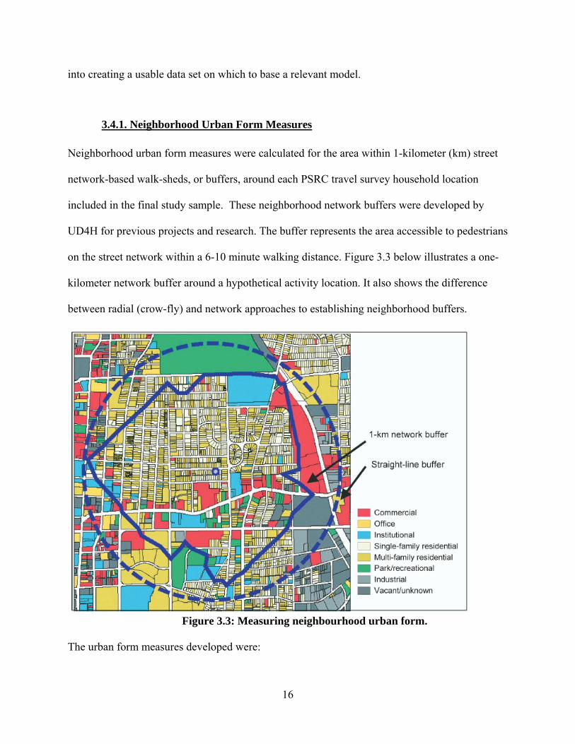


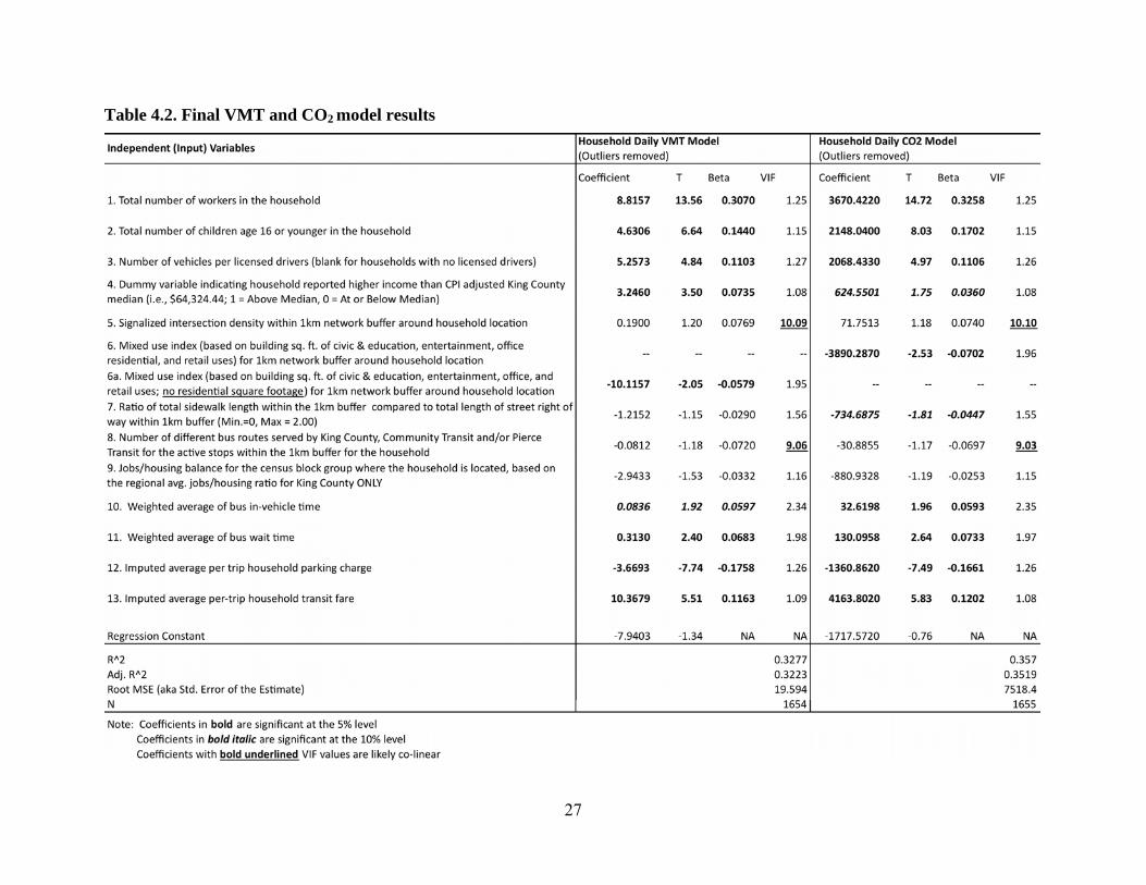


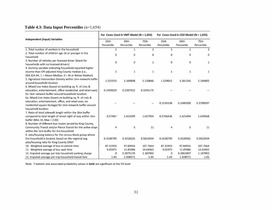


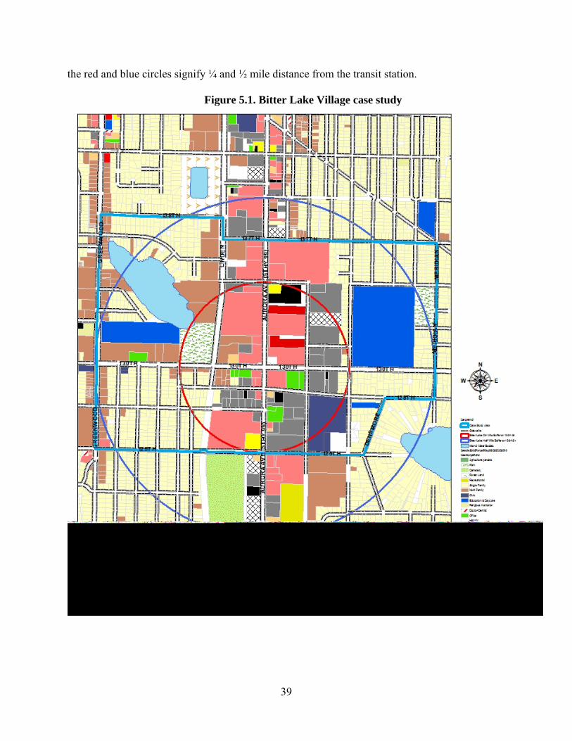


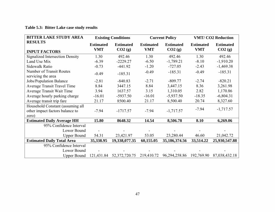


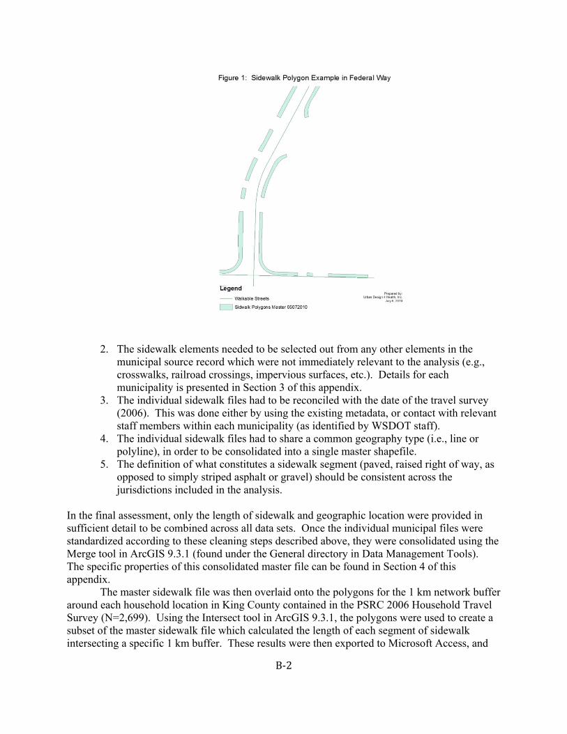


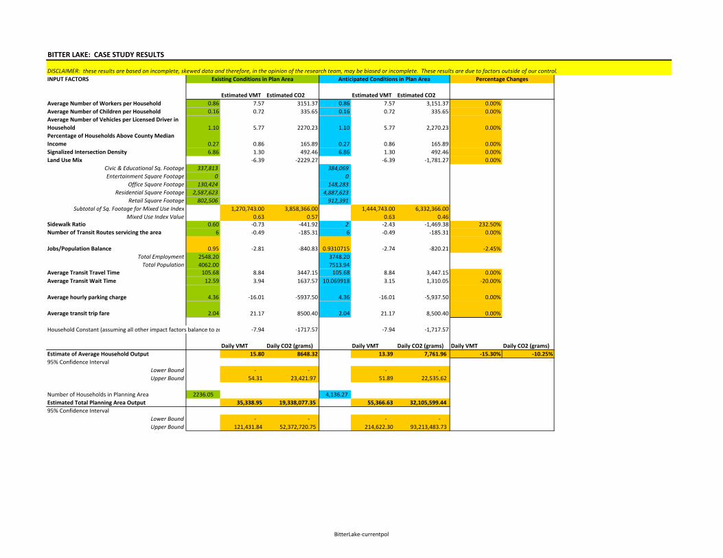


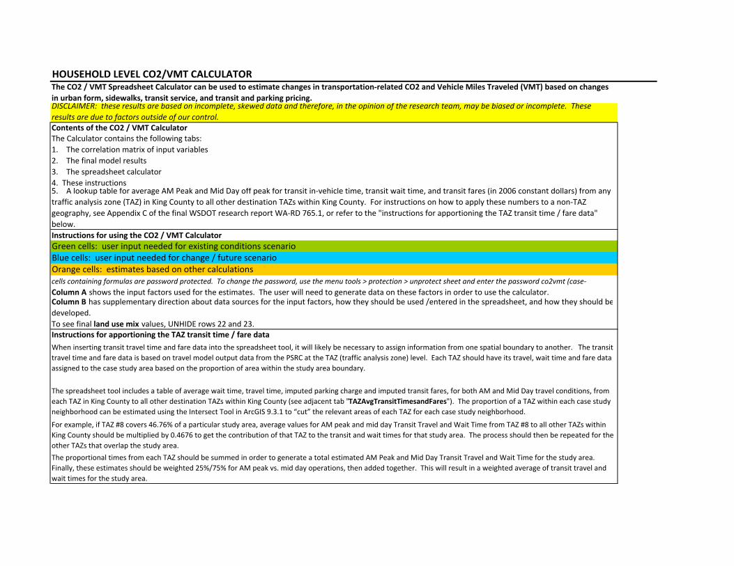

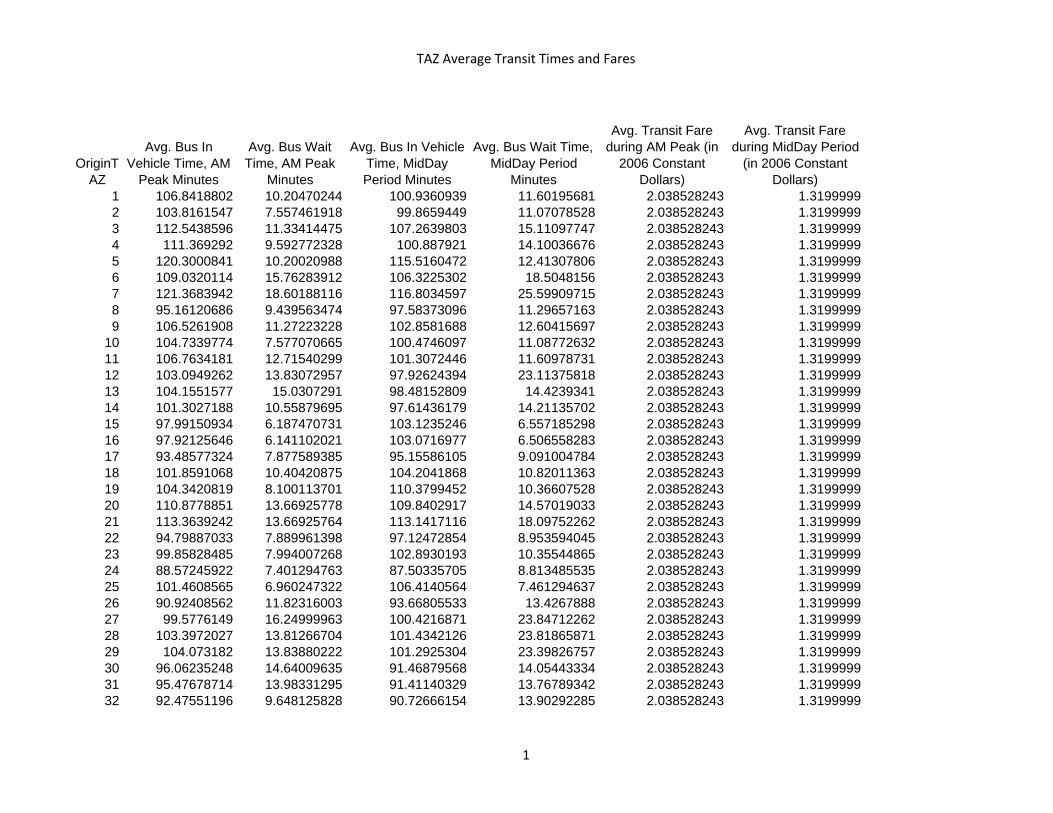


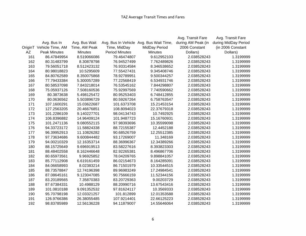


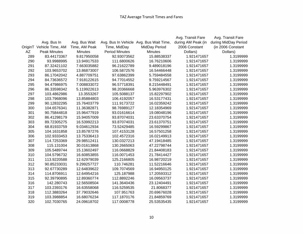


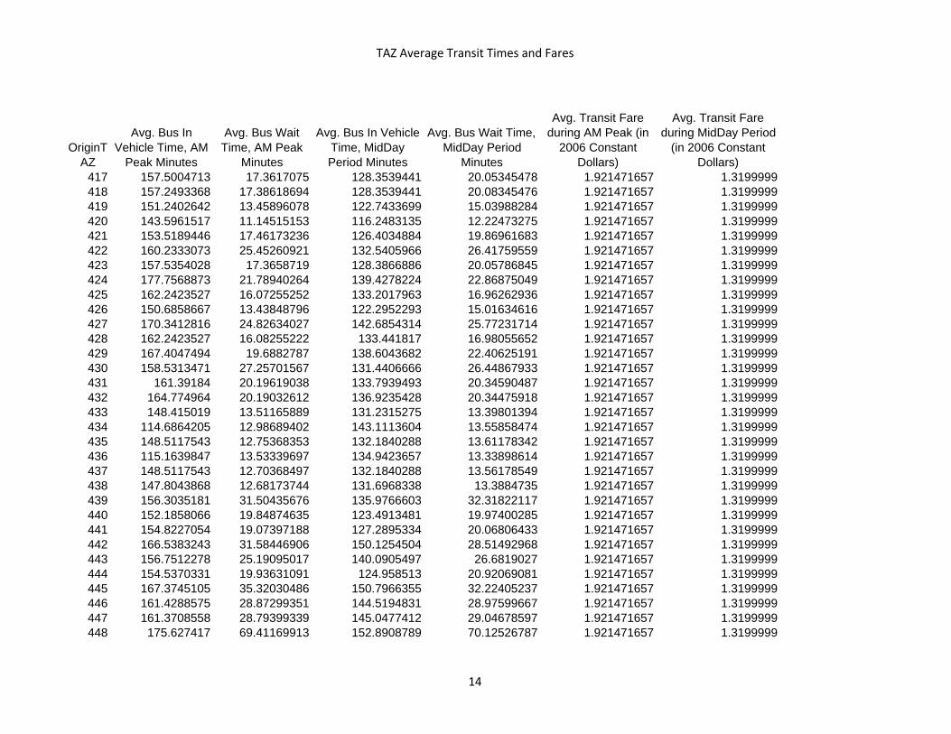
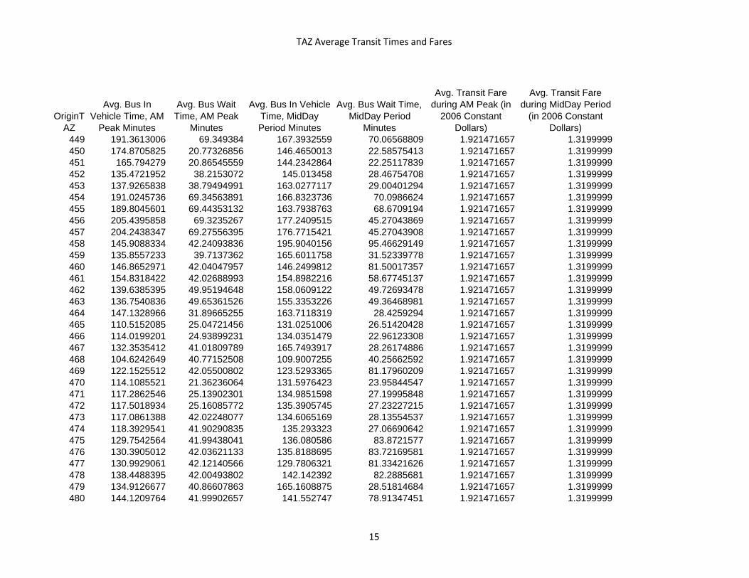


![3. DUMMY VARIABLES, NONLINEAR VARIABLES AND SPECIFICATIONminiahn/ecn725/cn3_dummy.pdf · 2006-03-07 · DUMMY VARIABLES, NONLINEAR VARIABLES AND SPECIFICATION [1] DUMMY VARIABLES](https://static.documents.pub/doc/80x56/5b90b6d509d3f21c788c95bb/3-dummy-variables-nonlinear-variables-and-miniahnecn725cn3dummypdf-2006-03-07.jpg)


