1

AN ASYMPTOTIC FORMULATION FOR THE INFUSION OF A THERAPEUTIC AGENT

INTO A SOLID TUMOR MODELED AS A POROELASTIC MEDIUM

Alessandro Bottaro and Tobias Ansaldi

DICAT - Centro di Ricerca in Tecnologie dei Materiali

Università di Genova

1, via Montallegro, 16145 Genova, Italy

Corresponding author: Alessandro Bottaro

Department of Civil, Environmental and Architectural Engineering

Centro di Ricerca in Tecnologie dei Materiali

Engineering Faculty, University of Genova

1, via Montallegro

16145 Genova, Italy

Tel. +39 – 010 – 3532540

Fax. +39 – 010 – 3532546

Email: alessandro.bottaro@unige.it

Keywords: Solid tumor, Infusion, Poroelasticity, Asymptotic model, Fluid mechanics

Word count: Abstract: 164 words

Approximate word count for the text: 3000 words

(plus 1 table and 7 figures)

2

AN ASYMPTOTIC FORMULATION FOR THE INFUSION OF A THERAPEUTIC AGENT

INTO A SOLID TUMOR MODELED AS A POROELASTIC MEDIUM

Alessandro Bottaro and Tobias Ansaldi

DICAT – Centro di Ricerca in Tecnologie dei Materiali

Università di Genova

1, via Montallegro, 16145 Genova, Italy

Abstract

The direct infusion of an agent into a solid tumor, modeled as a spherical poroelastic material with

anisotropic dependence of the tumor hydraulic conductivity upon the tissue deformation, is

treated both by solving the coupled fluid/elastic equations, and by expressing the solution as an

asymptotic expansion in terms of a small parameter, ratio between the driving pressure force in

the fluid system and the elastic properties of the solid. Results at order one match almost

perfectly the solutions of the full system over a large range of infusion pressures. A comparison

with experimental results by McGuire et al. (2006) provides acceptable agreement after the

hydraulic conductivity of the medium is properly calibrated. Given the wide range of variation of

some model constants, the order zero solution of the expansion – for which fluid and porous

matrix are decoupled – yields acceptable values and trends for all the physical fields of interest.

When the deformation of the tissue becomes large nonlinear elasticity theory must be resorted to.

1. Introduction

In recent years it has become common to shrink solid tumors before surgery via intratumoral

injection of chemotherapeutic drugs, to allow cleaner/simpler/less destructive removal, or to

render operable possibly inoperable tumors. Efficient delivery of a therapeutic agent within a

solid tumor via intratumoral infusion requires a thorough understanding of the fluid dynamics in

the gel-like region between cells (the interstitium). A number of physiological barriers opposes the

infusion: the abnormally elevated density of cancer cells limits drug transport by constricting

intratumoral blood vessels; the high interstitial fluid pressure (IFP) which occurs within the tumor

and the lack of functional lymphatics hamper convective transport of the agents to the

interstitium; and the tumor microvasculature is leaky. The main obstacle to efficient delivery is

believed to be the high IFP (values up to 50 mmHg have been reported in solid tumors, Baxter and

Jain 1989; Boucher et al. 1991; Roh et al. 1991; Gutmann et al. 1992); it can produce some

reabsorption of fluid by the capillary network with the consequence that not all the therapeutic

agent injected diffuses within the tumor tissues.

It is common to model the problem of the transport of drugs and nutrients within a solid tumor by

considering it as a fluid-saturated porous medium, characterized by the hydraulic conductivity K of

the tissue (ratio between the permeability of the medium and the dynamic viscosity of the fluid)

and by its Lamé coefficients, G and . Assuming negligible lymphatic drainage, the parameters

needed to describe transvascular fluid exchange – within the Starling’s law assumption – are the

3

hydraulic conductivity of the capillary walls Lp, the vascular surface area per unit volume S/V and

the effective vascular pressure pe. Macroscopic parameters can in principle be inferred from

homogenizing the microscopic features of the tumor, i.e. its morphology as a micro-structured

material, with fiber matrix, proteins, fluid in the interstitial matrix, and including the fluid

exchange with the capillaries embedded in the interstitium (see Shipley and Chapman (2010) for

recent progress on this). A more common approach is to infer values of the governing parameters

from in vivo and in vitro measurements. Smith and Humphrey (2007) provide a review of

measured values from the literature.

The rate of fluid flow within the tumor depends on the value of K of the tissues which can, in turn,

be strongly altered by the deformation of the tissues themselves. It has been found (Zhang et al.

2000) that variations of the hydraulic conductivity by several orders of magnitude may take place

with a four-fold increase of the infusion pressure, as a result of tissue expansion and compression.

The coupling between the deformation of the tumor and its conductivity is hence crucial, and the

use of poroelasticity theory has been proposed, see for example Netti et al. (1995) or

Sarntinoranont et al. (2003). Whereas various empirical relations for K = K(u), with u the

displacement of the solid, are present in the literature (ex. Lai and Mow 1980; Barry and Aldis

1990), only McGuire et al. (2006) consider a non-linear, anisotropic relation.

In this work we follow the lead of McGuire et al. (2006) to study the intratumoral infusion of a

therapeutic agent into an isolated solid tumor of spherical shape, i.e. a tumor that is not

surrounded by normal tissue. A perturbation approach is proposed within the linear elastic

approximation, with the solution expressed in term of powers of a small dimensionless parameter

, defined as the ratio between an effective pressure at the infusion site and the tissue solid

properties (expressed via a linear combination of G and ). Comparison between results obtained

with the full model and with the perturbation analysis (up to order ) provide an indication on the

range of applicability of the asymptotic approach.

2. The model

Tumors are strongly heterogeneous and are often modeled as being formed by concentric layers

of tissue (eventually including a necrotic core) of thickness defined by the proliferation/quiescent

activity of the cancer cells; here, we consider a spherical tumor of radius R, whose sources of

radial inhomogeneity are in the hydraulic conductivity of the tumor interstitium K and in the

hydraulic conductivity of the capillary walls Lp. A drug is infused at the center by a needle,

creating a small fluid cavity around the tip of radius a (cf. fig. 1). As fluid is injected, the cavity

deforms mildly and, at the steady state, the fluid fills a spherical cavity of radius a’. Likewise, the

radius of the tumor becomes R’ in steady infusion conditions. Spherical symmetry is maintained

and the radial component rr of the stress tensor T, in the linear elastic approximation, is

rr = - p + (2G + ) ur + 2 u/r (1)

4

with p the IFP, u the radial displacement of the solid, and r the radial coordinate (when r is used as

subscript a derivation is intended, except when the subscript denotes the component of a tensor,

ex. rr orrr). The term [(2G + ) ur + 2 u/r] is the radial contact stress. By setting to zero the

divergence of T it is obtained:

(2G )(ur + 2u/r)r = pr (2)

The conservation of mass in the fluid phase within the Darcy flow assumption is:

– (r2 K pr)r/r2 = Lp (pe – p) S/V (3)

with the right-hand-side, the Starling’s law term, which can act as either a source or a sink because

of the leakiness of the tumor microvasculature. Since the tumor vasculature is structurally and

functionally abnormal, it is common to assume a constant value of pe; conversely, to account for

the heterogeneous distribution of capillaries, and in particular for the increased activity of cancer

cells towards the outer boundary of the tumor, where they coopt host vessels to obtain nutrients

for their growth and sprout new vessels from existing ones, we assume Lp to vary with r as:

Lp = Lp0 f(r/R), (4)

with f(r/R) a dimensionless function ranging from zero to one

To model anisotropic effects in the hydraulic conductivity K we assume, following McGuire et al.,

that

K = K0 exp{M[rr + (1 – ) (+ )/2} (5)

with K0, M, model constants,rr , and components of the strain tensor defined byrr = ur

and = = u/r. The equations are closed by boundary conditions, i.e.

p(R’) = 0; p(a’) = pinfusion; (2G ) ur(R’) + 2 u(R’)/R’ = 0; .

– p(a’) + (2G ) ur(a’) + 2 u(a’)/a’ = – pinfusion. (6)

The latter two relations specify, respectively, the absence of radial contact stresses at the tumor

margins r = R’, and the continuity of the radial components of the stress across the interface in

r = a’ between the cavity and the porous matrix (Truskey et al. 2009). Since a’ and R’ are a priori

unknown, the boundary conditions in the full model are enforced at a and R, under the hypothesis

of small deformations.

Normalization of equations and boundary conditions brings out the relevant parameters of this

model. We thus scale the IFP with (pinfusion – pe), the displacement u and the radial coordinate r

with R, and the hydraulic conductivity K with K0, isolating two dimensionless parameters:

= (pinfusion – pe)/(2G ) (7)

2 = (Lp0/K0) R2 S/V (8)

5

The first parameter characterizes the ratio between the driving pressure forces in the fluid system

and the elastic properties of the solid; the second parameter measures the relative importance of

the resistance to interstitial percolation with respect to the resistance to transcapillary fluid

exchange (Baxter and Jain 1989, 1990). Typically is much smaller than one, whereas is of order

one.

The equations in terms of dimensionless variables read:

(ur + 2u/r)r = pr (9)

(r2 K pr)r = r2 2 (p – pe) f(r) (10)

K = exp{M[ur + (1 – ) u/r]} (11)

with boundary conditions:

p(1) = 0; p(a) = pinfusion; ur(1) + 2 2G ) u(1) = 0; ur(a) + 2 2G ) u(a)/a = (12)

and anow scaled by R. Equations (9-12) are solved by a finite difference second order iterative

scheme, yielding solutions for p, the hydraulic conductivity K, the Darcy flux q = – K pr and the flow

rate Q of the therapeutic agent through the tumor, for parameters corresponding to some of the

measurements by McGuire et al. We denote with Qinfusion the value of Q at r = a.

3. The perturbation approach

A second approach to the solution of the problem begins by expanding the dependent variables

into regular power series of (Bonfiglio et al. 2010) as:

u = u1 + O(2),

p = p0 + p1 + O(2),

K = 1 + K1 + O(2),

with K1 = M[ u1r + (1 - ) u1/r]. Upon inserting into equation (10) the equation at order 0 is:

(r2 p0r)r = r2 2 (p0 – pe) f(r), (13)

with boundary conditions p0(1) = 0 and p0(a) = pinfusion. The solution in the Lp = Lp0 limit is simply:

p0 = pe + A er/r + B e-r/r (14)

with A and B easily available from the boundary conditions. For f(r) not uniformly equal to one,

the zeroth order pressure field can be found by numerical integration of eq. (13). From p0 it is

then easy to recover the leading order Darcy flux q0 and flow rate Q0. At order the equations

are:

6

(u1r + 2u1/r)r = p0r (15)

(r2 K0 p1r + r2 K1 p0r)r = r2 2 p1 f(r), (16)

together with

p1(1) = – u1(1) p0r(1)

p1(a) = – u1(a) p0r(a)

u1r (1) + 2 2G ) u1(1) = 0

u1r(a) + 2 2G ) u1(a)/a = 0 (17)

obtained by Taylor expanding the boundary conditions in eq. (6) around r = a and r = R, and

collecting terms of order . The variables p1, K1 and u1, as well as q1 and the infusion flow rate at

order , can be obtained by a central difference numerical method, similar to that used for eqs. (9-

12). In both cases we have employed a large number of uniformly distributed radial grid points

(up to 6000) to ensure that all results presented are grid-converged.

4. Results

The configuration examined here correspond to the 4T1 cell lines used in the study by McGuire et

al. These lines had the highest collagen concentration among the tested ones, and showed a

strongly non-linear relation between the infusion pressure and the infusion rate. They were

murine mammary carcinoma cell lines, injected subcutaneously into mice. After the tumor had

grown to a diameter of the order of the centimeter, a solution was infused into the center of the

tumor with a needle, until a small fluid cavity approximately equal to the needle radius was

formed. From that point on, increasing and measuring the infusion pressure, McGuire et al. could

measure the corresponding flow rate of the solution entering the tissue. Errors on the measured

pressures could be quantified to be less than 3.7 mmHg. In table 1 a list of all parameters

employed in the present simulations is given.

Physical variable or model constant

Definition Corresponding dimensionless value

a = 0.18 mm Unperturbed radius of the inner cavity

a = 0.036

R = 0.5 cm Unperturbed radius of the tumor

R = 1

K0 = 3 x 10-5 cm2/(mmHg s) (smaller values are typically given in the literature, e.g. Smith and Humphrey 2007)

Model constant in eq. (5)

7

M = 10 Model constant in eq. (5)

0 < < 1; = 0.733 was the best fit with the data for the model by McGuire et al.

Model constant in eq. (5)

Pe = 11.25 mmHg Effective vascular pressure (Smith and Humphrey 2007)

30 mmHg ≤ pinfusion ≤ 70 mmHg Infusion pressure 1.6 ≥ pinfusion ≥ 1.1915

Lp0 = 1.3332 x 10-6 cm/(mmHg s) Vascular conductivity at r = R

(Smith and Humphrey 2007)

S/V = 200 cm2/cm3 Vascular surface area per unit volume (Smith and Humphrey 2007)

2 = 2.2222 (eq. 6)

10 mmHg ≤≤ 1000 mmHg

= 175 mmHg was the best fit with the data for the model by McGuire et al.

Lamé coefficient

G = 75 mmHg (corresponding

to = 175 mmHg once the

Poisson ratio is fixed at 0.35)

Shear modulus

0.05769 ≤ ≤ 0.1807 Small parameter in the expansion (eq. 7)

Table 1: List of relevant dimensional and dimensionless parameter. All of them

have been taken from McGuire et al. except where otherwise indicated.

Three cases are considered next, denoted as cases 1, 2 and 3. The first assumes a constant value

of Lp = Lp0, i.e. f(r) = 1. In the second case it is assumed that f(r) increases radially outwards as

f(r) = exp[b(r – 1)/(1 – a)], with b = log(10); the value of Lp at r = R is equal to Lp0 and it is ten times

larger than the corresponding value at r = a. The factor of ten is arbitrary, but within the range of

values reported in the literature (Baxter and Jain 1989; Smith and Humphrey 1997). In the third

case we make the hypothesis that transvascular fluid exchange is concentrated near the tumor

outer margins, possibly as a result of strong localized angiogenesis, so that f(r) = exp[ – 150 (r – 1)2].

These three distributions cover a large spectrum of configurations, and are plotted in fig. 2. In figs.

3 and 4 results are reported from simulations using the full model, i.e. eqs. (9-12), at = 0.05

(corresponding to pinfusion = 27.5 mmHg) and = 0.2 (pinfusion = 76.25 mmHg). As expected the

deformation u is larger for larger infusion pressure. The trend of the u-curves with r varies with

the case considered: it decreases rapidly near the infusion site for all cases, to eventually increase

(case 1), settle (case 2) or slowly decrease (case 3). Perhaps unexpectedly the conductivity K of

the tissue is but mildly affected by variations in the hydraulic conductivity of the capillary walls; in

both fig. 3 and 4 one observes a very steep increase of K from the infusion point, and a rapid

equilibration around K ≈ 1. The IFP decreases monotonically in r from pinfusion to zero, with little

effect of Lp, while the flow rate increases. This is related to extravasation of fluid from the vessels

into the tumor interstitium, not balanced by resorption into lymphatics.

8

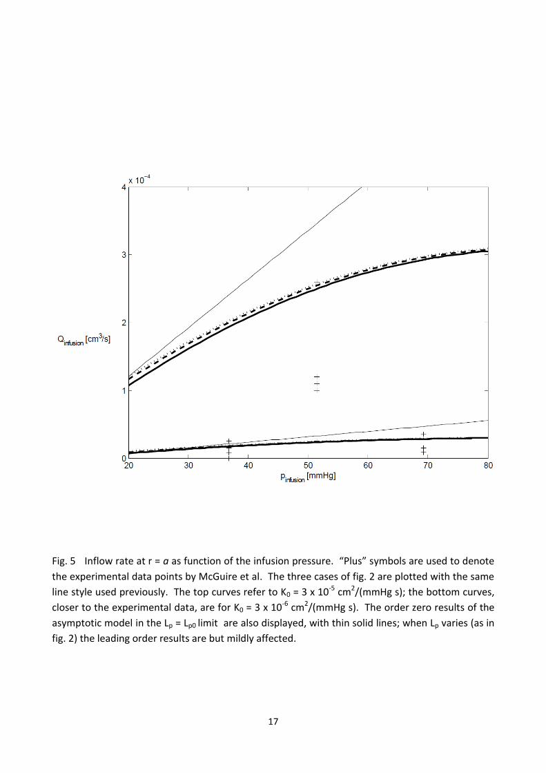
Denoting by Qinfusion the rate of agent entering the tumor at r = a, the (now dimensional) variation

of Qinfusion with pinfusion is displayed in fig. 5, for the three cases of fig. 2. It is interesting to observe

that for the value of K0 employed by McGuire et al. – which is the average value measured in their

experiments – our model overestimates the infusion rate. On the other hand, values of the

average hydraulic conductivity typically lower than 3 x 10-5 cm2/(mmHg s) are often reported for

neoplastic tissues (see e.g. Smith and Humphrey (2007) who report a range between 4 x 10-9

cm2/(mmHg s) and 2.5 x 10-6 cm2/(mmHg s)). In fig. 5 we have therefore also included results for

the three cases of figure 2 for a value of K0 ten times smaller than indicated by McGuire et al.,

obtaining a better match with experimental data. McGuire et al. observed a marked reduction of

the infusion rate after the infusion pressure exceeds 50 mmHg (cf. fig. 4, bottom frame, of

McGuire et al.) and argued that the bell-shaped curve in the pinfusion-Qinfusion plane is partly related

to the formation of a thin membrane around the needle tip, forcing the pressure at r = a to be

above a given threshold before intratumoral infusion can take place. The existence of a threshold

pressure for infusion had been observed previously (McGuire and Yuan 2001) and the mechanism

still awaits a complete physical description. Another possible reason of discrepancy between the

numerical results that we have obtained and those by McGuire et al. is due to the neglect/account

of fluid exchange between the interstitium and the blood vessels. Accounting for it, via the

Starling’s law term, we find that Q increases with r with fluid filling the extra-cellular matrix and

contributing to the increase of the strain. Fig. 5 shows also results obtained from the asymptotic

model at order zero, with constant Lp = Lp0 (i.e. results directly available from eq. 14). It is

interesting to observe that – particularly at low infusion pressures – they do not differ much from

the solutions of the full system (9-12), and are similarly affected by variations in K0. As expected,

the agreement between the exact solution of the full model and the leading order solution

deteriorates with the increase of . Given the uncertainties in the estimate of the hydraulic

conductivity, for practical purposes, in the limit of very small deformations, it seems that the

leading order term of the expansion yields field values which are sufficiently accurate. On the

other hand, for “large” deformations (within the limits of linear elasticity theory), it is appropriate

to extend the asymptotic solution up to next higher order.

The accuracy of the expansion proposed can be inferred from inspection of figs. 6 and 7. Here the

solutions, up to order of the asymptotic model are drawn together with the results of the full

system of equations (9-12), for two cases, = 0.1 and 0.3, corresponding, respectively, to pinfusion =

43.75 mmHg and pinfusion = 108.75 mmHg. Case 1 has been treated in both figures. The agreement

is generally good, despite the fact that the larger value of pinfusion exceeds by much those

commonly encountered in applications; such a large value of is of interest only to test the

limitations of the asymptotic analysis. The validity of the latter statement stems also from Jain’s

(1987) observation that the porosity of the interstitial matrix is approximately 0.2; this means

that the pore velocity (equal to the Darcy flux q divided by ) can be properly represented by the

expansion proposed only when is much smaller than 0.2. In the results shown here we have

fixed K0 to the value of 3 x 10-6 cm2/(mmHg s) which appears to provide flow rates of the agent at

r = a closer to the measured ones. The plots of the IFP resemble those presented by Smith and

Humphrey (2007) for a similar configuration. The pressure decays over a small radial distance

9

from the infusion site, it remains close to the effective vascular pressure over a range of r, before

ultimately decaying to the value imposed at the tumor margin. When the infusion pressure is very

large ( = 0.3) the agreement between the asymptotic solution at order and the full solution

deteriorates, particularly as far as u is concerned, yielding a negative value of the hydraulic

conductivity very close to the infusion site; whereas one could go to second order to improve

matters, this is not consistent with linear elasticity theory which holds to first order in the

deformation.

5. Closing remarks

An asymptotic approach has been proposed for the study of the infusion of a therapeutic agent

into a solid tumor, modeled as a poroelastic medium of conductivity anisotropically dependent on

the material strain rate. In the model we have included fluid exchange with the capillary, and

observed the minor influence of variations of the vascular conductivity Lp on the results. The

parameter which influences the most the results is the average hydraulic conductivity K0 of the

medium, whereas the radial distribution of K holds a relatively minor role. Given the large scatter

of data present in the literature for K0, there seems to be little need in coupling the elastic

deformation of the fluid with the hydraulic properties of the interstitium: the leading order,

uncoupled, solution is sufficiently accurate, at least for sufficiently low values of the infusion

pressure. The situation is obviously different should large strains of the tissue occur.

Several lines of research arise in light of the results reported here. One is based on the use of

nonlinear theory for the behavior of materials undergoing strong displacements; the neo-Hookean

material, often used for modeling elastin and collagen, could possibly be used, as well as the Fung-

elastic constitutive model (Fung 1993, Sun and Sacks 2005), appropriate for soft tissues

characterized by pronounced mechanical anisotropy, highly nonlinear stress–strain relationships,

large deformations, and viscoelasticity. Another avenue of research consists in developing a

model which couples the intravascular and interstitial flow, reducing the need for model constants

of uncertain determination. Progress along this line has been recently reported by Wu et al.

(2008, 2009). Finally, even assuming that the tumor has a spheroidal shape, given the haphazard

formation of cracks, hypoxic and necrotic regions in tissues it is estimated that only about 20% of

the cases end up with a spherical distribution of flow and drugs (personal communication of Prof.

Fan Yuan), with irregular, three-dimensional infusion in all other cases. This is one of the major

problems to overcome when modeling intratumoral infusion.

Conflict of interest statement

The authors declare to have no financial or personal relationships with other people or

organizations that could inappropriately influence their work.

10

Acknowledgements

We gratefully acknowledge the insightful comments by Prof. Fan Yuan, Dr. Rodolfo Repetto and

Dr. Marina Artuso.

References

Barry, S.I., Aldis, G.K., 1990. Comparison of models for flow induced deformation of soft biological

tissues. J. Biomech. 23, 647-654

Baxter, L.T., Jain, R.K., 1989. Transport of fluid and macromolecules in tumors. I. Role of interstitial

pressure and convection. Microvasc. Res. 37, 77-104

Baxter, L.T., Jain, R.K., 1990. Transport of fluid and macromolecules in tumors. II. Role of

heterogeneous perfusion and lymphatics. Microvasc. Res. 40, 246-263

Bonfiglio, A., Leungchavaphongse, K., Repetto, R., Siggers, J. H., 2010. Mathematical modeling of

the circulation in the liver lobule. J. Biomech. Eng (ASME), 132, 111011

Boucher, Y., J., Kirkwood, M., Opacic, D., Desantis, M., Jain, R.K., 1991. Interstitial hypertension in superficial metastatic melanomas in patients. Cancer Res. 51, 6691–6694 Fung, Y.C., 1993. Biomechanics. Mechanical Properties of Living Tissues. Springer Gutmann, R., Leunig, M., Feyh, J., Goetz, A.E., Messmer, K., Kastenbauer, E., Jain, R.K., 1992. Interstitial hypertension in head and neck tumors in patients: Correlation with tumor size. Cancer Res. 52, 1993–1995 Jain, R.K., 1987. Transport of molecules in the tumor interstitium: a review. Cancer Res. 47, 3039-3051

Lai, W.M., Mow, V.C., 1980. Drag-induced compression of articular cartilage during a permeation

experiment. Biorheology 17, 111-123

McGuire, S., Yuan, F., 2001. Quantitative analysis of intratumoral infusion of color molecules. Am.

J. Physiol. 281, H715-H721

McGuire, S., Zaharoff, D., Yuan, F., 2006. Nonlinear dependence of hydraulic conductivity on tissue

deformation during intratumoral infusion. Annals Biomed. Eng. 34, 1173-1181

Netti, P.A., Baxter, L.T., Boucher, Y., Skalak, R.K., Jain, R.K., 1995. A poroelastic model for

interstitial pressure in tumors. Biorheology 32, 346

Roh, H. D., Boucher, Y., Kalnicki, S., Buchsbaum, R., Bloomer, W.D., Jain, R.K., 1991. Interstitial hypertension in carcinoma of uterine cervix in patients: Possible correlation with tumor oxygenation and radiation response. Cancer Res. 51, 6695–6698

11

Sarntinoranont M., Rooney, F., Ferrari, M., 2003. Interstitial stress and fluid pressure within a

growing tumor. Annals Biomed. Eng. 31, 327-335

Shipley, R.J., and Chapman, S.J., 2010. Multiscale modelling of fluid and drug transport in vascular

tumours. Bull. Math. Biology 72, 1464-1491

Smith, J.H., Humphrey, J.A.C., 2007. Interstitial transport and transvascular fluid exchange during

infusion into brain and tumor tissue. Microvascular Res. 73, 58-73

Sun, W., Sacks, M.S., 2005. Finite element implementation of a generalized Fung-elastic

constitutive model for planar soft tissues. Biomechan. Model Mechanobiol. 4, 190–199

Truskey, G.A., Yuan, F., Katz, D.F., 2009 Transport phenomena in biological systems. Pearson

Prentice Hall Bioengineering, second edition

Wu, J., Long, Q., Xu, S., Padhani, A.R., 2009 Study of tumor blood perfusion and its variation due to

vascular normalization by anti-angiogenic therapy based on 3D angiogenic microvasculature. J.

Biomech. 42, 712-721

Wu, J., Xu, S., Long, Q., Collins, M.W., König C.S., Zhao, G., Jiang Y., Padhani A.R., 2008. Coupled

modeling of blood perfusion in intravascular, interstitial spaces in tumor microvasculature. J.

Biomech. 41, 996-1004

Zhang, X.-Y., Luck, J., Dewhirst, W.M., Yuan, F., 2000. Interstitial hydraulic conductivity in a

fibrosarcoma. Am. J. Physiol. 279, H2726-H2734

12

Figure captions

Fig. 1. Section of a solid tumor of spherical shape. The magnified view on the right shows a detail

of the porous interstitium, with the micro-vasculature created around the tumor cells.

Fig. 2. Radial distribution of the hydraulic conductivity coefficient of the capillary walls Lp for cases

1 to 3, as reported in the text.

Fig. 3 Solution of the full model for = 0.05. From top left frame, and clockwise: radial

distribution of the displacement u, of the hydraulic conductivity K of the tissue, of the flow rate Q

through any given spherical surface at radius r (including transvascular fluid exchange), and of the

IFP. Cases 1 to 3 with line styles as in fig. 2. The thin horizontal line in the figure with the IFP

denotes the dimensionless value of the effective vascular pressure.

Fig. 4 Solution of the full model for = 0.2. From top left frame, and clockwise: radial distribution

of the displacement u, of the hydraulic conductivity K of the tissue, of the flow rate Q through any

given spherical surface at radius r (including transvascular fluid exchange), and of the IFP. Cases 1

to 3 with line styles as in fig. 2. The thin horizontal line in the figure with the IFP denotes the

dimensionless value of the effective vascular pressure.

Fig. 5 Inflow rate at r = a as function of the infusion pressure. Symbols are used to denote the

experimental data points by McGuire et al. The three cases of fig. 2 are plotted with the same line

style used previously. The top curves refer to K0 = 3 x 10-5 cm2/(mmHg s); the bottom curves,

closer to the experimental data, are for K0 = 3 x 10-6 cm2/(mmHg s). The order zero results of the

asymptotic model in the Lp = Lp0 limit are also displayed, with thin solid lines; when Lp varies (as in

fig. 2) the leading order results are but mildly affected.

Fig. 6 Exact (thick solid lines), order zero (this solid lines) and order one asymptotic results

(dashed lines) for pinfusion = 43.75 mmHg ( = 0.1) and K0 = 3 x 10-6 cm2/(mmHg s). The leading

order value of u is zero and K0 = 1 (not drawn). The horizontal line in the frame with the IFP

denotes the effective vascular pressure.

Fig. 7 Exact (thick solid lines), order zero (this solid lines) and order one asymptotic results

(dashed lines) for pinfusion = 108.75 mmHg ( = 0.3) and K0 = 3 x 10-6 cm2/(mmHg s). The horizontal

line in the frame with the IFP denotes the effective vascular pressure.

13

Fig. 1. Section of a solid tumor of spherical shape, with inner cavity filled with fluid. The

magnified view on the right shows a detail of the porous interstitium, with the micro-vasculature

created around the tumor cells.

14

Fig. 2. Radial distribution of the hydraulic conductivity coefficient of the capillary walls Lp for cases

1 to 3, as reported in the text. Case 1: solid line; case 2: dashed line; case 3: dotted line.

15

Fig. 3 Solution of the full model for = 0.05. From top left frame, and clockwise: radial

distribution of the displacement u, of the hydraulic conductivity K of the tissue, of the flow rate Q

through any given spherical surface at radius r (including transvascular fluid exchange), and of the

IFP. Cases 1 to 3 with line styles as in fig. 2. The thin horizontal line in the figure with the IFP

denotes the dimensionless value of the effective vascular pressure.

16

Fig. 4 Solution of the full model for = 0.2. From top left frame, and clockwise: radial distribution

of the displacement u, of the hydraulic conductivity K of the tissue, of the flow rate Q through any

given spherical surface at radius r (including transvascular fluid exchange), and of the IFP. Cases 1

to 3 with line styles as in fig. 2. The thin horizontal line in the figure with the IFP denotes the

dimensionless value of the effective vascular pressure.

17

Fig. 5 Inflow rate at r = a as function of the infusion pressure. “Plus” symbols are used to denote

the experimental data points by McGuire et al. The three cases of fig. 2 are plotted with the same

line style used previously. The top curves refer to K0 = 3 x 10-5 cm2/(mmHg s); the bottom curves,

closer to the experimental data, are for K0 = 3 x 10-6 cm2/(mmHg s). The order zero results of the

asymptotic model in the Lp = Lp0 limit are also displayed, with thin solid lines; when Lp varies (as in

fig. 2) the leading order results are but mildly affected.

18

Fig. 6 Exact (thick solid lines), order zero (thin solid lines) and order one asymptotic results

(dashed lines) for pinfusion = 43.75 mmHg ( = 0.1) and K0 = 3 x 10-6 cm2/(mmHg s). The leading

order value of u is zero and K0 = 1 (not drawn). The horizontal line in the frame with the IFP

denotes the effective vascular pressure.

19

Fig. 7 Exact (thick solid lines), order zero (thin solid lines) and order one asymptotic results

(dashed lines) for pinfusion = 108.75 mmHg ( = 0.3) and K0 = 3 x 10-6 cm2/(mmHg s). The horizontal

line in the frame with the IFP denotes the effective vascular pressure.