Page 1
AN ATTAINABLE REGION APPROACH TO
OPTIMIZING PRODUCT SIZE DISTRIBUTION FOR
FLOTATION PURPOSES
Ngonidzashe Chimwani
A thesis submitted to the Faculty of Engineering and the Built Environment,
University of the Witwatersrand, Johannesburg, in fulfilment of the requirements
for the degree of Doctor of Philosophy in Engineering
Johannesburg, 2014
Page 2
ii
Declaration
I declare that this thesis is my own unaided work. It is being submitted for the
degree of Doctor of Philosophy in Engineering in the University of the
Witwatersrand, Johannesburg. It has never been submitted either in part or in
whole for a degree in this or any other University.
...........................................................
Ngonidzashe Chimwani
..............day of...........................year..............
Page 3
iii
Abstract
In this thesis, experimental and modelling techniques were used to investigate the
breakage of a typical South African platinum group minerals ore in a ball mill to
optimize product size distribution (PSD) for flotation purposes.
Batch milling experiments were conducted on three narrow-sized feeds using
three different ball sizes to determine the milling parameters of the platinum ore.
Verification of the parameters was done by doing additional tests beyond the
previous experimental range. This confirmed that the parameters were good
estimates for the ore. A scale-up procedure for batch grinding data was used to
obtain parameters for an industrial mill on which a performance survey had been
done. The survey data was used to verify the scale-up parameters. Following this,
the effects of mill rotational speed, ball filling level, slurry filling and ball sizes on
milling kinetics were explored and analysed using the attainable region (AR)
technique.
The outcomes of the simulations showed that a finer product is achieved when
small balls are used. Lower mill hold-up and fewer grinding balls were also
shown to enhance finer grinding. However, factors that produced a coarser
product as shown by the particle size analysis were shown to yield the greatest
amount of the desired size class when analysed using AR.
Next, the AR technique was used to analyse simulation outputs of a continuous
mill over a wide range of operating conditions. The analysis was limited to plug-
flow and well-mixed mill transport models without exit classification. The AR
analysis showed that industrial milling conditions could be tailored to the desired
product by reducing residence time, mill speed while increasing ball size.
Extension of the AR framework to a more realistic transport model also produced
similar results. The importance of optimally controlling the residence time of
material inside a mill as well as energy was demonstrated when maximising the
desired size range. The results showed that operating the ball mill at lower speeds
and higher ball filling saves energy.
Page 4
iv
Finally, combining the population balance modelling technique and the AR
enabled a better understanding and effective optimisation of milling for
downstream processes, particularly for flotation.
Page 5
v
Publications
The papers published by the author on the contents of this thesis are as follows:
Chimwani, N., Glasser, D., Hildebrandt, D., Metzger, M.J., Mulenga, F.K., 2013.
Determination of the milling parameters of a platinum group minerals ore to
optimize product size distribution for flotation purposes. Minerals Engineering,
vol. 43 – 44, pp. 67 – 78
Chimwani, N., Mulenga, F.K.., Glasser, D., Hildebrandt, D., Bwalya, M., 2014.
Scale-up of batch grinding data for simulation of industrial milling of platinum
group minerals ore. Minerals Engineering, in press
Mulenga, F.K., Chimwani, N., 2013. Introduction to the use of the attainable
region method in determining the optimal residence time of a ball mill.
International Journal of Mineral Processing, vol. 125, pp. 39 – 50
Chimwani, N., Mulenga, F.K.., Glasser, D., Hildebrandt, D., Bwalya, M., 2014.
Use of the attainable region method to simulate a full-scale ball mill with a
realistic transport model, presented at the Comminution 14’ in Cape Town,
Minerals Engineering International Conference
Page 6
vi
Dedications
This work is dedicated to all my
family members
Page 7
vii
Acknowledgements
Firstly, I would like to exalt the Almighty GOD, the author of my life, who
allowed me to do a PhD thesis. My LORD, thank you for giving me wisdom,
proper guidance and for bringing the right people to assist me in this work.
I thank Prof Diane Hildebrandt, Prof David Glasser, Dr Murray Bwalya and Dr
François Mulenga for their supervision, encouragement, invaluable support and
diligent guidance. This work would not have succeeded without their supervision.
Prof Michael Moys and Dr Matthew Metzger are also greatly acknowledged for
their advice, contribution and unqualified encouragement. Pippa Lange is
acknowledge for her contribution in improving my English writing.
My colleagues Mr Nkosikana Hlabangana, Dr Gwiranai Danha, Mr David Vetter
are acknowledged for the stimulating discussions, timely advice, and critical
suggestions which helped to enhance the quality of this work.
I also want to thank my family and friends for their understanding and moral
support during the course of this work.
Last but not least, the funding from the National Research Fund (NRF), the Centre
of Materials and Process Synthesis (COMPS) and the University of the
Witwatersrand (Postgraduate Merit Award and bursary) which enabled the
execution of this research work.
Page 8
viii
Table of Contents
Declaration .............................................................................................................ii
Abstract .................................................................................................................iii
Publications ............................................................................................................v
Dedications ............................................................................................................vi
Acknowledgements .............................................................................................vii
Table of Contents ...............................................................................................viii
List of Figures .....................................................................................................xii
List of Tables.......................................................................................................xvi
Chapter 1: Introduction .......................................................................................1
1.1 Background and motivation...............................................................................1
1.2 Problem statement .............................................................................................2
1.3 Research objectives and envisaged contribution................................................3
1.4 Layout of the dissertation...................................................................................4
Chapter 2: Literature Review.............................................................................6
2.1 Introduction......................................................................................................6
2.2 Theory of milling..............................................................................................7
2.2.1 Selection function...................................................................................7
2.2.2 Breakage function..................................................................................11
2.2.3 Batch grinding equation.........................................................................14
2.3 Population balance model applied to a continuous mill...................................14
2.4 Scale-up procedure for batch grinding data.....................................................16
2.5 Factors affecting the breakage rate..................................................................19
2.5.1 Ball filling..............................................................................................20
2.5.2 Mill filling by powder............................................................................21
2.5.3 Critical speed..........................................................................................23
2.5.4 Ball diameter..........................................................................................24
2.6 Axial flow through a ball mill..........................................................................27
2.6.1 Residence time distribution....................................................................27
2.6.2 Simplified flow through a ball mill........................................................29
2.7 The Attainable Region technique.....................................................................30
2.8 Optimal floatable particle size.........................................................................34
2.9 Power draw in ball mills: The Morrell model..................................................35
2.10 Net power draw and milling efficiency..........................................................37
2.11 Classical configuration of milling circuits.....................................................38
2.12 Summary........................................................................................................40
Page 9
ix
Chapter 3 Experimental programme, equipments and simulation strategies
used....................................................................................................41
3.1 Introduction .....................................................................................................41
3.2 Experimental equipment and programme........................................................41
3.2.1 Description of the laboratory grinding mill............................................41
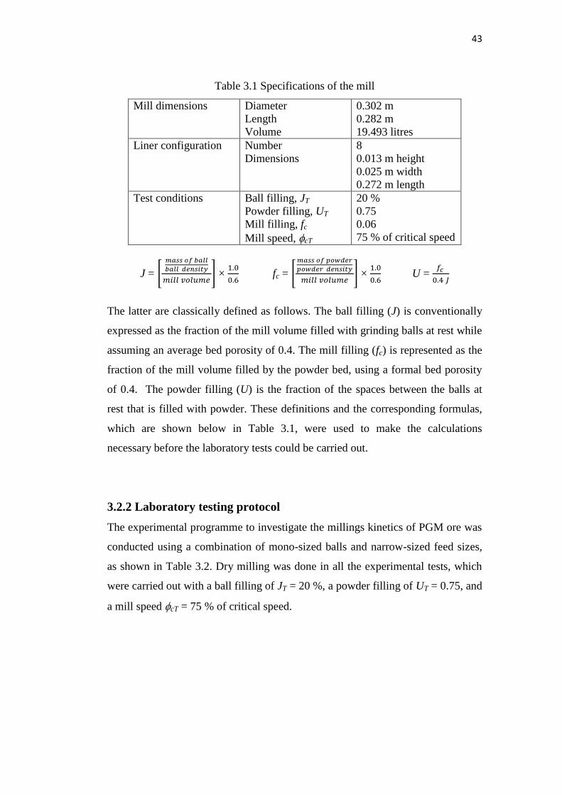
3.2.2 Laboratory testing protocol.....................................................................43
3.3 Feed material preparation.................................................................................44
3.3.1 Feed preparation......................................................................................44
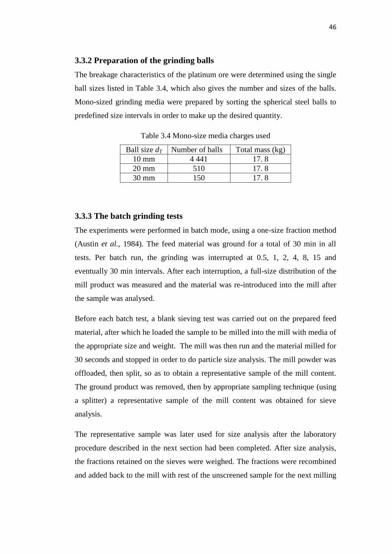
3.3.2 Preparation of grinding balls...................................................................46
3.3.3 The batch grinding tests..........................................................................46
3.3.4 Particle size analysis...............................................................................47
3.3.5 Data collection and processing...............................................................47
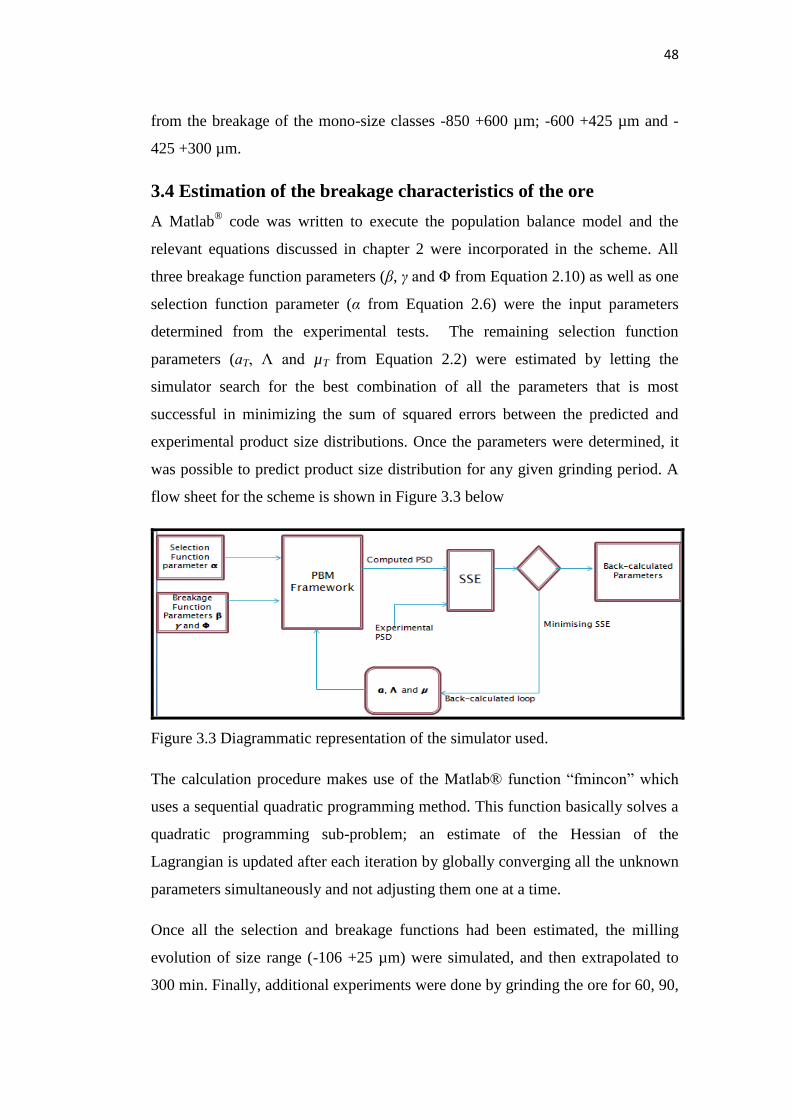
3.4 Estimation of the breakage characteristics of the ore......................................48
3.5 Scale-up Methodology.....................................................................................49
3.5.1 Batch test data.........................................................................................49
3.5.2 The industrial mill...................................................................................49
3.5.3 The scale-up procedure...........................................................................50
3. 6 Simulation of the residence time.....................................................................51
3.7 Simulation of the power draw..........................................................................53
3.8 Summary..........................................................................................................53
Chapter 4 Determination of the milling parameters of a Platinum Group
Minerals ore to optimize product size distribution for flotation
purposes...........................................................................................54
4.1 Introduction.....................................................................................................56
4.2 Results and discussions....................................................................................57
4.2.1 Determination of the selection function parameters……………..…….57
4.2.2 Determination of the breakage function parameters………..………….60
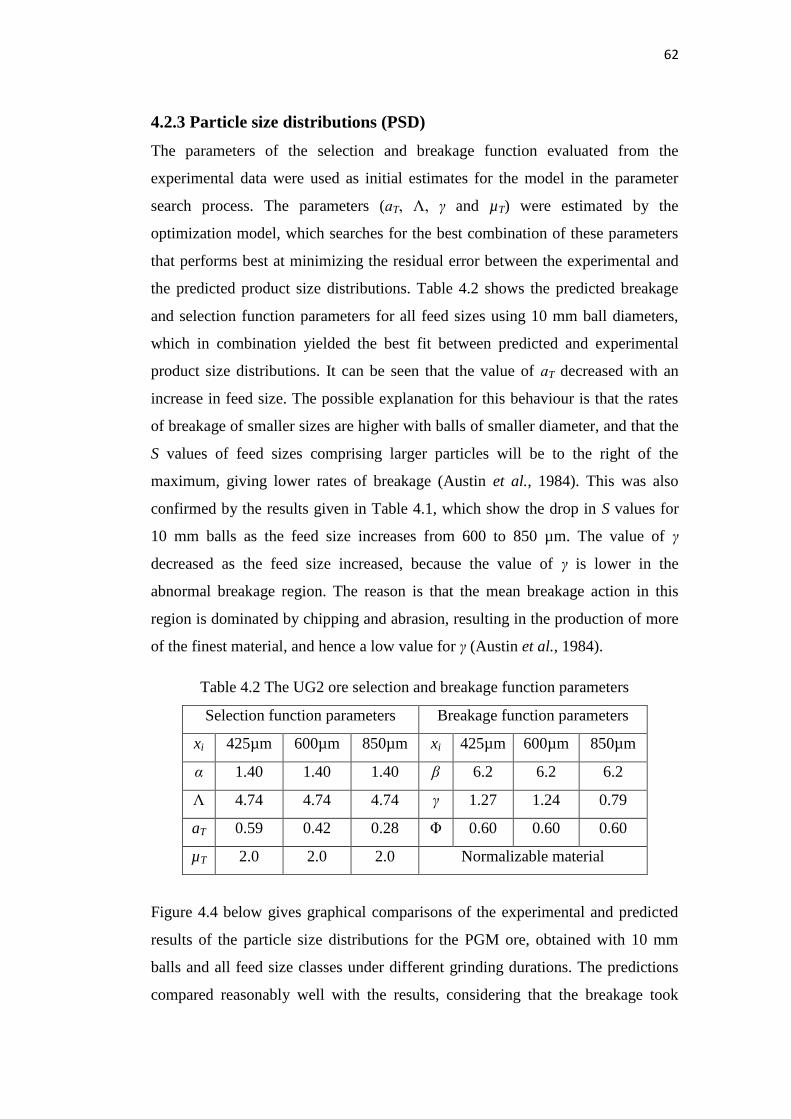
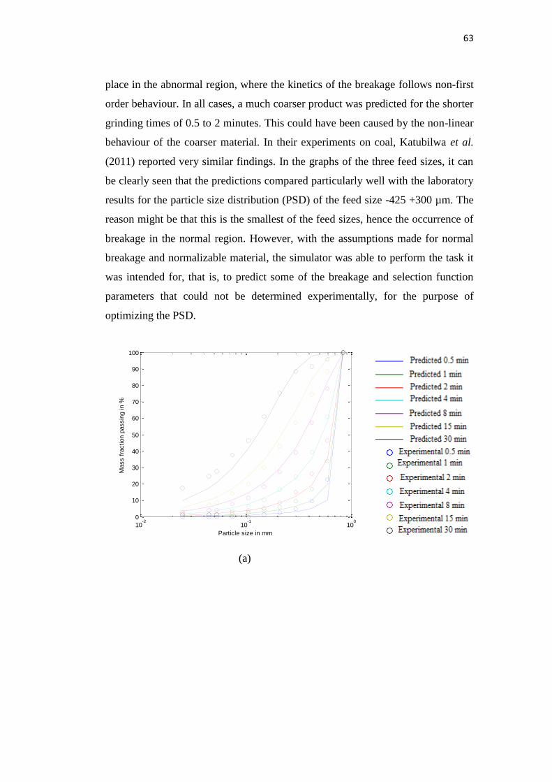
4.2.3 Particle size distributions………………………………………………62
4.3 Conclusion........................................................................................................65
4.4 Summarised findings........................................................................................66
Chapter 5 Scale-up of batch grinding data for simulation of industrial milling
of platinum group minerals ore.......................................................68
5.1 Introduction.....................................................................................................70
5.2 Results and Discussions……………………………………………………...71
5.2.1 Validation of the scale-up procedure……………….………………….72
5.2.2 Using modelling to explore effects of varying operational conditions
……………….………………………………………………………..73
5.2.2.1 Effects of mill speed on milling kinetics......................................73
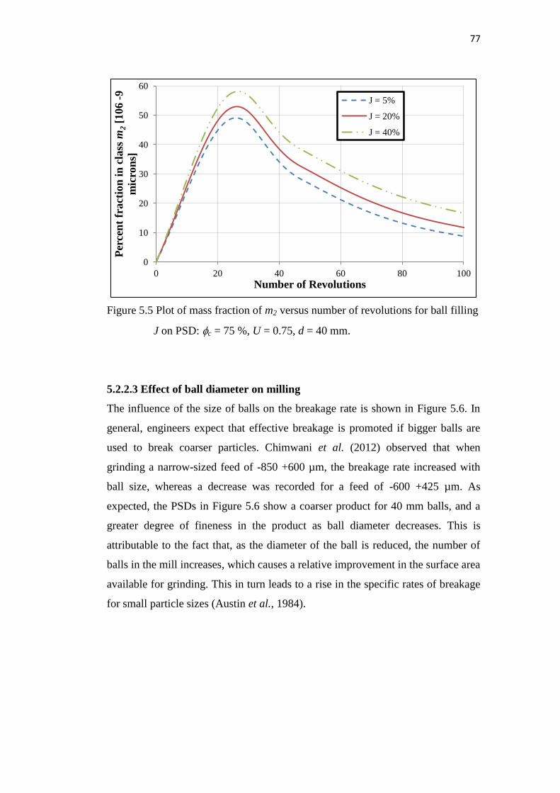
5.2.2.2 Effect of ball filling on milling....................................................76
5.2.2.3 Effect of ball diameter on milling................................................77
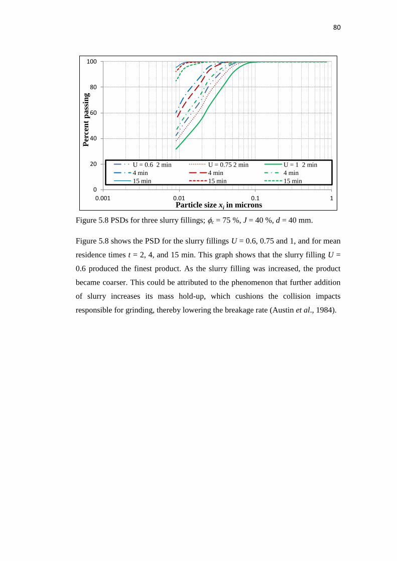
5.2.2.4 Effects of slurry filling on milling...............................................79
Page 10
x
5.3 Conclusion........................................................................................................83
Chapter 6 Use of the attainable region method in determining the optimal
residence time of a ball mill..............................................................85
6.1 Introduction......................................................................................................86
6.2 Data collection and analysis.............................................................................87
6.2.1 Effects of ball filling on mill production...............................................88
6.2.2 Effects of ball size on mill production...................................................92
6.2.3 Effects of mill speed on mill production................................................95
6.3 Summarised findings........................................................................................96
6.4 Conclusion........................................................................................................98
6.5 Future outlook..................................................................................................99
Chapter 7 Use of the attainable region method to simulate a full-scale ball
mill with a realistic transport model.............................................101
7.1 Introduction....................................................................................................103
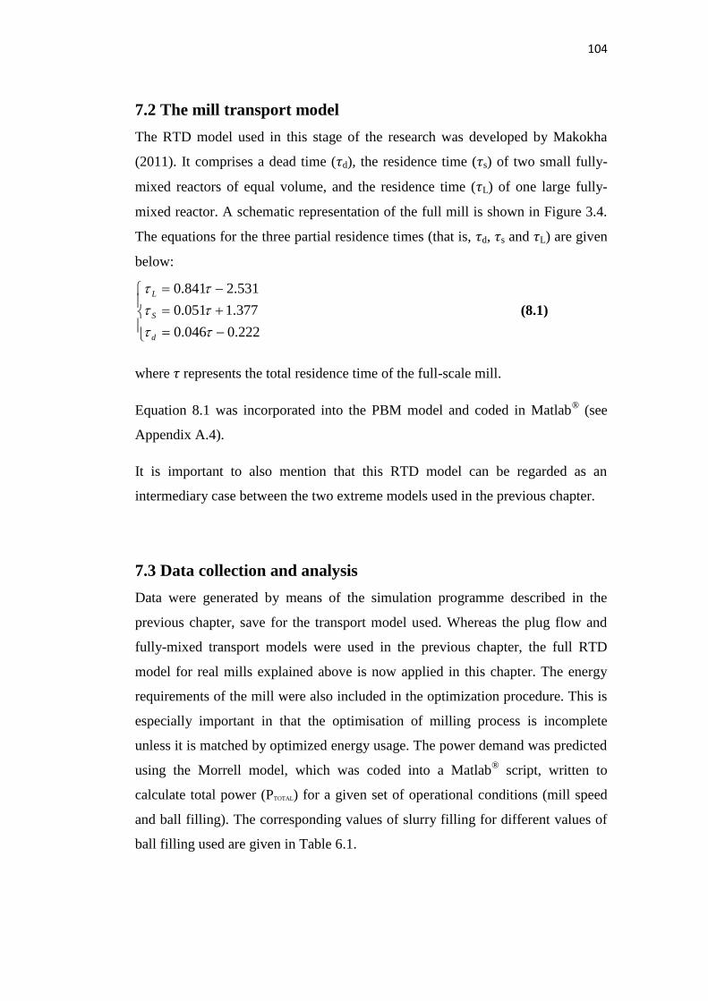
7.2 The mill transport model................................................................................104
7.3 Data collection and analysis...........................................................................104
7.3.1 Effects of ball filling on mill production.............................................105
7.3.2 Effects of ball size on mill production.................................................107
7.3.3 Effects of mill speed on mill production..............................................109
7.4 Energy consumption of the mill.....................................................................110
7.5 Summarised findings......................................................................................114
Chapter 8 Conclusions and recommendations................................................117
8.1 Introduction....................................................................................................117
8.2 Characterisation of the PGM ore....................................................................117
8.3 Extension of the AR region method to continuous milling............................118
8.4 Summary of the major findings......................................................................118
8.5 Overall conclusion.........................................................................................122
8.6 Recommendations for future work................................................................122
List of references................................................................................................124
Appendices..........................................................................................................132
A.1 Batch grinding data.......................................................................................132
A.2 Determination of the milling properties of the ore........................................138
A.2.1 Search engine for population balance model parameters....................138
A.2.1.1 The driver used for the parameter search based on batch
grinding data available……………………………….....……..138
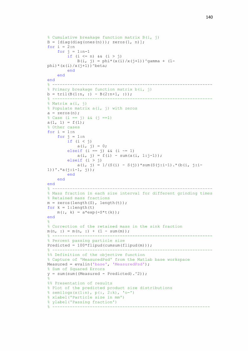
A.2.1.2 The function file for the generation of product side distribution
once PBM parameters are inputted……………………..….139
Page 11
xi
A2.1.3 The plotting facility of the product size distribution based on
back-calculated parameters…………………………………....141
A.2.2 Simulator for the milling kinetics of the size class of interest………143
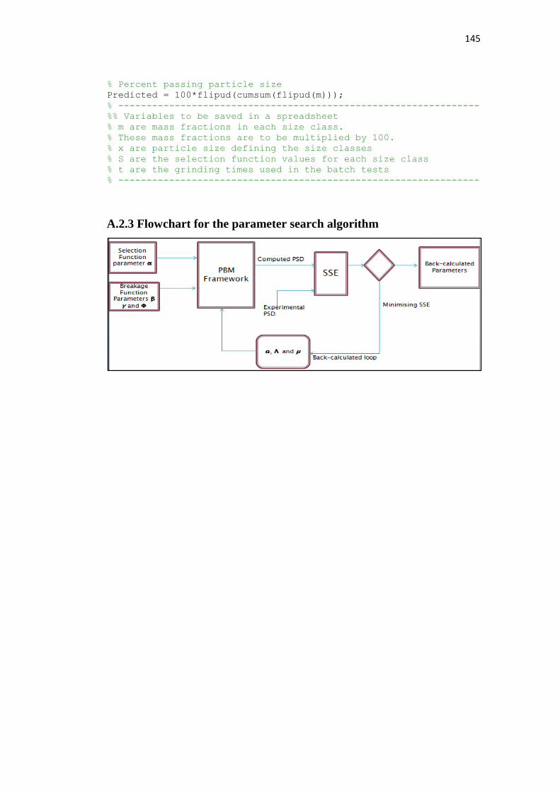
A.2.3 Flowchart for the parameter search algorithm....................................145
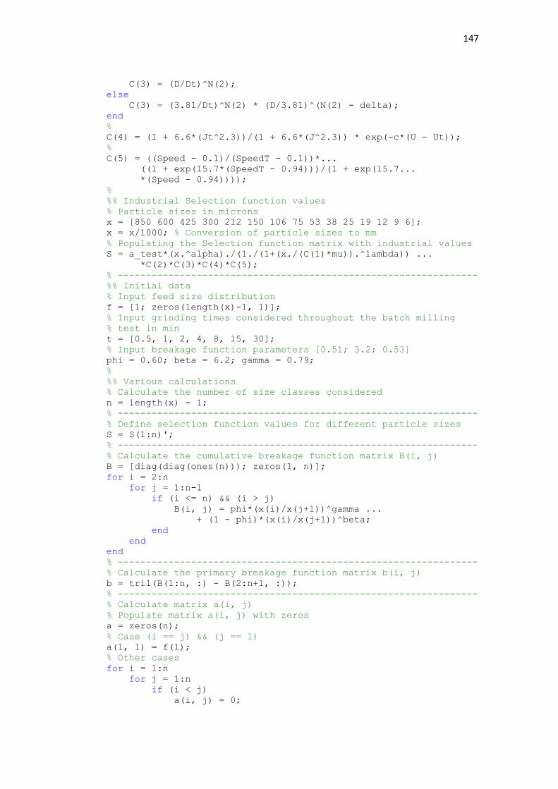
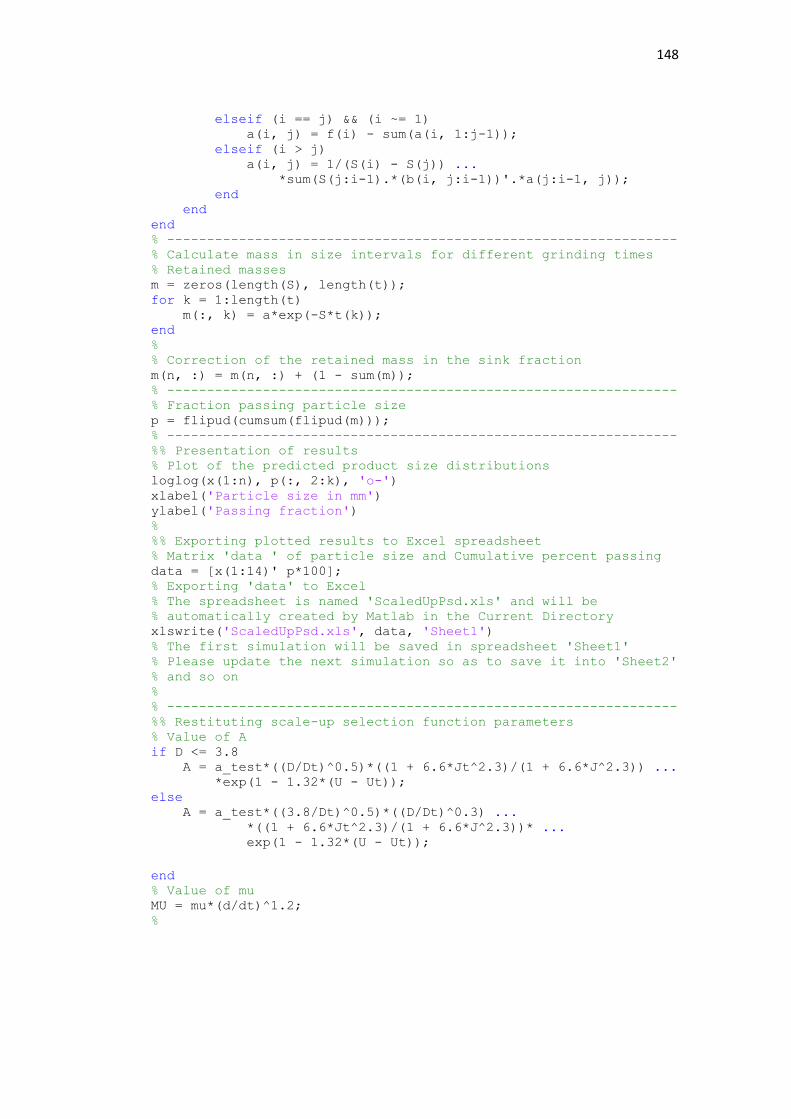
A.3 Scale-up procedure for laboratory-based PBM parameters..........................146
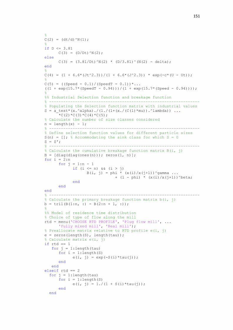
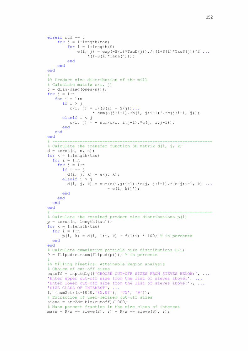
A.4 Optimisation of the residence time................................................................149
A.5 Matlab version of the Morrell power model.................................................154
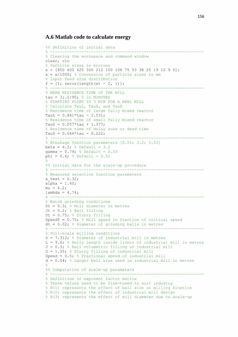
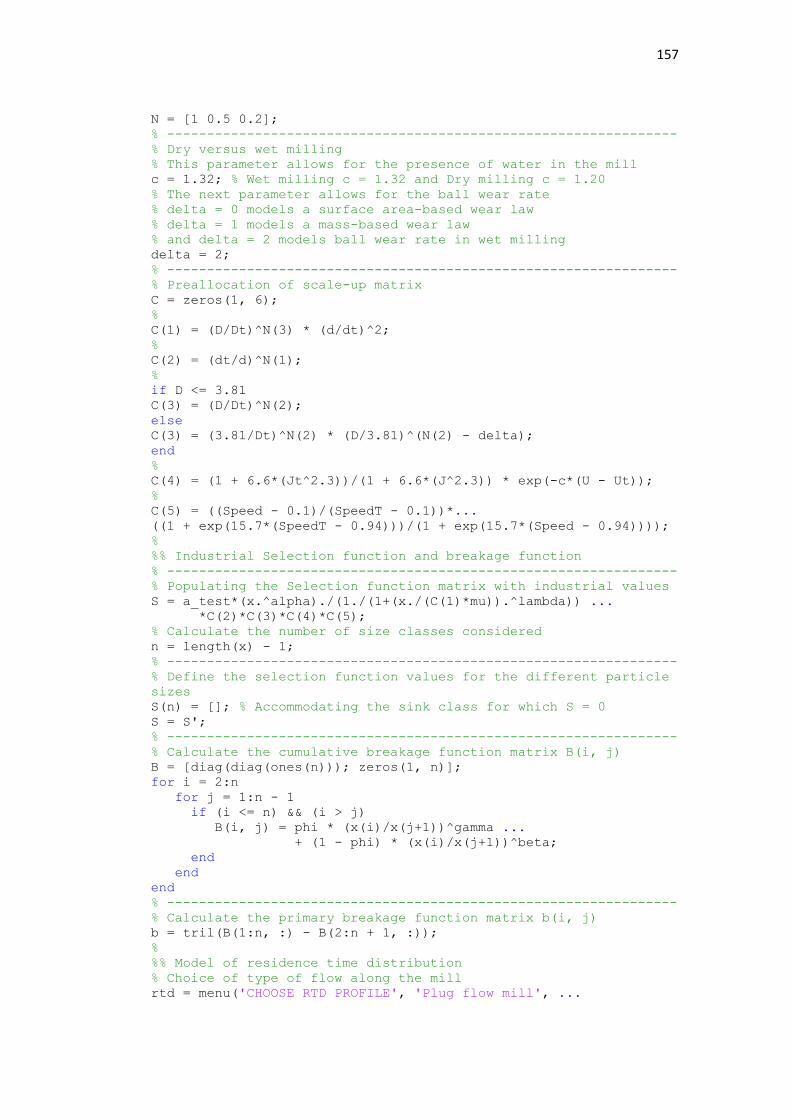
A.6 Matlab code to calculate energy....................................................................156
Page 12
xii
List of figures
Figure 2.1 Schematic illustration of first order plots (Yekeler, 2007).....................9
Figure 2.2 Non-first-order grinding of a narrow-sized feed (Bilgili et al.,
2006)......................................................................................................................10
Figure 2.3 Variation of the selection function with particle size (Austin et al.,
1984)......................................................................................................11
Figure 2.4 Breakage function of typical material (after Yekeler, 2007)................13
Figure 2.5 Illustration of the difference in load behaviour for different ball charge
levels but same mill speed (after Fortsch et al. 2006)...........................20
Figure 2.6 Motion of charge in ball mills (Wills and Napier-Munn, 2006)..........23
Figure 2.7 Ball mill flow regime as a function of increasing speed (after Boateng
and Barr, 1996)......................................................................................24
Figure 2.8 Variation of specific rate of breakage with ball diameter (after Napier-
Munn et al. 1996)..................................................................................26
Figure 2.9 Example of tracer response of a full-scale mill: ball filling J = 25 %
and slurry at 67.3 % solids concentration (after Makokha, 2011)........29
Figure 2.10 RTD’s of a plug-flow, a perfectly mixed and a real ball mill............30
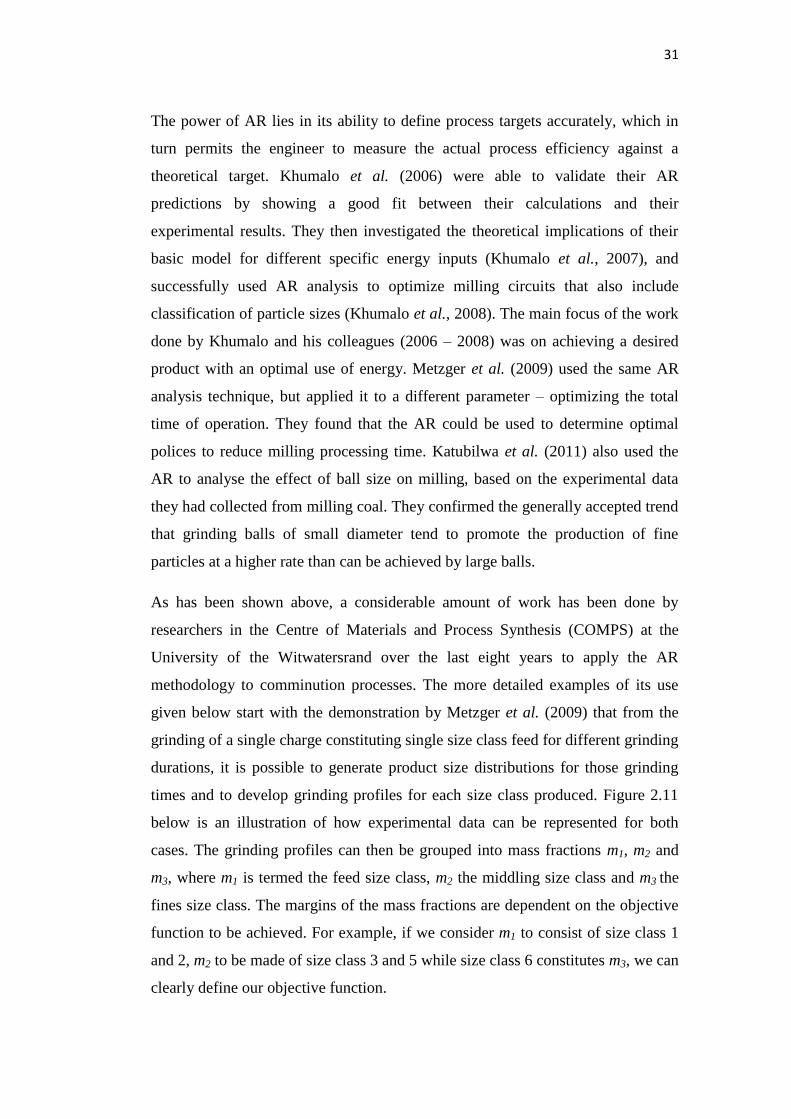
Figure 2.11 (a) Grinding profiles of all six class sizes versus time. (b) Cumulative
mass fraction versus average particle size (Metzger et al. 2009)…...32
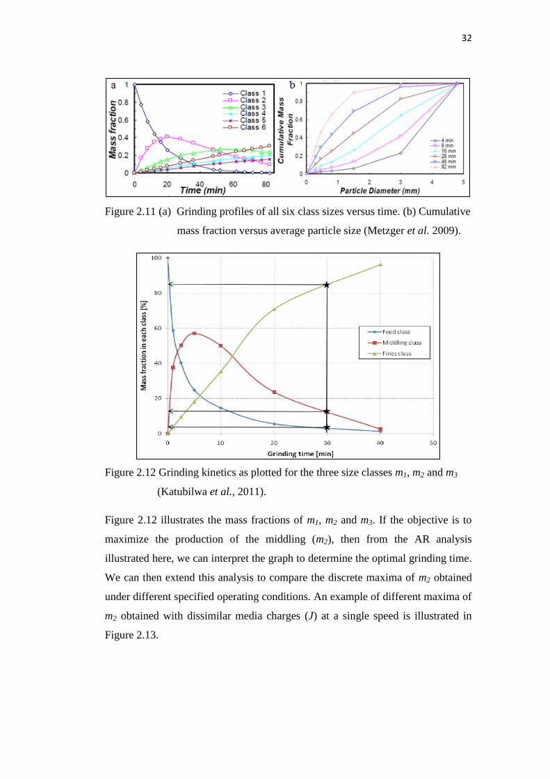
Figure 2.12 Grinding kinetics as plotted for the three size classes m1, m2 and m3
(Katubilwa et al., 2011)......................................................................32
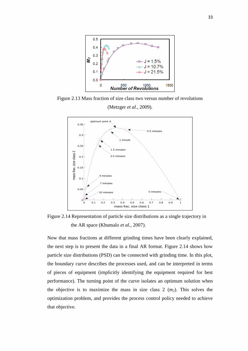
Figure 2.13 Mass fraction of size class two versus number of revolutions
(Metzger et al., 2009)..........................................................................33
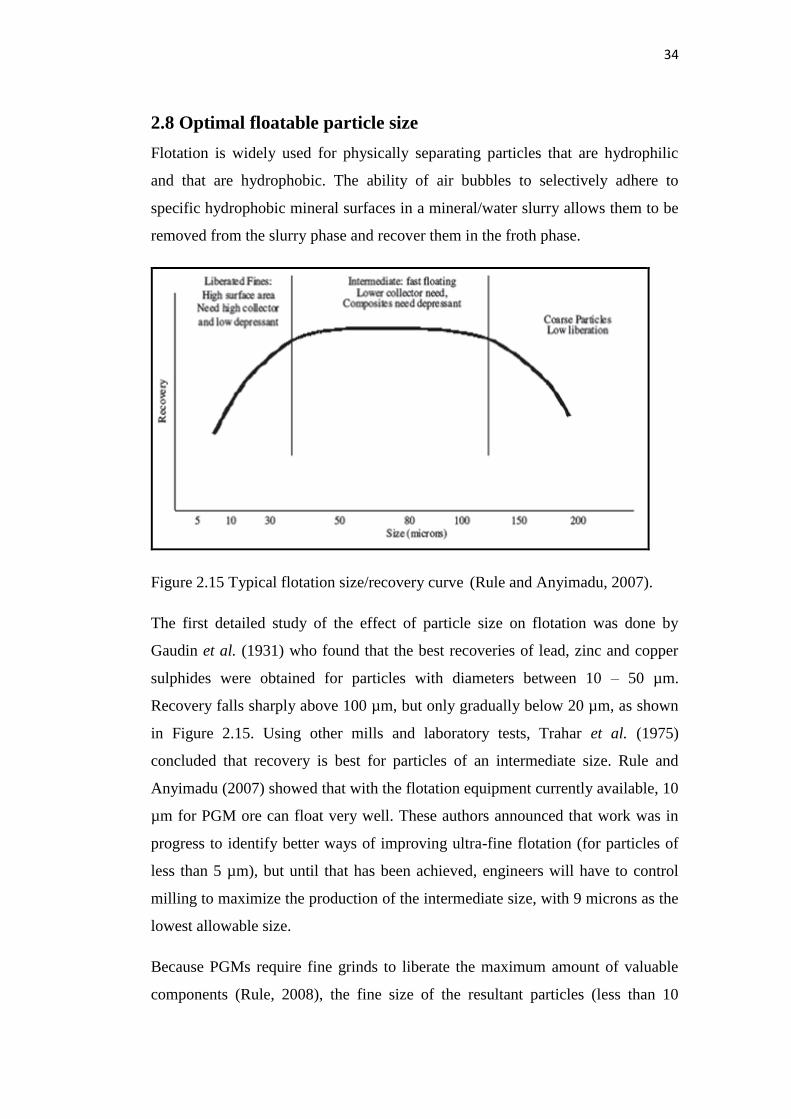
Figure 2.14 Representing particle size distributions as a single trajectory in the
AR space (Khumalo et al., 2007)........................................................33
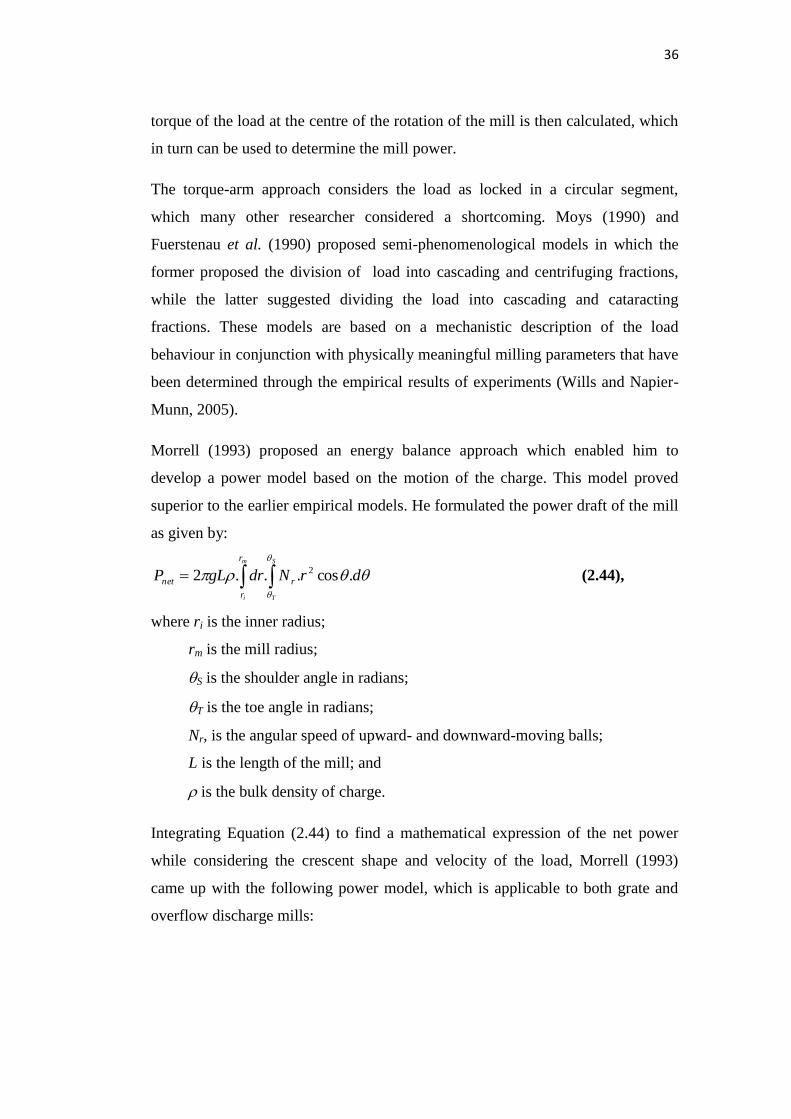
Figure 2.15 Typical flotation size/recovery curve (Rule and Anyimadu, 2007)...34
Figure 2.16 The combined closed circuit (from Austin et al., 1984).....................39
Figure 3.1 View of the laboratory ball mill............................................................42
Figure 3.2 Picture of the laboratory grinding mill used for the experiments.........42
Page 13
xiii
Figure 3.3 Diagrammatic representation of the simulator used.............................48
Figure 3.4 Schematic representation of the tanks in series model with dead time
(after Makokha et al.,2011...…………………………………………51
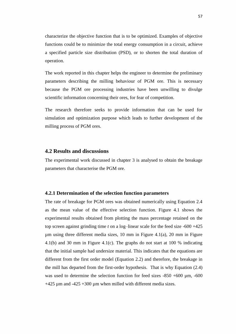
Figure 4.1 First-order plot for UG2 ore mono-size class (-600 +425 µm) ground
with different media sizes (dT): (a) 10 mm; (b) 20 mm; (c) 30 mm......58
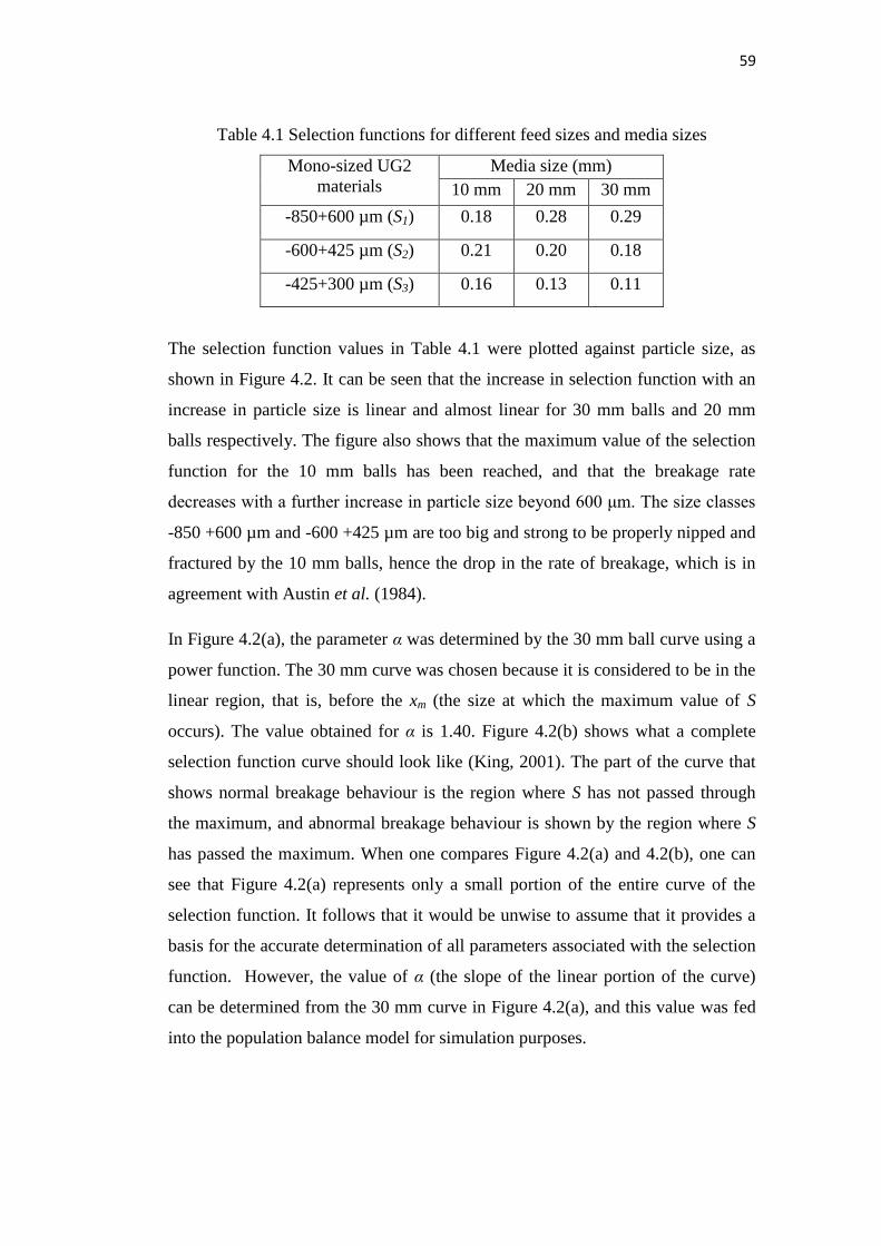
Figure 4.2 (a) Variation of S with particle size (b) Graphical procedure for the
determination of the parameters (Austin et al. 1984)............................60
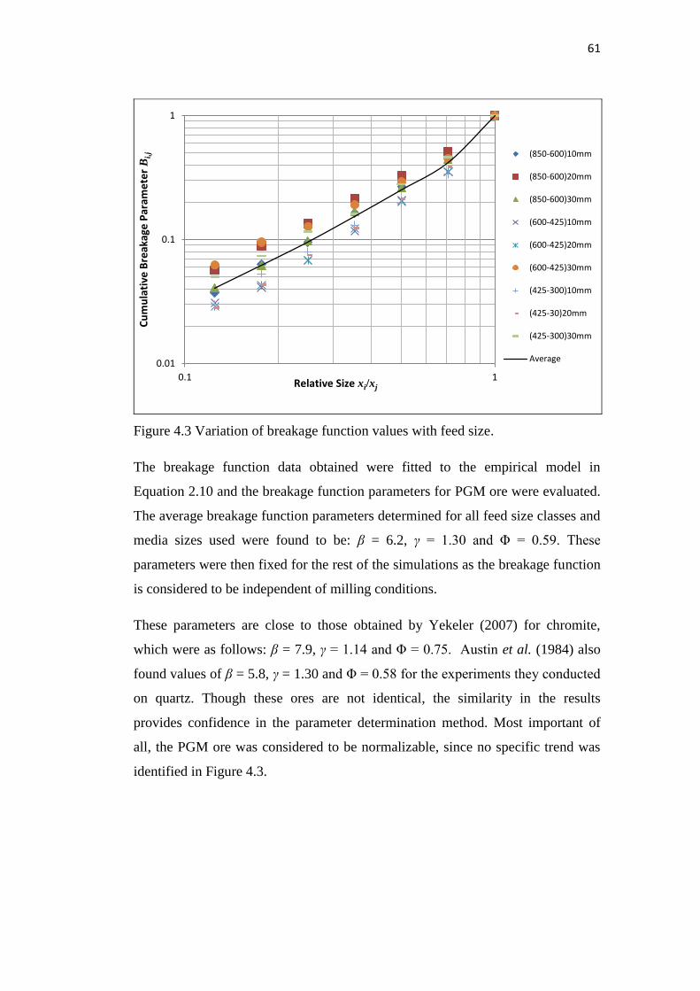
Figure 4.3 Variation of breakage function values with feed size...........................61
Figure 4.4 Measured and predicted particle size distributions corresponding to 10
mm ball size and feed sizes: (a) -850 +600 µm (b) -600 +425 µm and
(c) -425 +300 µm.............................................................................63-64
Figure 4.5 Milling kinetics of the desired size class for 20 mm balls and feed size
-850 +650 µm......................................................................................65
Figure 5.1 Comparison between experimentally measured data and the predicted
PSD using the scale up method for the large scale mill: (a) J = 24.6 %
and 74.5 % solids, (b) J = 32.9 % and 67.7 % solids, (c) J = 32.8 % and
65.1 % solids, (d) J = 32.9 % and 72.1 % solids.....................................73
Figure 5.2 Predicted PSD’s for four mill speeds: J = 40%, U = 0.75, d = 40 mm
and varying residence times..................................................................74
Figure 5.3 Plot of mass fraction of m2 versus number of revolutions for different
speeds c; J = 40 %, U = 0.75, and d = 40 mm……………...............75
Figure 5.4 Effect of ball filling J on PSD: c = 75 %, U = 0.75, d = 40
mm........................................................................................................76
Figure 5.5 Plot of mass fraction of m2 versus number of revolutions for ball filling
J on PSD: c = 75 %, U = 0.75, d = 40 mm………………….………..77
Figure 5.6 PSD for different media sizes;c = 75 %, U = 0.75, J = 40 %..............78
Figure 5.7 Plot of mass fraction of m2 versus number of revolutions for different
ball sizes; J = 40 %, c = 75 %, U = 0.75…………………….……….79
Figure 5.8 PSDs for three slurry fillings; c = 75 %, J = 40 %, d = 40
mm.........................................................................................................80
Figure 5. 9 Plot of mass fraction of m2 versus number of revolutions for different
slurry fillings; J = 40 %, c = 75 %, and d = 40 mm…………….........81
Page 14
xiv
Figure 5.10 Summary of various simulations, optimised solution and industrial
operating conditions………………………………………………..82
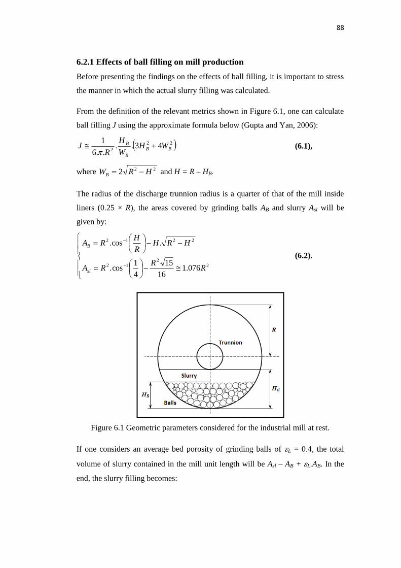
Figure 6.1 Geometric parameters considered for the industrial mill at rest……...88
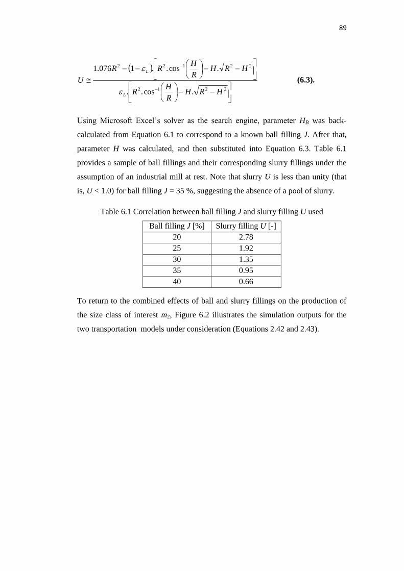
Figure 6.2 Throughput of the mill for the two RTD profiles. Simulation
conditions: J = 30 %, U = 1.35, d = 40 mm and c = 70 %
critical……...……………………………………………………..…90
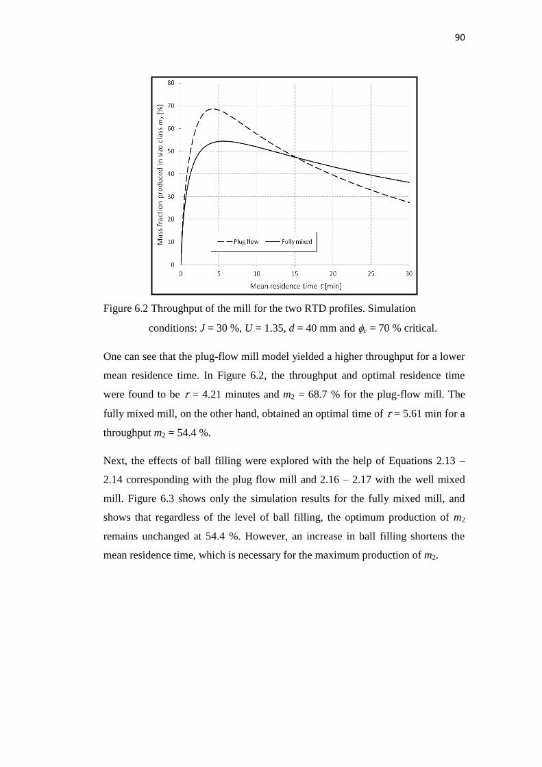
Figure 6.3 Prediction of ball filling effects on mill throughput for a fully mixed
mill. Simulation conditions: d = 40 mm and c = 70 % of critical…..91
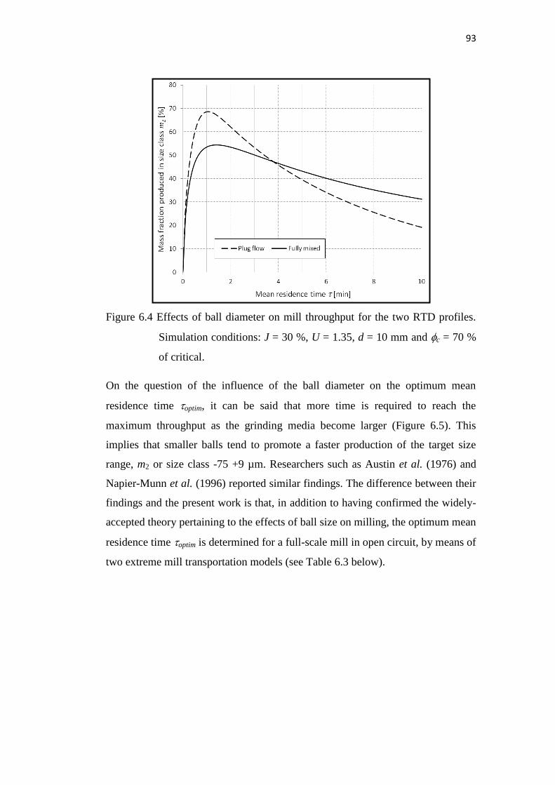
Figure 6.4 Effects of ball diameter on mill throughput for the two RTD profiles.
Simulation conditions: J = 30 %, U = 1.35, d = 10 mm and c = 70 % of
critical....................................................................................................93
Figure 6.5 Effects of ball size on mill throughput for a well-mixed mill.
Simulation conditions: J = 30 %, U = 1.35, and c = 70 % of critical..94
Figure 6.6 Effects of mill speed on mill throughput for a fully mixed mill.
Simulation conditions: J = 25 %, U = 1.92 and d = 30 mm..................95
Figure 6.7 Residence time optim as a function of mill speed c for J = 30 % under
varying ball diameters. Solid and dashed lines in the plot area represent
the well-mixed and plug-flow mill models respectively.......................98
Figure 7.2 Throughput profiles of the mill for the three transport models.
Simulation conditions: J = 30 %, U = 1.35, d = 40 mm and c = 70 % of
critical..................................................................................................105
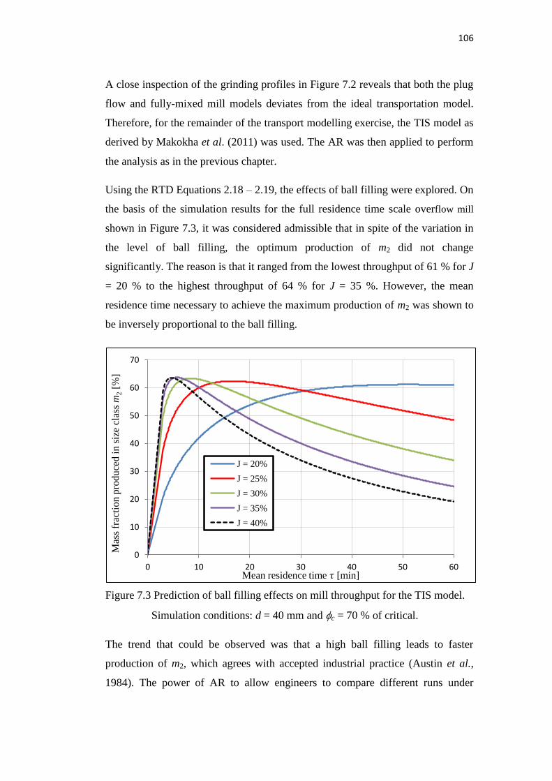
Figure 7.3 Prediction of ball filling effects on mill throughput for the TIS model.
Simulation conditions: d = 40 mm and c = 70 % of critical..............106
Figure 7.4 Effects of ball size on mill throughput for the TIS model. Simulation
conditions: J = 25 %, U = 1.92, and c = 70 % of critical...................108
Figure 7.5 Effects of mill speed on mill throughput for the TIS model. Simulation
conditions: J = 30 %, U = 1.35 and d = 40 mm...................................109
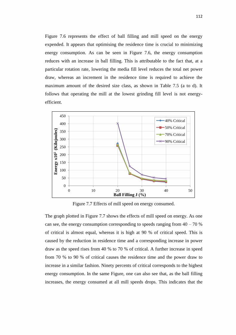
Figure 7.6 Effects of ball filling on energy..........................................................111
Figure 7.7 Effects of mill speed on energy consumed.........................................112
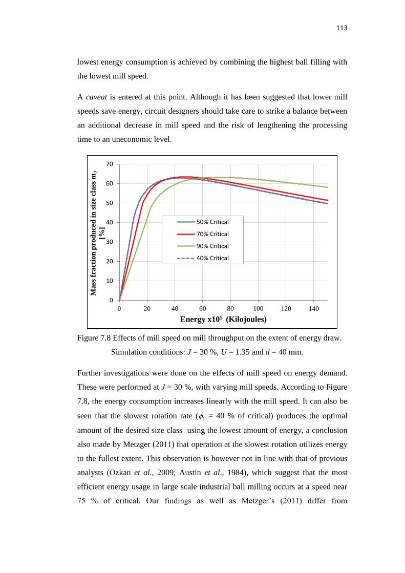
Figure 7.8 Effects of mill speed on mill throughput on the extent of energy draw.
Simulation conditions: J = 30 %, U = 1.35 and d = 40 mm................113
Page 15
xv
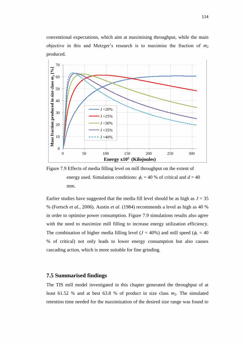
Figure 7.9 Effects of media filling level on mill throughput on the extent of
energy used. Simulation conditions: c = 40 % of critical and d = 40
mm.......................................................................................................114
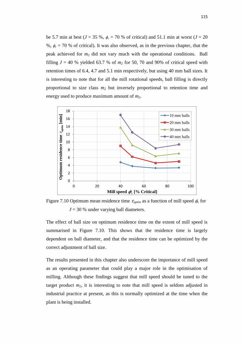
Figure 7.10 Optimum mean residence time optim as a function of mill speed c for
J = 30 % under varying ball diameters................................................115
Figure 7.11 Optimal residence time versus ball filling at different speeds.........116
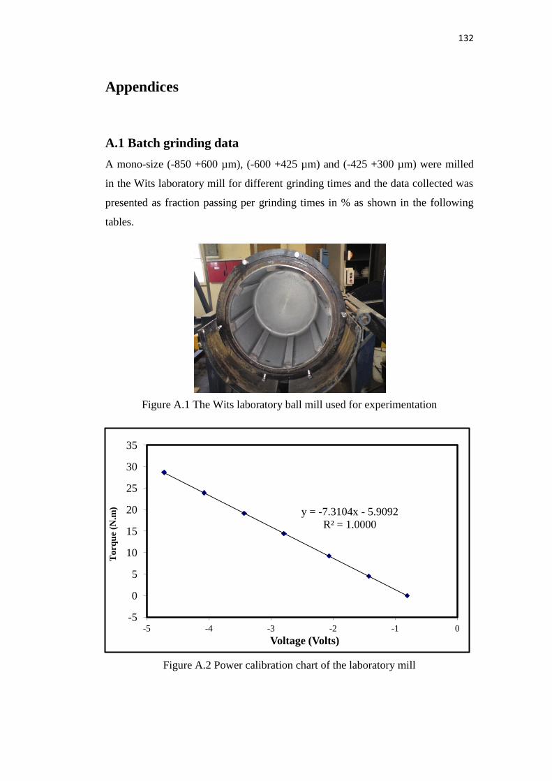
Figure A.1 The Wits laboratory ball mill used for experimentation....................132
Figure A.2 Power calibration chart of the laboratory mill...................................132
A.2.3 Flowchart for the parameter search algorithm……………………….......145
Page 16
xvi
List of tables
Table 3.1 Specifications of the mill.......................................................................43
Table 3.2 Experimental design...............................................................................44
Table 3.3 Mass retained on each sieve at different times…………………..……45
Table 3.4 Mono-size media charges used..............................................................46
Table 4.1 Selection functions for different feed sizes and media sizes.................59
Table 4.2 The UG2 ore selection and breakage function parameters....................62
Table 5.1 Breakage parameters as scaled-up to industrial mill..............................72
Table 5.2 Individual milling parameters and corresponding optimum
throughput.............................................................................................82
Table 6.1 Correlation between ball filling J and slurry filling U used..................89
Table 6.2 Mean residence times optim for d = 40 mm and c = 70 % of critical....91
Table 6.3 Mean residence times optim for J = 30 % and c = 70 % of critical.......94
Table 6.4 Optimum mean residence times optim for J = 25 % and d = 30 mm......95
Table 7.1 Mean residence times optim for d = 40 mm and c = 70 % of critical..107
Table 7.2 Mean residence times optim for J = 25 % and c = 70 % of critical.....108
Table 7.3 Optimum mean residence times optim for J = 30 % and d = 40 mm....109
Table 7.4 Optimal residence time, net power and energy of 40 mm ball size for
varying fraction of speed and ball filling.....................................110-111
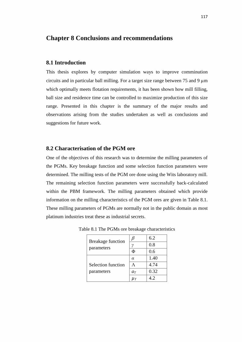
Table 8.1 The PGMs ore breakage characteristics...............................................117
Table A.1 Measured particle size distribution for ball size 10 mm, feed size (-850
+600 m), U = 0.75, J = 20 %, c = 75 of critical, fc = 0.06...............133
Table A.2 Measured particle size distribution for ball size 10 mm, feed size (-600
+425 m), U = 0.75, J = 20 %, c = 75 of critical, fc = 0.06...............133
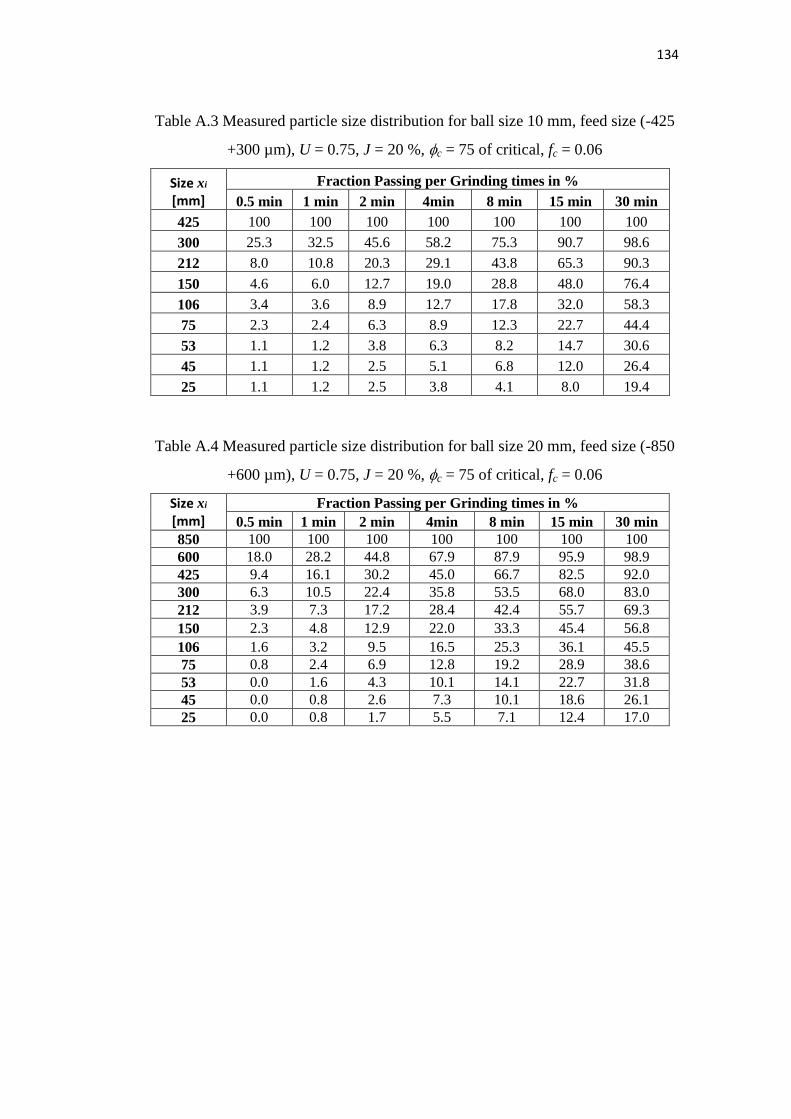
Table A.3 Measured particle size distribution for ball size 10 mm, feed size (-425
+300 m), U = 0.75, J = 20 %, c = 75 of critical, fc = 0.06...............134
Table A.4 Measured particle size distribution for ball size 20 mm, feed size (-850
+600 m), U = 0.75, J = 20 %, c = 75 of critical, fc = 0.06...............134
Table A.5 Measured particle size distribution for ball size 20 mm, feed size (-600
+425 m), U = 0.75, J = 20 %, c = 75 of critical, fc = 0.06...............135
Page 17
xvii
Table A.6 Measured particle size distribution for ball size 20 mm, feed size (-425
+300 m), U = 0.75, J = 20 %, c = 75 of critical, fc = 0.06...............135
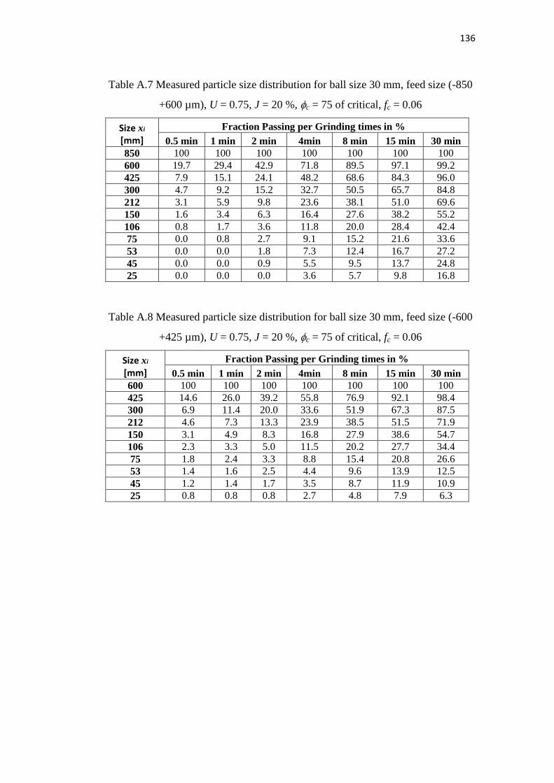
Table A.7 Measured particle size distribution for ball size 30 mm, feed size (-850
+600 m), U = 0.75, J = 20 %, c = 75 of critical, fc = 0.06...............136
Table A.8 Measured particle size distribution for ball size 30 mm, feed size (-600
+425 m), U = 0.75, J = 20 %, c = 75 of critical, fc = 0.06...............136
Table A.9 Measured particle size distribution for ball size 30 mm, feed size (-425
+300 m), U = 0.75, J = 20 %, c = 75 of critical, fc = 0.06...............137
Table A.10 Breakage function values calculated using the BII-method from
laboratory data and later used to determine breakage function
parameters....................................................................................137-138
Table A.11 Breakage parameters as scaled-up to industrial mill.........................149
Table A.12 Measured versus scaled-up particle size distributions......................149
Page 18
1
Chapter 1 Introduction
1.1 Background and Motivation
Milling is an operation widely used in the mineral, metallurgical, power
generation and chemical industries. One of the primary reasons for choosing to
mill materials to smaller sizes is to liberate valuable components that are
dispersed in the host matrix. Once the material has been broken and sufficient of
these components have been liberated, they are separated from the valueless
remainder by downstream processes such as flotation. The effectiveness of the
downstream process is therefore dependent on the milling process. That is the
reason why it is necessary to tailor the milling parameters to obtain products that
are best suited to the requirements of the downstream process concerned. For
instance flotation, the particle size range has to be such that over-grinding is
avoided on one hand which is a waste of energy and on the other under-grinding
that leaves most mineral value unliberated resulting in low mineral recovery
during the separation process is also undesirable. The application of
comprehensive mathematical milling models is useful in targeting the flotation
size requirements better.
The most commonly-accepted milling model follows the Population Balance
Model (PBM) framework (Yekeler, 2007), which is based on the first-order law of
kinetics. In this model, particles in a narrow size interval are assumed to break
proportionally to their mass fraction (Reid, 1965; Kelsall and Reid, 1965; Austin,
1971; Mika, 1975). By performing a size-mass balance in narrow size intervals, it
is possible to describe milling in a time domain (Koka and Trass, 1988), which
makes it possible to determine the product size distribution after a given grinding
time.
The assumption of first-order breakage suggests that ball milling can be
represented in a mode similar to the expression of chemical reactions (Khumalo et
al., 2006 – 2008). Consequently, an analytical tool known as the Attainable
Region (AR) can be used to study milling. Initially proposed for the analysis of
Page 19
2
chemical engineering systems, the AR technique has been successfully extended
to comminution (Khumalo, 2007; Khumalo et al., 2006 – 2008; Metzger, 2011;
Metzger et al., 2009 & 2011; Katubilwa et al., 2011, Chimwani et al., 2012).
The successful use of the AR technique to determine the set of all achievable
distributions for the process conditions has already been demonstrated. Although
most of the work done so far has been laboratory-based, the results have been
encouraging. That is why the present thesis seeks to extend the methodology to
full scale milling. To accomplish this, data collected from batch grinding tests was
scaled up to an industrial mill that had been surveyed and the data were explored
further to arrive at best milling option that met the flotation size requirements. The
intention was to determine a milling circuit that would produce optimal flotation
sizes in the milled ore. The sampling work of the referred industrial mill was
published before (Makokha, 2012). It is shown that improved milling efficiency
could be achieved through optimal residence time.
1.2 Problem statement
The most common processing challenges encountered when liberating Platinum
Group Mineral (PGM) ores are generally associated with the fineness and gangue
association of mineral species (Cramer, 2001). In a typical South African
scenario, PGM ores are milled before being sent for flotation. In such a case, one
of the reasons for a low flotation recovery could be the failure of the last stage of
milling to generate a sufficient percentage of particles within the floatable size
range. It is therefore understood that optimizing the milling stage could be one
way of improving flotation efficiency. However, in order to optimize milling, it is
necessary to start by establishing the optimum flotation requirements in terms of
floatable particle sizes. Then, using the AR technique, this information can be
used to determine how the milling can be adapted to provide a more appropriate
feed for the flotation section. The key issue is therefore to develop a robust AR
framework applicable to continuous milling. Having achieved this, the final task
will be to ascertain whether the laboratory-based findings can be extended to full-
scale milling.
Page 20
3
It has been shown at the laboratory scale using the AR technique that a substantial
amount of energy can be saved, while still ensuring effective grinding, through
controlled classification (Khumalo et al., 2008). Common practice, however,
continues to follow the assumption that the higher the energy consumption, the
higher the milling rate (Austin et al., 1984; Wills and Napier-Munn, 2005). It has
also been shown that less powder and fewer grinding balls can bring about more
effective grinding (Metzger et al., 2011). Conventional practice, on the other
hand, favours mills with high ball loading J and powder filling U close to unity
(that is U 1) (Tangsathitkulchai, 2003; Latchireddi and Morrell, 2003). Finally,
low-speed mills have been shown to bring about a high product fineness at the
same rate as (and sometimes at a higher rate than) high-speed mills (Metzger,
2011); whereas, once more, traditional practice proposes speeds nearing 75 % as
critical to guarantee high power draw and therefore more grinding at a faster rate
(Austin et al., 1984; Wills and Napier-Munn, 2005).
All of the above suggests that the innovations prompted by the AR approach
contradict the milling conditions under which most of the concentrators operate.
The main problem is that all of the AR-related claims have so far been based on
laboratory batch investigations (Khumalo, 2007; Khumalo et al., 2006 – 2008;
Metzger, 2011; Metzger et al., 2009 & 2011; Katubilwa et al., 2011), and as such,
their validity has been limited by the scale factor. In addressing this issue, a
convincing answer has to be provided to a key question: Can the attainable region
technique be extended to industrial conditions of a full scale mill and be used to
optimise flotation feed size distribution? If this can be answered in the
affirmative, then the corollary to this question would be to propose the AR as an
alternative and complementary analytical tool for the optimization of milling
circuits.
1.3 Research objectives and envisaged contribution
This research was intended to apply various aspects of industrial ball milling that
could be used to control and optimize the performance of a milling circuit. The
desired end result was to generate the maximum production of preselected sizes
Page 21
4
for flotation or floatable particle sizes. The AR approach was used to optimize the
operational parameters as well as the residence time of a full-scale industrial mill.
The breakage and selection function parameters of a PGM ore were measured by
means of laboratory batch grinding tests, and the resultant parameters were scaled
up using empirical scale-up models (Austin et al., 1984). After that, the influence
of the various milling parameters on the mill circuit and on size distribution of the
final product was assessed by simulation.
The research set out in this thesis is expected to provide information on the
milling characteristics of PGM ores in general. This is important, since these data
have not been generally available to the public at large. The milling data can be
used for simulation and optimization purposes, and may lead to further
investigations of PGM milling. In addition, the research establishes a precedent
for the use of the AR technique in the minerals industry as a tool of choice for the
analysis and optimization of mineral processing circuits.
1.4 Layout of the dissertation
The thesis is organized into eight chapters, including the introduction. In the
introductory chapter, the background and motivation are presented as well as the
problem statement and research objectives on which the thesis is based.
The second chapter presents a review of the studies accomplished to date
regarding comminution modelling. It reviews the population balance modelling of
ball mills. It also gives a description of the attainable region approach, to provide
a context for the research work reported in the chapters that follow.
The third chapter comprises a detailed description of the experimental equipment,
the data collection methods used in the work undertaken, and the simulation
strategy used to assess whether the objectives of this study had been met.
Chapter four recounts how a set of batch milling parameters were established for
the platinum group mineral ore. Some of the breakage parameters were measured
directly in the laboratory, while the remaining breakage parameters were back-
Page 22
5
calculated within the population balance model framework. These parameters
provide a basis for simulation and optimization of the milling process in the
subsequent chapters. Validation of these parameters is also done in the same
chapter.
Chapter five records the process by which the batch milling parameters were
scaled up from laboratory to full operation. The data generated was validated
against industrial mill data before the AR technique was used to optimize a range
of industrial milling conditions. These included ball filling (J), mill speed (c),
ball size (d) and powder filling (U). The optimization was centred on the
production of a particle size amenable to efficient flotation.
Chapter six introduces the optimization of residence time as a function of mill
speed (c), ball filling (J), slurry filling (U) and ball size (d). Two mill transport
models are considered: the plug flow model and the perfectly mixed mill model.
Using these simple models, it is possible to determine how a variation in each of
the milling conditions considered affects the production of floatable mill product
from an AR point of view.
Chapter seven is an extension of the sixth chapter. It contains a description of the
application of AR methodology to determine the optimal residence time of a full-
scale mill that incorporates a more realistic transport model based on data
concerning residence time distribution collected from a full-scale mill; attempts
made to optimise the mill product relative to flotation requirements; and
assessment of the energy requirements of the optimized mill. The results are taken
to underscore the power of the AR method as an optimization tool.
Chapter eight contains a summary of the major findings and conclusions drawn
from the work described in this thesis. Recommendations for future work are also
listed.
Page 23
6
Chapter 2 Literature Review
2.1 Introduction
The designers of industrial mills used for mineral extraction aim to create
operational conditions that guarantee high mineral recovery and low costs. In
order to achieve these ends, they normally consider two objective functions: the
energy consumption and the product size relative to a chosen downstream process.
The key aspects of meeting these requirements, as far as grinding and flotation are
concerned, would be the effective control of the desired mill product without
overgrinding or under-grinding.
McIvor and Finch (1991) showed that the relationship between particle size and
flotation performance can be used as a basis for both technical and economic
analyses of the viability of a plant. In terms of particle size, the population balance
model provides a robust formulation of the milling process, and years of
experimentation have confirmed its value (Herbst and Fuerstenau 1980; Herbst et
al., 1981; Austin et al., 1984; Rajamani, 1991; King, 2001). More recently, the
AR concept has been introduced as a graphical technique for the analysis of
milling, and has already proved its relevance as an optimization tool. The
technique can be used to highlight the overall picture of what the data is saying
and help in identifying opportunities that can lead to optimisation. While it is
recognised that flotation is a complex process that is affected by many factors, as
far as milling is concerned, controlling the size distribution of the feed to flotation
is a key role of the milling process.
To provide a perspective on how milling should be tailored to flotation, the work
done by previous researchers on milling was reviewed, and the variety of
technical models they have introduced for analytical and evaluative purposes.
These include the population balance model, the batch grinding equation and the
scale-up procedure for batch grinding data. The product size requirements for
optimal flotation was also discussed, and a detailed introduction to the attainable
region technique given.
Page 24
7
2.2 Theory of milling
In comminution, mathematical relations between feed size and product can be
developed by applying a size mass balance to the milling operation. This is made
possible by the definition of two actions taking place simultaneously inside the
mill: the selection of particles for breakage and the breakage distribution of
‘children’ particles as a result of broken ‘parent’ particles (Gupta and Yan, 2006).
The selection and breakage function are used to investigate the kinetics of size
reduction in tumbling mills (Austin, 1971; Lucky et al., 1972). These two
functions have led to the establishment of the population balance model, which
provides the basis for the modelling of the grinding process. It describes material
breakage in mills based on size-mass balances on narrow size intervals of the
particulate mass. The particulate masses are subjected to breakage in the mill and
are formulated in terms of the selection and the breakage function parameters
(Koka and Trass, 1988). These two actions are discussed in detail in the sections
that follow.
2.2.1 Selection function
The selection function, also called the breakage rate, can be defined as the rate at
which material is broken out of a particular discretized size class.
To explain the concept more fully, a wide range of particle sizes is split into a
number of size intervals following a sequence of sieves. The top size interval
is numbered size class 1, the second is class 2, and so on down to the nth
interval,
which is the final size interval. Now, when one considers the breakage rate of size
class 1 to smaller size classes in a fully mixed batch mill, if the disappearance of
particles per unit time and unit mass due to breakage is proportional to the
instantaneous mass fraction of particles of that size fraction that are present inside
the mill, the breakage is said to follow the first-order law of kinetics.
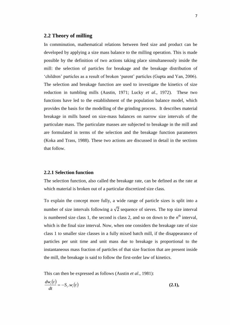
This can then be expressed as follows (Austin et al., 1981):
twS
dt
tdwii
i . (2.1),
Page 25
8
where Si is the rate of disappearance of particles or the selection function;
wi is the mass fraction present in the size interval i after grinding time t; and
i is an integer defining the different size intervals, the largest being 1.
If the breakage rate function (Si) is constant over time as the contents of the mill
become finer, Equation 2.1 integrates to what is known as the “first-order rate
model of grinding” (Napier-Munn et al., 1996):
tSewtw
.
111.
(2.2),
where w1 is the mass fraction present in the size interval 1 after grinding time t.
Equation (2.1) has been found to apply to different types of materials and has
worked well for many materials over a wide range of operations (Austin et al.,
1976; Austin et al., 1984, Bilgili et al., 2006). However, several researchers have
also reported and investigated departures from the first-order breakage pattern.
The following non-exhaustive list of references provides a detailed description of
non-first-order milling kinetics: Austin et al., 1973; Austin et al., 1977; Bilgili and
Scarlett, 2005; Bilgili et al., 2006; Bilgili, 2007; Capece et al., 2011. Suffice it to
say that non-first-order grinding generally occurs when coarse particles are being
milled. In that case, the breakage is referred to as abnormal.
Austin et al. (1977) studied abnormal breakage and postulated that during
grinding, some material that is initially soft breaks down into a component
resistant to further breakage. They proposed the following non-first-order model:
tS
i
tS
iihardsoft ee
m
tmtw
....1
0
(2.3),
where hardsoft
softii
iSS
Sb
.
Ssoft is the selection function of the easy-to-break component of the material;
Shard is the selection function of the hard-to-break component of the feed.
The system behaves as if the material consists of a fraction 1 - of soft
component and a fraction of the hard component. The mean value of the
effective selection function is given by:
Page 26
9
ihard
ii
isoft
i
S
b
S
S
,,
1
1
(2.4).
Figure 2.1 below illustrates a good agreement between the first-order breakage
model and laboratory batch grinding results for a given material, while Figure 2.2
summarizes the types of non-first-order kinetics that have been reported in the
literature. Austin et al. (1984) further argued that a number of physical causes can
slow down the expected breakage rate, thereby violating the assumption of first-
order kinetics.
Figure 2.1 Schematic illustration of first-order plots (Yekeler, 2007).
Page 27
10
Figure 2.2 Non-first-order grinding of a narrow-sized feed (Bilgili et al., 2006).
In order to define the variation of the selection function with particle size, Austin
et al. (1984) proposed the following empirical model:
i
iiii
xxaQxaS
1
1.... (2.5),
where xi is the maximum limit in the screen size interval i in mm;
Λ and α are positive constants which are dependent on material properties;
a is a parameter dependent on mill conditions and material properties, which
indicates how fast the grinding is (Makokha et al., 2006);
µ is a parameter dependent on mill conditions; and
Qi is the correction factor accounting for abnormal breakage.
Page 28
11
Figure 2.3 Variation of the selection function with particle size.
(Austin et al., 1984)
Equation (2.5) is valid for a material milled at constant speed with a charge of
balls of the same diameter. For fine material, Equation (2.5) can be approximated
to
ii xaS . (2.6).
2.2.2 Breakage function
The primary breakage distribution function can be defined as the average size
distribution produced from a single breakage (Kelly and Spottiswood, 1990). It is
considered good practice to measure the size distribution of progeny fragments
after a breakage event before they are reselected for further breakage. That is why
researchers like Gupta and his colleagues (2006) recommend that a sieve analysis
should be carried out on a product sample from a single-sized feed that has been
batch milled for a short period.
Page 29
12
The distribution of fragments produced by breaking size i before re-breakage
occurs is called the primary daughter fragment distribution . It is the ratio of
mass from size class j reporting to size class i (Austin et al., 1984):
, where i < j (2.7).
A more convenient way of describing the breakage function is to represent it in
cumulative form:
i
nk
kjij bB (2.8),
where is the sum of the fraction of material that is less than the upper size of
size interval i resulting from breakage of size j material.
The duration of grinding over which the breakage function can be measured
accurately is determined by the requirement that only 20 – 30 % breakage occurs
in the top size interval, to minimize the re-breakage of particles. The breakage
function is then calculated following the B-II method proposed by Austin et al.
(1984):
tp
pLog
tp
pLog
B
j
j
i
i
ij
1
1
1
01
1
01
with i j (2.9),
where pi(0) is the weight fraction of material in the mill less than size xi at time 0;
pi(t) is the weight fraction of material in the mill less than size xi at time t;
and
Bij is the cumulative mass fraction of particles passing the top size of
interval i from breakage of particles of size 1.
An empirical model relating the cumulative breakage function to particle size has
been formulated by Austin et al. (1984):
j
ij
j
ijij
x
x
x
xB 11 1 (2.10),
Page 30
13
where β is a parameter characteristic of the material used, the value of which is
generally greater than 2.5;
γ is a material-dependent parameter, the value of which is typically found
to be greater than 0.6; and
j is a material-dependent parameter representing the fraction of fines that
is produced in a single fracture step. Its value ranges from 0 to 1.
Equation 2.10 conforms to mass balance considerations such that when a large
particle breaks, the mass of the daughters produced adds up to the mass of the
initial large particles.
Figure 2.4 Breakage function of typical material (after Yekeler, 2007).
Model parameters (β, j, γ) define the distribution and the characteristic material
properties of a given ore. The breakage distribution function can be considered as
independent of the initial particle size (normalizable breakage function) where j
is a constant, and not a function of the parent size j. Although this assumption is
arguable in essence, it has proved acceptable for many materials and for
simulation purposes (Austin et al., 1984; King, 2001).
Page 31
14
2.2.3 Batch grinding equation
The batch grinding equation is formulated by using the concept of a size-mass
balance, which is simply a rate-mass balance, on each particle size interval. The
equation is primarily used to measure and characterize the material in terms of the
breakage and selection functions, which in turn enable the investigation of the
kinetics of the breakage. A procedure known as the one-size-fraction test is used
to perform these tests in a laboratory mill (Austin et al., 1984).
If a size-mass balance is performed for a particular size i, the rate of production of
size i material equals the sum of the rate of appearance from breakage of all larger
sizes minus the rate of the disappearance by breakage. This is symbolically
expressed as follows (Austin et al., 1984):
1
1
...i
j
jijjii
i twbStwSdt
tdw (2.11),
where is the rate of appearance of size i material produced by the
fracturing of size j material;
(t) is the rate of disappearance of size i material by breakage to smaller
sizes;
is the selection function of the material considered to be of size i;
is the mass fraction of size i present in the mill at time t; and
is the mass fraction arriving in size interval i from breakage of size j.
Equation (2.11) can then be used to predict the particle size distribution of the
material being milled for any grinding time.
2.3 Population balance model applied to a continuous mill
Austin et al. (1984) were able to demonstrate that the population balance model
applied to a steady state continuous plug flow mill with no classification at the
exit discharge is similar to the batch grinding equation. Using this model when
solving Equation (2.11), the size distribution of the product discharged after the
mean residence time can be determined.
Page 32
15
With the assumptions of plug flow and no size classification at the mill exit, if the
initial feed is wj(0) = f j, and the final product is wi(t) = wi() = pi, the general
solution to Equation (2.11) is given by (Reid, 1965):
i
j
jjiii fdwp1
, . (2.12),
where di,j is physically interpreted as the fraction of feed size j transferred to size i
in the product via the repeated steps of the breakage process over time . The set
of di,j values is the mill transfer function between feed and product. Austin et al.
(1984) presented the following expression for the mill transfer function:
jieecc
jie
ji
d
i
jk
tStS
kjki
tSji
ik
i
,..
,
,0
1..
,,
.,
(2.13),
with
jicbSSS
ji
jicc
c
i
jk
jkkik
ji
j
ik
kjki
ji
,...1
,1
,.
1
,,
1
,,
, (2.14).
Equations (2.12 – 2.14) provide a comprehensive expression of the relationship
between feed and product on the assumptions that the mill is a plug flow mill with
no classification at the exit discharge.
An analysis similar to that of a plug flow mill with no post-classification is also
possible for the other simplified residence time distribution (RTD) model, that is,
a steady-state, fully mixed, continuous ball mill. When they applied a size-mass
balance to the latter flow model, Austin and Gardner (1962) derived the
following:
..1
11
, ii
i
ij
jjjiii wSwSbfp
(2.15).
Page 33
16
Equations similar to Equations 2.13 and 2.14 have also been proposed for a
perfectly mixed mill with no post-classification. In this case, the mill transfer
function is given by (Austin et al., 1984):
jitStS
cc
jitS
di
jk ik
kjki
j
ji
,.1
1
.1
1..
,.1
1
1
,,
, (2.16).
with
jicbSSS
ji
jicc
c
i
jk
jkkik
ji
j
ik
kjki
ji
,...1
,1
,.
1
,,
1
,,
, (2.17),
Equations 2.18 and 2.19 below were proposed for a full-scale mill, which
comprises one large fully mixed reactor followed by two smaller, equally fully
mixed, reactors and a dead time with no post-classification:
jiSS
e
SS
ecc
jiSS
e
di
jk ii
S
kk
S
kjki
jj
S
jididk
dj
,).1)(.1().1)(.1(
..
,).1)(.1(
1
2
21
)(
2
21
)(
,,
2
21
)(
,
(2.18),
jicbSSS
ji
jicc
c
i
jk
jkkik
ji
j
ik
kjki
ji
,...1
,1
,.
1
,,
1
,,
, (2.19).
2.4 Scale-up procedure for batch grinding data
The scale-up is done on material the properties of which are known, or the
breakage and selection function parameters of which have been determined in the
laboratory. In order to develop the scale-up successfully, it is necessary to
distinguish between parameters that are material-specific and those that depend on
Page 34
17
the conditions and geometrical scale of the mill that is to be used (King, 2001).
The breakage function parameters do not need any scale-up if the material is
considered to be normalisable, that is, if parameter is constant for all breaking
sizes. The empirical equations, which predict how the selection function values
change with ball and mill diameters, ball filling, powder filling and rotational
speed, are combined as follows (Austin et al., 1984):
5432
1
0
....
1
1. CCCC
C
xx
xadS
T
i
iTi
(2.20),
where
2
1 .
2
T
N
T d
d
D
DC (2.21),
0
2
N
T
d
dC
(2.22),
mDD
D
mDD
D
CNN
T
N
T
8.3 , 81.3
.81.3
8.3 ,
11
1
3 (2.23),
TT UUc
J
JC
exp.
6.61
6.613.2
3.2
4 (2.24),
94.07.15exp1
94.07.15exp1.
1.0
1.05
c
cT
cT
cC
(2.25).
The subscript T refers to the laboratory test mill conditions and results, while aT
and T are selection function parameters obtained from batch grinding data
dependent on mill conditions, whereas N0, N1, and N2 are parameters dependent
on mill diameter: their default values are 1, 0.5, and 0.2 respectively. J is the
fractional ball filling of the industrial mill whilst JT is the fractional ball filling of
the test mill. As for , it represents the wear rate model for ball diameter. It has a
value between 0 and 2, with 0.2 being Bond’s default value (Austin et al., 1984).
Parameter c is used to account for the changes from dry to wet milling between
laboratory and industrial mills. Austin et al. (1984) reported that a value of 1.32
was adequate when scaling up dry batch grinding results to wet full-scale milling.
Page 35
18
Equations (2.20 – 2.25) enable one to predict the selection function of particle size
class i for a given ball diameter d and a given geometry of the full-scale mill
based on batch grinding results. This is known as the scale-up of batch laboratory
data. Correction factors are also used: C1 accounts for the change in mill diameter
from a laboratory mill DT to industrial mill D. Similarly, C2 accounts for the
change in ball diameter used during laboratory testing dT to those balls actually
used in the plant d. Coefficient C3 accommodates the design of the mill; in other
words, it adjusts the scale-up based on whether the industrial mill has a pancake
or a tube design. Coefficient C4 is an adjustment to the difference in slurry filling
considered in the laboratory UT and that used in the plant U. Finally, C5 is the
correction factor that allows for the mill speed to be changed from laboratory cT
to industrial c.
Since a and µ depend on the conditions and the geometrical scale of the mill, their
values have to be scaled up to the conditions of the mill to be simulated. The
scaled-up value of in Equation (2.26) for the new mill condition is a*, and the
conversion from test conditions to those in another mill is given below (Austin et
al., 2007):
mDUUcJ
J
D
D
Da
mDUUcJ
J
D
Da
a
T
.
T
TT
T
T
.
T
T
T
8.3 , -.-1.exp6.61
6.61..
8.3.
8.3 , -.-1.exp6.61
6.61..
*
3.2
323.05.0
3.2
325.0
(2.26)
In a similar fashion and for a different ball diameter, the value of µ* is converted
to the following (Austin et al., 2007):
T
Td
d.*
(2.27),
where is the diameter of the balls used in the laboratory mill; and
d is the ball diameter of the simulated industrial mill.
The exponent value varies between 1 and 2 depending on the material used.
Kelsall et al. (1967), for instance, proposed the value of 2 based on experiments
Page 36
19
they did using quartz. Yildirim et al. (1999) later found the value of 1 was most
suitable to simulate a quartz grinding circuit. Austin et al. (2006), on the other
hand, used 1.2 in their analysis of an iron ore grinding circuit. By the same token,
Austin et al. (1984) and Napier-Munn et al. (1996) both reported the value of 2 to
be the best default value as far as is concerned. It is also worth noting that
Katubilwa and Moys (2009) found that = 2 was a reasonable value for a South
African coal tested in the laboratory.
2.5 Factors affecting the breakage rate
Grinding materials in a manner conducive to obtaining the desired product is the
key to good mineral processing. The engineer who controls the milling operation
therefore needs to strike a balance between reducing the size of the particles and
minimizing over-grinding (to maximize efficiency). Under-grinding yields a
product that is too coarse and has a degree of liberation too low to be
economically feasible when the downstream separation process has been
completed. Over-grinding, on the other hand, tends to reduce the materials below
the size required for most efficient separation and additionally resulting in
unnecessary waste of energy.
These considerations have prompted a number of researchers to investigate the
milling process in detail, studying milling parameters such as ball size, slurry
filling, residence time distribution, grinding media filling and media shape, and
subsequently to make various recommendations to ensure the efficient operation
of ball mills. These systematic studies were carried out by Kelsall et al. (1968 –
1973) and other pioneers in the field, whose recommendations established a basis
that researchers such as Austin et al. (1984) and Yekeler (2007) have built upon
by proposing models that describe the effects of typical grinding parameters on
the milling process. In tumbling ball mills, the rate of breakage and overall mill
performance are affected by fractional ball filling (J), fraction of critical speed
(c), fraction of the mill volume filled by powder (fc), powder filling (U) and ball
diameter. All of these factors are briefly discussed in the sections below.
Page 37
20
2.5.1 Ball filling
Fractional ball filling (J) is conventionally expressed as the fraction of the mill
volume filled by the ball bed at rest, assuming a formal bed porosity of 0.4. It can
be expressed as:
4.01
0.1
volumemill
density ball
balls of mass
J (2.28).
Shoji et al. (1982) proposed an empirical equation that relates milling rate to ball
filling. The equation was produced using the results obtained from different
researches on small mills with a fixed ball filling. Shoji showed that the effects of
ball filling on milling kinetics could be expressed as follows:
Uc
i eJ
aUJS .
3.2.
6.61
1,
(2.29),
where c is a constant, given the value of 1.32 and assuming 0.2 ≤ J ≤ 0.6
The rate of breakage has been found to depend primarily on the grinding ball
filling. As the mill rotates, the movement of the grinding media reaches a peak
before the balls are either thrown into the air to fall freely, or tumble in a rolling
motion on the surface of the bulk charge. In the former case, their motion is
referred to as cataracting, whereas in the latter they are described as cascading. In
general, during the course of milling, both cataracting and cascading will take
place (Austin et al., 1984).
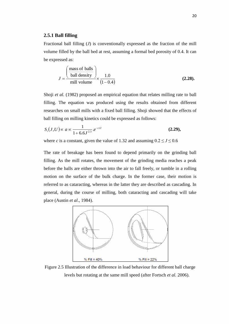
Figure 2.5 Illustration of the difference in load behaviour for different ball charge
levels but rotating at the same mill speed (after Fortsch et al. 2006).
Page 38
21
Fortsch et al. (2006) used Figure 2.5 to describe how the production rate is
affected by an under-loading multiplier which is pronounced by the hole or gap in
the middle of the charge as it is turned by the mill. His team reported that
operating a ball mill at 75 % critical speed and a 22 % charge level creates a
higher cataracting region than at 75 % critical speed and 40 % charge level. They
also observed that cascading action provides the highest grinding efficiency
because of the high total surface area exposed to contact. Finally, Fortsch and his
colleagues argued that as the ball filling is increased, the breakage rate initially
rises to a maximum and then decreases. This is on account of a widely held belief
that as the mill draws maximum power, the rate of breakage also gets to
maximum. That is why in practice, ball fillings usually range between 20 and 40
%; however with today’s ball mills, 35 % charge fillings is considered to be ideal.
2.5.2 Mill filling by powder
The fraction of the mill filled by powder (fc) is expressed as the function of the
mill volume filled by the powder bed, using a formal bed porosity of 0.4. This is
calculated by means of Equation 2.30. The fraction of the mill filled by powder
(fc) has to be determined for every mill operation in which a different J is used,
since the mill should not be under- or over-filled. Under-filling the mill leads to
energy wasted in steel-to-steel contacts, which produces little breakage, but
instead, unwanted material wear. Over-filling the mill, on the other hand, leads to
an effect called powder cushioning, which impedes the efficiency of the breakage
action. That is why it is imperative to fill the mill with an appropriate volume of
powder. The fraction fc of the mill to be filled by powder can be calculated as
follows:
6.0
0.1
volumemill
densitypowder
powder of mass
cf (2.30).
A similar definition applies to slurry, provided that density of powder in Equation
2.30 is replaced by an appropriate density of slurry.
Page 39
22
In order to relate powder loading to ball loading, the formal bulk loading of
powder is compared to the formal porosity of the ball bed (Austin et al., 1984).
This way, the notion of powder filling can be introduced, that is, the fraction of
the spaces between the balls, at rest:
J
fU c
4.0 (2.31).
Austin et al. (1984) reported that powder fillings U between 0.6 and 1 will
generally give the most efficient breakage in the mill. They attributed the small
breakage rates obtained with a low powder filling to the little collision spaces
between the balls that would be filled with powder. Austin and his team then
demonstrated an improvement in breakage rates with an increase in powder, but a
drop in breakage rates as the amount of powder filling was raised further. The
explanation they suggested for the list of these findings was the expansion of the
ball-powder bed to give poor ball-ball powder nipping collisions. Katubilwa
(2012) recommended the operation of ball mills with a slurry filling of close to
unity, based on the graphical analysis he had carried out on laboratory batch
results. His conclusions complemented those of Latchireddi and Morrell (2003)
and Tangsathitkulchai (2003), who proposed U = 1 as the way to ensure efficient
milling. Katubilwa (2012) also suggested operating ball mills at high ball fillings
with a slurry filling of unity as the way to guarantee efficient milling if the
objective is to generate as much fine material as possible (that is, particles of less
than 106 µm).
Shoji et al. (1980) used the results of different studies of small mills at fixed ball
filling to propose an empirical equation that relates milling rate to powder filling:
UU eeaUS 8.01.480.2 for 0.3 ≤ U ≤ 2 (2.32).
The investigations done by Shoji et al. (1980 & 1982) of milling rate on dry
milling and those conducted by Tangsathikulchai (2003) on wet milling
demonstrated that ball filling and slurry (or powder) filling affect the milling rate
regardless of whether milling is done dry or wet.
Page 40
23
2.5.3 Critical speed
The critical speed of the mill is the theoretical rotational speed at which balls
centrifuge on the mill case and do not tumble. This is given by:
dDc
2.42rpm , speed Critical (2.33),
where D is the internal mill diameter and d is the maximum ball diameter loaded
into the mill, both expressed in metres.
The rotational speed of the mill is normally specified as a fraction of the critical
speed c. It has effect on the product size distribution and how fast shell liner
wear. Shoji et al. (1982) found that the industrial mill rotational speeds in use
were 70 – 80 % of critical speed for a ball mill with effective lifters. The typical
operational philosophy is to run the mill at the speed at which the trajectories
followed by the balls are such that the descending balls fall on the toe of the
charge and not on the liners. This is attributable to concordant studies that
demonstrated that low speeds give rise to abrasive grinding owing to the
cascading of the balls, which in turn results in finer grinding and increased liner
wear. At higher speeds, cataracting tends to dominate the grinding process,
resulting in coarser end products and reduced liner wear. Further increase of the
mill speed to close to 100 % leads to centrifuging; the media are carried around in
an essentially fixed position against the shell (Wills and Napier-Munn, 2006).
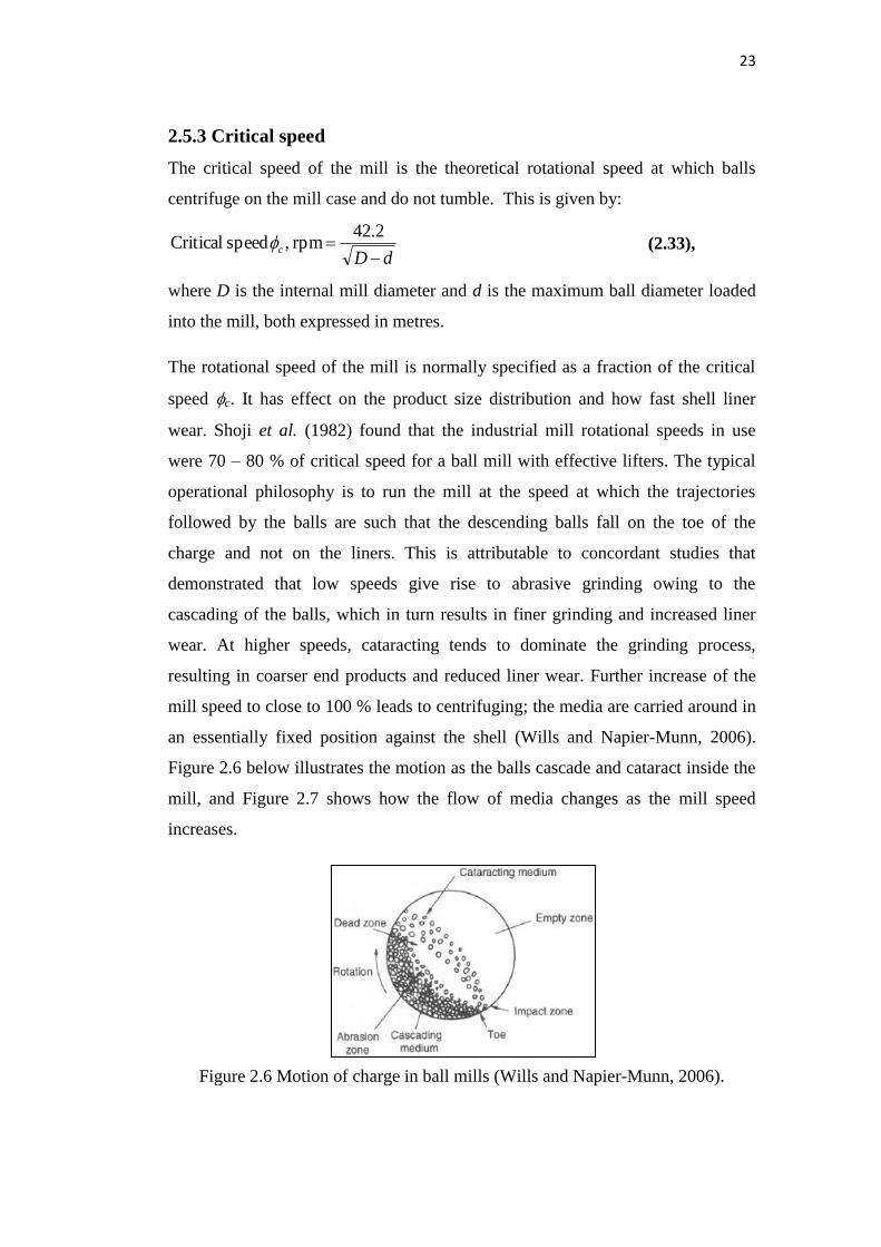
Figure 2.6 below illustrates the motion as the balls cascade and cataract inside the
mill, and Figure 2.7 shows how the flow of media changes as the mill speed
increases.
Figure 2.6 Motion of charge in ball mills (Wills and Napier-Munn, 2006).
Page 41
24
Figure 2.7 Ball mill flow regime as a function of increasing speed
(after Boateng and Barr, 1996).
Austin et al. (1984) showed similarities between the variation of net power with
mill speed and that of specific breakage rates with speed. He proposed an
empirical model that relates the breakage rate of a narrow-sized feed Si to the
fractional speed of the mill, thus giving an indication of the effects of mill speed:
94.07.15exp1
11.0
c
ciS
(2.34),
where is the fraction of the theoretical critical speed Nc of the mill.
This equation is valid only for mill speeds in the range 0.4 < < 0.9.
2.5.4 Ball diameter
A number of published research studies have shown concordance in finding that
fine particles are ground effectively by small balls, because of the increase in the
rate of ball-on-ball contacts per unit time (Austin et al. 1984; Napier-Munn et al.
1996; King, 2001; Katubilwa et al. 2009; Deniz 2012). Also, if a representative
unit volume of the mill is considered, the number of balls in the mill increases, as
1/d3. On the other hand, larger balls have been found to do a better job as far as
the milling of hard ores and coarser feeds is concerned, since high impact energy
is required to break them (Napier-Munn et al., 1996). Katubilwa et al. (2009)
investigated the effect of media sizes on the breakage of coal, and found a
Page 42
25
relatively small variation in breakage for large grinding media sizes, whereas
grinding smaller media sizes increased the yield of fines.
Austin et al. (1984) used their findings from experiments he and his colleagues
carried out on the dry grinding of quartz to show that the specific rate of breakage
decreases as the ball sizes become larger. Small media are at present shunned in
industry because of the cost, yet they offer the desired higher breakage rates.
However, those ball sizes that ensure maximum grinding efficiency ought to be
selected in view of the higher profits to be obtained from a better yield.
An empirical rule that relates the particle size xm to the maximum ball diameter d
has been proposed (Austin et al., 1976 and Napier-Munn et al., 1996) as follows:
xm = K.d2 (2.35),
where K is the maximum breakage factor, reported to be 0.7×10⁻³
for soft to hard
materials by Austin’s group and in the order of 0.44×10⁻³
by Napier-Munn’s
group and xm is equivalent to the particle size at which maximum breakage occurs.
Impact and attrition breakage mechanisms are assumed to predominate above and
below sizes of xm respectively.
In an empirical model that defines the variation in selection function with particle
size (see Equation 2.5), parameter µ is a function of ball diameter. Since
parameters Λ and α are constant for a given material, there is a relationship of
proportionality between and µ. This then implies that µ is a function of ball
size, and gives an indication of the effectiveness of breakage of a given ball size
(Austin et al., 1984). The equation relating the value of xm to µ is as follows:
1
.
mx , on condition that Λ > α (2.36).
Kelsall et al. (1967/68) and Austin et al. (1984) proposed two equations to
express the dependency of the breakage rate on the ball diameter. The set of
correlations are given below:
Page 43
26
d
daa 0
0 . (2.37)
0
0 .d
d (2.38),
where and are the reference breakage parameters corresponding with the
ball diameter d0;
and η are constant exponent factors; and
and are the predicted breakage parameters for ball diameter d.
Figure 2.8 Variation of specific rate of breakage with ball diameter
(Napier-Munn et al. 1996)
The effect of ball size on the selection function can be predicted by combining
Equations 2.36, 2.37 and 2.38 as well as the correction factor in Equation 2.5. An
example of the predictions is illustrated in Figure 2.8.
Austin et al. (1984) presented results which showed Bij parameters (see Equation
2.10) as the function of ball size, taken from the dry grinding of quartz. The
results showed that the parameter γ decreased with an increase in ball diameter of
the media. The authors suggested that this trend was caused by the greater impact
force of collisions involving larger balls, resulting in a higher proportion of fines.
They also suggested that in an abnormal breakage, the value of γ decreases as the
ball sizes increase for larger sizes to the right side of the maximum in S-values,
and attribute it to the mean breakage action in this region caused by the chipping
and abrasion of bigger components, leading to a relatively greater amount of fine
material.
Page 44
27
The breakage function parameter γ is an indication of the relative amount of fines
produced from the breakage of the top size material, and relates to the efficiency
of grinding. Higher γ means grinding is taking place at a slow rate and lower
values indicate more effective breakage action with a high production of fines.
Parameter depends on the material used, and is the fraction of fines produced in
a single fracture. Thus the lower specific rate of breakage found with larger balls
is partially compensated for by the production of a higher proportion of fine
fragments.
2.6 Axial flow through a ball mill
2.6.1 Residence time distribution
A continuous ball mill can be seen as a tubular reactor. One end of the tube is the
inlet for the feed, while the other is the outlet through which the product is
discharged. Depending on the feed flow-rate, the material in the mill may stay
there for a longer period, undergo more breakage and hence come out finer.
Alternatively, the material may flow quickly through the mill and not reach the
degree of fineness required. It appears that the residence time (also called
retention time) of particles is important for the characterization of continuous
milling.
The residence time distribution (RTD) concept, first mooted by MacMullin and
Weber in 1935 (Fogler, 1992), was then presented in a more definitive form by
Dankwerts (1953) and further developed by other researchers (Austin et al., 1983;
King, 2001; van Nierop and Moys, 2002) to model the RTD of rotary mills. A
brief explanation of RTD is a probability distribution function that describes the
amount of time particles spends in the mill. It has proved an indispensable tool for
charting the transport of material over a wide range of engineering processes.
Tracer response and salt tests are the RTD methods most commonly used. When a
tracer is injected into the feed stream to the mill over a very short period, it is
possible to monitor the concentration of traced material at the mill discharge
outlet. While some particles may leave the mill almost immediately, others may
Page 45
28
stay for longer. In statistical terms, this is known as a distribution of residence
time. Figure 2.9 illustrates the tracer response of a typical ball mill from which the
RTD can be inferred.
Figure 2.9 Example of tracer response of a full-scale mill: ball filling J = 25 %
and slurry at 67.3 % solids concentration (after Makokha et al., 2011).
The tracer concentration (in kg/m3) is plotted in Figure 2.9 as a function of time
(in minutes). The conversion of Figure 2.9 to an RTD profile is done by
normalizing the graph with respect to the area under the curve. In other words, if
C(t) represents the tracer concentration exiting the mill at time t, the RTD can be
defined as follows (Levenspiel, 1971):
0
.t
dttC
tCt (2.39).
It is also common to represent the RTD as a cumulative plot of the total fraction
of the tracer E(t) that has left the mill, graphed against time t. Symbolically, this is
given by the equation:
t
t
dtttE0
. (2.40).
Page 46
29
Perhaps the most important point to make is that the mean residence time can be
determined from the cumulative RTD plot. It represents the average time spent by
particles inside the belly of the mill:
0
..t
dttt (2.41).
2.6.2 Simplified flow through a ball mill
One of the simplifying assumptions concerning the flow of material through the
mill is to consider particles as behaving on a first-in-first-out basis (that is, the
particles that come in first also leave the mill first). It is therefore logical to say
that all particles spend the same amount of time inside the mill, counted from the
moment at which they enter. There is also no forward or backward mixing as the
material moves along the mill. Such a model of flow is referred to as a plug flow.
It is understood that all traced feed will exit the mill after the mean residence time
. This can be expressed as follows:
t
ttE
for
for
1
0 (2.42),
where E(t) is the cumulative fraction of traced feed that has emerged at time t after
it has been fed into the mill, and is the mean residence time.
At the other extreme is a fully mixed ball mill, which is assumed to mix the traced
material into the bulk of the charge immediately. The RTD of a perfectly mixed
mill is therefore given by:
ttE exp1 (2.43).
The mean residence time is here defined by FW , with W being the mass of
powder material in the mill (also called the hold-up of the mill) and F the feed
rate.
The three models of mill transportation most widely used in the description of the
flow of material through a ball mill are illustrated in Figure 2.10. Note that the
Page 47
30
flow model of a real full-scale mill is intermediary between two extremes: the
plug-flow and the well-mixed distributions.
Figure 2.10 RTDs of a plug-flow, a perfectly mixed and a real ball mill.
2.7 The Attainable Region technique
In 1997, Glasser and Hildebrandt proposed the Attainable Region (AR) as a new
way of analysing reaction systems in chemical engineering. The tool worked well
on the laboratory and pilot scales. Then, appreciating the similarities between
comminution and chemical reactions, Khumalo et al. (2006 – 2008) extended the
AR technique to comminution process studies. Since then, AR analysis has been
successfully used to optimize comminution of different types of ore in the
laboratory. It is a flexible tool used for graphical analysis of data. It overlooks
milling parameters but instead focuses on the fundamental breakage process and
determines the set of all achievable distributions under the process conditions.
This provides the designer with the best pathway to achieving a specific objective
function from the system feed (Khumalo et al., 2006).
Page 48
31
The power of AR lies in its ability to define process targets accurately, which in
turn permits the engineer to measure the actual process efficiency against a
theoretical target. Khumalo et al. (2006) were able to validate their AR
predictions by showing a good fit between their calculations and their
experimental results. They then investigated the theoretical implications of their
basic model for different specific energy inputs (Khumalo et al., 2007), and
successfully used AR analysis to optimize milling circuits that also include
classification of particle sizes (Khumalo et al., 2008). The main focus of the work
done by Khumalo and his colleagues (2006 – 2008) was on achieving a desired
product with an optimal use of energy. Metzger et al. (2009) used the same AR
analysis technique, but applied it to a different parameter – optimizing the total
time of operation. They found that the AR could be used to determine optimal
polices to reduce milling processing time. Katubilwa et al. (2011) also used the
AR to analyse the effect of ball size on milling, based on the experimental data
they had collected from milling coal. They confirmed the generally accepted trend
that grinding balls of small diameter tend to promote the production of fine
particles at a higher rate than can be achieved by large balls.
As has been shown above, a considerable amount of work has been done by
researchers in the Centre of Materials and Process Synthesis (COMPS) at the
University of the Witwatersrand over the last eight years to apply the AR
methodology to comminution processes. The more detailed examples of its use
given below start with the demonstration by Metzger et al. (2009) that from the
grinding of a single charge constituting single size class feed for different grinding
durations, it is possible to generate product size distributions for those grinding
times and to develop grinding profiles for each size class produced. Figure 2.11
below is an illustration of how experimental data can be represented for both
cases. The grinding profiles can then be grouped into mass fractions m1, m2 and
m3, where m1 is termed the feed size class, m2 the middling size class and m3 the
fines size class. The margins of the mass fractions are dependent on the objective
function to be achieved. For example, if we consider m1 to consist of size class 1
and 2, m2 to be made of size class 3 and 5 while size class 6 constitutes m3, we can
clearly define our objective function.
Page 49
32
Figure 2.11 (a) Grinding profiles of all six class sizes versus time. (b) Cumulative
mass fraction versus average particle size (Metzger et al. 2009).
Figure 2.12 Grinding kinetics as plotted for the three size classes m1, m2 and m3
(Katubilwa et al., 2011).
Figure 2.12 illustrates the mass fractions of m1, m2 and m3. If the objective is to
maximize the production of the middling (m2), then from the AR analysis
illustrated here, we can interpret the graph to determine the optimal grinding time.
We can then extend this analysis to compare the discrete maxima of m2 obtained
under different specified operating conditions. An example of different maxima of
m2 obtained with dissimilar media charges (J) at a single speed is illustrated in
Figure 2.13.
Page 50
33
Figure 2.13 Mass fraction of size class two versus number of revolutions
(Metzger et al., 2009).
Figure 2.14 Representation of particle size distributions as a single trajectory in
the AR space (Khumalo et al., 2007).
Now that mass fractions at different grinding times have been clearly explained,
the next step is to present the data in a final AR format. Figure 2.14 shows how
particle size distributions (PSD) can be connected with grinding time. In this plot,
the boundary curve describes the processes used, and can be interpreted in terms
of pieces of equipment (implicitly identifying the equipment required for best
performance). The turning point of the curve isolates an optimum solution when
the objective is to maximize the mass in size class 2 (m2). This solves the
optimization problem, and provides the process control policy needed to achieve
that objective.
0 0.1 0.2 0.3 0.4 0.5 0.6 0.7 0.8 0.9 10
0.05
0.1
0.15
0.2
0.25
0.3
0.35
mass frac. size class 1
mas
s fra
c. s
ize
clas
s 2
0 minutes
0.5 minutes
1 minute
1.5 minutes
2.5 minutes
4 minutes
7 minutes
10 minutes
optimum point A
Page 51
34
2.8 Optimal floatable particle size
Flotation is widely used for physically separating particles that are hydrophilic
and that are hydrophobic. The ability of air bubbles to selectively adhere to
specific hydrophobic mineral surfaces in a mineral/water slurry allows them to be
removed from the slurry phase and recover them in the froth phase.
Figure 2.15 Typical flotation size/recovery curve (Rule and Anyimadu, 2007).
The first detailed study of the effect of particle size on flotation was done by
Gaudin et al. (1931) who found that the best recoveries of lead, zinc and copper
sulphides were obtained for particles with diameters between 10 – 50 µm.
Recovery falls sharply above 100 µm, but only gradually below 20 µm, as shown
in Figure 2.15. Using other mills and laboratory tests, Trahar et al. (1975)
concluded that recovery is best for particles of an intermediate size. Rule and
Anyimadu (2007) showed that with the flotation equipment currently available, 10
µm for PGM ore can float very well. These authors announced that work was in
progress to identify better ways of improving ultra-fine flotation (for particles of
less than 5 µm), but until that has been achieved, engineers will have to control
milling to maximize the production of the intermediate size, with 9 microns as the
lowest allowable size.
Because PGMs require fine grinds to liberate the maximum amount of valuable
components (Rule, 2008), the fine size of the resultant particles (less than 10
Page 52
35
microns) and gangue association poses processing challenges (Cramer, 2001).
Over-grinding leads to a reduction in the amount of platinum group minerals
recovered (Bryson, 2004), and sets a physical constraint on the flotation of fines,
owing to the energy requirements necessary to enable a very small particle to
attach to a bubble.
Decreased recovery in the fines region is attributable to a lower probability of
particle-bubble collision, since viscous and electrostatic forces have a strong
influence on ultrafine particle attachment. The low flotation rates in this region
will largely dictate the total retention time required (which has to be borne in
mind by the designer of the circuit). Particle recovery by water entrainment is also
a factor in the fine size range.
Particles in the intermediate size range are the most readily floated. The relative
position of the highly floatable size range for two minerals with different degrees
of hydrophobicity is a key factor in selective floatation. Lower recovery in the
coarse region may be related to floatation kinetics as a function of particle size
itself, but it is also in this region that the locking of mineral gangue is most
probable (McIvor et al., 1990). McIvor and his co-researchers pointed out that the
relationship between floatation performance and particle size itself can be used as
a basis for both technical and economic analyses of plant performance.
2.9 Power draw in ball mills: The Morrell model
Mill power has attracted a great deal of attention over the past century, since it is
one of the parameters that determine the feasibility of any mineral processing
plant. Interpretation of the load behaviour enabled Hogg and Fuerstenau (1972) as
well as Arbiter and Harris (1982) to propose mill power equations. Moys et al.
(1996) proposed mill power relations based on the torque-arm approach, which
can be used for different shapes of the load. In this approach, the shape of the load
is considered as a rigid circular segment inclined at an angle equal to the dynamic
of repose of the mill load, from which the centre of gravity is determined. The
Page 53
36
torque of the load at the centre of the rotation of the mill is then calculated, which
in turn can be used to determine the mill power.
The torque-arm approach considers the load as locked in a circular segment,
which many other researcher considered a shortcoming. Moys (1990) and
Fuerstenau et al. (1990) proposed semi-phenomenological models in which the
former proposed the division of load into cascading and centrifuging fractions,
while the latter suggested dividing the load into cascading and cataracting
fractions. These models are based on a mechanistic description of the load
behaviour in conjunction with physically meaningful milling parameters that have
been determined through the empirical results of experiments (Wills and Napier-
Munn, 2005).
Morrell (1993) proposed an energy balance approach which enabled him to
develop a power model based on the motion of the charge. This model proved
superior to the earlier empirical models. He formulated the power draft of the mill
as given by:
S
T
m
i
drNdrgLP r
r
r
net
.cos...2 2 (2.44),
where ri is the inner radius;
rm is the mill radius;
S is the shoulder angle in radians;
T is the toe angle in radians;
Nr, is the angular speed of upward- and downward-moving balls;
L is the length of the mill; and
is the bulk density of charge.
Integrating Equation (2.44) to find a mathematical expression of the net power
while considering the crescent shape and velocity of the load, Morrell (1993)
came up with the following power model, which is applicable to both grate and
overflow discharge mills:
Page 54
37
444
3
323
1
sinsinsinsin 23323
zrzrrzrr
rNL
zrrzrrzrr
rgLNP
iim
im
mmc
TOTpTSciimm
im
mmnet
(2.45),
where p is the density of the slurry;
c is the average density of the grinding charge;
TO is the slurry toe angle for overflow discharge mills, which will be
equal to T for grate discharge mills;
rm is the internal radius of the mill;
ri is inner surface radius charge, which marks the boundary between the
active part of the charge and the inactive kidney-shaped media charge;
z.ri (the product) is the normalised radial position corresponding to the first
inner concentric layer of the charge which is entrained by the mill,
determined from photographs of the mill charge in motion. The z
parameter was found to be a function of the fractional mill filling Jt.
The definition of z is established in such a way that as Jt increases, z
tends to zero and hence the rotational speed at any radial position r, that
is, Nr tends to Nm;
Nm is the rotational speed of the mill in revolutions per second;
L is the length of the mill; and
g is the constant of gravity.
The Morrell model is adequate, especially for ball mills, which are operated at
speeds where there is no centrifuging.
2.10 Net power draw and milling efficiency
Austin et al. (1984) presented a typical variation of the net power required to turn
the mill with rotational speed. The results showed that the work input to the mill
increases linearly with the rotational speed to a point at which the maximum
power draw is reached. A further increase in rotational speed leads to a reduction
in power, as the mill starts to centrifuge. The maximum power is usually found in
Page 55
38
the range of 70 – 80 % of critical speed (Wills and Napier-Munn, 2005), or 70 –
75 % for mills of large diameter with a full ball loading (J ≈ 40 %) (Austin et al.,
1984). This made it possible for engineers to use speed to modify mill power,
especially in the case of dry grinding, where the effect of powder filling is
insignificant. For wet milling, Tangsathitkulchai (2003) showed that mill power
rises steadily with an increase in slurry filling, and reaches a maximum at a slurry
filling of approximately 1.0 before starting to decline. Katubilwa (2012) used
kinetic milling profiles (AR graphs that show the evolution of mass fraction in
each class in relation to the energy consumed) to investigate the effect of powder
filling on mill power. He found that a powder filling of U = 1.5 achieved the
maximum desired size class (-75 +9 m) at a lower energy input than U = 3.0.
Metzger (2011) used the AR to investigate the effect of media size on energy, and
showed that smaller media require much more energy while producing a smaller
amount of product in the desired size class. He recommended the use of larger
media under optimal conditions for industries where energy saving is a primary
concern. He also showed that less energy is used when operating on larger
amounts of grinding media (higher J) than smaller amounts, although it does not
obtain as much of the desired product as when the combination of larger grinding
media, at the slowest rotation and lower J, is used.
2.11 Classical configuration of milling circuits
Milling circuits play an important role in achieving desired product size
distributions and product properties since it has a direct link to the energy
consumption of the whole process. The production chain can be made up of
grinding mills connected to classifiers. The way in which the grinding mills and
classifiers are connected determine the type of a circuit they form. There are
generally four single stage circuits (Austin et al., 1984) used in practice:
Grinding circuits employing mill in an open circuit
Normal closed circuit
Reverse closed circuit
The combined closed circuit
Page 56
39
Figure 2.16 is an illustration of a combined closed circuit in which all the circuit
feed material is subjected to the classification action before entering the mill. The
course product from the pre-classifier is the actual make up feed G to the mill.
The undersize by-passes the mill and flows into the circuit product. The makeup
feed G is milled and flows out of the mill as the mill product and subjected to the
second classification in the post-classifier. The coarse particles from the post-
classifier is fed back to the mill and is mixed with feed G before being subjected
to the milling action again, while the undersize size product flows into the circuit
product stream (Austin et al., 1984).
Figure 2.16 The combined closed circuit (from Austin et al., 1984).
Depending on the presence of the first classifier, the second, or both as well as
their corresponding loops (streams), the combined circuit can reduce to an open, a
normal closed, or a reverse closed circuit. In the case of an open circuit, the mill is
operated without being directly influenced by a classifier. The normal closed
circuit does not have the first classifier and therefore the make-up feed G is the
actual feed stream. Conversely, the reverse closed circuit keeps only the first
classifier. There are advantages and disadvantages associated with each specific
configuration. Suffice it to say that the general motivation is to optimise the
production of material of a specified fineness of a grinding mill hence the desire
to limit this study to an open circuit.
Page 57
40
2.12 Summary
In this chapter, the mathematical models that best describe the breakage process in
mills were reviewed. Because of its simplicity and flexibility, the population
balance model is applied in most comminution processes and is the preferred
method for our investigations. The model is based on defining two fundamental
concepts: the selection function and the breakage function. The empirical
description of the two concepts has shown that four selection function parameters
and three breakage function parameters are required to predict mill product size
distribution, which in turn can be used to set the operating conditions of the mill
as well as the objective function to be optimized.
The attainable region, which complements the analysis of milling by the PBM
framework as a graphical technique, was also reviewed in this chapter. The
success of subsequent research work applying AR methods to comminution has
shown that the AR is a novel analysis technique that can be used to optimise
laboratory scale milling. However, it is generally believed that at this stage, the
AR technique is not sufficiently robust to be applied to industrial milling.
It was also apparent from the background information given that the milling of
PGM ore to achieve the product size which ensures maximum recovery during
flotation is a challenge. This makes further study of the situation difficult since
competition among the various processing industries has severely restricted the
amount of scientific information concerning PGM available. As a contribution
towards alleviating this problem, information is provided in this thesis that can be
used for simulation and optimization purposes, which in turn will lead to further
development in the milling of PGM ores. Greater recognition of the AR technique
as the tool of choice in the analysis and optimization of mineral processing
circuits is expected to result from this study, which will use the AR and PBM
approaches in a complementary fashion to ascertain the operating conditions
under which a preselected industrial mill will be able to optimize product size
distribution for flotation purposes.
Page 58
41
Chapter 3 Experimental programme, equipment and
simulation strategies used
3.1 Introduction
In this chapter, the experimental methods and simulations used to fulfil the
objectives of this investigation are set out. The information provided comprises a
description of the laboratory mill used for batch testing, the experimental
conditions, and, after that, the details of the experimental design, the materials
used and the procedures followed.
The experimental programme consisted of feed sample and ball size preparation,
batch grinding tests and particle size analysis. All of the milling runs were
performed in a dry environment.
3.2 Experimental equipment and programme
3.2.1 Description of the laboratory grinding mill
During the first part of the experimentation, the milling kinetics of PGM ore were
examined in order to determine the breakage and selection function parameters
that would later be used for modelling purposes. All the batch grinding tests on
the ore were carried out on a laboratory scale batch mill in the Department of
Chemical Engineering at the University of the Witwatersrand. Figure 3.1 is a
photograph of the mill set-up.
Page 59
42
Figure 3.1 View of the laboratory ball mill.
The laboratory batch mill is installed on a steel structure that also carries all the
control and measurement facilities required to run the mill. Manipulation of the
mill speed is achieved through an electronic speed meter that enables one to set
and control the motor speed. The power of the mill can be measured through a
load beam that converts the force exerted onto it into the corresponding voltage.
One of the ends of the load beam is attached to a piece of rod which generates a
force attributable to the rotational torque of the mill. The mill is fitted with eight
symmetrically-spaced lifters (see Figure 3.2), and is driven by a variable speed
motor. The internal dimensions of the mill are given in Table 3.1, along with the
test conditions.
Figure 3.2 Picture of the laboratory grinding mill used for the experiments.
Page 60
43
Table 3.1 Specifications of the mill
Mill dimensions Diameter
Length
Volume
0.302 m
0.282 m
19.493 litres
Liner configuration Number
Dimensions
8
0.013 m height
0.025 m width
0.272 m length
Test conditions Ball filling, JT
Powder filling, UT
Mill filling, fc
Mill speed, cT
20 %
0.75
0.06
75 % of critical speed
J =
×
fc =
×
U =
The latter are classically defined as follows. The ball filling (J) is conventionally
expressed as the fraction of the mill volume filled with grinding balls at rest while
assuming an average bed porosity of 0.4. The mill filling (fc) is represented as the
fraction of the mill volume filled by the powder bed, using a formal bed porosity
of 0.4. The powder filling (U) is the fraction of the spaces between the balls at
rest that is filled with powder. These definitions and the corresponding formulas,
which are shown below in Table 3.1, were used to make the calculations
necessary before the laboratory tests could be carried out.
3.2.2 Laboratory testing protocol
The experimental programme to investigate the millings kinetics of PGM ore was
conducted using a combination of mono-sized balls and narrow-sized feed sizes,
as shown in Table 3.2. Dry milling was done in all the experimental tests, which
were carried out with a ball filling of JT = 20 %, a powder filling of UT = 0.75, and
a mill speed cT = 75 % of critical speed.
Page 61
44
Table 3.2 Experimental design
Feed size in m Ball diameter dT
Upper size Lower size 10 mm 20 mm 30 mm
850 600 x x x
600 425 x x x
425 300 x x x
3.3 Feed material preparation
The platinum ore used in this work was obtained from the feed to the secondary
mill of the Anglo Platinum Waterval mine in the Republic of South Africa. The
mine’s internal reports indicate that the ore has a density of 3.47 g/cm3. The
platinum ore was collected in batches of 10 kg bags and was split using a Jones
riffler in order to obtain a representative sample for use. The individual samples
generated from that exercise were then mixed to a large feed sample
After collecting the feed sample, the moisture content was determined by drying a
500 g sample of the platinum ore at 50˚C in an oven overnight. When the
difference in weight before and after drying was measured, the moisture content
was found to be 1 %.
The next step was to prepare narrow-sized feed samples for batch testing: -850
+600 µm; -600 +425 µm and -425 +300 µm from the -1200 µm sample that was
received. Following this, three sizes of grinding media were prepared: 10 mm, 20
mm and 30 mm in diameter. In each case, the mass of the grinding charge was
fixed at 17840 g which represents a ball filling JT of 20 %. A series of batch
milling tests were then carried out under different conditions, in order to
characterize the breakage properties of the platinum ore fully. More detailed
description of the experiments is covered in the following sections.
3.3.1 Feed preparation
The specifications of the mill given in Table 3.1 were used to determine the
amount of material needed per test. It was found that a feed sample of 2.771 kg
for a density of 3.47 g/cm3 was required for all the tests. This mass of powder was
Page 62
45
calculated for a fractional interstitial filling UT = 0.75 and a load porosity ƐL = 0.4,
which led to the determination that a mass of 17 840 g of steel grinding media and
2 771 g of ore would be loaded per run. The mill speed was set at 75 % of critical
speed. (The theoretical critical speed was approximately 59.7 rpm.)
Three narrow-sized feeds were prepared from the feed material with particle size
range from below 25 µm to 2000 µm in the following classes (-850 +600 µm, -
600 +425 µm and -425 +300 µm). For each size class, 15 kg of material was
initially prepared. Then, 2 kg from every 15 kg platinum ore batch was sieved for
50 min in order to ensure that each mono-size feed contained uncontaminated
particles within its size class. The above screening time of 50 min was established
by sieving 500 g of the platinum ore for 60 min, and stopping at 10-minute
intervals to determine the changes in mass retained on the screens of interest. As
shown in Table 3.3, the screening time, that is, the time at which the mass stopped
changing, was found to be 50 min.
Table 3.3 Mass retained on each sieve at different times
Size Sieving Time (min)
10 20 30 40 50 60
850 µm 46 g 44 g 43 g 43 g 42 g 42 g
600 µm 47 g 46 g 46 g 46 g 46 g 46 g
425 µm 87 g 86 g 86 g 85 g 85 g 85 g
300 µm 75 g 75 g 75 g 75 g 75 g 75 g
pan 246 g 249 g 250 g 251 g 252 g 252 g
Fractions of the platinum ore retained on the screens of interest were stored in
appropriately labelled plastic bags. Finally, three samples from each batch of
narrow-sized feed material were prepared by splitting the ore using a Jones riffler
to make 2 771 g representative feed platinum ore samples ready for batch tests. In
total, nine feed samples were prepared; for experiments involving three media
sizes as shown in Table 3.2.
Page 63
46
3.3.2 Preparation of the grinding balls
The breakage characteristics of the platinum ore were determined using the single
ball sizes listed in Table 3.4, which also gives the number and sizes of the balls.
Mono-sized grinding media were prepared by sorting the spherical steel balls to
predefined size intervals in order to make up the desired quantity.
Table 3.4 Mono-size media charges used
Ball size dT Number of balls Total mass (kg)
10 mm 4 441 17. 8
20 mm 510 17. 8
30 mm 150 17. 8
3.3.3 The batch grinding tests
The experiments were performed in batch mode, using a one-size fraction method
(Austin et al., 1984). The feed material was ground for a total of 30 min in all
tests. Per batch run, the grinding was interrupted at 0.5, 1, 2, 4, 8, 15 and
eventually 30 min intervals. After each interruption, a full-size distribution of the
mill product was measured and the material was re-introduced into the mill after
the sample was analysed.
Before each batch test, a blank sieving test was carried out on the prepared feed
material, after which he loaded the sample to be milled into the mill with media of
the appropriate size and weight. The mill was then run and the material milled for
30 seconds and stopped in order to do particle size analysis. The mill powder was
offloaded, then split, so as to obtain a representative sample of the mill content.
The ground product was removed, then by appropriate sampling technique (using
a splitter) a representative sample of the mill content was obtained for sieve
analysis.
The representative sample was later used for size analysis after the laboratory
procedure described in the next section had been completed. After size analysis,
the fractions retained on the sieves were weighed. The fractions were recombined
and added back to the mill with rest of the unscreened sample for the next milling
Page 64
47
interval. This procedure was repeated until the grinding routine mentioned above
was completed.
3.3.4 Particle size analysis
A complete size analysis of a sample of platinum ore collected from the mill was
carried out using a nest of sieves arranged according to screen sequence with
the top sieve being 850 µm. The following sieves were used: 850, 600, 425, 300,
212, 150, 106, 75, 53, 38 and 25 µm. The minus 25 µm were collected in a bottom
pan.
Before sieving, a test was conducted to determine the optimum screening time
that would enable the material to be screened without the retention of fines on the
coarser sieves (contamination) or over-sieving, which would lead to pre-breakage
of the material before the milling had taken place. Having determined the
optimum sieving time, a 100 g sample of platinum ore from the mill was dry
screened for 50 minutes, and after that, each sieve was weighed to ascertain the
mass of material retained. The sieves were then restacked in order, but without a
pan at the bottom, and wet washed to recover the residue dust on each screen. The
washed through sample was dried in the oven at 50˚C. Then, the dried material
was weighed and the recorded weight added to the -25 m pan fraction.
The process described above for all the grinding experiments were repeated. The
same nest of sieves was used throughout the experiments in the interests of
maintaining consistency. The masses of material on each sieve were added
together, and the total sum was subtracted from the initial mass of the sample
before the wet sieving had taken place. The difference in mass was added to the
mass of materials in the pan to achieve mass balance.
3.3.5 Data collection and processing
Raw data collected from the experiments were used to determine the breakage
function parameters ( , γ, from Equation 2.10) and the selection function
parameter ( from Equation 2.6) by means of the progeny fragment distributions
Page 65
48
from the breakage of the mono-size classes -850 +600 µm; -600 +425 µm and -
425 +300 µm.
3.4 Estimation of the breakage characteristics of the ore
A Matlab®
code was written to execute the population balance model and the
relevant equations discussed in chapter 2 were incorporated in the scheme. All
three breakage function parameters (β, γ and from Equation 2.10) as well as one
selection function parameter (α from Equation 2.6) were the input parameters
determined from the experimental tests. The remaining selection function
parameters (ɑT, Λ and µT from Equation 2.2) were estimated by letting the
simulator search for the best combination of all the parameters that is most
successful in minimizing the sum of squared errors between the predicted and
experimental product size distributions. Once the parameters were determined, it
was possible to predict product size distribution for any given grinding period. A
flow sheet for the scheme is shown in Figure 3.3 below
Figure 3.3 Diagrammatic representation of the simulator used.
The calculation procedure makes use of the Matlab® function “fmincon” which
uses a sequential quadratic programming method. This function basically solves a
quadratic programming sub-problem; an estimate of the Hessian of the
Lagrangian is updated after each iteration by globally converging all the unknown
parameters simultaneously and not adjusting them one at a time.
Once all the selection and breakage functions had been estimated, the milling
evolution of size range (-106 +25 µm) were simulated, and then extrapolated to
300 min. Finally, additional experiments were done by grinding the ore for 60, 90,
Page 66
49
120 and 240 min, to enable a comparison between the simulation results and the
experimental data (refer to Chapter 4).
3.5 Scale-up Methodology
3.5.1 Batch test data
In the previous section, the breakage function and selection function parameters
were measured and estimated from laboratory batch experiments. This section
describes how these parameters were extended to full-scale milling.
Before that, the reader of this dissertation is asked to recall that the batch tests
were done in a laboratory scale ball mill with an internal diameter (DT) of 0.30 m,
and a length (LT) of 0.28 m. The mill was fitted with eight lifters, the dimensions
of which are a height of 13 mm, a width of 25 mm and a length of 272 mm.
Mono-sized balls and narrow-feed size classes were used in each test. The media
sizes (dT) considered were 10 mm, 20 mm and 30 mm steel balls and the feed size
classes used were (-850 +600 µm, -600 +425 µm and -425 +300 µm) of the PGM
ore. The test conditions were as follows: ball filling JT = 20 %, slurry filling UT =
0.75 and the mill speed cT = 75% of critical speed. All breakage function
parameters (, γ and ) and the selection function parameter (α, aT, Λ and µT)
were based on the laboratory batch mill tests.
3.5.2 The industrial mill
The specific rates of breakage obtained from the test conditions in the laboratory
mill were converted to the operating conditions of a typical industrial mill by
means of a methodology recommended by Austin et al. (1984). An open circuit
mill which had already been comprehensively studied and characterised by
Makokha et al. (2011) was the source of industrial data used for the research work
described here. The mill was a secondary grinding unit of the UG2 Platinum
Waterval concentrator situated in Rustenburg, in the North West province of the
Republic of South Africa. It has an overflow discharge design with an inside
Page 67
50
diameter (D) of 7.312 m and length (L) of 9.6 m, and is run in an open circuit. It is
fitted with 44 rubber lifter bars 100 mm high, and is loaded with forged chromium
steel balls 40 mm in diameter (d). The wet overflow mill processes fine (less than
1 mm) platinum feeds, grinding the material to less than 106 µm to meet flotation
requirements. However, slimes (that is, material less than 10 µm in size) have to
be avoided, because they may compromise the flotation process.
For the purpose of scaling-up and modelling, the mill was initially assumed to
behave as a plug flow reactor. Consequently, the grinding time was regarded as
the mean residence time of the mill (Austin et al., 1984).
3.5.3 The scale-up procedure
The scale-up methodology proposed by Austin et al. (1984) is applicable only to
materials the breakage and selection function parameters of which have been
determined in the laboratory. In this study, the breakage properties of the platinum
ore that had already been established were applied, a decision reinforced by the
knowledge that these breakage properties had been measured on a feed sample
similar to that of the industrial mill under consideration.
On that basis, a Matlab® script was written to scale up the selection function
parameters from the laboratory test conditions to the industrial mill. The ore was
assumed to be normalisable, so that the breakage function remained unchanged.
The initial input parameters were those for the selection functions (α, aT, µT and
Λ) obtained in the laboratory. Other inputs to the Matlab® code were the grinding
conditions pertaining to the batch mill (DT, JT, UT, cT, dT) and to the simulated
industrial mill (D, J, U, c and d). For a given set of user-defined industrial mill
conditions, specific rates of breakage for the industrial mill were predicted using
Equations (2.20 – 2.25). Once the scaled-up selection function values had been
determined, they were incorporated into the population balance model (Equation
2.11) together with the laboratory breakage function parameters. Then product
size distributions were generated for different grinding times (also termed mean
residence times in a continuous milling setup). Finally, the milling kinetics of the
Page 68
51
desired size class (-106 +9 µm) were deduced from the particle size distributions
generated for each set of industrial mill conditions under consideration. The
effects of each milling factor on the production rate of the desired size class were
then explored.
3. 6 Simulation of the residence time
The aim of determining the optimal residence time is to extend the use of the AR
technique from batch to continuous milling. However, the scope of the work
described in this thesis was limited to the optimisation of the residence time of
particles inside the mill. The circuit was treated as an open circuit which was
assumed to operate without being directly influenced by a classifier. To fulfil this
purpose, a full characterization of both the full-scale mill used for the study and
the ore that was being processed had already been given. This provided the
material to initiate a simulation programme for the large mill in order to generate
data for AR analysis. Initially, the residence time was optimised using the plug
flow and perfectly mixed transportation models. This was later carried on to the
next stage, using residence time distribution (RTD) transport model which
comprises, first, a dead zone, followed in sequence by models of a large fully
mixed reactor and two smaller but equally fully mixed reactors, as shown in
Figure 3.4. The choice of this transport model has been motivated by the fact that
the parameters of the model were previously determined for the industrial mill
used in this research by Makokha (2011).
Figure 3.4 Schematic representation of the tanks in series model with dead time.
(after Makokha et al.,2011)
Page 69
52
As far as the properties of the ore are concerned, the breakage and selection
function parameters measured in the laboratory were used to characterise the
material. These parameters were measured by means of batch tests using the one-
size-fraction method described by Austin et al. (1984). The parameters correspond
to the following experimental conditions: feed size (-850 +600 µm); ball diameter
dT = 20 mm; ball filling JT = 20 %; powder filling UT = 0.75; mill speed cT = 75
% of critical; and mill diameter DT = 302 mm.
As for the full-scale mill in question, it is an overflow discharge mill, run in open
circuit and used in the secondary grinding of UG2 platinum ore. Its technological
and operating specifications are as follows: mill power draw is about 9500 kW at
30% mill filling; mill full length L = 9.6 m; mill diameter D = 7.312 m inside
liners; mill speed c = 75 % of critical; ball filling J ranging from 25 to 33 %;
steel ball diameter d = 40 mm. The mill is lined with 44 rubber lifters which have
a height of 100 mm. The solids concentration in the slurry is on average 75 % by
mass for a 330 tons per hour throughput.
It is important to emphasise that the choice of this industrial mill was motivated
by the fact that RTD and milling kinetics have already been comprehensively
studied (Makokha, 2011; Makokha et al., 2011). In addition, sufficient data are
available for validation purposes.
A Matlab® script for the simulation programme that was based on the solutions of
the PBM applied to continuous milling was written. The PBM parameters
obtained from laboratory experiments on the same material were scaled up to an
industrial mill using Equations 2.20 – 2.25. Next, the PSD of the full-scale mill
were generated using Equations 2.12 – 2.19, and finally an AR optimisation
routine ran to determine the optimum residence time for both the fully-mixed and
the plug-flow mills and the residence time distribution mill models.
Page 70
53
3.7 Simulation of the power draw
The Morrell model was used for predicting the net power drawn by the full-scale
mill. The Matlab® script written to calculate the net power (PNET) incorporated a set
of operational conditions which included mill speed, ball and slurry fillings.
To satisfy the requirements of the Morrell model, the charge density was
calculated first, and then the toe angle and the shoulder angle. After that, in-mill
parameters such as the charge inner surface radius were worked out before
Equation (2.45) could be applied to obtain the net power draw.
3.8 Summary
All the experimental tests were completed using the equipment and techniques
described in this chapter. The results of experiments carried out on the Wits
laboratory mill, coupled with the back-calculation technique, enabled the
determination of the milling parameters of the platinum group minerals ore
needed for modelling purposes.
The selection function parameters obtained were used in empirical models to
convert specific rates of breakage from the laboratory test conditions to a
preselected overflow full-scale ball mill. Data relating to the effects of operational
factors such as the mill filling, mill rotational speed, grinding media filling and
media size were generated and analysed. In addition, reported data from the same
full scale mill were used and compared with those generated using the models.
The effects of the operational factors as well as the residence time and net power
draw were simulated with the aim of optimizing the product size distribution for
flotation purposes.
Page 71
54
Chapter 4 Determination of the milling parameters of a
Platinum Group Minerals ore to optimize
product size distribution for flotation purposes
The results of this chapter have been published in the Minerals Engineering
Journal under the reference: Chimwani, N., Glasser, D., Hildebrandt, D.,
Metzger, M.J., Mulenga, F.K., 2012. Determination of the milling parameters of a
platinum group minerals ore to optimize product size distribution for flotation
purposes. Minerals Engineering, vol. 43 – 44, pp. 67 – 78
This is completely my work, i did all the experiments and processing of data as
well as writing the paper, the other authors are my supervisor except M.J.
Metzger whose contribution was in helping me to structure the paper into a
journal format.
Abstract
Most concentrators desire to operate under optimal design configuration that
guarantees high mineral recovery and low operational costs. The optimal milling
conditions can be determined by studying the material to be milled on a laboratory
scale under standard conditions that make it possible for the selection and
breakage function parameters to be measured. These parameters provide the basis
for the mathematical simulation of grinding for optimisation purposes.
Accordingly, three narrow-sized feeds (-850 +600 µm, -600 +425 µm and -425
+300 µm) of a platinum ore were milled, using three different ball sizes (10, 20
and 30 mm), in a laboratory mill for a range of grinding periods (0.5, 1, 2, 4, 8, 15
and 30 min). The data collected were used to determine the breakage function
parameters and some of the selection function parameters. The remaining
parameters were back-calculated within the population balance model framework.
The parameters were then used to obtain the product size distribution, which was
later compared with those determined from the experimentally measured data. The
milling kinetics for the desired size class (-150 +25 µm) for grinding times
ranging between 60 – 240 min were also measured and compared with the
extrapolated simulation.
Page 72
55
A good match was found between the predicted and measured size distributions.
The results of the milling done for 60, 90, 120 and 240 min grinds to validate the
simulation model estimates were also satisfactory. This further confirmed the
validity of the determined parameters. The measured selection and breakage
function parameters then provided the foundation on which the determination of
the grinding conditions for optimal flotation was built.
Page 73
56
4.1 Introduction
In PGM recovery, the primary reason for milling materials to smaller particles is
to liberate the valuable components dispersed in the host matrix. When the
material has been reduced to a size small enough to give sufficient liberation of
the valuable components, these components are separated from the host matrix by
downstream processes such as flotation. The size reduction operations, especially
the final stage of grinding before the separation circuit, constitute the primary feed
preparation for the separation circuit (Coleman, 1983).
Liberating PGMs, especially those present in the Upper Group 2 Reef (UG2) from
their host matrix, which consists of base metal sulfides, silicates and chromites
poses processing challenges (Hay and Roy, 2010). Most of them are attributable
to the fineness and gangue association of the PGMs (Cramer, 2001). The valuable
minerals in UG2 have significantly smaller average grain sizes and require fine
grinds to optimally liberate the valuable components (Rule, 2008). Cramer (2001)
anticipated the future of the PGM processing industries would require further
development of the processes to address the encountered technical challenges.
This confirms that the design and performance of the PGM processing circuits is
poorly understood, and hence a topic of interest (Bryson, 2004). Optimizing the
milling stage is one way of improving the efficiency of the PGM processing
circuits.
In order to optimize the milling stage, requirements of the flotation in terms of
particle size have to be fully understood first, since either over-grinding or low
liberation leads to the reduction in the amount of PGM recovered (Bryson 2004;
Rule and Anyimadu, 2007). This would be followed by understanding the
breakage properties of the ore to be used which is modelled by the selection and
breakage function parameters as discussed in chapter 2.
These parameters are used to predict the product size distribution, which in turn
can be applied in setting the standard operating procedure of the mill. Discrete
size classes are usually used, for they provide adequate approximations for
practical computation (King, 2001). The parameters describe the breakage and
Page 74
57
characterize the objective function that is to be optimized. Examples of objective
functions could be to minimize the total energy consumption in a circuit, achieve
a specified particle size distribution (PSD), or to shorten the total duration of
operation.
The work reported in this chapter helps the engineer to determine the preliminary
parameters describing the milling behaviour of PGM ore. This is necessary
because the PGM ore processing industries have been unwilling to divulge
scientific information concerning their ores, for fear of competition.
The research therefore seeks to provide information that can be used for
simulation and optimization purpose which leads to further development of the
milling process of PGM ores.
4.2 Results and discussions
The experimental work discussed in chapter 3 is analysed to obtain the breakage
parameters that characterise the PGM ore.
4.2.1 Determination of the selection function parameters
The rate of breakage for PGM ores was obtained numerically using Equation 2.4
as the mean value of the effective selection function. Figure 4.1 shows the
experimental results obtained from plotting the mass percentage retained on the
top screen against grinding time t on a log–linear scale for the feed size -600 +425
µm using three different media sizes, 10 mm in Figure 4.1(a), 20 mm in Figure
4.1(b) and 30 mm in Figure 4.1(c). The graphs do not start at 100 % indicating
that the initial sample had undersize material. This indicates that the equations are
different from the first order model (Equation 2.2) and therefore, the breakage in
the mill has departed from the first-order hypothesis. That is why Equation (2.4)
was used to determine the selection function for feed sizes -850 +600 µm, -600
+425 µm and -425 +300 µm when milled with different media sizes.
Page 75
58
(a) (b)
(c)
Figure 4.1 First-order plot for UG2 ore mono-size class (-600 +425 µm) ground
with different media sizes (dT): (a) 10 mm; (b) 20 mm; (c) 30 mm.
The results presented in Table 4.1 show that for the ore feed sizes -425 +300 µm
and -600 +425 µm, the magnitude of the selection function is inversely
proportional to the ball size. This is because, if the balls of smaller diameter are
used for the same JT to grind relatively small particles, the rate of ball-on-ball
contacts per unit time increases. This results in a higher rate of breakage of
smaller particle sizes by balls of smaller diameter (Austin et al., 1984). A different
trend can be observed if a feed size with bigger particles is used. Austin et al.
(1984) was able to show that as the diameter of the ball increases, the mill can
break a feed containing larger size of particles more efficiently. This is confirmed
by the selection function of feed size -850 +650 µm, which rises with an increase
in ball diameter, as shown in Table 4.1.
y = 69.236e-0.123x
1
10
100
0 10 20 30
mi(t
)/m
i(0)
Grinding Time (minutes)
y = 78.271e-0.171x
0.1
1
10
100
0 10 20 30
mi(t
)/m
i(0)
Grinding Time (minutes)
y = 92.895e-0.175x
0.1
1
10
100
0 5 10 15 20 25 30
mi(t
)/m
i(0)
Grinding Time (minutes)
Page 76
59
Table 4.1 Selection functions for different feed sizes and media sizes
Mono-sized UG2
materials
Media size (mm)
10 mm 20 mm 30 mm
-850+600 µm (S1) 0.18 0.28 0.29
-600+425 µm (S2) 0.21 0.20 0.18
-425+300 µm (S3) 0.16 0.13 0.11
The selection function values in Table 4.1 were plotted against particle size, as
shown in Figure 4.2. It can be seen that the increase in selection function with an
increase in particle size is linear and almost linear for 30 mm balls and 20 mm
balls respectively. The figure also shows that the maximum value of the selection
function for the 10 mm balls has been reached, and that the breakage rate
decreases with a further increase in particle size beyond 600 μm. The size classes
-850 +600 µm and -600 +425 µm are too big and strong to be properly nipped and
fractured by the 10 mm balls, hence the drop in the rate of breakage, which is in
agreement with Austin et al. (1984).
In Figure 4.2(a), the parameter α was determined by the 30 mm ball curve using a
power function. The 30 mm curve was chosen because it is considered to be in the
linear region, that is, before the xm (the size at which the maximum value of S
occurs). The value obtained for α is 1.40. Figure 4.2(b) shows what a complete
selection function curve should look like (King, 2001). The part of the curve that
shows normal breakage behaviour is the region where S has not passed through
the maximum, and abnormal breakage behaviour is shown by the region where S
has passed the maximum. When one compares Figure 4.2(a) and 4.2(b), one can
see that Figure 4.2(a) represents only a small portion of the entire curve of the
selection function. It follows that it would be unwise to assume that it provides a
basis for the accurate determination of all parameters associated with the selection
function. However, the value of α (the slope of the linear portion of the curve)
can be determined from the 30 mm curve in Figure 4.2(a), and this value was fed
into the population balance model for simulation purposes.
Page 77
60
Figure 4.2 (a) Variation of S with particle size. (b) Graphical procedure for the
determination of the parameters
(Austin et al. 1984).
4.2.2 Determination of the breakage function parameters
Figure 4.3 shows the primary breakage distribution plots of all the feed size
classes for 10 mm, 20 mm and 30 mm media sizes, which were determined using
Equation 2.9 (B-II method). Austin et al. (1984) recommended that shorter
grinding times, which result in 20 – 30 % broken materials out of the top size,
should be used in this procedure. Although shorter grinding times give
researchers the most accurate estimates of the breakage function, Austin and
Luckie (1971) showed that even with 65 % broken material, the procedure
remains sufficiently accurate to be used.
0.1
1
0.1 1
Spe
cifi
c ra
te o
f b
reak
age
Si
min
ute
s-1
Size (mm)
10 mm
20mm
30mm
Page 78
61
Figure 4.3 Variation of breakage function values with feed size.
The breakage function data obtained were fitted to the empirical model in
Equation 2.10 and the breakage function parameters for PGM ore were evaluated.
The average breakage function parameters determined for all feed size classes and
media sizes used were found to be: β = 6.2, γ = 1.30 and = 0.59. These
parameters were then fixed for the rest of the simulations as the breakage function
is considered to be independent of milling conditions.
These parameters are close to those obtained by Yekeler (2007) for chromite,
which were as follows: β = 7.9, γ = 1.14 and = 0.75. Austin et al. (1984) also
found values of β = 5.8, γ = 1.30 and = 0.58 for the experiments they conducted
on quartz. Though these ores are not identical, the similarity in the results
provides confidence in the parameter determination method. Most important of
all, the PGM ore was considered to be normalizable, since no specific trend was
identified in Figure 4.3.
0.01
0.1
1
0.1 1
Cu
mu
lati
ve B
reak
age
Par
ame
ter
Bi,
j
Relative Size xi/xj
(850-600)10mm
(850-600)20mm
(850-600)30mm
(600-425)10mm
(600-425)20mm
(600-425)30mm
(425-300)10mm
(425-30)20mm
(425-300)30mm
Average
Page 79
62
4.2.3 Particle size distributions (PSD)
The parameters of the selection and breakage function evaluated from the
experimental data were used as initial estimates for the model in the parameter
search process. The parameters (ɑT, Λ, γ and µT) were estimated by the
optimization model, which searches for the best combination of these parameters
that performs best at minimizing the residual error between the experimental and
the predicted product size distributions. Table 4.2 shows the predicted breakage
and selection function parameters for all feed sizes using 10 mm ball diameters,
which in combination yielded the best fit between predicted and experimental
product size distributions. It can be seen that the value of ɑT decreased with an
increase in feed size. The possible explanation for this behaviour is that the rates
of breakage of smaller sizes are higher with balls of smaller diameter, and that the
S values of feed sizes comprising larger particles will be to the right of the
maximum, giving lower rates of breakage (Austin et al., 1984). This was also
confirmed by the results given in Table 4.1, which show the drop in S values for
10 mm balls as the feed size increases from 600 to 850 µm. The value of γ
decreased as the feed size increased, because the value of γ is lower in the
abnormal breakage region. The reason is that the mean breakage action in this
region is dominated by chipping and abrasion, resulting in the production of more
of the finest material, and hence a low value for γ (Austin et al., 1984).
Table 4.2 The UG2 ore selection and breakage function parameters
Selection function parameters Breakage function parameters
xi 425µm 600µm 850µm xi 425µm 600µm 850µm
α 1.40 1.40 1.40 β 6.2 6.2 6.2
Λ 4.74 4.74 4.74 γ 1.27 1.24 0.79
aT 0.59 0.42 0.28 0.60 0.60 0.60
µT 2.0 2.0 2.0 Normalizable material
Figure 4.4 below gives graphical comparisons of the experimental and predicted
results of the particle size distributions for the PGM ore, obtained with 10 mm
balls and all feed size classes under different grinding durations. The predictions
compared reasonably well with the results, considering that the breakage took
Page 80
63
place in the abnormal region, where the kinetics of the breakage follows non-first
order behaviour. In all cases, a much coarser product was predicted for the shorter
grinding times of 0.5 to 2 minutes. This could have been caused by the non-linear
behaviour of the coarser material. In their experiments on coal, Katubilwa et al.
(2011) reported very similar findings. In the graphs of the three feed sizes, it can
be clearly seen that the predictions compared particularly well with the laboratory
results for the particle size distribution (PSD) of the feed size -425 +300 µm. The
reason might be that this is the smallest of the feed sizes, hence the occurrence of
breakage in the normal region. However, with the assumptions made for normal
breakage and normalizable material, the simulator was able to perform the task it
was intended for, that is, to predict some of the breakage and selection function
parameters that could not be determined experimentally, for the purpose of
optimizing the PSD.
(a)
10-2
10-1
100
0
10
20
30
40
50
60
70
80
90
100
Particle size in mm
Mass f
raction p
assin
g in %
Page 81
64
(b)
(c)
Figure 4.4 Measured and predicted particle size distributions corresponding to 10
mm ball size and feed sizes: (a) -850 +600 µm (b) -600 +425 µm and
(c) -425 +300 µm.
10-2
10-1
100
0
10
20
30
40
50
60
70
80
90
100
Particle size in mm
Mass f
raction p
assin
g in %
10-2
10-1
100
0
10
20
30
40
50
60
70
80
90
100
Particle size in mm
Mass f
raction p
assin
g in %
Page 82
65
Figure 4.5 Milling kinetics of the desired size class for 20 mm balls and feed size
-850 +650 µm.
Figure 4.5 shows a comparison between the simulated and the experimental
milling kinetics of the desired size class (-106 +25 µm) of the UG2 ore for 20 mm
balls and a feed size -850 +600 µm. The first set (with square markers) was
experimentally used to determine model parameters; and the second set (with
triangular markers) was used to validate the model. The milling kinetics simulated
from the determined parameters were validated by the results of the milling done
for further periods of 60, 90, 120 and 240 min, indicated by the last four points
with triangle markers on the experimental curve. In these results, it can be
observed that the simulated milling results match the experimental data very well.
4.3 Conclusion
In this chapter, experimental results from the laboratory were used to determine
the selection and breakage function parameters for a typical PGM ore. These
initial parameter estimations were then used to find the missing parameters by
back-calculation.
0
0.1
0.2
0.3
0.4
0.5
0.6
0.7
0 100 200 300 400
Mas
s fr
acti
on
in s
ize
cla
ss -
10
6+2
5 m
icro
ns
(%)
Grinding Time (minutes)
Simulated
experimental
validation
Page 83
66
Using the selection and breakage function parameters, the predicted PSD of the
PGM ore was compared with the experimentally-measured PSD, with a
satisfactory outcome. The results reported in this chapter also reinforce the
proposition made by Austin et al. (1984) that, if the entire set of selection function
parameters is not determined experimentally owing to limited data, some of the
parameters can be determined indirectly by back-calculation from the
experimental data that are available, in this way reducing the need for additional
experimental work.
From the trends of the variation of breakage function values with feed size for all
media sizes, it is reasonable to assume a normalizable breakage function. From
the simulated parameters, it was noted that a (the selection function parameter)
decreases with an increase in feed size and γ (breakage function exponent) shows
exactly the opposite behaviour. Using the parameters that have been obtained, a
good match was observed between the experimental and the predicted PSD’s.
There was also a good match between the experimental and the simulated milling
kinetics curve of the desired size class (-106 +25 µm) for 20 mm balls, which
further confirmed the validity of the parameters that had been determined.
The subsequent chapters will focus on application of these findings to determine
optimal grinding times required for yielding the particle size range desired for
optimal operation of downstream processes (in this case, flotation), and testing the
model parameters at additional scales.
4.4 Summarised findings
In this chapter a scheme used to determine the PBM parameters for a South
African PGM ore has been presented.
Following this undertaking, the following parameters have been successfully
estimated and validated.
Page 84
67
Breakage function
parameters
6.2
γ 0.8
0.6
Selection function
parameters
α 1.40
Λ 4.74
aT 0.32
µT 4.2
This information can be used for simulation and the optimization of milling
circuits for PGM ores particularly UG2 ore.
Page 85
68
Chapter 5 Scale-up of batch grinding data for simulation
of industrial milling of platinum group
minerals ore
The results of this chapter have been provisionally accepted for publication in the
Minerals Engineering Journal under the reference: Chimwani, N., Mulenga,
F.K.., Glasser, D., Hildebrandt, D., Bwalya, M., 2012. Scale-up of batch grinding
data for simulation of industrial milling of platinum group minerals ore. Minerals
Engineering, Manuscript Number: MINE-D-13-00424R1
This is completely my work, i did all the simulation and processing of the data as
well as writing the paper, the other authors are my supervisors.
Abstract
The attainable region analysis of batch grinding is a graphical method of
establishing limits of performance of possible outcomes of any defined process.
When applied to batch grinding, the results have often come into conflict with
traditionally acceptable milling practice under which most concentrators operate
(Metzger et al., 2011). This novel technique has not been tested on an industrial
scale and thus, application of the scheme to full scale industrial mill is naturally
the next step.
This chapter entailed scaling-up data obtained from laboratory batch milling of a
platinum ore using empirical models. Using the parameters obtained in the
laboratory tests, a technology pioneered by Austin et al. (1984) was applied to
predict the selection function and breakage function parameters for an operational
industrial mill on which some plant survey had been conducted. It was found that
the simulated product size distributions based on this scale up-procedure
displayed a close match with the actual obtained from an operational industrial
mill.
The attainable region plots from the scaled-up data showed that a finer product is
achieved by using small balls. This is in agreement with initial findings based on
laboratory batch tests only. It is also anticipated that pilot tests, industrial tests or
Page 86
69
simulations should be the next step in the quest for bridging the gap between the
attainable region methodology and industrial experience. Also validated on
industrial scale was the fact that less powder and grinding balls are needed to
incur finer grinding. However, it was interesting to note that the factors that
produced a coarser product when analysed from a particle point of view were the
same as those that yield the greatest amount of the desired size class when viewed
from an attainable region perspective.
Page 87
70
5.1 Introduction
In industrial milling, size reduction is commonly known to be a highly energy-
intensive process that accounts for a major proportion of the costs involved in
operating processing plants. This explains why engineers designing concentrators
strive to operate the grinding systems and circuits in the most energy-efficient
way. To identify optimal design configurations, researchers have resorted to
laboratory batch tests to establish selection and breakage function parameters that
enable them to identify optimal design configurations (Herbst and Fuerstenau
1980; Herbst et al., 1981; Austin et al., 1984; Rajamani, 1991; King, 2001; Datta
and Rajamani, 2002).
The Attainable Region (AR) approach, initially proposed for the analysis of
chemical engineering systems, has now been extended to comminution processes
(Khumalo et al., 2006–2008), and has already been applied successfully to
optimise the milling of different types of ore (Khumalo, 2007; Khumalo et al.,
2006 – 2008; Metzger, 2011; Metzger et al., 2009 & 2011; Katubilwa et al., 2011;
Chimwani et al., 2012). Research carried out on laboratory mills has demonstrated
the capacity of the AR technique to determine the set of all the achievable size
distributions under different process conditions. This information provides the
engineer with accurate data on the operating conditions required to achieve a
specific objective function, such as maximizing the amount of a certain size class
or minimising energy consumption for a given feed to the mill (Khumalo et al.,
2006).
As an illustration of the above claim, the investigation carried out by Khumalo et
al. (2006 – 2008) used the AR technique to obtain a desired product using a
minimum amount of energy. The results from his undertaking showed how the
optimisation problem of the level of specific energy to be used in a given
equipment, to achieve a certain objective function can be answered. Most
important, he and his colleagues pinpointed the stage at which the energy intensity
in a comminution process can be controlled in order to develop an optimal energy
regime. On similar lines, Metzger et al. (2009) researched means of minimizing
the total time required for operation. Their results showed how useful AR is in
Page 88
71
determining optimal policies to reduce milling processing times. Katubilwa et al.
(2011) analysed the effect of ball size on milling, and demonstrated clearly the
advantage of mixing the sizes of the grinding balls to produce a maximum amount
of material in a target size range.
All of the above outcomes of AR were, however, based on laboratory batch
testing. The question to be addressed by this research is whether this technique
can be successfully applied to the operation of industrial mills, in other words
whether it is possible to expand its application from laboratory-scale to full-scale
scenarios. The present work seeks to address this question and demonstrate how
the tool can explore outputs that can assist in choosing optimal operating
conditions. It is envisaged that this technique will serve as a complimentary
analytical tool for the optimisation of milling circuits.
In the work described in this chapter, the work that involved standard laboratory
batch experiments on a Platinum ore is presented to determine the selection
function and empirical scale-up to a full industrial discharge mill. The attainable
region approach was used to investigate the extent to which variations in the
selection function parameters (µ, a, α and Λ, as symbolically presented by Austin
et al. (1984)) affect the final product distributions in an industrial set-up. The
results demonstrate that the AR technique can be used as a good tool for the
design and analysis of mineral processing circuits.
5.2 Results and Discussions
To validate the scale-up procedure, the predicted particle size distributions (PSDs)
of mill product arrived at using the scaled-up data were compared with the PSDs
obtained from the industrial mill and a good match was observed. Mill speed, ball
and powder fillings and ball size were the factors on which the scaled-up data
were evaluated, since milling kinetics depend on them.
Having verified the scale-up method and shown that it was applicable to the
platinum ore and the full-scale mill considered in this thesis, the mill operating
conditions used to describe the industrial mill operation were varied, which made
Page 89
72
it possible to use AR approach to optimise the operating conditions by considering
the full range of options.
5.2.1 Validation of the scale-up procedure
Since they depend on the operating conditions and the geometrical scale of the
mill, the values of aT and µT were scaled up to the conditions of the simulated
industrial mill. The scaled-up value of aT based on Equation 2.20 for the new mill
condition is a*, and that of µT in Equation 2.20 is µ*. The scaled-up parameters
are presented in Table 5.1.
Table 5.1 Breakage parameters as scaled-up to industrial mill
Breakage function
parameters
6.2
γ 0.8
0.6
Selection function
parameters
α 1.40
Λ 4.74
a* 3.74
µ* 9.65
The validation results of prediction of industrial mill product are given in Figure
5.1. It can be seen that there is a good match between the predicted PSDs and the
measured plant data. Having successfully validated the scale-up parameters
against real plant data, the model was then used to explore various factors that
affect the milling kinetics that are discussed in the sections that follow.
Page 90
73
Figure 5.1 Comparison between experimentally measured data and the predicted
PSD using the scale up method for the large scale mill:
(a) J = 24.6 % and 74.5 % solids, (b) J = 32.9 % and 67.7 % solids,
(c) J = 32.8 % and 65.1 % solids, (d) J = 32.9 % and 72.1 % solids.
5.2.2 Using modelling to explore effects of varying operational
conditions
In the following sections, the model was used to generate large mill outputs under
various operating conditions and the AR scheme was used to recommend optimal
operating conditions.
5.2.2.1 Effects of mill speed on milling kinetics
Figure 5.2 shows the PSDs generated by the model for four mill speeds (40 %, 60
%, 75 %, and 90 % of critical speed) and for three mean residence times (2, 4, and
15 min). The graph makes clear that finer grinding is achieved as the mill speed
Page 91
74
increases from 40 – 75 %, after which the particles become coarser as the speed is
increased to 90 % of critical. It is common practice in milling to recommend
speeds of around 75 % of critical to guarantee a high power draw and therefore
ensure that the grinding is done at a faster rate (Austin et al., 1984; Wills and
Napier-Munn, 2005). This observation is supported by the PSDs in Figure 5.2,
which show that a coarser material is produced at speeds that are both lower and
higher than 75 % of the critical speed.
Figure 5.2 Predicted PSDs for four mill speeds: J = 40 %, U = 0.75, d = 40 mm
and varying residence times.
The application of the AR method to milling introduced a whole new approach to
optimising milling (Khumalo et al., 2006 – 2008). Figure 5.3 shows the mass
fraction of material in the intermediate (desired) size class termed m2 (-106 +9
µm) for the following speeds: 40 %, 60 %, 75 % and 90 % of critical speed. The
number of revolutions of the mill required to produce the maximum amount of the
intermediate size class m2 was different for different mill speed and in addition,
the maximum achievable mass fraction of the desired size class reduced as the
mill speed increased. The lowest fractional speed, that is, c of 40 % of critical or
6.24 rpm, produced the highest mass fraction of m2 (74.7 % mass fraction) at a
0
20
40
60
80
100
0.001 0.01 0.1 1
Per
cen
t p
ass
ing
Particle size xi in microns
F Speed 0.4 2 min F Speed 0.6 2 min F Speed 0.75 2 min
F Speed 0.9 2 min 4 min 4 min
4 min 4 min 15 min
15 min 15 min 15 min
Page 92
75
faster rate, followed by c = 60 % (9.38 rpm), which achieved a maximum m2 of
66.5 %. The speed that produced the lowest maximum amount of m2 was c = 75
% (11.7 rpm), which produced only 62.1 % mass fraction. This is contrary to the
widely-held belief in comminution by engineers and designers that industrial
grinding mills should be run at c = 75 %, though it is not uncommon to find mills
being run at speeds as low as 69 % of critical speed to conserve liners.
Figure 5.3 Plot of mass fraction of m2 versus number of revolutions for different
speeds c; J = 40 %, U = 0.75, and d = 40 mm.
As the mill speed was increased to c = 90 % (14 rpm) the maximum mass
fraction of the desired product m2 rose to 65.6 %. This observation confirms the
ability of the AR technique to ascertain the optimal operating conditions for a
preselected industrial mill. The grinding profiles in Figure 5.3 also support the
findings of Metzger et al. (2009) that low mill speeds produce more intermediate
class material at a higher rate than milling at high speed. Based on the
experiments they conducted on silica sand, Metzger et al. (2009) also found that
operation at the slowest rotation is the best milling policy, because it utilizes
energy to the full extent and therefore enables optimal production of the desired
size class with the most efficient use of energy. However it has been pointed out
that although it is desirable to operate mills at low speeds, a speed that is lower
0
10
20
30
40
50
60
70
80
0 20 40 60 80 100
Per
cen
t fr
act
ion
in
cla
ss m
2 [
106 -
9
mic
ron
s]
Number of Revolutions
Fraction of speed 0.4
Fraction of speed 0.6
Fraction of speed 0.75
Fraction of speed 0.9
Page 93
76
than optimum may lead to an excessive amount of wear on the shell liners, and
produce undesirably large amounts of slimes (Wills and Napier-Munn, 2005).
5.2.2.2 Effect of ball filling on milling
The PSDs achieved for ball fillings (J) of 5 % and 40 % for grinding times of 2, 4,
and 15 minutes are shown in Figure 5.4. All the other factors were held constant,
with the mill speed at 75 % of critical, ball diameter of 40 mm and U of 0.75. It
can be seen from the PSD that coarser grinding is achieved at a higher ball filling
(J = 40 %) for all grinding times, possibly because at a given mill rotational
speed, a lower media load shows more cataracting action than a higher media load
(Fortsch et al., 2006).
Figure 5.4 Effect of ball filling J on PSD: c = 75 %, U = 0.75, d = 40 mm.
An interesting point to note is that J = 40 % produced the maximum amount of the
desired size class m2, as shown in Figure 5.5. This is not very different from J =
35 %, which was proposed by Fortsch et al. (2006) as optimal. Metzger et al.
(2009) suggest that the lowest ball filling produces the highest amount of desired
product, which differs from our present observation. Austin et al. (1984) also
concludes that J = 40 % is the optimal media charge filling.
0
20
40
60
80
100
0.001 0.01 0.1 1
Per
cen
t p
ass
ing
Particle size xi in microns
J = 40% 2 min J = 5% 2 min
4 min 4 min
15 min 15 min
Page 94
77
Figure 5.5 Plot of mass fraction of m2 versus number of revolutions for ball filling
J on PSD: c = 75 %, U = 0.75, d = 40 mm.
5.2.2.3 Effect of ball diameter on milling
The influence of the size of balls on the breakage rate is shown in Figure 5.6. In
general, engineers expect that effective breakage is promoted if bigger balls are
used to break coarser particles. Chimwani et al. (2012) observed that when
grinding a narrow-sized feed of -850 +600 µm, the breakage rate increased with
ball size, whereas a decrease was recorded for a feed of -600 +425 µm. As
expected, the PSDs in Figure 5.6 show a coarser product for 40 mm balls, and a
greater degree of fineness in the product as ball diameter decreases. This is
attributable to the fact that, as the diameter of the ball is reduced, the number of
balls in the mill increases, which causes a relative improvement in the surface area
available for grinding. This in turn leads to a rise in the specific rates of breakage
for small particle sizes (Austin et al., 1984).
0
10
20
30
40
50
60
0 20 40 60 80 100
Per
cen
t fr
act
ion
in
cla
ss m
2 [
106 -
9
mic
ron
s]
Number of Revolutions
J = 5%
J = 20%
J = 40%
Page 95
78
Figure 5.6 PSD for different media sizes;c = 75 %, U = 0.75, J = 40 %.
The effect of the ball diameter on the grinding profiles of the desired size class at
a constant speed, media and powder load is shown in Figure 5.7. The three ball
sizes considered (20 mm, 30 mm and 40 mm) all achieved different maximum
amounts of the desired size class. It can be seen that as the ball size becomes
smaller, the maximum achievable mass fraction of size class two decreases (see
Figure 5.7). The highest maximum amount of the desired size class (62 %) was
produced with 40 mm balls; 30 mm balls yielded 55.7 %, while 20 mm balls
obtained 45.3 %. The results in Figure 5.7 are also informative from the cost point
of view, since the smaller the ball sizes, the more expensive they are to purchase.
However, it is worth mentioning that Figure 5.6 shows that the highest breakage
rate is achieved by the use of 20 mm balls, followed by 30 mm balls and finally
40 mm balls.
0
20
40
60
80
100
0.001 0.01 0.1 1
Per
cen
t p
ass
ing
Particle size xi in microns
20 mm balls 2 min 30 mm balls 2 min 40 mm balls 2 min
4 min 4 min 4 min
15 min 15 min 15 min
Page 96
79
Figure 5.7 Plot of mass fraction of m2 versus number of revolutions for different
ball sizes; J = 40 %, c = 75 %, U = 0.75.
5.2.2.4 Effects of slurry filling on milling
The ratio of volume of powder loaded to the volume of the ball interstices
available within the bed at rest is called the slurry filling (U). Slurry first occupies
the interstices between the grinding balls, and then forms a layer on the bed of
balls at rest. Previous research publications on this subject (Shoji and co-workers,
1980 & 1982; Tangsathitkulchai, 2003) have shown that slurry filling affects the
milling rate, regardless of whether it is dry or wet milling.
0
10
20
30
40
50
60
70
0 20 40 60 80 100
Per
cen
t fr
act
ion
in
cla
ss m
2 [
106
-9 m
icro
ns]
Number of Revolutions
Ball size = 20mm
Ball size = 30mm
Ball size = 40mm
Page 97
80
Figure 5.8 PSDs for three slurry fillings; c = 75 %, J = 40 %, d = 40 mm.
Figure 5.8 shows the PSD for the slurry fillings U = 0.6, 0.75 and 1, and for mean
residence times t = 2, 4, and 15 min. This graph shows that the slurry filling U =
0.6 produced the finest product. As the slurry filling was increased, the product
became coarser. This could be attributed to the phenomenon that further addition
of slurry increases its mass hold-up, which cushions the collision impacts
responsible for grinding, thereby lowering the breakage rate (Austin et al., 1984).
0
20
40
60
80
100
0.001 0.01 0.1 1
Per
cen
t p
ass
ing
Particle size xi in microns
U = 0.6 2 min U = 0.75 2 min U = 1 2 min
4 min 4 min 4 min
15 min 15 min 15 min
Page 98
81
Figure 5. 9 Plot of mass fraction of m2 versus number of revolutions for different
slurry fillings; J = 40 %, c = 75 %, and d = 40 mm.
Figure 5.9 shows the effect of slurry filling on the grinding profiles. The grinding
profile of U = 1 produced the highest throughput, followed by U = 0.75 and lastly
U = 0.6. From this observation, it is clear that operating mills at a higher U
maximizes the production of the desired size class, and that any further addition of
slurry beyond U = 1 leads to the formation of a slurry pool. After realising that a
slurry pool forms around the toe of the media charge once the mill has been
supplied with more slurry than the media interstices can accommodate, Katubilwa
(2012) concluded that U = 1 was the optimal slurry filling. This was also
recommended by Latchireddi and Morrell (2003), who found that the conditions
required for the best grinding efficiency corresponded with the maximum slurry
hold-up that can be held in grinding media without forming a pool.
Table 5.2 shows the compilation of all the factors examined above, together with
the grinding profiles that registered the highest throughput.
0
10
20
30
40
50
60
70
80
0 20 40 60 80 100
Per
cen
t fr
act
ion
in
cla
ss m
2 [
106 -
9
mic
ron
s]
Number of Revolutions
U = 0.6
U = 0.75
U = 1
Page 99
82
Table 5.2 Individual milling parameters and corresponding optimum throughput
Milling
parameter
Optimum
value
Production of
(-106 +9 µm)
Mill speed c = 40 % 74.75
Ball filling J = 40 % 56.78
Ball size d = 40 mm 64.53
Slurry filling U = 1 68.5
Figure 5.10 shows profiles of the desired size class m2 for all the operating factors
considered in this chapter. Also included is the profile for the operational
conditions typically used in industry (ball size d = 40mm, mill speed c = 75 % of
critical, ball load J = 30 %). Under these typical industrial conditions, the
maximum amount of m2 produced is 63.9 %. However, the diagram shows that a
higher rate of production of m2 per revolution as well as a higher maximum
amount of m2 (74.75 %) can be obtained by using a lower mill speed (c = 40 % of
critical).
Figure 5.10 Summary of various simulations, optimised solution and industrial
operating conditions.
0
10
20
30
40
50
60
70
80
0 20 40 60 80 100
Per
cen
t fr
act
ion
in
cla
ss m
2 [
106 -
9
mic
ron
s]
Number of Revolutions Ball filling (J) ranges 5 - 40 Ball sizes 20 - 40
Powder filling (U) ranges 0.6 - 1 Fraction of speed 0.4
Fraction of speed 0.6 Fractional speed 0.75
Fraction of speed 0.9 Industrial operational conditions
Page 100
83
A Matlab® search engine was then used to search for the parameters which would
produce the highest amount of the desired size class over the range of 0 < J < 0.6;
0.3 < U < 3; 0.4 < c < 0.9; 0.01 < d < 0.1. The optimal set of parameters from the
search that maximises the amount of m2 formed was found to be J = 0.4, U = 1.86,
c = 40 % and d = 40 mm; these produced the maximum fraction of 79.1 %.
The Matlab search indicates very clearly that there is more that can be done to
improve the throughput, and consequently to maximise the production of the
desired size class. The AR graphical analysis tool has shown the conditions under
which the mill can be operated to achieve that, but the feasibility of the
suggestions made has to be confirmed by tests on the pilot plant in order for the
industry to adopt the concept.
To sum up the contents of this chapter, in the tests carried out, when the mill
speed was varied, the lowest speed produced the highest maximum amount of the
desired size class m2. This does not agree with common practice, which
recommends 75 % of critical speed as optimal. A ball filling of J = 40 % produced
the highest throughput, which is in agreement with the work of other researchers.
A ball size of d = 40 mm as well as U = 1 was found to maximise the production
of the desired size class m2. It was, however, interesting to note that all these
factors, though producing the highest amount of desired product, also produced
the coarsest size. The AR analysis also suggested that it is always worthwhile to
consider speed as the first factor the engineer should consider adjusting when
optimising milling of PGM ore to achieve a given desired size class. In contrast,
speed is seldom adjusted in industrial milling.
5.3 Conclusion
In this chapter, empirical models were successfully used to scale-up the breakage
rate from laboratory tests to an industrial mill with sufficient validation using both
batch experimental data and industrial mill sampling data. Upon validation it was
thus possible to use the simulator to explore a number of variables that would
affect product size distribution.
Page 101
84
The main objective being the maximisation of the m2 size fraction (-106m +9
m). Using the AR technique, a graphical method for exploring output limits of a
system, it has been shown that our objective is achieved when the rotational speed
c = 40 % of critical, ball filling J = 40 %, ball size d = 40 mm and slurry filling U
= 1. Though product was coarser, the greatest amount of the desired size class m2
was produced. The AR can easily be used to determine operational limits once the
objective product desired is set and this can be flexibly adjusted if the objectives
change. It has thus been demonstrated how the AR can be integrated with
population balance modelling to make optimisation of grinding easier. There is no
reason why in future this technique cannot be integrated with other models such
as grinding liberation models.
The findings described in this chapter regarding AR reinforce the suggestions
made by Metzger et al. (2009) that running the mill at low speeds saves energy
and maximizes the production of the desired size class; however, the throughput
dimension was not considered and will be tackled in future. Our findings also
suggest that the current operational conditions in industrial mills leave much room
for improvement. If the aim is to achieve maximum throughput of the desired size
class, much can be done to remedy underperformance and energy inefficiency.
The AR technique has been shown to have potential to provide an alternative way
of optimizing milling.
For future work, the dependency of the energy requirements of the full-scale mill
on operating parameters such as powder filling, media charge filling, mill speed
and ball diameter from an AR perspective will be investigated, with a view of
determining how the energy consumption can be reduced for a given production
rate of the desired size class.
Page 102
85
Chapter 6 Use of the attainable region method in
determining the optimal residence time of a
ball mill
The results of this chapter have been published in the International Journal of
Mineral Processing under the reference: Mulenga, F.K., Chimwani, N., 2013.
Introduction to the use of the attainable region method in determining the optimal
residence time of a ball mill. International Journal of Mineral Processing, vol.
125, pp. 39 – 50
This is completely my work, i did all the simulation and processing of data as well
as writing the paper. F.K. Mulenga is one of my supervisors who sent the paper
for publication .
Abstract
The application of the attainable region (AR) technique to the analysis of ball
milling is currently limited to batch data. This chapter introduces the use of the
technique in continuous milling.
In the earlier chapters of this thesis an investigation into the breakage
characteristics of a platinum-bearing ore (less than 850 µm in size) and their
measurement by means of standard batch milling tests was described. The
breakage parameters were scaled up to the requirements of an industrial mill,
which allowed us to extend the AR analytical methodology to full-scale milling.
However, the first stage of the analysis was limited to two simple transport
models; plug-flow and well-mixed mills without exit classification.
The results of the initial analysis showed the importance of targeting milling
conditions to the desired product size requirements, and identified the lower and
upper limits at which the maximum production of fines are attainable. The AR
plot also demonstrated the importance of controlling the residence time of the mill
optimally by recognizing that mill speed is found to be pivotal to managing the
retention time of particles inside the mill.
Page 103
86
6.1 Introduction
Ball milling is widely used in the mineral, metallurgical, power generation and
chemical industries. Its popularity is attributable to its flexibility and versatility in
reducing materials to smaller sizes. The degree of milling that can be achieved
depends mainly on the time the particles spend inside the mill: a stay that is too
short results in a coarse product, whereas one that is too long leads to over-ground
particles, and a concomitant waste of energy. It therefore becomes evident that the
time needed for the material to travel through the belly of the mill (residence time)
is essential to meeting product size requirements. Besides, various researchers
have argued that the residence time is pivotal in optimising and constructing
accurate models of full-scale mills (Austin et al., 1984; Makokha et al., 2011).
There have been numerous attempts to incorporate the residence time into ball
mill models (for example, Austin and Cho, 2002; Cho and Austin, 2002).
However, little attention has been paid to its optimisation. In this chapter, an
optimisation methodology is proposed that is centred on the AR technique. In
essence, the population balance model is used for the formulation of the milling
process. At this point the time/rate breakage of particles (or selection function)
inside the mill was assumed to follow the first-order law of kinetics (Yekeler,
2007). Finally, the milling data generated were analysed within the AR
framework (Khumalo et al., 2006 – 2008). It is to be emphasised that in this
introductory study no exit classification process (Cho and Austin, 2004; Austin et
al., 2007) was assumed to have taken place.
All the prominent studies on AR so far have been based on laboratory data
(Khumalo, 2007; Metzger et al., 2009; Katubilwa et al., 2011; Metzger, 2011;
Metzger et al., 2012; Chimwani et al., 2012; Hlabangana et al., 2012). To make
the move to full-scale scenarios possible, the batch grinding information needs to
be scaled up and integrate it into a continuous system; this is where the
transportation modelling becomes necessary.
In an effort to achieve this goal, an ideal open milling circuit was considered with
its geometry and ore breakage properties of which are known a priori. After that,
two flow models were considered: a plug flow mill and a perfectly mixed mill.
Page 104
87
This way, it was possible to calculate theoretical residence time boundaries that
would guarantee optimal grinding.
6.2 Data collection and analysis
The simulation programme for the scale-up is described in Section 3.5. A Matlab®
code (presented in Appendix A.4) was written for the scale-up methodology. The
outcomes of the simulation programme initiated in the previous section (Section
6.1) are summarised below. In line with the work done by Makokha et al. (2011),
simulations were carried out for grinding times below 120 min. In addition, the
ball filling J was varied from 20 – 35 %. As for the slurry filling, U, the volume of
slurry was assumed to be that of slurry held up inside the mill at rest without
overflow. By using the rule of thumb whereby the trunnion diameter is a quarter
of the mill diameter D (Morrell, 1993), it was possible to calculate the slurry
fillings U that were correspondent to any given ball filling J. Ball size and mill
speed values lay in the ranges 10 – 40 mm and 60 – 80 % of critical speed
respectively. The product class m2 was set between 75 – 9 µm because the
platinum industry in South Africa generally requires a product size of less than 75
µm before it is sent to flotation. The latter cut-off size was guided by the poor
flotation performance reported for particles of less than 10 µm on average (Rule
and Anyimadu, 2007).
Having said that, the initial feed class m1 considered was -850 +600 µm, while the
objective function was to determine the residence time that would result in the
maximization of product m2. The optimisation scheme consisted of plotting the
kinetics of material produced in class m2 as a function of residence time, followed
by the identification of the residence time at which the mass fraction in class m2
was highest.
Page 105
88
6.2.1 Effects of ball filling on mill production
Before presenting the findings on the effects of ball filling, it is important to stress
the manner in which the actual slurry filling was calculated.
From the definition of the relevant metrics shown in Figure 6.1, one can calculate
ball filling J using the approximate formula below (Gupta and Yan, 2006):
22
243..
..6
1BB
B
B WHW
H
RJ
(6.1),
where 222 HRWB and H = R – HB.
The radius of the discharge trunnion radius is a quarter of that of the mill inside
liners (0.25 × R), the areas covered by grinding balls AB and slurry Asl will be
given by:
22
12
2212
076.116
15
4
1cos.
.cos.
RR
RA
HRHR
HRA
sl
B
(6.2).
Figure 6.1 Geometric parameters considered for the industrial mill at rest.
If one considers an average bed porosity of grinding balls of L = 0.4, the total
volume of slurry contained in the mill unit length will be Asl – AB + L.AB. In the
end, the slurry filling becomes:
Page 106
89
2212
22122
.cos..
.cos..1076.1
HRHR
HR
HRHR
HRR
U
L
L
(6.3).
Using Microsoft Excel’s solver as the search engine, parameter HB was back-
calculated from Equation 6.1 to correspond to a known ball filling J. After that,
parameter H was calculated, and then substituted into Equation 6.3. Table 6.1
provides a sample of ball fillings and their corresponding slurry fillings under the
assumption of an industrial mill at rest. Note that slurry U is less than unity (that
is, U < 1.0) for ball filling J = 35 %, suggesting the absence of a pool of slurry.
Table 6.1 Correlation between ball filling J and slurry filling U used
Ball filling J [%] Slurry filling U [-]
20 2.78
25 1.92
30 1.35
35 0.95
40 0.66
To return to the combined effects of ball and slurry fillings on the production of
the size class of interest m2, Figure 6.2 illustrates the simulation outputs for the
two transportation models under consideration (Equations 2.42 and 2.43).
Page 107
90
Figure 6.2 Throughput of the mill for the two RTD profiles. Simulation
conditions: J = 30 %, U = 1.35, d = 40 mm and c = 70 % critical.
One can see that the plug-flow mill model yielded a higher throughput for a lower
mean residence time. In Figure 6.2, the throughput and optimal residence time
were found to be = 4.21 minutes and m2 = 68.7 % for the plug-flow mill. The
fully mixed mill, on the other hand, obtained an optimal time of = 5.61 min for a
throughput m2 = 54.4 %.
Next, the effects of ball filling were explored with the help of Equations 2.13 –
2.14 corresponding with the plug flow mill and 2.16 – 2.17 with the well mixed
mill. Figure 6.3 shows only the simulation results for the fully mixed mill, and
shows that regardless of the level of ball filling, the optimum production of m2
remains unchanged at 54.4 %. However, an increase in ball filling shortens the
mean residence time, which is necessary for the maximum production of m2.
Page 108
91
Figure 6.3 Prediction of ball filling effects on mill throughput for a fully mixed
mill. Simulation conditions: d = 40 mm and c = 70 % of critical.
Similar trends were also noted for the plug flow transport model, with the
optimum throughput at 68.7 %.
Table 6.2 provides a summary of the optimum mean residence times
corresponding to the two mill flow models for different ball fillings.
Table 6.2 Mean residence times optim for d = 40 mm and c = 70 % of critical
Optimum mean residence time
optim [min]
Ball filling J [%] Plug flow Well mixed
20 22.87 30.45
25 8.04 10.70
30 4.21 5.61
35 2.79 3.72
The general belief among engineers is that a high ball filling leads to faster
production of m2, which agrees with industrially accepted practice (Austin et al.,
1984). The problem, however, is that the optimum mean residence time optim does
not decrease in proportion with an increase in ball filling. In addition, the higher
mill power draw required by a raised level of grinding balls may result in
Page 109
92
inefficient milling. In other words, unnecessary amounts of power may be drawn
for the same production of m2. Indeed, there is a sharp drop in optim when the ball
filling rises from 20 % to 25 %, followed by a marked deceleration between J =
30 % and 35 %.
To summarise, running the mill with a high ball filling may indeed be beneficial,
as it maximises production of our target size range. Nonetheless, the increased
power draw required may force the industry to consider a trade-off between
throughput and mill power draw (Austin et al., 1984).
6.2.2 Effects of ball size on mill production
In the second set of simulations, the effects of ball diameter were analysed while
keeping the ball filling, slurry filling and mill speed constant. Four ball diameters
(10, 20, 30, and 40 mm) were considered.
As depicted in Figure 6.4, the throughput results for d = 10 mm showed that the
behaviour of the plug flow model surpassed that of the well-mixed one. In
contrast to what was observed while studying the ball filling effects, the mean
residence times in this case are closer (1.05 and 1.40 min). Also, in the second set
of simulations, the maximum throughputs remained unchanged for the two flow
models, at 68.7 % for a plug-flow mill and 54.4 % for a perfectly mixed mill.
Page 110
93
Figure 6.4 Effects of ball diameter on mill throughput for the two RTD profiles.
Simulation conditions: J = 30 %, U = 1.35, d = 10 mm and c = 70 %
of critical.
On the question of the influence of the ball diameter on the optimum mean
residence time optim, it can be said that more time is required to reach the
maximum throughput as the grinding media become larger (Figure 6.5). This
implies that smaller balls tend to promote a faster production of the target size
range, m2 or size class -75 +9 µm. Researchers such as Austin et al. (1976) and
Napier-Munn et al. (1996) reported similar findings. The difference between their
findings and the present work is that, in addition to having confirmed the widely-
accepted theory pertaining to the effects of ball size on milling, the optimum mean
residence time optim is determined for a full-scale mill in open circuit, by means of
two extreme mill transportation models (see Table 6.3 below).
Page 111
94
Figure 6.5 Effects of ball size on mill throughput for a well-mixed mill.
Simulation conditions: J = 30 %, U = 1.35, and c = 70 % of critical.
Furthermore, Table 6.3 shows that there is a linear relationship between mean
residence time optim and ball diameter d. From a mill power demand point of
view, engineers may consider it better to adopt a ball addition policy, in terms of
which the graded ball charge comprises a high number of smaller balls. Also,
because the mill power draw does not change much with alterations in ball
diameter (Austin et al., 1984; Morrell, 1993), it is possible to meet the target
throughput faster while using the same amount of power.
Table 6.3 Mean residence times optim for J = 30 % and c = 70 % of critical
Optimum mean residence time
optim [min]
Ball size d [mm] Plug flow Well mixed
10 1.05 1.40
20 2.10 2.80
30 3.16 4.21
40 4.21 5.61
Page 112
95
6.2.3 Effects of mill speed on mill production
The last series of tests carried out were aimed at investigating the effects of mill
speed on the mean residence time, so as to guarantee maximum production of
class m2. In order to capture the meaningful information, it was decided to expand
the speed range from 50 % to 90 % of critical. The results are plotted in Figure 6.6
Figure 6.6 Effects of mill speed on mill throughput for a fully mixed mill.
Simulation conditions: J = 25 %, U = 1.92 and d = 30 mm.
The results of this undertaking revealed that in order to reach the optimum
throughput, the mill, running at 50 % of critical speed, needs 11.78 min. A shorter
time (8.03 min) was recorded at 70 % of critical, while a relatively long time (9.03
min) was taken at a mill speed of 90 % of critical. Values of the optimum mean
residence time optim for both transport models are listed in Table 6.4 below.
Table 6.4 Optimum mean residence times optim for J = 25 % and d = 30 mm
Optimum mean residence time
optim [min]
Mill speed c [%] Plug flow Well mixed
50 8.85 11.78
60 7.11 9.46
70 6.03 8.03
80 5.61 7.47
90 6.78 9.03
Page 113
96
It is evident that there is an optimum mill speed c (between 70 – 80 % of critical)
at which the mill produces the size class of interest m2 most rapidly. In contrast,
because mill speeds below 60 % of critical are known to produce more abrasion
and attrition as far as load behaviour is concerned, engineers expect low-speed
grinding to result in more fines. But because the corresponding mean residence
times are longer (8.85 and 11.78 min), one could say that abrasion is slow to
produce the desired product. It should also be borne in mind that the products of
abrasion breakage do not necessarily fall into the targeted class m2.
Similarly, a high mill speed (90 % of critical) leads to a cataracting load, and
consequently to more impact breakage. The figures in Table 6.4 clearly indicate
that the product of such a breakage mechanism does not favour the desired class,
which is why more time is needed to reach maximum throughput.
6.3 Summarised findings
This section is prefaced by reminding the reader that the aim of the research set
out in this chapter was twofold. Firstly, the work sought to propose a data analysis
paradigm for continuous ball milling centred on the AR approach. Secondly, it
was intended to explore the use of the AR technique in the study of full-scale
mills, using simplified flow models.
The next thing to underscore is that the initial exploratory study was built on two
flow models: namely, the plug-flow and the perfectly mixed mills. Though
models are essentially unrealistic in that they are not directly related to operating
parameters such as feed flow-rate and slurry concentration, the two models have
important uses. For example, the flow models determine the limiting boundaries
of a real full-scale mill. Indeed, the working of a real mill will always fall
somewhere between the extremes represented by the two flow models.
The simulation results are discussed in the next few paragraphs, followed by an
identification of what these findings imply for future research.
Page 114
97
From a throughput perspective, the full-scale mill simulated in this work can
generate at least 54.4 % and at most 68.7 % of product in size class m2. Moreover,
the simulated retention time necessary for reaching these targets was found to be
0.70 minutes at best (J = 35 %, c = 70 % of critical, plug flow mill) and 44.67
minutes at worst (J = 20 %, c = 50 % of critical, fully-mixed mill). The most
important insight gained was that the throughput proved insensitive to all the
milling conditions considered for both flow models. This needs to be tested on a
real RTD model with exit classification, as has been discussed in a number of
articles, including those written by Austin et al., 2007; Austin and Cho, 2002 &
2004; and Cho and Austin, 2002.
The next set of simulation outputs suggest that the ball diameter should be tailored
to the target product. Figure 6.7 exemplifies this well by giving a broader picture
of the effects of ball size on the optimum mean residence time. As can be seen in
the figure, every point on each ball diameter curve shows the optimum residence
time needed to maximise the production of the desired size class at that particular
mill speed. Indeed, it shows that the residence time is largely dependent on ball
diameter. In addition, this figure demonstrates that the residence time can be
shortened while still meeting the product size requirements by adjusting the ball
size appropriately.
Page 115
98
Figure 6.7 Residence time optim as a function of mill speed c for J = 30 % under
varying ball diameters. Solid and dashed lines in the plot area represent
the well-mixed and plug-flow mill models respectively.
Finally, mill speed has been identified as an operating parameter that could play a
big role in the optimisation of milling. Table 6.4 revealed the existence of an
optimal speed c situated somewhere between 70–80 % of critical. This finding is
further corroborated by Figure 6.7, and signifies that the mill speed should be
tuned to the target product m2. A research study following up this work in the
future will need to look at mill speed in an industrial setup while taking into
consideration the economics of milling as well as the need to restrict energy
usage. At present, mills are generally run at 69 % of critical speed to conserve
liners. A more comprehensive simulation model that integrates all the relevant
aspects of milling operations needs to be developed to generate the data that will
provide a more authoritative set of operational parameters. This of course is
beyond the scope of this thesis.
6.4 Conclusion
The attainable region is an elegant and powerful technique of analysis, and its
usefulness in milling is only now beginning to be appreciated. However, the
Page 116
99
complexity inherent in milling limits AR to a simple description of the data. To
put it another way, the AR technique offers a way of looking at the data in hand
that yields insights. Hidden information that cannot be picked up otherwise is
revealed. In addition, the AR method makes it possible to optimise milling as a
single unit process in a complex flowsheet or as a section in a series of unit
processes in an integrated fashion. The method, though useful, cannot be used in a
situation where ‘what-if’ analysis is expected. It is merely a visualisation tool that
can be used to provide a flexible analysis and an in-depth insight into mineral
processing data in general, and milling data in particular. This is the reason why it
is believed that the AR technique, as applied to milling, offers an excellent
opportunity to optimise milling circuits. The confidence in this method gained by
a number of researchers in the Centre for Material and Process Synthesis at the
University of the Witwatersrand has, however, been built on laboratory work
(Khumalo, 2007; Khumalo et al., 2006– 2008; Metzger et al., 2009; Metzger,
2011; Katubilwa et al., 2011; Metzger et al., 2012; Chimwani et al., 2012). The
next step in developing the applicability of the AR technique in milling should be
to find ways of validating it using industrial setups. One possible route would be
to resort to simulators such as ModsimTM
(King, 2001) to generate data that can
be optimised with the AR technique.
6.5 Future outlook
The work presented in this chapter is the first step towards the objective outlined
above, and it has shown that combining the PBM with the AR technique could
provide an alternative route to the analysis of comminution processes.
Projection for further research on this project in the future entails the integration
of more realistic RTDs into the analysis of continuous milling. In this regard,
plans are already being made to refine the transport models and include the exit
classification process. Furthermore, the effects of the following milling
parameters will be investigated thoroughly: solids concentration of slurry, feed
flowrate, ball size distribution and energy consumption. This will evidently
require a validation of the underlying mathematical models as compared against
Page 117
100
industrial data. Ultimately, an integrated study of milling circuit configurations
will be initiated to consolidate the position of the AR technique as an alternative
analysis tool. Indeed, it would be more appropriate to accomplish that by dealing
with a problem of milling circuit optimisation, rather than restricting the solution
to ideal ball milling. At this stage of the research, it is believed that the merit in
applying the AR method and simulation has been demonstrated, and that this
technology can be extended to milling circuits.
Page 118
101
Chapter 7 Use of the attainable region method to simulate
a full-scale ball mill with a realistic transport
model
Abstract
In order to achieve optimization and better control of milling circuits, not only a
detailed understanding of the process of comminution as carried out in tumbling
ball mills is required but also an extensive knowledge of the methods of
modelling through which milling data can be analysed. In the previous chapter,
the attainable region (AR) approach, complemented by the standard population
balance modelling (for size reduction) and transport models, was used to
demonstrate that it is possible to define an optimum residence time for tumbling
mills. This made it possible to regard throughput as a function of operational mill
conditions (Mulenga and Chimwani, 2013). The research was limited to two types
of mill transportation modes, the plug flow and fully mixed.
This chapter extends the enquiry to the use of the AR technique to determine both
the optimal residence time of ore in an actual full-scale ball mill and the energy
requirements of the mill at that residence time setting.
With these purposes in mind, the breakage function and the scaled-up selection
function parameters discussed previously were used to simulate the operating
conditions required by a real industrial ball mill. This allowed the application of
AR methodology to be extended to the design of a real industrial-scale ball mill to
link residence time to the production of the desired size class for flotation from a
given feed size. This yielded valuable insight for the importance of optimally
controlling both the residence time of the material inside the mill and the amount
of energy required to maximise the desired size range, in this case -75 +9 µm.
That finding confirmed that the residence time required by a full-scale mill falls
between those at which the fully mixed and the plug flow mills operate. The
results also showed that operating the ball mill at a lower mill speed and a higher
Page 119
102
ball filling saves energy. Mill speed was again found to be a key operational
factor for controlling the retention time of particles inside the mill.
Page 120
103
7.1 Introduction
Over the years, a great deal of work has been done to develop a well-trodden path
towards the understanding and modelling of tumbling mills (Austin et al., 1984;
King, 2001; Toneva and Peukert, 2007). But owing to the complexity of the
process, engineers have yet to explore some aspects of its operating functions.
These must be examined if they are to fulfil their ultimate purpose: to develop a
robust model of the process.
Residence time is believed to be one of the key factors necessary for the
optimisation of the mill product. Several researchers have attempted to relate
residence time to the optimization of ball mills (Austin et al., 1984; King, 2001;
Makokha et al., 2011). However, little attention has been paid to actually reaching
set optimisation goals. In the previous chapter, a method was develop that could
be used to optimise the residence time to overcome a shortcoming in the
simulation approach, which was the use of two simple transport models, namely;
plug flow and a fully mixed mill. The new method has broken the ground for a
new exploration of the concept of using the residence time distribution model in
an industrial-scale mill.
In this chapter, the residence time optimisation is expanded from the simple
transport models to a more realistic approach, and the analytical methodology
developed in the previous chapter is applied. The RTD model comprises a dead
zone, two small fully mixed tanks and one large fully mixed reactor (Makokha et
al., 2011). The resulting flow pattern through these series of tanks describes very
well the residence time distribution of slurry in the mill as a function of ball
filling, slurry filling, and feed flow-rate.
The PBM framework and the more realistic transportation model made it possible
to track the evolution of the mill product size and the amount of energy used in
the process. Different mill conditions were explored by simulation and the data
generated were analysed using the AR scheme. Practical residence time
boundaries were determined for the optimal production of floatable material. It
should be noted that no exit classification was considered in the mill model.
Page 121
104
7.2 The mill transport model
The RTD model used in this stage of the research was developed by Makokha
(2011). It comprises a dead time ( d), the residence time ( s) of two small fully-
mixed reactors of equal volume, and the residence time ( L) of one large fully-
mixed reactor. A schematic representation of the full mill is shown in Figure 3.4.
The equations for the three partial residence times (that is, d, s and L) are given
below:
222.0046.0
377.1051.0
531.2841.0
d
S
L
(8.1)
where represents the total residence time of the full-scale mill.
Equation 8.1 was incorporated into the PBM model and coded in Matlab® (see
Appendix A.4).
It is important to also mention that this RTD model can be regarded as an
intermediary case between the two extreme models used in the previous chapter.
7.3 Data collection and analysis
Data were generated by means of the simulation programme described in the
previous chapter, save for the transport model used. Whereas the plug flow and
fully-mixed transport models were used in the previous chapter, the full RTD
model for real mills explained above is now applied in this chapter. The energy
requirements of the mill were also included in the optimization procedure. This is
especially important in that the optimisation of milling process is incomplete
unless it is matched by optimized energy usage. The power demand was predicted
using the Morrell model, which was coded into a Matlab® script, written to
calculate total power (PTOTAL) for a given set of operational conditions (mill speed
and ball filling). The corresponding values of slurry filling for different values of
ball filling used are given in Table 6.1.
Page 122
105
The South African platinum industry normally sets the size requirements of the
product for flotation at between 75 and 9 µm (Rule and Anyimadu, 2007). The
feed class m1 considered initially was -850 +600 µm, and the desired product class
m2 set at 75 – 9 µm. The objective function was therefore to determine those
residence time and the energy requirements that would lead to the maximum
production of m2.
7.3.1 Effects of ball filling on mill production
Three transport models are illustrated in Figure 2.10; plug flow, fully-mixed and
resident time distribution usually modelled by tank-in-series. The graph shows
clearly that the tanks-in-series (TIS) mill model is an intermediary case between
the plug-flow and perfectly mixed mill profiles. The output of the simulation for
the three transport models shown in Figure 7.2 provides confirmation of this
statement.
Figure 7.2 Throughput profiles of the mill for the three transport models.
Simulation conditions: J = 30 %, U = 1.35, d = 40 mm and c = 70 %
of critical.
0
10
20
30
40
50
60
70
80
0 10 20 30 40 50 60
Mas
s fr
acti
on p
roduce
d i
n s
ize
clas
s
m2 [
%]
Mean residence time 𝜏 [min]
Plug flow model
Fully mixed model
TIS model
Page 123
106
A close inspection of the grinding profiles in Figure 7.2 reveals that both the plug
flow and fully-mixed mill models deviates from the ideal transportation model.
Therefore, for the remainder of the transport modelling exercise, the TIS model as
derived by Makokha et al. (2011) was used. The AR was then applied to perform
the analysis as in the previous chapter.
Using the RTD Equations 2.18 – 2.19, the effects of ball filling were explored. On
the basis of the simulation results for the full residence time scale overflow mill
shown in Figure 7.3, it was considered admissible that in spite of the variation in
the level of ball filling, the optimum production of m2 did not change
significantly. The reason is that it ranged from the lowest throughput of 61 % for J
= 20 % to the highest throughput of 64 % for J = 35 %. However, the mean
residence time necessary to achieve the maximum production of m2 was shown to
be inversely proportional to the ball filling.
Figure 7.3 Prediction of ball filling effects on mill throughput for the TIS model.
Simulation conditions: d = 40 mm and c = 70 % of critical.
The trend that could be observed was that a high ball filling leads to faster
production of m2, which agrees with accepted industrial practice (Austin et al.,
1984). The power of AR to allow engineers to compare different runs under
0
10
20
30
40
50
60
70
0 10 20 30 40 50 60
Mas
s fr
acti
on p
roduce
d i
n s
ize
clas
s m
2 [
%]
Mean residence time 𝜏 [min]
J = 20%
J = 25%
J = 30%
J = 35%
J = 40%
Page 124
107
varying parameters to determine which provides the optimal production of the
desired product is clearly demonstrated for variable ball filling levels in the above
figure.
Table 7.1 gives a summary of the optimum values of mean residence times
corresponding to the TIS model, and with different ball fillings.
Table 7.1 Mean residence times optim for d = 40 mm and c = 70 % of critical
Ball filling J
[%]
Optimum mean residence time
optim [min] of full scale mill
20 51.1
25 16.6
30 8.4
35 5.7
40 4.7
From the results presented in Table 7.1, one can see that there is a sudden drop of
optim when the ball filling is raised from 20 % to 25 %; and a gradual decrease
between J = 30 % and J = 40 %. This kind of behaviour was also observed for the
results of the plug flow and perfectly mixed mill models in the previous chapter. It
was concluded that running the mill with a high ball filling had been found to
promote a faster production of the desired size class.
7.3.2 Effects of ball size on mill production
Previous research has shown that a faster production of fine particles is achieved
by using smaller balls for smaller particles feed sizes (Austin et al., 1976; Napier-
Munn et al. 1996; Chimwani et al., 2012).
Figure 7.4 shows the effects of varying the ball diameter while keeping the ball
filling, slurry filling and mill speed constant. As can be seen in Figure 7.4, the
mean residence time needed to reach the maximum throughput increases with the
diameter of the grinding media. This means that faster production of the desired
size class is promoted by using smaller balls.
Page 125
108
Figure 7.4 Effects of ball size on mill throughput for the TIS model. Simulation
conditions: J = 25 %, U = 1.92, and c = 70 % of critical.
Table 7.2 shows the optimum residence time for different sizes of balls. It is
clearly observable that the mean residence time optim rises as the ball diameter d
increases. Although smaller balls are preferable for achieving the desired size
class at a faster rate, their use may not be favoured because of their relatively high
cost, especially when one considers that the mill power draw does not change
much with ball diameter (Austin et al., 1984; Morrell, 1993).
Table 7.2 Mean residence times optim for J = 25 % and c = 70 % of critical
Ball size d [mm] Optimum residence time optim
[min] of the full scale mill
10 4.5
20 8.0
30 12.2
40 16.6
0
10
20
30
40
50
60
70
0 5 10 15 20 25 30 35 40
Mas
s fr
acti
on
pro
du
ced
in
siz
e cl
ass
m2 [
%]
Mean residence time 𝜏 [min]
d = 10 mm
d = 20 mm
d = 30 mm
d = 40 mm
Page 126
109
7.3.3 Effects of mill speed on mill production
Effects of mill speed on the mean residence time that would guarantee maximum
production of class m2 were investigated. The speed was varied between 40 % and
90 % of critical.
Figure 7.5 Effects of mill speed on mill throughput for the TIS model. Simulation
conditions: J = 30 %, U = 1.35 and d = 40 mm.
The results are shown in Figure 7.5. The time required to achieve maximum
throughput decreases from 17 min at 40 % of critical speed to 8.4 min at 70 % of
critical speed, but later increases to 9.4 min at a mill speed of 90 % of critical.
Table 7.3 shows the values of optimum mean residence time optim. The desired
size class was produced at a fastest rate at an optimum mill speed c between 70 –
80 % of critical.
Table 7.3 Optimum mean residence times optim for J = 30 % and d = 40 mm
Mill speed c
[%]
Optimum residence time optim
[min] of the full-scale mill
40 17.0
50 12.5
70 8.4
90 9.4
0
10
20
30
40
50
60
70
0 5 10 15 20 25 30 Mas
s fr
acti
on p
rodu
ced
in
siz
e cl
ass
m2 [
%]
Mean residence time 𝜏 [min]
40% Critical
50% Critical
70% Critical
90% Critical
Page 127
110
The optimum mean residence time started to climb at 90 % of critical speed. This
is the result of more of impact breakage in the mill due to cataracting. Operating
the mill at such speeds not only prevents the operators from optimising the
residence time but also wastes energy. The effect of the latter will be discussed at
length in the following sections.
7.4 Energy consumption of the mill
The energy efficiency of ball milling remains one of the most important areas of
interest in comminution operations. Because of the size of the milling industry,
even a slight increase in the efficiency of comminution processes can result in a
significant reduction in energy requirements (Metzger, 2011). The overflow ball
mill simulated in this work was comprehensively studied and characterised by
Makokha et al. (2011). It has a rated power draw of 9 500 kW and an installed
power capacity of 11000 kW. Table 7.4 (a to d) presents the optimal residence
time, net power and energy needed to yield a maximum throughput of the desired
size class for a particular ball size and fraction of speed.
Table 7.4 Optimal residence time, net power and energy of 40 mm ball size for
varying fraction of speed and ball filling
(a)
Speed
J = 25 % Time (min) Pnet (kW) Energy (kJ) m2 produced (%)
40 34.3 3809 7838922 61.52
50 25.2 5173 7821576 61.84
70 16.6 8165 8132340 62.38
90 18.8 11055 12470040 62.21
(b)
Speed
J = 30 % Time (min) Pnet (kW) Energy (kJ) m2 produced (%)
40 17 4171 4254420 62.34
50 12.5 5803 4352250 62.79
70 8.4 9372 4723488 63.38
90 9.4 12573 7091172 63.21
Page 128
111
(c)
Speed
J = 35 % Time (min) Pnet (kW) Energy (kJ) m2 produced (%)
40 10.9 4440 2903760 62.99
50 8.1 6323 3072978 63.41
70 5.7 10419 3563298 63.75
90 6.3 13746 5195988 63.69
(d)
Speed
J = 40 % Time (min) Pnet (kW) Energy (kJ) m2 produced (%)
40 8.4 4632 2334528 63.37
50 6.4 6739 2587776 63.69
70 4.7 11296 3185472 63.65
90 5.1 14534 4447404 63.74
Although (as mentioned above) the real mill has a rated power draw of 9 500 kW,
the power requirement predicted by the Morrell model (Equation 2.45) is 10 278
kW for the same operational conditions (J = 30 %, c = 75 % of critical, 40 mm
ball diameter and 75 % solid content) under which the real mill is operated. The
predicted power is greater than the real mill’s rated power by 8.2 %, which makes
the predicted power draw acceptable, since it is within the 95 % confidence
interval quoted by Morrell (1993), that is, ± 10.6 %.
Figure 7.6 Effects of ball filling on energy.
0
20
40
60
80
100
120
140
0 20 40 60 80 100
En
erg
y x
10
5 (
Kil
ojo
ule
s)
Mill speed 𝝓c [% critical]
J = 25%
J = 30%
J = 35%
J = 40%
Page 129
112
Figure 7.6 represents the effect of ball filling and mill speed on the energy
expended. It appears that optimising the residence time is crucial to minimizing
energy consumption. As can be seen in Figure 7.6, the energy consumption
reduces with an increase in ball filling. This is attributable to the fact that, at a
particular rotation rate, lowering the media fill level reduces the total net power
draw, whereas an increment in the residence time is required to achieve the
maximum amount of the desired size class, as shown in Table 7.5 (a to d). It
follows that operating the mill at the lowest grinding fill level is not energy-
efficient.
Figure 7.7 Effects of mill speed on energy consumed.
The graph plotted in Figure 7.7 shows the effects of mill speed on energy. As one
can see, the energy consumption corresponding to speeds ranging from 40 – 70 %
of critical is almost equal, whereas it is high at 90 % of critical speed. This is
caused by the reduction in residence time and a corresponding increase in power
draw as the speed rises from 40 % to 70 % of critical. A further increase in speed
from 70 % to 90 % of critical causes the residence time and the power draw to
increase in a similar fashion. Ninety percents of critical corresponds to the highest
energy consumption. In the same Figure, one can also see that, as the ball filling
increases, the energy consumed at all mill speeds drops. This indicates that the
0
50
100
150
200
250
300
350
400
450
0 10 20 30 40 50
En
ergy x
10
5 (
Kil
ojo
ule
s)
Ball Filling J (%)
40% Critical
50% Critical
70% Critical
90% Critical
Page 130
113
lowest energy consumption is achieved by combining the highest ball filling with
the lowest mill speed.
A caveat is entered at this point. Although it has been suggested that lower mill
speeds save energy, circuit designers should take care to strike a balance between
an additional decrease in mill speed and the risk of lengthening the processing
time to an uneconomic level.
Figure 7.8 Effects of mill speed on mill throughput on the extent of energy draw.
Simulation conditions: J = 30 %, U = 1.35 and d = 40 mm.
Further investigations were done on the effects of mill speed on energy demand.
These were performed at J = 30 %, with varying mill speeds. According to Figure
7.8, the energy consumption increases linearly with the mill speed. It can also be
seen that the slowest rotation rate (c = 40 % of critical) produces the optimal
amount of the desired size class using the lowest amount of energy, a conclusion
also made by Metzger (2011) that operation at the slowest rotation utilizes energy
to the fullest extent. This observation is however not in line with that of previous
analysts (Ozkan et al., 2009; Austin et al., 1984), which suggest that the most
efficient energy usage in large scale industrial ball milling occurs at a speed near
75 % of critical. Our findings as well as Metzger’s (2011) differ from
0
10
20
30
40
50
60
70
0 20 40 60 80 100 120 140
Mass
fra
ctio
n p
rod
uce
d i
n s
ize
cla
ss m
2
[%]
Energy x105 (Kilojoules)
50% Critical
70% Critical
90% Critical
40% Critical
Page 131
114
conventional expectations, which aim at maximising throughput, while the main
objective in this and Metzger’s research is to maximise the fraction of m2
produced.
Figure 7.9 Effects of media filling level on mill throughput on the extent of
energy used. Simulation conditions: c = 40 % of critical and d = 40
mm.
Earlier studies have suggested that the media fill level should be as high as J = 35
% (Fortsch et al., 2006). Austin et al. (1984) recommends a level as high as 40 %
in order to optimise power consumption. Figure 7.9 simulations results also agree
with the need to maximize mill filling to increase energy utilization efficiency.
The combination of higher media filling level (J = 40%) and mill speed (c = 40
% of critical) not only leads to lower energy consumption but also causes
cascading action, which is more suitable for fine grinding.
7.5 Summarised findings
The TIS mill model investigated in this chapter generated the throughput of at
least 61.52 % and at best 63.8 % of product in size class m2. The simulated
retention time needed for the maximization of the desired size range was found to
0
10
20
30
40
50
60
70
0 50 100 150 200 250 300
Mass
fra
ctio
n p
rod
uce
d in
siz
e cl
ass
m2 [
%]
Energy x105 (Kilojoules)
J =20%
J =25%
J =30%
J =35%
J =40%
Page 132
115
be 5.7 min at best (J = 35 %, c = 70 % of critical) and 51.1 min at worst (J = 20
%, c = 70 % of critical). It was also observed, as in the previous chapter, that the
peak achieved for m2 did not vary much with the operational conditions. Ball
filling J = 40 % yielded 63.7 % of m2 for 50, 70 and 90% of critical speed with
retention times of 6.4, 4.7 and 5.1 min respectively, but using 40 mm ball sizes. It
is interesting to note that for all the mill rotational speeds, ball filling is directly
proportional to size class m2 but inversely proportional to retention time and
energy used to produce maximum amount of m2.
Figure 7.10 Optimum mean residence time optim as a function of mill speed c for
J = 30 % under varying ball diameters.
The effect of ball size on optimum residence time on the extent of mill speed is
summarised in Figure 7.10. This shows that the residence time is largely
dependent on ball diameter, and that the residence time can be optimized by the
correct adjustment of ball size.
The results presented in this chapter also underscore the importance of mill speed
as an operating parameter that could play a major role in the optimisation of
milling. Although these findings suggest that mill speed should be tuned to the
target product m2, it is interesting to note that mill speed is seldom adjusted in
industrial practice at present, as this is normally optimized at the time when the
plant is being installed.
0
2
4
6
8
10
12
14
16
18
0 20 40 60 80 100
Op
tim
um
res
iden
ce t
ime 𝜏 o
pti
m [
min
]
Mill speed 𝝓c [% Critical]
10 mm balls
20 mm balls
30 mm balls
40 mm balls
Page 133
116
Figure 7.11 Optimal residence time versus ball filling at different speeds.
Based on what is shown in Figure 7.11, it can be affirmed that when the mill is
run at low speed, the material is retained in the mill for longer. At a higher ball
filling, the difference in residence time for different speeds is insignificant. The
highest optimal residence time is that for 40 % of critical speed, which is 8.4 min,
and the lowest is that for 70 % of critical speed, which is 4.7 min. This clearly
suggests that operating at a higher ball filling and a low speed is a better choice if
the mill is to be optimised, and also corroborates the results in Figure 7.7, which
show that the combination of lower mill speed and higher ball filling generate the
lowest energy consumption.
0
20
40
60
80
100
120
0 10 20 30 40 50
Op
tim
al g
rin
din
g t
ime
(m
in)
Ball Filling (J)
40% Critical
50% Critical
70% Critical
90% Critical
Page 134
117
Chapter 8 Conclusions and recommendations
8.1 Introduction
This thesis explores by computer simulation ways to improve comminution
circuits and in particular ball milling. For a target size range between 75 and 9 m
which optimally meets flotation requirements, it has been shown how mill filling,
ball size and residence time can be controlled to maximize production of this size
range. Presented in this chapter is the summary of the major results and
observations arising from the studies undertaken as well as conclusions and
suggestions for future work.
8.2 Characterisation of the PGM ore
One of the objectives of this research was to determine the milling parameters of
the PGMs. Key breakage function and some selection function parameters were
determined. The milling tests of the PGM ore done using the Wits laboratory mill.
The remaining selection function parameters were successfully back-calculated
within the PBM framework. The milling parameters obtained which provide
information on the milling characteristics of the PGM ores are given in Table 8.1.
These milling parameters of PGMs are normally not in the public domain as most
platinum industries treat these as industrial secrets.
Table 8.1 The PGMs ore breakage characteristics
Breakage function
parameters
6.2
γ 0.8
0.6
Selection function
parameters
α 1.40
Λ 4.74
aT 0.32
µT 4.2
Page 135
118
Further verification on additional batch experimental data showed that these
parameters were good estimates for the ore.
8.3 Extension of the AR region method to continuous milling
Previous studies focused on applying AR to batch grinding. In this thesis, the AR
has been extended to continuous milling. Mill profiles defining the throughput of
the desired size class as a function of residence time were generated for
continuous milling, in order to get some insight on how to target milling
operations to maximize the yield of a desired size range. This could avail new
possibilities for the optimisation of the residence time in continuous mills hence
achieving the maximum throughput of the desired size class for the downstream
process.
8.4 Summary of the major findings
The key outcome of control and operation of the grinding circuit is to produce an
optimum size range for the downstream process such as flotation, since both
adequate mineral liberation and avoidance of slimes are required for good
recovery. The operational factors such as the slurry filling, ball filling, mill
rotational speed, grinding media size and residence time must therefore be
appropriately addressed to achieve desired mill product. These factors are
complexly interactive and thus a graphical approach such as AR can help with
visualization of the possible solutions more easily.
The ore that was used in this study is platinum group minerals ore. Throughout
the study, the goal had been to optimize the production of the product of specific
size range that enables maximum recovery during flotation. The population
balance model and the analytical tool originally developed for analysis of
chemical engineering systems called attainable region, were used in a
complimentary fashion to accomplish the goal hence providing an alternative
approach of how to arrive at a product size distribution that can be optimally
controlled to maximise recovery during flotation. The product size distribution is
Page 136
119
used to set the standard operating procedure of the mill. This work will contribute
to the determination of milling parameters at both laboratory and industrial scale
paramount to enabling better control of the product size distribution as well as
establishing good ground for the development of AR in the minerals industry.
Our investigation began with the determination of the breakage and selection
function parameters of a PGM ore. Our choice was driven by the existence of the
processing challenges associated with the liberation of PGMs due to their fineness
and gangue association. The unavailability of information concerning the ore due
to competition was another important decision-making factor.
The research successfully demonstrated that even if all the milling parameters are
not determined in the laboratory due to limited data, the remaining parameters can
be determined indirectly by back-calculation from the available experimental data,
thereby reducing the need for major amounts of experimental work. The trends of
the variation of breakage function values with feed size for all media sizes led us
to assume that breakage function values are normalizable. A good match was
observed between the experimental and the product size distribution predicted
using the determined parameters. Experiments done for additional grinding time
further confirms the validity of the determined parameters.
The extension of the work from determining milling parameters of the laboratory
batch data for a platinum ore to scaling it up using empirical models ascertained
the viability of the parameters. This stage of the research project also provided the
opportunity to test the AR tool on an industrial scale to see whether its capacity to
predict changes and ascertain optimal mill operating conditions could be
successfully applied to a preselected industrial mill to optimize the product size
distribution for flotation purposes. The reason was that the results of AR analysis
on the laboratory scale have often come into conflict with some of the
traditionally-acceptable milling conditions for batch grinding under which most
concentrators are operated.
Using AR analysis, the effect of varying the optimal operating conditions – ball
filling (J), powder filling (U), mill speed (c) and ball diameter d – on the amount
Page 137
120
of the desired size class m2 produced was determined. It was shown that a high
media filling level (J = 40 %) yielded the largest amount of the desired size class
m2. Running the mill at low speeds was found to result in maximum production of
the desired size class, which confirms suggestions made previously by Metzger et
al. (2009). Bigger diameter balls (40 mm) have also proved to be a better choice if
production of the desired size class has to be maximised, presumably because
smaller balls quickly grind smaller particles owing to their increased surface area
and produce more slimes. Powder filling of U = 1 was optimal to achieving the
maximum amount of m2 and that agrees with Katubilwa’s (2012) findings. The
influence of mill rotational speed on the amount of the desired size class was
clearly noticeable, rendering it the first factor a circuit designer would need to
consider when optimizing milling to achieve the maximum production of the
desired size class. Low grinding speed (40% of critical speed) yield maximum
amount of m2. It is also interesting to note that all these factors produced a coarser
product as shown by the PSD analysis.
Finally, application of the AR was extended to determining both the optimal
residence time of a full-scale ball mill and the energy requirements of that mill.
Three mill transportation models: the plug flow, the well-mixed and the tanks-in-
series models, were used for the residence time investigation. The last of these
models work well when applied to industrial data. The residence time
investigations were performed on an industrial overflow mill under different
operational conditions (that is, variations in the slurry filling, ball filling, mill
rotational speed and grinding media size). The power draw of the mill,
corresponding with the given milling conditions, was estimated using the model
proposed by Morrell (1993) to determine the energy use as a function of mill
throughput.
The trends observed in the results revealed that an increase in ball filling shortens
the mean residence time necessary for the maximum production of the desired
size class, which agrees with industrially-accepted practice. Smaller balls were
also found to promote a faster production of fine particles, which confirmed a
widely-accepted theory pertaining to the effects of ball size on milling. The
Page 138
121
optimal residence time was shown to increase in linear relation to a rise in ball
size. Notwithstanding the significant reduction in residence time achieved by
using smaller balls, their use in industrial applications is believed to be limited by
their higher cost. The investigations into the effects of mill speed on mill
throughput reveals that an optimum mill speed c between 70–80 % of critical
offers the most rapid means of producing the size class of interest m2, which
explains the shorter residence time.
The enquiry into the energy consumption of mill provided a number of interesting
insights. The slowest rotation rate (c = 40 % of critical) produces the maximum
yield of the desired size class while using the lowest amount of energy, this is in
agreement with the findings of Metzger (2011) that operation at the slowest
rotation is the best policy for making the fullest use of energy. This is believed to
be the case because slowing down the mill promotes cascading motion and cause
the tumbling charge to be in contact with the ore most of the time. For a large
diameter mill that was simulated it should be expected that the tumbling charge
achieves significant kinetic energy to cause breakage even when there is very little
cataracting. For a much harder ore a higher speed would be expected to be the
optimal. Furthermore, it was found that the lowest amount of energy was
consumed when grinding was done with a higher ball filling. When the range of
ball fillings was investigated, energy consumption was shown to increase
inversely with the media filling. It was also found that operating at a higher ball
filling and low speed is a better choice if the mill is to be optimized. A higher
filling which also results in a greater fraction of the charge cascading also
reinforces grinding rate. These results provide further confirmation that although
mill speed is seldom adjusted in industrial operations, it is an important factor in
the optimisation of milling and therefore, should be accurately determined at plant
installation to guarantee maximum production of the desired size class.
The grinding simulation exercise using the PBM approach and use of the AR
analytical technique has highlighted options that may be used to optimize product
size distribution of an industrial mill.
Page 139
122
8.5 Overall conclusion
The key objective of this research work was to use computational and
experimental techniques to obtain an advanced understanding of all the design and
operational factors that affect breakage in an industrial overflow mill. This
allowed the performance of a milling circuit to be controlled and optimized to
achieve the maximum amount of the desired particle size class for flotation. In
fulfilling these objectives, the research focused on providing the technical tools
needed to bring about an improvement in the milling of PGMs by providing the
engineer with specific details of the operating conditions required to achieve a
specific objective function. The research work also aimed to justify the further use
of AR analysis in the minerals industry, since the AR analysis undertaken in this
study has demonstratively produced the process target and the control policy to
achieve the target by showing that, higher ball filling, lower mill rotation speed
and higher ball sizes give the best mill performance.
8.6 Recommendations for future work
Mill speed has been identified as an operating parameter that plays a major role in
the optimisation of milling. In the future, researchers should look at mill speed
while taking into consideration the economics of milling. A comprehensive
simulation model that integrates all the relevant aspects of a milling operation
needs to be developed so as to generate useful data. One possible route would be
to resort to simulators such as ModsimTM
to generate data that can be optimised
by means of the AR technique, which shows great promise when used in the
analysis and optimisation of industrial mineral processing circuits. The research
work presented here is the first step towards that objective in that it has
demonstrated that combining the PBM with the AR technique could provide an
alternative analytical approach to improving mineral engineering processes.
Another field in which further research is necessary is the integration of more
realistic RTDs with the analysis of continuous milling. This would make possible
a more thorough investigation of the following milling parameters: the solids
concentration in slurry, the feed flow-rate and the ball size distribution. It is
Page 140
123
evident that this will require a validation of the underlying mathematical models
used with industrial data. This can be achieved by testing all the conclusions
drawn from the AR analysis on the pilot plant since most of the existing mills are
not run by variable speed motors. Then, the study of milling circuit configurations
would be integrated in order to consolidate the position of the AR technique as an
alternative analysis tool.
Page 141
124
List of references
Arbiter, N., Harris, C.C., 1982. Scale-up and dynamics of large grinding mills – a
case study. Design and installation of comminution circuits, Mular. A.L. and
Jergensen II.G.V. (eds) AIME, New York, Chap. 26, pp. 491 – 505.
Austin, L.G., Gardner, R.P., 1962. Prediction of size-weight distribution from
selection and breakage data. Proceedings, 1st European Symposium Zerkleinern,
H. Rumpf and D. Behrens, ed., Verlag Chemie, Weinheim, pp. 232 – 248.
Austin, L.G., 1971/72. A review introduction to the mathematical description of
grinding as a rate process. Powder Technology, vol. 5, no. 1, pp. 1 – 7.
Austin, L.G., Shoji, K., Luckie, P.T., 1976. The effect of ball size on mill
performance. Powder Technology, vol. 14, no. 1, pp. 71 – 79.
Austin, L.G., Trimarchi, T., Weymont, N.P., 1977. An analysis of some cases of
non-first-order breakage rates, Powder Technology, vol. 17, no. 1, pp. 109 – 113.
Austin, L.G., Baggal, P., Celik, M., 1981. Breakage properties of some materials
in laboratory ball mill. Powder Technology, vol. 28, no. 2, pp. 235 – 241.
Austin, L.G., Klimpel, R.R., Luckie, P.T., 1984. Process Engineering of Size
Reduction: Ball Milling. Society of Mining Engineers of the AIME, New York.
Austin, L.G., Cho, H., 2002. An alternative method for programming mill models.
Powder Technology, vol. 122, no. 2 – 3, pp. 96 – 100.
Austin, L.G., Julianelli, K., Sampaio de Souza, A., Schneider, C.L., 2007.
Simulation wet ball milling of iron ore at Carajas, Brazil. International Journal of
Mineral processing, vol. 84, pp. 157 – 171.
Bilgili, E., Hamey, R., Scarlett, B., 2005. Nano-milling of pigment agglomerates
using a wet stirred media mill: Elucidation of the kinetics and breakage
mechanisms. Chemical Engineering Science, vol. 61, no. 1, pp. 149 – 157.
Page 142
125
Bilgili, E., Yepes, J., Scarlett, B., 2006. Formulation of a non-linear framework
for population balance modeling of batch grinding: Beyond first-order kinetics.
Chemical Engineering Science, vol. 61, no. 1, pp. 33 – 44.
Bilgili, E., 2007. On the consequences of non-first-order breakage kinetics in
comminution processes: Absence of self-similar size spectra. Particle and Particle
System Characterization, vol. 24, no. 1, pp. 12 – 17.
Boateng, A.A., Barr, P.V., 1996. Modelling of particle mixing and segregation in
the transverse plane of a rotary kiln. Chemical Engineering Science, vol. 51, no.
17, pp. 4167 – 4181.
Bryson, M.A.W., 2004. Mineralogical control of minerals processing circuit
design. Journal of Southern African Institute of Mining and Metallurgy, vol. 104,
no. 6, pp. 301 – 310.
Capece, M. Bilgili, E., Dave, R., 2011. Identification of the breakage rate and
distribution parameters in a non-linear population balance model for batch
milling. Powder Technology, vol. 208, no. 1, pp. 195 – 204.
Chimwani, N., Glasser, D., Hildebrandt, D., Metzger, M.J., Mulenga, F.K., 2012.
Determination of the milling parameters of a platinum group minerals ore to
optimize product size distribution for flotation purposes. Minerals Engineering,
vol. 43 – 44, pp. 67 – 78.
Cho, H., Austin, L.G., 2002. The equivalence between different residence time
distribution models in ball milling. Powder Technology, vol. 124, no. 1 – 2, pp.
112 – 118.
Cho, H., Austin, L.G., 2004. A study of the exit classification effect in wet ball
milling. Powder Technology, vol. 143 – 144, pp. 204 – 214.
Coleman, R., 1983. Metallurgical testing procedures (Chap. 9), Mineral
processing plant design, AIME, 2nd Edition, pp. 144 – 182.
Cramer, L.A., 2001. The extractive metallurgy of South Africa's platinum ores.
Journal of Mining, vol. 53, no. 10.
Page 143
126
Danckwerts, P.V., (1953), Continuous flow systems: distribution of residence
times, Chemical Engineering Science, vol. 2, no. 1, pp. 1 – 13.
Datta, A., Rajamani, K., 2002. A direct approach of batch grinding in ball mills
using population balance principles and impact energy distribution. International
Journal of Mineral processing, vol. 64, pp. 181 – 200.
V. Deniz., 2012. The effects of ball filling and ball diameter on kinetic breakage
parameters of barite powder, Advanced Powder Technology, vol. 23, pp. 640 –
646.
Dong, H., Moys, M.H., 2002. Assessment of discrete element method for one ball
bouncing in a grinding mill. International Journal of Mineral Processing, vol. 65,
no. 3 – 4, pp. 213 – 226.
Fuerstenau, D.W., Kapur, P.C., Velamakanni, B., 1990. A multi-torque model for
the effects of dispersants and slurry viscosity on ball milling. International Journal
of Mineral Processing, vol. 28, no. 1 – 2, pp. 81 – 98.
Fortsch, D.S., Smidth, F.L., 2006. Ball charge loading – Impact of specific power
consumption and capacity. Personal Communication, pp. 69 – 70.
Glasser, D., Hildebrandt, D., 1997. Reactor and process synthesis. Computers in
Chemical Engineering, vol. 21, Suppl. 1, pp. S775 – S783.
Gupta, A., Yan, D.S., 2006. Mineral processing design and operation: An
introduction. Elsevier, Perth.
Hay, P.M., Roy, R., 2010. A case study of optimizing UG2 flotation performance.
Part: Bench, pilot and plant scale factors which influence Cr2O3 entrainment in
UG2 flotation. Minerals Engineering, vol. 23, no. 11 – 13, pp. 855 – 867.
Herbst, J.A., Fuerstenau, D.W., 1980. Scale-up procedure for continuous grinding
mill design using population balance models. International Journal of Mineral
Processing, vol. 7, pp. 1 – 31.
Page 144
127
Herbst, J. A., Siddique, M., Rajamani, K., Sanchez, E., 1981. Population balance
approach to ball mill scale-up: Bench and pilot scale investigations. Trans.
SME/AIME 272, 1945 – 1954.
Hlabangana, N., Vetter, D., Metzger, M.J., Glasser, D., Hildebrandt, D., 2012.
Industrial application of the attainable region analysis to a joint milling and
leaching process. Minerals Engineering, Proceedings of the VIII International
Comminution Symposium – Comminution ’12, Cape Town, South Africa.
Hogg, R., Fuerstenau, D.W., 1972. Power relationships for tumbling mills. SME –
AIME Transactions, vol. 252, pp. 418 – 423.
Katubilwa, F.M., Moys, M.H., 2009. Effect of ball size distribution on milling
rate. Minerals Engineering, vol. 22, no. 15, pp. 1283 – 1288.
Katubilwa, F.M., Moys, M.H., Glasser, D., Hilderbrandt, D., 2011. An attainable
region analysis of the effect of ball size on milling. Powder Technology, vol. 210,
no. 1, pp. 36 – 46.
Katubilwa, F.M., 2012. Effects of pool volume on wet milling efficiency. PhD
Thesis, University of the Witwatersrand, Johannesburg.
Kelly, E.G., Spottiswood, D.J., 1990. The breakage function; What is it really?.
Minerals Engineering, vol. 3, no. 5, pp. 405 – 414.
Kelsall, D.F., Reid, K.J., Restarick, C.J., 1968. Continuous grinding in a small wet
ball mill – Part I. A study of the influence of ball diameter. Powder Technology,
vol. 1, no. 5, pp. 291 – 300.
Kelsall, D.F., Reid, K.J., Restarick, C.J., 1969. Continuous grinding in a small wet
ball mill – Part II. A study of the influence of hold-up weight. Powder
Technology, vol. 2, no. 3, pp. 162 – 168.
Kelsall, D.F., Reid, K.J., Restarick, C.J., 1969/1970. Continuous grinding in a
small wet ball mill – Part III. A study of distribution of residence time. Powder
Technology, vol. 3, no. 1, pp. 170 – 178.
Page 145
128
Kelsall, D.F., Stewart, P.S.B., Weller, K.R., 1973. Continuous grinding in a small
wet ball mill – Part IV. A study of the influence of grinding media load and
density. Powder Technology, vol. 7, no. 5, pp. 293 – 301.
Kelsall, D.F., Stewart, P.S.B., Weller, K.R., 1973. Continuous grinding in a small
wet ball mill – Part V. A study of the influence of media shape. Powder
Technology, vol. 8, no. 1 – 2, pp. 77 – 83.
Khumalo, N., 2007. The application of the attainable region analysis in
comminution. PhD Thesis, University of the Witwatersrand, Johannesburg.
Khumalo, N., Glasser, D., Hildebrandt, D., Hausberger, B., Kauchali, S., 2006.
The application of the attainable region analysis to comminution. Chemical
Engineering Science, vol. 61, no. 18, pp. 5969 – 5980.
Khumalo, N., Glasser, D., Hildebrandt, D., Hausberger, B., 2007. An
experimental validation of a specific energy-based approach for comminution.
Chemical Engineering Science, vol. 62, no. 10, pp. 2765 – 2776.
Khumalo, N., 2007. The application of the attainable region analysis in
comminution. PhD Thesis, University of the Witwatersrand, Johannesburg.
Khumalo, N., Glasser, D., Hildebrandt, D., Hausberger, B., 2008. Improving
comminution efficiency using classification: An attainable region approach.
Powder Technology, vol. 187, no. 3, pp. 252 – 259.
King, R.P., 2001. Modeling and simulation of mineral processing systems,
Butterworth-Heinemann, ISBN: 0-7506-4884-8.
Koka, V.R., Trass, O., 1988. Estimation of breakage parameters in grinding
operations using a direct search method. Mineral Processing, vol. 23, pp. 137 –
150.
Latchireddi, S., Morrell, S., 2003. Slurry flow in mills: grate-only discharge
mechanism (Part 1). Minerals Engineering, vol. 16, no. 7, pp. 625 – 633.
Levenspiel, O., 1962. Chemical reaction engineering. Wiley, New York.
Page 146
129
Makokha, A.B., Moys, M.H., 2006. Towards optimizing ball-milling capacity:
Effect of the lifter design. Minerals Engineering, vol. 19, no. 14, pp. 1439 – 1445.
Makokha, A.B., 2011. Measuring, characterization and modelling of load
dynamic behaviour in a wet overflow-discharge ball mill. PhD Thesis, University
of the Witwatersrand, Johannesburg.
McIvor, R.E., Finch, J.A., 1990. A guide to interfacing of plant grinding and
floatation operations. Minerals Engineering, vol. 4, no. 1, pp. 9 – 23.
Metzger, M.J., Glasser, D., Hausberger, B., Hildebrandt, D., Glasser, B.J., 2009.
Use of the attainable region analysis to optimize particle breakage in a ball mill.
Chemical Engineering Science, vol. 64, no. 17, pp. 3766 – 3777.
Metzger, M.J., 2011. Numerical and experimental analysis of breakage in a mill
using the attainable region approach, PhD Thesis, Rutgers, The State University
of New Jersey – New Brunswick.
Metzger, M. J., Desai, S. P., Glasser, D., Hildebrandt, D. and Glasser, B. J., 2012.
Using the attainable region analysis to determine the effect of process parameters
on breakage in a ball mill. American Institute of Chemical Engineers Journal, vol.
58, no. 9, pp. 2665 – 2673.
Morrell, S., 1993. The prediction of power drawn in wet tumbling mills. PhD
thesis, University of Queensland, Australia.
Moys, M.H., 1990. A model for mill power as affected by mill speed, load volume
and liner design. in Schonert, K. (Ed.), Preprints of the 7th European Symposium
on Comminution, University of Yugoslavia, Ljubljana, pp. 595 – 607.
Moys, M.H.,Van Nierop M.A., Smit, I., 1996. Progress in measuring and
modelling load behaviour in pilot and industrial mills. Minerals Engineering, vol.
9, no. 12, pp. 1201 – 1214.
Napier-Munn, T.J., Morrell, S., Morrison, R.D., Kojovic, T., 1996. Mineral
comminution circuits – Their operation and optimization. JKMRC Monograph
Series, University of Queensland.
Page 147
130
Ozkan, A., M. Yekeler, and M. Calkaya, 2009. Kinetics of fine wet grinding of
zeolite in a steel ball mill in comparison to dry grinding. International Journal of
Mineral Processing, vol. 90, no. 1 – 4, pp. 67 – 73.
Rajamani, K., 1991. Acceleration and Deceleration of breakage rates in batch
grinding. SME, Preprint number, pp. 91 – 160.
Reid, K.J., 1965. A solution to batch grinding equation. Chemical Engineering
Science, vol. 20, no. 11, pp. 953 – 963.
Rule, C.M., Anyimadu, A.K., 2007. Flotation cell technology and circuit design –
An Anglo Platinum perspective, SAIMM Conference, Flotation Cell Technology
in the 21st Century, 20 June 2007.
Shoji, K., Lohrasb, S., Austin, L.G., 1980. The variation of breakage parameters
with ball and powder loading in dry ball milling. Powder Technology, vol. 25, no.
1, pp. 109 – 114.
Shoji, K., Austin, L.G., Smaila, F., Brame, K., Luckie, P.T., 1982. Further studies
of ball and powder filling effects in ball milling. Powder Technology, vol. 31, no.
1, pp. 121 – 126.
Tangsathitkulchai, C., 2002. Acceleration of particle breakage rates in wet batch
ball milling. Powder Technology, vol. 124, no. 1 – 2, pp. 67 – 75.
Tangsathitkulchai, C., 2003. Effects of slurry concentration and powder filling on
the net mill power of a laboratory ball mill. Powder Technology, vol. 137, no. 3,
pp. 131 – 138.
Tangsathitkulchai, C., 2003. Effects of slurry concentration and powder filling on
the net mill power of a laboratory ball mill. Powder Technology, vol. 137, no. 3,
pp. 131 – 138.
Trahar, W.J., Warren, L.J., 1975. The floatability of very fine particles – A
review. International Journal of Mineral Processing, vol. 3, no. 2, pp. 103 – 131.
Page 148
131
Wills, B.A., Napier-Munn, T.J., 2005. Wills’ mineral processing technology: An
introduction to the practical aspects of ore treatment and mineral recovery.
Seventh Edition, Elsevier, London, ISBN: 0750644508.
Yekeler, M., 2007. Breakage and morphological parameters determined by
laboratory tests (Chapter 9). in Handbook of Powder Technology, vol. 12, pp. 437
– 486, ISSN 0167-3785.
Yildirim, K., Cho, H., Austin, L.G., 1999. The modeling of dry grinding of quartz
in tumbling media mills, Powder Technology, vol. 105, no. 1 – 3, pp. 210 – 221.
Page 149
132
Appendices
A.1 Batch grinding data
A mono-size (-850 +600 µm), (-600 +425 µm) and (-425 +300 µm) were milled
in the Wits laboratory mill for different grinding times and the data collected was
presented as fraction passing per grinding times in % as shown in the following
tables.
Figure A.1 The Wits laboratory ball mill used for experimentation
Figure A.2 Power calibration chart of the laboratory mill
y = -7.3104x - 5.9092
R² = 1.0000
-5
0
5
10
15
20
25
30
35
-5 -4 -3 -2 -1 0
To
rqu
e (N
.m)
Voltage (Volts)
Page 150
133
Table A.1 Measured particle size distribution for ball size 10 mm, feed size (-850
+600 µm), U = 0.75, J = 20 %, c = 75 of critical, fc = 0.06
Size xi
[mm]
Fraction Passing per Grinding times in %
0.5 min 1 min 2 min 4min 8 min 15 min 30 min
850 100 100 100 100 100 100 100
600 22.6 33.7 46.3 60.8 77.9 88.6 95.7
425 9.5 16.9 26.3 39.2 57.1 74.3 91.3
300 4.8 9.6 15.0 24.1 39.0 57.1 88.4
212 2.4 6.0 8.8 16.5 27.3 42.9 75.4
150 1.2 3.6 5.0 10.1 18.2 30.0 60.9
106 0.0 2.4 3.8 6.3 11.7 20.0 46.4
75 0.0 1.2 2.5 3.8 7.8 14.3 37.7
53 0.0 1.2 1.3 1.3 3.9 8.6 27.5
45 0.0 1.2 1.3 1.3 3.9 7.1 24.6
25 0.0 1.2 1.3 1.3 2.6 2.9 17.4
Table A.2 Measured particle size distribution for ball size 10 mm, feed size (-600
+425 µm), U = 0.75, J = 20 %, c = 75 of critical, fc = 0.06
Size xi
[mm]
Fraction Passing per Grinding times in %
0.5 min 1 min 2 min 4min 8 min 15 min 30 min
600 100 100 100 100 100 100 100
425 27.3 38.6 49.4 65.3 79.5 91.7 98.6
300 9.1 16.9 22.8 38.7 53.4 72.2 91.4
212 5.7 10.8 12.7 22.7 34.2 50.0 75.7
150 3.4 6.0 7.6 16.0 24.7 36.1 61.4
106 2.3 3.6 3.8 12.0 16.4 25.0 45.7
75 1.1 2.4 2.5 9.3 12.3 18.1 34.3
53 0.0 1.2 1.3 6.7 8.2 12.5 24.3
45 0.0 1.2 1.3 5.3 6.8 11.1 21.4
25 0.0 1.2 1.3 4.0 5.5 6.9 15.7
Page 151
134
Table A.3 Measured particle size distribution for ball size 10 mm, feed size (-425
+300 µm), U = 0.75, J = 20 %, c = 75 of critical, fc = 0.06
Size xi
[mm]
Fraction Passing per Grinding times in %
0.5 min 1 min 2 min 4min 8 min 15 min 30 min
425 100 100 100 100 100 100 100
300 25.3 32.5 45.6 58.2 75.3 90.7 98.6
212 8.0 10.8 20.3 29.1 43.8 65.3 90.3
150 4.6 6.0 12.7 19.0 28.8 48.0 76.4
106 3.4 3.6 8.9 12.7 17.8 32.0 58.3
75 2.3 2.4 6.3 8.9 12.3 22.7 44.4
53 1.1 1.2 3.8 6.3 8.2 14.7 30.6
45 1.1 1.2 2.5 5.1 6.8 12.0 26.4
25 1.1 1.2 2.5 3.8 4.1 8.0 19.4
Table A.4 Measured particle size distribution for ball size 20 mm, feed size (-850
+600 µm), U = 0.75, J = 20 %, c = 75 of critical, fc = 0.06
Size xi
[mm] Fraction Passing per Grinding times in %
0.5 min 1 min 2 min 4min 8 min 15 min 30 min
850 100 100 100 100 100 100 100
600 18.0 28.2 44.8 67.9 87.9 95.9 98.9
425 9.4 16.1 30.2 45.0 66.7 82.5 92.0
300 6.3 10.5 22.4 35.8 53.5 68.0 83.0
212 3.9 7.3 17.2 28.4 42.4 55.7 69.3
150 2.3 4.8 12.9 22.0 33.3 45.4 56.8
106 1.6 3.2 9.5 16.5 25.3 36.1 45.5
75 0.8 2.4 6.9 12.8 19.2 28.9 38.6
53 0.0 1.6 4.3 10.1 14.1 22.7 31.8
45 0.0 0.8 2.6 7.3 10.1 18.6 26.1
25 0.0 0.8 1.7 5.5 7.1 12.4 17.0
Page 152
135
Table A.5 Measured particle size distribution for ball size 20 mm, feed size (-600
+425 µm), U = 0.75, J = 20 %, c = 75 of critical, fc = 0.06
Size xi
[mm]
Fraction Passing per Grinding times in %
0.5 min 1 min 2 min 4min 8 min 15 min 30 min
600 100 100 100 100 100 100 100
425 27.9 35.5 47.9 63.1 78.4 90.2 97.8
300 8.5 12.9 22.2 35.1 51.0 67.6 84.9
212 4.7 7.3 13.7 23.4 35.3 50.0 66.7
150 3.1 4.0 8.5 15.3 23.5 35.3 49.5
106 1.6 1.6 5.1 9.9 15.7 24.5 35.5
75 0.8 0.8 3.4 7.2 11.8 18.6 26.9
53 0.0 0.0 1.7 4.5 8.8 14.7 21.5
45 0.0 0.0 0.9 3.6 6.9 12.7 18.3
25 0.0 0.0 0.9 2.7 4.9 8.8 11.8
Table A.6 Measured particle size distribution for ball size 20 mm, feed size (-425
+300 µm), U = 0.75, J = 20 %, c = 75 of critical, fc = 0.06
Size xi
[mm]
Fraction Passing per Grinding times in %
0.5 min 1 min 2 min 4min 8 min 15 min 30 min
425 100 100 100 100 100 100 100
300 39.1 43.9 50.8 59.5 70.5 81.3 93.6
212 15.6 18.7 24.6 32.4 43.8 56.3 75.5
150 9.4 10.6 14.4 19.8 28.6 38.5 57.4
106 5.5 6.5 8.5 11.7 18.1 26.0 41.5
75 3.9 4.9 5.9 8.1 13.3 19.8 31.9
53 3.1 4.1 5.1 6.3 10.5 15.6 25.5
45 2.3 3.3 4.2 5.4 8.6 13.5 23.4
25 1.6 2.4 3.4 4.5 5.7 8.3 18.1
Page 153
136
Table A.7 Measured particle size distribution for ball size 30 mm, feed size (-850
+600 µm), U = 0.75, J = 20 %, c = 75 of critical, fc = 0.06
Size xi
[mm]
Fraction Passing per Grinding times in %
0.5 min 1 min 2 min 4min 8 min 15 min 30 min
850 100 100 100 100 100 100 100
600 19.7 29.4 42.9 71.8 89.5 97.1 99.2
425 7.9 15.1 24.1 48.2 68.6 84.3 96.0
300 4.7 9.2 15.2 32.7 50.5 65.7 84.8
212 3.1 5.9 9.8 23.6 38.1 51.0 69.6
150 1.6 3.4 6.3 16.4 27.6 38.2 55.2
106 0.8 1.7 3.6 11.8 20.0 28.4 42.4
75 0.0 0.8 2.7 9.1 15.2 21.6 33.6
53 0.0 0.0 1.8 7.3 12.4 16.7 27.2
45 0.0 0.0 0.9 5.5 9.5 13.7 24.8
25 0.0 0.0 0.0 3.6 5.7 9.8 16.8
Table A.8 Measured particle size distribution for ball size 30 mm, feed size (-600
+425 µm), U = 0.75, J = 20 %, c = 75 of critical, fc = 0.06
Size xi
[mm]
Fraction Passing per Grinding times in %
0.5 min 1 min 2 min 4min 8 min 15 min 30 min
600 100 100 100 100 100 100 100
425 14.6 26.0 39.2 55.8 76.9 92.1 98.4
300 6.9 11.4 20.0 33.6 51.9 67.3 87.5
212 4.6 7.3 13.3 23.9 38.5 51.5 71.9
150 3.1 4.9 8.3 16.8 27.9 38.6 54.7
106 2.3 3.3 5.0 11.5 20.2 27.7 34.4
75 1.8 2.4 3.3 8.8 15.4 20.8 26.6
53 1.4 1.6 2.5 4.4 9.6 13.9 12.5
45 1.2 1.4 1.7 3.5 8.7 11.9 10.9
25 0.8 0.8 0.8 2.7 4.8 7.9 6.3
Page 154
137
Table A.9 Measured particle size distribution for ball size 30 mm, feed size (-425
+300 µm), U = 0.75, J = 20 %, c = 75 of critical, fc = 0.06
Size xi
[mm]
Fraction Passing per Grinding times in %
0.5 min 1 min 2 min 4min 8 min 15 min 30 min
425 100 100 100 100 100 100 100
300 11.2 17.5 26.7 41.6 59.0 76.5 91.9
212 3.4 8.3 15.5 25.7 41.0 57.1 77.2
150 1.9 5.0 10.3 16.8 28.6 42.9 61.0
106 1.2 2.5 6.0 10.6 20.0 30.6 46.3
75 0.9 1.7 4.3 8.0 14.3 23.5 37.4
53 0.8 0.8 2.6 5.3 9.5 17.3 29.3
45 0.8 0.8 2.6 4.4 7.6 15.3 26.8
25 0.8 0.8 1.7 3.5 4.8 10.2 20.3
Table A.10 Breakage function values calculated using the BII-method from
laboratory data and later used to determine breakage function parameters
(850 - 600 µm) Breakage function values
10 mm 20 mm 30 mm
1 1 1 1
0.705882 0.490667 0.513677 0.445968
0.5 0.267386 0.329891 0.26447
0.352941 0.163559 0.214185 0.168258
0.249412 0.095405 0.134643 0.0973
0.176471 0.063577 0.08919 0.062
0.124706 0.037207 0.056723 0.041
(600 - 425 µm) Breakage function values
10 mm 20 mm 30 mm
1 1 1 1
0.708333 0.352849 0.352025 0.451688
0.5 0.206075 0.202808 0.293503
0.353333 0.117519 0.123567 0.191151
0.25 0.068223 0.067617 0.127644
0.176667 0.041217 0.042694 0.095432
0.125 0.031 0.029 0.062273
Page 155
138
(425 - 300 µm) Breakage function values
10 mm 20 mm 30 mm
1 1 1 1
0.705882 0.33642 0.383113 0.459816
0.498824 0.19577 0.213915 0.2797
0.352941 0.130378 0.123131 0.161495
0.249412 0.08 0.075 0.115588
0.176471 0.053 0.043 0.07374
0.125 0.03 0.028 0.05
A.2 Determination of the milling properties of the ore
Breakage function and some of the selection function parameters were determined
from the laboratory data presented above, then the remaining selection function
parameters were back-calculated within the population balance model framework.
Presented below are the Matlab® codes used for parameter search and simulation.
A.2.1 Search engine for population balance model parameters
Note: The %% or % lines in the code are comments and do not affect the
execution of the code.
A.2.1.1 The driver used for the parameter search based on batch grinding
data available
% Matlab script for data acquisition % The code reads batch test results from an Excel spreadsheet and
% sorts it so as to compare them to predicted ones using
LabDataSearch.m
%
%% Initial treatment
% Extract data from Batch test results.xls
data = xlsread('Batch test results');
% Sort data as particle size distributions and size classes
Screens = data(:, 1);
MeasuredPsd = data(:, 2:length(data(1, :)));
%
%% Parameter search
% Initial guesses of PBM parameters
% Parameters are given in the following order:
% x0 = [A, alpha, lamdba, mu, beta, gamma, phi]
x0 = [1.58, 1.23, 6.2, 1.32, 0.59];
% Our search domain is defined as follows:
% 0.1 < A < 3.0; 0.5 < alpha < 3.0; 1.3 < lambda < 8.0; 0 < mu < 5;
Page 156
139
% 5 < beta < 15; 0 < gamma < 2; 0 < phi < 1
lb = [0.1, 1.4, 6.2, 0, 0.60];
ub = [10.0, 1.4, 6.2, 5, 0.60];
% Note that lambda > alpha
[x, fval, exitflag] = fmincon(@LabDataSearch, x0, [], [], [], [], lb,
ub);
%% Printing output and convergence criteria
fprintf('\nValue of the Objective Function at termination = %g\n',
fval);
if exitflag
fprintf('\nSuccess: The search converged to a solution\n');
fprintf('\n A = %4.2f; alpha = %4.2f\n', x(1:2));
fprintf('\n beta = %4.2f; gamma = %4.2f; phi = %4.2f\n', x(3:5));
else
fprintf('Error: Maximum number of iterations reached\n')
end
%
A.2.1.2 The function file for the generation of product side distribution once
PBM parameters are inputted.
This function is named ‘LabDataSearch.m’
%% Matlab function that computes particle size distributions with
the following parameters: % - Selection function parameters A and alpha % - Breakage function parameteres beta, gamma, and phi % Refer to 'Austin, L.G., Klimpel, R.R., Luckie, P.T., 1984.
Process Engineering
% of Size Reduction: Ball Milling. Society of Mining Engineers of
the AIME, New York' % for more on the Population Balance Model used here % %% Definition of the LabDataSearch function function y = LabDataSearch(x) % Extraction of selection function variables A = x(1); alpha = x(2); beta = x(3); gamma = x(4); phi = x(5); % %% Initial data % Screen sizes used in the lab and extras for simulation purposes x = [evalin('base', 'Screens'); 19]; x = x/1000; % Sizes are converted to mm % Input feed size distribution f = [100 zeros(1, length(x))]; f = f/100; % Mass fractions passing size class % Input grinding times considered throughout the batch milling
test in min t = [0 0.5 1 2 4 8 15 30]; % %% Various calculations % Number of size classes considered n = length(x) - 1; % ---------------------------------------------------------------- % Selection function values for the different particle sizes S = A*(x(1:n).^alpha); % ----------------------------------------------------------------
Page 157
140
% Cumulative breakage function matrix B(i, j) B = [diag(diag(ones(n))); zeros(1, n)]; for i = 2:n for j = 1:n-1 if (i <= n) && (i > j) B(i, j) = phi*(x(i)/x(j+1))^gamma + (1-
phi)*(x(i)/x(j+1))^beta; end end end % ---------------------------------------------------------------- % Primary breakage function matrix b(i, j) b = tril(B(1:n, :) - B(2:n+1, :)); % ---------------------------------------------------------------- % Matrix a(i, j) % Populate matrix a(i, j) with zeros a = zeros(n); % Case (i == j) && (j ==1) a(1, 1) = f(1); % Other cases for i = 1:n for j = 1:n if (i < j) a(i, j) = 0; elseif (i == j) && (i ~= 1) a(i, j) = f(i) - sum(a(i, 1:j-1)); elseif (i > j) a(i, j) = 1/(S(i) - S(j))*sum(S(j:i-1).*(b(i, j:i-
1))'.*a(j:i-1, j)); end end end % ---------------------------------------------------------------- % Mass fraction in each size interval for different grinding times % Retained mass fractions m = zeros(length(S), length(t)); for k = 1:length(t) m(:, k) = a*exp(-S*t(k)); end % % Correction of the retained mass in the sink fraction m(n, :) = m(n, :) + (1 - sum(m)); % ---------------------------------------------------------------- % Percent passing particle size Predicted = 100*flipud(cumsum(flipud(m))); % ---------------------------------------------------------------- %% Definition of the objective function % Capture of 'MeasuredPsd' from the Matlab base workspace Measured = evalin('base', 'MeasuredPsd'); % Sum of Squared Errors y = sum(sum((Measured - Predicted).^2)); % %% Presentation of results % Plot of the predicted product size distributions % semilogx(x(1:n), p(:, 2:k), 'o-') % xlabel('Particle size in mm') % ylabel('Passing fraction') % ---------------------------------------------------------------
Page 158
141
A2.1.3 The plotting facility of the product size distribution based on back-
calculated parameters.
The file is named ‘PlotResults.m’
% Matlab function that plots particle size distributions with the % following parameters: % - Selection function parameters A and alpha % - Breakage function parameteres beta, gamma, and phi % The above parameters are those optimised using the Matlab
function file 'LabDataSearch.m'
% following the Back-calculation method proposed by 'Austin, L.G.,
Klimpel, R.R.,
% Luckie, P.T., 1984. Process Engineering of Size Reduction: Ball
Milling. Society of Mining
% Engineers of the AIME, New York' % %% Definition of the PlotResult function function PlotResults(x) % Extraction of variables A = x(1); alpha = x(2); beta = x(3); gamma = x(4); phi = x(5); % %% Initial data % Screen sizes used in the lab and extras for simulation purposes x = [evalin('base', 'Screens'); 19]; x = x/1000; % Sizes are converted to mm % Input feed size distribution f = [100 zeros(1, length(x))]; f = f/100; % Mass fractions passing size class % Input grinding times considered throughout the batch milling
test in min t = [0 0.5 1 2 4 8 15 30]; % %% Various calculations % Number of size classes considered n = length(x) - 1; % ---------------------------------------------------------------- % Selection function values for the different particle sizes S = A*(x(1:n).^alpha); % ---------------------------------------------------------------- % Cumulative breakage function matrix B(i, j) B = [diag(diag(ones(n))); zeros(1, n)]; for i = 2:n for j = 1:n-1 if (i <= n) && (i > j) B(i, j) = phi*(x(i)/x(j+1))^gamma + (1 -
phi)*(x(i)/x(j+1))^beta; end end end % ---------------------------------------------------------------- % Primary breakage function matrix b(i, j) b = tril(B(1:n, :) - B(2:n+1, :)); % ---------------------------------------------------------------- % Matrix a(i, j) % Populate matrix a(i, j) with zeros a = zeros(n); % Case (i == j) && (j == 1)
Page 159
142
a(1, 1) = f(1); % Other cases for i = 1:n for j = 1:n if (i < j) a(i, j) = 0; elseif (i == j) && (i ~= 1) a(i, j) = f(i) - sum(a(i, 1:j-1)); elseif (i > j) a(i, j) = 1/(S(i) - S(j))*sum(S(j:i-1).*(b(i, j:i-
1))'.*a(j:i-1, j)); end end end % ---------------------------------------------------------------- % Mass fraction in each size interval for different grinding times % Retained mass fractions m = zeros(length(S), length(t)); for k = 1:length(t) m(:, k) = a*exp(-S*t(k)); end % % Correction of the retained mass in the sink fraction m(n, :) = m(n, :) + (1 - sum(m)); % ---------------------------------------------------------------- % Percent passing particle size Predicted = 100*flipud(cumsum(flipud(m))); % ---------------------------------------------------------------- %% Capture of 'MeasuredPsd' from the Matlab base workspace Measured = evalin('base', 'MeasuredPsd'); % ---------------------------------------------------------------- %% Presentation of results in semilog scale % First figure figure(1) % Plot of the predicted product size distributions semilogx(x(1:n), Predicted(:, 2:k)) hold on % Plot of the measured product size distributions semilogx(x(1:n), Measured(:, 2:k), 'o') xlabel('Particle size in mm') ylabel('Mass fraction passing in %') hold off % ---------------------------------------------------------------- %% Presentation of results in semilog scale % Second figure figure(2) % Plot of the predicted product size distributions loglog(x(1:n), Predicted(:, 2:k)) hold on % Plot of the measured product size distributions loglog(x(1:n), Measured(:, 2:k), 'o') xlabel('Particle size in mm') ylabel('Mass fraction passing in %') hold off % ----------------------------------------------------------------
% Matlab script for data acquisition % The code reads batch test results from an Excel spreadsheet
Page 160
143
% and sorts it so as to compare them to predicted ones using
% PbmSearch.m % %% Initial treatment % Extract data from Batch test results.xls data = xlsread('Batch test results'); % Sort data as particle size distribtuions and size classes Screens = data(:, 1); MeasuredPsd = data(:, 2:length(data(1, :))); % %% Parameter search % Initial guesses of PBM parameters % Parameters are given in the following order: % x0 = [A, alpha, lamdba, mu, beta, gamma, phi] x0 = [1.58, 1.23, 6.2, 1.32, 0.59]; % Our search domain is defined as follows: % 0.1 < A < 3.0; 0.5 < alpha < 3.0; 1.3 < lambda < 8.0;
% 0 < mu < 5; % 5 < beta < 15; 0 < gamma < 2; 0 < phi < 1 lb = [0.1, 1.4, 6.2, 0, 0.60]; ub = [10.0, 1.4, 6.2, 5, 0.60]; % Note that lambda > alpha [x, fval, exitflag] = fmincon(@PbmSearch, x0,[],[],[],[], lb, ub); %
%% Printing output and convergence criteria fprintf('\nObjective Function at termination = %g\n', fval); if exitflag fprintf('\nSuccess: The search converged to a solution\n'); fprintf('\n A = %4.2f; alpha = %4.2f\n', x(1:2)); fprintf('\n beta=%4.2f; gamma=%4.2f; phi=%4.2f\n', x(3:5)); else fprintf('Error: Maximum number of iterations reached\n') end %
A.2.2 Simulator for the milling kinetics of the size class of interest
% Matlab function that plots particle size distributions with the % following parameters: % - Selection function parameters A and alpha % - Breakage function parameters beta, gamma, and phi % The above parameters are those optimised using the Matlab
% function file 'BatchDataParam.m' following the back-calculation
% method proposed by 'Austin, L.G., Klimpel, R.R., Luckie, P.T.,
% 1984. Process Engineering of Size Reduction: Ball Milling.
% Society of Mining Engineers of the AIME, New York'
% %% Definition of the PbmSearch function % Input manually the selection function variables A = 0.32; alpha = 1.23; mu = 4.2; lambda = 3.0; % Input manually the selection function variables beta = 6.8; gamma = 1.27; phi = 0.60; % %% Initial data % Screen sizes used in the lab and extras for simulation purposes
Page 161
144
x = [600; 425; 300; 212; 150; 106; 75; 53; 45; 25; 19]; x = x/1000; % Sizes are converted to mm % Input feed size distribution f = [100 zeros(1, length(x))]; f = f/100; % Mass fractions passing size class % Input grinding times considered throughout the batch milling
test in min t = [0 0.5 1 2 4 8 15 30]; % %% Various calculations % Number of size classes considered n = length(x) - 1; % ---------------------------------------------------------------- % Selection function values for the different particle sizes S = A*(x(1:n).^alpha)./(1 + (x(1:n)/mu).^lambda); % ---------------------------------------------------------------- % Cumulative breakage function matrix B(i, j) B = [diag(diag(ones(n))); zeros(1, n)]; for i = 2:n for j = 1:n-1 if (i <= n) && (i > j) B(i, j) = phi*(x(i)/x(j+1))^gamma ...
+ (1 - phi)*(x(i)/x(j+1))^beta; end end end % ---------------------------------------------------------------- % Primary breakage function matrix b(i, j) b = tril(B(1:n, :) - B(2:n+1, :)); % ---------------------------------------------------------------- % Matrix a(i, j) % Populate matrix a(i, j) with zeros a = zeros(n); % Case (i == j) && (j == 1) a(1, 1) = f(1); % Other cases for i = 1:n for j = 1:n if (i < j) a(i, j) = 0; elseif (i == j) && (i ~= 1) a(i, j) = f(i) - sum(a(i, 1:j-1)); elseif (i > j) a(i, j)=1/(S(i)-S(j))...
*sum(S(j:i-1).*(b(i,j:i-1))'.*a(j:i-1,j)); end end end % ---------------------------------------------------------------- % Mass fraction in each size interval for different grinding times % Retained mass fractions m = zeros(length(S), length(t)); for k = 1:length(t) m(:, k) = a*exp(-S*t(k)); end % % Correction of the retained mass in the sink fraction m(n, :) = m(n, :) + (1-sum(m)); % ----------------------------------------------------------------
Page 162
145
% Percent passing particle size Predicted = 100*flipud(cumsum(flipud(m))); % ---------------------------------------------------------------- %% Variables to be saved in a spreadsheet % m are mass fractions in each size class.
% These mass fractions are to be multiplied by 100. % x are particle size defining the size classes % S are the selection function values for each size class % t are the grinding times used in the batch tests % ----------------------------------------------------------------
A.2.3 Flowchart for the parameter search algorithm
Page 163
146
A.3 Scale-up procedure for laboratory-based PBM parameters
The parameters determined in Chapter 5 were scaled-up using empirical models
and the following Matlab code was used.
%% Description of the Mode % This Matlab script scales up laboratory batch grinding results
% to industrial scale following the procedure presented in % Austin, L.G., Klimpel, R.R., Luckie, P.T., 1984. Process
% engineering of size reduction: Ball milling. SME of AIME,
% New York % %% Measured selection function parameters a_test = 0.32; alpha = 1.37; mu = 4.2; lambda = 4.74; % %% Batch grinding conditions Dt = 0.3; % Mill diameter in metres Jt = 0.2; % Ball filling Ut = 0.75; % Slurry filling SpeedT = 0.75; % Mill speed in fraction of critical speed dt = 0.02; % Diameter of grinding balls in metres % %% Industrial conditions D = 7.312; % Diameter of industrial mill in metres J = 0.6; % Ball volumetric filling of industrial mill U = 1.65; % Slurry filling of industrial mill Speed = 0.40; % Fractional speed of industrial mill d = 0.1; % Larger ball size used in industrial mill in metres % %% Computation of scale-up parameters % ---------------------------------------------------------------- % Definition of exponent factor matrix % These values need to be fine-tuned to suit industry % N(1) represents the effect of ball size on milling kinetics % N(2) represents the effect of industrial mill design % N(3) represents the effect of mill diameter due to scale-up N = [1 0.5 0.2]; % ---------------------------------------------------------------- % Dry versus wet milling % This parameter allows for the presence of water in the mill c = 1.32; % Wet milling c = 1.32 and Dry milling c = 1.20 % The next parameter allows for the ball wear rate % delta = 0 models a surface area-based wear law % delta = 1 models a mass-based wear law % and delta = 2 models ball wear rate in wet milling delta = 2; % Preallocation of scale-up matrix C = zeros(1, 6); % C(1) = (D/Dt)^N(3) * (d/dt)^2; % C(2) = (Dt/d)^N(1); % if D <= 3.81
Page 164
147
C(3) = (D/Dt)^N(2); else C(3) = (3.81/Dt)^N(2) * (D/3.81)^(N(2) - delta); end % C(4) = (1 + 6.6*(Jt^2.3))/(1 + 6.6*(J^2.3)) * exp(-c*(U - Ut)); % C(5) = ((Speed - 0.1)/(SpeedT - 0.1))*... ((1 + exp(15.7*(SpeedT - 0.94)))/(1 + exp(15.7...
*(Speed - 0.94)))); % %% Industrial Selection function values % Particle sizes in microns x = [850 600 425 300 212 150 106 75 53 38 25 19 12 9 6]; x = x/1000; % Conversion of particle sizes to mm % Populating the Selection function matrix with industrial values S = a_test*(x.^alpha)./(1./(1+(x./(C(1)*mu)).^lambda)) ...
*C(2)*C(3)*C(4)*C(5); % ---------------------------------------------------------------- %% Initial data % Input feed size distribution f = [1; zeros(length(x)-1, 1)]; % Input grinding times considered throughout the batch milling
% test in min t = [0.5, 1, 2, 4, 8, 15, 30]; % Input breakage function parameters [0.51; 3.2; 0.53] phi = 0.60; beta = 6.2; gamma = 0.79; % %% Various calculations % Calculate the number of size classes considered n = length(x) - 1; % ---------------------------------------------------------------- % Define selection function values for different particle sizes S = S(1:n)'; % ---------------------------------------------------------------- % Calculate the cumulative breakage function matrix B(i, j) B = [diag(diag(ones(n))); zeros(1, n)]; for i = 2:n for j = 1:n-1 if (i <= n) && (i > j) B(i, j) = phi*(x(i)/x(j+1))^gamma ... + (1 - phi)*(x(i)/x(j+1))^beta; end end end % ---------------------------------------------------------------- % Calculate the primary breakage function matrix b(i, j) b = tril(B(1:n, :) - B(2:n+1, :)); % ---------------------------------------------------------------- % Calculate matrix a(i, j) % Populate matrix a(i, j) with zeros a = zeros(n); % Case (i == j) && (j == 1) a(1, 1) = f(1); % Other cases for i = 1:n for j = 1:n if (i < j) a(i, j) = 0;
Page 165
148
elseif (i == j) && (i ~= 1) a(i, j) = f(i) - sum(a(i, 1:j-1)); elseif (i > j) a(i, j) = 1/(S(i) - S(j)) ... *sum(S(j:i-1).*(b(i, j:i-1))'.*a(j:i-1, j)); end end end % ---------------------------------------------------------------- % Calculate mass in size intervals for different grinding times % Retained masses m = zeros(length(S), length(t)); for k = 1:length(t) m(:, k) = a*exp(-S*t(k)); end % % Correction of the retained mass in the sink fraction m(n, :) = m(n, :) + (1 - sum(m)); % ---------------------------------------------------------------- % Fraction passing particle size p = flipud(cumsum(flipud(m))); % ---------------------------------------------------------------- %% Presentation of results % Plot of the predicted product size distributions loglog(x(1:n), p(:, 2:k), 'o-') xlabel('Particle size in mm') ylabel('Passing fraction') % %% Exporting plotted results to Excel spreadsheet % Matrix 'data ' of particle size and Cumulative percent passing data = [x(1:14)' p*100]; % Exporting 'data' to Excel % The spreadsheet is named 'ScaledUpPsd.xls' and will be
% automatically created by Matlab in the Current Directory xlswrite('ScaledUpPsd.xls', data, 'Sheet1') % The first simulation will be saved in spreadsheet 'Sheet1' % Please update the next simulation so as to save it into 'Sheet2' % and so on % % ---------------------------------------------------------------- %% Restituting scale-up selection function parameters % Value of A if D <= 3.8 A = a_test*((D/Dt)^0.5)*((1 + 6.6*Jt^2.3)/(1 + 6.6*J^2.3)) ... *exp(1 - 1.32*(U - Ut)); else A = a_test*((3.8/Dt)^0.5)*((D/Dt)^0.3) ... *((1 + 6.6*Jt^2.3)/(1 + 6.6*J^2.3))* ...
exp(1 - 1.32*(U - Ut));
end % Value of mu MU = mu*(d/dt)^1.2; %
Page 166
149
The scaled up parameters presented in Table A.11 below were used to generate
the simulated PSDs using the above Matlab code. Table A.12 presents PSD
measured for the actual industrial mill and the predicted PSDs simulated from the
scaled up parameters.
Table A.11 Breakage parameters as scaled-up to industrial mill
Based on the following Parameters
Selection function
parameters a 3.74
alpha 1.40
Lambda 4.74
mu 9.65
Breakage function
parameters Phi 0.6
beta 6.2
gamma 0.8
Table A.12 Measured versus scaled-up particle size distributions
Flowrate slurry tph
343.8 333.0 348.3 314.3
Sizes Expt Model Expt Model Expt Model Expt Model
1.7 100 100 100 100 100 100 100 100
1.18 100 100 100 99.9997 100 99.9997 100 99.9998
0.85 99.9957 99.9967 99.992 99.991 99.9893 99.9906 99.9899 99.9929
0.425 99.7611 99.8004 99.818 99.7062 99.7978 99.6728 99.8012 99.7435
0.3 99.1007 98.8919 99.2507 98.5757 99.2247 98.3952 99.3089 98.6174
0.212 96.9666 96.2063 97.249 95.4533 97.2725 94.7722 97.3753 95.2289
0.15 91.2129 90.0658 91.8114 88.4943 91.6904 86.9832 92.6313 87.5441
0.106 78.1235 79.2538 78.8489 76.3762 78.2911 73.7469 80.9904 74.2337
0.075 63.8013 66.8797 64.58 62.6728 63.397 59.425 67.2376 59.8654
0.053 50.636 54.2457 50.7291 49.8768 49.1176 46.585 53.162 46.8298
0.038 41.6501 43.6881 41.4992 39.7717 40.0243 36.7602 43.5674 37.2024
A.4 Optimisation of the residence time
The following Matlab code was written to generate data for the optimisation of
the residence time
%% Definition of initial data % ---------------------------------------------------------------- % Clearing the workspace and command window clear, clc % Particle sizes in microns x = [850 600 425 300 212 150 106 75 53 38 25 19 12 9 0]; x = x/1000; % Conversion of particle sizes to mm % Input feed size distribution f = [1; zeros(length(x) - 2, 1)]; % ---------------------------------------------------------------- % MEAN RESIDENCE TIME OF THE MILL
Page 167
150
tau = 3:.1:90; % in MINUTES; STARTING POINT IS 3 MIN FOR A REAL
MILL % Calculate TauL, TauS, and TauD
% Residence time of large fully mixed reactor TauL = 0.841*tau - 2.531;
% Residence time of small fully mixed reactor TauS = 0.057*tau + 1.377;
% Residence time of delay zone or dead time TauD = 0.046*tau - 0.222; % ---------------------------------------------------------------- % Breakage function parameters [0.51; 3.2; 0.53] beta = 6.2; % Default = 3.2 gamma = 0.79; % Default = 0.53 phi = 0.6; % Default = 0.51 % %% Initial data for the scale-up procedure % ---------------------------------------------------------------- % Measured selection function parameters a_test = 0.32; alpha = 1.40; mu = 4.2; lambda = 4.74; % ---------------------------------------------------------------- % Batch grinding conditions Dt = 0.3; % Mill diameter in metres Jt = 0.2; % Ball filling Ut = 0.75; % Slurry filling SpeedT = 0.75; % Mill speed in fraction of critical speed dt = 0.02; % Diameter of grinding balls in metres % ---------------------------------------------------------------- % Full-scale milling conditions D = 7.312; % Diameter of industrial mill in metres J = 0.20; % Ball volumetric filling of industrial mill U = 2.78; % Slurry filling of industrial mill Speed = 0.50; % Fractional speed of industrial mill d = 0.04; % Larger ball size used in industrial mill in metres % %% Computation of scale-up parameters % ---------------------------------------------------------------- % Definition of exponent factor matrix % These values need to be fine-tuned to suit industry % N(1) represents the effect of ball size on milling kinetics % N(2) represents the effect of industrial mill design % N(3) represents the effect of mill diameter due to scale-up N = [1 0.5 0.2]; % ---------------------------------------------------------------- % Dry versus wet milling % This parameter allows for the presence of water in the mill c = 1.32; % Wet milling c = 1.32 and Dry milling c = 1.20 % The next parameter allows for the ball wear rate % delta = 0 models a surface area-based wear law % delta = 1 models a mass-based wear law % and delta = 2 models ball wear rate in wet milling delta = 2; % ---------------------------------------------------------------- % Preallocation of scale-up matrix C = zeros(1, 6); % C(1) = (D/Dt)^N(3) * (d/dt)^2;
Page 168
151
% C(2) = (dt/d)^N(1); % if D <= 3.81
C(3) = (D/Dt)^N(2); else
C(3) = (3.81/Dt)^N(2) * (D/3.81)^(N(2) - delta); end % C(4) = (1 + 6.6*(Jt^2.3))/(1 + 6.6*(J^2.3)) * exp(-c*(U - Ut)); % C(5) = ((Speed - 0.1)/(SpeedT - 0.1))*... ((1 + exp(15.7*(SpeedT - 0.94)))/(1 + exp(15.7*(Speed - 0.94)))); % %% Industrial Selection function and breakage function % ---------------------------------------------------------------- % Populating the Selection function matrix with industrial values S = a_test*(x.^alpha)./(1./(1+(x./(C(1)*mu)).^lambda)) ...
*C(2)*C(3)*C(4)*C(5); % Calculate the number of size classes considered n = length(x) - 1; % ---------------------------------------------------------------- % Define selection function values for different particle sizes S(n) = []; % Accommodating the sink class for which S = 0 S = S'; % ---------------------------------------------------------------- % Calculate the cumulative breakage function matrix B(i, j) B = [diag(diag(ones(n))); zeros(1, n)]; for i = 2:n
for j = 1:n - 1 if (i <= n) && (i > j)
B(i, j) = phi * (x(i)/x(j+1))^gamma ... + (1 - phi) * (x(i)/x(j+1))^beta;
end end
end % ---------------------------------------------------------------- % Calculate the primary breakage function matrix b(i, j) b = tril(B(1:n, :) - B(2:n + 1, :)); % %% Model of residence time distribution % Choice of type of flow along the mill rtd = menu('CHOOSE RTD PROFILE', 'Plug flow mill', ...
'Fully mixed mill', 'Real mill'); % Preallocate matrix relative to RTD profile e(i, j) e = zeros(length(S), length(tau)); % Calculate matrix e(i, j) if rtd == 1 for j = 1:length(tau)
for i = 1:length(S) e(i, j) = exp(-S(i)*tau(j));
end end elseif rtd == 2 for j = 1:length(tau)
for i = 1:length(S) e(i, j) = 1./(1 + S(i)*tau(j));
end end
Page 169
152
elseif rtd == 3 for j = 1:length(tau) for i = 1:length(S) e(i, j) = exp(-S(i)*TauD(j))./((1+S(i)*TauS(j))^2 ... *(1+S(i)*TauL(j)));
end end end % %% Product size distribution of the mill % Calculate matrix c(i, j) c = diag(diag(ones(n))); for j = 1:n for i = 1:n
if i > j c(i, j) = 1/(S(i) - S(j))...
* sum(S(j:i-1).*b(i, j:i-1)'.*c(j:i-1, j)); elseif i < j c(i, j) = - sum(c(i, i:j-1).*c(j, i:j-1)); end
end end % ---------------------------------------------------------------- % Calculate the transfer function 3D-matrix d(i, j, k) d = zeros(n, n, n); for k = 1:length(tau) for i = 1:n for j = 1:n if i == j
d(i, j, k) = e(j, k); elseif i > j d(i, j, k) = sum(c(i,j:i-1).*c(j, j:i-1).*(e(j:i-1, k) ...
- e(i, k))'); end
end end end % ---------------------------------------------------------------- % Calculate the retained product size distributions p(i) p = zeros(n, length(tau)); for k = 1:length(tau) for i = 1:n
p(i, k) = d(i, 1:i, k) * f(1:i) * 100; % in percents end end % Calculate cumulative particle size distributions P(i) P = flipud(cumsum(flipud(p))); % in percents % %% Milling kinetics: Attainable Region analysis % Choice of cut-off sizes cutoff = inputdlg({'CHOOSE CUT-OFF SIZES FROM SIEVES BELOW:', ... 'Enter upper cut-off size from the list of sieves above:', ... 'Enter lower cut-off size from the list of sieves above:'}, ... 'SIZE CLASS OF INTEREST', ... 1, {num2str(x*1000,'%5.0f'), '75', '9'}); % Extraction of user-defined cut-off sizes sieve = str2double(cutoff)/1000; % Mass percent fraction in the size class of interest mass = P(x == sieve(2), :) - P(x == sieve(3), :);
Page 170
153
plot(tau, mass) ylabel('Mass fraction in size class of interest in %') xlabel('Mean residence time {\it\tau} in minutes') %
% ---------------------------------------------------------------- %% Particle size distribution output % To retrieve this information, type the following
% in the command window % [1000*x(1:n)', P] % Note that particle size will be in microns % whereas fraction passing will be in percents %
Page 171
154
A.5 Matlab version of the Morrell power model
%% Description of the code % The Matlab code calculates the effects of slurry pool on
% net power as described by Morrell, S., 1993. The prediction of
% net power draw in wet tumbling ball mills. PhD Thesis
% University of Queensland, Australia % %% Clearing workspace and command window clear, clc % %% Input initial data % Diameter D inside liners in metres D = 7.312; % Belly length L inside liners in metres L = 9.6; % Fraction of critical speed Phi = 0.9; % Revolutions per minute of the mill N = 42.3*Phi/sqrt(D); % Specific density of ore RhoO = 3.47; % Specific density of balls RhoB = 7.8; % Percent solids by mass Cw in discharge slurry Cw = 0.65; % Percent solids by volume S in discharge slurry S = Cw/(RhoO - Cw*(RhoO - 1)); % Ball fractional filling J of the mill J = 0.30; % %% Charge density % Morrell's assumptions U = 1; e = 0.40; % Mill charge density RhoC = (J*RhoO*(1-e+e*U*S) + J*(RhoB-RhoO)*(1-e) + J*e*U*(1-S))/J; % %% Load behaviour % Slurry toe angle ThetaTO = 3.395; % ---------------------------------------------------------------- % Toe angle if Phi > 0.35*(3.364 - J) PhiC = Phi; else PhiC = 0.35*(3.364 - J); end % A = 2.5307*(1.2796 - J); B = 19.42; % ThetaT = A.*(1 - exp(-B*(PhiC - Phi))) + pi/2; % ---------------------------------------------------------------- % Shoulder angle E = 0.3386 + 0.1041*Phi; F = 1.54 - 2.5673*Phi; %
Page 172
155
ThetaS = pi/2 - (ThetaT - pi/2).*(E + F*J); % %% Charge inner surface radius % Initial inputs rm = D/2; % Radius of the mill Nm = N/60; % Revolutions per second of the mill % Times inside the mill charge Nbar = Nm/2; tc = (2*pi - ThetaT + ThetaS)/(2*pi*Nbar); % rbar = rm/2*(1 + (1 - 2*pi*J/sqrt(2*pi + ThetaS - ThetaT))); g = 9.81; tf = sqrt((2*rbar*(sin(ThetaS) - sin(ThetaT)))/g); % beta = tc/(tc + tf); % Inner radius ri = rm * sqrt(1 - (2*pi*beta*J)/(2*pi + ThetaS - ThetaT)); % %% Calculate z parameter z = (1 - J)^(0.4532); % %% Theoretical power % Specific density of slurry RhoS = RhoO/(RhoO - Cw*(RhoO - 1)); % Net power Pnet Pnet = pi*g*L*Nm*rm/(3*(rm - z*ri))*(2*(rm^3) - 3*z*(rm^2)*ri ... + (ri^3)*(3*z - 2))*(RhoC*(sin(ThetaS) - sin(ThetaT)) ... + RhoS*(sin(ThetaT) - sin(ThetaTO))) ... + L*RhoC*((Nm*rm*pi/(rm - z*ri))^3)*(((rm - z*ri)^4) ... - (ri^4)*(z - 1)^4); % No-load power Pno Pno = 1.68*((D^2.5)*L*Phi)^0.82; % Total power Ptot Ptot = 1.215*Pnet + Pno; % Print total power in kW fprintf('\n Total Power in kiloWatts = %4.3f\n', Ptot/1000); %
Page 173
156
A.6 Matlab code to calculate energy
%% Definition of initial data % ---------------------------------------------------------------- % Clearing the workspace and command window clear, clc % Particle sizes in microns x = [850 600 425 300 212 150 106 75 53 38 25 19 12 9 0]; x = x/1000; % Conversion of particle sizes to mm % Input feed size distribution f = [1; zeros(length(x) - 2, 1)]; % ---------------------------------------------------------------- % MEAN RESIDENCE TIME OF THE MILL tau = 3:.1:90; % in MINUTES
% STARTING POINT IS 3 MIN FOR A REAL MILL % Calculate TauL, TauS, and TauD
% Residence time of large fully mixed reactor TauL = 0.841*tau - 2.531;
% Residence time of small fully mixed reactor TauS = 0.057*tau + 1.377;
% Residence time of delay zone or dead time TauD = 0.046*tau - 0.222; % ---------------------------------------------------------------- % Breakage function parameters [0.51; 3.2; 0.53] beta = 6.2; % Default = 3.2 gamma = 0.79; % Default = 0.53 phi = 0.6; % Default = 0.51 % %% Initial data for the scale-up procedure % ---------------------------------------------------------------- % Measured selection function parameters a_test = 0.32; alpha = 1.40; mu = 4.2; lambda = 4.74; % ---------------------------------------------------------------- % Batch grinding conditions Dt = 0.3; % Mill diameter in metres Jt = 0.2; % Ball filling Ut = 0.75; % Slurry filling SpeedT = 0.75; % Mill speed in fraction of critical speed dt = 0.02; % Diameter of grinding balls in metres % ---------------------------------------------------------------- % Full-scale milling conditions D = 7.312; % Diameter of industrial mill in metres L = 9.6; % Belly length inside liners of industrial mill in metres J = 0.3; % Ball volumetric filling of industrial mill U = 1.35; % Slurry filling of industrial mill Speed = 0.5; % Fractional speed of industrial mill d = 0.04; % Larger ball size used in industrial mill in metres % %% Computation of scale-up parameters % ---------------------------------------------------------------- % Definition of exponent factor matrix % These values need to be fine-tuned to suit industry % N(1) represents the effect of ball size on milling kinetics % N(2) represents the effect of industrial mill design % N(3) represents the effect of mill diameter due to scale-up
Page 174
157
N = [1 0.5 0.2]; % ---------------------------------------------------------------- % Dry versus wet milling % This parameter allows for the presence of water in the mill c = 1.32; % Wet milling c = 1.32 and Dry milling c = 1.20 % The next parameter allows for the ball wear rate % delta = 0 models a surface area-based wear law % delta = 1 models a mass-based wear law % and delta = 2 models ball wear rate in wet milling delta = 2; % ---------------------------------------------------------------- % Preallocation of scale-up matrix C = zeros(1, 6); % C(1) = (D/Dt)^N(3) * (d/dt)^2; % C(2) = (dt/d)^N(1); % if D <= 3.81 C(3) = (D/Dt)^N(2); else C(3) = (3.81/Dt)^N(2) * (D/3.81)^(N(2) - delta); end % C(4) = (1 + 6.6*(Jt^2.3))/(1 + 6.6*(J^2.3)) * exp(-c*(U - Ut)); % C(5) = ((Speed - 0.1)/(SpeedT - 0.1))*... ((1 + exp(15.7*(SpeedT - 0.94)))/(1 + exp(15.7*(Speed - 0.94)))); % %% Industrial Selection function and breakage function % ---------------------------------------------------------------- % Populating the Selection function matrix with industrial values S = a_test*(x.^alpha)./(1./(1+(x./(C(1)*mu)).^lambda)) ...
*C(2)*C(3)*C(4)*C(5); % Calculate the number of size classes considered n = length(x) - 1; % ---------------------------------------------------------------- % Define the selection function values for the different particle
sizes S(n) = []; % Accommodating the sink class for which S = 0 S = S'; % ---------------------------------------------------------------- % Calculate the cumulative breakage function matrix B(i, j) B = [diag(diag(ones(n))); zeros(1, n)]; for i = 2:n for j = 1:n - 1 if (i <= n) && (i > j) B(i, j) = phi * (x(i)/x(j+1))^gamma ... + (1 - phi) * (x(i)/x(j+1))^beta; end end end % ---------------------------------------------------------------- % Calculate the primary breakage function matrix b(i, j) b = tril(B(1:n, :) - B(2:n + 1, :)); % %% Model of residence time distribution % Choice of type of flow along the mill rtd = menu('CHOOSE RTD PROFILE', 'Plug flow mill', ...
Page 175
158
'Fully mixed mill', 'Real mill'); % Preallocate matrix relative to RTD profile e(i, j) e = zeros(length(S), length(tau)); % Calculate matrix e(i, j) if rtd == 1 for j = 1:length(tau) for i = 1:length(S) e(i, j) = exp(-S(i)*tau(j)); end end elseif rtd == 2 for j = 1:length(tau) for i = 1:length(S) e(i, j) = 1./(1 + S(i)*tau(j)); end end elseif rtd == 3 for j = 1:length(tau) for i = 1:length(S) e(i, j) = exp(-S(i)*TauD(j))./((1+S(i)*TauS(j))^2 ... *(1+S(i)*TauL(j))); end end end % %% Product size distribution of the mill % Calculate matrix c(i, j) c = diag(diag(ones(n))); for j = 1:n for i = 1:n if i > j c(i, j) = 1/(S(i) - S(j))... * sum(S(j:i-1).*b(i, j:i-1)'.*c(j:i-1, j)); elseif i < j c(i, j) = - sum(c(i, i:j-1).*c(j, i:j-1)); end end end % ---------------------------------------------------------------- % Calculate the transfer function 3D-matrix d(i, j, k) d = zeros(n, n, n); for k = 1:length(tau) for i = 1:n for j = 1:n if i == j d(i, j, k) = e(j, k); elseif i > j d(i, j, k) = sum(c(i, j:i-1).*c(j, j:i-1).* ...
(e(j:i-1, k) - e(i, k))'); end end end end % ---------------------------------------------------------------- % Calculate the retained product size distributions p(i) p = zeros(n, length(tau)); for k = 1:length(tau) for i = 1:n p(i, k) = d(i, 1:i, k) * f(1:i) * 100; % in percents
Page 176
159
end end % Calculate cumulative particle size distributions P(i) P = flipud(cumsum(flipud(p))); % in percents % % ================================================================ %% Morrell's power model Nrpm = 42.3*Speed/sqrt(D); % Revolutions per minute of the mill % Specific density of ore RhoO = 3.47; % Specific density of balls RhoB = 7.8; % Percent solids by mass Cw in discharge slurry Cw = 0.65; % Percent solids by volume S in discharge slurry S = Cw/(RhoO - Cw*(RhoO - 1)); % %% Charge density % Morrell's assumptions e = 0.40; % Mill charge density RhoC = (J*RhoO*(1-e+e*U*S) + J*(RhoB-RhoO)*(1-e) + J*e*U*(1-S))/J; % %% Load behaviour % Slurry toe angle ThetaTO = 3.395; % ---------------------------------------------------------------- % Toe angle if Speed > 0.35*(3.364 - J) SpeedC = Speed; else SpeedC = 0.35*(3.364 - J); end % A = 2.5307*(1.2796 - J); B = 19.42; % ThetaT = A.*(1 - exp(-B*(SpeedC - Speed))) + pi/2; % ---------------------------------------------------------------- % Shoulder angle E = 0.3386 + 0.1041*Speed; F = 1.54 - 2.5673*Speed; % ThetaS = pi/2 - (ThetaT - pi/2).*(E + F*J); % %% Charge inner surface radius % Initial inputs rm = D/2; % Radius of the mill Nm = Nrpm/60; % Revolutions per second of the mill % Times inside the mill charge Nbar = Nm/2; tc = (2*pi - ThetaT + ThetaS)/(2*pi*Nbar); % rbar = rm/2*(1 + (1 - 2*pi*J/sqrt(2*pi + ThetaS - ThetaT))); g = 9.81; tf = sqrt((2*rbar*(sin(ThetaS) - sin(ThetaT)))/g); % beta = tc/(tc + tf); % Inner radius
Page 177
160
ri = rm * sqrt(1 - (2*pi*beta*J)/(2*pi + ThetaS - ThetaT)); % %% Calculate z parameter z = (1 - J)^(0.4532); % %% Theoretical power % Specific density of slurry RhoS = RhoO/(RhoO - Cw*(RhoO - 1)); % Net power Pnet Pnet = pi*g*L*Nm*rm/(3*(rm - z*ri))*(2*(rm^3) - 3*z*(rm^2)*ri ... + (ri^3)*(3*z - 2))*(RhoC*(sin(ThetaS) - sin(ThetaT)) ... + RhoS*(sin(ThetaT) - sin(ThetaTO))) ... + L*RhoC*((Nm*rm*pi/(rm - z*ri))^3)*(((rm - z*ri)^4) ... - (ri^4)*(z - 1)^4); % No-load power Pno Pno = 1.68*((D^2.5)*L*Speed)^0.82; % Total power Ptot Ptot = 1.215*Pnet + Pno; % %% Milling kinetics: Attainable Region analysis % Choice of cut-off sizes cutoff = inputdlg({'CHOOSE CUT-OFF SIZES FROM SIEVES BELOW:', ... 'Enter upper cut-off size from the list of sieves above:', ... 'Enter lower cut-off size from the list of sieves above:'}, ... 'SIZE CLASS OF INTEREST', ... 1, {num2str(x*1000,'%5.0f'), '75', '9'}); % Extraction of user-defined cut-off sizes sieve = str2double(cutoff)/1000; % Mass percent fraction in the size class of interest mass = P(x == sieve(2), :) - P(x == sieve(3), :); plot(60*tau*Ptot, mass) ylabel('Mass fraction in size class of interest in %') xlabel('Energy consumed in Joules') %