IEEE SENSORS JOURNAL, VOL. 11, NO. 1, JANUARY 2011 245

An Automatic Soil Pore-Water Salinity Sensor Basedon a Wetting-Front Detector

Andrew J. Skinner and Martin F. Lambert

Abstract—The recent development of wetting-front detectors hasprovided a low-energy method of collecting transient samples ofsoil water under irrigation and rainfall conditions. A simple four-electrode conductivity sensor is presented for the automatic log-ging of soil water salinity extracted from the wetting front duringthat part of the irrigation cycle when accumulated salts in a croproot-zone are being mobilized under gravitational flows. The con-ductance of the platinum-on-ceramic cell is measured with an acsquare-wave driven by a pair of micropower operational ampli-fiers whose rectified ground current acts as the dc signal propor-tional to electrical conductivity (EC). A 1:200 current mirror re-flects this signal into a simple charge-balance 16-b analog-to-dig-ital converter (ADC) bridge formed by a single op-amp acting inconjunction with the internal comparator of a low-cost microcon-troller. Similarly, the platinum temperature sensor on the conduc-tivity cell forms an integral part of a second 16-b charge-balanceADC in conjunction with a 1-mA current source. No instrumenta-tion amplifier is required. The temperature coefficients of both thesaline solution and the sensor circuit are picked up in the calibra-tion process to produce an accurate temperature-corrected EC��

digital output that can be collected automatically by a data loggervia the SDI-12 environmental data bus. Field data for a two-monthperiod are presented in comparison to an automated vacuum sam-pling system, with reasonable agreement.

Index Terms—Analog-to-digital converter (ADC), electricalconductivity (EC) sensor, platinum resistance temperature device(PRTD), soil salinity, soil solution sampler, wetting-front detector.

I. INTRODUCTION

T HE 1.06-million-square-kilometer Murray-Darling Basinin southeastern Australia (Fig. 1) contains 71% of

Australia’s irrigated crops and pastures, accounting for 41% ofthe nation’s gross value of agricultural production, accordingto the 1992 Australian Bureau of Statistics. Rising salinitylevels at the western outflow end of the catchment are a seriouscause for concern [5]. Hundreds of tons of salt per day havehistorically entered the bottom reaches of the Murray River inSouth Australia alone. Tree clearing for agriculture has resulted

Manuscript received November 25, 2009; revised April 23, 2010; acceptedMay 19, 2010. Date of publication June 10, 2010; date of current versionNovember 10, 2010. This work was supported by the Measurement EngineeringAustralia of Adelaide South Australia as part of an industrial Ph.D. programin association with the Department of Civil and Environmental Engineering atAdelaide University and in part by the Australian CRC for Irrigation Futures.The associate editor coordinating the review of this manuscript and approvingit for publication was Prof. Boris Stoeber.

A. J. Skinner is with Measurement Engineering Australia, Adelaide, 5072South Australia (e-mail: andrew.skinner@mea.com.au).

M. F. Lambert is with the School of Civil, Environmental and MiningEngineering, Adelaide University, Adelaide, South Australia 5005 (e-mail:mlambert@civeng.adelaide.edu.au).

Color versions of one or more of the figures in this paper are available onlineat http://ieeexplore.ieee.org.

Digital Object Identifier 10.1109/JSEN.2010.2051325

Fig. 1. Murray–Darling Basin in southeastern Australia covers 14% of thecountry’s total land area and is home to 11% of the Australian population.The Darling (2740 km), Murray (2530 km), and Murrumbidgee (1690 km)are Australia’s three longest rivers. Map courtesy of “Discover Murray—mur-rayriver.com.au”.

in widespread dry-land salinity, but irrigation areas alongsidethe river have exacerbated this problem. Plants increase soilsalinity by extracting fresh water from brackish water duringtranspiration, leaving salts behind to accumulate in the soil.The use of already-saline irrigation water on perennial cropsnecessitates the addition of a “leaching fraction” to the amountof irrigation water applied; this extra water is designed toflush toxic salts out below the crop root-zone. Such root-zoneleaching has the unintended consequence of putting pressureon local aquifers, leading to mobilization of groundwatertowards the river at the lowest point at the landscape. This addsfurther salt to the river water, which is in turn recycled furtherdownstream onto other crops and other aquifers. Monitoringthe build-up of salt in soils under irrigated agriculture has,however, been far more complicated than the measurement ofsalt in the irrigation water itself.

Falivene [2] reviewed soil-solution monitoring techniquesdating back to the first use of ceramic samplers by Briggsand McCall in [1]. Active soil-solution samplers have beendeveloped in recent years with the advent of better mechanicsand electronics for creating battery-powered controlled vacuumsystems. The authors attempted to collect soil pore water

1530-437X/$26.00 © 2010 IEEE

246 IEEE SENSORS JOURNAL, VOL. 11, NO. 1, JANUARY 2011

Fig. 2. Solar-powered continuous vacuum system extracts soil pore-water fromfour different levels at the Yalumba “Oxford Landing” vineyard near Waikeriein the South Australian Riverland. Inside the enclosure are UMS (Munich, Ger-many) VS-pro vacuum station (top), battery and solar charger system (middle),and 500-ml sample flasks (bottom) for each of four soil solution samplers at fourdifferent depths.

Fig. 3. UMS SK20 soil-solution sampling probe in the process of being in-serted down a 25-mm-diameter hole augered to the required depth. The vacuumtube connects the porous (white) ceramic cup via a 2-mm bore polyethylenetube back up to the 500-ml SF-500 vacuum flask which is connected in turn tothe programmable-threshold vacuum system. Soil solute drips into the samplebottle, while any air is vented to atmosphere.

samples under continuous vacuum using porous ceramic cups(Figs. 2 and 3) at the Yalumba “Oxford Landing” vineyardnear Waikerie in the South Australian Riverland ( S,

E). The marked change in the electrical conductivity(EC) of the sample in Fig. 4 is an artifact of the applied vacuum;grab-samples of groundwater from a nearby borehole exhibitedno such change. It appears that the presence of the vacuum onthe sample surface in the flask creates long-term errors in thesample concentration by evaporating water while leaving saltsbehind. This effect can be induced by an increase in the appliedvacuum. This leads to a change in the collected sample volume,although the surface area of this sample exposed to the vacuum

Fig. 4. Soil water salinity in the water table sampled at 3.7 m deep with thevacuum system (black connecting trace, diamond data samples) shows false EClevels or no sample, even though the groundwater salinity remained essentiallyconstant.

space above it remains fixed. As a result, smaller sample vol-umes seem to lead to proportionally larger salt concentrations.

The response of dielectric soil moisture content probes (e.g.,W.E.T. sensor, Delta-T, Cambridge, U.K.) to soil salinity hasbeen examined by Inoue et al. [3], [4]. The problem such sensorsface is that the cross-sectional area of conducting solution seenby the sensor field changes with water content, affecting themeasurement of salt in the water. A more extensive study byNadler [6] directly examines methodologies for measuring soilsalinity using time-domain reflectometers (TDRs). While theseinstruments are complex and expensive, they offer scope for themeasurement of bulk-soil EC and soil-solution EC .

Stirzaker [11]–[14] has demonstrated an alternative methodof extracting pore water samples directly from a “wetting front”under irrigation or rainfall. The wetting-front detector (WFD)is a simple funnel-shaped instrument buried at a specific depthbelow the root-zone of a crop as shown in Fig. 5.

Water converges in and diverges around the detector, and thevolume of water reaching the base of the funnel is a function ofits geometry, the surrounding soil properties, and the strengthof the wetting front. Unlike the vacuum system, no energy is re-quired to collect the sample, as it need not be drawn to the sur-face but can be measured in situ within the soil. In this paper,we describe a pencil-thin four-electrode conductivity and watertemperature sensor designed to fit into the throat of the WFDfunnel to log the salinity of the few cubic centimeters of freewater extracted by forced convergence of the wetting front. Theadvantage of this method is that readings are always made underspecified moisture tension conditions between 0 and 3 kPa. Asthe throat of the WFD contains fine sand, the sample automat-ically wicks out of the bottom of the funnel and returns to thesoil as it dries out between irrigation cycles.

A. Simple Four-Electrode AC Conductivity Sensor

Smart sensors (e.g., Reverter et al. [8]) require careful engi-neering to reduce cost and component count, to reduce cumula-tive temperature coefficients, to compensate for nonlinearity inthe basic sensor element’s response to its environment, and tocompute a high-precision result.

Skinner and Lambert [10] provided the basic elements fora high-resolution temperature sensor signal conditioning cir-cuit based on a low-cost thermistor, an operational amplifier

SKINNER AND LAMBERT: AUTOMATIC SOIL PORE-WATER SALINITY SENSOR BASED ON A WETTING-FRONT DETECTOR 247

(a) (b)

Fig. 5. (a) “FullStop” WFDs. The funnel part is buried in the soil with the cen-tral hollow tube protruding above the soil surface. When a wetting front reachesthe detector, a magnetically latched red indicator pops up, driven by the floatrods. Detectors are usually placed in pairs, about one third and two thirds downthe active root zone. In this application, the central float is removed and replacedwith a (b) loggable four-electrode EC and water temperature sensor connectedto a data logger over the three-wire SDI-12 interface. Note that the measurementcell is vented to atmosphere to allow free water flow.

Fig. 6. 16-b charge-balance ADC for a 100-k� @ 25 C thermistor temper-ature measurement, based on a single op-amp and a microcontroller having aninternal comparator. Temperature resolution is 0.001 C between �10 C and�33 C. After Skinner and Lambert [10].

(op-amp) and comparator in a charge-balance 15-b ADC. ThisADC design can be further reduced to a single external op-ampby using the comparators incorporated in many low-cost micro-controllers as shown in Fig. 6. A brief review of the operatingprinciples of this charge-balance ADC follows, as these con-cepts are extended in the two new sensor designs presented inthis paper.

The sensor’s microcontroller in Fig. 6 plays a crucial role increating the ADC by providing the charge-balance comparator,timing, and switching. No external reference source was usedother than that in the 5-V regulator supplying power to the mi-crocontroller. A three-resistor voltage divider across the 5-V

supply generated the critical voltage references for the op-ampand the comparator. Switching a microcontroller pin from thehigh-impedance input state to a 5-V output driver state applieda known voltage (set by the reference divider network) across afixed reset resistor to generate a constant reset current into theADC integrator.

The microcontroller’s 19.2-kHz internally generated syn-chronous voltage-to-frequency converter (SVFC) clock gener-ated both the precision reset pulsewidth and the overall gatingperiod for counting reset pulses; this ratiometric counter ar-rangement in the SVFC charge-balance circuit makes the ADCoutput independent of clock frequency.

Circuit analysis showed that the output of this charge-bal-anced ADC was also independent of the bridge voltage. Thetemperature coefficients of all of the sensor’s circuitry, partic-ularly the ordinary 1% metal film resistors used in the bridgecircuits, were lumped together in the calibration process intoa single circuit temperature coefficient. Because of the closeproximity of all regulator and bridge circuitry to the tempera-ture-sensing element, and because of the large thermal mass ofthe whole sensor, an iterative convergence process allowed thefinal determination of sensor temperature to include this bulktemperature coefficient.

Skinner and Lambert [10] also demonstrated that complexhigh-precision curve generation was possible in a simple micro-controller by using iterative addition code based on the “methodof differences” and seventh-order polynomials with eight co-efficients and 32-b integer precision. Generation of standardcurves using the “difference engine” method developed byCharles Babbage in 1832 was shown to effectively linearize thesensor’s output, allowing two-point calibration and high-qualitysensor matching. No floating-point math libraries were neededin the sensor, allowing the use of simpler microcontrollers withonly 2 kbytes of program memory space. The tradeoff for allof this high precision was that the analog-to-digital conversiontook between 5–7 s on a single channel conversion.

In this paper, the 16-b ADC circuit topology of Fig. 6 is ex-tended to measure ac EC and water temperature inside a WFD.The sensor element of Fig. 7 is a four-electrode platinum ECsensor, combined with a platinum resistance temperature device(PRTD). It is used to measure the salinity of the water extractedfrom the wetting front and precipitated inside the throat of thedetector.

B. PRTD Temperature Measurement

Unlike thermistors (Fig. 6) with their high sensitivity totemperature (3%–4%/K around 25 C), PRTD sensors of thetype shown in Fig. 7 have a resistance sensitivity to temperaturechange of about one order of magnitude lower (0.385%/K).PRTDs are very stable temperature sensors whose linearity isfar better than that of thermistors, but they still exhibit somecurvature that must be corrected for if high-accuracy measure-ments are to be made. Because these PRTDs have a relativelylow resistance of 1 k , care is needed to prevent self-heatingerrors; an excitation current of 1 mA (1-mW power dissipation)is used. PRTDs are commonly operated in bridge circuits wherethe small differential voltage that represents the full measuredtemperature range must be extracted in the presence of a

248 IEEE SENSORS JOURNAL, VOL. 11, NO. 1, JANUARY 2011

Fig. 7. IST (Switzerland) conductivity sensor for liquids is manufactured usingprecision photolithographic processes that ensure accurate platinum electrodedimensions and spacing. The “cell constant” � is 0.5 cm in an open waterbody. A Pt1000 (1 k� @ 0 C) platinum resistance temperature device is alsoetched onto the same Al O dielectric ceramic substrate to ensure that solutiontemperature is measured as close as possible to the EC sensing elements. A pas-sivated (insulating) surface coating on the PRTD prevents interaction betweenthe PRTD and the EC electrodes. Dimensions are 17 mm� 10 mm� 0.65 mm.The PRTD temperature coefficient is 3.85 �� C.

high common-mode voltage (equal to half the bridge voltage)using an instrumentation amplifier. Fig. 8 shows an alternativemethod of measuring temperature using a PRTD integratedinto a modified form of the charge-balance ADC switchedbridge of Fig. 6. One additional op-amp is used; this createsa 1-mA sensor offset current through the PRTD to null thecommon-mode resistance of 1 k , creating a common-modevoltage drop of 1.0 V across the PRTD at 0 C. At 0 C, theintegrator output must provide the 192- A current through the1000- PRTD resistance necessary to lift its inverting inputto the 1.192 V set by the bridge reference resistors at the inte-grator’s noninverting input. At 50 C k ,current supplied by the integrator falls to zero. In general terms,the ADC integrator holds the rms voltage at the comparator’snon-inverting input equal to the comparator threshold voltageby providing whatever ‘makeup’ current (between 192 A and0 A) is required to obtain charge-balance. The microcontrollerachieves this by issuing “reset pulses” or “ ” of knowncharge quanta to the integrator ranging from 65535/65536 to1/65536 over the range 0 C to 50 C. These are theADC output signal.

The 1-mA sensor offset current and the integrator andcomparator thresholds are all proportionally dependent upon thebridge excitation voltage because they are derived from thevoltage divider on the right-hand side of the bridge. The fol-lowing analysis of Fig. 8 describes the relationship between theresistance and the output of the ADC, which willbe seen to be independent of the supply voltage and the conver-sion clock rate.

The reference current flowing in the right-hand side ofthe bridge is

mA

and because

(1)

Fig. 8. 16-b charge-balance ADC for platinum resistance temperature mea-surement. The bias current generator injects a 1-mA current into the PRTDto offset the 1-k� (0 C) baseline resistance of the PRTD; the ADC only re-sponds to differential resistances above this value in the temperature range 0 Cto 50 C. The bridge excitation voltage � is �5 V.

During the integration cycle, the op-amp integrator suppliescurrent into the PRTD to “top up” the 1-mA bias current toforce the voltage across the PRTD to equal the voltage across thereference resistor at the noninverting input of the integrator.It does this by generating a positive-going linear ramp voltage

at the output of that forces a currentback through the integrator capacitor such that

(2)

Circuit analysis shows that

C and A

C and A (3)

During the cycle, the reset resistor is connected be-tween and the such that a fixed current flowsthrough it. This forces the integrator’s output to ramp down tosink surplus current in order to hold its inverting input at theintegrator reference voltage of 1.192 V. The forward reset cur-rent flowing through the integrator capacitor resets the chargeacross it such that

(4)

where

(5)

Combining (4) and (5), we have

(6)

SKINNER AND LAMBERT: AUTOMATIC SOIL PORE-WATER SALINITY SENSOR BASED ON A WETTING-FRONT DETECTOR 249

For charge balance throughout the 16-b SVFC ADC conversionof 65536 clock cycles over the conversion time of , the resetcharge must equal the integration charge such that

and the ratio of the reset current to the integration currentin the integrator capacitor is therefore

(7)

Substituting (3) and (6) into (7) gives

(8)

The theoretical relationship between the PRTD resistance andthe ADC output , as expressed in (8), is slightly nonlinear.Equation (8) is, however, a poor fit to the curve obtained usingthe actual resistor values shown in Fig. 8 and found by sub-stituting precision resistors into the bridge in place of .There appears to be two sources of error. First, a small nonlin-earity of 1% was measured in the 1-mA current source itself.Second, the voltage drop across the FET switchin Fig. 8 reduces the actual voltage drop across the reset re-sistor that sets the reset current. These error terms canbe absorbed in (8) by changing the value of the reset resistor

from the actual value of 6.19 k to a model valueof 12.14 k .

Given the discrepancies between the simple theoretical cir-cuit model described by (8) and the real performance of thecircuit measured in the laboratory using precision resistors, themanufactured sensors made use of a second-order polynomialresponse to generate the standard curve needed to “linearize”batches of sensors via a two-point calibration process. (See theexperimental results in Section III for justification of this deci-sion.) This polynomial takes the form

(9)

where , , and.The small nonlinearity of the PRTD sensor itself must also

be accounted for; this is described by the Callendar–Van Dusenequation

(10)

where is temperature in C, is the PRTD resistance at 0 C(1000 ), C, and C.

When converting resistance to temperature, (10) becomes

(11)

However, (11) now has temperature on both sides of theequation and needs to be derived using the iterative techniquedescribed by Skinner and Lambert [10].

A simpler method over the limited soil temperature range of0 C to 50 C is to use another second-order polynomial of thesame form as (9) such that

(12)

where , , and.

Combining (9) and (12) produces the “standard curve” rela-tionship between and the ADC output

(13)

where , , and.

The “standard curve” temperature of (13) is calcu-lated in every EC sensor in exactly the same way from theADC in order to linearize the PRTD and bridge cur-vatures inherent in this design. This linearization is then fol-lowed by a sensor-specific temperature calculation to correct forthe sensor’s component tolerances and temperature coefficientsusing

(14)

where and are offset and gain coefficients derived for eachspecific sensor during the calibration process and is the finalmeasured temperature of the solution used to temperature-com-pensate the EC in the following section.

C. Using a Current-Mirror Charge-Balance ADC to MeasureAC Electrical Conductivity

Electrical conductivity measurements provide an importantmeasure of salt levels in water. The SI unit of electrical conduc-tivity is the Siemens per meter (S/m), although derivative unitsare common, such as mS/cm, S/cm, and dS/m. 1 EC unit isdefined as being equal to 1 S/cm at 25 C. Although two-elec-trode conductivity sensors are common in low-cost EC sen-sors, four-electrode sensors are needed if accurate EC measure-ments are to be made in higher conductivity solutions such asbrackish and saline waters. The four-electrode method—like thefour-wire resistance measurement—negates the errors causedby the resistance of the electrodes and sensor wiring.

The sensor circuit of Fig. 9 measures the “electrical con-ductance” of a resistive element, where conductance (fromOhm’s Law) is the ratio of the current flowing through the sensorto the voltage drop across it, that is, . The “electricalconductivity” of the fluid is dependent upon the geometryand spacing of the sensor electrodes. The ratio of the electrodespacing to the electrode area , known as the “cell constant”

, has the units “per centimeter” cm and is the unit of pro-portionality between conductance and conductivity such that

(15)

where cm in commercial EC sensors.Equation (15) suggests that conductivity is best mea-

sured by holding constant the voltage across the inner“voltage-sensing” electrodes so that the current between

250 IEEE SENSORS JOURNAL, VOL. 11, NO. 1, JANUARY 2011

Fig. 9. Drive circuitry for a four-electrode platinum EC sensor. The EC sensor is driven by a 250-Hz push–pull square-wave via op-amp drivers U2A and U2Bwhose ground current is approximately equal to the ac current flowing through the conductivity cell. This conductivity current is rectified by the op-amp’s outputstage and is reflected through a 200:1 current mirror into the input current side of the 16-b charge-balance ADC. The LTC6078 micropower dual op-amp waschosen because of its very small quiescent current (an error term in the load current of the conductivity cell). The bridge reference supply voltage � is �5 V inthis sensor.

the outer “current-sourcing” electrodes becomes a linear mea-sure of electrical conductivity of the solution. An ac drivevoltage is used to prevent polarization of the ionic solution.

The push–pull drive circuit of the EC bridge in Fig. 9uses the internal FET output switches of the sensor’s mi-crocontroller to generate an ac 250-Hz square-wave across athree-resistor voltage divider to create a 125-mV peak-to-peakreference across the center resistor . This drive voltage waschosen to prevent sensor current from exceeding the 5-mArating of the electrodes. The dual op-amp package generateswhatever current is necessary to impress this same 125-mVpeak–peak square-wave voltage across the inner electrodes nomatter how the current-sourcing electrodes may degrade incontinuous operation. Because the high-impedance inputs ofthe op-amp pair do not extract any current from the system, thecurrent flowing through the electrodes flows in the ground pinof the amplifier IC as a rectified dc signal directly proportionalto EC. The error term in this circuit is therefore largely themagnitude and temperature coefficient of the IC’s quiescentcurrent, which is less than 100 A in this specially chosenmicropower dual op-amp component (LTC6078). The totalcurrent creates a voltage drop across the ground-referred loadresistor . This in turn generates a current sink into theinverting input of the charge-balance ADC integrator op-amp

via the 200:1 current-mirror formed by the op-ampand FET and resistor in the bottom left-hand legof the bridge circuit of Fig. 9. The charge-balance integratoroperates in the same manner as in the original circuit ofSkinner and Lambert [10] and Fig. 6. Now the signal currentis controlled by the sum of the IC quiescent current and theelectrical conductivity current rather than a thermistor resis-tance under constant voltage excitation. The microcontrollerissues reset pulses of known charge quanta to balance thisinput current. The ADC’s output is the number of resetpulses per 65536 SVFC clock cycles.

Substituting precision resistors in place of the EC sensor inthe sensor circuit of Fig. 9 demonstrated that the conductancecircuit is linear with a small offset term between 100 S and40 mS . Below 300 S, the quiescent currentof the drive op-amp of Fig. 9 becomes an increasingly largeerror term. Further errors are introduced at low EC levels as thecurrent mirror starts to operate down to within a few tens ofmillivolts of ground potential. This could be improved by usinga negative supply rail on the op-amp but at the cost of increasedcomplexity. These error terms have been ignored for the sake ofsimplicity and because irrigators are more likely to be concernedwith high (rather than these low) salinity levels.

The equation describing the nontemperature-compensatedelectrical conductance at temperature is therefore

(16)

where the coefficient is the bulk temperature coefficient ofthe sensor electronics packaged in close thermal contact withthe sensor’s temperature sensor.

The conductivity of an ionic solution is highly temperaturedependent. Shuichi et al. [9] point out the limitations to the lin-earity of the EC temperature coefficient, but we have chosenthe common linear form of the EC equation published by thesesame authors, as errors are small over the limited temperaturerange in this application

(17)

where is the temperature-corrected electrical conductivityat the calibration temperature of 25 C, is the sensor’s par-ticular cell-constant inside the throat of the WFD, and is thetemperature compensation slope of the solution, having units of

C. The temperature compensation slope for most natu-rally occurring waters is about C but can range between

SKINNER AND LAMBERT: AUTOMATIC SOIL PORE-WATER SALINITY SENSOR BASED ON A WETTING-FRONT DETECTOR 251

1 to 3 C. The compensation slope for a calibration-standardaqueous solution of potassium chloride (KCl) is C.

Combining (16) and (17) gives the temperature-compensatedsensor calibration equation

(18)where , , , and are sensor-specific calibration coeffi-cients that incorporate the sensor’s particular cell constant

and temperature coefficients of both the fluid and thebulk sensor electronics. Temperature is calculated fromthe sensor’s platinum resistance temperature sensor via (14)before (18) is computed. Typical values for the sensor coef-ficients calibrated in potassium chloride calibration solutions(KCl, mS/cm) are , ,

, and . Sensorspecific coefficients are written into the sensor’s nonvolatileEEPROM memory by the calibration software for later use incomputing values from measurements of EC count andtemperature. Note that this method caters for salt solutionsother than KCl, provided that the same salt solution found inthe field is also used in the calibration process. A calibrationprocess needed to find these four sensor-specific calibrationcoefficients is described in more detail in Section III.

II. EC SENSOR CONSTRUCTION AND CALIBRATION

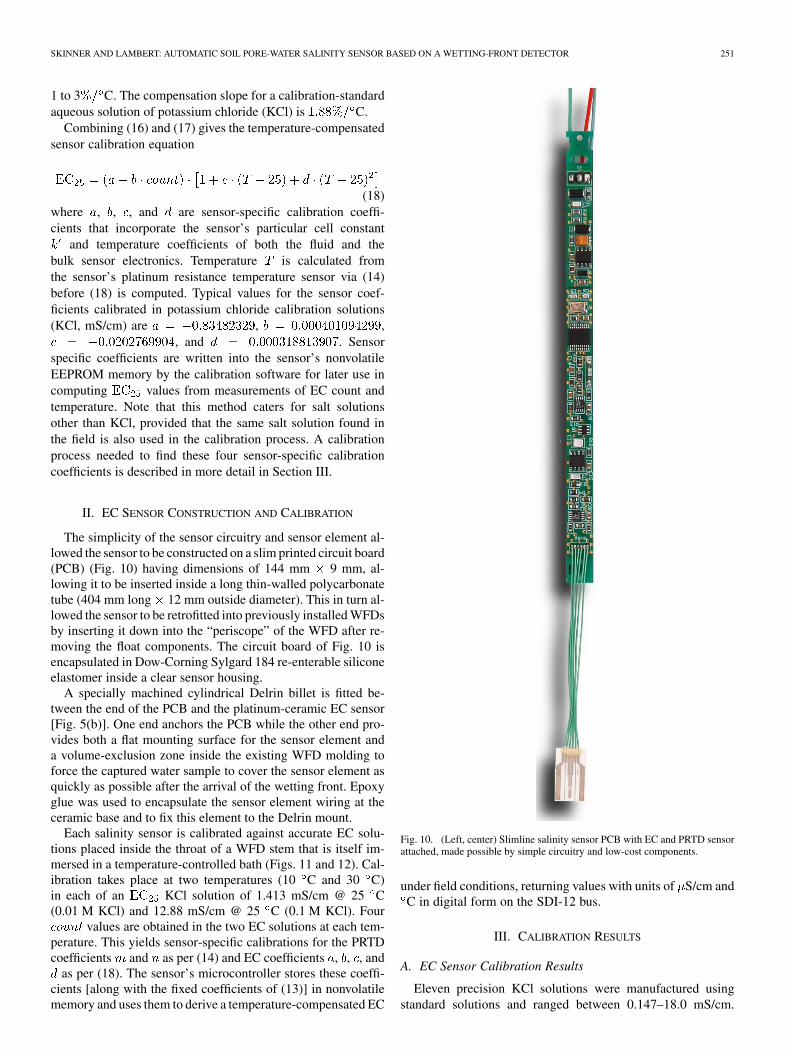
The simplicity of the sensor circuitry and sensor element al-lowed the sensor to be constructed on a slim printed circuit board(PCB) (Fig. 10) having dimensions of 144 mm 9 mm, al-lowing it to be inserted inside a long thin-walled polycarbonatetube (404 mm long 12 mm outside diameter). This in turn al-lowed the sensor to be retrofitted into previously installed WFDsby inserting it down into the “periscope” of the WFD after re-moving the float components. The circuit board of Fig. 10 isencapsulated in Dow-Corning Sylgard 184 re-enterable siliconeelastomer inside a clear sensor housing.

A specially machined cylindrical Delrin billet is fitted be-tween the end of the PCB and the platinum-ceramic EC sensor[Fig. 5(b)]. One end anchors the PCB while the other end pro-vides both a flat mounting surface for the sensor element anda volume-exclusion zone inside the existing WFD molding toforce the captured water sample to cover the sensor element asquickly as possible after the arrival of the wetting front. Epoxyglue was used to encapsulate the sensor element wiring at theceramic base and to fix this element to the Delrin mount.

Each salinity sensor is calibrated against accurate EC solu-tions placed inside the throat of a WFD stem that is itself im-mersed in a temperature-controlled bath (Figs. 11 and 12). Cal-ibration takes place at two temperatures (10 C and 30 C)in each of an KCl solution of 1.413 mS/cm @ 25 C(0.01 M KCl) and 12.88 mS/cm @ 25 C (0.1 M KCl). Four

values are obtained in the two EC solutions at each tem-perature. This yields sensor-specific calibrations for the PRTDcoefficients and as per (14) and EC coefficients , , , and

as per (18). The sensor’s microcontroller stores these coeffi-cients [along with the fixed coefficients of (13)] in nonvolatilememory and uses them to derive a temperature-compensated EC

Fig. 10. (Left, center) Slimline salinity sensor PCB with EC and PRTD sensorattached, made possible by simple circuitry and low-cost components.

under field conditions, returning values with units of S/cm andC in digital form on the SDI-12 bus.

III. CALIBRATION RESULTS

A. EC Sensor Calibration Results

Eleven precision KCl solutions were manufactured usingstandard solutions and ranged between 0.147–18.0 mS/cm.

252 IEEE SENSORS JOURNAL, VOL. 11, NO. 1, JANUARY 2011

Fig. 11. Isothermal insulated calibration tank with circulating pump (frontcenter) and a computer-controlled chiller (bottom-left) to force tank tem-peratures to high-low-middle temperatures of 10 C, 30 C, and 25 C,respectively, under computer control (center left). Sensor “salinity wells” canbe seen protruding from the top of the tank. The insulated tank lid is not shown.Automated computer-controlled calibration reduces the cost of manufacturing“smart sensors.”

Fig. 12. “Salinity wells” filled with EC solutions of either 1.413 or12.88 mS/cm (at 25 C) ready for submersion in the controlled temperaturebath. This allows simultaneous calibration of up to 12 EC sensors at one time.The salinity wells are shown lifted out of the water bath. The sensors are notinserted in this photograph for the sake of clarity.

Four sensors were tested in each solution inside salinity wellsin the calibration water bath shown in Fig. 12. Measurementuncertainties for all four sensors over this range fell within

1% of full scale.

B. PRTD Temperature Sensor Calibration Results

The PRTD temperature sensor is known for its repeatableand well-characterized temperature–resistance relationship and

would not normally require calibration. However, (8) and sub-sequent tests of the practical implementation of this low-costPRTD circuit, as described in Section II, showed that nonlineari-ties exist outside the sensor element in addition to that describedby the Callendar–Van Dusen equation. Careful measurementswere therefore undertaken for 12 randomly selected sensors inthe well-mixed calibration tank of Fig. 11 over 926 measure-ments per sensor between 8 C and 23 C against a precisionPRTD Fluke–Hart temperature standard, itself immersed in asalinity well in the center of the cluster.

The tank temperature was ramped upwards at a rate of ap-proximately 0.2 C per hour, this being the rate-of-heat gaindue to the mechanical action of the circulating pump used tominimize radial temperature gradients across the sensor cluster.Average deviation for all 12 sensors over 11 000 readings afterinternal linearization was 0.00 38 C, suggesting that the two-point linearization method is adequate for the intended applica-tion of soil salinity monitoring.

IV. FIELD RESULTS

A WFD was installed in February 2009 at 400-mm depthbelow Cabernet–Sauvignon vines in red sandy-loam soils at theYalumba “Oxford Landing” vineyard adjacent to the automaticvacuum sampler (Figs. 1–3). The salinity sensor of Fig. 10, suit-ably encapsulated, was installed in early September 2009 andconnected to a data logger and telemetry system that also mon-itored rainfall and soil moisture tension ( , kPa) at 300-mmdepth. Data was recorded every 15 min over the period betweenSeptember 24, 2009, and November 24, 2009, during the Aus-tralian spring (Fig. 13). This period of 62 days covered 17 irri-gation events and three significant rainfall events of 10.8 mm onOctober 2, 2009, 20.4 mm on November 3, 2009, and 48.4 mmon November 21, 2009. The first two rainfall events diluted thefollowing soil salinity reading slightly, with a significant reduc-tion of soil pore water salinity after the third event.

Analysis of each irrigation record (e.g., Fig. 14) showed thatwater entered the WFD funnel and rapidly filled the measure-ment space, resulting in a peak electrical conductivity. After thepassing of the wetting front, soil moisture tensions above thefunnel increase beyond 3 kPa and water wicks back out of themeasurement chamber, returning to the soil. The falling waterlevel in the chamber results in an apparent fall in electrical con-ductivity as the electrodes are progressively uncovered. The pas-sage of the wetting front takes between 3 and 4 h, with the mostaccurate salinity measurement being the peak EC value at theleading edge of the EC record.

As winter rainfall was consumed from the soil profile in earlyspring (September 2009) soil salinity fell somewhat from tem-perature-corrected EC values of 2000 to 1774 S/cm due to rain-fall. EC levels in the soil rose as the vine canopy developed andtranspiration increased, leaving salts to accumulate after the ap-plication of irrigation water having an average EC of approxi-mately 500 S/cm. The increasing frequency of irrigation eventscan be seen in the soil moisture trace as the weather warmed upthrough October and November. Soil solution EC rose to over5000 S/cm at 400-mm depth. The salinity spikes clearly co-incide with the irrigation events. The latter are marked by therapid fall in soil moisture tension values as the profile wets up.

SKINNER AND LAMBERT: AUTOMATIC SOIL PORE-WATER SALINITY SENSOR BASED ON A WETTING-FRONT DETECTOR 253

Fig. 13. Increasing soil pore water salinity as recorded by an instrumentedwetting-front detector at 400-mm depth in sandy-loam soil under vines at Ox-ford Landing vineyard near Waikerie in the South Australian Riverland. Thesoil moisture tension trace (dashed blue line (online version), shown as abso-lute values) at 300 –mm depth indicates an increase in the rate of soil moisturetake-up as the weather warms up and the vine canopy develops after grapevinesenescence over the winter period. Three significant rainfall events (green bars(online version), black arrows) result in dilution of the soil EC (red trace, onlineversion), as expected. The heavy black line joining wetting-front events showsthe EC trend. The triangular data points show the vacuum samples at 200 and400 mm averaged over the preceding two week period.

Fig. 14. Soil salinity readings during two consecutive irrigation cycles at Ox-ford Landing vineyard in South Australia around November 6, 2009. The wet-ting-front detector causes a small sample of a few cc of soil pore water to collectaround the four-electrode EC sensor; this sample “wicks” back into the soil overa 3–4-h period after the passing of the wetting front. The true sample EC is theinitial high reading—further readings fall away as the sample retreats from themeasurement cell, exposing the 1-cm-high electrode set and decreasing the “ap-parent” EC.

The vacuum soil salinity sampler at 200- and 400-mm depthare plotted in Fig. 13 as triangular points, showing similar trendsto the automated soil salinity sensor, but tending to lower valuesdue to the averaging effect of continuous vacuum sampling readat the end of each two week period. Soil salinity increases withdepth.

V. DISCUSSION AND CONCLUSION

A simple EC and temperature sensor has been developed andtested under laboratory and field conditions for the continuousmeasurement of soil-salinity samples collected in the throat of

a wetting front detector under soil moisture tension con-ditions between 0 and 3 kPa. As far as is practicable, vari-ations between individual sensors are ironed out via an auto-mated four-point calibration process that compensates for slightdifferences in cell-geometry and temperature coefficients of theelectronic measurement circuitry. Sensor measurement nonlin-earities are linearized via second-order polynomials. Simple cir-cuitry has been demonstrated that is capable of making high-res-olution measurements without the need for more expensive in-strumentation amplifiers and ADCs. Driving down sensor costis absolutely essential in soil salinity monitoring to compen-sate for the extensive variability of soil types across the land-scape. While debate continues in scientific circles as to whatactually constitutes a representative soil-salinity sample [7], thisapproach of monitoring salinity during periods when moistureis mobilized within the soil profile offers an affordable and log-gable solution suitable for long-term field studies.

ACKNOWLEDGMENT

The authors would like thank Dr. R. Stirzaker, CSIRO Landand Water, for providing encouragement and advice in the ap-plication of the sensor to the WFD. The authors would also liketo thank R. Iacobelli, G. Rouse, C. Bischoff, and J. Hoogland,Measurement Engineering Australia, for providing valuabletechnical assistance in manufacturing, programming, andtesting sensor prototypes.

REFERENCES

[1] L. J. Briggs and A. G. McCall, “An artificial root for inducing capillarymovement of soil moisture,” Science, vol. 20, pp. 566–569, 1904.

[2] S. Falivene, “Soil solute monitoring in Australia,” Cooperative Re-search Centre for Irrigation Futures, Irrigation Matters Series No.04/08, 2008.

[3] M. Inoue, N. Higashi, S. Yamazaki, K. Inosako, and Y. Mori, “Effect ofsalt concentration on measurement of soil water content using varioussoil moisture probes based on dielectric constant,” in Proc. ASA-CSSA-SSSA Int. Annu. Meetings, Seattle, WA, Oct. 31–Nov. 4 2004.

[4] M. Inoue, B. A. O. Ahmed, T. Saito, and M. Irshad, “Comparison oftwelve dielectric moisture probes for soil water measurement undersaline conditions,” Amer. J. Environ. Sci., vol. 4.4, pp. 367–372, Aug.2008.

[5] I. D. Jolly, T. I. Dowling, L. Zhang, D. R. Williamson, and G. R.Walker, “Water and salt balances of the catchments of the Murray-Dar-ling Basin,” CSIRO Tech. Rep. 37/97, Nov. 1997.

[6] A. Nadler, “Methodologies and the practical aspects of the bulk soilEC-soil solution EC relations,” Adv. Agronomy, vol. 88, pp. 273–312,2005.

[7] S. R. Raine, W. S. Meyer, D. W. Rassam, J. L. Hutson, and F. J. Cook,“Soil-water and solute movement under precision irrigation: Knowl-edge gaps for managing sustainable root zones,” Irrigation Sci., vol.26, pp. 91–100, 2007.

[8] F. Reverter and R. Pallàs-Areny, “Direct sensor-to-microcontroller in-terface circuits: Design and characterisation,” Marcombo S.A., 2005.

[9] E. Shuichi, I. Tsujii, M. Kawashima, and Y. Okumura, “A new methodof temperature-compensation of electrical conductivity using temper-ature-fold dependency of fresh water,” Limnol., vol. 9, pp. 159–161,2008, 10.1007/s10201-008-0248-2.

[10] A. J. Skinner and M. F. Lambert, “Using smart sensor strings for con-tinuous monitoring of temperature stratification in large water bodies,”IEEE Sensors J., vol. 6, no. 6, pp. 1473–1481, Dec. 2006.

[11] R. J. Stirzaker, “When to turn the water off: Scheduling micro-irrigationwith a wetting front detector,” Irrigation Sci., vol. 22, pp. 177–185,2003.

[12] R. J. Stirzaker, S. Sunassee, and J. Wilkie, “Monitoring water, nitrateand salt on-farm: A comparison of method,” in Proc. Irrigation Aus-tralia Conf., Adelaide, Australia, May 11–13, 2004, CSIRO Land andWater Tech. Rep. 34/04.

254 IEEE SENSORS JOURNAL, VOL. 11, NO. 1, JANUARY 2011

[13] R. J. Stirzaker and P. A. Hutchinson, “Irrigation controlled by a wettingfront detector: Field evaluation under sprinkler irrigation,” Aust. J. SoilRes., vol. 43, pp. 935–943, 2005.

[14] R. Stirzaker, “Factors affecting sensitivity of wetting front detectors,”Acta Hort., vol. 792, pp. 647–653, 2008.

Andrew J. Skinner received the B.Tech. and M.E.E.degrees from the South Australian Institute of Tech-nology, in 1975 and 1987, respectively, and the Ph.D.degree in engineering from the University of Ade-laide, Adelaide, South Australia, in 2009.

He has worked in Australia, Papua New Guinea,and Canada as a Nucleonic Instrumentation DesignEngineer in the mineral processing industry. Hereturned to Australia in 1982 to specialize in datalogging applications and environmental measure-ment systems, founding Measurement Engineering

Australia (MEA), Adelaide, in 1984. He is currently the Engineering Directorwith MEA.

Martin F. Lambert received the Ph.D. degree fromthe University of Newcastle, Newcastle, Australia.

He joined the University of Adelaide, Adelaide,South Australia, in 1995, where he is currently a Pro-fessor and Head of the Department of Civil, Environ-mental and Mining Engineering. His research areasinclude river hydraulics, pipeline condition assess-ment, and stochastic hydrology.