An Axiomatic Approach to Complete Patience and Time Invariance

journal of economic theory 83, 105�144 (1998)

An Axiomatic Approach to Complete Patienceand Time Invariance

Massimo Marinacci*

Department of Economics, University of Toronto, Toronto M5S 3G7, Canadamassimo�chass.utoronto.ca

Received October 24, 1997; revised May 4, 1998

The standard criterion used to compare streams of payoffs in the undiscountedcase is lim infT � � 1�T �T

t=1 u(xt). In this paper we approach the problemaxiomatically. This sheds light on the behavioral underpinnings of such a rule andleads to a novel choice criterion, the Polya Index. Journal of Economic LiteratureClassification Numbers: C72, C73, D90. � 1998 Academic Press

1. INTRODUCTION

In some intertemporal problems it is important to consider agents whodo not discount future utilities but instead attach the same importance toall periods, no matter how far apart they are. This is the case for a socialplanner who allocates resources among different generations, or for playerswho greatly value a long time horizon in a repeated strategic interaction.For instance, the celebrated folk theorems of Aumann and Shapley [1]and Rubinstein [20] consider complete patient players, as well as earlierworks on infinitely repeated stochastic games (see, e.g., Blackwell andFerguson [3]). Complete patient social planners have been considered ingrowth theory by the literature pioneered by Ramsey [19].

In the discounted case, the standard criterion used to compare infinitestreams of payoffs [x1 , ..., xn , ...] is (1&$) ��

t=1 $t&1 u(xt) for 0<$<1.Without discounting, it seems natural to focus on the limit of the timeaverages limT � � 1�T �T

t=1 u(xt). In particular, the following classicresult shows that this criterion can be thought of as the limiting case ofdiscounting.1

article no. ET972451

1050022-0531�98 �25.00

Copyright � 1998 by Academic PressAll rights of reproduction in any form reserved.

* I thank Larry Epstein, Itzhak Gilboa, Marco Scarsini, an anonymous referee, and par-ticipants at the Chantilly Workshop on Decision Theory, June, 1997, for some very usefuldiscussions. The financial support of the Social Sciences and Humanities Research Council ofCanada is gratefully acknowledged.

1 The `ìf '' part is due to Littlewood [13], while the more famous `ònly if '' part is due toFrobenius [8].

Theorem 1. Let [u(x1), ..., u(xn), ...] be a bounded stream of utilities. ThenlimT � � 1�T �T

t=1 u(xt) exists if and only if lim$ � 1 (1&$) ��t=1 $t&1 u(xt)

exists. In this case

limT � �

1T

:T

t=1

u(xt)= lim$ � 1

(1&$) :�

t=1

$t&1 u(xt).

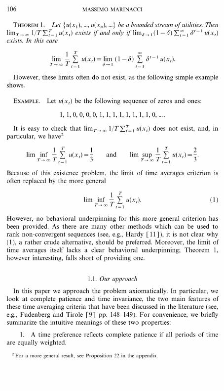
However, these limits often do not exist, as the following simple exampleshows.

Example. Let u(xt) be the following sequence of zeros and ones:

1, 1, 0, 0, 0, 0, 1, 1, 1, 1, 1, 1, 1, 1, 0, ... .

It is easy to check that limT � � 1�T �Tt=1 u(xt) does not exist, and, in

particular, we have2

lim infT � �

1T

:T

t=1

u(xt)=13

and lim supT � �

1T

:T

t=1

u(xt)=23

.

Because of this existence problem, the limit of time averages criterion isoften replaced by the more general

lim infT � �

1T

:T

t=1

u(xt). (1)

However, no behavioral underpinning for this more general criterion hasbeen provided. As there are many other methods which can be used torank non-convergent sequences (see, e.g., Hardy [11]), it is not clear why(1), a rather crude alternative, should be preferred. Moreover, the limit oftime averages itself lacks a clear behavioral underpinning; Theorem 1,however interesting, falls short of providing one.

1.1. Our approach

In this paper we approach the problem axiomatically. In particular, welook at complete patience and time invariance, the two main features ofthese time averaging criteria that have been discussed in the literature (see,e.g., Fudenberg and Tirole [9] pp. 148�149). For convenience, we brieflysummarize the intuitive meanings of these two properties:

1. A time preference reflects complete patience if all periods of timeare equally weighted.

106 MASSIMO MARINACCI

2 For a more general result, see Proposition 22 in the appendix.

2. A time preference is time invariant if the payoffs obtained in anyfinite number of periods do not matter.

In the paper we first study the second property. In particular, we provethat time invariance per se would deliver the following criterion:

limT � � _ inf

j�1 \1T

:T

t=1

u(xj+t)+& .

Notice that such a limit always exists.After having established this result, we focus on patience. Unlike time

invariance, complete patience is much trickier to axiomatize. In the finitecase there is a natural definition of complete patience: we have completepatience when the ordering of any two payoff streams does not change bytaking arbitrary permutations of their respective time indexes. However,we show that a literal translation of this definition to the infinite case ishighly unsatisfactory. In particular, it delivers the following criterion:

lim inft � �

u(xt),

where only instantaneous utilities are considered.To provide a more interesting definition of complete patience we use

natural densities. For a given subset of points of time A, its natural density$(A) is defined by

limt � �

|A & [1, ..., t]|t

whenever the limit exists, which is not always the case. Loosely speaking,a permutation x? of a payoff stream x=[xt]t�1 preserves the upper sets'densities if $([t: u(xt)�:])=$([t: u(x?

t )�:]) for all real numbers :.These permutations do not change the relative frequencies with which thedifferent payoffs come up in the stream (in section 6 a simple example isprovided).

We say that an agent is completely patient when the ordering of twopayoff streams does not change by taking permutations that preserve theupper sets' densities. This more compelling definition of patience delivers,up to a technical condition, the following criterion:

lim= � 0 _lim inf

T � �

1=T

:T

t=(1&=) T

u(xt)& . (2)

107COMPLETE PATIENCE

We call this criterion the Polya Index. It is well defined for every possiblebounded payoff stream. In particular,

lim= � 0 _lim inf

T � �

1=T

:T

t=(1&=) T

u(xt)&= limT � �

1T

:T

t=1

u(xt)

when the limit of time averages exists, so that the Polya Index extends thestandard limit criterion. This implies that our representation theoremprovides a foundation for the limit criterion as well.

The Polya Index has an interesting characterization. Let F be the set ofall bounded payoff streams, o

t a time preference on F that can berepresented by the Polya Index, and u(xt) its corresponding instantaneousutility. Let

Fa={x=[xt] t�1 # F: limT � �

1T

:T

t=1

u(xt) exists= ,

that is, Fa is the set of all payoff streams that have a well defined limit oftime averages. For any given stream x=[xt]t�1 , it holds that

P(x)=sup { limT � �

1T

:T

t=1

u(x$t): x$ # Fa and xotx$= , (3)

where P(x) denotes the Polya Index of the stream x. That is, the PolyaIndex of x is the supremum of the time average limits taken over allstreams x$ for which such a limit is well defined, and such that xo

tx$.Besides its intrinsic interest, this characterization, together with the

original form (2), seems to provide the Polya Index with an interestinganalytic tractability.3

1.2. Lim inf

Instead of deriving the standard lim inf criterion, our axiomaticapproach led us to the Polya Index. However, our analysis also sheds newlight on the lim inf criterion. To see why this is the case we have to makea short digression. This work started as a dividend of the analysis ofMarinacci [15]. In that paper it was shown that for any bounded sequence


3 As we will prove, it also holds that

P(x)=sup { limT � �

1T

:

T

t=1

u(x$t): x$ # Fa and u(x$t)�u(xt) for all t�1= .

This representation seems especially useful in terms of analytical tractability.

f : N � R there exists a non-additive normalized measure &: 2N � [0, 1]such that

lim infn

f (n)=| f (n) d&,

where an appropriate notion of integral, due to Choquet [5], is used (seethe appendix for details).

As Choquet integrals have been used to model vague subjective beliefs inSchmeidler [21], this observation suggested the possibility of using thatframework to study time preferences. It turned out, however, that the mostappropriate framework was the closely connected multiple priors model ofGilboa and Schmeidler [10].

We now illustrate this point. In our temporal context we have weightsinstead of priors, which represent how much the agents value the differentpoints of time. Combined with utilities, different weights deliver differentrankings of the payoff streams. In particular, a natural weight for completepatience would be the natural density defined above. However, this densityfails to exist for many sets, and so we cannot use it as a weight. Lackingthis `ìdeal'' weight, we assume that agents replace it with sets of weights,in particular with those weights that coincide with the natural densitywhenever it exists. This is why the multiple priors model is useful for ourpurposes.4

By using this model as our set-up we derive the Polya Index. Moreover,we show that there exists a strict subset Cl of the set of weights justdescribed such that

lim infT � �

1T

:T

t=1

u(xt)=min+ # Cl

| u(xt) d+. (4)

Even though we have not been able to determine which furtherrequirements on preferences are needed to move to the strict subset Cl , theequality (4) sheds light on the nature of the lim inf criterion, and on theway in which it combines weights and utilities. In particular, it provides anovel behavioral perspective on the lim inf criterion: an agent who usessuch a criterion can be viewed as using a set of weights, all coinciding withthe natural density when this `ìdeal'' weight exists. The set is then sum-marized through the minimum min+ # Cl

� u(xt) d+.


4 Of course, an alternative justification for this model in our temporal context is that theagents are not sure which weight to use and, instead of a single one, use a set of them. Thisjustification is, mutatis mutandis, more in line with the original argument of Gilboa andSchmeidler [10].

In sum, our axiomatic approach to time invariance and completepatience led to some new criteria to rank streams of payoffs, notably thePolya Index, and shed new light on the lim inf criterion, the most used inthe non discounted case. As a secondary contribution, we provide a con-nection between the two apparently unrelated issues of modelling vague-ness in subjective beliefs and complete patience in time preferences. Finally,in a companion paper, Marinacci [16], we show that our axiomaticapproach leads to a considerable generalization of the undiscounted FolkTheorems. Specifically, we show that they can be proved by imposing onlyconditions on preferences, without relying on any particular evaluationfunctionals. In so doing, we generalize and unify several important resultsobtained in the case of complete patience, included the classic results ofAumann and Shapley [1] and Rubinstein [20]. Moreover, our results arebased only on properties of preferences and this makes transparent theirbehavioral foundation.

The rest of the paper is organized as follows. Section 2 describes the set-up, and reports the representation theorem of Gilboa and Schmeidler [10].Section 3 examines time invariance, and proves a representation resultfor this property. Section 4 considers the ``naive'' definition of completepatience, and shows what kind of representation result it entails. Section 5shows how unsatisfactory the naive definition is and argues that naturaldensities have to be considered. It also shows that a form of patience isalready incorporated in the time invariance axiom. Section 6 formallydefines patience by means of densities, and proves the relative representa-tion theorem, where the Polya Index first occurs. Section 7 provides twointeresting characterizations of the Polya Index. Finally, section 8 considersthe lim inf criterion, and shows that our analysis sheds new light on thiscriterion as well. All the proofs, and the most technical analysis, arerelegated to the appendix. A glossary of the more relevant notation isprovided at the beginning of the appendix.

2. SET-UP

We use the generalization of the Anscombe�Aumann model introducedin Gilboa and Schmeidler [10] and Schmeidler [21].

Let X be a nonempty set of consequences and P the set of all probabilitydistributions with finite support on X, i.e.,

P={ p: X � [0, 1] : p(c){0 for finitely many c's in X and :c # X

p(c)=1= .


Let T=[1, ..., t, ...] be the set of points of time, and 2T its power set.An act f is a function from T into P. For p # P, p* denotes the constantact p*(t)= p for all t # T.

The set of all acts is endowed with a preference ordering ot . In par-

ticular, F denotes the set of all bounded acts, i.e., f # F if there arep1 , p2 # P such that p*1 O

t f Ot p*2 for all t # T.

We now present several axioms on ot .

A.1. Weak Order. ot is complete and transitive.

A.2. Monotonicity. For all acts f, g # F we have f ot g whenever

f (t)ot g(t) for all t # T.

A.3. Continuity. For all f, g, h # F, if f o g and goh, then there are:, ; # (0, 1) such that :f +(1&:) ho go;f +(1&;) h.

A.4. Nondegeneracy. There exist f, g # F such that f o g.

All the above axioms are standard, and have a simple interpretation. Thenext axiom is a weak version of the Independence Axiom, which onlyrequires independence with respect to constant acts.

A.5. Certainty Independence. For all acts f and g, for all constant actsc, and all 0<:<1, f o

t g if and only if :f +(1&:) cot:g+(1&:) c.

Next we introduce a smoothing axiom: the agent always weakly prefersto smooth his payoff stream by mixing two indifferent acts rather than haveonly one of them all the time.

A.6. Intertemporal Smoothing. For all f and g in F, f t g implies:f +(1&:) go

t f for all 0<:<1.

Finally, a key ingredient in a temporal decision is how the agents weightthe different points of time. In this set-up, where infinite points of time areconsidered, formally a weight is a set function +: 2T � [0, 1] that satisfiesthe following conditions:

(i) +(<)=0;

(ii) +(A _ B)=+(A)++(B) whenever A & B=<;

(iii) +(T)=1.

We can now report the Gilboa and Schmeidler Theorem for our set-up(Chateauneuf [4] proved independently a similar result).


Theorem 2. The following two statements are equivalent:

(i) The preference relation ot on F satisfies the axioms A.1�A.6.

(ii) There exists an affine real valued function u on P and a uniquenon-empty weak*-compact and convex set C of weights on 2T such that, forall f and g in F,

f ot g if and only if min

+ # C|

T

u( f (t)) d+�min+ # C

|T

u(g(t)) d+.

Finally, the function u is unique up to a positive linear transformation.

Interpreted in our temporal context, this representation means that theagent does not evaluate the payoff streams through a single weight,but instead uses a set of weights, summarized by the minimummin+ # C �T u( f (t)) d+.

By Theorem 2, every preference relation ot that satisfies axioms A.1-A.6

is associated with a pair (u, C), the utility function on P and the set ofmultiple weights. Using these pairs it is possible to introduce a natural par-tial order R on the set of preference relations satisfying axioms A.1�A.6:We write o

tRot $ if the two following conditions are satisfied:

(i) the utility functions u and u$ on P are equal, up to positive lineartransformations;

(ii) the set C$ is contained in C, i.e., C$�C.

The partial order R is reflexive, transitive, and antisymmetric. It is easyto see that for two preferences o

t and ot $ satisfying axioms A.1�A.6, the

following two statements are equivalent:

(i) otRo

t $

(ii) for all f # F and all constant acts p* it holds that

p*ot $f implies p*o

t fp*o $f implies p*o f.

Definition 3. Let ot be a preference relation that satisfies a given set

of axioms, which includes A.1�A.6. We call ot canonical if o

tRot $ for all

other preferences ot $ that satisfy the same set of axioms.

In other words, a preference relation ot that satisfies a given set of

axioms is canonical if it holds that C$�C for all preferences ot $ which

satisfy the same set of axioms and have the same utility function on P.


It is important to keep in mind that ot is canonical with respect to a

given set of axioms. Indeed, different sets of axioms may be associated withdifferent canonical preference relations.

2.1. Comonotonic Independence

In the sequel we will need another axiom, due to Schmeidler [21]. Twoacts f and g in F are comonotonic if for no t, t$ # T it holds f (t)o f (t$)and g(t)O g(t$). In other words, f (t)o f (t$) implies g(t)o

t g(t$), i.e., twocomonotonic acts have the same kind of monotonicity. Consequently, theirintertemporal payoff profile has a similar shape and the mixture of twocomonotonic acts does not alter the shape. It therefore seems natural torequire that this mixture does not change the original preference orderingbetween the two acts. This motivates the next axiom, a stronger versionof A.5.

A.7. Comonotonic Independence. For all pairwise comonotonic actsf, g, h # F and all : # (0, 1), f o

t g implies :f +(1&:) hot:g+(1&:) h.

This axiom plays an important role in the representation theorem fornon-additive measures proved in Schmeidler [21], which is reported in theappendix.

3. TIME INVARIANCE

We first study time invariance. Given an act f # F, define

f k (t)= f (t+k) for all t�1.

A.8*. Time Invariance. For every f # F and every k>0 it holds thatf t f k.

According to this axiom, the agent puts zero weight on the consequencesobtained on all past and present periods, and full weight to the futureperiods. In other words, it does not matter what happens in any finite setof points of time.

A crucial implication of Theorem 1 is that Time Invariance must besatisfied by any preference relation that aims to model the undiscountedcase as a limit case of discounting as $ goes to 1, when such a limit exists.This is a very important feature of Time Invariance.

In the sequel we will sometimes need a very weak independence axiomrelated to time invariance. A bit of notation: For a set of points of time


A�T, and for a pair p1 , p2 # P, with p2o p1 , let fA be the act definedby:

fA (t)={ p2 if t # Ap1 if t � A.

In other words, fA is any binary act which gives a higher payoff on Athan on Ac. In the notation fA we omit explicit reference to p1 and p2 sincewhat matters is only their relative order, not their specific values.

A.8. Time Invariance Independence. For all A�T there exist a fA # F

such that

12 fA+ 1

2 fAc t12 f k

A+ 12 fAc

for all k�1.

This is a very weak notion of independence, and it only involves timeinvariance. Interestingly, it turns out that A.8 implies A.8* (this is why wehave used the star in A.8*).

Proposition 4. Suppose the preference relation ot on F satisfies

axioms A.1�A.6 and A.8. Then, it satisfies A.8*. The converse is false (thatis, there exist preference relations o

t on F that satisfy axioms A.1�A.6 andA.8*, but not A.8).

An example of a utility functional that satisfies A.8* but not A.8 is

lim inft � �

u( f (t)),

i.e., the lim inf of instantaneous utilities.

3.1. A Representation

As will be proved in the appendix, A.8 implies in terms of multipleweights that all the weights have to be invariant.5 As there is no a priorireason to exclude any of these invariant weights, we focus on the maximalset of invariant weights. In other words, we focus on the canonicalpreference relation that satisfies the set of axioms A.1�A.6 and A.8.

For the canonical preference relation we obtain the following representa-tion result, which provides a complete characterization of time invariancefor this natural case.


5 Let x=[xn]n�1 be a bounded sequence, and { the shift transformation defined by

({(x))n=xn+1

for all n�1. A weight +: 2T � [0, 1] is invariant if +(A)=+({(A)) for all A�T.


(i) The preference relation ot on F is canonical and satisfies axioms

A.1�A.6 and A.8.

(ii) There exists an affine real valued function u on P such that, for allf and g in F, we have, f o

t g if and only if

limT � � _ inf

j�1 \1T

:T

t=1

u( f ( j+t))+&� limT � � _ inf

j�1 \1T

:T

t=1

u(g( j+t))+& .


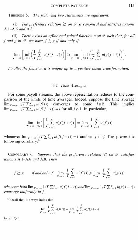
3.2. Time Averages

For some payoff streams, the above representation reduces to the com-parison of the limits of time averages. Indeed, suppose the time averagelimT � � 1�T �T

t=1 u( f (t)) converges to some l # R. This implieslimT � � 1�T �T

t=1 u( f ( j+t))=l for all j�1. In particular,

limT � �

infj�1 _

1T

:T

t=1

u( f ( j+t))&= limT � �

1T

:T

t=1

u( f (t))

whenever limT � � 1�T �Tt=1 u( f ( j+t))=l uniformly in j. This proves the

following corollary.6

Corollary 6. Suppose that the preference relation ot on F satisfies

axioms A.1�A.6 and A.8. Then

f ot g if and only if lim

T � �

1T

:T

t=1

u( f (t))� limT � �

1T

:T

t=1

u(g(t))

whenever both limT � � 1�T �Tt=1 u( f ( j+t)) and limT � � 1�T �T

t=1 u(g( j+t))converge uniformly in j.


6 Recall that it always holds that

limT � �

1T

:

T

t=1

u( f (t))= limT � �

1T

:

T

t=1

u( f ( j+t))

for all j�1.

4. PATIENCE

We now move to the analysis of patience. As was mentioned in the intro-duction, there is a natural definition of complete patience in the finite case:we have complete patience when the ordering of any two acts does notchange by taking arbitrary permutations of their respective time indexes.

It is therefore natural to first look at the direct counterpart in the infinitecase of this notion, which is so compelling in the finite case. To do so, let6 be the set of all one-to-one and onto maps ?: T � T. Given an actf # F and a map ? # 6, define

f ? (t)= f (?(t)) for all t�1.

The act f ? is obtained from f through a rearrangement of its elements f (t).

A.9. Naive Patience. For every f # F and every ? # 6, it holds thatf t f ?.

This axioms states that the agent evaluates the consequences per se,regardless of the points of time where he gets them. This axiom charac-terizes an agent with `ìnfinite'' patience for whom all the points of time, nomatter how remote, have the same weight. We use the adjective naivebecause this is the literal translation in the infinite case of the naturalnotion of patience for finite sets. As will be seen, axiom A.9 is not at allsatisfactory. However, before moving on, we show what kind of representa-tion it entails.


(i) The preference relation ot on F satisfies the axioms A.1�A.4, A.6,

A.8*, and A.9.

(ii) There exists an affine utility u: P � R such that, for all f and g in F,

f ot g if and only if lim inf

t � �u( f (t))�lim inf

t � �u(g(t)). (5)

The function u is unique up to a positive linear transformation.

Notice that we use the lim inf of the instantaneous utilities and not oftheir time averages. It is worth noting that we obtain lim sup instead oflim inf in Eq. (5) if we replace A.6 with the dual axiom in which f t gimplies :f +(1&:) gO

t f for all 0<:<1. Similar dual versions hold for allthe representation results in the paper in which lim inf and min occur.


5. PATIENCE REVISITED

Axiom A.9, which is the literal translation of complete patience from thefinite to the infinite horizon, is much stronger than it might seem at a firstglance. For example, consider the two acts f and g defined as follows

f (t)={ p2 if t # [2k]k�1

p1 if t � [2k]k�1

and g(t)={ p2 if t # [4k]k�1

p1 if t � [4k]k�1

(6)

where p2 o p1 . It is easy to check that, according to A.9, it holds thatf t g. However, the relative frequency limt � � ( |[2k]k�1 & [1, ..., t]| )�t=1�2 with which the agent gets the higher consequence p2 under act f,is twice than that under g, i.e., limt � � ( |[4k]k�1 & [1, ..., t]| )�t=1�4.Nevertheless, by A.9, f t g because this axiom does not take into accountthe relative frequencies with which payoffs come up.

As this example suggests, we must modify A.9 in order to take care ofthe relative frequencies. In order to do this, we have to introduce densities.

Definition 8. Let A�T. The lower natural density of A is

$*

(A)=lim inft � �

|A & [1, ..., t]|t

,

while the upper natural density is

$*(A)=lim supt � �

|A & [1, ..., t]|t

.

Finally, a set A�T has natural density $(A) if $*

(A)=$*(A)=$(A).

The collection Ad=[A�T: $(A) exists] has the following properties:

1. A # Ad implies Ac # Ad ;

2. if A, B # Ad and A & B=<, then A _ B # Ad .

However, Ad is not an algebra.

5.1. Patience and Time Invariance

A form of patience based on frequencies is already implicit in the TimeInvariance axiom A.8. To see it, we need the following definition.


Definition 9. The lower Banach density of a set A�T is

;*

(A)= limT � � _ inf

j�1

|A & [ j, ..., j+T&1] |T & ,

while the upper Banach density is

;*(A)= limT � � _sup

j�1

|A & [ j, ..., j+T&1]|T & .

Finally, a set A�T has Banach density ;(A) if ;*

(A)=;*(A)=;(A).

It holds that

;*

(A)�$*

(A)�$*(A)�;*(A)

for all A�T. In particular, ;(A)=$(A) whenever ;(A) exists.Ab is the collection of all sets that have a Banach density, i.e.

Ab=[A�T: ;(A) exists], and Fb is the set of all acts f # F such that[t: f (t)o

t p] # Ab for all p # P.Given an act f # Fb , we are interested in permutations ? # 6 which are

invariant under Banach densities, i.e., ;([t: f (t)ot p])=;([t: f ? (t)o

t p])for all p # P. We denote them by 6 f

b .We can now state the notion of patience that comes with Time

Invariance.

Theorem 10. Suppose the preference relation ot on F satisfies axioms

A.1�A.6, and A.8. Then, for every f # Fb and every ? # 6 fb , it holds that

f t f ?.

6. PATIENCE AND DENSITIES

We have seen how Time Invariance implies a form of patience based onBanach densities. A natural step is to replace Banach densities with naturaldensities in the notion of patience implied by Time Invariance.

To do this, we need a bit of notation. Denote by Fd be the set of all actsf # F such that [t: f (t)o

t p] # Ad for all p # P. For a given f # Fd , denoteby 6 f

d the set of all permutations ? # 6 invariant under natural densities,that is, $([t: f (t)o

t p])=$([t: f ? (t)ot p]) for all p # P.

We are now in a position to state the new patience axiom.

A.10. Cardinal Patience. For every f # Fd and every ? # 6 fd , it holds

that f t f ?.


Of course, A.9 implies A.10, while the converse is not true. Moreover, ifwe replace Fd and 6 f

d with, respectively, their subsets Fb and 6 fb , by

Theorem 10 the axiom becomes a consequence of Time Invariance.The following simple example further illustrates the nature of this axiom.

Example. Let f # F be an act such that

f (t)={ p1 if t is even,p2 if t is odd,

with p1 o p2 . Clearly, f # Fd . Let ? be the permutation defined as follows:?(2t&1)=2t and ?(2t)=2t&1 for t�1. Then

f ? (t)={ p1 if t is odd,p2 if t is even.

This permutation preserves the upper sets' densities, i.e., ? # 6 fd . In fact

$([t: f (t)ot p])=$([t: f ? (t)o

tp])=1 if pOt p2

$([t: f (t)ot p])=$([t: f? (t)o

t p])= 12 if p2 O pO

t p1

$([t: f (t)ot p])=$([t: f? (t)o

t p])=0 if po p1

6.1. A Technical Condition

For the representation result we need a technical condition, calledregularity. It is introduced in this subsection, which can be skipped at afirst reading.

For any p̂ # P, let [ p̂]=[ p: pt p̂], i.e., [ p̂] is the indifference class con-taining p̂. Similarly, for A�P set [A]=[[ p]: p # A].

Definition 11. For a given f # F, let Af=[ p: [t: f (t)ot p] � A$]. We

denote by F$ the set of all acts f # F such that the set [Af] is at mostcountable.

In other words, if u: P � R is an affine utility associated with ot , F$ is

the set of all acts f such that [t: u( f (t))�:] � Ad for an at most countableset of : # R. Loosely speaking, F$ is the set of acts ``measurable'' w.r.t. A$ .Notice that Fd �F$ .

As will be seen in the appendix, if f # F$ , and p0 # P is such thatu( p0)=0, then f t p0 whenever

:�

t=1

u( f (t))t


converges (i.e., limT � � �Tt=1 u( f (t))�t) exists7 and is finite). For our next

representation theorem, a similar property must hold for all acts in F. Tothis end we introduce the following technical condition, called regularity.

Definition 12. Let ot be a preference ordering that satisfies A.1�A.6,

and u: P � R an affine utility provided by Theorem 2. Let p0 # P be suchthat u( p0)=0. We say that o

t is regular if, for all acts f # F�F$ such that

:�

t=1

u( f (t))t

converges and such that inft�1 u( f (t))<0<supt�1 u( f (t)), it holds thatf t p0 .8

We conclude by presenting an interesting class of acts in F$ .

Proposition 13. Let ot be a preference ordering that satisfies A.1�A.6,

and u: P � R an affine utility provided by Theorem 2. Let f # F. If thereexists an l # R such that

limT � �

1T

:T

t=1

|u( f (t))&l |=0, (7)

then f # F$ .

Remarks. (i) It is easy to check that (7) holds whenever limt � � u( f (t))exists. Hence, by Proposition 13, in this special case f # F$ . (ii) Ifu( f (t))�0 for all t�1 and ��

t=1 u( f (t))�t converges, then, by Kronecker'sLemma

limT � �

1T

:T

t=1

u( f (t))= limT � �

1T

:T

t=1

|u( f (t))|=0.

Hence, f # F$ by Proposition 13. This is why in Definition 12 we requirethat inft�1 u( f (t))<0<supt�1 u( f (t)). Otherwise, as just proved, f wouldautomatically be in F$ .


7 By Kronecker's Lemma, the convergence of ��t=1 u( f (t))�t implies limT � � 1�T

�Tt=1 u( f (t))=0. However, the converse is false. For example, let u( f (t))=1�lgt. Then

��t=1 1�tlgt=�, but limT � � 1�T �T

t=1 1�lgt=0.8 It is important to note that, as shown in the last footnote, the convergence of

��t=1 u( f (t))�t is a much stronger requirement on f than limT � � 1�T �T

t=1 u( f (t))=0.Therefore, regularity is a much weaker condition than assuming f t p0 whenlimT � � 1�T �T

t=1 u( f (t))=0.

6.2. Representation Theorem

We can now state the representation result.


(i) The preference relation ot on F is canonical, satisfies axioms

A.1�A.6, A.8�A.10, and is regular.

(ii) There exists an affine utility u: P � R such that, for all f and g inF, we have f o

t g if and only if

lim= � 0 _lim inf

T � �

1=T

:T

t=(1&=) T

u( f (t))&� lim= � 0 _lim inf

T � �

1=T

:T

t=(1&=) T

u(g(t))& .


Given its importance in this work, we now give a name to the functionalthat comes up in Theorem 14.

Definition 15. Let f # F and u: P � R an affine utility function. Thefunctional P : F � R defined by

P( f )= lim= � 0 _lim inf

T � �

1=T

:T

t=(1&=) T

u( f (t))&is called the Polya Index.

Remark. We call P the Polya Index because for the special case of actsf such that u( f (t)) # [0, 1] for all t�1, P( f ) is equal to the Polya minimaldensity of the set [t: u( f (t))=1]. These densities have been introduced byPolya [18, pp. 556�568].

Notice that

lim= � 0 _lim inf

T � �

1=T

:T

t=(1&=) T

u( f (t))&= limT � �

1T

:T

t=1

u( f (t)) (8)

whenever the limit on the r.h.s. exists. Therefore, the Polya Index is anextension of the limit of time average criterion to streams that do not havewell defined time average limits.

Using the equality (8), we get the following interesting consequence ofTheorem 14. It provides a behavioral underpinning for the use of timeaverages, provided they exist.


Corollary 16. Suppose the preference relation ot on F satisfies

axioms A.1�A.6, A.8, and A.10, and regularity. Then there exists an affineutility u: P � R such that, for all f and g in F,

f ot g if and only if lim

T � �

1T

:T

t=1

u( f (t))� limT � �

1T

:T

t=1

u(g(t)),

provided the two limits exist. The function u is unique up to a positive lineartransformation.

7. THE POLYA INDEX

We now provide two further characterizations of the Polya Index.

7.1. Polya Index as an Inner Approximation

We first characterize the Polya Index as an inner approximation. For agiven f # F, let Fa=[ f # F: limT � � 1�T �T

t=1 u( f (t)) exists].

Theorem 17. Let ot be the preference ordering of Theorem 14, and

u: P � R its corresponding affine utility. If u(P)=R (i.e., the range of u isR), for all f # F it holds that

P( f )=sup { limT � �

1T

:T

t=1

u(g(t)): g # Fa and f ot g= .

This characterization shows that the Polya Index can be viewed as aninner approximation taken over the less preferred acts that have welldefined time average limits. In other words, comparing two acts throughthe Polya Index is equivalent to comparing them by taking the supremumover the set of all less preferred acts which have well defined time averagelimits.

The proof of Theorem 17 rests on the following Lemma, which is inter-esting in itself because it provides the Polya Index with further analyticaltractability.

Lemma 18. Let u: P � R be the affine utility provided by Theorem 14. Ifu(P)=R, then, for all f # F, it holds that

P( f )=sup { limT � �

1T

:T

t=1

u(g(t)): g # Fa and u( f (t))�u(g(t)) for all t�1= .


7.2. Polya Index and Weights

Next we characterize the Polya Index in terms of sets of weights. Let{: T � T be the shift transformation defined by

{(t)=t+1.

We denote by Nd the set of all normalized finitely additive measures + on2T such that

1. +(A)=$(A) for all A # Ad .

2. +(A)=+({(A)) for all A�T, i.e., + is invariant w.r.t. {.

Besides being invariant, the weights in Nd coincide with the natural den-sity when it exists. They are the natural weights for complete patience (seethe discussion below), and the next result shows that the Polya Index canbe justified through them.

Theorem 19. Let u: P � R be the affine utility provided by Theorem 14.Then there exists a unique weak*-compact and convex set Cp�Nd such that

P( f )=min+ # Cp

| u( f (t)) d+

for all f # F.

Notice that up to a mild technical condition (i.e., regularity), the set Cp

coincides with Nd . The set Nd consists of all invariant weights that coincidewith the natural density $ whenever it exists. The density $ would be thenatural weight for complete patience, but it fails to exist for many sets andcannot be used as a weight. Lacking this `ìdeal'' weight, we can think ofan agent using the Polya Index as replacing it with the set of all invariantweights that coincide with $ whenever it exists, i.e., with the set Nd .9

This interpretation of the Polya Index was already outlined in the intro-duction and it is important because it provides the Polya Index with abehavioral foundation. Interestingly, this interpretation is completely dif-ferent from that used in the multiple priors model of Gilboa andSchmeidler, whose aim is to model vagueness in subjective beliefs.


9 It is important to note that the fact that the agent uses all the weights compatible with$ is the reason why in Theorem 14 we have a canonical ordering.

8. LIM INF OF TIME AVERAGES

In the last Theorem we have seen how the Polya Index can be represen-ted in terms of weights in Nd . We now show that the same is true for thelim inf of time averages.

Theorem 20. Let ot be a preference relation on F that satisfies axioms

A.1�A.6, A.8, and A.10, and regularity. Then there exists an affine utilityu: P � R and a unique non-empty weak*-compact and convex set Cl �Nd ofweights on 2T such that, for all f and g in F,

f ot g if and only if min

+ # Cl|

T

u( f (t)) d+�min+ # Cl

|T

u(g(t)) d+

and

min+ # Cl

|T

u( f (t)) d+=lim infT � �

1T

:T

t=1

u( f (t)).


This result shows that we can justify lim infT � � 1�T �Tt=1 u( f (t))

through a set of weights Cl contained in Nd . In particular, Cl % Cp , as thefollowing result shows.

Proposition 21. Cl % Cp .

The set Cl is therefore strictly smaller than Cp . Some weights in Cp haveto be eliminated in order to represent lim infT � � 1�T �T

t=1 u( f (t)).However, it is not clear what conditions on o

t , on top of A.1�A.6, A.8,A.10 and regularity, would lead to this elimination. In other words, it is notclear which further axiom to impose on o

t in order to move from Cp to thesmaller set Cl .

Therefore, the behavioral underpinning of the liminf criterion is lesstransparent than that of the Polya Index. Nevertheless, Theorem 20 isinteresting because it sheds light on the liminf criterion by providing arepresentation where weights and utilities are clearly separated.

9. PROOFS AND RELATED ANALYSIS

9.1. Glossary of notation

T set of points of time (sect. 2)X set of consequences (sect. 2)


P set of all probability distributions with finite support (sect. 2)F set of all bounded acts (sect. 2)C set of weights (sect. 2)

Fb set of all bounded acts that preserve the upper sets'Banach densities (sect. 5.1)

Fd set of all bounded acts that preserve the upper sets'natural densities (sect. 6)

Fa set of all bounded acts that have a well defined limitof time averages (sect. 7.1)

f k shift (sect. 3); Banach density (sect. 5.1)$ natural density (sect. 5)

6 set of all one-to-one and onto permutations on T (sect. 4)6 f

b set of all permutations invariant under Banach densities (sect. 5.1)6 f

d set of all permutations invariant under natural densities (sect. 6)Ab collection of all sets that have a Banach density (sect. 5.1)Ad collection of all sets that have a natural density (sect. 6)Nd invariant weights that coincide with the natural density

when it exists (sect. 7.2)

9.2. Example

In the introduction we presented an example of a sequence whose limitaverage does not exist. We now give a more general result that includes theexample as a special case. It shows how far apart can be the upper andlower bounds of the partial sums 1�T �T

t=1 xt .

Proposition 22. For any positive integer N there exists a sequence xsuch that xt # [0, 1] for all t�1, and

lim infT � �

1T

:T

t=1

xt=1

1+Nand lim sup

T � �

1T

:T

t=1

xt=N

1+N.

Notice that the difference

lim supT � �

1T

:T

t=1

xt&lim infT � �

1T

:T

t=1

xt=N&1N+1

tends to 1 as N gets larger and larger. As x takes on only the values 0 and1, this means that there are sequences for which the lim inf and lim sup arevery far away.

Proof. Given N, let x be the sequence whose first N elements are 1, thesecond N2 elements are 0, the third N 3 elements are 1, and so forth. It iseasy to check that


lim supT � �

1T

:T

t=1

xt= limT � �

�Tt=0 N2t+1

�Tt=0 N 2t+1+:T

t=0 N2t&1=

NN+1

lim infT � �

1T

:T

t=1

xt= limT � �

�Tt=0 N2t+1

�Tt=0 N 2t+1+:T

t=0 N2t&1+N2T+2

=1

N+1

as wanted. K

9.3. Proposition 4 and Theorem 5

Let l� be the set of real sequences x=[xn]n�1 bounded w.r.t. the sup-norm &x&=supn |xn |, and let {: l� � l� be the shift transformation definedby

({(x))n=xn+1 .

A linear functional L: l� � R is a Banach limit if it satisfies the followingconditions.

1. L(x)�0 if x�0.

2. L({(x))=L(x) for all x # l�.

3. L(1)=1, where 1 denotes the sequence [1, ..., 1, ...].

We denote by L the set of all Banach limits on l�.A finitely additive measure +: 2T � [0, 1] is invariant if +(A)=+({(A))

for all A�T. We denote by N the set of all finitely additive invariantmeasures. Let F: T � R be a sequence in l�. Set M=[� F d+: + # N]. Wehave

Lemma 23. L=M.

Proof. We first notice that, by Sucheston [22], limn supj�1

[1�n �nj=1 F(i+ j)] exists for all F # l�. We now prove that M�L. For all

A�T, let {&1 (A)=[t # T: {(t) # A]. We have {&1 ({(A))=A for allA�T, {({&1 (A))=A if [1] / A, and {({&1 (A)) _ [1]=A if [1]�A(notice that {({&1 (A)) & [1]=< in this last case). For every + # N itholds that +(A)=+({({&1 (A)))=+({&1 (A)) because +([1])=0. We have1A ({(t))=1{&1(A) (t), so that

| 1A ({(t)) d+=| 1A (t) d+ for all A�T. (9)


Let F # l� be a simple function. Using (9), it is easy to check that forevery invariant measure in N it holds that

| F d+=| _1n

:n

i=1

F(i+ j)& d+ for all j�1.

Therefore, � F d+�sup j�1 1�n �nj=1 F(i+ j), so that

| F d+�limn

supj�1 _

1n

:n

i=1

F(i+ j)& . (10)

Let F # l�. There exists a sequence of simple functions Fk that convergesuniformly to F. We can write

limn

supj�1 _

1n

:n

i=1

F(i+ j)&=limn

supj�1 _

1n

:n

i=1

limk

Fk (i+ j)&=lim

nsupj�1

limk _1

n:n

i=1

Fk (i+ j)& .

For every =>0 there exists K=>0 such that |F(i)&Fk (i)|<= for all k�K=

and all i�1. Hence

} 1n :n

i=1

Fk ( j+i)&1n

:n

i=1

F( j+i) }�

1n

:n

i=1

|Fk ( j+i)&F( j+i)|==

for all k�K= and all j�1. This implies that

limn

supj�1

limk _1

n:n

i=1

Fk (i+ j)&=limn

limk

supj�1 _

1n

:n

i=1

Fk (i+ j)& .

On the other hand, assume supj�1 1�n �ni=1 F(i+ j)�supj�1 1�n �n

i=1 Fk(i+j).Then

supj�1

1n

:n

i=1

F(i+ j)&supj�1

1n

:n

i=1

Fk (i+ j)

=supj�1

1n

:n

i=1

[F(i+ j)&Fk (i+ j)+Fk (i+ j)]&supj�1

1n

:n

i=1

Fk (i+ j)

�supj�1

1n

:n

i=1

[F(i+ j)&Fk (i+ j)]<=


for all k�K= and all n�1. The same holds if sup j�1 1�n �ni=1 F(i+ j)<

supj�1 1�n �ni=1 Fk (i+ j), so that

} supj�1

1n

:n

i=1

F(i+ j)&supj�1

1n

:n

i=1

Fk (i+ j) }<=

for all k�K= and all n�1. In turn, this implies

limn

limk

supj�1 _

1n

:n

i=1

Fk (i+ j)&=limk

limn

supj�1 _

1n

:n

i=1

Fk (i+ j)&and we conclude that

limn

supj�1 _

1n

:n

i=1

F(i+ j)&=limk

limn

supj�1 _

1n

:n

i=1

Fk (i+ j)& . (11)

Putting together (10) and (11), we get

| F d+=limk | Fk d+�lim

klim

nsupj�1 _

1n

:n

i=1

Fk (i+ j)&=lim

nsupj�1 _

1n

:n

i=1

F(i+ j)& .

Sucheston [22] proves that

limn

supj�1 _

1n

:n

i=1

F(i+ j)&= supm1, ..., ms _lim inf

j � �

1s

:s

k=1

F(mk+ j)& .

As � F d+ is a linear functional on l�, by Banach [2]

| F d+� supm1, ..., ms _lim inf

j � �

1s

:s

k=1

F(mk+ j)&implies that � F d+ is a Banach limit. This proves that M�L.

As to the converse, for any L # L there exists a finitely additive measureon 2T such that L(F )=� F d+ for all F # l� (cf. Dunford and Schwartz [6,p. 258]). But L(1A)=L(1{(A) ({(t)))=L(1{(A)), so that +(A)=+({(A)), i.e.+ # N. This implies L�M. K

Lemma 24. Suppose the preference relation ot satisfies axioms A.1�A.6,

and let C be the convex and compact set provided by Theorem 2. ThenC�N if and only if o

t satisfies A.8.

Proof. `Ìf '' part: A.8 implies


min+ # C

| ( 12u( fA)+ 1

2 u( fAc)) d+=min+ # C

| (u( 12 fA+ 1

2 fAc)) d+

=min+ # C

| (u( 12 f 1

A+12

fAc)) d+

=min+ # C

| ( 12u( f 1

A)+ 12 u( fAc)) d+

that is

min+ # C

| (u( fA)+u( fAc)) d+=min+ # C

| (u( f 1A)+u( fAc)) d+. (12)

Without loss of generality, set u( p1)=0 and u( p2)=1. Then (12)becomes:

min+ # C

(+(A)++(Ac))=min+ # C

(+({&1(A))++(Ac))

so that

min+ # C

(+({&1 (A))++(Ac))=1,

that is

min+ # C

(+({&1 (A))&+(A))=0.

This implies

+({&1 (A))�+(A)

for all + # C.Now, let us consider fAc . Proceeding as above we get

+({&1 (Ac))�+(Ac)

for all + # C. As +({&1 (Ac))=+(({&1 (A))c), we have

+(({&1 (A))c)�+(Ac)


for all + # C, so that +(A)�+({&1 (A)) for all + # C. We conclude that

+(A)=+({&1 (A))

for all + # C, so that C�N.As to the `ònly if '' part, assume C�N. Then, by Lemma 23,

� u( f ) d+=� u( f k) d+ for all + # C and k�1, so that

| ( 12 u( fA)+ 1

2 u( fAc)) d+=| ( 12 u( f k

A)+ 12 u( fAc)) d+

for all + # C and k�1. This implies

min+ # C

| ( 12 u( fA)+ 1

2 u( fAc)) d+=min+ # C

| ( 12 u( f k

A)+ 12 u( fAc)) d+

so that

12 fA+ 1

2 fAc t12 f k

A+ 12 fAc

for all k�1. K

Lemma 25. Suppose the preference relation ot satisfies axioms A.1�A.4,

A.8 and A.6, and let C be the convex and compact set provided byTheorem 2. Then C=N if and only if o

t is canonical.

Proof. Suppose ot satisfies A.9. Define a preference o

t N as follows

f otN g if and only if min

+ # N| u( f ) d+� min

+ # N| u(g) d+

where u is the utility function derived from ot using Theorem 2. It is easy

to check that ot N # I. As o

t is canonical, N�C. However, C�N byLemma 24, so that N=C. The converse is obvious. K

9.3.1. Proof of Proposition 4

By Lemma 24, C�N, so that, by Lemma 23, min+ # C � u( f ) d+=min+ # C � u( f k) d+. In turn, this implies f t f k.

We now show that the converse is false, i.e., there exists a preferencerelation o

t that satisfies the axioms A.1�A.6 and A.8*, but not A.8. Letu: P � R be a von Neumann-Morgenstern utility function on P. Define o

t

as follows

f ot g if and only if lim inf

t � �u( f (t))�lim inf

t � �u(g(t)) (13)


for all f, g # F. This ordering ot satisfies axioms A.1�A.6 and A.8. We now

show that it does not satisfy A.8*. Let A be the set of odd integers. Set

fA (t)={ p2 if t # Ap1 if t � A

with p1 , p2 # P, p2o p1 . W.l.o.g., set u( p2)=1 and u( p1)=0. Then

u( fA)=[1, 0, 1, 0, ...]

u( fAc)=[0, 1, 0, 1, ...]

u( f 1A)=[0, 1, 0, 1, ...]

so that

lim inft � �

u( 12 fA+ 1

2 fAc)=lim inft � �

( 12u( fA)+ 1

2u( fAc))= 12

while

lim inft � �

u( 12 f 1

A+ 12 fAc)=lim inf

t � �u( fAc)=0.

Therefore, by (13)

12 fA+ 1

2 fAc o 12 f 1

A+ 12 fAc

which violates A.8. K

9.3.2. Proof of Theorem 5

By Lemma 24,

f ot Ng if and only if min

+ # N| u( f ) d+� min

+ # N| u(g) d+.

By Lemma 23, min+ # N � u( f ) d+=minL # L L(u( f )). By Lorentz [14]

minL # L

L(u( f ))= supm1, ..., ms _lim inf

j � �

1s

:s

k=1

u( f (mk+ j))&and by Sucheston [22]

supm1, ..., ms _lim inf

j � �

1s

:s

k=1

u( f (mk+ j))&=limn

supj�1 _

1n

:n

i=1

u( f (i+ j))&and this proves the result. K


9.3.3. Proof of Corollary 6

If 1�n �ni=1 u( f (i+ j)) converges uniformly in j, then

limn

infj�1 _

1n

:n

i=1

u( f (i+ j))&=limn

1n

:n

i=1

u( f (i))

as wanted. K

9.4. Theorem 7

A non-additive set function &: 2T � [0, 1] is a capacity if it satisfies:

(i) &(<)=0.

(ii) &(A)�&(B) whenever A�B�T.

(iii) &(T )=1.

Of course, all additive measures are capacities, while the converse is false.Let f : T � R be a bounded real-valued function on T. The Choquet

integral of f with respect to a capacity & is

|T

f d&=|�

0&([t: f (t)�:]) d:+|

0

&�[&([t: f (t)�:])&1] d:

where the right hand side is a Riemann integral. The integral is well definedbecause & is monotone. When & is additive, the Choquet integral becomesa standard additive integral.

We can now report Schmeidler's Theorem.


(i) The preference relation ot on F satisfies the axioms A.1�A.4,

and A.7.

(ii) There exists a unique capacity & on 2T and an affine real valuedfunction u on P such that for all f and g in F

f ot g if and only if |

T

u( f (t)) d&�|T

u(g(t)) d&.


We are now in a position to prove Theorem 7.


9.4.1. Proof of Theorem 7

The implication (ii) O (i) is easy. As to the converse, since ot satisfies

A.1�A.4 and A.7, by Schmeidler's Theorem there exists a unique capacity& on 2T and an affine real valued function u on P such that for all f andg in F

f ot g if and only if |

T

u( f (t)) d&�|T

u(g(t)) d&. (14)

Let p1 , p2 # P with p2 o p1 . Let A�T be a cofinite set, and fA an actdefined as follows


Let k be a positive integer such that t<k for all t � A. Then

f kA(t)= p2 for all t # T.

By A.8, fA t f kA . By (14), this implies

u( p1)+[u( p2)&u( p1)] &(A)=u( p2)

so that &(A)=1.Next, let A�T be a finite set. By (14) and A.8,

u( p1)+[u( p2)&u( p1)] &(A)=u( p1)

so that &(A)=0.Let A, B�T be two infinite sets which are not cofinite. Define two acts

fA and fB as follows


and fB(t)={p2 if t # Bp1 if t � B

.

As both A and B are not cofinite, there exists a map ? # 6 such thatf ?

A(t)= fB(?(t)) for all t # T. By A.9, fAt fB . By (14), this implies

u( p1)+[u( p2)&u( p1)] &(A)=u( p1)+[u( p2)&u( p1)] &(B)

so that &(A)=&(B). Every infinite set A not cofinite can be decomposed intwo infinite sets A1 , A2 not cofinite. By what has been just proved,&(A1)=&(A2)=&(A). By Schmeidler's Theorem, fA1

t fA2. By A.6,

12 fA1

+ 12 fA2

ot fA1

, so that &(A)�&(A1)+&(A2). Hence, &(A)=0 for allinfinite set which are not cofinite.


To summarize, the capacity v has the following form

&(A)={1 if A is cofinite,0 if A is not cofinite

.

In other words, & is a filter game defined on the free filter of cofinite sets(see Marinacci [15]). It can be checked that for the filter game & it holds

|T

u( f (t)) d&=lim inft � �

u( f (t))

for each f # F. By (14), we conclude that (i) O (ii), as wanted. K

9.5. Proof of Theorem 10

By Lemmas 23 and 24

limT � �

infj�1 _

1T

:T

t=1

u( f ( j+t))&�| u( f ) d+� limT � �

supj�1 _

1T

:T

t=1

u( f ( j+t))&for all + # C, so that

;*

(A)�+(A)�;*(A).

Therefore, +(A)=;(A) for all A # Ab . W.l.o.g., assume u( f ) is non-negative. Hence

| u( f ) d+=|�

0+(u( f )�:) d:=|

�

0;(u( f )�:) d:

=|�

0;(u( f ?)�:) d:=| u( f ?) d+

for all + # C. This implies min+ # C � u( f ) d+=min+ # C � u( f ?) d+, so thatf t f ?. K

9.6. Proof of Proposition 13

By a result due to Koopman and von Neumann [12],limT � � 1�T �T

t=1 |u( f (t))&l |=0 implies the existence of a set J�T, with$(J)=0, such that limt � J u( f (t))=l. We can write

[t: u( f (t))�:]=[t: u( f (t))�: and t # J] _ [t: u( f (t))�: and t � J].


If :>l, then [t: u( f (t))�: and t � J] is finite, while if :<l, then[t: u( f (t))�: and t � J] is cofinite. In both cases, it belongs to Ad . As[t: u( f (t))�: and t # J] # Ad , we conclude that [t: u( f (t))�:] # Ad when-ever :{l. K

9.7. Theorems 14, 17, and 19

Let Lc be the set of all linear functionals L on l� such that

1. L(x)�0 if x�0.

2. L(x)=limT � � 1�T �Tt=1 xt whenever this limit exists.

3. L(1)=1, where 1 denotes the sequence [1, ..., 1, ...].

In other words, Lc is the set of all positive functionals that coincide withthe Cesaro limit of the sequence x when this limit exists. We now provethat all these functionals are Banach limits. This is a simple, but importantresult, for our purposes.

Proposition 27. Lc �L.

Proof. Let L # Lc . Notice that for all x # l� the sequence x&{(x) hasa Cesaro limit. For,

1T

:T

t=1

(xt&{(xt))=1T

(xT+1&x1)

so that

0= limT � �

&1T

&x&� limT � �

1T

:T

t=1

(xt&{(xt))� limT � �

1T

&x&=0.

Therefore

L(x)&L({(x))=L(x&{(x))=0

which shows that L # L. K

As Lc is a convex and weak*-compact set, we can define the lowerenvelope Ic on l� as follows:

Ic (x)=min[L(x): L # Lc].

Let V=[x: limT � � 1�T �Tt=1 xt exists]. We now prove a characterization

of the envelope.


Theorem 28. For all x # l� we have

Ic (x)=sup[L(x$): L # Lc , x$ # V and x$�x].

Proof. For each x # l� define

I*

(x)=sup[L(x$): L # Lc , x$ # V and x$�x].

It is easy to check that I*

is a positive homogeneous sublinear functional.Moreover, &�<&&x&�I

*(x)�&x&<�. I

*is a linear functional on V.

For a given x~ # l�, let us look at the linear subspace V _ [x~ ] generated byV and x~ . A typical element of V _ [x~ ] has the form x+tx~ , with x # V andt # R. Define L� on V _ [x~ ] by

L� (x+tx~ )=I*

(x)+tI*

(x~ ).

As I*

is a linear functional on V, L� as well is a linear functional onV _ [x~ ]. We show that it is positive. Let x+tx~ �0. There are two cases toconsider according to the sign of t:

1. Suppose t�0. Then

L� (x+tx~ )=I*

(x)+tI*

(x~ )=I*

(x)+I*

(tx~ )

�I*

(x+tx~ )�0.

2. Suppose t<0. Then x+tx~ �0 implies x�&tx~ , so that

I*

(x)�I*

(&tx~ )=&tI*

(x~ ).

In turn, this implies I*

(x)+tI*

(x~ )�0. Hence L� (x+tx~ )�0.We conclude that L� is a positive linear functional on V _ [x~ ]. By well

ordering the set l��V _ [x~ ], a similar argument proves that for every linearsubspace V _ [x~ ]�M�l� there exists a positive linear functional L� M

such that L� M (x)=I*

(x) for all x # V, and L� M (x~ )=I*

(x~ ). A standardapplication of Zorn's lemma finally shows that there exists a positive linearfunctional L� on l� such that L� (x)=I

*(x) for all x # V, and L� (x~ )=I

*(x~ ).

Hence L� # Lc , so that L� (x)�Ic(x)�I*

(x) for all x # l�. This implies

L� (x~ )=Ic (x~ )=I*

(x~ )

and this proves the result because x~ was arbitrary. K

Corollary 29. Let u: P � R be an affine utility. If u(P)=R, for everyf # F

Ic (u( f ))=sup { limT � �

1T

:T

t=1

u(g(t)): g # F, u(g) # V, g(t)Ot f (t) for all t�1= .


For a given set of weights C, let IC : F � R be defined by IC ( f )=min+ # C � u( f ) d+.


(i) The preference relation ot on F is canonical, satisfies the axioms

A.1�A.6, A.8, A.9, and A.10, and is regular.

(ii) There exists an affine utility u: P � R and a unique weak*-com-pact and convex set of weights C�Nd such that for all f and g in F we havef o

t g if and only if IC ( f )�IC (g).

Proof. By Theorem 5 we know that C�N. We want to show thatC�Nd . We first show that

limt � �

|[mk+s]m�0 & [1, ..., t]|t

=1k

for all 0�s�k&1.

For every t�s, there exists m�0 such that mk+s�t�(m+1)k+s.Hence

mk+sk

(m+1) k+s�

|[mk+s]m�0 & [1, ..., t]|t

�

(m+1) k+sk

mk+s

so that

1k

= limm � �

mk+sk

(m+1) k+s�lim inf

t � �

|[mk+s]m�0 & [1, ..., t]|t

�lim supt � �

|[mk+s]m�0 & [1, ..., t]|t

� limm � �

(m+1) k+sk

mk+s=

1k

as wanted. In this way, for every k�1 we have a partition [Aki ]k

i=1 of T

with

limt � �

|Aki & [1, ..., t] |

t=

1k

for all 1�i�k.


It is easy to check that {(Aki )=Ak

i+1 for all 1�i�k&1. Therefore, beingC�N, for all + # C

+(Ak1)=+(Ak

2)= } } } =+(Akk&1)=

1k

so that

+(Aki )=$ (Ak

i ) for all 1�i�k&1 and all + # C.

Using additivity we can construct a chain 1q=[Aq]q # Q & [0, 1] such that$(Aq)=+(Aq)=q for all q # Q & [0, 1] and all + # C.

Suppose [q� ]l�1 and [q�

l] l�1 are two sequences in Q & [0, 1] such thatq� l a r and q

�l A r. It holds that

r= liml � �

q�

l= liml � �

+(Aq� l)

�+ \.l�1

Aq� l+�+ \,

l�1

Aq� l+� liml � �

+(Aq� l)= lim

l � �q�

l=r

for all + # C. Set Ar=�l�1 Aq� l, and 1=[Ar]r # [0, 1] . Then +(Ar)=r for all

r # [0, 1] and all + # C. Proceeding in a similar way, one gets$*

(A)=$*(A)=r for all �l�1 Aq� l

�A�� l�1 Aq� l. This implies that $(A)

exists and $(A)=r. Hence, $(Ar)=+(Ar) for all Ar # 1.Let A # Ad . Let A$ , Ac

$ # 1 be such that $(A)=$(A$) and $(Ac)=$(Ac$).

By A.10, fA t fA$and fAc t fAc

$. Therefore, min+ # C +(A)=min+ # C +(A$)

and min+ # C (Ac)=min+ # C (Ac$). Since A$ , Ac

$ # 1, $(A$)=min+ # C +(A$)and $(Ac

$)=min+ # C +(Ac$). Hence, min+ # C +(A)=$ (A) and min+ # C

+(Ac)=$(Ac), so that

+(A)�$(A) and +(Ac)�$(Ac)

for all + # C. This implies +(A)=$(A), and we conclude that +(A)=$(A)for all A # Ad and all + # C. Hence, C�Nd . K

Theorem 31. Suppose the preference relation ot on F is canonical,

satisfies the axioms A.1�A.6, A.8, A.9, and A.10, and is regular. ThenIC ( f )=Ic (u( f )).

Proof. We first show that IC ( f )=limT � � 1�T �Tt=1 u( f (t)) whenever

this limit exists. We first consider f # F$ . W.l.o.g., assume u( f (t))�0 for allt # T. Except for a set of Lebesgue measure zero M, for every :�0 thenatural density $([t: u( f (t))�:]) exists. For each A�T and each T # T,


let $T (A)=|A & [1, ..., T]|�T. The set function $T (A) is a finitely additiveprobability on 2T, and

|T

u( f ) d $T=|�

0$T ([t: u( f (t))�:]) d:=

1T

:T

t=1

u( f (t)).

For every 0�: � M, limT � � $T ([t: u( f (t))�:])=$([t: u( f (t))�:]). As fis bounded, there exists K>0 such that 0�u( f (t))�K for all t # T. There-fore, for every t�1, we have

0�$T ([t: u( f (t))�:])�1 for all 0�:�K,

$T ([t: u( f (t))�:])=0 for :>K.

By the Arzela� Bounded Convergence Theorem, this implies

limT � �

1T

:T

t=1

u( f (t))= limT � � |

�

0$T ([t: u( f (t))�:]) d:

= limT � � |

Mc$T ([t: u( f (t))�:]) d:

=|Mc

$([t: u( f (t))�:]) d:=|Mc

+([t: u( f (t))�:]) d:

=|�

0+([t: u( f (t))�:]) d:

for all + # C as C�Nd . Therefore,

limT � �

1T

:T

t=1

u( f (t))=| u( f (t)) d+ for all + # C.

In turn, this implies

limT � �

1T

:T

t=1

u( f (t))=min+ # C

| u( f (t)) d+.

We now consider f # F�F$ . W.l.o.g., assume inft�1 u( f (t))<0<supt�1 u( f (t)). We first decompose u( f (t)) as

u( f (t))=x(t)+x$(t)


where x, x$#l�, limt�� xt=limT�� 1�T �Tt=1 u( f (t)), and ��

t=1 x$(t)�t<�.Set x$(t)=t[1�t �t

k=1 u( f (k))&1�(t&1) � t&1k=1 u( f (k))]. Simple algebra

shows that

u( f (t))&x$(t)=1

t&1:

t&1

k=1

u( f (k))

and, by setting x(t)=u( f (t))&x$(t), we have limt � � x(t)=limT � � 1�T�T

t=1 u( f (t)). On the other hand,

:�

t=1

x$(t)t

= limT � �

:T

t=1 _1t

:t

k=1

u( f (k))&1

t&1:

t&1

k=1

u( f (k))&= lim

T � � \1T

:T

t=1

u( f (t))&u( f (1))+= limT � �

1T

:T

t=1

u( f (t))

so that ��t=1 x$(t)�t is a convergent series.

As xt is such that inft�1 u( f (t))�x(t)�supt�1 u( f (t)), there exists anact g # F such that u(g(t))=x(t) for all t�1. As limT � � u(g(t))=limT � � 1�T �T

t=1 u( f (t)), g # F$ (cf. the Remarks after Proposition 13).Hence, � u(g(t)) d+=limT � � 1�T �T

t=1 u( f (t)) for all + # C, so that

min+ # C

| u( f (t)) d+=min+ # C

| [u(g(t))+x$(t)] d+

= limT � �

1T

:T

t=1

u( f (t))+min+ # C

| x$(t) d+.

As inft�1 u( f (t))<0<sup �1 u( f (t)), there exist p*1 , p*2 # P such thatu( p*1)<0<u( p*2). Therefore, there exists :>0 such that

:u( p*1)� inft�1

x$(t)�supt�1

x$(t)�:u( p*2).

As u is affine on P, there exists a 0�*x, t�1 such that :u(*x, tp*1+(1&*x, t) p*2)=x$(t). Set g$(t)=*x, tp*1+(1&*x, t) p*2 so that g$ # F and:u(g$(t))=x$(t) for all t�1. Clearly, ��

t=1 u(g$(t))�t converges. Ifu(g$(t))�0 for all t�1, g$ # F$ (cf. the Remarks after Proposition 13) and

min+ # C

| u(g2 (t)) d+= limT � �

1T

:T

t=1

u(g$(t))=0.


Suppose, instead, that inft�1 u(g$(t))<0<supt�1 u(g$(t)). By regularitymin+ # C � u(g$(t)) d+=0. In both cases we can conclude thatmin+ # C � x$(t) d+=0, so that

IC ( f )=min+ # C

| u( f (t)) d+= limT � �

1T

:T

t=1

u( f (t))

as wanted.Let Cc be the set of weights associated with Ic . By regularity, Cc �C, so

that

Ic ( f )�IC ( f ) for all f # F.

Suppose that for some f it holds Ic ( f )>IC ( f ). As

Ic (u( f ))=sup { limT � �

1T

:T

t=1

u(g(t)): g # F, u(g) # V, g(t)Ot f (t) for all t�1=

for any =>0, there exists u(g) # V such that g(t)Ot f (t) for all t�1, and

Ic(u( f ))&=� limT � �

1T

:T

t=1

u(g(t)).

Put =<Ic ( f )&IC ( f ). We have

Ic (u( f ))&=� limT � �

1T

:T

t=1

u(g(t))=Ic (u(g))=IC (u(g))�IC (u( f ))

so that Ic(u( f ))&IC (u( f ))�=, a contradiction. We conclude thatIc (u( f ))=IC (u( f )), and this completes the proof. K

Theorem 32. Ic (x)=P(x) for all x # l�.

Proof. If x # V, then Ic (x)=P(x)=limT � � 1�T �Tt=1 xt . By Theorem

28, this implies that Ic (x)�P(x) for all x # l�. We now show thatIc (x)�P(x) for all x # l�. It suffices to show that for all k # R we haveIc (x)�k whenever P(x)>k. Without loss, assume k=0 and x�0. We nowelaborate on an argument used in Peres [17]. Suppose P(x)>0. It is easyto check that this implies lim= � 0 lim inf 1�=T �T(1+=)

t=T xt>0. This means that

lim infN, M � �

1N&M

:M

t=N+1

xt>0 as 1�MN

� 1.


Equivalently, for all $>0 there exists #=>0 and N$ such that 1�(N&M)�M

t=N+1 xt>0 whenever N�N$ and N�M�(1+$) N. As M&N>0,

:M

t=N+1

xt>0

whenever N�N$ and N�M�(1+$) N. Let N1=1 and

Nk=min {N>Nk&1 : :N

Nk&1

xt>0= .

By (15), limk � � Nk �Nk&1 =1. Set

x$t=xt&1

Nk+1&Nk:

Nk+1

Nk+1

xt for Nk�t<Nk+1 .

As 1�(Nk+1&Nk) �Nk+1Nk+1 xt�0, x$�x. Moreover, it can be checked that

limT � � 1�T �Tt=1 x$t=0. Hence, by Theorem (28), Ic(x)�0, as wanted. K

Corollary 33. Let u : P � R be an affine utility. Then for every f # F

IC ( f )=Ic(u( f ))=P( f ).

All this proves Theorem 14 and Lemma 18, and the Polya Index's charac-terizations in Theorems 17 and 19.

10. THEOREM 20

The result is a simple consequence of Theorems 2 and 19 once oneobserves that the functional Ii (x)=lim infT � � 1�T �T

t=1 xt satisfies thefollowing properties:

(i) Ii (x+x$)�Ii (x)+Ii (x$) for all x, x$ # l�.

(ii) Ii (:x)=:Ii (x) for all :�0 and x # l�.

(iii) Ii (x)=Ii ({(x)) for all x # l�.

(iv) Ii (x)=Ii (x?) for all x # l�. K


11. PROPOSITION 21

It suffices to prove that there exists x # l� such that

lim= � 0

lim inf1

=T:T

t=T(1&=)

xt<lim infT� �

1T

:T

t=1

xt .

Let x be the sequence considered in the introduction, i.e,

1, 1, 0, 0, 0, 0, 1, 1, 1, 1, 1, 1, 1, 1, 0, 0, 0, 0, 0, 0, 0, 0, 0, 0, 0, 0, 0, 0, 0, 0, 1, ....

Then

lim= � 0

lim inf1

=T:T

t=T(1&=)

xt=0,

while

lim infT � �

1T

:T

t=1

xt=1�3. K

REFERENCES

1. R. Aumann and L. Shapley, Long-term competition��A game theoretic analysis, mimeo,Hebrew University of Jerusalem, 1976.

2. S. Banach, ``The� orie des ope� rations line� aires,'' Warsaw, 1932.3. D. Blackwell and T. S. Ferguson, The big match, Ann. Math. Stat. 39 (1968), 159�163.4. A. Chateauneuf, On the use of capacities in modeling uncertainty aversion and risk

aversion, J. Math. Econ. 20 (1991), 343�369.5. G. Choquet, Theory of capacities, Ann. Inst. Fourier 5 (1953), 131�295.6. N. Dunford and J. T. Schwartz, ``Linear Operators,'' Interscience, New York, 1957.7. L. Epstein, Stationary cardinal utility and optimal growth under uncertainty, J. Econ.

Theory 31 (1983), 133�152.8. G. Frobenius, U� ber die Leibnizsche Reihe, J. fur Math. 89 (1880), 262�264.9. D. Fudenberg and J. Tirole, ``Game Theory,'' MIT Press, Cambridge, MA, 1991.

10. I. Gilboa and D. Schmeidler, Maxmin expected utility with a non-unique prior, J. Math.Econ. 18 (1989), 141�153.

11. G. Hardy, ``Divergent Series,'' Oxford Univ. Press, Oxford, 1949.12. B. Koopman and J. von Neumann, Dynamical systems of continuous spectra, Proc. Nat.

Acad. Sci. U.S.A. 17 (1932), 255�263.13. J. Littlewood, The converse of Abel's theorem on power series, Proc. London Math. Soc. 9

(1911), 434�448.14. G. Lorentz, A contribution to the theory of divergent sequences, Acta Math. 80 (1948),

167�190.15. M. Marinacci, Decomposition and representation of coalitional games, Math. Oper. Res. 21

(1996), 1000�1015.16. M. Marinacci, The behavioral foundation of the undiscounted Folk Theorems, mimeo,

University of Toronto, 1997.


17. Y. Peres, Application of Banach limits to the study of sets of integers, Israel J. Math. 62(1988), 17�31.

18. G. Polya, Untersuchungen u� ber Lu� cken und Singularita� ten von Potenzreihen, Math. Z. 29(1929), 549�640.

19. F. Ramsey, A mathematical theory of saving, Econ. J. 38 (1928), 543�559.20. A. Rubinstein, Equilibrium in supergames, Research Memorandum 25, Center for Research

in Game Theory and Mathematical Economics, Hebrew University of Jerusalem, Jerusalem,1977.

21. D. Schmeidler, Subjective probability and expected utility without additivity, Econometrica57 (1989), 571�587.

22. L. Sucheston, On the existence of finite invariant measures, Math. Z. 86 (1964), 327�336.


Date post:	21-Jan-2022
Category:	Documents
Upload:	others
View:	2 times
Download:	0 times

An Axiomatic Approach to Complete Patience and Time Invariance

Documents