An Efficient Methodology for the partitioning of VLSI circuits using GeneticAlgorithm

by

Sai Pavan Yaraguti

A thesis submitted to the Graduate Faculty ofAuburn University

in partial fulfillment of therequirements for the Degree of

Master of Science

Auburn, AlabamaMay 3, 2014

Keywords: Intelligent Crossover point, graph partitioning, Genetic Algorithm,chromosome, fitness function

Copyright 2014 by Sai Pavan Yaraguti

Approved by

Richard O. Chapman, Computer Science and Software EngineeringVictor P. Nelson, Electrical and Computer Engineering

Vishwani D. Agrawal, Electrical and Computer Engineering

Abstract

In the recent years, with the explosive growth in the density of VLSI circuits, efficient

algorithms and methodologies for circuit partitioning have been established as an important

area of computer aided design for VLSI. In this thesis, I explore a novel methodology for

the partitioning of VLSI circuits optimizing area, cost and performance according to the

user priorities. A data graph representation of a circuit is taken and an optimum crossover

point is calculated with the help of graph partitioning algorithms (METIS). This crossover

point is used to mutate the individuals in the genetic algorithm to find the individual with

maximum fitness. The previous methods available in the literature use random crossover

points which sometimes kill competent genes, significantly increasing the time to find an

optimum solution. The method proposed in this paper intelligently selects a crossover point

considering the circuit given to it and then continues according to the algorithm. This

method is demonstrated to be more efficient and faster than the previous approaches.

ii

Acknowledgments

I would like to dedicate my thesis to the memory of my beloved professor Dr. S.

Venkatachalam, who had faith in me and always encouraged me during the 4 years of my

undergraduation. I hope that this work would have made him proud. Looking back at my

early days of education, I have come a long way and it would not have been easy if it was

not for the constant support and motivation from many individuals who were an integral

part of my life.

First and foremost, I would like to express my deepest gratitude to my advisor Dr.

Richard O. Chapman. This work wouldn’t have been possible if it wasn’t for his able

guidance and motivation throughout the thesis. It was a pleasure to work with an efficient

and knowledgeable person like him.

For useful suggestions and directions received throughout my Masters study, I like to

thank my committee members, Dr. Vishwani Agrawal and Dr. Victor P. Nelson. They

have been very helpful, not only with my thesis, but also with problems that arose with my

courses here at Auburn University.

I would also like to mention the kindness of Dr. George Karypis, Department of Com-

puter Science and Engineering, University of Minnesota, for allowing me to use his efficient

graph partitioning software METIS in my thesis. His generosity is deeply appreciated.

Finally, I would like to thank all my friends and well-wishers who always backed me up

and stood by my side to take me through all the difficult situations.

iii

Table of Contents

Abstract . . . . . . . . . . . . . . . . . . . . . . . . . . . . . . . . . . . . . . . . . . . ii

Acknowledgments . . . . . . . . . . . . . . . . . . . . . . . . . . . . . . . . . . . . . . iii

List of Figures . . . . . . . . . . . . . . . . . . . . . . . . . . . . . . . . . . . . . . . vi

List of Tables . . . . . . . . . . . . . . . . . . . . . . . . . . . . . . . . . . . . . . . . vii

1 Introduction . . . . . . . . . . . . . . . . . . . . . . . . . . . . . . . . . . . . . . 1

1.1 Background and Motivation . . . . . . . . . . . . . . . . . . . . . . . . . . . 2

1.2 Problem Statement . . . . . . . . . . . . . . . . . . . . . . . . . . . . . . . . 2

1.3 Structure and Scope of the Thesis . . . . . . . . . . . . . . . . . . . . . . . . 3

2 Literature Survey . . . . . . . . . . . . . . . . . . . . . . . . . . . . . . . . . . . 5

3 Brief Overview of Genetic Algorithms . . . . . . . . . . . . . . . . . . . . . . . . 8

3.1 Overview of Evolutionary Algorithms . . . . . . . . . . . . . . . . . . . . . . 8

3.2 Overview of Genetic Algorithms . . . . . . . . . . . . . . . . . . . . . . . . . 9

3.3 Genetic Algorithms Terminology . . . . . . . . . . . . . . . . . . . . . . . . . 10

3.3.1 Chromosomes . . . . . . . . . . . . . . . . . . . . . . . . . . . . . . . 10

3.3.2 Crossover . . . . . . . . . . . . . . . . . . . . . . . . . . . . . . . . . 10

3.3.3 Mutation . . . . . . . . . . . . . . . . . . . . . . . . . . . . . . . . . 11

3.3.4 Fitness Function . . . . . . . . . . . . . . . . . . . . . . . . . . . . . 12

3.4 Advantages of Genetic Algorithms . . . . . . . . . . . . . . . . . . . . . . . . 13

4 Overview of the Fitness Function used in the Methodology . . . . . . . . . . . . 15

5 Overview of the Methodology . . . . . . . . . . . . . . . . . . . . . . . . . . . . 19

5.1 Methodology . . . . . . . . . . . . . . . . . . . . . . . . . . . . . . . . . . . 19

6 Implementation and Results . . . . . . . . . . . . . . . . . . . . . . . . . . . . . 24

6.1 The input files and data used by the methodology . . . . . . . . . . . . . . . 24

iv

6.2 Parser . . . . . . . . . . . . . . . . . . . . . . . . . . . . . . . . . . . . . . . 25

6.2.1 Contructing a Datagraph . . . . . . . . . . . . . . . . . . . . . . . . . 25

6.2.2 Partitioning the Graph using GPMETIS . . . . . . . . . . . . . . . . 28

6.3 Genetic Algorithm Program . . . . . . . . . . . . . . . . . . . . . . . . . . . 28

6.3.1 Using Random Chromosome . . . . . . . . . . . . . . . . . . . . . . . 29

6.3.2 Using Circuit Specific Chromosome . . . . . . . . . . . . . . . . . . . 30

6.4 Results . . . . . . . . . . . . . . . . . . . . . . . . . . . . . . . . . . . . . . . 31

7 Conclusion and Future Work . . . . . . . . . . . . . . . . . . . . . . . . . . . . . 35

Bibliography . . . . . . . . . . . . . . . . . . . . . . . . . . . . . . . . . . . . . . . . 37

A Notes on GPMETIS . . . . . . . . . . . . . . . . . . . . . . . . . . . . . . . . . 39

A.1 Input File Format to the software . . . . . . . . . . . . . . . . . . . . . . . . 39

A.2 Output Format File . . . . . . . . . . . . . . . . . . . . . . . . . . . . . . . . 40

v

List of Figures

3.1 Pictorial Representation of a Genetic Crossover . . . . . . . . . . . . . . . . . . 11

3.2 The fitness vs. the total number of iterations of a Genetic Algorithm . . . . . . 14

5.1 Traditional Partitioning Flowchart . . . . . . . . . . . . . . . . . . . . . . . . . 20

5.2 Idea of partitioning - final solution . . . . . . . . . . . . . . . . . . . . . . . . . 21

5.3 Proposed Paritioning Methodology Flowchart . . . . . . . . . . . . . . . . . . . 22

6.1 Datagraph Representation of a circuit created by the Parser Program . . . . . . 27

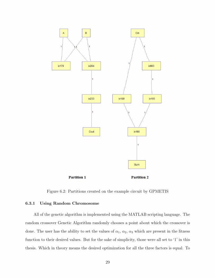
6.2 Partitions created on the example circuit by GPMETIS . . . . . . . . . . . . . . 29

6.3 Run-time of the traditional and new Methodologies with the size of the circuit . 31

A.1 An example Datagraph on which the functioning of GPMETIS is demonstrated 40

vi

List of Tables

6.1 Improvement over the fitness of various benchmarks after 500 Iterations . . . . . 32

6.2 Time taken to reach the maximum fitness of each circuit using the traditionaland the proposed methodologies . . . . . . . . . . . . . . . . . . . . . . . . . . . 33

vii

Chapter 1

Introduction

This chapter briefly explains the overall structure of the thesis and why this study

was undertaken. It specifies the importance of this study along with an introduction to

the methods carried out to implement it. It serves as a roadmap for the rest of the thesis

providing the reader with the basic information needed to understand it and also a platform

to navigate through it smoothly.

The last four decades have witnessed a phenomenal growth in the field of VLSI. It is

expected to grow further more with no signs of saturation in the near future. As a result of

this rapid development, the life of mankind became easy, simple and affordable but on the

other hand, the VLSI designers were hampered by more and more obstacles making their

lives problematic. With high-density VLSI chips, many issues such as difficulty to design,

increased design time, increased delay, more power consumption, more area and unfeasible

design costs arose [1]. This forced engineers to come up with new strategies to optimize

these factors.

Partitioning is a technique in which larger components are efficiently and logically broken

up into smaller interacting sub-components for easy and better handling [2]. It is one efficient

way to address the problems caused by high-density chips by exploiting the design trade-offs

to make the design more efficient. For the same reasons mentioned above, in the recent

years, partitioning has become an important and integral part of the physical design of a

VLSI system [3]. Industry and academia are continuously working to find better algorithms

and methodologies to break a large design into competent partitions. However, partitioning

of high-density chips is very challenging and a lot of effort and time needs to be put in to

arrive at a good partition. It has been shown in the past that the partitioning problem

1

is NP-hard [4] [5]. Hence it is always important to develop heuristic algorithms and new

methodologies, which arrive at a reasonable solution in a plausible amount of time. Even

though there were a few ways studied earlier, there are some disadvantages to them, which

are examined in more detail in Chapter 2.

1.1 Background and Motivation

As a result of vigorous study undertaken in the area of partitioning to cope with the

enormous technology scaling, new techniques and heuristic procedures have emerged for

better partitions. Out of these many proposed algorithms, genetic algorithms proved to be

very promising in the field of VLSI. These algorithms serve as a pivot around which this

thesis is constructed. Genetic algorithms are heuristic algorithms based on Charles Darwin’s

theory of evolution by natural selection. This algorithm was adopted into VLSI partitioning

a few decades ago [16]. It logically partitions the circuit represented by the dataflow graph

over a few iterations until we get the best partition or we run out of iterations. Although it

was shown that genetic algorithms serve well in obtaining a feasible solution for the VLSI

partitioning problem, it was also evident that the genetic algorithms’ run time increases

rapidly with the increase in the size of a VLSI circuit [6] [7]. It is very important to reduce

this run time, if we need to get the most out of the genetic algorithms’ usage. This problem

is contemplated in the thesis, which provides the motivation to come up with a better

methodology and to reduce the time taken by the genetic algorithm to arrive at the solution.

1.2 Problem Statement

In this thesis a new methodology is proposed for VLSI circuit partitioning using genetic

algorithms, which significantly decreases the overall run-time of the partitioning algorithm.

In the previous methods a randomly generated crossover point was used in the genetic

algorithms, which could potentially kill some useful genes, thus increasing the algorithm

run-time. Hence, in this thesis a new approach is proposed, where the chromosome for the

2

algorithm is logically chosen, which is circuit specific, using a graph-partitioning algorithm.

This routine, in the later parts of the thesis, is proved to be efficient and faster than the

existing methods.

1.3 Structure and Scope of the Thesis

This thesis presents a new technique to generate an efficient solution for the problem of

VLSI circuit partitioning in less time, using genetic algorithms. Circumstantial evidence and

explanation is also provided to reinforce the proposal. This also proposes a new kind of a

fitness function, which provides the user with the flexibility to choose the weighting of various

properties of the system. However, the advantage of this fitness function over the previously

used functions is not portrayed explicitly in the thesis. The entire thesis uses the 350nm

technology standard cell libraries from the TSMC ASIC design kit, to compare and contrast

the various aspects of the Benchmark circuit modules. The experiment uses a MATLAB

tool to code all the algorithms required for it, which are not included in the documentation.

However, the detailed description of the functioning of the code is included in the Appendix.

Detailed description of the third party partitioning software used in the experiment is also

included in the appendix. Genetic implementing the new methodology and also without

implementing the new methodology is also implemented using the MATLAB script and all

the comparisons are done based on the run-time of this code.

The rest of the thesis is organized as follows:

Chapter 2 provides us with information of the relevant work carried out by different

authors in this area. This chapter prepares a platform for the reader to understand the

thesis and gain the needed insight.

Chapter 3 gives a general introduction on the evolution algorithms and then the brief

overview of genetic algorithms explaining its emergence, significance, uses and its relevance

to the thesis. This chapter explains the very functioning of genetic algorithms and deals

3

with the key concepts needed to understand the thesis. This chapter also emphasizes the

fitness function used in the experiment.

Chapter 5 introduces the methodology with all the supportive figures and explanation.

This chapter provides essential insight to see how the technique works to produce efficient

results in the VLSI partitioning.

Chapter 6 provides the necessary evidence to prove the superiority of this methodology

over the previous algorithms. This chapter could be studied if all the experimentation results

are to be analyzed.

Chapter 7 gives the final conclusion and also addresses the future prospects of develop-

ment using this methodology. This also mentions about the possible work that could still be

carried out on this thesis to make it even better and also add to its contribution.

The report concludes with the bibliography containing all the references cited in this

manuscript. If even more detailed investigation is required, the report finally has an Ap-

pendix, which describes all the functional modules scripted in MATLAB and also the notes

on ‘GPMETIS’, which is a third party graph partitioning software, provided by Karypis Lab,

which is used to partition the graph.

4

Chapter 2

Literature Survey

This chapter deals with the previous study carried out in the field of genetic algorithms

and their use in the partitioning of VLSI circuits. It also emphasizes on hardware/software

codesign techniques developed in the past using genetic algorithms. The studies in the area

of hardware/software codesign widely inspired the present thesis and it would be a good

start to learn about them before jumping into the proposed methodology.

The basics of genetic algorithms are quite comprehensively covered by Goldberg, David.

E. et. al. [8]. Also, the importance of partitioning is mentioned in several articles in the

literature [9], [3], which justifies the importance of the current undertaken study. Traditional

Genetic Algorithms use a random point to do the crossover over the chromosomes. Even

though this involves only a few computations, this is nothing more than a random searching

with little direction provided by the ever-evolving chromosomes.

A number of theories have been provided previously, which try to improve the selection

of crossover points. One such technique is proposed by Zhi-Qiang Chen, Yuan-Fu Yin,

et. al [10], where the individual chromosomes are compared and the crossover operator,

is generated based on the difference between the individuals. But this kind of comparison

involves a complicated set of computations at every iteration which nullifies the effect for

more complex systems like in the case of VLSI partitioning. It is important to get a better

crossover point with minimal amount of computational complexity in order to deal with

the highly complicated VLSI circuits where the total number of iterations can go into the

thousands.

Another useful proposal to improve the total run time of the genetic algorithm was

given by Shiu Yin Yuen, Chi Kin Chow et.al [11] which incorporates more control on the

5

mutation operator and keeps track of the chromosomes to avoid revisiting. This method

indeed improves the run-time of the algorithm, but still hasn’t improved the search space.

If the algorithm runs into a chromosome which is revisited earlier, it simply discards that

chromosome and moves ahead, saving that computational time. While this method is still

effective, controlling the search space at a higher level removes a lot of unnecessary computa-

tion down the line. Also this method has a serious threat from the amount of data generated.

For example, if we select a population size of 16 and run the algorithm for 10000 times, the

database should be large enough to hold information on 16×1000 = 16000 chromosomes and

an efficient search algorithm on these 16000 chromosomes has to be done at every iteration

to check if the chromosome has been visited earlier. This study aims to find a more effective

solution for this problem.

In the work of Wu Jigang, Thambipillai Srikanthan et.al [12], efficient algorithms for the

partitioning of hardware and software are presented which considers only the improvement

of area while also improving the run-time of the algorithms and power of the system. It

is a known fact that reducing the area of a circuit, in most cases, also reduces the power

consumption (due to the reduction of the transmission losses on the connections). This could

mean that the cost of implementing such a system could be very expensive. In the modern

day where millions of a particular kind of IC’s are shipped every day, even a small fraction

of increase in the IC size could add up to significant costs. Hence, in the current study,

cost is also included in the fitness function which significantly boosts the effectiveness of this

methodology. If, in a particular experiment, the cost is to be avoided, its coefficient could be

simply made ‘0’ in the fitness function. The importance of genetic Algorithms in partitioning

was found very early and several modifications to it are proposed. However, most of them

[13] still lack the intelligent chromosome selection, which hinders their time savings.

The work of Peter Arato et al [14], shows the idea of partitioning using both genetic

algorithms and integer linear programming (ILP). Again, even in this, the traditional pro-

cedure is followed to choose the crossover point randomly. However, this work shows that

6

Genetic Algorithms are superior to ILP, as far as the run-time is concerned. This has a

considerable amount of motivation in carrying out the present study on Genetic Algorithms,

overcoming the limitations of its random crossover point selection.

7

Chapter 3

Brief Overview of Genetic Algorithms

This chapter introduces the concepts of Genetic Algorithm, giving necessary examples

and supporting information to get a better understanding of the core logic.

3.1 Overview of Evolutionary Algorithms

Most of the computation problems involving real world inputs are NP hard and arriving

at a clear solution might take impossible amounts of time. Fortunately, in these scenarios,

getting close to the optimum solution might be enough to get fruitful results. Hence, over

a period of time many heuristic algorithms and procedures have been proposed which take

a logical approach to arrive at a useful solution without actually searching the entire search

domain. Among these algorithms, a special class of algorithms called the evolutionary algo-

rithms [15] have gained popularity and were shown to provide very good heuristic solutions

within a small amount of time. They also have been quickly adopted in the various problems

of optimization, design, searching and machine learning. These algorithms have been proved

to be extremely effective in the optimization problems.

Over many years, scientists from across the world independently worked on algorithms

which were inspired from biological events and the natural evolution, like the technique

developed by a flock of birds to help each other to find food, the branching technique of blood

vessels in our body to transport blood faster to different parts of the body, etc, which gave rise

to the evolutionary algorithms. These are hence, mostly inspired by nature and are adopted

and tweaked slightly to suit our needs and fit into the problem at hand. The evolutionary

algorithms are more intelligent as they change their mechanism and procedure for arriving

at a solution constantly throughout the algorithm, rapidly progressing towards a suitable

8

solution. The main backbone of these evolutionary algorithms is an encoding mechanism,

the scheme by which a mathematical problem is described or coded to be implemented

in the algorithm and a fitness function, which is constantly measured and used to evolve

the algorithm. After their introduction, scientists were able to describe large numbers of

complicated problems to be solved using these algorithms and arrive at promising solutions.

A subset of these evolutionary algorithms is genetic algorithms, which were used extensively

in the recent past and hold a lot of potential to solve complicated problems.

3.2 Overview of Genetic Algorithms

Genetic algorithms [8] are a popular class of evolutionary algorithms, which were inspired

by Charles Darwin’s theory of natural evolution and his concept of “survival of the fittest

”. After it was shown that solutions of various complicated problems, such as optimization

problems including the traveling salesman problem, searching problems , learning problems,

scheduling problems, placing and routing problems, etc, could be obtained more efficiently

and faster, genetic algorithms gained a lot of popularity. Even after approximately 50 years

since its discovery by John Holland and his students [17], genetic algorithms still remain

as a popular choice for many optimization problems. This gives a little hint about the

potential of these algorithms. Unlike other algorithms, genetic algorithms are not completely

randomized in arriving at their approach, but also use some directed approach and have an

ability to do a multi-dimensional search. But still the randomization is kept intact hoping

to achieve the global maximum by introducing a ‘mutation’ operator. This unique feature of

genetic algorithms enables arriving at a more realistic solution than its other contemporary

algorithms, still keeping the overall run-time low.

The general pseudo code of genetic algorithms is given in Algorithm 1 at the end of this

section.

9

3.3 Genetic Algorithms Terminology

3.3.1 Chromosomes

Before we apply these algorithms to a given problem, a representation of solutions to

the problem must be developed which is understood by the computer. These representations

are called ‘chromosomes’. Each chromosome is made up of fields, which represent various

properties of a problem. These fields are called ‘genes’. The Genetic algorithm creates such

chromosomes randomly and tries to find a best chromosome which represents a solution to

the problem.

3.3.2 Crossover

The genetic algorithm attempts to produce better generations for every iteration. This

involves “crossing over” the chromosomes at a certain ‘crossover point’. This means that

some positions are selected on two or more chromosomes, called ‘parent chromosomes’, and

the genes at these positions are exchanged to produce the ‘child chromosomes’. The off-

spring thus produced thus have the genes of both the parents (properties of both the parent

chromosomes). This process is called ‘crossover’ or ‘reproduction’.

The crossover may not necessarily happen only once with each pair of chromosomes.

There are many ways in which the total number of times a pair of chromosomes are used for

reproduction is allocated. Two widely used method are ratioing and ranking [8].

• In ratioing, the reproduction rate of a chromosome is in proportion to its fitness. If

the chromosome has higher fitness, it reproduces and contributes to more offspring. In

this way, the algorithm may soon reach a set of population of fit individuals. To enable

this a concept called ‘Roulette Wheel’ is introduced. This is a genetic operator which,

based on However, this method has a downside. If the algorithm finds a dominant

individual early, it may suppress the chromosomes from reproducing and hence we

may reach only a local maximum.

10

• The alternate to the ratioing method is the ranking method, where the chromosomes

are sorted based on their fitness and a certain rank is given to them. They then

reproduc based on their rank. The individuals with higher rank have a higher proba-

bility of reproducing and the individuals with lower rank have a lower probability of

reproduction. For this, again, the ‘Roulette Wheel’ concept, slightly modified, is used.

A pictorial representation of crossover is depicted in Figure 3.1.

We can see in the figure that the offspring produced from the chromosomes share the

genes of both the parents to inherit new and unique characteristics.

Figure 3.1: Pictorial Representation of a Genetic Crossover

3.3.3 Mutation

Genetic algorithms are a kind of ‘Hill Climbing’ type of algorithm, which may sometimes

get stuck at a local maximum. Mutation, just like in Biology, is a random alteration of a

gene in a chromosome. This is injected into the chromosomes occasionally to make sure that

the solution we reach is not a local maximum but rather global maximum. It is also possible

that during the process of crossover, the chromosomes which are not selected for generating

the next population, may along with them, lose some important genes. This can completely

11

change the final solution or may delay the program in getting there. Hence to avoid this,

sometimes mutation is essential to inject useful genes (information) into the chromosome.

3.3.4 Fitness Function

A ‘Fitness Function’, in short, is a mathematical model which represents the ability

of a chromosome to survive within the specified environment. It is unique to every given

problem, tailor made to hold all the important properties of the system on which the genetic

algorithm is applied. The final solution can only be as good as the fitness function. More

on fitness functions and the function used in this study are explained in detail in chapter 4.

Data: Pseudo Code implementation of Genetic Algorithm

Result: The chromosome with highest fitness

begin

Generate Initial Population P(t) at t=0;

Evaluate Fitness, f(t), of each chromosome ∈ P(t);

while specified condition is not satisfied do

begin

t=t+1;

Select fit individuals Pnew (t) so that Pnew (t) ∈ P(t-1) ;

Crossover each chromosome ∈ Pnew (t) to produce offspring;

Evaluate Pnew (t);

P(t) = Pnew (t) ;

end

end

end

Algorithm 1: Pseudo Code for Genetic Algorithm

12

3.4 Advantages of Genetic Algorithms

Since the genetic algorithms were first invented in the 1960’s, their popularity has been

increasing as they posses a lot of advantages compared to similar algorithms. Some of the

advantages are

• As long as we can encode system traits into a fitness function and represent the prop-

erties in the form of a chromosome, any complex problem can be solved using genetic

algorithms.

• Besides condensing down a large search space significantly, we can search within a it

relatively quickly when compared to other algorithms. This is because these algorithms

use a unique strategy by which a wide variety of points in a search space are selected

and a directed search through that space is performed, gradually converging towards

the optimum solution [8].

• Genetic algorithms are a hill-climbing type of algorithm. Unlike other hill-climbing

algorithms, genetic algorithms do not get stuck at the local optima values due to

the occasional mutation operation. Even though they take fractionally more time in

reaching the solution due to this operation, they make sure that the final output is a

global optimum and not local optima.

• The other important advantage of genetic algorithms is that the problem search space

need not be continuous. Even if it is discretely defined, the intermediate solutions

undergo genetic crossover and produce better solutions (solutions which are originally

not defined in the search space). Hence these algorithms makes really important con-

tributions to solving problems where only little amount of data is known relating to

the search space.

• As the genetic algorithms can be controlled by the user and he decides when to ter-

minate the flow, if configured properly, they could be very effective in problems which

13

have more than one solution. If a problem has more than one solution and we continue

to run the algorithm even after finding the first solution, the algorithm may continue

to find the next solution as well.

The graph of fitness function vs. number of iterations, while running the Genetic Algo-

rithm over a few iterations, is presented in figure3.2.

Figure 3.2: The fitness vs. the total number of iterations of a Genetic Algorithm

14

Chapter 4

Overview of the Fitness Function used in the Methodology

As mentioned earlier, a fitness function is generally a mathematical description, used to

evaluate the fitness of a chromosome as a candidate solution to a particular problem. The

fitness function should hold in it all the important traits of a system, which are desired to be

optimized. In other words, a fitness function is the sole measure with which the algorithm

decides to accept or reject a chromosome. There are a few main characteristics of a fitness

function, which should be considered for effective implementation of the algorithm. Among

these, the two essential features in selecting a fitness function are:

• It should be compact, yet completely representing the desired traits of a system so as

to make sure that the chromosomes selected based on this fitness function represent

the close to optimum implementation of the circuit.

• It should be computationally small, i.e., it should take minimal amount of time to be

computed. As a fitness function is evaluated for every chromosome for every generation;

more complex fitness functions lead to genetic algorithms with long run-time.

In this thesis, the problem in front of us is to find an effective solution for circuit partitioning,

with the circuit characteristics like area, cost and delay to be as minimized as possible.

Keeping this in mind, essentially, we need to find a circuit implementation that has a low

value of area, cost and delay. Hence the fitness function given below is framed keeping in

mind the important characteristics for a good fitness function mentioned earlier.

f = α1(area) + α2(cost) + α3(delay) (4.1)

15

In the above equation, α1, α2, α3 are positive numbers which the user chooses as per

the requirement. Assuming the area, cost and delay to be mere integers, equation 4.1 is

reasonably compact, describes the problem almost exhaustively as it contains the variables

of interest like the area, cost and the delay and also, as it is a simple linear mathematical

equation with no complicated operators, it is computationally efficient and thus ensures that

the range of f is bounded. Consider we send a chromosome “110010100” to this function,

where ‘1’ represents a particular kind of implementation and ‘0’ represents a different kind of

implementation. Based on the chromosome, the fitness function calculates the total area of

the circuit, worst-case delay from input to output across the partitions, and the total costs

for this implementation, including the communication costs. Hence this fitness function

can be used effectively to tackle the problem at hand and produce the necessary optimized

solution. Many real time problems might have more than two kinds of implementations. In

such scenarios, the chromosome encoding can be undertaken in a more complicated fashion,

as per the requirements. Even then, the overall functioning would be the same.

When we run the genetic algorithm, every time a generation passes, the fitness of the

current population is measured. The algorithm runs until the required fitness is obtained or

we run out of iterations. In the above equation, the main traits are area, cost and delay. In a

given system, these traits would be always desired to be as minimum as possible and hence,

the chromosome with the least value of f is said to be the best solution or the chromosome

with the best fitness.

The fitness function also provides the user with three coefficients, α1, α2 and α3 to

the individual variables of the fitness function, which allows the user to manually set the

priorities. For example, if the user can afford to spend some money on the design to get

more area-optimized circuit, he or she can increase the weight of the area variable (α1) and

decrease the weight of the cost (α2). Obviously, if all the coefficients are of equal weight,

then all the three factors are optimized equally.

16

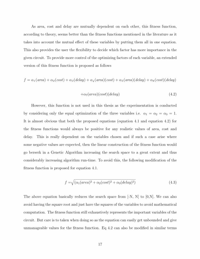
As area, cost and delay are mutually dependent on each other, this fitness function,

according to theory, seems better than the fitness functions mentioned in the literature as it

takes into account the mutual effect of these variables by putting them all in one equation.

This also provides the user the flexibility to decide which factor has more importance in the

given circuit. To provide more control of the optimizing factors of each variable, an extended

version of this fitness function is proposed as follows

f = α1 (area) + α2 (cost) + α3 (delay) + α4 (area)(cost) + α5 (area)(delay) + α6 (cost)(delay)

+α7(area)(cost)(delay) (4.2)

However, this function is not used in this thesis as the experimentation is conducted

by considering only the equal optimization of the three variables i.e. α1 = α2 = α3 = 1.

It is almost obvious that both the proposed equations (equation 4.1 and equation 4.2) for

the fitness functions would always be positive for any realistic values of area, cost and

delay. This is really dependent on the variables chosen and if such a case arise where

some negative values are expected, then the linear construction of the fitness function would

go berserk in a Genetic Algorithm increasing the search space to a great extent and thus

considerably increasing algorithm run-time. To avoid this, the following modification of the

fitness function is proposed for equation 4.1.

f =√

(α1(area)2 + α2(cost)2 + α3(delay)2) (4.3)

The above equation basically reduces the search space from [-N, N] to [0,N]. We can also

avoid having the square root and just have the squares of the variables to avoid mathematical

computation. The fitness function still exhaustively represents the important variables of the

circuit. But care is to taken when doing so as the equation can easily get unbounded and give

unmanageable values for the fitness function. Eq 4.2 can also be modified in similar terms

17

to avoid the negative values There are also similar modifications available in the literature

to handle the negative values like “Power Law Scaling” and “Sigma Truncation” but these

are completely out of the scope of the thesis.

The main missing element in the present fitness function is the power variable which

in these days have gained a lot of prominence. However, as power is not a straight forward

metric available for most of the circuits, to avoid complexity it has been ignored in the thesis.

Also, we need to keep in mind that we need to run the algorithm for many iterations and

calculating power for every iteration may not be within the scope of this thesis and is left

over for future considerations.

18

Chapter 5

Overview of the Methodology

As shown in the in Figure 5.1, the traditional genetic algorithms in the literature will

choose the crossover points randomly. With this method, the algorithm just jumps into the

search space without a proper direction, searching for candidate solution which best match

the fitness function. This significantly delays the overall run-time of the algorithm. Contrary

to this, in this thesis a new methodology is proposed where a circuit-specific crossover point

is intelligently chosen based on the partitions generated by the graph partitioning algorithm.

This provides a direction to the algorithm to start the search in the search space, which

otherwise is significantly large, giving rise to faster and efficient solutions.

5.1 Methodology

To begin with, the circuit description is taken and is converted into a datagraph repre-

sentation using a parser code. This datagraph is given as an input to a graph partitioning

algorithm which partitions the circuit into two parts (or more parts based on the require-

ment). This partition would later act as the crossover point in the algorithm. The circuit is

partitioned based on two factors.

• The number of edges across the partition are as low as possible

• The number of nodes on either side of the partition as balanced as possible.

• The communication costs between the two partitions are minimized.

Each node of the datagraph representation of the circuit is randomly assigned a value of

either ‘0’ or ‘1’ according to their respective implementation. This array of bits containing 1’s

19

Figure 5.1: Traditional Partitioning Flowchart

and 0’s, which correspond to the properties of each node in the datagraph, constitute to one

‘chromosome’ (which also might be called as individuals, phenotype, genotype or creatures).

Each bit in this chromosome representing the kind of implementation of that paticular node

is called the ‘gene’ of the chromosome. The size of each chromosome is ‘V’, where ‘V’ equals

the total number of nodes in the datagraph (which is equal to the total number of gates in

the circuit). Hence in short, we can say, for a given circuit containing ‘V’ number of gates,

each chromosome has ‘V’ number of genes. A fixed number of such random chromosomes

are created and grouped which construct the ‘initial population’. The datagraph is fed to

the graph-partitioning algorithm, which partitions it into two parts. We can also partition

20

the graph into smaller parts enabling faster running algorithms, but this study is setup only

to handle only 2 partitions. This partition represents the crossover point of our genetic

algorithm. The user selects the properties intended to be optimized in the fitness function

and each chromosome in the initial population is fed to the fitness function to calculate their

corresponding fitness. The chromosomes with low fitness are discarded and those with high

fitness are chosen for the reproduction of next generation of the offspring. The fitness of the

thus created ‘new population’ along with the initial population is calculated and again the

chromosomes with low fitness are discarded and chromosomes with high fitness are crossed

over, based on the crossover point generated by the graph partitioning algorithm,to produce

new population. This process continues and a database is created within the algorithm to

store the fitness of each chromosome after every generation. We stop the algorithm when we

find a chromosome with maximum fitness or we run out of the total number of generation

cycles (i.e the total number of iterations specified by the user). The flowchart of this new

proposed methodology is depicted in figure 5.3.

Figure 5.2: Idea of partitioning - final solution

The algorithm spits out a final chromosome, which has the best fitness and thus rep-

resents the best implementation of the circuit at hand. The genes in this chromosome are

21

then decoded and the kind of implementation of each node in the circuit is figured out (If

the gene representing a node is 0, we implement in the 1st style of implementation and if

it is 1, we implement it using second style of implementation). The final solution of an

example circuit looks something like in figure 5.2. As shown in this figure, different gates

of the design, implemented in different styles, co-exist and hence this kind of design is also

called as co-design. We can hope to have this kind of co-design to have the maximum fitness

and thus the most efficient way to implement the logic to get our desired results.

Figure 5.3: Proposed Paritioning Methodology Flowchart

22

To increase the search space and to obtain a global maximum instead of a local max-

imum, the chromosomes occasionally undergo ‘mutation’, which is a process of randomly

altering a gene based on a defined condition. In this methodology, in order to undergo mu-

tation, a gene is randomly selected in the chromosome and its bit is inversed. However, care

should be taken to keep the probability of mutation optimum. Greater the probability of

mutation, greater the time taken to reach the optimum value and better is its quality. But,

as is with everything, even the mutation probability also has a limit. Increasing the mutation

probability increases a lot of chaos in the algorithm which converts the Genetic Algorithm

into a mere randomly searching algorithm. Generally, in this experiment, the probability of

mutation is in the order of 0.001, i.e out of every 1000 chromosomes, one chromosome would

be mutated. But this probability could completely be changed in other problems depending

upon the type of solution required and other parameters.

23

Chapter 6

Implementation and Results

This chapter in details discusses how the proposed methodology is implemented in this

thesis. It also gives a through explanation of supporting functional code and algorithms used

to get a close to accurate results. The chapter also gives evidence to support the conclusions.

6.1 The input files and data used by the methodology

The RTL description of the circuit of interest is taken and synthesized using Mentor

Graphic’s Leonardo Spectrum [18]. This produces a .vhd netlist of the circuits using the

standard gates defined in the TSMC ASIC design kit. The technology of the gates using

which the netlist is built is of 350nm. The goal of the thesis is to implement a part of our

circuit in this technology. All the gates implemented in this technology are given a logic

value ‘1’. More information is given as to how this value is used in given in the later part

of the chapter. For the second kind of implementation, an FPGA board is taken where the

gates are implemented in a similar technology of 350nm as it is essential to have both the

implementations in the same technology for a reasonable comparison. For this the FPGA

board chosen is the Xilinx Cool-Runner CPLD board (XA9500XL). The part of the circuit

implemented in this technology is treated as our second implementation and all the gates

which use this technology are given a logic ‘0’.

It is a know fact, that implementing a circuit in an FPGA increases the area of the

circuit, decreases the speed of operation but is cost efficient. Similarly implementing the

circuit in a standard-cell based approach increases the cost of the design but drastically

improves the performance of the design. Hence it would be wise to implement the critical

parts of the circuit which are important in determining the speed using a faster technology

24

without caring about the implementation cost and using the FPGAs to implement the not

so critical paths of the design. When the design complexity is extremely high, it is almost

impossible for us to manually differentiate the design into the two kinds of implementations.

Hence, there were many algorithms which emerged to do this task for us. The front runner

among all the algorithms are those which effectively use the genetic algorithms. That been

said, as the complexity of the designs increase rapidly every year, the need for more effective

algorithms is also exponentially increasing. That’s where this new methodology plays a

prominent role. Hence the main objective of this study is to find an efficient method to

partition the circuit into two parts, such that the total cost of implementation is as low as

possible and also, the total area of the design, the total critical delay of the design are as

low as possible.

6.2 Parser

The two main functions of the parser code in this experiment are

• To construct a datagraph based on the .vhd netlist provided by the Leonardo Spectrum

and

• To format the circuit into a .graph representation which would be used by ‘gpmetis’

which is an open source graph partitioning software.

6.2.1 Contructing a Datagraph

The .vhd netlist generated by the Leonardo Spectrum is fed to the parser program.

This, based on the important labels and keywords of VHDL languages extracts the key

information like the total number of gates, inputs and outputs the the gate, total number of

edges (i.e the wire connections between the gates) and the type of the gate.

The .vhd netlist of a simple supporting circuit is shown below.

25

The netlist shown above is understood by the parser algorithm, which reconstructs it

back into the data graph format, where the connection between the two gates is represented

by the a single line. So each gate in the circuit is represented as a node in the datagraph

depiction. It should be noted that to make the algorithm simpler, the inputs and outputs

of each circuit are represented as a node which gives a handle for the Genetic algorithm to

work on all nodes between them. To clearly show the functioning of the parser code, a .vhd

netlist of a simple circuit is taken, which is sent as an input to the the parser block.

In the example .vhd netlist above generated by the Leonardo Spectrum, the parser code

recognizes the instances of gates based on the label after the ‘begin’ VHDL keyword. It

makes an array of all the instance of various gates and associates the gate type for each

instance. It also recognizes the connection between each gate to the other gates, based on

26

Figure 6.1: Datagraph Representation of a circuit created by the Parser Program

the inputs and outputs to each gate. All this data is used to reconstruct the circuit into a

data graph format. The circuit’s datagraph representation is shown in Figure 6.1.

In the Figure 6.1, we can also observe that the inputs and outputs, which are ‘A’, ‘B’,

‘C ′in and ‘Sum’, ‘C ′

out respectively are also denoted as nodes in the datagraph. However, the

27

algorithm is intelligent enough to consider this ambiguity and not assign any 1’s or 0’s to

them in the process.

6.2.2 Partitioning the Graph using GPMETIS

GPMETIS is an open source graph partitioning software which takes the circuit descrip-

tion in a .graph format file which is just a bunch of numbers representing the circuit and the

connections. Detailed information of the functioning of GPMETIS is not in the scope of the

thesis and interested readers, if interested, can get more information of it in notes provided

about it in Appendix I. The GPMETIS gives out a stream of 0’s and 1’s representing the

two partitions in which the circuit is split. It should be noted that this convention of 0’s

and 1’s are completely the software’s way of representing that two partitions and it is in now

way related to the genes of chromosomes used in this study.

The parser, then takes back the output of GPMETIS and identifies the chromosome

which is fed to the Genetic Algorithm code, which would be explained in detailed in the

subsequent sections. To help visualize the partition, the outputs of the GPMETIS are used

to construct a sparse matrix which is used to graphically show the partitions using MATLAB

tool. The datagraph in figure 6.1 is split into two partitions by the GPMETIS software which

is shown in the figure6.2

6.3 Genetic Algorithm Program

Using this code, we actually implement the Genetic Algorithm. To differentiate the old

and new methodologies, the Genetic Algorithm code is slightly modified in two ways.

• One way is to randomly create the crossover point within the algorithm and thus

implementing the traditional methodology shown in figure 5.1.

• The other way is to take the partition created by the GPMETIS and use it as the

crossover point which reflects the new methodology shown in figure 5.3.

28

Figure 6.2: Partitions created on the example circuit by GPMETIS

6.3.1 Using Random Chromosome

All of the genetic algorithm is implemented using the MATLAB scripting language. The

random crossover Genetic Algorithm randomly chooses a point about which the crossover is

done. The user has the ability to set the values of α1, α2, α3 which are present in the fitness

function to their desired values. But for the sake of simplicity, those were all set to ‘1’ in this

thesis. Which in theory means the desired optimization for all the three factors is equal. To

29

provide with the values for area, cost and delay, it would be wise to use a database which

readily provides the data when requested, instead of simulating every time for those values.

This would decrease the accuracy to some extent, but it is very reasonable when compared

to the quality of the final chromosomes. This data is provided by a “library file” which is

provided as an input to the genetic algorithm. This file contains the important data of the

gates which are necessary to calculate the fitness for every iteration. The library file also

contains the information of the propagation delay of each gate. However, the performance

of a circuit depends on a critical path of the design. When, for every iteration, we keep

changing the style of implementation, the critical path may vary. Hence another supporting

functional code which discovers the slowest path in the design for every iteration is used.

Care is taken that this code acts as fast as possible. However, it should be noted that this

piece of software only gives the path which takes the highest propagation time, but does

have the intelligence to check if it is the ‘false path’.

6.3.2 Using Circuit Specific Chromosome

To implement the proposed methodology, the Genetic Algorithm is programmed to take

the chromosome fed to it by the parser, instead of generating a random crossover point. There

is a small time overhead in this methodology due to the calculation of the circuit specific

crossover point which is not present in the traditional genetic algorithm. However, this time

overhead is very small and is insignificant for large circuits. The fitness function, the library

file, the fitness function coefficients and the delay calculation code would remain the same

even in this methodology. The only thing that changes is the way it gets the crossover point.

Maintaining this consistency is essential to make a proper comaparision between the new

methodology and the existing traditional methodologies.

The time overhead between the new methodology and traditional methodology is de-

picted in the figure 6.3.

30

Figure 6.3: Run-time of the traditional and new Methodologies with the size of the circuit

The variable TD in the figure 6.3 denotes the time overhead of the new methodology.

After repeated experimentation, it was found that this time overhead is significant for circuits

which have a value of ND of around 100 to 150 gates. In any circuit which has more than

this 150 gates, this time overhead is insignificant and the proposed methodology gives more

efficient results. In today’s time, where we talk about circuits with millions of gates, a

circuit with less than 150 gates is almost obsolete or even if they are to be optimized, we

can manually achieve very good results rather than using an algorithm. Hence, the time

overhead associated with the new methodology stand as a no threat to get efficient results.

6.4 Results

The new methodology proposed is implemented on various benchmark circuits, using

the functional codes mentioned in the earlier sections. The benchmarks used are S713,

S13207, S15850, S35932, S38417, S38584 [19]. This implementation is also compared to the

traditional implementation and the difference is contrasted in the results provided in the

following sections of the document.

31

In the table 6.1 the traditional Genetic Algorithm Methodology and the new proposed

methodology are run on various benchmark circuits for 500 iterations and the time taken for

each of the methodologies is calculated. Also the percentage of improvement caused by the

new methodology over the old methodology is also provided in the last column of the table.

From these results there are 2 important points which are to be noted.

• The first thing to note is that the benchmark S713, which has only 170 gates, has not

shown any improvement in the final fitness when implemented in both the methodolo-

gies.

This could be because the S713 was small enough to achieve its highest fitness before

500 iterations for both the methodologies or because the time over-head for calulating the

crossover point in the new methodology dominated the total run-time. Whichever might

be the reason, would be more clear in the subsequent evidence to be presented later in this

manuscript.

• The second thing to note is that the percentage of total improvement in the fitness

increases with the increase in total number of gates.

Which means that the new methodology is more effective for larger circuits than the

smaller circuits. Hence with large circuits we obtain more savings.

BenchmarksCircuit

Number ofgates

Fitness after 500iterations usingold methodology

Fitness after 500iterations using new

methodology

% of improvement

S713 170 824 824 0S13207 3672 8712 9508 11.8S15850 4945 11844 13385 13.01S35932 15543 201019 274830 36.72S38417 13473 180792 242150 33.94S38584 13328 180111 239330 32.88

Table 6.1: Improvement over the fitness of various benchmarks after 500 Iterations

32

The overall repetitions of the Genetic Algorithm can be stopped in two ways. One would

be to stop the algorithm when we reach the maximum or intended fitness or the other way

is to let the algorithm run for a fixed number of iteration and select the chromosome with

the maximum fitness. The former method would be useful when we have some knowledge

about the circuit and what a good implementation might be. If we don’t know anything

about the circuit, it would be better to follow the latter method by allowing the algorithm to

run for some specified number of iterations based on the processing capability and available

resources.

Hence to compare the new methodology and the traditional methodology by the time

taken by them to reach the maximum fitness of each bechmark circuit is also gathered and

are presented in Table 6.2.

BenchmarckCircuit

Number ofgates

Time to reachmaximum fitnessusing traditional

methodology

Time to reachmaximum fitnessusing proposedmethodology

% ofimprovement

S713 170 74 78 -5.18S13207 3672 2097 1797 16.7S15850 4945 2416 2058 17.4S35932 15543 10285 7253 36.72S38417 13473 7625 5493 33.94S38584 13328 7588 5455 32.88

Table 6.2: Time taken to reach the maximum fitness of each circuit using the traditionaland the proposed methodologies

Again in the table 6.2, we can observe that for the benchmark circuit S713, the per-

centage of improvement in the total time to achieve the maximum fitness is negative. This

negative time indicates the time overhead, which is necessary for the calculation of the

crossover point by the graph partitioning algorithm.

Various data available in this section of the thesis and the details of the implementation

methodology discussed earlier stands as a strong evidence to show the effectiveness of the

new methodology. The output of the Genetic Algorithm is a stream of 1’s and 0’s whose

33

length is equal to the total number of gates in that circuit. Which means the largest circuit

in the chosen benchmarks, S35932, when fed into the genetic algorithm, produces a 15543

bits of binary value. This represents the most fit chromosome and gives a suggestion as to

how to implement the circuit in order to have the combined least value of area, cost and

delay.

34

Chapter 7

Conclusion and Future Work

As it has been shown in this new methodology that when the genetic algorithm is given

a little push by intelligently choosing the crossover point, it gives us more efficient results

faster. Unlike the traditional partitioning methods using genetic algorithms, where the

searching operation starts and proceeds randomly, in this method a little bit of processing is

performed on the circuit at hand, to figure out a logical point to start the algorithm. This

reduces a lot of work for the genetic algorithm and thus saving significant amount of time. In

today’s applications, where the size of VLSI circuits is becoming exponentially large, the rise

time of these algorithms are also increasing along with them. We have reached a point where

traditional algorithms would give acceptable results only in unfeasible amounts of time. This

is where this new method plays a prominent role. As shown in tables 6.1 and 6.2, the fitness

and run-time have been improved for about 50% for a circuit of size 15000 gates and the

curve only rises higher for larger circuits. In today’s practical applications, the gate sizes are

much more than these and hence we can expect much larger improvements in the quality

of the solutions and also the time taken to reach them. The user also has the opportunity

to alter the process in which this algorithm is implemented. In this methodology, due to

the contribution of the adaptive fitness function, the user has complete control over the

quality of the solutions. The user can also increase the accuracy of data residing within the

library file to get better results. Highly accurate data within the library file only means more

accurate data without any timing penalty. With these features, this methodology serves to

be a powerful tool in achieving quality circuit partitions. As this proposal only serves as a

skeleton for much sophisticated and custom built applications, the scope of areas, in which it

could be effectively applied is also vast. As, the technologies in which the modern day VLSI

35

circuits are changing very rapidly, to get accurate time to time information, the user should

just update the library file to get the best results. Which means, the same methodology can

be applied for outdated technology nodes or the current state-of-the-art technology nodes

by just providing the appropriate data to the algorithm through the library file. This makes

the methodology more robust and more flexible.

This methodology gets even more effective if more traits that determine the quality of

a design are incorporated into the design. One immediate suggestion would be to add the

‘power’ variable. It would be great if the fitness function can somehow hold the variable

representing the power consumption of the design. This could be a little tricky as the power

consumption of the design cannot be readily fed to the algorithm using a library file. Every

time the way of implementation of the gates change, we need to simulate the entire circuit

with the new composition. As we know power simulation itself is a very time taking process,

simulating a circuit for every iteration is close to impossible. Hopefully some better ways to

go around this obstacle would be put forward in the future, thus complementing the potential

of this methodology to a greater extent.

Other areas, which could be good to ponder are developing a kind of more adaptive

fitness functions, which are custom made to the circuit the methodology is dealing with.

Even though this idea is just suggested as another area to explore, this undertaken study

does not provide much information in this direction.

36

Bibliography

[1] Fortes, J. A B, ”Future challenges in VLSI system design,” VLSI, 2003. Proceedings.IEEE Computer Society Annual Symposium on , vol., no., pp.5,7, 20-21 Feb. 2003

[2] Shanavas, I.H.; Gnanamurthy, R.K.; Thangaraj, T.S., ”A Novel Approach to Find theBest Fit for VLSI Partitioning - Physical Design,” Advances in Recent Technologies inCommunication and Computing (ARTCom), 2010 International Conference on , vol.,no., pp.330,332, 16-17 Oct. 2010

[3] Frank M. Johannes. 1996. “Partitioning of VLSI circuits and systems”. In Proceedingsof the 33rd annual Design Automation Conference (DAC ’96). ACM, New York, NY,USA, 83-87.

[4] Saeednia, S., ”New NP-complete partition problems,” Information Theory, IEEE Trans-actions on , vol.48, no.7, pp.2092,2094, Jul 2002

[5] Sen, A.; Deng, H.; Guha, S., ”On a graph partitioning problem with applications toVLSI layout,” Circuits and Systems, 1991., IEEE International Sympoisum on , vol.,no., pp.2846,2849 vol.5, 11-14 Jun 1991

[6] Thang Nguyen Bui; Byung-Ro Moon, ”Genetic algorithm and graph partitioning,”Computers, IEEE Transactions on , vol.45, no.7, pp.841,855, Jul 1996

[7] Hidalgo, J.I.; Lanchares, J., ”Functional partitioning for hardware-software codesignusing genetic algorithms,” EUROMICRO 97. New Frontiers of Information Technology.,Proceedings of the 23rd EUROMICRO Conference , vol., no., pp.631,638, 1-4 Sept. 1997

[8] Goldberg, David E.,“Genetic Algorithms in Search, Optimization and MachineLearning”,first edition, Addison-Wesley Longman Publishing Co., Inc, 1989,Boston,MA,USA.

[9] sao-jie chen, chung-kuan cheng, “ Tutorial on VLSI Partitioning”, “VLSI Design”, Over-seas Publisherse Association, Published by license under the Gordon and Breach SciencePublishers Imprint, 2000, Malaysia.

[10] Zhi-Qiang Chen; Yuan-Fu Yin, “An new crossover operator for real-coded genetic algo-rithm with selective breeding based on difference between individuals”, Natural Com-putation (ICNC), 2012 Eighth International Conference on , vol., no., pp.644,648, 29-31May 2012.

37

[11] Shiu-Yin Yuen; Chi Kin Chow, “A Genetic Algorithm That Adaptively Mutates andNever Revisits”, Evolutionary Computation, IEEE Transactions on , vol.13, no.2,pp.454,472, April 2009

[12] Wu Jigang; Srikanthan, T., “Efficient Algorithms for Hardware/Software Partitioningto Minimize Hardware Area”, Circuits and Systems, 2006. APCCAS 2006. IEEE AsiaPacific Conference on , vol., no., pp.1875,1878, 4-7 Dec. 2006

[13] Prof. Sharadindu Roy, Prof. Samar Sen Sarma, “Improvement of the quality of VLSIcircuite partitioning problem using Genetic Algorithm”, Journalof Global Research inComputer Science, December 2012.

[14] Arato, P.; Juhasz, S.; Mann, Z.A.; Orban, A.; Papp, D., ”Hardware-software partition-ing in embedded system design,” Intelligent Signal Processing, 2003 IEEE InternationalSymposium on , vol., no., pp.197,202, 4-6 Sept. 2003

[15] Lawrence David Davis, Kenneth De Jong, Micheal D. Vose, L. Darell Whitley, “Evolu-tionary Algorithms - The IMA Volumes in Mathematics and its Applications (vol 111)”,first edition, Springer, June 4 1999.

[16] C. M. Fiduccia, R. M. Mattheyses, “A linear-time heuristic for improving networkpartitions”,Proceedings of the 19th Design Automation Conference, IEEE Press, 1982.

[17] John H. Holland, “Adaptation in natural and artificial systems”, MIT Press, 1992.

[18] Leonardo Spectrum, Mentor Graphics Corporation, available athttp://www.mentor.com/products/fpga/synthesis/leonardo spectrum/ , 2003.

[19] ISCAS’89 and ’85 Benchmark Information, CAD Benchmarking Lab, NCSU, availableat http: //www.cbl.ncsu.edu/www/CBLDocs, 1989.

38

Appendix A

Notes on GPMETIS

The GPMETIS is a software module which is a subset of a more sophisticated softwarecalled METIS1 developed by Dr. George Karypis et.al at the University of Minnesota.Apparently METIS is a “set of serial programs for partitioning graphs, partitioning finiteelement meshes, and producing fill reducing orderings for sparse matrices. The algorithmsimplemented in METIS are based on the multilevel recursive-bisection, multilevel k-way, andmulti-constraint partitioning schemes. ”.

A.1 Input File Format to the software

METIS defines a file format called as ‘.graph’ which numerically holds the informationabout a graph to be partitioned.

The primary input of the partitioning and fill-reducing ordering programs in METISis the undirected graph to be partitioned or ordered. This graph is stored in a file and issupplied to the various programs as one of the command line parameters. A graph G =(V,E) with n vertices and m edges is stored in a plain text file that contains n + 1 lines(excluding comment lines). The first line, referred to as the header line contains informationabout the size and the type of the graph, while the remaining n lines contain informationfor each vertex of G. Any line that starts with line and is skipped. The header line containseither two (n, m), three (n, m, fmt), or four (n, m, fmt, ncon) parameters. The first twoparameters (n, m) are the number of vertices and the number of edges, respectively. Notethat in determining the number of edges m, an edge between any pair of vertices v and u iscounted only once and not twice (i.e., we do not count the edge (v, u) separately from (u,v)). For example, the graph in Figure 2 contains 11 vertices. The fmt parameter is usedto specify if the graph file contains information about vertex sizes, vertex weights, and edgeweights. The fmt parameter is a three-digit binary number. If the least significant bit is setto 1 (i.e., the 1st bit from right to left), then the graph file provides information about theweights of the edges. If the second least significant bit is set to 1 (i.e., the 2nd bit from rightto left), then the graph file provides information about the weights of the vertices. Finally, ifthe third lest significant bit is set to 1 (i.e., the 3rd bit from right to left), then the graph fileprovides information of the sizes of the vertices. For example, if fmt is 011, then the graphfile provides information about both vertex weights and edge weights. Note that when thefmt parameter is not provided, it is assumed that the vertex sizes, vertex weights, and edgeweights are all equal to 1.

1METIS stable version: 5.1.0, 3/30/2013; MT-METIS initial version: 0.1, 5/21/2013

39

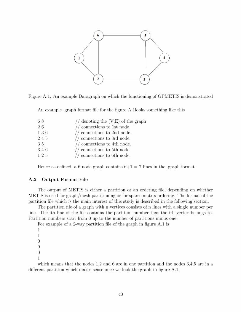
Figure A.1: An example Datagraph on which the functioning of GPMETIS is demonstrated

An example .graph format file for the figure A.1looks something like this

6 8 // denoting the (V,E) of the graph2 6 // connections to 1st node.1 3 6 // connections to 2nd node.2 4 5 // connections to 3rd node.3 5 // connections to 4th node.3 4 6 // connections to 5th node.1 2 5 // connections to 6th node.

Hence as defined, a 6 node graph contains 6+1 = 7 lines in the .graph format.

A.2 Output Format File

The output of METIS is either a partition or an ordering file, depending on whetherMETIS is used for graph/mesh partitioning or for sparse matrix ordering. The format of thepartition file which is the main interest of this study is described in the following section.

The partition file of a graph with n vertices consists of n lines with a single number perline. The ith line of the file contains the partition number that the ith vertex belongs to.Partition numbers start from 0 up to the number of partitions minus one.

For example of a 2-way partition file of the graph in figure A.1 is110001which means that the nodes 1,2 and 6 are in one partition and the nodes 3,4,5 are in a

different partition which makes sense once we look the graph in figure A.1.

40