An Early Warning Model of Bank Failure in Jamaica: An Information Theoretic Approach Jide Lewis 1 Financial Stability Department Research and Economic Programming Division Bank of Jamaica Abstract In this paper, an early-warning bank failure model (EWM) is designed to capture the dynamic process underlying the transition of the banks from financial sound to closure utilizing a transition probability matrix (TMP). Specifically, Instrumental Variables- Generalized Maximum Entropy (GME-IV) formalism by Golan et al. (1996) is used to assess the likelihood of the banking sector experiencing distress via the evaluation of banking crisis probabilities. The framework is also used to assess the impact of hypothetical but plausible macroeconomic and bank-specific shocks on the stability of the commercial banking sector over the medium-term. The informational approach performs well even when data are limited, ill-conditioned, or when explanatory variables are highly correlated, making it an appropriate framework for the evaluation of bank- failure dynamics. JEL Classification: C13, C14, C25, C51, C21 Keywords: Bank Failure, Early Warning Model, Markov Process, Generalized Maximum Entropy Estimators Author E-Mail Address: [email protected]1 The views expressed in this paper are those of the author and do not necessarily reflect the view of the Bank of Jamaica.
Transcript
An Early Warning Model of Bank Failure in Jamaica: An
Information Theoretic Approach
Jide Lewis1
Financial Stability Department Research and Economic Programming Division
Bank of Jamaica
Abstract In this paper, an early-warning bank failure model (EWM) is designed to capture the dynamic process underlying the transition of the banks from financial sound to closure utilizing a transition probability matrix (TMP). Specifically, Instrumental Variables-Generalized Maximum Entropy (GME-IV) formalism by Golan et al. (1996) is used to assess the likelihood of the banking sector experiencing distress via the evaluation of banking crisis probabilities. The framework is also used to assess the impact of hypothetical but plausible macroeconomic and bank-specific shocks on the stability of the commercial banking sector over the medium-term. The informational approach performs well even when data are limited, ill-conditioned, or when explanatory variables are highly correlated, making it an appropriate framework for the evaluation of bank-failure dynamics. JEL Classification: C13, C14, C25, C51, C21 Keywords: Bank Failure, Early Warning Model, Markov Process, Generalized Maximum Entropy Estimators Author E-Mail Address: [email protected]
1 The views expressed in this paper are those of the author and do not necessarily reflect the view of the Bank of Jamaica.
2
TABLE OF CONTENTS
I. Introduction ………………………………………………………… 3 II. Literature Review …………………… …………………………... 4
III. Data………………………………………………………………….. 8
IV. Methodology……………………………………………………...... 11
i. A Markov Transition Model Early Warning System……… 11
ii. Diagnostics and Model Reliability………………………..… 16
V. Empirical Results …………………………………………………. 18
VI. Conclusions …………….…………………………………………... 25
References 26
3
I. Introduction The last two decades have seen a proliferation of systemic banking crises, as documented
by the studies of Lindgren, Garcia, and Saal (1996) and Caprio and Klingebiel
(1996), among others. The spread of banking sector problems and the difficultly of
anticipating their occurrence has highlighted the need to improve the monitoring
capabilities of bank supervisors. To date, bank crisis research has focused on identifying
potential indicators of vulnerability, synthesizing the information from these indicators
and assessing their predictive performance (IMF: Research Bulletin, 2003). These
studies, by and large, have conducted statistical analysis of past banking crises to identify
a set of indicators linked to the likelihood of future problems. Some research studies
have, for example, used large panel data of countries which have experienced banking
sector distress to estimate multivariate logit models. These studies have shown that there
is a group of variables that are robustly correlated with the emergence of banking sector
crises.
This paper applies a semi-parametric technique to estimate the probability of a banking
crisis conditional on bank-specific characteristics. In addition, the impact of exogenous
macroeconomic effects and changing financial market conditions on the transition
probabilities are estimated. Using the information provided by this framework, estimated
probabilities can be used to make a quantitative assessment of fragility. More
specifically, these probabilities could trigger a supervisory action such as gathering more
information on the risk exposure, scheduling on-site bank inspections or taking other
preventative regulatory measures. Secondly, the framework could be used to objectively
assess the fragility of the banking system as well as forecast the fragility/robustness of the
sector over the medium term.
4
II. Literature Review
The literature on banking crises has sought to examine the developments leading up to
the crisis as well as the policy response before, during and in the aftermath of the crisis.
In these studies some key macroeconomic parameters have been cited as key indicators
of an impending banking crisis. For example, credit growth, equity price declines, as well
as the ratio of broad money to foreign exchange reserves have been identified as critical
variables in the evaluation of banking sector vulnerabilities (see for example, Gavin and
Hausman (1996) and Sachs, Tornell, and Velasco (1996)). Honohan (1997) use event
–study analysis to determine the importance of key factors in the predictions of an
impending banking crisis. The study revealed several bank specific factors which
preceded banking crises. In particular, he showed that banking crises were associated
with higher loan-to-deposit ratio, a higher foreign borrowing-to-deposit ratio, and higher
growth rate of credit. Also, a high level of lending to government and of central bank
lending to the banking system were associated with crises related to government
intervention.
After a set of useful indicators have been identified, the information contained in the
indicators need to be combined in an objective manner. The seminal frameworks in the
literature to accomplish this task are the indicators approach type models of Kaminsky
and Reinhart (1998) and limited dependent variable probit/logit models (see, for
example Caprio, Gerry, et. al 1996). These papers have sought to use variables which
are highly correlated with banking crises to develop statistical and empirical models to
predict the likelihood of future banking crises. The basic premise of the nonparametric
'signals' approach is that the economy behaves differently on the eve of a financial crisis
and that this aberrant behavior has a recurrent systemic pattern. The signals approach is
given diagnostic and predictive content by specifying what is meant by an ‘early’
warning, by defining an ‘optimal threshold’ for each indicator, and by choosing one or
more diagnostic status to measure the probability of experiencing a crisis. Furthermore,
the indicator methodology takes a more comprehensive approach to the use of
information without imposing too many a priori restrictions that are difficult to justify.
However, these indicators have a large incidence of type I error as they fail to issue a
5
signal in 73.0 per cent to 79.0 per cent of the observation during the 24 months preceding
a crisis. The incidence of type II error, on the other hand, is much lower, rating between
8.0 per cent and 9.0 per cent.
On the other hand, multivariate logit models of banking crisis have been used to monitor
banking sector fragility. These frameworks use historical incidents of previous crises over
a cross-section of countries and time to identify a set of indicators which would signal the
likelihood of future problems. By and large, the research shows that there is group of
variables, including macroeconomic variables, characteristics of the banking sector, and
structural characteristics of the country, that are robustly correlated with the emergence
of banking sector crisis. (Demirguc-Kunt, Ash et. al. (1998a). However, at best these
models have been found to have real but limited out-of-sample predictive power.
Several factors can be put forward as limiting the performance of these empirical
frameworks as early warning systems. Supervisors are usually constrained to make the
determination of the health of the financial system using a relatively small number of
observations of crises from the total population of the healthy banks. Secondly, the bank
specific data sets used in the evaluation of the soundness of the system, generally
obtained by extracting information from balance sheets and income statements, involve a
large number of variables that are in most cases highly correlated. Thus, traditional
maximum likelihood (ML) as well as the Bayesian approaches often fail to yield stable
estimates. Without stability (low variances) of the estimates, it is extremely hard to draw
inferences from the data. Further, in most cases the underlying distribution that generated
the data is unknown. When the underlying distribution is unknown (a realistic assumption
for relatively small data sets), the maximum likelihood approaches may yield poor
estimates. Likewise, traditional estimation techniques like OLS fail, or require strong
restrictions, because the estimated parameters must satisfy probability assumptions. Mac
Rae (1977) suggested a logit transformation, which automatically satisfied the
probabilistic constraints (see Zepeda 1995a, b for applications). However, there often is
still a degrees of freedom problem which restricts the researcher to the choice of a limited
number of explanatory variables. Even if sufficient degrees of freedom are available there
6
can be problems with the convergence of the estimation algorithms. Because most data
sets collected by bank examiners or banks suffer from some or all of these data problems,
the more traditional estimation methods may fail to provide stable and efficient estimates.
The relatively small number of bank failures in large measure has encouraged researchers
to use pooled, over several years and several countries, cross-section estimation
frameworks in the bank-failure literature. However, models developed on cross-section
data, by design, omit time-varying factors and as result fail to capture the underlying
dynamics of the failure/survival process. That is, it does not capture the process by which
banks reposition their portfolios and lending strategies to correspond to contemporaneous
economic and industry conditions/shocks. Also, the conventional EWM design for bank
failure which has a binary formulation (i.e. fail/ non-fail) is not able to capture the
underlying dynamics of the failure/survival process. As such, although these models tend
to perform well at classifying banks within sample, they generally perform poorly out of
sample. Furthermore, not all methods or techniques that are used with cross-section data
work well with time-series/cross section data.
This paper utilizes an informational-based approach known as Generalized Maximum
Entropy (GME) to assess the risk profile of the banking sector.2 The informational based
approach performs well even when the data are limited or ill-conditioned, or when the
covariates are highly correlated. Furthermore, using a Markov process to characterize the
health of the banking system facilitates the assessment of changes in the quality or
robustness of the banking sector over time. A stationary Markov model approach is used,
where the transition probabilities from one Markov state (e.g. healthy) to another (e.g.
unhealthy) are explained by a set of exogenous macroeconomic variables as well the
portfolio decisions of banks over time.3 This approach has the advantage that it relies on
aggregated data of finite size categories - the so-called Markov states -- at given discrete
time intervals. The approach thus obviates the requirement of longitudinal time-ordered 2 For a review of the both the classical ME and the GME approaches, see Golan, Marsha Courchane, Amos
Golan, and David Nickerson 3 See (Lee 1977), Zepeda (1995a, b) for a list of general Markov related studies.
7
micro data describing movement between different states, data which are only sparsely
available. The multistage design combined with the information theoretic approach has
several advantages over the more conventional binary-state approach generally found in
the bank-failure literature (Altman, et al., 1981; Fissel, et. al., 1996; Looney, et al.,
1989; and Kolari, et al., 2001).
i) This approach captures the problem-bank/failure transition process over several
states of financial distress; a model design that better serves the bank supervisor’s early
intervention objectives. Moreover, rather than being binary, it differentiates between
banks that remain healthy, those that exhibit distress but recover and those that eventually
fail.
ii) The GME is a semi-parametric, robust estimator that is based on fewer
distributional assumptions than conventional maximum likelihood (or full information
maximum likelihood) methods.
iii) The GME procedure can incorporate bank-specific time-series, cross -section
data as well as time-varying macroeconomic and financial market variables directly into
estimation of the transition probabilities
The paper is organized as follows. Section III discusses the data used in the estimation
process and describes trends in risk factors within the banking sector. Section IV
discusses the results obtained from estimating the model based on data from Jamaica
between 1996 -2006. Finally, Section V closes with some concluding statements and
qualifying remarks.
8
III. Data
Bank specific data was collected for 44 quarters for all commercial banks between
1996Q1 and 2006Q3. Failed and merged banks were identified distinctly for purposes of
the analysis.
Bank-Specific Covariates and Macroeconomic Variables
Several bank-specific ratios based on publicly available data that reflect credit, interest
rate, and liquidity risks were identified. In addition, several institutional-type variables
were selected to capture their dynamic effect on banks’ transition to alternative states.
Finally, a set of macroeconomic variables that may, a priori, have an impact on the
stability of the financial sector were also selected. These indicators reflected both the
general state of the economy as well as time-varying monetary policy. The initial
selection of bank-specific and macroeconomic variables was consistent with those
generally found in the bank-failure literature or commonly identified as indicators of a
fragile/strong banking system.
Banks are assumed to continually reposition their portfolios and redevelop their
intermediation strategies in response to changes in both current and anticipated market
conditions. Table 2 presents the average value (on a pooled basis) for each bank-specific
covariate included in the model for both the full sample and three sub-periods.
4 Banks that failed are labeled as ‘failed’ for the full sample period. That is, a bank that fails at any time during the sample period is classified as a failed bank. 5 The period of 1996-1999 captures the banking sector distress and precedes the implementation of significant regulatory reform to militate against credit, counterparty and, to a lesser extent, market risk. The large number of bank failures during this period reflected the general state of the banking sector which was affected by the liberalization of the economy in the early 1990’s, underdeveloped risk management systems within banks as well as significant fluctuations in macroeconomic variables. A relatively small number of failures occurred in the post 1999 sub-period. This sub-period is used to generate prior transition probabilities in the model.
10
For example, failed banks over the full sample period had higher rates of asset growth,
held lower quality loans and maintained lower levels of liquid assets to liabilities.
Table 3 also shows the average values of the covariates by failure/survive status for each
of the three-sub-periods in which there were large (1996 – 1999), moderate (1999 –
2003), and small (i.e., 2003 – 2006) number of failures. These results show that the
relationship between non-failed and failed banks continues to hold over time, even as
banks, as a group, adjust to changes in the market. The average values by failure status
are significantly different for each sub-period, except for asset growth.
The macroeconomic variables used in the model as well as the average values over the
full sample and the sub-periods are shown in Table 4. These results show that the
macroeconomic conditions have changed significantly over time – with lower
unemployment and interest rates in the later period of the sample. The sub-periods were
defined with respect to the volume of bank failures and tended not to correspond directly
to the business cycle. However, the relatively large difference in the average values of the
macroeconomic variables across the sub-periods suggests that macroeconomic conditions
contributed to the overall condition of the banking system. This implies that traditional
bank-failure of EWM models that omit macroeconomic variables are underspecified.
Real GDP Growth STATIN 0.19 -2.73 1.07 1.68Unemployment Rate STATIN 14.35 16.00 15.28 11.84
Tbills (6 - Months) BOJ 20.52 27.64 17.43 17.62Oil Prices BOJ 30.90 18.69 26.71 47.03Wieghted Average Loan Rates BOJ 24.29 34.33 21.70 18.08
Summary Statistics
11
IV. Methodology:
i. A Markov Transition Model Early Warning System
Various states are defined (e.g. financially sound, distressed, insolvent/failure, and
closure) in terms of the regulatory capital- risk weighted assets measure. Specifically, the
binary random variable itjy is classified as 1 if the ith bank (i=1, 2,…,n) is in state j
(j=1,2,…,K) at time t (t=1,2, …,T), and itjy is classified as 0 for other K-1 states. The
resulting transition probabilities measure the probability that a bank with regulatory
capital jty , (state j, in time t) will have regulatory capital kty ,1+ (state k, in time t+1) in the
next period. These transition probabilities capture the likelihood that a bank will exhaust
or increase its regulatory capital in period t+n conditional on its initial state and that of
the macro economy, in time t.
Table 5, shows the nine states as defined within the EWS framework using the Bank of
Jamaica’s regulatory minimum as a standard benchmark of 10.0 per cent as indicative of
banks which are sufficiently capitalized (CAP).
Table 5
States 9 is an absorbing state; banks never leave these states once they enter. For example, banks that fail in time t remain in that state in time t+1. Banks that begin the period in state 9 are censored and remain in that state in .,...,2,1, ∞=+ ττt
12
The objective is to estimate the K x K Markov transition probabilities, p, using
information contained over the full sample period. Specifically, the stationary Markov
process to be modeled by:
∑=
+ =K
ktkkjjt ypy
1,1 , (1a)
where 1+ty is a K-dimensional vector of proportions representing the fraction of banks in
the jth Markov state in period t+1, kjp are the stationary Markov probabilities over the
relevant periods and ty is a K-dimensional vector of proportions in the kth Markov state
in period t. The parameter, tky , represents the fraction of banks in the kth Markov state in
period t. The stationary Markov probabilities are defined as probabilities by imposing the
restriction in equation 1b.
11
=∑=
K
jkjp for j, k = 1,2,3, …, K, (1b)
The model depicted by equations (1a) and (1b) is underdetermined as there are infinitely
many stationary Markov solutions that satisfy this basic relationship.6 Hence, a maximum
entropy (ME) decision criterion is used to select one of the infinitely many solutions.
To provide a basis for understanding the philosophy for the ME approach, consider the
following example. Let { }Mφφφ ...,, 21=Θ be a finite set and p be a probability mass
function of Θ . The Shannon’s (1948) information criterion, called entropy, defined as
∑ =−=
M
i ii pppH1
log)( with .00log0 ≡ This H (p) information criterion measures the
uncertainty or informational content in Θ which is implied by p. The entropy-uncertainty
measure H (p) reaches a maximum when Mppp M /1...21 === and a minimum with a
point mass function. Given the entropy measure and structural constraints in the form of
6 That is, the number of unknowns exceeds the number of data points if the number of periods T is small as thus the solution is indeterminate and/or the data sample used is noisy.
13
moments of the data distribution, Jaynes (1957a) proposed the maximum entropy (ME)
method, which is to maximize H (p) subject to structural constraints.7
To relate the ME formalism to the stationary Markov process with no noise considered in
equations (1a) and (1b) the ME formulation is shown in equation (2a)
⎪⎪
⎩
⎪⎪
⎨
⎧
==
⎩⎨⎧−=
=
∑∑
∑
+j
kjp
tkkjjt
jkkjkj
pandypyts
ppp
ME
1;.
logmaxargˆ
,1
, (2a)
The solution to the ME problem in equation (2a) is
∑ ∑
∑
⎟⎟⎠
⎞⎜⎜⎝
⎛−
⎟⎟⎠
⎞⎜⎜⎝
⎛−
=∧
∧
∧
jtj
ttk
tjt
tk
kj
y
yp
λ
λ
exp
exp (2’)
where ∧
λ is the vector of K Lagrange multipliers associated with equation (2a).
However, the solution (2’) may be underspecified as the formulation ignores the impact
that micro-specific bank data as well as macroeconomic variables may have on the failure
outturn or stability of a bank in time t+1. Instrumental Variable Generalized Maximum
Entropy (GME-IV) formalism by Golan, Judge and Miller (1996a) is employed so as
to incorporate the impact of the information contained in the balance sheets and income
statements as well as the macroeconomic variables on the estimation of∧
p . The GME- IV
formalism is used to recover coefficients on the effects of exogenous bank-specific and
macroeconomic variables on the individual transition probabilities when a specific
(linear) functional restriction is imposed. This method allows the use of an extensive set
of explanatory variables.
7 If constraints are not imposed, H (p) reaches its maximum value and the distribution of the p’s is a uniform one.
14
GCE- IV formalism is derived as follows. Let tiz be a G-dimensional vector of bank-
specific covariates (e.g., asset quality, liquid asset-to deposits, etc.) with individual
elements gtiz . In addition, for each period t, let ts be an L-dimensional vector of macro-
level variables. The bank-specific covariates vary by both state and time. However, the
macro-level variables vary only with time. These bank-specific and macroeconomic
variables can be represented as X= [Z,S] with elements );,...,2,1( LGNNnxnti +== and
L macro variables held constant across states. Golan, Judge and Miller (1996a) show
that given that the exact functional relationship describing the effect of Z and S on the
transition probabilities is unknown, an instrumental variables approach, shown in
equation (3a), can be used to capture the information related to these variables via the
cross moments:
∑ ∑ ∑ ∑ ∑ ∑−
−
− =
−
=
+=T
t j
T
t
K
k
T
t intktjntktkkjntjtj xexypxy
2
1
1 1
1
1
(3a)
The formulation in equation (3a) incorporates both the bank-specific and macroeconomic
data. The formulation also incorporates noise as part of the modelling process via the
second term on the right hand side of the equation. The incorporation of the noise term is
important given the fact that the bank-specific data is measured at book values rather than
market values, subject to measurement error as well as successive revisions. Specifically,
tje is a random error term for each state j and period t, ∑=
≡M
mmtjmtj vwe
1, v is a symmetric –
around-zero support space for each random error tje , ∑=
=M
mtjmw
1
1 and 2≥M . As such
equation (3a) can be re-written as
15
m
T
t j
T
t
K
k
T
t k mntktkmntktkkjntjtj vxwxypxy∑ ∑ ∑ ∑ ∑ ∑ ∑
−
−
− =
−
=
+=2
1
1 1
1
1
(4a)
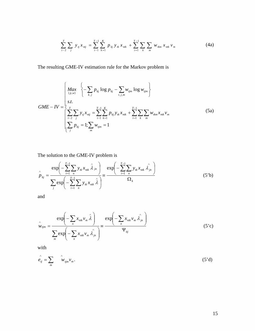
The resulting GME-IV estimation rule for the Markov problem is
⎪⎪⎪⎪
⎩
⎪⎪⎪⎪
⎨
⎧
==
+=
⎭⎬⎫
⎩⎨⎧
−−
=−
∑∑
∑∑ ∑∑ ∑∑∑
∑ ∑
−
−
− =
−
=
mtjm
jkj
m
T
t j
T
t
K
k
T
t k mntktkmntktkkjntjtj
jk mjttjmtjmkjkjwp
wp
vxwxypxy
ts
wwppMax
IVGME
1;1
..
loglog
2
1
1 1
1
1
, ,,},{
(5a)
The solution to the GME-IV problem is
k
T
t njnntktk
j
T
t nntktk
T
t njnntktk
kj
xy
xy
xyp
Ω
⎟⎠
⎞⎜⎝
⎛−
≡⎟⎠
⎞⎜⎝
⎛−
⎟⎠
⎞⎜⎝
⎛−
=∑∑
∑ ∑∑
∑∑−
=
∧
−
=
∧
−
=
∧
∧
1
11
1
1
1exp
exp
exp λ
λ
λ (5’b)
and
itj
njnmntk
m njnmntk
nmntk
tjm
vx
vx
vxw
Ψ
⎟⎟⎠
⎞⎜⎜⎝
⎛−
≡
⎟⎟⎠
⎞⎜⎜⎝
⎛−
⎟⎟⎠
⎞⎜⎜⎝
⎛−
=∑
∑ ∑
∑∧
∧
∧
∧λ
λ
λ exp
exp
exp (5’c)
with
.mm
tjmtj vwe ∑∧∧
= (5’d)
16
Maximizing equation 5 and solving forλ , yields the estimated∧
λ , which in turn yield the
optimal probabilities ∧
kjp and ∧
tjmw via equations (5’c) and (5’d). The GME and the
GME-IV optimization problem were programmed and solved using GAMS software. 8
ii. Diagnostics and Model Reliability
a) Sensitivity Analysis
The incremental or marginal effect of a change in bank-specific ( )( ntkz or macroeconomic
variables ( )tls on the transition probabilities ( )kjp can be derived from equation (5’b). The
marginal effect of each bank-specific covariate and macroeconomic variable on the
estimated transition probabilities is derived by differentiating equation (5’b) with respect
to ntkx :
⎥⎦
⎤⎢⎣
⎡−=
∂∂
∑j
jnkjjntkkjntk
kj pypxp
λλ (6a)
and evaluating at the means, or at any other value of interest, to capture the ‘dynamic’
effects of the market on the transition probabilities. These are used to inform the impact
on the stress test scenarios on the probability that a bank transitions to failure from each
of the other states as a result of a shock to the macroeconomic environment.
b) Goodness of Fit
The amount of information captured by the GCE-IV model can be measured using a
normalized entropy measure )~(PS defined in equation (6b).
∑∑∑∑
−
−≡
k j
okj
okj
k jkjkj
pp
ppPS ~ln~
~ln~
)~( (6b)
8 See Brook et. Al, (1992) for a further description of this algebraic modelling package.
17
with the kjp~ representing estimated transition probabilities under the GCE-IV estimation
rule and the oklp~ are the prior probabilities. )~(PS is bounded between 0 and 1, with 1
reflecting complete ignorance of the estimates and 0 reflecting perfect knowledge
(Golan, Judge, and Perloff, 1996b). In that way, )~(PS captures the amount of
information in the data relative to the initial knowledge reflected in the priors (Soofi,
1996). The normalized entropy measure, )~(PS can also be used to derive a pseudo- 2R
measure, a measure of in-sample goodness-of-fit, based on the normalized entropy S
(McFadden, 1974):
);~(12 PSRPseudo −≡ (6d)
c) Entropy Ratio
In addition, a likelihood ratio test of model fit can be constructed which is analogous to
that developed under the maximum likelihood (ML) procedure. That is, let ΩI be the
value of the optimal GCE objective function where the parameters of interest is
equivalent to minimizing (5a) subject to no constraints. Let ϖI be the constrained GCE-
IV model, constrained such that 0≠≠ λβ . Then, the Entropy Ratio (ER) static is defined
in equation (6c).
ER = ωII −Ω2 . (6c)
Under the null hypothesis, ER converges in distribution to .2)1( −Kχ Hence the ER static
can be used to evaluate the usefulness of the overall model.
18
Empirical Results
a) Evaluation of Unconditional and Conditional Transition Probability Matrices The prior probabilities are derived from the quarterly transition frequencies over the first
three years of the sample. They are computed as the mean of the percentage of banks in
state i in time t that fall in state j in time 1+t , .12.....,2,1,9,....,2,1, == tandji
These probabilities are estimated based on the mean behaviour of all banks within each
state in time t. Therefore this configuration makes the framework suited for identifying
systemic fragility which is a critical importance to supervisors. The prior probability
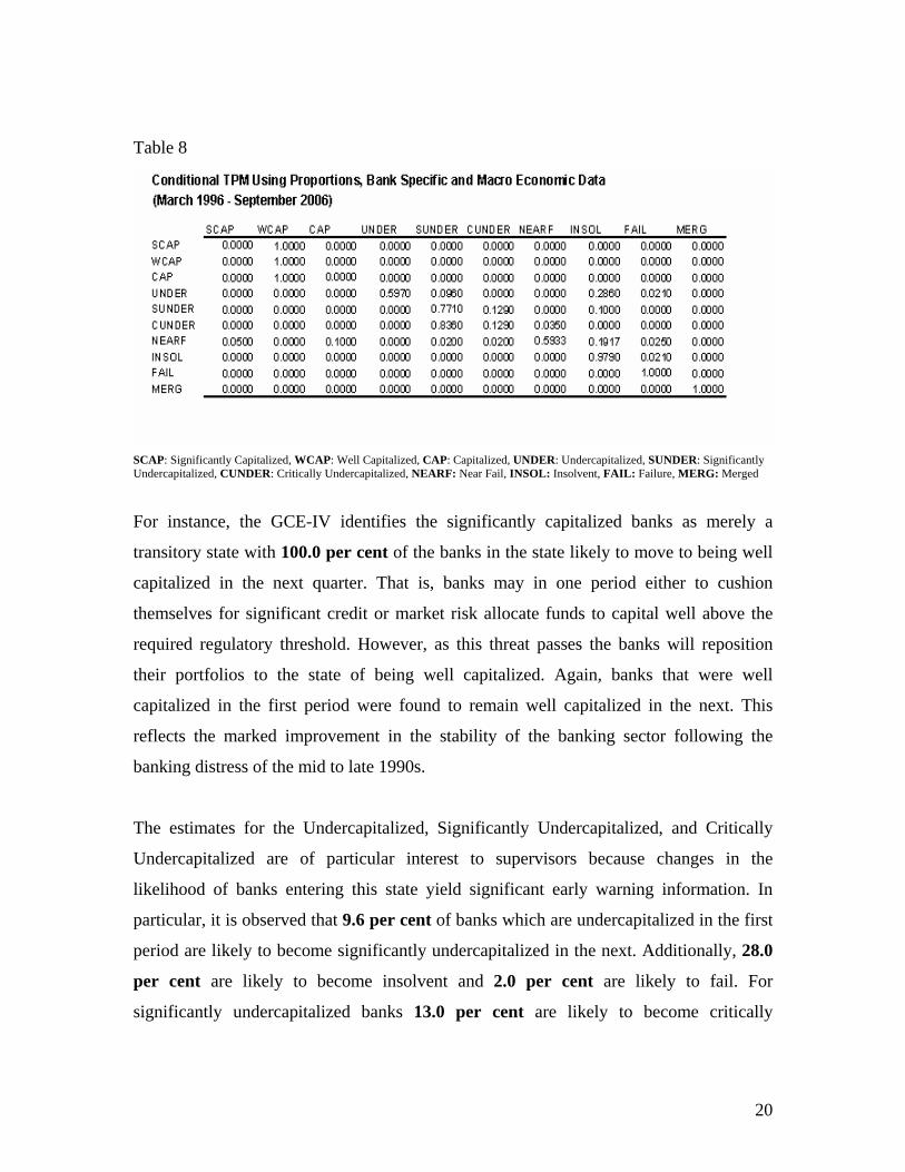
For instance, the GCE-IV identifies the significantly capitalized banks as merely a
transitory state with 100.0 per cent of the banks in the state likely to move to being well
capitalized in the next quarter. That is, banks may in one period either to cushion
themselves for significant credit or market risk allocate funds to capital well above the
required regulatory threshold. However, as this threat passes the banks will reposition
their portfolios to the state of being well capitalized. Again, banks that were well
capitalized in the first period were found to remain well capitalized in the next. This
reflects the marked improvement in the stability of the banking sector following the
banking distress of the mid to late 1990s.
The estimates for the Undercapitalized, Significantly Undercapitalized, and Critically
Undercapitalized are of particular interest to supervisors because changes in the
likelihood of banks entering this state yield significant early warning information. In
particular, it is observed that 9.6 per cent of banks which are undercapitalized in the first
period are likely to become significantly undercapitalized in the next. Additionally, 28.0
per cent are likely to become insolvent and 2.0 per cent are likely to fail. For
significantly undercapitalized banks 13.0 per cent are likely to become critically
21
undercapitalized and 10.0 per cent are likely to become insolvent. Finally, for Critically
Undercapitalized banks, 3.0 per cent are likely to become near failed institutions.
Interestingly, for near failed institutions it is estimated that 10.0 per cent are likely to
become capitalized in the next period and 5.0 per cent significantly capitalized in the
next period. This implies that banks can reposition their portfolios after a significant
shock to their capital position so as to rebound over the next period. This observation by
itself suggests that models which classify the transition process as binary are
underspecified. Along the main diagonal it is observed that banks increased the
likelihood of remaining well capitalized and significantly undercapitalized by 5.0 and
17.1 percentage points, respectively.
b) Sensitivity Analysis
Figures 1-3 report the marginal effects that selected bank-specific covariates and
macroeconomic variables would have on the estimated transition probability estimates.
The marginal effects show the direct effect of an increase in the bank-specific factor or
macroeconomic variables on each of the transition probabilities.
Incremental Effect of a Change in the Treasury Bill Rate (6-months)
The probability of a bank transitioning from being (WCAP) to being insolvent (INSOL)
increased by 0.004 for a 100.0 bps increase in the Treasury Bill rate. Again, there was a
0.001 increase in probability of a bank transitioning from being significantly capitalized
(SCAP) to significantly undercapitalized (SUNDER) for a 100.0 bps increase in the
Treasury Bill rate. On the other hand, the same marginal increase in the rate reduced the
probability of banks transitioning from undercapitalized (UNDER) to well-capitalized
(WCAP) by 0.018. These results suggest that, at least in the short run, positive interest
rate shocks have a measurable destabilizing impact on the financial health of the
commercial banking sector in Jamaica. This is likely due to the impact that an
instantaneous shock to interest rates would have on the re-pricing and maturity profiles of
banks before they had a chance to reposition their portfolios.
22
Figure 1. Incremental Effect of a Change in Treasury-bill Rate (6-months)
Incremental Effect of a Change in Net Interest Income (NII)
The probability of the representative bank transitioning from being well-capitalized
(WCAP) to insolvent (INSOL) decreases by 0.034 for a percentage point increase in net
interest income. Similarly, the probability of the representative bank transitioning from
well-capitalized (WCAP) to undercapitalized in the next quarter decreases by 0.038 for a
unit/percentage point increase in net interest income.
Figure 2.
Incremental Effect of a Change in Net Interest Income (NII)
INSO
L
CU
ND
ER
SU
ND
ER
UN
DE
R
CA
P
WC
AP
SCAP
NFA
IL
FAIL
SUNDERUNDER
CAPWCAP
SCAP
-0.2700
-0.2200
-0.1700
-0.1200
-0.0700
-0.0200
0.0300
0.0800
0.1300
0.1800
Cha
nge
TO
FROM
INSO
L
CU
ND
ER
SU
ND
ER
UN
DER
CAP
WC
AP
SCAP
NFA
IL
FAIL
SUNDER
UNDERCAP
WCAPSCAP
-0.1800
-0.1600
-0.1400
-0.1200
-0.1000
-0.0800
-0.0600
-0.0400
-0.0200
0.0000
Cha
nge
T0
FROM
-63.0%
-66.0%
-16.9%
23
These results are quite intuitive as, apriori, one would expect that increases in net interest
income of the bank would reduce the likelihood of transitioning from a higher state (e.g.
Capitalized) to a lower state (e.g. Insolvent).
Incremental Effect of a Change in the GDP Growth Rate
Positive shocks to GDP generally have a negative impact on the likelihood of
transitioning from higher state to a lower state. For example, a one per cent increase in
quarter over quarter annual GDP growth rate reduced the likelihood of transitioning from
being well capitalized (WCAP) to undercapitalized (UNDER) by 0.02.
Figure 3
Incremental Effect of a Change in the GDP Growth Rate
INS
OL
CU
ND
ER
SU
ND
ER
UN
DE
R
CAP
WC
AP
SCAP
NFA
IL
FAIL
SUNDERUNDER
CAPWCAP
SCAP
-0.200
-0.100
0.000
0.100
0.200
0.300
0.400
0.500
Cha
nge
TO
FROM
24
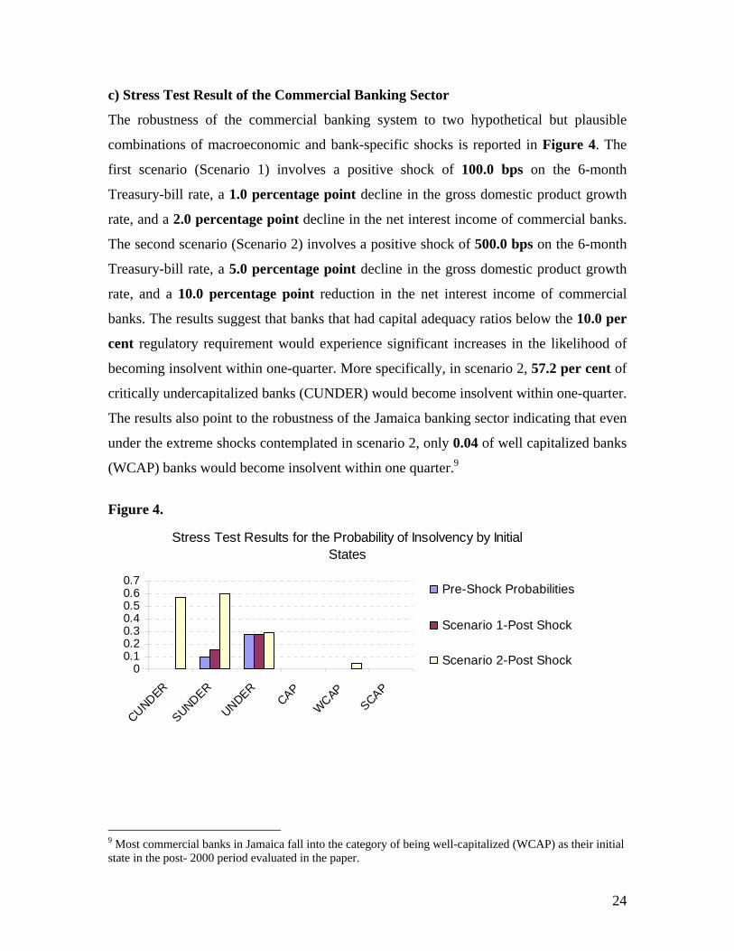
c) Stress Test Result of the Commercial Banking Sector
The robustness of the commercial banking system to two hypothetical but plausible
combinations of macroeconomic and bank-specific shocks is reported in Figure 4. The
first scenario (Scenario 1) involves a positive shock of 100.0 bps on the 6-month
Treasury-bill rate, a 1.0 percentage point decline in the gross domestic product growth
rate, and a 2.0 percentage point decline in the net interest income of commercial banks.
The second scenario (Scenario 2) involves a positive shock of 500.0 bps on the 6-month
Treasury-bill rate, a 5.0 percentage point decline in the gross domestic product growth
rate, and a 10.0 percentage point reduction in the net interest income of commercial
banks. The results suggest that banks that had capital adequacy ratios below the 10.0 per
cent regulatory requirement would experience significant increases in the likelihood of
becoming insolvent within one-quarter. More specifically, in scenario 2, 57.2 per cent of
critically undercapitalized banks (CUNDER) would become insolvent within one-quarter.
The results also point to the robustness of the Jamaica banking sector indicating that even
under the extreme shocks contemplated in scenario 2, only 0.04 of well capitalized banks
(WCAP) banks would become insolvent within one quarter.9
Figure 4.
Stress Test Results for the Probability of Insolvency by Initial States
00.10.20.30.40.50.60.7
CUNDER
SUNDER
UNDERCAP
WCAPSCAP
Pre-Shock Probabilities
Scenario 1-Post Shock
Scenario 2-Post Shock
9 Most commercial banks in Jamaica fall into the category of being well-capitalized (WCAP) as their initial state in the post- 2000 period evaluated in the paper.
25
Conclusions Recent turmoil in the capital markets has highlighted the need for systematic stress
testing of the banking sector. Less is known, however, about stress testing the portfolios
of banks to evaluate the impact that macroeconomic and bank-specific shocks have on
the susceptibility of banks to market and credit risks. The paper highlights the fact that
underlying macroeconomic volatility is a key aspect of the assessment of the fragility of
the banking sector and models which omit these factors are underspecified. Specifically,
sensitivity analysis conducted in the paper confirms that the Jamaican commercial
banking sector is bolstered by improvements in the growth of gross domestic product
(GDP), increases in the net interest income (NII) and hampered by positive unanticipated
shocks to interest rates. Moreover, stress-test analysis of commercials banks in the post
2000 period suggests that they are adequately capitalized to absorb significant adverse
combinations of macroeconomic shocks on both their balance sheets and income
statements.
26
References
Brooke, A., D. Kendrick and A. Meeraus, 1992, GAMS User’s guide; release 2.25. San Francisco; The Scientific Press. Caprio, Gerard, and Daniela Klingebiel, 1996, "Bank Insolvency: Bad Luck, Bad Policy, or Bad Banking?" Annual World Bank Conference on Development Economics 1996. Washington, D.C.: World Bank. Gavin, Michael, and Ricardo Hausman, 1996, “The Roots of Banking Crises: the Macroeconomic Context”, in Hausman and Rojas-Suarez (Eds.), Volatile Capital Flows: Taming their Impact on Latin America, Washington, Inter-American Development Bank. Glennon, D. and A. Golan, 2003, “A Markov Model of Bank Failure Estimated Using an Information-Theoretic Approach” The American University Press Golan, Amos; G. Judge; and J. M. Perloff, 1997, Estimation and inference with censored and ordered multinomial data, Journal of Econometrics, 1997 Honohan, Patrick, 1997, "Banking System Failures in Developing and Transition Economies: Diagnosis and Prediction", Bank for International Settlements Working Paper No. 39. International Monetary Fund, 2003, Research Bulletin, Washington, DC. Jaynes, E.T., 1957a, Information theory and statistical mechanics, Physics Review 106, 620-630 Kaminsky, Graciela L., and Carmen M. Reinhart, 1998, “On Crises, Contagion, and Confusion,” forthcoming in Journal of International Economics. Lindgren, Carl-Johan, Gillian Garcia, and Matthew Saal, 1996, Bank Soundness and Macroeconomic Policy (Washington: International Monetary Fund). MacRae C. Elizabeth, 1977. “Estimation of Time-Varying Markov Processes with Aggregate Data,” Econometrica, Vol. 45, No.1. (January 1977) pp. 183-198. McFadden, D. 1974, “Conditional logit analysis of qualitative choice behaviour”, in Zarembka, P. (ed. by), Frontiers in econometrics, Academic Press, New York, pp. 105-142.
27
Sachs, J., A. Tornell and A. Velasco, “The Collapse of the Mexican Peso: What Have We Learned?” Economic Policy 22, 1996a, 13-56. Soofi, E. S. (1996) "Information Theory and Bayesian Statistics", in Bayesian Analysis of Statistics and Econometrics, in D. Berry, K. Chaloner, and J. Geweke (eds.), 179-189, New York: Wiley. Zepeda, L., 1995b, Technical change and the structure of production: A non–stationary Markov analysis, European Review of Agricultural Economics, 41–60.


![JAMAICA - Food and Agriculture Organizationextwprlegs1.fao.org/docs/pdf/jam165343.pdf · JAMAICA No. 1 -2016 I assent, [L.S.] f?ryd. Governor-General. AN ACT to Repeal the Jamaica](https://static.documents.pub/doc/80x56/5f59904ed4257a7c0d649234/jamaica-food-and-agriculture-org-jamaica-no-1-2016-i-assent-ls-fryd-governor-general.jpg)


