AN ECONOMIC ANALYSIS OF GRID-CONNECTED RESIDENTIAL SOLAR PHOTOVOLTAIC POWER SYSTEMS Paul R. Carpenter and Gerald A. Taylor M.I.T. ENERGY LABORATORY REPORT - MIT-EL 78-007 May 1978 Revised December 1978 PREPARED FOR THE UNITED STATES DEPARTMENT OF ENERGY Under Contract No. EX-76-A-01-2295 Task Order 37
Transcript
AN ECONOMIC ANALYSIS OF GRID-CONNECTED RESIDENTIALSOLAR PHOTOVOLTAIC POWER SYSTEMS
Paul R. Carpenter and Gerald A. Taylor
M.I.T. ENERGY LABORATORY REPORT - MIT-EL 78-007
May 1978
Revised December 1978
PREPARED FOR THE UNITED STATES
DEPARTMENT OF ENERGY
Under Contract No. EX-76-A-01-2295Task Order 37
THE ECONOMIC AND POLICY IMPLICATIONSOF GRID-CONNECTED RESIDENTIAL SOLAR
PHOTOVOLTAIC POWER SYSTEMS
BY
Paul R. Carpenter
Gerald A. Taylor
ABSTRACT
(Revised)
The question of the utility grid-connected residential market for
photovoltaics is examined from a user-ownership perspective. The priceis calculated at which the user would be economically indifferent between
having a photovoltaic system and not having a system. To accomplishthis, a uniform methodology is defined to determine the value to theuser-owner of weather-dependent electric generation technologies. Twomodels are implemented for three regions of the United States, the firstof which is a previously developed simulation of a photovoltaicresidence. The second is an economic valuation model which is requiredto translate the ouputs from the simulation into breakeven array prices.Special care is taken to specify the input assumptions used in the
models. The accompanying analysis includes a method for analyzing theyear-to-year variation in hourly solar radiation data and a discussion ofthe appropriate discount rate to apply to homeowner investments inphotovoltaic systems.
The results of this study indicate that for the regions
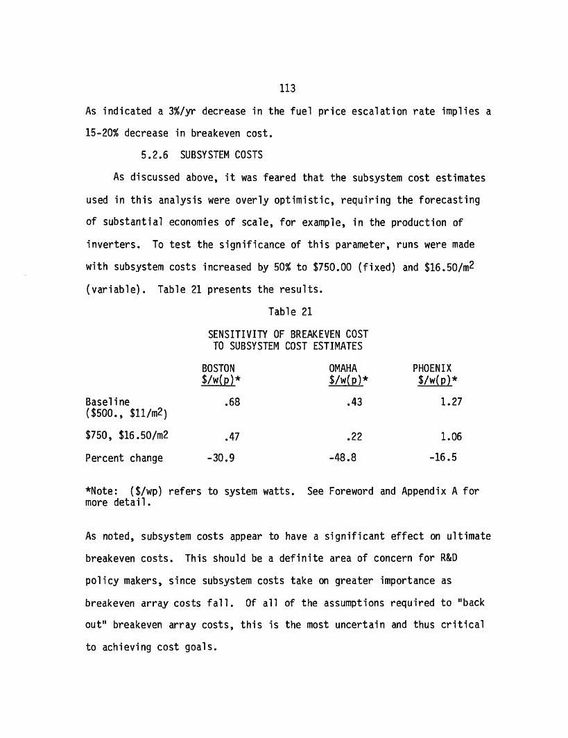
characterized by Boston, Omaha, and Phoenix, under the assumptions noted,photovoltaic module breakeven costs for the residential application arein the range of $.68, $.43 and $1.27 per peak system watt respectively
(.42, .24, .89 per peak module watt).
3
FOREWORD TO REVISED VERSIONDecember 1978
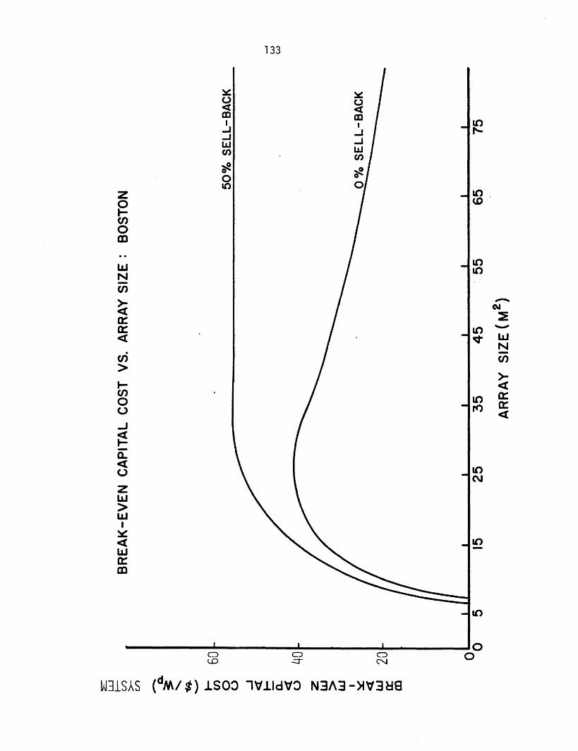
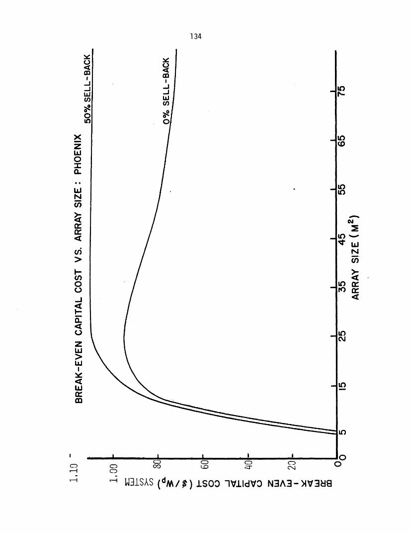
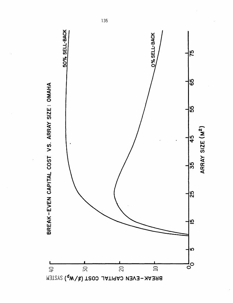
Appendix A to this volume presents revised values for breakeven
capital costs for photovoltaic modules in residential applications. Inthe main body of the report, specifically in Section V, the measure forBECC, dollars/watt (peak), as reported in this paper is in delivered,system or effective peak watts (module). The use of dollars/watt (peak)is somewhat ambiguous in the literature; it is necessary to point outthat this measure is not dollars/watt (peak) of module output. Themethodology used in this study consistently focuses upon deliveredenergy. The system NPV figure is the value of the energy delivered bythe particular system under consideration - the valuation procedure perse is not sensitive to the efficiency of the system which delivers theenergy.
Conversion from a dollars/watt (peak) system is a straightforwardalgebraic process. The dollars/m2 figure is the same in bothsituations; the question relates to the number of watts of deliveredenergy at either the system or the module; and this question is merelywhich n(efficiency), system or module, to use in the conversion:
Dollars/watt (peak) system= Dollars/m2
nsystem x 1000w/m2
Dooars/watt (peak) module = Dollars/m2
nmodule x 1000w/m2
Since n(system) is used multiplication of the values listed in thisreport by n(system)/n(module) will yield a dollar value for module peakwatts.
The results presented in Aopendix A incorporate the results ofresearch in cell efficiency, increased information on balance of systemscosts and results of discussion and comment concerning the May 1978version of this paper. For this reason these values should be used torepresent current best estimates of breakeven capital costs forphotovoltaic modules in residential applications.
4
TABLE OF CONTENTS
Page
Abstract 2
Foreword to Revised Version 3
Table of Contents 4
Table of Tables 7
Table of Figures 9
Acknowledgment 10
I. Solar Photovoltaics as an Electric Power Source 11
1.1 Introduction 11
1.2 History of the Federal Photovoltaics Program 13
1.3 Photovoltaic Market Segments and TheirRelationship to the Federal Plan 17
1.4 Scope of This Study 22
1.5 Footnotes 24
II. A Uniform Economic Valuation Methodology 27
2.1 Introduction 27
2.2 Economic Valuation of Photovoltaics 29
2.3 Unique Features of Photovoltaics WhichAffect Economic Valuation 30
III. Simulation Model Description and Input Assumptions
3.1 Regional Definition
3.2 Valuation Model
3.3 Model Inputs
3.3.1 System Configuration
3.3.2 Insolation Data
3.3.3 Appliance Loads and BehavioralAssumptions
3.3.4 Rate Schedules
3.4 Footnotes
IV. Economic Model Inputs and Sensitivity
Analysis Assumptions
4.1 Fuel Price Escalation and Cell
Degradation Rate
4.2 Discount Rate
4.3 Subsystem Costs
4.4 Footnotes
V. Results and Interpretation
5.1 Basic Results by Array Size
5.2 Sensitivity Analysis
5.2.1 Choice of Year
5.2.2 Discount Rate
5.2.3 Degradation Rate
5.2.4 Cell Efficiency
Page
43
43
45
50
50
52
54
59
69
73
73
75
86
90
94
94
107
107
110
110
111
6
TABLE OF CONTENTS (continued)
Page
V. (continued)
5.2.5 Fuel Price Escalation 111
5.2.6 Subsystem Costs 113
5.3 Comparison of Results to Utility Studies 114
5.4 Footnotes 117
VI. Policy Implications and Conclusions 119
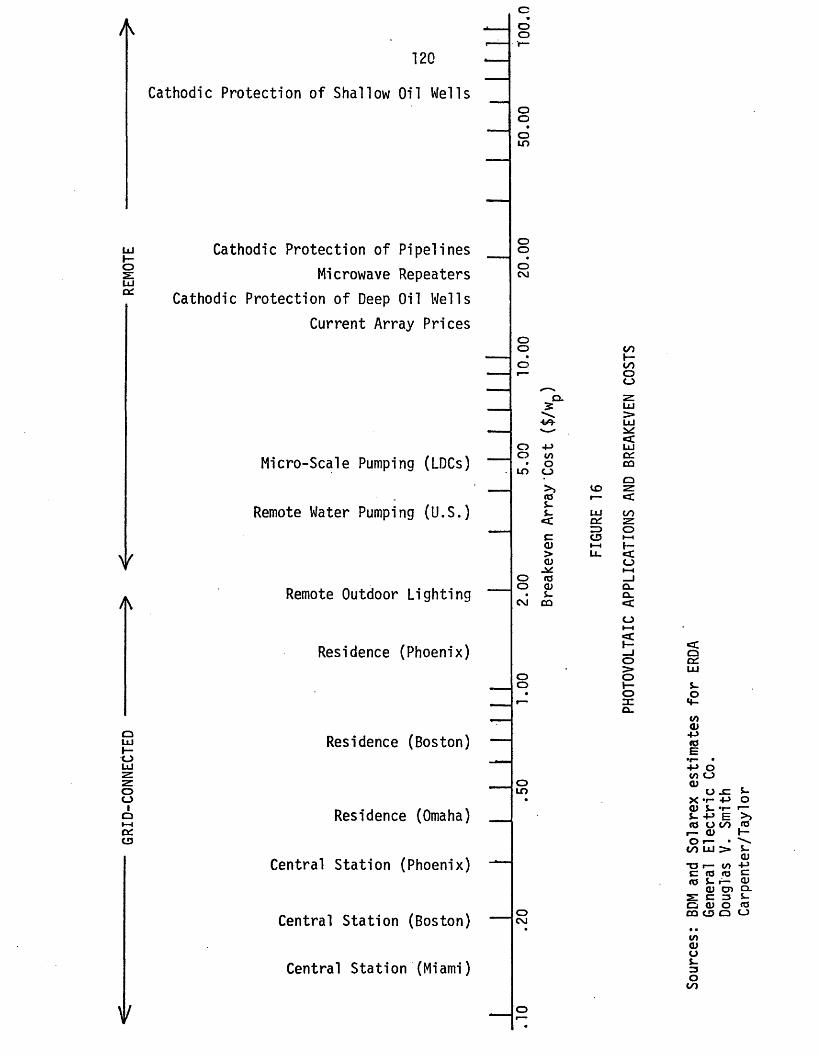
6.1 New Information 119
6.2 Implications for the Long-Term Markets 119
6.3 Implications for Systems Tests andApplications (ST&A) Policy 122
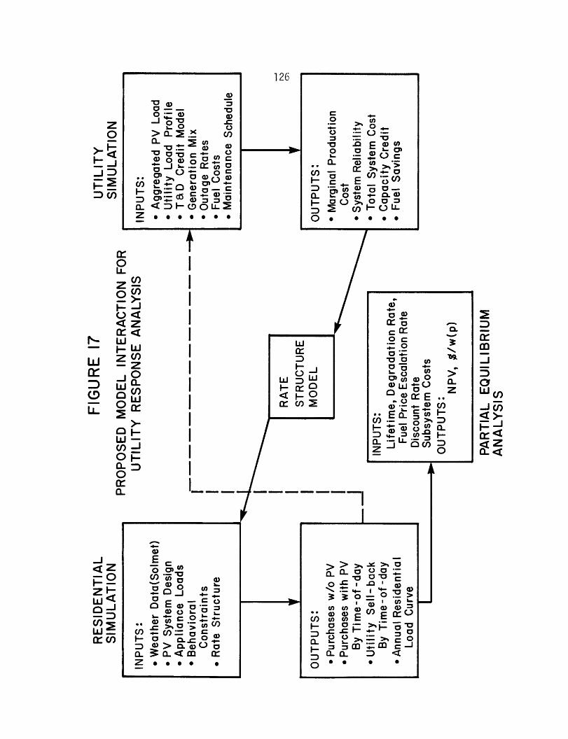
6.4 Utility Response and Interactive Models:Further Research 123
6.5 Conclusion 125
6.6 Footnotes 129
VII. Appendices 131
VIII. Bibliography 157
TABLE OF TABLES
Table Page
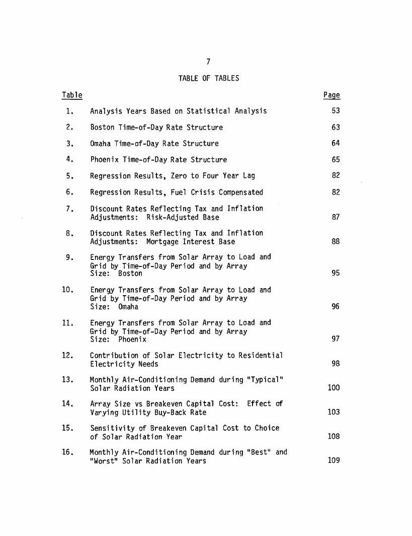
1. Analysis Years Based on Statistical Analysis 53
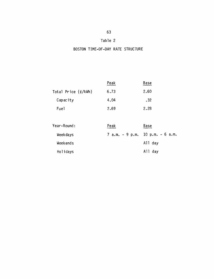
2. Boston Time-of-Day Rate Structure 63
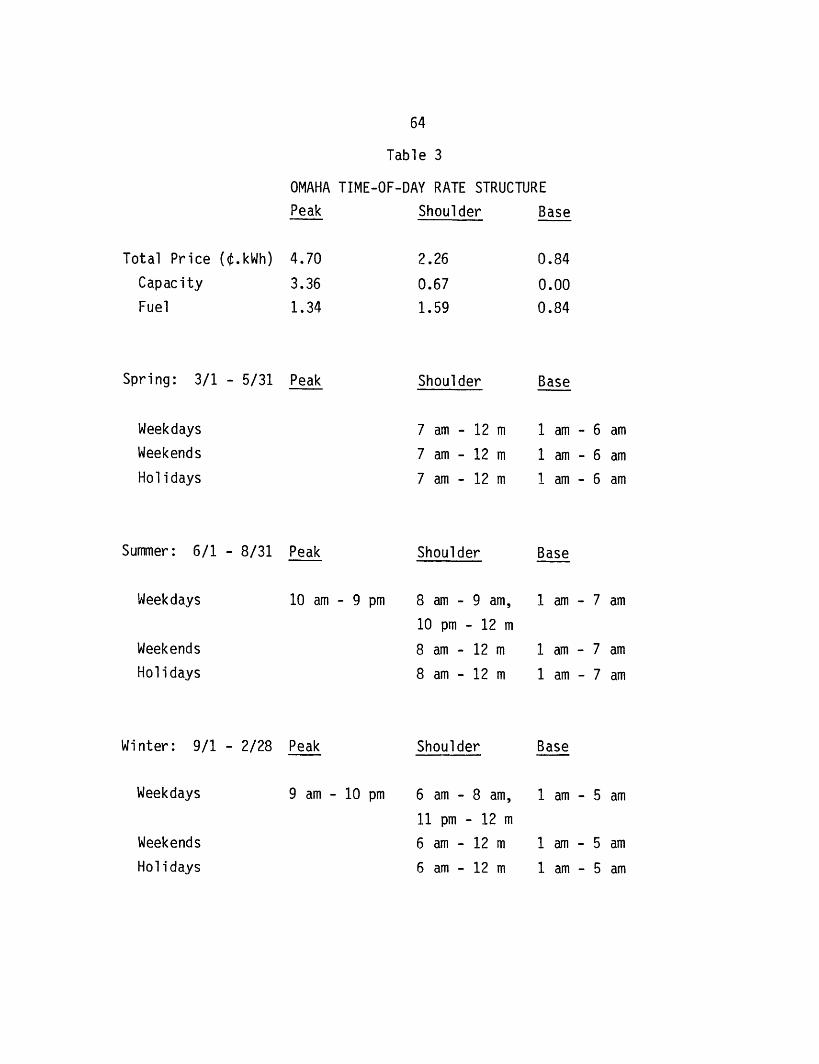
3. Omaha Time-of-Day Rate Structure 64
4. Phoenix Time-of-Day Rate Structure 65
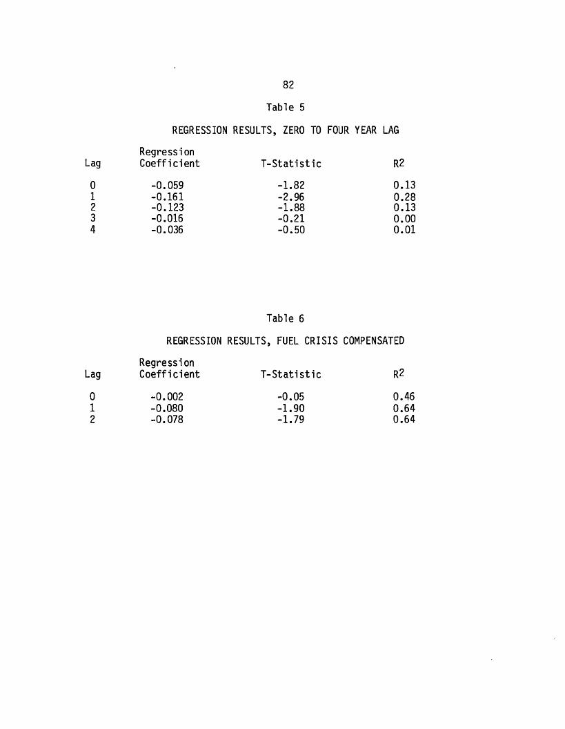
5. Regression Results, Zero to Four Year Lag 82
6. Regression Results, Fuel Crisis Compensated 82
7. Discount Rates Reflecting Tax and InflationAdjustments: Risk-Adjusted Base 87
8. Discount Rates Reflecting Tax and InflationAdjustments: Mortgage Interest Base 88
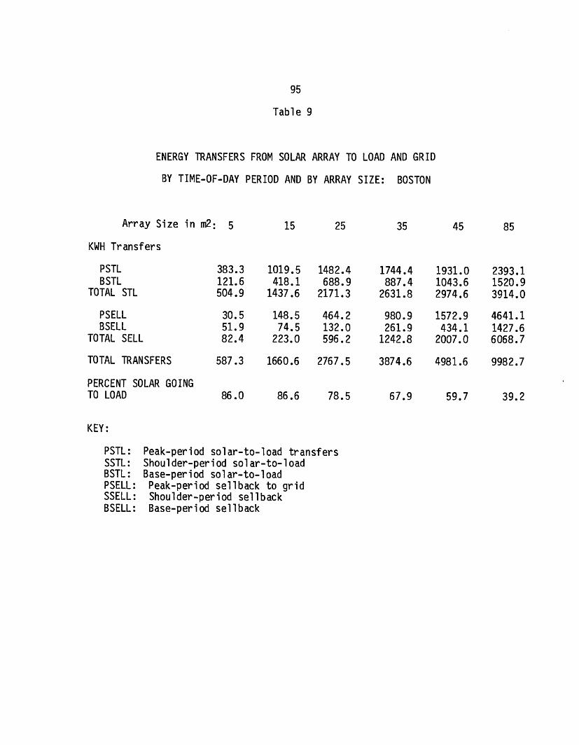
9. Energy Transfers from Solar Array to Load andGrid by Time-of-Day Period and by ArraySize: Boston 95
10. Energy Transfers from Solar Array to Load and
Grid by Time-of-Day Period and by ArraySize: Omaha 96
11. Energy Transfers from Solar Array to Load andGrid by Time-of-Day Period and by ArraySize: Phoenix 97
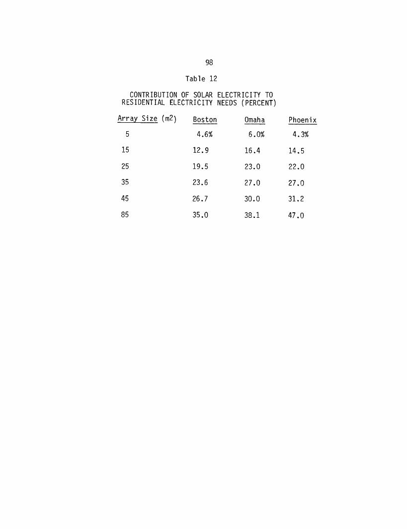
12. Contribution of Solar Electricity to Residential
Electricity Needs 98
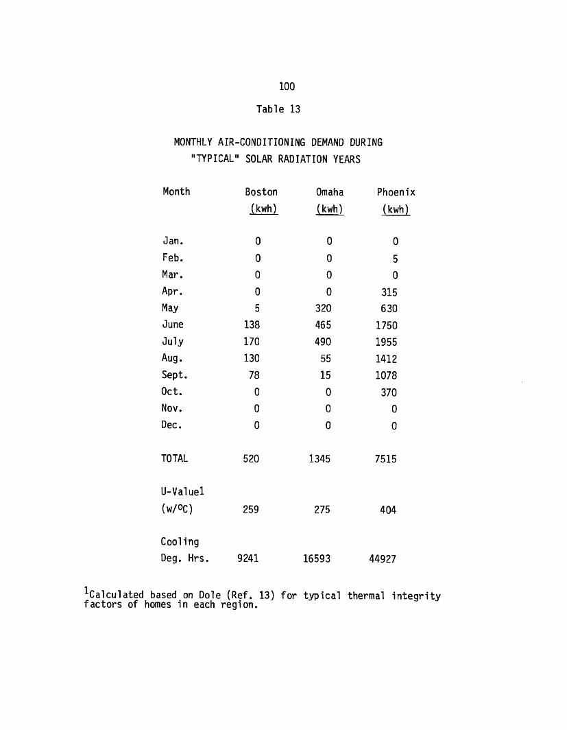
13. Monthly Air-Conditioning Demand during "Typical"Solar Radiation Years 100
14. Array Size vs Breakeven Capital Cost: Effect of
Varying Utility Buy-Back Rate 103
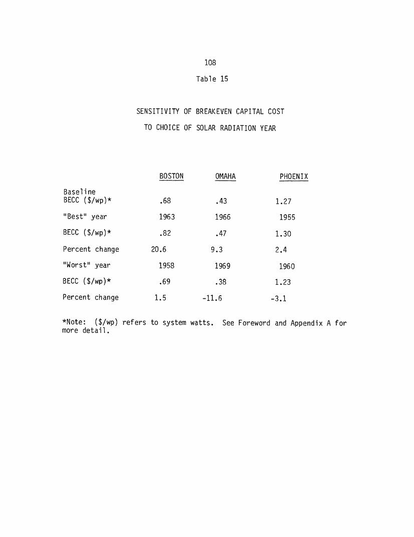
15. Sensitivity of Breakeven Capital Cost to Choiceof Solar Radiation Year 108
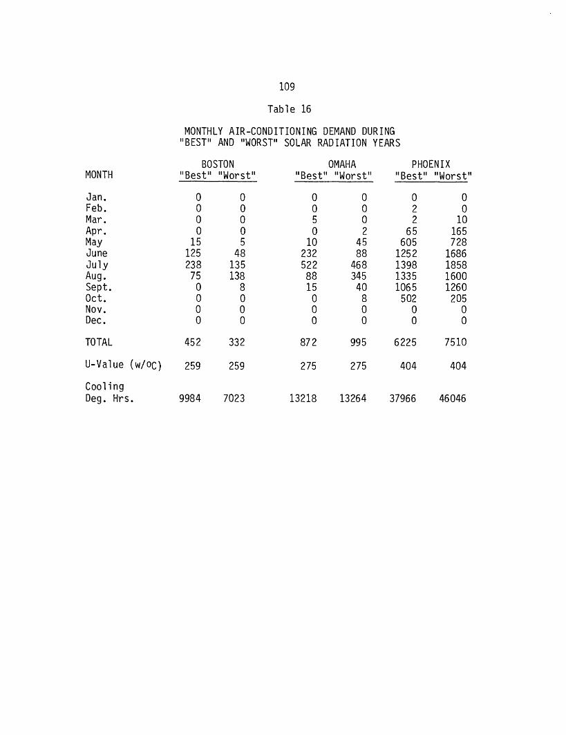
16. Monthly Air-Conditioning Demand during "Best" and
"Worst" Solar Radiation Years 109
8
TABLE OF TABLES (continued)
Table Page
17. Effect of Varied Discount Rate on Breakeven Cost 110
18. Sensitivity of Breakeven Cost to Altered DegradationRates 111
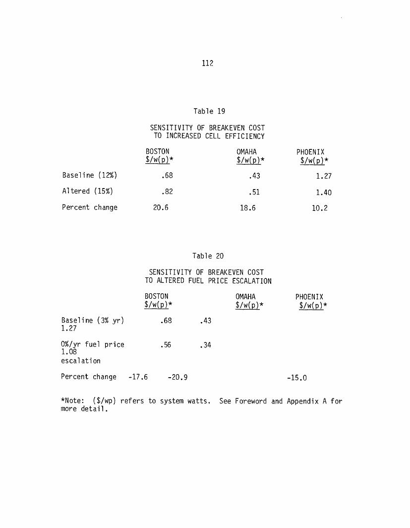
19. Sensitivity of Breakeven Cost to IncreasedCell Efficiency 112
20. Sensitivity of Breakeven Cost to AlteredFuel Price Escalation Rate 112
21. Sensitivity of Breakeven Cost to SubsystemCost Estimates 113
9
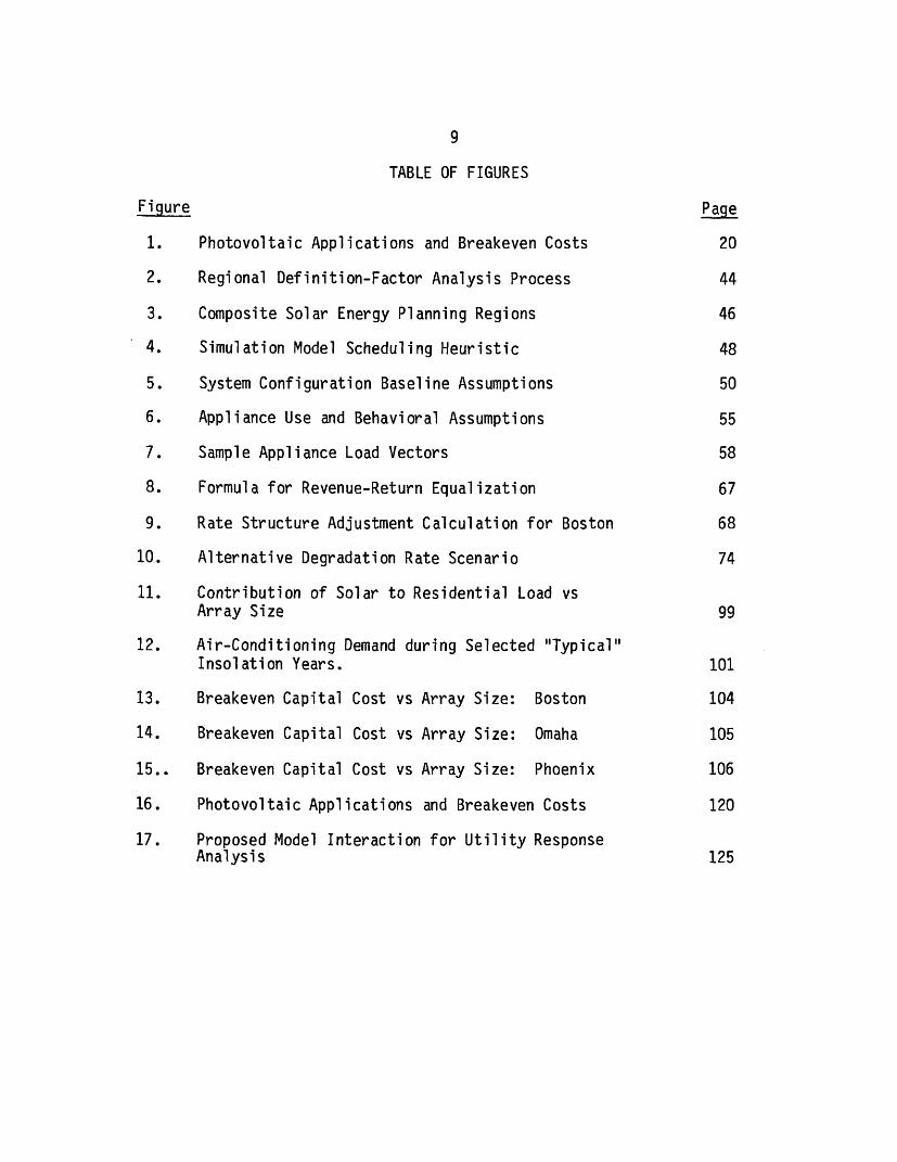
TABLE OF FIGURES
Figure Page
1. Photovoltaic Applications and Breakeven Costs 20
2. Regional Definition-Factor Analysis Process 44
3. Composite Solar Energy Planning Regions 46
4. Simulation Model Scheduling Heuristic 48
5. System Configuration Baseline Assumptions 50
6. Appliance Use and Behavioral Assumptions 55
7. Sample Appliance Load Vectors 58
8. Formula for Revenue-Return Equalization 67
9. Rate Structure Adjustment Calculation for Boston 68
10. Alternative Degradation Rate Scenario 74
11. Contribution of Solar to Residential Load vsArray Size 99
12. Air-Conditioning Demand during Selected "Typical"Insolation Years. 101
13. Breakeven Capital Cost vs Array Size: Boston 104
14. Breakeven Capital Cost vs Array Size: Omaha 105
15.. Breakeven Capital Cost vs Array Size: Phoenix 106
16. Photovoltaic Applications and Breakeven Costs 120
17. Proposed Model Interaction for Utility ResponseAnalysis 125
10
ACKNOWLEDGEMENT
While many individuals have greatly contributed to the development
of this study, several deserve special recognition. The authors would
especially like to thank Jesse Tatum of the MIT Energy Laboratory for his
many hours devoted to the development of the simulation model used to
generate the results herein. Others who made special contributions
include Ms. Susan Finger, Mr. Drew Bottaro, Dr. Lawrence H. Linden, and
Dr. Neil Goldman of the MIT Energy Laboratory Photovoltaics Project, and
Dr. Jeffrey L. Smith of the Jet Propulsion Laboratory LSA Project, and
Alice Sanderson, whose typing efforts were greatly appreciated. Finally
we wish to thank Professor Henry Jacoby, our Sloan School thesis adviser,
for his many helpful comments and criticisms and, above all, Dr. Richard
Tabors, manager of the MIT Energy Laboratory Photovoltaics Project, for
his unfailing support and assistance and his Vermont mountain retreat.
Paul Carpenter
Gerald Taylor
11
I. SOLAR PHOTOVOLTAICS AS AN ELECTRIC POWER SOURCE
1.1 INTRODUCTION
Among the emerging technologies which may provide solutions to
current energy problems, photovoltaic power is, perhaps, the most
unique. Without moving parts or intermediate thermal conversion, the
sun's radiation is converted directly into usable electric power.
Because of the peculiar properties of the semiconductor materials which
make up photovoltaic cells (often called "solar cells"), incident
sunlight creates an electrical potential which can be used to generate a
flow of electrons, or electric current. Individual cells, each creating
a small amount of electricity, can be linked to produce energy in amounts
suitable for myriad practical applications including central power
(utility) stations.
The characteristics of any technology naturally have a great deal of
impact upon its development and practical application. The nature of
photovoltaic cells is such that there appears to be great potential
advantage in their application. On the other hand, there are substantial
practical problems which mitigate the technology's positive aspects and
there appear to be some disadvantages as well that have not yet received
much attention. While, for instance, the modularity of PV cells and the
concomitant absence of significant economies of scale imply that energy
can be produced in small quantities without high costs per unit output,
the electricity produced is direct current which must be converted
12
to alternating current for most conventional uses by power-conditioning
equipment (inverters). Inverters do exhibit scale economies and thus the
advantages of modularity are offset by the need for power conditioning.
Another advantage of the PV technology is its lack of moving parts which
makes it ideal for remote or residential applications where generating
equipment must operate for long periods while unattended. But such
unattended applications require module designs which are both very safe
and durable and the expense of achieving such designs is significant.
Finally PV technology is frequently advocated as an ideal energy source
because of the absence of such negative externalities as pollution.
While it is true that PV devices produce energy without emitting
pollutants there are other problems associated with widespread use.
These problems include occupational and safety hazards during production
and maintenance of photovoltaic cells, and extremely heavy energy
consumption in the production of the semiconductor materials.1
The process of selecting development applications which economically
achieve a favorable balance of these positive and negative
characteristics is bound to be a difficult one requiring not only careful
analysis but also a well-directed and documented testing program. Given
a catalogue of the technology's characteristics a logical first step in
such a selection process might be to identify applications for further
study which exhibit positive aspects of photovoltaics while avoiding,
insofar as possible, negative aspects. Since there is so
13
much uncertainty surrounding photovoltaic development (as with any new
technology) both in terms of production and potential markets, another
criterion in the selection process might be an application's potential
for an orderly progression both in the acquisition of practical
experience with the technology and market and production growth. A final
factor to be considered, especially from a governmental policy
perspective, is an application's commercial potential, i.e. capability to
compete on its own in the marketplace. Other things being equal, the
more rapidly an application achieves market competitiveness, the better
for the taxpayer since governmental development or commercialization
subsidies should no longer be necessary for a competitive product.
Before turning to a discussion of the relationship between specific
photovoltaic applications or market segments and their
economic/commercial potential (and how one goes about analyzing that
potential), a short digression on the history of the Federal
Photovoltaics Program is in order. This history is important because it
has been perhaps the most aggressive of the technology development
programs at the Department of Energy since nuclear power, and its nature
has broad implications for the kinds of information required from the
economic analysis of photovoltaic applications.
1.2. HISTORY OF THE FEDERAL PHOTOVOLTAICS PROGRAM
Since its inception in the early 1970s, the Photovoltaics Program
within the Energy Research and Development Administration (now Department
14
of Energy) has focused its effort on driving the costs of photovoltaic
devices down. This approach is manifested in several program objectives,
actors, and concepts.
The specific objectives of the National Photovoltaic Conversion
Program were first articulated at the NSF/RANN Cherry Hill, New Jersey
Conference in the fall of 1973. Program goals were here for the first
time described in terms of array costs. "It is anticipated that
large-scale application of solar photovoltaic technology will become
economically viable by approximately 1980. This will be made possible by
the reduction of solar array cost to less than $0.50/watt (peak)." 2 ,3
At the time this number was not supported with economic analysis of
potential applications. It was later established by ERDA as its 1986
Photovoltaics Program goal.4 Given the state of knowledge of
photovoltaic technology and its applications at the time, the Cherry Hill
statement of program objectives was not unreasonable.* But much faith
has been placed in that number as a target for economic value,
independent of any particular applications environment or region.
Given the history of the photovoltaic conversion technology as a
satellite power system, it is not surprising that many of the actors in
the Photovoltaics Program were also actively involved in the space
*Since $0.50/watt(p) represented a good estimate of 5/kWh translated tophotovoltaic array terms.
15
program. The Jet Propulsion Laboratory through its Low Cost Silicon
Solar Array Project is one such organization that now has primary
responsibility for the development of a low-cost silicon technology.5
"The primary goal of the LSSA Project is to develop by 1986 the
technological and industrial capability to produce silicon solar
photovoltaic arrays at a rate of more than 500 peak MW per year, having
an efficiency of greater than 10 percent and a 20-year minimum lifetime,
at a market price of less than $500 per peak KW, ($0.50/watt(peak))."6
Thus, the JPL program is utilizing its experience in space program
management to generate technical and production advances (supply-side
phenomena) to meet the 1986 Cherry Hill/ERDA objective. The Aerospace
Corporation, another space program actor, has performed a set of "Mission
Analyses" of photovoltaic applications in residential, commercial and
central station applications which brought together first-order technical
performance and financial analyses. 7 In the majority of the research
and development effort to date the program has placed primary effort on
attainment of the goals, a legacy of the space program, and secondary
emphasis on the costs of accomplishing this research and development.
Given the program objectives and actors it is not hard to understand
the concept behind the commercialization of photovoltaics in the program,
a concept that has been characterized as a "market-pull" philosophy. The
essence of this concept is that government purchases of photovoltaic
cells, independent of their use in particular applications, is enough of
a stimulus to drive the photovoltaic industry down the experience curve
and thus meet the 1986 cost goals. This was articulated in the 1976
Photovoltaics Program plan:
16
a stimulus to drive the photovoltaic industry down the experience curve
and thus meet the 1986 cost goals. This was articulated in the 1976
Photovoltaics Program plan:
It is expected that ERDA purchases of approximately 600 KWe through
FY78, coupled with purchases by other federal agencies with ERDA'ssupport, will result in a factor of 4 reduction in the present cost
of silicon-based solar cells...A total government purchase ofapproximately 11 MW through FY 1983 is planned. Costs for silicon
solar cell arrays are expected to drop to $1000 per peak KW by1984.8
"Market-pull" is a concept that is rational given the objectives and
actors described above, especially in a situation where achieving cost
goals is the primary objective. At present, however, there appears to be
a greater realization that future strategies for the commercialization of
photovoltaics require that attention be focused on the marketplace,
particularly the marketplace in which electric utilities reside.
More recently, in the latest National Photovoltaic Program Plan,9
an even more aggressive eight-cycle, eight-year photovoltaic procurement
initiative has been proposed that would cost the government approximately
$380 million. The purpose of this new initiative is to accelerate by
several years the diffusion of photovoltaic devices into the
markeplace.l0 The "market-pull" concept has been institutionalized in
terms of the so-called PRDA (Program Research and Development
Announcement) which is the mechanism whereby the government solicits
proposals from private sector interests to be recipients of these
government-purchased modules for tests and applications purposes. This
17
new plan includes the same program goals as described above but they are
now time-phased as follows.11
Near-term
To achieve prices of $2 per peak watt (1975 dollars) at an
annual production rate of 20 peak megawatts in 1982.
· Mid-term
To achieve prices of $0.50 per peak watt, and an annual
production rate of 500 peak megawatts in 1986.
· Far-term
To achieve prices of $0.10 to $0.30 per peak watt in 1990, and
an annual production rate of 10-20 peak gigawatts in 2000.
1.3. PHOTOVOLTAIC MARKET SEGMENTS AND THEIR RELATIONSHIP TO THEFEDERAL PLAN
Several attempts have been made to attach particular applications to
the set of time/price horizons above. Before discussing the evidence
which has accumulated to date, let us briefly consider the variety of
potential photovoltaic markets and their characteristics.
While there are myriad potential uses for photovoltaics, most
applications seem to fall into three major categories: remote
applications, grid-competing (or load-center) applications, and
grid-connected applications.
Remote Applications
This set of applications is composed of small-scale stand-alone
systems that take advantage of the low maintenance and modularity
18
features of the technology. They include satellites, ocean buoys,
cathodic protection, micro-scale agricultural pumping and other
military-related applications. As can be seen, this set is made up of
applications which heretofore had no (or very expensive) alternative
energy sources. This fact means that these users are willing to pay a
very high price for photovoltaic power and thus all current production is
geared toward these uses. The remote market is not important with
respect to the world's energy problems and in relative terms the market
is very small.
Grid-Competing Applications
This set of applications includes those load centers which would
otherwise need to be connected to the utility grid. A typical
configuration would be a school or industrial plant with a large set of
photovoltaic arrays supplemented by backup power from a diesel generator
or other source. The category could also include a stand-alone house
with some form of solar heating and cooling and electrical and thermal
storage system for uninterrupted use. As one might guess, this set of
applications may also be somewhat limited in market size due to the
relatively low marginal cost of attaching oneself to the utility grid.
To operate independent of the grid would imply the payment of a "premium"
in the form of high capital costs in order to be totally independent.
Grid-Connected Applications
Since nearly all electricity generated in the United States is
produced by large electric utilities, if the objective of the
19
commercialization of photovoltaic technology is to replace some of this
conventional generation capacity, then the long-term market for
photovoltaics is the grid-connected market. This set includes
residences, schools, industrial and commercial establishments (in
dispersed mode) as well as central station photovoltaic applications.
There appear to be few technical problems associated with the interplay
between on-site photovoltaic power as it is fed back into the grid and
the use of electricity from the grid when the solar power is
insufficient.12
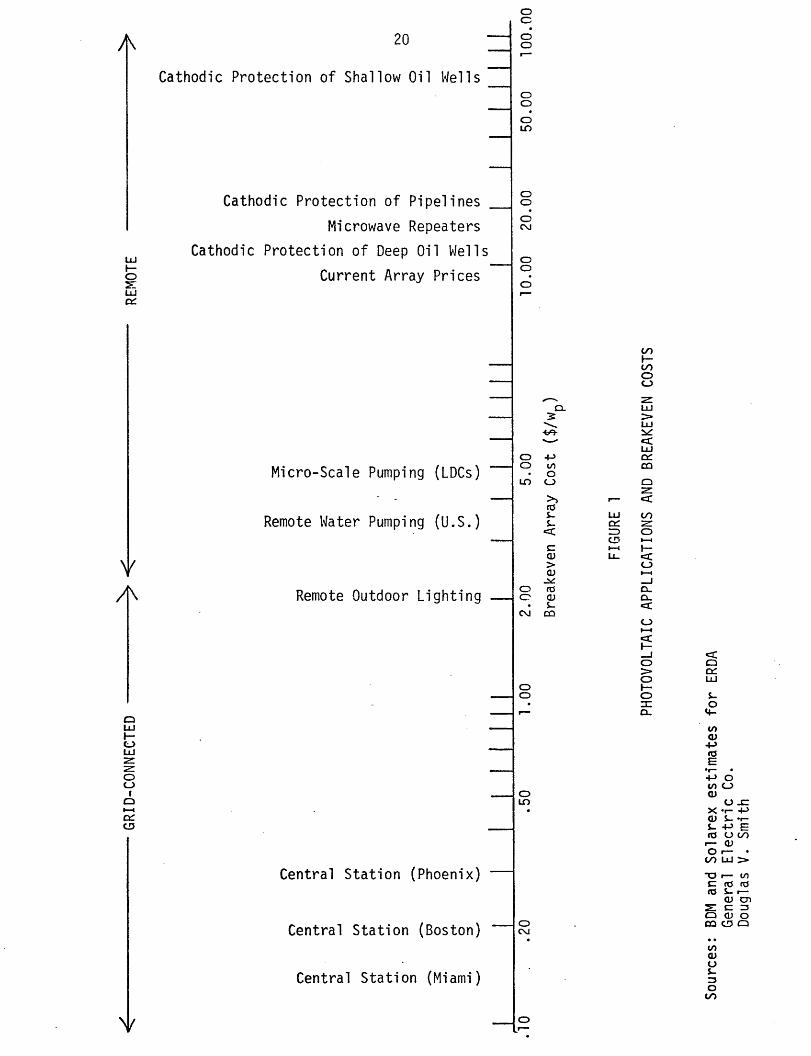
It was mentioned above that several attempts have been made to
attach various applications to the time/price framework of the National
Plan. Figure 1 represents a plot of the various applications which have
been studied and the "competitive" prices associated with those
applications. As can be seen, there are significant gaps in the
knowledge,1 3 particularly with respect to breakeven prices of
grid-connected applications, not to mention knowledge of the potential
quantities demanded at these prices. As yet, no adequate measure of
potential quantities demanded in the grid-connected market has been
developed. As will be suggested later, one way to approach this question
is to examine the effects of added penetration on utility system costs.
While this method does not estimate a future demand curve, it does offer
a means of defining demand potential. The best information available to
date on the effect of photovoltaics on the utility system has been
20
Cathodic Protection of Shallow Oil Wells
Cathodic Protection of Pipelines
Microwave Repeaters
Cathodic Protection of Deep Oil Wells
Current Array Prices
Micro-Scale Pumping (LDCs)
Remote Water Pumping (U.S.)
Remote Outdoor Lighting
Central Station (Phoenix) -
Central Station (Boston) -
Central Station (Miami)
0
u)
I"
U-)
O
30o
o 4-A
co
Ui
U"
* S.-
C
0'N
LU
I-zr-UL
/
C(
C)
L u>I-,:cscmz
CD
_
C)3..(,.0.
.-
LJ
LJ
zCu
-
cD
C)iY
04-(n
t,E4-' 0
cn ;a) U
L.) C
o)L V)0 SL r
X C
oVi)
/
21
provided by the work of General Electric14 and Westinghouse1 5 with
regard to the effect of central station photovoltaic plants on utility
reliability and thus, costs. This valuation of the central station
application was a reflection of the study authors' orientation as well as
the focus of the Federal Program several years ago. The results of the
central station studies show that photovoltaic power plants improve
utility system reliability and thus do not require 100% backup; however,
the breakeven prices calculated were low relative to the Program goals.
It should be noted that these studies considered the residential
application, but their analysis required utility ownership of the systems
and thus the framework in which their financial analysis was performed
failed to capture many of the potential advantages of residential,
user-owned systems which will be elaborated upon later. General
Electric, in its Requirements Assessment study, recognized this fact:
It is not possible to define the breakeven capital cost for a
user-owned PEPS (Photovoltaic Electric Power System) plant in thesame way as has been done for utility-owned plants. This is becausethe economic incentive to purchase and install such a plant lies inthe savings in purchased electricity costs accruing to the user.16
Given the importance of the grid-connected market to the achievement
of the long-term goals of the Photovoltaics Program, it is argued here
that before the Nation commits itself to a very large technology
commercialization enterprise such as the initiative proposed, several
questions need to be answered about the economics of the long-term market
for photovoltaics.
22
· Are there advantages of user-owned, residential systems that
are reflected in the value of the system to the user?
. How should one go about valuing the worth of a photovoltaics
system to a user/owner?
. Should the residential market be pursued by an aggressive
commercialization program? Does this application minimize the
subsidy required to accelerate photovoltaics penetration in the
long-term market?
. What is the impact of these systems on electric utilities
and how will/should they respond?
1.4. SCOPE OF THIS STUDY
The purpose of this study is twofold. First, it examines the
question of the dispersed, residential market for photovoltaics from a
regional and user-ownership perspective. It attempts to determine at
what price the user would be economically indifferent between having a
photovoltaic system and not having a system. To accomplish this, the
study first defines a uniform methodology for examining the value to the
user-owner of weather-dependent electric generation technologies. This
methodology is general enough to be applied to other on-site technologies
such as wind systems. To make this calculation, two models are
implemented for three regions of the United States. The first is a
simulation model of a photovoltaic residence, developed by Jesse Tatum of
the MIT Energy Laboratory.18 The second is an economic valuation
23
model, required to translate the outputs from the simulation into
breakeven array prices. Special care is taken to specify the input
assumptions used in the models. The accompanying analysis includes a
method to analyze the year-to-year variation in hourly solar radiation
data, a discussion of the appropriate discount rate to apply to homeowner
investments in photovoltaic systems, and a disucssion of the use and
determination of marginal cost based rate structures for PV system
valuation. Second, this study evaluates the implications of the
resulting partial equilibrium price1 7 for the Federal Photovoltaics
Program and it identifies a program of follow-on research to fill more
completely the gaps in the knowledge of the long-term market for
photovoltaic cells.
The normative nature of the results of this study must not escape
the notice of the reader. The valuation will be derived on the basis of
assumptions about rate structures and consumer discount rates.
Specifically, the rate structures employed are based upon marginal costs
(see Section 3.3.4) and the discount rates used were developed through
application of the capital asset pricing model (see Section 4.2) which
assumes rational consumers, and perfect financial markets. Insofar as
these assumptions about how utility companies and consumers ought to
behave prove unfounded, the results resting upon them will also be in
error. This fact is, however, typical of any analysis which attempts to
explain consumer behavior purely in economic terms.
24
1.5 FOOTNOTES
1. See Neff, Thomas, Social Cost Factors and the Development ofPhotovoltaic Energy Systems, MIT Energy Laboratory, Cambridge, MA(forthcoming).
2. The $0.50/watt(peak) goal is in contrast to current array costs of
$10.00 to $15.00 per watt(peak). One kW (peak) corresponds to theamount of solar radiation falling on one square meter of a
horizontal surface on a clear day with the sun directly overhead atone atmosphere pressure and at 2 80C.
3. Bleiden, H.R., "A National Plan for Photovoltaic Conversion of SolarEnergy," in Workshop Proceedings, Photovoltaic Conversion of SolarEnergy for Terrestrial Applications, Vol. 1, October 23-25, 1973,Cherry Hill, NJ, NSF-RA-N-74-013.
4. Energy Research and Development Administration, Division of SolarEnergy, Photovoltaic Conversion Program Summary Report, Washington,D.C., November 1976.
5. Although the LSSA Project charter is now being expanded to encompassnonsilicon technologies as well.
6. Low-Cost Silicon Solar Array Project, "Division 31 Support Plan forFY77 Project Analysis and Integration Activities," Jet PropulsionLaboratory, California Institute of Technology, Pasadena, CA, April25, 1977.
7. Aerospace Corporation, Mission Analysis of Photovoltaic Solar EnergyConversion, for ERDA/Sandia, SAN/1101-77/1, March 1977.
8. ERDA, op. cit., p. 2.
9. U.S. Department of Energy, Division of Solar Technology, National
Photovoltaic Program Plan, Washington, D.C., February 3, 1978.
10. Information memorandum, December 21, 1977, to the Undersecretary
from the Acting Program Director for Solar, Geothermal, Electric,and Storage Systems concerning "A Strategy for a Multi-YearProcurement Initiative on Photovoltaics, (Acts No. ET-002).
11. U.S. Department of Energy, op. cit., pp. 6-7.
12. For discussion of the technical aspects of grid connection, seeOffice of Technology Assessment, U.S. Congress, Application of SolarTechnology to Today's Energy Needs, Washington, D.C., 1977, Vol. I,Chapter V.
25
13. The previous photovoltaics market assessment studies known to theauthors include the following:
Remote Market:
Aerospace Corporation, Mission Analysis of Photovoltaic Solar Energy
Conversion, for ERDA/Sandia, SAN/1101-77-1, March 1977, Vol. II,"Survey of the Near Term (1976-1986) Civilian Applications in theU.S."
BDM Corporation, Photovoltaic Power Systems, Market Identificationand Analysis, Draft Final Report, November 1977, DOE ContractEG-77-C-01-1533.
BDM Corporation for FEA Task Force on Solar Energy
Commercialization, DOD Photovoltaic Energy Conversion SystemsMarket Inventory and Analysis, Washington, D.C., June 1977.
InterTechnology Corporation, Photovoltaic Power Systems, MarketIdentification and Analysis, Draft Final Report, 1977, DOE ContractEG-77-C-01-4U22.
MIT Lincoln Laboratory, The Economics of Adopting Solar PhotovoltaicEnergy Systems in Agriculture, Report #COO/4094-2, July 1977.
Smith, Douglas V., Photovoltaic Power in Less Developed Countires,MIT Lincoln Laboratory, Lexington, MA, March 1977.
Grid-Connected or Grid-Competing Market:
Aerospace Corporation, Mission Analysis of Photovoltaic Solar EnergyConversion, for ERDA/Sandia SAN/1101-77-1, March 1977, Vol. III,"Major Missions for the Mid Term (1986-2000)."
General Electric Corporation, Conceptual Design and Systems Analysisof Photovoltaic Systems, GE Space Division for ERDA/Sandia,Albuquerque, NM, March 1977.
Westinghouse Electric Corporation, Conceptual Design and SystemsAnalysis of Photovoltaic Systems, ERDA Contract E(11-1) 2744, April1977.
With regard to residential applications, Westinghouse limitedtheir analysis to stand-alone (non grid-connected) houses. The workof the Aerospace Corporation is perhaps the pioneering work withregard to residences, but the methodology which employs levelized
26
busbar costs fails to capture many of the important features ofuser-ownership of the PV devices. The valuation was performed bycomparing the rooftop arrays (performance of which was determined byhourly simulation) with a single type of conventional utilitygeneration plant (i.e. the value of the PV was not rate structuredetermined). See Chapter II for further discussion of methodologies.
14. General Electric Co., Requirements Assessment of PhotovoltaicElectric Power Systems, RP 651-1, for Electric Power ResearchInstitute by GE Electric Utility Systems Engineering Department,Schenectady, NY, Draft Final Report, June 1, 1977.
15. Chowanic, C.R., Pittman, P.F., and Marshall, B.W., "A ReliabilityAssessment Technique for Generating Systems with Photovoltaic PowerPlants," IEEE PAS, April 21, 1977.
16. General Electric Co., Requirements Assessment of PhotovoltaicElectric Power Systems, op. cit.
17. By "partial equilibrium price" we mean the price at which
photovoltaics will initially penetrate the market. (Note that thisis not the standard meaning of "partial equilibrium" as used in
formal economics.) It is assumed that such initial penetrationswill have minimal effect on existing electric utilities. Seediscussion of utility response to larger penetrations in Section 6.4.
18. See Tatum, Jesse, A Parametric Characterization of the Interface
Between Dispersed Solar Energy Systems and the Utility Network,unpublished MIT master's thesis (forthcoming); Kaplow, R., Tabors,R., Tatum, J., Photovoltaic/Hybrid Simulation Model forGrid-Interconnected Residential Applications, MIT Energy Laboratory,Cambridge, MA (forthcoming).
27
II. A UNIFORM ECONOMIC VALUATION METHODOLOGY
2.1 INTRODUCTION
As General Electric mentioned in the recently completed Requirements
Assessment study quoted above,1 traditional methods of valuing
utility-generated power do not apply to a user-owner of a grid-connected
technology. It is the purpose of this chapter to describe a general
methodology to perform this function. There are at least three major
requirements or features which this methodology must exhibit. These
issues, listed here, will be more fully elaborated in the course of the
following discussion:
A) There is a need for a methodology that provides full economic
valuation for the unique features of weather-dependent technologies. As
will be seen, the sunlight dependence of solar systems results in both
advantages and disadvantages to the user. The methodology, whether it
involves analytics or simulation, must explicitly value these effects.
B) The methodology should be able to allow for the direct comparison
of alternative technologies on "equal footing." The comparison should
not be influenced by scale, region, or climate beyond the influence of
these variables on the economics of the system in its applications
environment.
C) The methodology should allow for the consideration of various
government policy actions. The great disadvantage of cost goals is that
they do not allow for the effects of policy on the demand side. (Cost
28
reduction is accomplished only through supply side progress, while
commercialization policy is primarily aimed at stimulating demand.)
If a methodology can be agreed upon that exhibits the three features
suggested above, then it will provide two chief benefits, the first of
which is a market-related technology R&D investment goal. This goal will
be meaningful in that it will provide a benchmark for the achievement of
true economic competitiveness with current technology. In the case of
the Federal Photovoltaics Program it can be a valuable input to the JPL
technology development project since it not only indicates a cost target,
but it also indicates the particular configuration of the technology,
such as residential shingles, flat plates, concentrators, etc., which
applies to that cost.
Second, the methodology will provide the parameters necessary to
make comparisons between technologies. One important component of R&D
investment decisions is the economic benefits which a given technology
will exhibit in its applications environment. Comparison of these
demand-side benefits between technologies is at least as important as the
consideration of supply-side progress. Of course, the combination of the
demand-side benefit measure with a supply-side cost measure would provide
the best economic viability measure for differing technologies. For
technologies at or near the commercialization stage, government
investment decisions can and probably should be made based on the
distance certain technologies are from economic viability. For the
29
moment, this appears to be a more important criteria than ultimate market
penetration and is motivated by the increased concern in the Department
of Energy that the government get out of the technology development
business as soon as the technology is able to compete in the private
sector. Dr. Henry Marvin, Director of the ERDA Division of Solar Energy,
has suggested that the Photovoltaics Program be restructured to focus on
near-term goals under the assumption "that the market will enter an
explosive self-sustaining growth phase at an array price of $1 to $2 per
peak watt."2 Dale D. Myers, Undersecretary of DOE, who is responsible
for overseeing the development of technology, recently stated, "My
objective is to move it (new energy technology) all into the industry and
get the hell out of the business." 3 Both of these statements indicate
the importance of understanding in advance not only the nature of the
long-run markets for photovoltaics, but more importantly, the price at
which new technologies become competitive with current ones, and the
uncertainties associated with those prices.
The remainder of this chapter evaluates the economic valuation
approaches that will meet the requirements discussed above. The section
which immediately follows describes the nature of the economic valuation
question.
2.2 ECONOMIC VALUATION OF PHOTOVOLTAICS
The term economic "benefits" or "valuation," as used in this report,
is meant to be device-ownership specific, in that it is a valuation based
30
on the fuel bill saved for the owner. Specifying the valuation in this
manner implies that it takes into account three things.
A) It is owner-specific in that it values the photovoltaic energy
based on the alternative fuel source which that particular consumer faces
and it is also configuration-specific in that it requires that the
particular application be described.
B) It is region-specific in that it is a valuation based on the
local cost of alternative fuels and local insolation.
C) It also includes a measure of the foregone cost of electric
generation capacity (if any) and the value of improved (or degraded)
utility system reliability and generation and transmission efficiency.
This valuation does not claim to indicate whether or not the
photovoltaic systems will actually be purchased. The purchase decision
is more complex than simple comparative life-cycle costs would
indicate.4 Furthermore, one can argue that the economic valuation of a
new technology should be made in the context of some future environment,
such as in comparison with other renewable resources.5 In this report
economic valuation is interpreted to mean the result of an economic
comparison of photovoltaic devices with current electric generation
technologies. Finally, the benefits measured here do not include
potential social, environmental, or national security benefits.
2.3 UNIQUE FEATURES OF PHOTOVOLTAICS WHICH AFFECT ECONOMIC VALUATION
There are several characteristics unique to photovoltaic technology
which bear examination because they have a direct impact on how one goes
31
about valuing the worth of the technology.
The modularity of photovoltaic arrays is notably uncharacteristic of
conventional means to generate electricity and as a result, methods of
calculating the value of the energy produced by photovoltaics cannot be
divorced from the particular applications in which they are configured.
This makes simple analytic valuation methods intractable, requiring
instead more detailed simulation.
The second, often overlooked, feature of photovoltaics is that its
energy output (a function of solar radiation) is generally coincident
with the peak demand periods for electricity. This correlation is
particuarly important for air-conditioned residences, most schools, and
summer-peaking utilities. The fact that photovoltaic output tends to be
present at peak demand periods means that there is a "quality" component
in the energy that must be specifically valued by the methodology. The
implication is that the calculations must be made for short time slices,
perhaps by the hour, and that methodologies which employ average solar
insolation values together with an overall system efficiency are likely
to misrepresent the potential economic impact of the solar devices.
Third, in applications that are utility grid-connected, the electric
utility will have no direct control of the output of the photovoltaic
device. This is analogous to the situation utilities confront with
respect to "run-of-the-river" hydroelectric power. The valuation method
for calculating the impact of the devices on utilities must be
32
sophisticated enough to account for the effects of this "run-of-the-sun"
feature. As we shall see, this also impacts how one calculates the
"buy-back" price at which utilities are willing to buy surplus power fed
back into the grid from user-owned systems.
The last feature that bears acknowledgment is the site-dependence of
photovoltaics, mentioned earlier. Since the value of the device is so
heavily dependent on the local climatic conditions and utility
environment, the calculations must be performed initially only for
specific device configurations in particular regions for specific
utilities. The aggregation effects of photovoltaic devices on utilities
is thus a nontrivial problem that requires explicit consideration in the
methodology, perhaps through stochastic processes.6
In summary, specific characteristics of photovoltaic systems make
the economic valuation question more complicated than the question of the
value of conventional technologies. In the next section, we will examine
some of the approaches to measuring the economic value of alternative
electric-generation technologies to see if they fit these requirements
and needs.
2.4 PREVIOUS APPROACHES TO ECONOMIC VALUATION
All of the methodological approaches that have been used to date to
evaluate the economic worth of photovoltaics were developed originally
under the assumption of utility ownership. As we shall see, this
presents problems when the methodology is applied to non-utility
33
ownership cases. The two approaches to be discussed in this section are
the Levelized Busbar Cost approach7 used by the Aerospace
Corporation8 in its Photovoltaics Mission Analyses7 and the Total
System Cost approach9 used by both General Electric and Westinghouse
Corporations in their Photovoltaics Requirements Assessment
StudieslO,11.
Levelized Busbar Costs
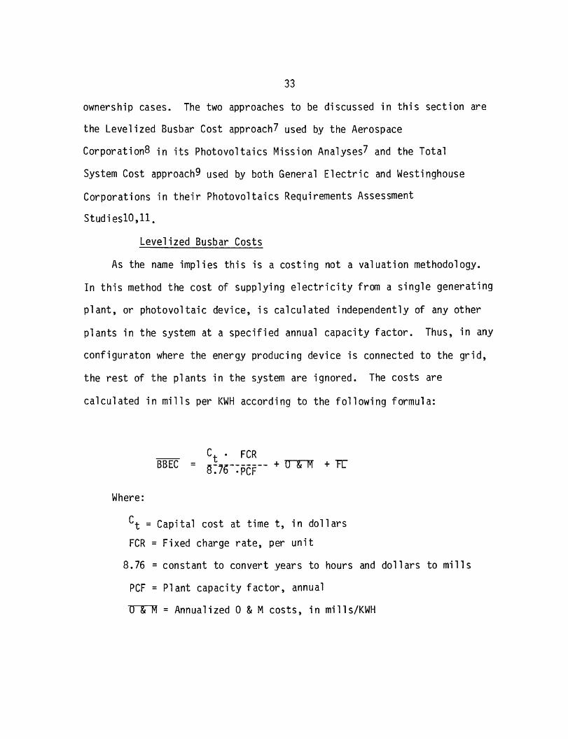
As the name implies this is a costing not a valuation methodology.
In this method the cost of supplying electricity from a single generating
plant, or photovoltaic device, is calculated independently of any other
plants in the system at a specified annual capacity factor. Thus, in any
configuraton where the energy producing device is connected to the grid,
the rest of the plants in the system are ignored. The costs are
calculated in mills per KWH according to the following formula:
Ct . FCRBBEC : P + &
Where:
Ct = Capital cost at time t, in dollars
FCR = Fixed charge rate, per unit
8.76 = constant to convert years to hours and dollars to mills
PCF = Plant capacity factor, annual
0 & M = Annualized 0 & M costs, in mills/KWH
34
FT = Annualized fuel costs, in mills/KWH
(Fr would be zero for photovoltaic plants)
Notice that this is not an economic valuation measure as we have defined
the term. It allocates capital costs over a specified lifetime implicit
in the fixed charge rate. The performance characteristics of the plant
are contained within the single plant capacity factor number.
There are a number of reasons why levelized busbar cost is an
inadequate methodology for the economic comparison of two methods of
supplying electricity. First, in order to be valid the capacity factors
must be the same for the two systems being compared. Capacity factor is
defined as the ratio of the average load on a machine or equipment for
the period of time considered, to the rating of the machine or
equipment. Thermal power plants have capacity factors lower than 100
percent due to unexpected or planned system outages. Photovoltaic plants
generally have very low capacity factors since here the capacity factor
is a function of sunshine availability. "It is impossible therefore for
a (photovoltaic) plant to have a capacity factor as high as the highest
of conventional thermal plants..."12 Of course, comparisons could be
made over a range of capacity factors, holding them the same for both
plants, but even this would not allow one to choose the appropriate
systems because the answer will change as the capacity factor changes.
Second, busbar costs do not account for the "effective" capacity of
the two plants. Effective capacity has been defined as the amount of
35
conventional capacity that would be displaced upon the installation of a
photovoltaics plant of a certain rated capacity. This is related to the
discussion earlier where it was argued that photovoltaic energy has a
"quality" component related to the time of day. "The insolation tends to
be available at a time in the daily work cycle when the loads are
highest; and depending upon the relationship of the timing of the
insolation peak and the daily load peak, (photovoltaic plant) effective
capacity can be considerably higher than capacity factor."1 3
Finally, busbar costs do not place a valuation on the impact of the
power plant on the total utility system. It is never the case that one is
just comparing a photovoltaics plant with a coal plant, in isolation. A
photovoltaics plant will behave very differently with respect to the
utility system when it is installed than would a coal plant, even if they
had the same capacity factor. Thus, busbar cost is not a sufficiently
detailed method to determine the value of a photovoltaic system to its
utility owner. It is also questionable whether the results it gives even
allow the decision-maker to make rough-cut, technology rankings.
Total Utility Systems Cost
In contrast to busbar cost, which is a purely analytic method, Total
Utility Systems Cost is a method that relies upon simulation. As we
shall see, this method, when implemented correctly, is the type of
analysis needed to perform the economic valuation of photovoltaics from
the utility point of view. If the photovoltaic system is utility-owned,
then we can stop here. If the systems are user-owned, however, total
36
systems costs provides only one part of the ultimate analysis (see
Section 6.4).
The Total Systems Cost Methodology involves a detailed hourly
stochastic simulation of the utility system reliability. This is
accomplished in terms of the widely-used expected value of systems outage
known as the loss of load probability (LOLP). The economic valuation of a
photovoltaic plant is calculated based on its ability to contribute to
the overall generation system reliability. A photovoltaic plant is added
to a "base" utility system, its output being considered a negative load
on the system, and conventional capacity is retired from the system until
reliability returns to its base LOLP value. This amount of conventional
capacity "displacement" is referred to as the photovoltaic plant
"effective capacity". The economic valuation is completed by summing the
value of the fuel costs displaced and the value of this effective
capacity. In order to assess the energy displacement characteristics of
a photovoltaic plant it is necessary to analyze the entire utility
generation system operation through a production cost simulation model.
This model dispatches generating capacity to meet the total system load
at minimum cost. Since the photovoltaic plant output is sunlight
dependent ("run-of-the-sun"), it must first be modeled and then the rest
of the utility plants are dispatched around it in the simulation.
Running the simulation with and without the photovoltaic plant addition
yields a valuation which includes both the displaced conventional
37
capacity and the displaced energy all at constant system reliability.1 4
This approach was used successfully by General Electric in their
Requirements Assessment of Photovoltaic Electric Power Systems1 4 to
show that photovoltaic plants did not necessarily require 100 percent
conventional capacity backup, as was widely asserted by many
commentators. There are, however, several necessary conditions that must
be accounted for in this methodology, conditions that General Electric
did not meet in their study:
A) The solar insolation data which determines the output of the
photovoltaic plant must be matched on an historical basis with the
utility system load data. This could be especially critical for
summer-peaking utilities where the presence of sunshine will increase the
air conditioning load. Energy demand and insolation are not independent
variables.
B) This methodology is not sufficient by itself for dispersed,
utility-owned systems. Explicit consideration must be taken of
transmission-distribution loss and reliability improvements that will be
enjoyed with dispersed photovoltaic systems.1 5
C) As alluded to earlier, the use of the total utility system cost
methodology by itself to calculate the economic value of photovoltaic
systems implies necessarily that utilities own the systems.
In the next section a methodology will be suggested that calculates
the economic value of user-owned photovoltaic plants.
BECC can be considered an economic indifference value - that price at
which the user would be economically indifferent between having and not
having the device. This formula contains a number of features. First,
the valuation which is the difference in the utility bills to the user,
is determined by the utility rate structure and whatever the utility is
willing to pay for surplus energy supplied by the owner to the grid. If
the rate structure reflects the load demand on the utility (as under
peak-load pricing), then this valuation explicitly values the "quality"
component of the energy supplied by the device. Second, it is a figure
defined in dollar units. This automatically adjusts for the scale of the
device and allows direct comparison between two devices in the same
application.
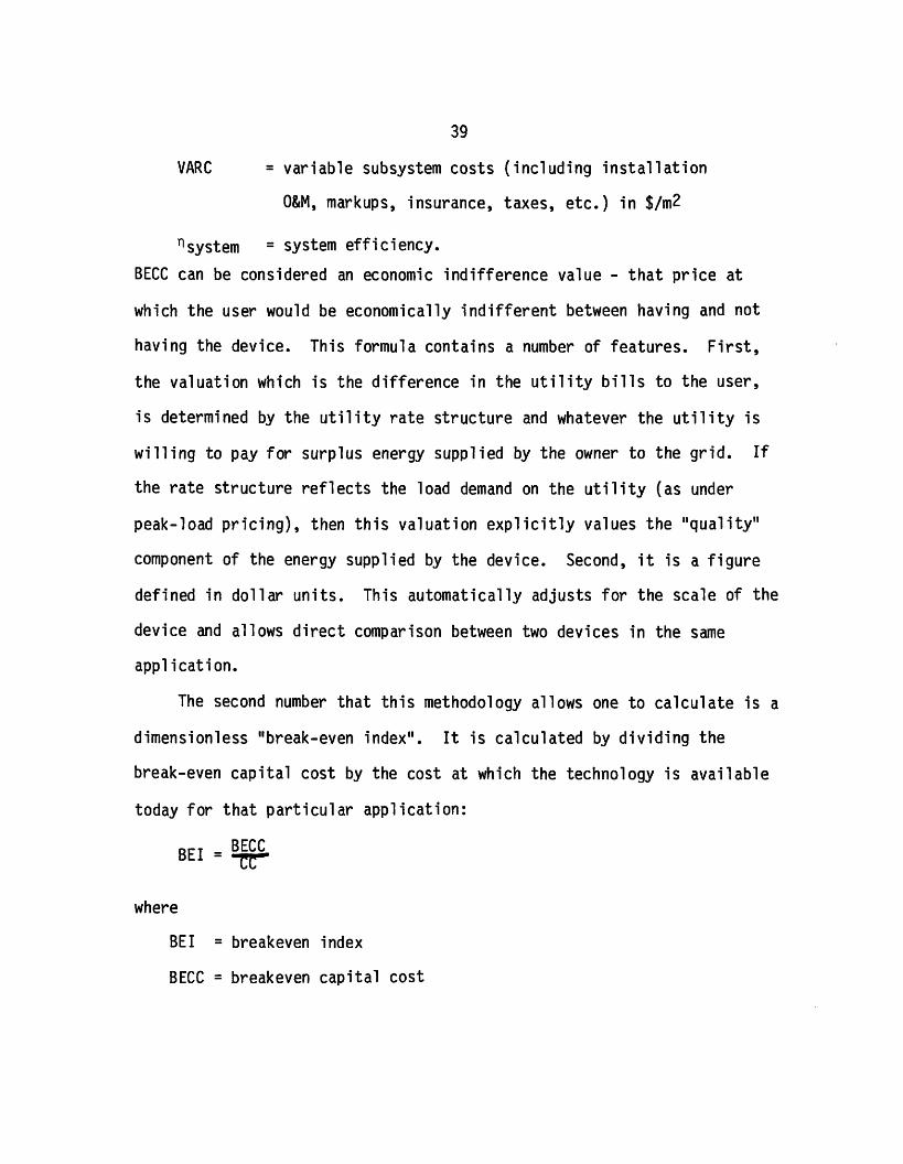
The second number that this methodology allows one to calculate is a
dimensionless "break-even index". It is calculated by dividing the
break-even capital cost by the cost at which the technology is available
today for that particular application:
BEI = BECC
where
BEI = breakeven index
BECC = breakeven capital cost
40
CC = current capital cost.
This measure is an attempt to implement in a simple manner the
demand-side, supply-side interaction mentioned earlier. The numerator,
BECC, constitutes the demand-side benefit measure while CC represents the
supply-side cost measure which indicates availability.
In a situation where future costs (CC) were perfectly known, this
index would allow one to compare different technologies in the same
application (what the busbar energy cost figure claims to do). BEI
would, under these circumstances, tell the investment decision-maker "how
far away" the technology is from break-even. Unfortunately, CC is not
known with certainty, and thus this measure is also imperfect. But by
introducing judgements as to possible future supply costs with
probabilistic distributions around these costs, it may be possible to use
this index for technology comparison. 1 6
While there is a fine line between what one would call an analytic
model and a simulation model, the fact that this methodology requires
hour-by-hour analysis suggests the necessity of simulation.
41
2.6 FOOTNOTES
1. General Electric Co., Requirements Assessment of PhotovoltaicElectric Power Systems, RP 651-1 for EPRI by GE Electric UtilitySystems Engineering Dept., Schenectady, NY, Draft Final Report, June1, 1977.
2. H.H. Marvin, Letter to Photovoltaic Program participants on"Photovoltaic Program Plan Restructure," August 5, 1977.
3. Dale D. Myers, Quoted in The New York Times, December 5, 1977, p. 61.
4. For discussion of the photovoltaics purchase decision and amethodology to measure the factors involved, see: Gary L. Lilien,The Diffusion of Photovoltaics: Background, Modeling and InitialReaction of the Agricultural-Irrigation Sector, MIT Energy LaboratoryReport MIT-EL 76-004, Cambridge, MA, March 1978.
5. Amory Lovins, Soft Energy Paths, Ballinger Publishing Company,Cambridge, MA, 1977, p. 69.
" Since we are obliged to begin committing resources now tothe long-term replacement of historically cheap fuels, we mustcompare all potential long-term replacement technologies witheach other, not with the cheap fuels, in order to avoid aserious misallocation of resources." (emphasis in original)
6. Work is currently under way to analyze this load aggregation problemby Prof. Fred C. Schweppe et al. of the MIT Electric Power SystemsEngineering Laboratory.
7. J.W. Doane, et al., The Cost of Energy from Utility-Owned SolarElectric Systems, JPL/EPRI-1012-76/3, Jet Propulsion Laboratory,Pasadena, CA, June 1976.
8. Aerospace Corporation, Mission Analysis of Photovoltaic Solar EnerConversion, for ERDA/Sandia, JAN/1101-77/1, March 1977.
9. C.R. Chowaniec, P.F. Pittman, D.W. Marshall, "A ReliabilityAssessment Technique for Generating Systems with Photovoltaic PowerPlants," IEEE PAS, April 21, 1977.
10. General Electric Co., op. cit.
11. Westinghouse Electric Co., Utility Assessment of PhotovoltaicElectric Power Systems, Follow-on Project under ERDA Contract
42
E(11-1)-2744 "Conceptual Design and Systems Analysis of PhotovoltaicPower Systems," 1977.
12. General Electric Co., op. cit., p. L-3.
13. Ibid., p. L-4.
14. For a more detailed description of the total systems cost
methodology, see GE, op. cit., Appendix F.
15. The so-called residential shingle scenario studied by GeneralElectric is a misnomer, because no effort was made to model thetransmission-distribution system. The answer would have been thesame if all of the dispersed shingles had been aggregated in acentral power plant, except for differences in subsystem costs.
16. It must be emphasized that this index provides only a part of the
information necessary to make R&D investment choices and decisions.No one measure can make these decisions in isolation since it isnecessary to understand how alternative R&D budget allocations affectfuture technology development along many dimensions. The claim ismade, however, that knowledge of the point at which technologiesreach economic "breakeven" in the marketplace is a vital piece of theinformation that is needed.
43
III. SIMULATION MODEL DESCRIPTION AND INPUT ASSUMPTIONS
3.1 REGIONAL DEFINITION
The choice of regions in which to perform the analysis is based on
the work of Carpenter and Tabors.1 This regional definition study was
performed in recognition of the fact that most existing regional schema
for energy analysis are not well suited to data collection 2 or are
improperly constructed to reflect solar energy and climatic
characteristics. The methodology employed by this analysis was a
multivariate statistical method called two-stage factor analysis coupled
with cluster analysis of cases. Using states as regional building
blocks, this methodology examines groups of variables and their
correlations and based on these correlations constructs linear
combinations of variables, called factors. This technique isolates the
underlying dimensions in the data and allows one to condense many
variables into a few "factored" variables. Each state has a
corresponding score for each of these factors and these factor scores are
then used by the cluster analysis to group similar states and
differentiate dissimilar states. Homogeneous regions are thus
constructed based on many underlying variables.3 Figure 2 is a box
diagram depicting this two-stage process. As indicated, the data set
consisted of 8 climate variables representing solar radiation
availability and heating and cooling requirements, 10 economic variables
measuring energy consumption, income, value added and growth, and 12
A A
~cl)U).J(ac(M v,
Cl)
(I)~
w cr5W , cr&LJ(3scnQ- Q
Z0Izo
~LLFOLLZ
-JZ
0o _dat w c- ),
o I- zzo0
wCl)
0
I-
.I0n
0O~ I
45
production-supply variables reflecting fuel prices, refinery capacity and
energy pruduction.
The final regional breakdown is illustrated in Figure 3. Because of
their homogeneity, each region can be unabiguously defined based on the
final factors which are linear combinations of the above variables. For
example, Region V, the Southwest, is characterized by high consumption,
sunny climate, affluence and high energy prices. (See Carpenter and
Taborsl (1978) for a more detailed summary and quantitative description
of the regions). Due to time and data limitations, three of these seven
regions were selected for the analysis presented in this document; those
regions which include Boston, Omaha, and Phoenix. It was felt that these
three areas provided a sufficiently broad cross-section to be
representative of typical results for all regions.
3.2 VALUATION MODEL
The model employed to value PV systems in this study can be
conceptualized as three separate models: A) a photovoltaic array
simulation model B) a load-scheduling simulation model, and C) an
economic valuation model.
PV Array Model
This model provides an application and location-specific simulation
of the output of a photovoltaic system. Specific system configurations
are input by means of design parameters such as array size, packing
factor, efficiency, loss factors, array tilt, etc. Location specificity
CC
ECC
uj
LL
1! i -
47
is achieved by the designation of latitude and the use of local data for
insolation and temperature. Thus, given system configuration, latitude,
and hourly weather data, the simulation provides hourly PV system (i.e.
conditioned A/C) electric power levels.4
Load-Scheduling Model
Residential usage of electricity is determined on the basis of
appliance load and electricity price inputs and the availability of
electricity from the solar array model. Appliance energy consumption and
use assumptions are input to the model in the form of vectors described
below in Section 3.3.3. Price information is in the form of utility rate
structures. Output from the array simulation determines the availability
of photovoltaic energy.
Scheduling is accomplished through a process intended heuristically
to optimize use of the PV array output. 5 Each half-hour the scheduling
heuristic proceeds through five steps summarized in Figure 4, first
constructing a prioritized list of loads with "must run" loads at the top
and other "runnable" loads in descending order of total cost. 6
Available PV system output is then dispatched to cover as many of the
loads as possible. If array output is more than needed to cover all the
"runnable" loads in a period, excess is sold back to the utility grid at
a designated price. When solar electricity is insufficient to cover the
entire list, the remaining loads are postponed except for those
designated "must run," which are then scheduled using electricity
48
Figure 4
SIMULATION MODEL SCHEDULING HEURISTIC
1. IS LOAD IN MUST-RUN PERIOD? RUN THOSE LOADS THAT MUST BE RUN.
2. IS LOAD "RUNNABLE"? A LOOK-AHEAD IS PERFORMED FOR RUNNABLE LOADS
WHICH ATTACHES COSTS TO THE LOADS IN VARIOUS RUN SCENARIOS BASED ON
THE AVERAGE UTILITY PRICE OVER THE RUN PERIOD. LOADS ARE RANKED IN
ORDER OF MOST EXPENSIVE AND, IF THERE ARE TIES, BY LARGEST LOAD.
3. IS THERE SOLAR AVAILABLE? RUNNABLE LOADS ARE SWITCHED ON IN
PRIORITY ORDER WHILE EXCESS SOLAR EXISTS. IF INSUFFICIENT SOLAR
EXISTS TO COVER FULL LOAD THEN LOAD IS SWITCHED ON WHILE THE
WEIGHTED PRICE OF SOLAR PLUS UTILITY POWER IS LESS THAN A PRE-SET
LIMIT.
4. LEFT-OVER SOLAR IS SOLD BACK TO UTILITY.
5. IF NO SOLAR THEN LOADS OTHER THAN "MUST-RUN" ARE POSTPONED.
49
purchased from the utility grid at the price (determined by the rate
structure) prevailing for that particular time period. Records are kept
accounting for all PV output and all electricity purchased from the
utility, as well as the total utility bill incurred and what that bill
would have been had consumption remained unchanged and had all energy
been purchased from the utility grid.
Economic Model
The economic valuation model performs two functions. The first is
necessitated by the fact that the first two sections described above,
which simulate the PV residence, are run for only a single year. Since
these single-year reslts would not be expected to remain stable through
time, evaluation requires that the one-year figures be projected over the
lifetime of the system. This is accomplished by applying degradation7
and fuel escalation8 assumptions through time to develop a twenty-year
profile of PV benefits. The second portion of the model simply performs
a net present value calculation by the application of a discount rate to
yearly energy savings* to arrive at a gross market breakeven value.
Subsystem, operation and maintenance, shipping and distribution, and
other relevant costs 9 as well as profit margins etc. are then
*It should be mentioned here that the utility bill with solar was
compared to the time-of-day bill that would have resulted without solar.This was done to assure that savings resulting from behavioral shiftsmotivated by the time-of-day structure alone were not capitalized intothe value of the PV system.
50
subtracted to arrive at the net breakeven figures presented. See formula
in Section 2.5 and computer program in Appendix C. The input assumptions
and sensitivity analysis scenarios for the economic valuation model are
presented in Chapter IV.
3.3 MODEL INPUTS
The following sections describe the specific assumptions and data
inputs for each segment of the array and load scheduling models described
above.
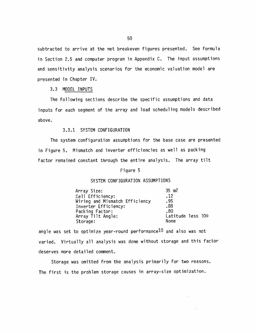
3.3.1 SYSTEM CONFIGURATION
The system configuration assumptions for the base case are presented
in Figure 5. Mismatch and inverter efficiencies as well as packing
factor remained constant through the entire analysis. The array tilt
Figure 5
SYSTEM CONFIGURATION ASSUMPTIONS
Array Size: 35 m2
Cell Efficiency: .12
Wiring and Mismatch Efficiency .95Inverter Efficiency: .88Packing Factor: .80
Array Tilt Angle: Latitude less 10oStorage: None
angle was set to optimize year-round performance1 0 and also was not
varied. Virtually all analysis was done without storage and this factor
deserves more detailed comment.
Storage was omitted from the analysis primarily for two reasons.
The first is the problem storage causes in array-size optimization.
51
Without marginal cost functions for array and storage equipment it was
not possible strictly to optimize the PV system. It was hoped that over
the range of array sizes relevant to the residential application there
would be a peak in the per unit net breakeven value 11l ($/m2) which
would proxy as an optimum assuming constant cost per m2 of array.1 2
The inclusion of storage would have made such a determination much more
complex. A much more serious problem which provided the second reason
for storage exclusion is the fact that benefit allocation becomes more
difficult when storage is included. Since storage can reduce electricity
bills given a time-of-day pricing structure with or without a PV
array,1 3 the benefits to a combined system could accrue to the PV
array, to the storage, or to the interaction of the two. This allocation
difficulty underscores the fact that photovoltaics and storage, rather
than being complementary as is commonly believed, appear in fact to be
competitive or substitute devices for grid-interfaced systems.1 4
Both array size and cell efficiency have been varied from the base
case in parametric analysis. The 35 m2 array size was in fact selected
as the base size because of its apparent optimality, given location and
buy-back rate possibilities (see Section 5.1) in the sensitivity runs.
The range on size, 5-85 m2, covers those thought reasonable in
residential applications. Cell efficiency was set at .15 on sensitivity
runs because, while present efficiencies are around .12, the higher
figure is projected cell performance for 1986.15
52
3.3.2 INSOLATION DATA
Historically, hourly solar radiation data have suffered from neglect
and have contained serious errors resulting from gaps in collection and
calibration and instrumentation problems. Recently, these data have been
rehabilitated for 27 of the weather stations across the country and have
been formated with other hourly meteorological measurements in the
so-called Solmet format, now available on magnetic tape from the National
Climatic Center of the National Oceanic and Atmospheric
Administration.16
While the quality and amount of data vary from station to station,
most of the stations for which there is Solmet data report at least 15
years of historical hourly solar radiation data.
Since it was hypothesized that the simulation valuation would depend
heavily on the amount of solar radiation in a given year, care was taken
to define "typical," "best," and "worst" years for solar radiation in
each of the three areas analyzed.1 7 Because each tape contains
approximately 175,000 individual hourly readings for each city, analysis
of variance using available statistical routines proved intractable. And
while it would be ideal to have a summary statistic concerning insolation
variation on an hour-by-hour basis, the extreme volume of information to
be analyzed made its analysis beyond the scope of this study. Instead, a
set of computer programs was designed (see Appendix B) to compute and
analyze the variation in monthly-hour insolation averages. This involved
53
the creation of a 12 x 24 matrix for each year relating average
insolation by hour of the day to month of the year. Each corresponding
cell of the yearly matrices were then analyzed for variation and the year
whose monthly-hour averages were most similar to the mean year was
selected. This method is crude in the sense that variation within any
particular month is washed out, but on the other hand it does allow one
to select objectively a typical year based on some global criteria.
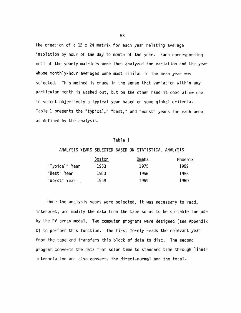
Table 1 presents the "typical," "best," and "worst" years for each area
as defined by the analysis.
Table 1
ANALYSIS YEARS SELECTED BASED ON STATISTICAL ANALYSIS
Boston Omaha Phoenix
"Typical" Year 1953 1975 1959
"Best" Year 1963 1966 1955
"Worst" Year 1958 1969 1960
Once the analysis years were selected, it was necessary to read,
interpret, and modify the data from the tape so as to be suitable for use
by the PV array model. Two computer programs were designed (see Appendix
C) to perform this function. The first merely reads the relevant year
from the tape and transfers this block of data to disc. The second
program converts the data from solar time to standard time through linear
interpolation and also converts the direct-normal and the total-
54
horizontal insolation measurements to direct and diffuse insolation on a
horizontal surface through standard geometry.1 8
3.3.3 APPLIANCE LOADS AND BEHAVIORAL ASSUMPTIONS
Figure 6 summarizes the appliance loads and use patterns which were
scheduled in the simulation model. Appliance ratings (power
requirements) and yearly consumption figures (energy usage), excepting
those for lighting1 9 and air conditioning,20 were taken from data
compiled by General Electric Co. for their study titled Conceptual Design
and Systems Analysis of Photovoltaic Systems.2 1 Division of yearly
consumption by appliance ratings yielded hours of use on a yearly basis.
Hours of use were then distributed on a daily and weekly basis so as to
reasonably approximate normal usage.
The figures for the refrigerator, for example, indicate
1829 KWh/615W = 2974 hours of use per year for an average of slightly
over 8 hours per day. People obviously do not turn their refrigerators
off for 16 hours a day so this implies that the thermostatic control of
the unit causes it to operate in on/off cycles in which the unit is
"running" (drawing energy) about one-third of the time. For the
remainder of the cycle the unit is automatically placed in a "hold" mode
which uses no (or negligible) energy. Consequently the refrigerator has
been modeled as if it ran 20 minutes each hour.2 2 This results in a
very static load which cannot be shifted to any significant degree. The
scheduling routine in the simulation can move the 20-minute "on" period
55
Figure 6
APPLIANCE USE AND BEHAVIORAL ASSUMPTIONS
Load # Appliance Rating YearlyConsumption
Refrigerator 615W
2& 3
4& 5
Dryer
Washer
6 Water
heater
Range loads
7. Dinner8. Lunch9. Breakfast
4850W
500W
2500W
9100W2400W2700W
1829kWh
1008kWh
103kWh
4270kWh
1205kWh
Unit is on continuously
but draws load (i.e. isrunning) only one-thirdof the time to maintain
proper temperature(runs only 20 min. eachhour).
Eight half-hour loads.May be run at any time
during day/night butfour loads must be runin each half of eachweek.
Same as dryer.
Unit is on from 6 a.m.
to midnight but runsonly one-fourth of eachhour to maintaintemperature.
Meal loads representdifferent combinationsof oven, broiler, and
range-top burners thatmight be used for each
meal. Each load is 30min. in duration.Breakfast, lunch, anddinner start times are
6-7:30 a.m., 11:30-12:30 p.m., and 6-8p.m., respectively.
1
Comments
56
Figure 6
APPLIANCE USE AND BEHAVIORAL ASSUMPTIONS (continued)
Load # Appliance
10 TV
Rating
200W
YearlyConsumption440kWh
CommentsUnit runs for 6 hoursper day beginning inthe late afternoon or
early evening.
Dishwasher
Lighting
Central AirConditioning
1250W
2400W
5000W
363kWh
1314kWh
Variable
Runs consist of two30-min. or one 1-hourcycle each day. Maybe run after eitherbreakfast or dinner.
Lighting for a 6-7room home. Roughlyone-fourth of thelights are on at any
time during eveninglighting hours.
A/C mode is triggeredby two days with
temperatures greaterthan 2 5.5oC. Oncein A/C mode unit isturned on when tempera-ture reaches 2 1.9 oCand runs continuouslyuntil house is cooledto 20.9oC.
11
12
13
57
within each hourly cycle.
Other loads are much more flexible. The clothes dryer is used
1008kWh/4850W = 207 hours per year or about 4 hours per week. This
represents eight 30-minute loads which need not be run at any particular
time. Therefore the only constraint placed upon these loads is that they
not be run all on the same day. This was accomplished by requiring four
loads to be run in each half of a weekly cycle. Because of the technical
design of the simulation model this required the use of the two separate
dryer loads which appear in Figure 6.23
Once characterized as in Figure 6, load and behavioral information
for each appliance was input to the model by means of a 24-entry vector
like those shown for the refrigerator and dryer in Figure 7. The second
and twelfth entries contain the appliance rating and cycle length
discussed earlier. Entries 3 and 4, along with the cycle length, define
energy consumption and represent average consumption while "on" and the
run duration respectively. For the refrigerator these entries indicate
that each hour (entry 12) the unit must run for one half-hour (entry 4)
at an hourly consumption rate of 420W (entry 3). Thus each hour the
refrigerator uses 420W x 0.5 hr = 210 Wh of energy. 2 4 Other entries
control when and how often a load can be interrupted (5-11), how much the
load's scheduled start time (identified in entry 13) can be advanced (14)
or delayed (15) and what percentage of the time the load can be foregone,
or avoided altogether (16, 17).25 The remaining entries are
essentially bookkeeping locations for the computer.
58
Figure 7
SAMPLE APPLIANCE LOAD VECTORS
Refrigerator
Dryer #1
Refrigerator
Dryer #1
Refrigerator
Dryer #1
1 2 3 4 6 7 8 9 10
1.0 615 420 0.5 0 0 0 0 0
1.0 4850 4850 2 28 0 24 0 4
11 12 13 14 15 16 17 18 19
0 1.0 0 0 0.5 1.0 1.0 5 3
0 168 -143 24 24 1.0 1.0 5 5
20 21 22 23 24
0 0 0 0 0
o o 0 o 0
59
3.3.4 RATE STRUCTURES
Energy delivered by the photovoltaic system simulated was valued
through applicaton of time-of-day rates which reflect marginal costs for
each of the utility systems studied. While none of the utilities
presently charges consumers on the basis of such rates, they have been
used in the analysis because they more accurately reflect energy costs
both to the utility companies and society at large than do present block
rate structures. Utility companies, threatened by the rapid rise in
electricity production costs2 6 and consumer resistance to spiraling
utility bills,2 7 have become cognizant of the fact, long recognized by
economists, that rate structures which do not accurately reflect
electrical production costs28 present price signals to consumers which
lead to inefficient resource allocations. This inefficiency has
evidenced itself in declining load factors2 9 and rising reserve
margins.30 The falling utilization of capacity is caused by the fact
that peak demand is growing faster than average demand,3 1 a phenomenon
which can be attributed to block rates which essentially undercharge peak
users and overcharge off-peak users.3 2 The use of time-of-day rates
based upon marginal costs avoids capitalizing economic distortion
inherent in declining block structures into the valuation of the PV
system and furthermore, time-of-day rates are what the PV system owner of
the future is most likely to encounter given current utility industry and
governmental initiatives.3 3
60
The rates used in the simulation were developed through a two-step
process. First marginal generating costs were determined for each of the
utilities studied. The second step occurred after initial simulation
runs and consisted of adjusting the rates up or down to equalize the
bills that time-of-day and declining block structures produce for
consumers with similar consumption levels.
Marginal costs for the New England Electric System and for Arizona
Public Service were those derived by Feldman and Anderson34 for their
solar space conditioning (SHAC) study. Costs were derived for the Omaha
facility using the "peaker" method similar to that outlined by Cicchetti
and Gillen in their study of the Central Maine Power Company35 which
consists of three basic steps described below.
1. Marginal Generating and Transmission Costs
First the marginal generating unit is identified. Here, as in most
utilities, the marginal generating unit is a 50 MW gas combustion
turbine. The per KW installed cost of the unit is adjusted for outage
rate and annualized by application of a capital recovery factor and added
to annual operation and maintenance costs per KW to arrive at a total
yearly cost per KW generated. This figure is adjusted upward to cover
reserve margin and line losses to develop a generating capacity cost per
KW used by the consumer. To this generating capacity cost are added
marginal transmission and distribution costs3 6 to get a total capacity
cost per KW consumed at the margin.
61
2. Determination of Pricing Periods
Since capacity costs must be spread over those periods in which
demand taxes the utility's generating equipment, it is necessary to
identify such periods. The ideal way to make such a determination is to
select those periods with significant loss-of-load probabilities (LOLP -
the expected value of system outage) as peak or shoulder periods. Data
for these determinations, EPRI's Synthetic Electric Utility Systems for
Evaluating Advanced Technologies,3 7 however, did not provide LOLP
information. Since LOLP is related to system load38 it is possible to
make the allocations based upon hourly loads which were available.3 9
Once capacity costs and rate periods have been determined the capacity
costs applicable to each period are merely divided by the number of hours
in the period to arrive at a kWh rate for capacity in each period.
3. Calculation of Period Energy Costs
This consists of selecting the relevant (most costly to operate)
unit in each of the rating periods, which, along with the combustion
turbine "peaker" included a 200 MW oil unit in the shoulder period and a
400 MW coal-fired plant during the base or off-peak period, and then
using the applicable fuel costs and heat rates for these machines to
arrive at cost per kWh generated. This is adjusted for line losses to
arrive at a cost per kWh delivered to the end user. Heat rate data were
taken from the EPRI Synthetic Utility data, and Nebraska fuel prices were
found in the Edison Electric Institute's Statistical Yearbook, 1976.40
62
Costs per kWh for capacity and energy are then summed for each
period to arrive at the marginal cost. Rates used for each utility
simulated are summarized in Tables 2-4. These rates are not strictly the
marginal costs calculated above but rather the marginal costs adjusted in
the second step of the procedure mentioned earlier. This adjustment was
necessary for two reasons. First, our method of calculating marginal
costs ignored what are often called consumer-related charges such as the
cost of metering, etc. Second, adjustment was thought to be necessary to
assure that utility revenues would not fall or rise substantially in the
short run. Since the utility companies' capital commitments would not be
altered in the short run because of a shift to a time-of-day rate, their
revenue requirements to cover expenses, investor return, etc. would also
be unaltered. Marginal costs are determined without regard to revenue
requirements, and thus rates based solely upon marginal costs might
result in short-run revenue deficiencies.41
In order to make the necessary adjustment the simulation model was
run with a rate structure reflecting only marginal costs. On this basis
a utility bill for the simulated owner's entire energy consumption (this
required pricing of the energy used from the PV system as if it were
purchased instead from the utility company) was calculated and compared
to the typical utility bill for a customer of the same utility company
(based on existing declining block rates) in a comparable monthly
consumption range as reported in the FPC's Typical Electric Bills,
63
Table 2
BOSTON TIME-OF-DAY RATE STRUCTURE
Total Price (/kWh)
Capacity
Fuel
Peak
6.73
4.04
2.69
Year-Round:
Weekdays
Weekends
Holidays
Peak
7 a.m. - 9 p.m.
Base
10 p.m. - 6 a.m.
All day
All day
Base
2.60
.32
2.28
64
Table 3
OMAHA TIME-OF-DAY RATE STRUCTURE
Peak Shoulder Base
Total Price (.kWh) 4.70
Capacity 3.36
Fuel 1.34
Spring: 3/1 - 5/31 Peak
2.26
0.67
1.59
Shoulder
Weekdays
Weekends
Holidays
7 am - 12
7 am - 12
7 am - 12
Summer: 6/1 - 8/31 Peak
m
m
m
Shoulder
1 am - 6 am
1 am - 6 am
1 am - 6 am
Base
10 am - 9 pm 8 am - 9 am,
10 pm - 12 m
8 am - 12 m
8 am - 12 m
I am - 7 am
1 am - 7 am
1 am - 7 am
Winter: 9/1 - 2/28 Peak
9 am - 10 pm 6 am - 8 am,
11 pm - 12 m
6 am - 12 m
6 am - 12 m
1 am - 5 am
1 am - 5 am
1 am - 5 am
0.84
0.00
0.84
Base
Weekdays
Weekends
Holidays
Weekdays
Shoulder Base
Weekends
Holidays
65
Table 4
PHOENIX TIME-OF-DAY RATE STRUCTURE
Peak B
Total Price (/kWh)
Capacity
Fuel
Winter: 11/1 - 3/31
20.05
16.82
3.23
Peak
Weekdays
Weekends
Holidays
Summer: 4/1 - 10/31 Peak
2 pm - 5 pm 6 pm - 1 pm
All day
Holidays
2
ase
.43
.38
2.05
Base
All day
All day
All day
Base
Weekdays
Weekends
All day
66
1976.42 If the simulated bill was below (above) the typical bill the
rates were adjusted upward (downward), while maintaining constant
period-to-period price ratios, so that the bills were equalized. Figure
8 presents the adjustment formula and Figure 9 demonstrates the
adjustment calculation for the Boston rate structure.
67
Figure 8
FORMULA FOR REVENUE RETURN EQUALIZATION
DATA: TB = ¢/KWH (TYPICAL ELECTRIC BILLS FOR JANUARY FOR A
1. Carpenter, Paul, and Tabors, Richard, Solar Photovoltaic PlanningRegions, MIT Energy Laboratory, Cambridge, MA (forthcoming).
2. For example, the National Electric Reliability Council electricpower regions are hopelessly gerrymandered, cutting across numerousstate boundaries.
3. For a detailed description of the theory underlying factor analysisand its use, see R.J. Rummel, Applied Factor Analysis, NorthwesternUniversity Press, Evanston, IL, 1970.
4. This model was adapted by Jesse Tatum of the MIT Energy Laboratoryfrom the array model developed by General Electric Co. in theirstudy, Requirements Assessment of Photovoltaic Electric PowerSystems, RP-651-1 for Electric Power Research Insitute, FinalReport, June 1977.
5. This is not an optimization in the strict sense, which would requirea weather-forecasting capability, but rather a simple procedure tomake reasonably efficient use of the solar electricity.
6. A load's condition (i.e. "runnable," "must run" etc.) is determinedby behavioral parameters in the load vector (discussed below) andwhether or not the load has already been supplied.
7. These assumptions are described in detail in Section 4.1.
8. These assumptions are described in detail in Section 4.1.
9. Subsystem cost assumptions are outlined in Section 4.3.
10. Boes, E.C. et al. Availability of Direct, Total, and Diffuse SolarRadiation to Fixed and Tracking Collectors in the U.S.A., SandiaLaboratories, Report No. SAND77-0885, 1977.
11. It must be remembered that the "net" figure has all fixed subsystem
costs removed, an unfortunate reliance on estimated costs.
12. This seems an entirely reasonable assumption over the narrow rangeof relevant array sizes.
13. By charging storage at low rates (i.e. off-peak) and using the
energy to displace expensive peak consumption.
70
14. This relationship would persist so long as both are competing as
peak-shaving devices. Should PV ever compete as baseloadgeneration, storage would become a complementary device.
15. U.S. Department of Energy, Division of Solar Technology, National
Photovoltaic Program Plan, Washington, D.C., February 2, 1978, p. 18.
16. National Oceanic and Atmospheric Administration, U.S. Department of
Commerce, Hourly Solar Radiation - Surface MeteorologicalObservations SOLMET Vol. 1 - User's Manual, NOAA Environmental DataService, Asheville, N.C., December 19//.
17. While typical insolation years were selected, no effort was made to
evaluate the typical years from a thermal or cooling perspective.There is some a priori reason to suspect that years with highinsolation would have high cooling requirements, but this certainlydepends on the region.
18. Equations taken from Boes, E.C., et al., op. cit.
19. Lighting loads were developed from information contained in FederalEnergy Administration, A Study of the Electric Utility IndustryDemand, Costs, Rates, Washington, D.C., Conservation Paper No. 53,July 1976, and Dole, Stephen H., Energy Use and Conservation in the
Residential Sector: A Regional Analysis, R-1641-NSF, RandCorporation, Santa Monica, CA, June 1975.
20. The air-conditioning load (unlike other loads) is simulated in themanner summarized in Figure 6 so that the load is dependent upon the
weather. Information on consumption and thermal integrity factorsfor residences used in the simulation was obtained from Dole,Stephen H., Ibid.
21. General Electric Co., Conceptual Design and Systems Analysis of
Photovoltaic Systems, G.E. Space Division for ERDA/Sandia,Albuquerque, NM, March 19, 1977.
22. Because of model limitations the unit was simulated to run one half
hour each hour at a rate lower than 615W to approximate the correct
consumption. See explanation in note 24 below.
23. See Section 3.3.3.
24. Since the smallest time increment recognized by the model was 30
minutes, it was not possible to directly schedule the 20 minute/hourload for the refrigerator discussed above. Scheduling for a
30-minute load at a lower consumption rate accomplishes the sameresult. 615W x 20+ min/hr 210 W/hr.
71
25. The "forego" option was not used for any of the loads used in this
study because its use implies energy conservation on the part ofconsumers (the obvious result of not using an appliance) and becausewe wanted to remain on the conservative side vis-a-vis consumerflexibility of consumption. The option could be used to simulatevery flexible consumers.
26. See Uhler, Robert G., Electric Utility Rate Design Study, RateDesign and Load Control, Palo Alto, CA, September 1977, Chapter 1,pp. 9-10.
27. Prices to consumers in the 500-1000 KWh/month range (average
consumers) have risen 85-90% from 1970 to 1976, or 10-11% per year.See Federal Power Commission, Typical Electric Bills, 1976,Washington, D.C., 1976, p. xi.
28. See Uhler, Robert, op. cit. Also Cicchetti, C.J. and Gillen, W.J.,A Marginal Coast Analysis for Electricity, A Case Study of theCentral Maine Power Co. for the Attorney General of Maine uner agrant from the New England Regional Commission, January 1977, pp.7-9.
29. Load factor is the ratio (expressed as a percentage) of average
demand to peak demand. The load factor for the utility industry hasdeclined fairly steadily from 64.1 in 1969 to 61.4 in 1975. SeeFederal Energy Administration, E;ectric Utility Rate DesignProposals, Washington, D.C., February 1977, p. 53.
30. Reserve margin is the ratio (expressed as a percentage) of unusedcapacity to peak load. U.S. utility reserve margins rose from 46.4to 50.0 in the period 1970-1976. See Uhler, Robert, op. cit., p. 15.
31. Federal Energy Administration, Electric Utility Rate DesignProposals, op, cit., p. 53.
32. Federal Energy Administration, A Study of Electric Utility Rates and
Demands, Costs, and Rates, op. cit., Sections I and II.
33. See the Energy Conservation and Production Act (Pub. L. 94-385)Title SS 203(a).
34. Feldman, S.L. and Anderson, B., Utility Pricing and Solar Energy
Design, Clark University, Worcester, MA, NSF/RANN-760406, September1976.
35. Cicchetti, C.J. and Gillen, W.J., op. cit., pp. 49-64.
72
36. Since transmission and distribution costs differ substantiallyacross classes of consumers, marginal T&D costs are normallycalculated by regressing new (as opposed to replacement) capacityinvestments against demand by consumer class over some historicalperiod to achieve proper classwise allocation of costs. This wasimpossible since the EPRI data (see note 37) had no historical cost
or demand information so T&D costs were simply estimated.
37. Electric Power Research Institute, Synthetic Electric Utility
Systems for Evaluating Advanced Technologies, prepared by PowerTechnologies, Inc. for EPRI, Palo Alto, CA, February 1977. Asynthetic utility approximating the Omaha system was used ratherthan actual data because time did not allow collection of the latterand only a reasonable facsimile of the appropriate rates wasnecessary.
38. The relationship is nonlinear with LOLP falling off very rapidly asload declines.
39. Demarcations were made at approximately 80% and 50% of yearly peakload for peak and shoulder periods respectively.
40. Edison Electric Institute, Statistical Year Book of the Electric
Utility Industry for 1976, 90 Park Avenue, NY 10016, October 1977.
41. Such deficiencies would be expected to disappear in the long run asshifting consumer demand patterns allowed more efficient use ofexisting plant and alteration of the generation mix itself.
42. Federal Power Commission, op. cit.
73
IV. ECONOMIC MODEL INPUTS AND SENSITIVITY ANALYSIS ASSUMPTIONS
4.1 FUEL PRICE ESCALATION AND CELL DEGRADATION RATE
The one-year results of the residential simulation were adjusted to
take into account rising electrical prices and declining cell output (or
degradation) over the life of the PV system. Forecasting future
electrical rates in utility systems is a difficult dynamic problem
discussed later in the study.l To avoid this problem a constant
utility generating mix has been assumed and rates have been projected by
applying a fuel-escalation factor to the portions of the time-of-day
rates which reflect fuel costs. The base case assumes that fuel costs
will climb at a 3% per year real rate (above inflation). For comparison
purposes runs were also done at a 0% real growth rate in fuel prices.
Cell degradation is a fairly unknown factor at this stage of PV
development.2 It is known that degradation occurs, but data are
insufficient to determine accurately its pattern over the array lifetimes
presently contemplated. For our base case calculations, available output
was calculated to decline 3% each year. Thus, at the end of the 20-year
period the array is delivering only about 56% of its original
performance3. The baseline results are thus fairly conservative. A
less conservative yet likely scenario,4 depicted graphically in Figure
10, was run as a comparison. In this version array output declines
rapidly in the earlier years (5% in the second and third years) and then
stabilizes with a very slow decline (.7% per year) thereafter so that the
0)
I'-
(0
O
nCM
30)
r,-
(D
Ln
N
74
OwllJ11D:
CD
0 0 0 0 0 00 0) NO) I- L t
OOiOV.I NOIV(V3Jg3]
75
array is producing approximately 80% of its original output after 20
years.
4.2 DISCOUNT RATE
Discounting of future costs or energy savings can be treated in
various manners. Studies concentrating on utility ownership scenarios
even though applications were dispersed5 have naturally relied upon
utilities "cost of capital."6 Residential studies have used the
mortgage interest rate as a discount rate.7 Some might argue that
since the ultimate concern of this study is government expenditure
policy, a social discount rate should be applied in comparing outlays and
benefits.8 Finally, current finance theory would suggest the use of
the investors' opportunity cost of capital as the appropriate rate.
The market indifference point methodology used in this analysis
eliminates consideration of both the utility cost of capital and the
social discount rates for valuation purposes. While the PV system is
utility-grid integrated, the homeowner is making the investment decision,
not the utility company. The utility cost of capital has no relevance.
A social discount rate is similarly irrelevant because the immediate
concern is not societal but rather individual investment decisions.
Understanding these individual investment decisions will, it is hoped,
shed light on governmental subsidy expenditure options which should be
evaluated on the basis of the social rate. For now, however, the
individual homeowner is the primary concern.
76
Studies to date of dispersed residential user-owned units9 have
employed the mortgage interest rate as a discount rate.10 The
justification for such an approach appears to be the assumption that this
would be the cost of capital to the homeowner in a scenario where the
solar investment is financed with a standard home mortgage as part of a
new-home purchase. Insofar as this approach relies upon the investor's
marginal borrowing rate to establish an opportunity cost, it is not
theoretically sound, because the investor's opportunity cost depends not
upon the source of funds but rather upon alternative uses. The
opportunity cost is the return that might be obtained through an
alternative investment with risk characteristics similar to the one under
consideration.ll Use of the mortgage rate would be justified, then,
only if the risks inherent in the PV investment 1 2 were identical to
those found in home mortgage investments generally.1 3 Thus we are
faced with the question of whether or not there are differential risks
between the two types of investment, or stated alternatively, whether or
not there are risks inherent in the PV investment which do not apply to
normal mortgage investments and which therefore imply use of some other
higher or lower opportunity cost as a discount rate.
Before pursuing this question any further a discussion of the nature
of risk and the risk/return relationship is in order. On an intuitive
level it seems obvious that investors would expect greater returns for
relatively riskier investments, i.e., as an investment becomes riskier,
77
investors will demand greater inducements (in the form of returns) to
hold on to the investment. Current finance theory has added two
refinements to this intuitive picture to derive a valuation formula for
investments called the capital asset-pricing model (CAPM).14 The first
refinement is simply a working definition of the concept of risk. Risk
is represented by the variance in the returns inherent in the asset or
assets underlying the investment. A risky asset then is one with a good
deal of uncertainty about its return due to a wide variation in possible
outcomes.1 5 The second deviation from the intuitive picture concerns
diversification and the separation of risk into two components called
systematic risk and unsystematic risk. Because uncorrelated variances
are not additive 1 6 it is possible to "diversify" away risk while not
sacrificing return by holding combinations or portfolios of assets or
investments.1 7 Since the investor can shed, or diversify away, risk at
no cost, current theorists reason that bearing "diversifiable" risk does
not command increased return.1 8 There is a limit, however, to risk
reduction through diversification.* Theoretically this limit is
exemplified by a portfolio containing all possible investments in
proportion to the ratio of their value to the sum of the values of all
investments, the so-called market portfolio. In practical terms this
*Risk (variation) can be lowered beyond this limit but only at the
expense of reduced return. A riskless asset, in fact, has no risk -- itsreturn is certain.
78
means that risk (i.e. variance in returns) which is correlated to the
risk inherent in the economy (represented by the market portfolio) as a
whole cannot be shed through diversification. Thus there exists a
distinction between risk correlated with market (or macroeconomy)
returns, called "systematic," and "unsystematic" risk which is
uncorrelated to market returns. It is only the systematic component of
the risk inherent in an investment (i.e. that which can't be diversified
away) and not its total risk which commands or earns increased returns.
Thus the relationship between risk and return is expressed by the
familiar CAPM equation
R i = R + (Rm - R)
where:
R i = the expected rate of return required or allowed on investment
I
R = the rate of return on "riskless" assets such as government
treasury bills
Rm = the expected rate of return on the market portfolio
= systematic risk =
covim) Pim aivar(m) I
and
Pim = the correlation coefficient between the
returns of investment I and the returns
on the market portfolio
79
Ci = standard deviation of the returns to
investment I
am = standard deviation of the returns to the
market portfolio.
When = 0 (when there is no systematic risk) R i = R, the riskless
rate. When = 1 (when the variance of the returns to investment i is
both equal to and perfectly correlated with the market return) Ri
Rm .
The significance of this theoretical digression is that R i
represents the opportunity cost of capital for an investment and hence
the appropriate discount rate to be applied to the cash returns to that
investment. In an efficient financial market all investments with
similar risk characteristics (i.e. with equal 's) should garner this
same return. Returning to our concern about the appropriateness of the
mortgage interest rate as a discount rate, the clear implication of the
preceding discussion is that such an application is appropriate only if
the of the PV investment is equal to the of mortgage-type investments
in general. This depends upon whether or not there is systematic risk
inherent in the PV system not common to the assets to which the mortgage
rate is now normally applied. The existence of such differential
systematic risk would imply the use of some discount rate other than the
mortgage rate.1 9
Variation in the returns to a PV system which would not affect
mortgage assets generally are of two types: variation in physical output
80
and variation in the value of PV system output. The primary determinants
of uncertainty as to system output are insolation and various forms of
technical failure of the PV system. System output depends upon available
sunlight (insolation) in the locality, an extremely variable commodity.
Since the relevant factor is local insolation in a very narrow sense
(strictly that falling upon the specific PV array being valued), the
associated risk has been assumed to be unsystematic and uncorrelated to
economic activity in general. This assumption has also been applied to
output variance due to technical factors. System lifetime might be
shorter than anticipated. Degradation2 0 might be higher than
expected. Myriad component failures are possible, but all such
deficiencies are hardware-related and would be completely determined by
factors internal to the system itself. Hence an assumption of
unrelatedness to market activity seems entirely reasonable.
Variation in the valuation of the physical output of the PV system
presents a more complex problem. Output valuation depends upon the
electricity prices faced by the potential PV owner. Since it is not at
all difficult to imagine that there might be some connection between
electricity prices charged by utility companies and economic activity
generally, it is necessary to abandon simple assumptions and attempt to
quantify any relationship that might exist. As noted earlier system
returns or benefits depend upon electricity prices. If it is assumed
that this relationship is proportional,2 1 then historical changes in
81
the price of electricity provide a reasonable proxy for variations in
return from the PV investment, and the correlation between PV and market
returns can be estimated through regression analysis of historical time
series of electricity prices and market returns.
Data on market returns for this analysis were taken from the work by
Ibbotson and Sinquefield 22 and consist of historical returns on a
market portfolio2 3 from 1926-1974. Electrical prices for the relevant
years were obtained from the Federal Power Commission's Typical Electric
Bills 1976.24 These prices represent the national weighted average
cost per kilowatt hour paid by residential consumers using approximately
500 kWh/month. Since the setting of electrical prices is regulated and
there may be substantial delays in the regulatory process, electricity
prices cannot be expected to respond quickly to economic changes.2 5
This requires that movements in market returns be compared to electricity,
prices not only in the current year but also to prices for several years
following to compensate for the lag in price response. Fortunately this
creates few analytical problems since separate regressions can be run
with the relevant lags and the resulting regression coefficients summed
to get .
Regressions were run representing price lag times from zero through
four years and it appears that while there are delays in electrical price
response, the delay does not generally exceed two years. The results,
summarized in Table 5, show price movements correlated to market changes
82
Table 5
REGRESSION RESULTS, ZERO TO FOUR YEAR LAG
RegressionCoefficient
-0.059-0.161-0.123-0.016-0.036
T-Statistic R2
-1.82-2.96-1.88-0.21-0.50
0.130.280.130.000.01
Table 6
REGRESSION RESULTS, FUEL CRISIS COMPENSATED
RegressionCoefficient
-0.002-0.080-0.078
T-Statistic
-0.05-1.90-1.79
0.460.640.64
Lag
0
1
2
3
4
Lag
0
1
2
83
for two years following the market movements but little of significance
after that time. Inspection of the residuals showed 1974 and 75 to be
substantial outliers. This led to the inclusion of a dummy variable
representing the fuel crisis in 1973-75.26 The results from this
procedure with up to 2 years lag time are shown in Table 6. As is
obvious from the R2 figures the addition of the fuel crisis variable
improved the fit of the regression line but in doing so reduced both the
magnitude and significance of the coefficients for the market returns.
Summing the significant2 7 coefficients estimated with the two
approaches results in s of -.16 and -.34 respectively including and not
including the fuel crisis dummy. It is clear that what correlation there
is is negative.
The implication of negatively correlated variation (i.e. negative B)
is that the return to the PV investment dependent upon electrical prices
tends to behave just the opposite of the economy as a whole: its value
goes up just when everything else tends to be going badly. A possible
explanation for this might be that rising electricity prices, while
increasing the value of a PV system, tend to depress the economy in
general. Investment in a PV system in a sense can be viewed as an
insurance policy or hedge against rising electricity prices. An investor
might be expected to pay for such protection or insurance by accepting a
lower return on the investment. Returning to the CAPM equation presented
on page we find this to be exactly the case. With positive risk
84
premia28 (i.e. Rm - R), negative s result in an appropriate PV
discount rate which is lower than the riskless rate, R.29
Given the difficulty in estimating accurately and the fact that
great caution should be used in the extrapolation of historically derived
parameters to future events, it should not be argued that the estimates
determined in the regression analysis allow definitive identification of
an appropriate PV discount rate. 30 On the other hand, the
establishment of an upper bound for a discount rate does seem justifiable
under the circumstances. The apparent value of a PV system as a hedge
against rising fuel prices substantiated by the negative correlation of
the PV system returns to market returns suggest that the appropriate rate
would certainly be no higher than the riskless rate, or approximately 6%
(nominal). Use of a higher rate such as the mortgage interest rate would
underestimate the true value of the PV investment to the consumer/owner.
The discussion to this point has concerned itself with nominal
before-tax rates of return. Since returns to the photovoltaic system
come in the form of savings (i.e. reductions in the utility electric
bill), they are not subject to taxation and thus represent after-tax cash
flows which should be discounted at an after-tax rate.* Interest
*This discussion involves only personal income taxes. Property taxeswould be relevant to PV breakeven values but these have been presumed tobe zero because: 1) these will vary from region to region and 2) stateand federal legislators are moving to exempt solar investments fromproperty taxes.
85
payments are tax-deductible to the individual investor, so the pre-tax
rate is normally reduced in proportion to the investor's marginal tax
rate to obtain the after-tax rate.3 1 This is proper adjustment only
where the PV system cost is financed entirely by the mortgage loan,32
however, and since 100% financing is not generally the case (i.e. a "down
payment" of a material size is required) such an adjustment overstates
the tax subsidy by lowering the discount rate too far. Since only that
portion of the cost financed with debt receives a tax subsidy, the
appropriate adjustment is r = Ri(1 - T) where represents the
proportion of the investment covered by the mortgage and/or other loans.
Where, for instance, a 10% down payment is made and investor's marginal
tax rate is 25%, the adjustment becomes
r = Ri 1 - .9(.25) = .775Ri
A final adjustment necessary to arrive at the rate to be applied to
energy savings is the conversion from a nominal to a real rate. The
savings calculated by the simulation model are in constant dollars (1976)
and should therefore be discounted at a real rate. To this end an
adjustment of the form
1 +rp 1 - - 1
where r is defined as above and I is the inflation rate. Thus the
combined adjustment to convert to a real, after-tax discount rate is
1 + Ri(1 - xT)
P= - -+ 1
86
where, again, Ri represents the return rate which properly reflects the
risk of the investment.
Table 7 contains values of p over the conceivable ranges of x and T
for the riskless rate discussed above as an upper limit for Ri. Values
range from 1%-4%,33 and for typical values of X and T (the unshaded
portion of Table 7), p falls between approximate values of 0% and 2.5%.
Thus for most investors the real after-tax discount rate is 0% or
negative. Table 8 shows the estimates for p resulting from the use of
the mortgage interest rate as a value for Ri, and with this higher
rate p is bracketed by 2.2% and -1.2% for reasonable values of A and T.
Because of the controversial nature of valuation with a zero or negative
discount rate, the base case includes a 3% real rate which reflects the
higher end of the range of values of p using the mortgage interest rate.
Sensitivity analysis includes valuation using a real discount rate of
0.0% which actually appears to be the more appropriate of the two, given
the available evidence.
4.3 SUBSYSTEM COSTS
All non-array costs have been collected in this inaccurately named
parameter. The classification includes hardware needed to complete the
PV system (power conditioning, wiring, switches and etc.) and install it
(support structure, safety devices, and etc.). Shipping (packaging,
freight, insurance), distribution (storage, distribution and dealer
mark-ups) and installation costs (architectural and engineering designs,
87
TABLE 7DISCOUNT RATES REFLECTING TAX
AND INFLATION ADJUSTMENTS:RISK-ADJUSTED BASE
MARGINAL TAX RATE, T
X~~I o~ .25 .50 .70
1.00
.95
90 i. _ _i 51 .0_
1a 0 .01275 ~ ~ I 1 .02
.50 ~ ~~
Ri .06
*UPPER AND LOWER SECTIONS OF EACH BOX REFLECTRESPECTIVELY 5% AND 6% INFLATION RATES
building contractor), while not subsystems, are nevertheless also
included. These costs must be reflected in any breakeven system cost and
must therefore be subtracted out in reaching array costs.
As the length of the list above suggests, these costs are nontrivial
in magnitude. As array costs are reduced, subsystem costs have a
proportionately larger impact upon breakeven costs.34 At some point
subsystem costs rather than array costs may be the obstacle in the
attempt to deliver PV systems at a competitive price to the consumer.
For the purposes of developing array breakeven figures, subsystem
costs were reduced to fixed and variable components which were subtracted
from gross system valuation figures. In the base case fixed costs were
set at $500 and variable costs at $11/m 2 .35 Because of the
difficulty in estimating the various costs and because it was felt that
the base levels might easily be too low, comparison runs were made at
150% of the base case fixed and variable figures, $750 and $16.50/m2
respectively.
90
4.4 FOOTNOTES
1. See Section 6.4.
2. Degradation has in fact been ignored in previous studies of whichthe authors are aware.
3. Early discussions concerning definition of array lifetime included
the concept that lifetime would be reached when the array wasperforming at 50% of its original output. The 3% is a straight line
rate which accomplishes such a result over a twenty-year period usedas a lifetime in simulation scenarios.
4. This version was suggested by Dr. Jeffrey L. Smith of the JetPropulsion Laboratory's LSSA project.
5. See e.g., General Electric Co., Requirements Assessment ofPhotovoltaic Electric Power Systems, RP-651-1, for the ElectricPower Research Institute by G.E. Electric Utility SystemsEngineering Dept., Schenectady, NY. Draft Final Report, June 1,1977.
6. This is a product of the utility's tax rate, leverage (i.e.
debt-to-value ratio) and the returns required by utility equityholders. See e.g. Miller, M.H. and Modigliani, F., "Some Estimates
of the Cost of Capital to the Electric Utility Industry," AmericanEconomic Review, Vol. 56, June 1966.
7. See e.g. Aerospace Corporation, Mission Analysis of PhotovoltaicSolar Energy Conversion, for ERDA/Sandia, San/1101-77/1, Vol. No. 2,March 1977.
8. Social discount rate now applied by OMB fiat is 10% (real). See
Office of Management and Bugdet Circular A94, Discount Rates to beUsed in Calculating Time-Distributed Costs and Benefits.
9. E.g. Aerospace Corporation, op. cit.
10. A nominal rate not adjusted for taxes.
11. A discussion of the risk-return relationship follows in the context
of the capital asset pricing model (CAPM).
12. The risk is determined by the nature of the assets underlying theinvestments.
91
13. Assuming that individual investors would expect the same return frommortgage type investments that institutional investors do. This isnot a very heroic assumption if there are perfect financial markets.
14. The CAPM is based upon the work of Sharpe, Linter and Mossin. See
e.g. Sharpe, W.F., "Capital Asset Prices: A Theory of MarketEquilibrium under Conditions of Risk," Journal of Finance, September1964; Linter, J., "The Valuation of Risk Assets and the Selection ofRisky Investments in Stock Portfolios and Capital Budgets," Reviewof Economics and Statistics, February 1965; Mossin, J., "Equilibriumin a Capital Asset Market, Econometrica, October 1966.
15. There is some deviation from the intuitive here, perhaps, since riskis not equated with the probability of a "loss" or negative return.
Indeed a safe investment (i.e. low variance) may be more likely tohave a negative return than a risky investment with a high expectedor mean return.
16. Since some of the outcomes of each of the two investments in effect
cancel each other out, the variance of the combined return is lessthan the sum of the individual variances. See Haley, C.W. andSchall, L.D., The Theory of Financial Decisions, McGraw-Hill, Inc.,New York, NY, 1972, pp. 115-117.
17. See Pogue, G.A. and Lall, K., "Corporate Finance: An Overview,"Sloan Management Review, Vol. 15, Spring 1974.
18. An efficient market would not offer an inducement in terms ofincreased return for risk that can be avoided throughdiversification.
19. The current mortgage rate of around 9% implies a positive but it
can be argued that the difference between the riskless rate and themortgage rate reflects transaction and monitoring costs, maturitypremia, and etc. and that the returns to land, at least, are
uncorrelated with the market.
20. Degradation is the progressive decline in module efficiency overtime. As yet engineers have not quantified the rate and timing tobe expected.
21. Benefits/Benefits = Price/Price.
22. Ibbotson, R.G., and Sinquefield, R.A., "Stocks, Bonds, Bills, andInflation: Year-by-Year Historical Returns (1926-1974), Journal ofBusiness, January 1976, pp. 11-47.
92
23. Since there is no measure of the return on the entire economy,returns on the New York Stock Exchange are commonly used instead.See e.g. Ibbotson & Sinquefield, op. cit.
24. Federal Power Commission, Typical Electric Bills 1976, FPC R88,Washington, D.C., 1976.
25. Fuel adjustment clauses in many states have made prices moreresponsive to certain costs but lags still exist. See FederalEnergy Administration, Electric Utility Rate Design Proposals,Washington, D.C., February 1977.
26. Another independent variable was added to the regression which was
one in years 1973-75 and zero in all other years. This approximatesan exogenous shock in 1973 (presuming the market, at least, reactedinstantly to the fuel crisis) and has continuing impact thereafter.
27. Probability (C _ 0) _ .9 has been used as the level of significance.
28. Nominal risk premia have historically averaged around 6%. SeeIbbotson and Sinquefield, op. cit.
29. R is generally assumed to be approximated by the return on U.S.
Treasury bills which has historically just matched inflation at anaverage of 2.2%. In the period 1969-1974, however, the treasurybill return averaged about 6% (nominal) and this would seem to bethe more appropriate value. See Ibbotson and Sinquefield, op. cit.
30. One could easily substitute values into the CAPM equation to getwhat appear to be very precise values for Ri. The accuracy ofsuch values, however, can be not better than the estimates.
31. r(net) = R(1 - tax rate).
32. Or in the case of net lenders that their investment alternatives
could be completed debt-financed, an even rarer occurrence than 100%mortgage financing where the down payment is occasionally financedthrough a separate loan.
33. Inflation is projected at both 5% and 6%.
34. Table 14 and Tables 9, 10, and 11 demonstrate this situation. Des-
pite the fact that smaller (5 and 15 m2) arrays are much more ef-ficiently used by the household (and hence these smaller arrays de-liver more benefit per unit), this effect is swamped by fixed sub-system costs so that breakeven figures for the smaller arrays arelower than those for larger units.
93
35. These figures were derived from the OTA report: Office ofTechnology Assessment, U.S. Congress, Application of SolarTechnology to Today's Energy Needs, Washington, D.C., 1977.
94
V. RESULTS AND INTERPRETATION
5.1 BASIC RESULTS BY ARRAY SIZE
Tables 9, 10, and 11 indicate the kWh energy transfers from
solar-to-load (STL) and solar-to-grid (SELL) and as a function of array
size, by time-of-day for each of the three areas examined. For the
particular household loads described earlier, which are by no means small
in total electricity requirements, a saturation of solar-to-load is
reached in all three regions at a fairly small array size (35-45m2).
Table 12 and Figure 11 present this information more precisely. In all
regions a 35-45m2 array provided approximately 30% of the home's
electrical needs. The initial runs of the model were performed
parametrically on array size since it was felt that array size
optimization should be a function of economics and not of any physical
"rules of thumb" concerning the home's requirements, such as the setting
of peak array output equal to the peak electricity requirements. It was
also thought that the economically "optimal" array size might vary by
region. Interestingly, despite the wide range of air-conditioning
requirements, as indicated in Table 13 and depicted in Figure 12,
"optimal" array size, when the utility purchased the solar-to-grid energy
at 50% of its value at the time, was approximately 35m 2 for all regions
examined. This is in contrast to previous studies which indicated the
desirability of 85-100m2 array sizes for similar residential loads.1
Most of these studies included electric storage in the configuration,
95
Table 9
ENERGY TRANSFERS FROM SOLAR ARRAY TO LOAD AND GRID
TOTAL TRANSFERS 967.6 2902.8 4838.1 6773.3 8708.6 16449.5
PERCENT SOLAR GOINGTO LOAD 80.6 f901 R8_2 794 A n Go nrvr- v�-·i , .- I v . Iv JL
98
Table 12
CONTRIBUTION OF SOLAR ELECTRICITY TORESIDENTIAL ELECTRICITY NEEDS (PERCENT)
Array Size (m2) Boston Omaha Phoenix
5 4.6% 6.0% 4.3%
15 12.9 16.4 14.5
25 19.5 23.0 22.0
35 23.6 27.0 27.0
45 26.7 30.0 31.2
35.0 38.185 47.0
OVOI 01 .IVOS J-O NOIlne8IllNO3 N3383d
Li.
(I)
C
wC
CLLC2
C4I
= 2
C3 L(D C
E C
r-
(0
It)IL)
Na)
'CIn a:ro, a:CM
IL)
eNIL
IL
0 0 0 0 0 0LO t- r) N -
,.
100
Table 13
MONTHLY AIR-CONDITIONING DEMAND DURING
"TYPICAL" SOLAR RADIATION YEARS
Month
Jan.
Feb.
Mar.
Apr.
May
June
July
Aug.
Sept.
Oct.
Nov.
Dec.
TOTAL
U-Valuel
(w/oC)
Cooling
Deg. Hrs.
Boston
(kwh)
0
0
0
0
5
138
170
130
78
0
0
0
520
259
9241
Omaha
(kwh)
0
0
0
0
320
465
490
55
15
0
0
0
1345
275
16593
Phoenix
(kwh)
0
5
0
315
630
1750
1955
1412
1078
370
0
0
7515
404
44927
1 Calculated based on Dole (Ref. 13)factors of homes in each region.
thermal integrityfor typical
101
)ro L
0 0 0 0 00 ( c, 00 It
(HM>4) QNVtI3G0
Cm)w
z
-0z
0
N 3
WW
zorZ
>-
oC-)WZ
0r
wa
0zC-:0
.wC,
zI
a:
a.
L
z
102
however, and thus these results would indicate that the absence of
storage would have a significant effect upon optimal array size.
Table 14 and Figures 13, 14, and 15 present these results for two
scenarios, 50% sellback and 0% sellback (meaning that excess energy is
wasted from the homeowner's point of view). Recall that the numbers
presented in these tables represent module breakeven capital costs which
are net of installation, subsystem, O&M, and product markup costs. With
0% sellback the "optimal" array size in each of the three regions is
somewhat smaller (as might be expected), approximately 25m2. This
implies that the utility response in the form of willingness to purchase
power fed back into the grid by the homeowner may have a significant
impact upon array size and thus ultimate penetration (in terms of module
quantities) of the technology into the long-term market.
All results reported to this point have utilized the baseline
assumptions described previously. There is a very wide range in
breakeven capital costs between the regions selected. The Phoenix
residential market will break even at module prices of approximately
$1.27/w(p), given the set of assumptions which went into that number,
while Boston and Omaha follow at $.68/w(p) and $.43/w(p) respectively.
While Omaha receives more sunlight in a typical year than Boston, fuel
prices in Boston are significantly higher, as reflected in the rate
structures. Phoenix has very desirable sunshine characteristics and the
enormous cooling requirement allows the homeowner in Phoenix to take
ArraySize (m2) 50%
5
15
25
35
45
85
103
Table 14
ARRAY SIZE VS BREAKEVEN CAPITAL COSTEFFECT OF VARYING UTILITY BUY-BACK RATE
BREAKEVEN CAPITAL COST ($/wp)*
1953 Boston 1975 Omaha 1959
0% 50% 0% 50%
.51
.50
.66
.68
.68
.68
-.59
.42
.51
.46
.40
.24
-.80
.26
.40
.43
.44
.43
-.82
.20
.27
.23
.19
.09
-.02
1.10
1.26
1.27
1.27
1.24
*Note: ($/wp) refers to systemmore detail.
watts. See Foreword and Appendix A for
Phoenix
0%
-.13
1.01
1.09
1.03
.96
.82
-
m.I-
O
U)
1 nri
0
JI
-J
0
0 0 0 000 . .
(dM//$) lSO3 lVlIdVO N3A3 -M]V3 8
2C
uF--cCa
rN
a
arrum
L >I-
D U
Co cLL
l-
a
2u<3C
IN
uala
Lnrl%
LO(D
L)
N
LCM
I0
IO)
000g
0
105
00
wco
-rq
c
ir,,
(/
a12
n ,-
(.9
L
C
2L
I
LLa
(
C4
n.
-
xc
0
(dM/$) ISO 'lV.ldVO N3A3- V3iE8
-
XzwOI
cr
-oD.On,-
0.W >zw
LL
m
1 flnn
mrn
-JwO)
0
inN-
N
nwNa:)0-
cr
(d ) 0 ldO N- (dM/ ) ,SO lV.lIdV3 N3A3- V388
(
I
107
advantage of the large amounts of photovoltaic-generated electricity
during peak-load hours.
5.2 SENSITIVITY ANALYSIS
5.2.1 CHOICE OF YEAR
It was hypothesized that the selection of a particular insolation
year would have a significant impact upon the breakeven capital cost. To
test this hypothesis, "best" and worst" insolation years were selected
for each area and runs were performed for 35m2 arrays holding all other
parameters constant. Table 15 presents the results of this analysis. In
each case there was little more than a 10% variation in breakeven capital
costs from the "best" to "worst" years. Notice, however, that the
variation is not just a function of insolation but it is also a function
of cooling requirements. Generally, the greater the cooling
requirements, the higher the breakeven cost. This explains the small
variation between "best" and "worst" years in Phoenix, Omaha and Boston,
since in these cities annual cooling requirements do not appear to be
correlated with annual sunshine availability. This is indicated in Table
16 which shows air conditioning requirements for the three areas during
the "best" and "worst" years. It can be concluded from this analysis
that the economics of the residential photovoltaic system (particularly
for homes that are air-conditioned) is not sizeably dependent on the
choice of year for simulation purposes. This would also seem to obviate
the need to worry about the effect of long-term changes in weather and
108
Table 15
SENSITIVITY OF BREAKEVEN CAPITAL COST
TO CHOICE OF SOLAR RADIATION YEAR
BaselineBECC ($/wp)*
"Best" year
BECC ($/wp)*
Percent change
"Worst" year
BECC ($/wp)*
Percent change
*Note: ($/wp)
more detail.
BOSTON
.68
1963
.82
20.6
1958
.69
1.5
OMAHA
.43
1966
.47
9.3
1969
.38
-11.6
PHOENIX
1.27
1955
1.30
2.4
1960
1.23
-3.1
refers to system watts. See Foreword and Appendix A for
109
Table 16
MONTHLY AIR-CONDITIONING DEMAND DURING"BEST" AND "WORST" SOLAR RADIATION YEARS
BOSTON"Best" "Worst"MONTH
OMAHA PHOENIX"Best" "Worst" "Best" "Worst"
Jan.Feb.Mar.Apr.MayJuneJulyAug.Sept.Oct.Nov.Dec.
0
0
0
0
15
125
238
7500
0
0
452TOTAL
U-Value (w/oc)
CoolingDeg. Hrs.
259
0
0
0
05
48135
138
8
0
0
0
332
259
00
5
0
10
2325228815
0
0
0
872
275
0
0
0
2
45
88468345
408
0
0
995
275
0
22
65605125213981335
1065
502
0
0
6225
404
0
0
10165728
1686
1858
16001260205
0
0
7510
404
13218 13264 37966 460469984 7023
110
solar radiation on the economics of residential photovoltaics.
5.2.2 DISCOUNT RATE
Table 17 presents the results of performing the valuation with a
zero percent real discount rate (see Section 4.2 for a discussion of the
appropriateness of this rate).
Table 17
EFFECT OF VARIED DISCOUNT RATEON BREAKEVEN COST
BOSTON OMAHA PHOENIX
$/w(p)* $/w(p)* $/w(p)*
Baseline (3%
real rate) .68 .43 1.27
0% real
discount rate 1.04 .71 1.83
Percent change 52.9 65.1 44.1
*Note: ($/wp) refers to system watts. See Foreword and Appendix A formore detail.
The choice of discount rate clearly has a significant effect on breakeven
cost. Depending on how one views the financial assumptions underlying
the 0% rate (see Section 4.2), these results may be more appropriate than
the rather conservative 3% real rate.
5.2.3 DEGRADATION RATE
Sensitivity analysis results based on the altered degradation curve
111
presented in Chapter IV are indicated in Table 18.
Table 18
SENSITIVITY OF BREAKEVEN COSTTO ALTERED DEGRADATION RATE
BOSTON OMAHA
$/w(p)* $/w(p)*
Baseline (3% yr) .68 .43
Altered .82 .54
Percent change 20.6 25.6
PHOENIX
$/w(p)*
1.27
1.48
26.5
*Note: ($/wp) refers to system watts. See Foreword and Appendix A formore detail.
This curve declines much more rapidly during initial years than the
baseline curve, but flattens out at a higher level of performance over
the long term. The results do not appear to be overly sensitive to the
larger initial degradation which is counterbalanced by the relatively low
degradation rate in later years.
5.2.4 CELL EFFICIENCY
The 12% baseline cell efficiency was changed to 15% and simulation
runs were performed. As mentioned earlier, the 15% figure represents a
projected future silicon-cell efficiency target. Table 19 presents the
results in comparison with the baseline figures. A 3% improvement in
cell efficiency implies, as indicated, a 10-20% increase in breakeven
cost.
5.2.5 FUEL PRICE ESCALATION
The sensitivity of breakeven cost to fuel price escalation was
examined by applying a zero rate (as contrasted with the 3%/yr baseline
assumption). Results are shown in Table 20.
112
Table 19
SENSITIVITY OF BREAKEVEN COSTTO INCREASED CELL EFFICIENCY
BOSTON
$/w(p)*
Baseline (12%)
Altered (15%)
Percent change
.68
.82
20.6
Table 20
SENSITIVITY OF BREAKEVEN COSTTO ALTERED FUEL PRICE ESCALATION
BOSTON
$/w(p)*
Baseline (3% yr)1.27
0%/yr fuel price1.08
escalation
Percent change
.68
.56
-17.6
.43
.34
-20.9
*Note: ($/wp) refers to system watts.more detail.
See Foreword and Appendix A for
OMAHA
$/w(p)*
PHOENIX
$/w(p)*
.43
.51
1.27
18.6
1.40
10.2
OMAHA
$/w(p)*
PHOENIX
$/w(p)*
-15.0
113
As indicated a 3%/yr decrease in the fuel price escalation rate implies a
15-20% decrease in breakeven cost.
5.2.6 SUBSYSTEM COSTS
As discussed above, it was feared that the subsystem cost estimates
used in this analysis were overly optimistic, requiring the forecasting
of substantial economies of scale, for example, in the production of
inverters. To test the significance of this parameter, runs were made
with subsystem costs increased by 50% to $750.00 (fixed) and $16.50/m2
(variable). Table 21 presents the results.
Table 21
SENSITIVITY OF BREAKEVEN COSTTO SUBSYSTEM COST ESTIMATES
BOSTON OMAHA PHOENIX
$/w(p)* $/w(p)* $/w(p)*
Baseline .68 .43 1.27($500., $11/m2)
$750, $16.50/m2 .47 .22 1.06
Percent change -30.9 -48.8 -16.5
*Note: ($/wp) refers to system watts. See Foreword and Appendix A formore detail.
As noted, subsystem costs appear to have a significant effect on ultimate
breakeven costs. This should be a definite area of concern for R&D
policy makers, since subsystem costs take on greater importance as
breakeven array costs fall. Of all of the assumptions required to "back
out" breakeven array costs, this is the most uncertain and thus critical
to achieving cost goals.
114
5.3 COMPARISON OF RESULTS TO UTILITY STUDIES
The results summarized above raise the question of why the breakeven
array costs derived herein are so much higher than other studies of
long-term (grid-connected) markets such as the General Electric
Requirements Assessment study.4 GE's analysis which included both
Arizona Public Service Co. (APS) (Phoenix) and New England Electric
System (Boston) indicated a breakeven cost of $.30/Wp for APS-Phoenix
(the highest breakeven for any city studied) with the Boston value
somewhat lower. Our baseline results of $1.27 and $.68 for Phoenix and
Boston respectively, with figures from plausible alternative scenarios
significantly higher still, suggest the magnitude of the gap involved.
Some obvious differences in approach can be identified which account
for part of the discrepancy. The GE study, for instance, fails to adjust
the value of photovoltaic systems on residences for the fact that such a
configuration avoids transmission and distribution losses. This
procedure does not capture the savings the utility would realize in terms
of capacity requirements and fuel consumption because the electricity is
generated on site. This is especially true where the photovoltaic
systems deliver their power in peak periods when both energy and capacity
losses are greatest.5 The approach used in this study captures this
value of the residential PV system through the use of a marginal cost
based rate structure. Since marginal costs reflect the transmission and
distribution losses relevant to each of the rating periods the use of
115
rates reflecting these costs to value energy displaced by the PV system
assures capitalization of the transmission and distribution savings into
the PV breakeven figure.
Another obvious difference is the discount rates. The GE study used
a 4% real (10% nominal) rate while this study has used 3% and 0% rates.
The use of the 10% rate was no doubt justified on the basis of the
utilities' cost of capital which reflects the return rates presently
demanded by utility bond and equity holders. While such an approach is
valid for investments in conventional generating equipment6 it is not
appropriate for PV investments which present risk profiles substantially
different from those of utility companies as presently constituted. This
is especially true if the systematic risk inherent in the utility
industry is a function of fuel prices as one would expect. In such a
case utility companies and their investors should be willing to pay (by
accepting a lower return) for the hedge against fuel cost increases
offered by photovoltaic systems.
Other sources of difference are more subtle. The GE approach did
not pick up the value of the PV system resulting from shifts in consumer
behavior and the interrelatedness of PV array output and utility load
especially in summer-peaking utilities. Both the correlation of heavy
air-conditioning loads to array output (since sunlight and outside
116
temperatures are related) and the shifting of loads to take advantage of
available solar energy7 added to the value of the PV system determined
in this study because of the interaction of time-of-day rate structures
and flexible load simulation. Utility ownership of arrays in the GE
scenario 8 and the use of fixed average load data in the GE simulation
model9 effectively eliminated these aspects of the potential value in
residential applications.
A final possible source of variation in the results of the two
analyses involves the impact of photovoltaic output on conventional
generation. In the GE approach photovoltaic arrays displaced one
particular type of generation equipment from the utility generation mix.
In the simulation used in this study the PV array impacted upon the
entire equipment and fuel mix of the utility through the operation of a
marginal cost based rate structure. There is no way to determine which
of these approaches is more accurate without the use of a complete
residential/utility dynamic model1 0 and it can only be noted that this
is a potential cause of some discrepancy between the two approaches.
117
5.4 FOOTNOTES
1. In the development report for their shingle-type solar cell modules,General Electric suggested 85 m 2 of modules as a representative
array size. See General Electric Co., Development and Testing ofShingle-Type Solar Cell Modules, G.E. Space Division for JPL,Quarterly Report #2, DOE/JPL-954607-78/1, January 1978, p. 4-1.
Aerospace used an even larger array, 114 m 2 , for its
representative residential results. This analysis included electricstorage, however. See Aerospace Corp., Mission Analysis ofPhotovoltaic Solar Energy Systems, Vol. II, ATR-76 (7476-01)-1, ElSegundo, CA, December 1975, p. ix.
2. General Electric Co., Requirements Assessment of PhotovoltaicElectric Power Systems, RP 651-1 for EPRI by G.E. Electric UtilitySystems Engineering Dept., Schenectady, NY, Draft Final Report, June1, 1977.
3. If Cicchetti's reasonable loss multipliers are correct, such losses
on-peak are around 14% for capacity and 25% for energy.
4. General Electric Co., Requirements Assessment of Photovoltaic
Electric Power Systems, RP 651-1, for the Electric Power ResearchInstitute by G.E. Electric Utility Systems Engineering Dept,Schectady, NY, Draft Final Report, June 1, 1977.
5. See Ciucchetti, C.J. and Gillen, W.J., A Marginal Cost Analysis for
Electricity, a cause study of the Central Maine Power Co. for theAttorney General of Maine under grant from the New England Regional
Commission, January 1977. In the course of their discussion theauthors present representative transmission and distribution lossmultipliers which reflect on peak losses of 14% and 25% respectivelyfor capacity and energy.
6. As discussed in Section 4.2 the opportunity cost of capital should
reflect uses rather than sources of capital, but in an efficientfinancial market a source-determined rate should reflect the
appropriate rate for investments in assets with risk characteristicssimilar to those already held by the company (in this case
conventional generating equipment).
7. Such shifts would occur even if the consumer faced traditional
declining block rate structures because the solar array in effectcreates a time-differentiated rate structure. The price ofelectricity is zero when PV electricity is available and the normalprice at other times, and price-conscious consumers would alter
consumption patterns to take advantage of the low solar rate.
118
8. Behavior is shifted only if the consumer can capture some advantageby altering consumption. This requires a time differentiated pricestructure (it matters not how the price differentiation isaccomplished). The G.E. approach of utility ownership of arraysdispersed on the roofs of residential units (the utility would paysome sort of roof rental fee) makes the output of the rooftop units
property of the utility company to be purchased by thehomeowner-consumer as if it were undifferentiated from electricitygenerated at the utility company's central plant. Thus thehomeowner facing block rates has no incentive to alter behavior ifthe utility company owns the PV system even though it is locatedupon the roof of his/her home.
9. The use of average household loads means that the GE simulation
failed to take advantage of the quality component of PV outputdiscussed earlier in this paper. Consumption behavior was fixed sothat use of low-cost solar power was not maximized from a consumer(or load management) point of view. Average load data also missedthe correlation between sunlight and air-conditioning demand.
10. See the discussion of such a model in Section 6.4.
119
VI. POLICY IMPLICATIONS AND CONCLUSIONS
6.1 NEW INFORMATION
It is now possible to update the price-quantity curve presented in
Figure 1 to reflect the new information obtained for the residential
market. This new information is shown in Figure 16. It appears, based
on the results of this study, that the residential market will become a
viable market for photovoltaics some time before central stations. This
is not to say that in the long run larger penetration into the grid will
be achieved by the residential market, but it does say that of the
long-term grid-connected applications, the residential application can be
considered a bridge to large penetrations. In addition, information as
to the regional competitiveness of residential applications has been
generated. The regions which encompass Phoenix and Boston will reach
economic viability before the Omaha area does, implying a strategy for
tests and applications subsidies (see Section 6.3).
6.2 IMPLICATIONS FOR THE LONG-TERM MARKETS
In Chapter I the long-term market for photovoltaics was defined as
the grid-connected market because none of the other configurations
reviewed exhibited large-scale energy displacement potential. The
results presented above allow one to refine this definition a bit further.
There is one central variable that can be used to describe success
in this market and that is percent penetration into the grid.
Penetration can be accomplished by any of the applications that are
120
Cathodic Protection of Shallow Oil Wells
Cathodic Protection of Pipelines
Microwave Repeaters
Cathodic Protection of Deep Oil Wells
Current Array Prices
Micro-Scale Pumping (LDCs)
Remote Water Pumping (U.S.)
Remote Outdoor Lighting
Residence (Phoenix)
Residence (Boston)
Residence (Omaha)
Central Station (Phoenix)
Central Station (Boston)
Central Station (Miami)
CC;o'r
O~
0LO
c.a
C
i
wLU
I
0LzIJH
.d
UU
CDW0LC-0-4
CD
dI'""
I-
o 4-3
.O
L C
Ca
c
0 rUo a)
* c.
00
V)
0C-)
W
r- <:
W o
CD F_
-4LJd <-
0_C0cq cC
!-
cce
LU
04-
4J
-' 0 c c
Xr = -
' C(U) o0o-
0 a
!
!
/
!
121
grid-connected, but it now appears that if prices of photovoltaic arrays
exhibit the expected downward progression, initial penetrations into the
grid will be accomplished by residences, particularly new homes, since
non-array costs associated with photovoltaic retrofit are somewhat
greater. The central station utility studies have indicated that as
penetration into the grid increases, the marginal benefit of this power
to the utility decreases.1 Thus, there will be a point at which added
penetration will be harmful to the utility in terms of causing peak-load
problems and this harm would be expressed by the utility rate structure,
effectively preventing further penetration. It is hypothesized here that
the volume of home construction will not be large enough over time to
reach this barrier before the price of photovoltaic cells falls far
enough to stimulate central station construction of photovoltaic arrays,
thus completing the penetration scenario before widespread home-retrofit
is accomplished.2 If the retrofit is accomplished, the retrofit market
will likely be represented by a dislocation on the demand curve since
retrofit costs and financial barriers are somewhat greater. It must also
be remembered that photovoltaics will be competing strongly for a fixed
roof supply with some other solar technologies, notably solar thermal.
Thus it would be difficult to predict penetration into the grid by either
the residential or central station applications simply by
utility-response analysis. This type of analysis defines penetration
potential, not actual penetration. It is also the case that the market
122
penetration (logistic curve diffusion) models currently employed to
perform this kind of calculation have not yet produced credible
results.3 More test information on consumer response is necessary.
6.3 IMPLICATIONS FOR SYSTEMS TESTS AND APPLICATIONS (ST&A) POLICY
In the introduction to this study two criteria for a tests and
applications selection process were suggested. First, an application's
potential for an orderly progression in the acquisition of practical
experience with the technology as well as in market and production growth
was considered important. Second, an application's commercial potential
and speed with which competitiveness could be achieved was identified as
a criterion. The results above permit the evaluation of these criteria
with regard to the residential market.
The residential market fulfills the first criterion because it can
act as a bridge 4 to all of the long-term grid-connected market. It
provides the initial stages of information necessary to cope with the
technical and institutional problems associated with integrating
photovoltaics into the utility grid on a large scale. With regard to the
second criterion, the residential application, because of its large
potential market as well as early breakeven cost, will minimize the
government subsidy over the long run while maximizing the payoff in terms
of penetration into the grid.
Unfortunately, the National Photovoltaic Plan, as described earlier,
does not address these criteria, and relegates testing in the residential
123
market to well past 1980. The initial series of flat-plate PRDAs
specifically exclude residential applications5 (20 KW is the minimum
size project) and thus larger subsidies will be required to obtain less
timely market information. In addition, the larger load center and
central station tests do not help to overcome barriers in the product
distribution channels to the residential market, delaying the prospects
for a self-sustaining market for grid-connected applications. Finally,
PRDAs, per se, do not guarantee well-designed and instrumented
applications. While the private sector may be better able to sustain a
competitive market, there is little evidence that they have testing and
information dissemination capabilities superior to those of the public
sector. Since the ultimate goal must be to achieve the largest
photovoltaic penetration with the least amount of taxpayer subsidy, it
seems logical to pursue the long-term market segments that will break
even first through an aggressive test and applications program in the
residential sector.
6.4 UTILITY RESPONSE AND INTERACTIVE MODELS: FURTHER RESEARCH
As indicated in the discussion above6 utility response to
photovoltaic systems will play a critical role in the ultimate success of
such systems in the long term. Electricity prices impact heavily upon
the value of grid-interfaced systems and buy-back rates affect not only
system value but also optimal system size. These two factors, system
size and price, in turn determine photovoltaic penetration (i.e., numbers
and size of systems) into the generating grid.
124
This analysis has confined utility response by assumption to a very
narrow range of those actually possible. Marginal cost-based time-of-day
rate structures with buyback rates of from 0-50% represent only one
(though arguably a very likely one) from a range of responses which could
run from outright refusal of service7 to utility company promotion of
photovoltaic systems.8 One would expect each utility's reaction to
photovoltaic households to be a function of the nature of the impact PV
devices have upon such factors as utility system reliability and total
costs. Work to date in assessing these impacts9 has indicated that
photovoltaic penetrations at relatively low levels may improve system
reliability and reduce system operating costs.10 The positive
contributions of photovoltaics decline, however, with increasing levels
of penetration, and at some point the addition of PV systems would have
no or even negative marginal impact upon the utility company. Therefore
utility companies might be expected to welcome additional PV systems
until this "saturation" point is reached1ll and then to discourage
further penetration or at least be indifferent to further penetration.
In attempting to assess the long-term market for grid-connected systems
further study is necessary to establish the penetration levels at which
utility grid systems would become saturated and market potential
essentially exhausted.12 This aproach to determining market potential
realistically reflects the interactive role of the utility companies in
the development of a PV market, a factor which is ignored in models which
125
make arbitrary assumptions about PV penetration of housing stocks or PV
system installation on various percentages of new homes built.
The difficulty in determining saturation levels is that the problem
is dynamic with PV penetration altering utility marginal costs, marginal
costs affecting rate structures and rate structures impacting the
economic viability of further investment in PV systems. One possible
method of reaching a solution is to expand upon the approach applied in
this study as illustrated in Figure 17. In essence, outputs of the
residential simulation would be used to develop inputs to a utility
simulation model to assess the impact of PV penetration upon utility
marginal costs. These costs would be the basis of new rate structures
which could close the dynamic loop as inputs to the residential
simulation/valuation model. Penetration would effectively end1 3 when
the marginal contribution of additional PV generation to system
reliability becomes zero or negativel4 or when marginal costs result in
time-of-day rate structures which make the PV investment unattractive.1 5
6.5 CONCLUSION
In Section 1.3 of this report, four questions were asked, the
answers to which needed to be provided before conclusive statements could
be made regarding the economics of the long-term market for
photovoltaics. Three of the four questions have been answered, the
fourth only partially, with a suggestion for how to approach it.
2
r-
wIl
-CZ -JiL
enL
W-C2
127
Are there advantages of user-owned, residential systems that are
reflected in the value of the system to the user?
In this study, we have identified several features of the technology
which make it relatively more valuable (meaning a higher breakeven
capital cost) from a residential user-ownership perspective. These
features include: the ability of the homeowner to alter his behavior to
take advantage of the solar electricity when it is available; the
correspondence between air-conditioning requirements and solar radiation
availability in some regions; decreased transmission line losses of
utility-supplied electricity; the availability of solar energy during
utility peak-load periods (what we call the "quality" component of solar
electricity); and finally, the relatively lower cost-of-capital to the
homeowner due both to the mortgage interest rate and tax shield, and to
the risk-bearing nature of PV systems as hedges against future fuel price
escalation and/or supply interruption.
. How should one go about valuing the worth of a photovoltaics
system to a user/owner?
A methodology has been presented which explicitly values the
features of user-owned systems listed above. The methodology can be
applied in similar fashion to other user-owned, weather-dependent
generation technologies such as wind systems or perhaps even storage.
. Should the residential market be pursued by an aggressive
commercialization program? Does this application minimize the subsidy
required to accelerate photovoltaics penetration in the long-term market?
128
While we do not propose to argue in this report that an aggressive
commercialization program should be undertaken for photovoltaics (that is
a policy decision of much broader scope), if one is undertaken (all
current indications point to it) then the nature of the breakeven cost of
the residential application and its long-term market potential make it
appropriate for immediate focus by the tests and applications program.
As argued above, this application will minimize the amount and duration
of the necessary federal government commercialization subsidy.
. What is the impact of these systems on electric utilities and how
will/should they respond?
At numerous points in this report we have referred to the studies of
central station utility applications of photovoltaics which have used
simulation to measure this impact. As has been discussed, the central
station applications have positive load-management attributes up to a
certain penetration. It has been shown in these studies that initial
penetrations of residential systems will also have this positive impact,
but since the ownership scenarios and valuation techniques were different
in these studies we have suggested a combination of the two methodologies
which will help answer this last question in a dynamic fashion.1 6
129
6.6 FOOTNOTES
1. See General Electric Co., Requirements Assessment of PhotovoltaicElectric Power Systems, RP 651-1, for EPRI by G.E. Electric UtilitySystems Engineering Dept., Schenectady, NY, Draft Report Vol. I, p.97 for sample curves showing decreasing marginal returns toincreased penetration in the Arizona Public Service Co. grid.
2. Further analysis is required to test the effect of penetrations ofphotovoltaic residences on the utility grid. See Section 6.4 fordiscussion and suggested approach.
3. See discussion of the MITRE Spurr model in Dennis Schiffel, Dennis
Costello, et al., The Market Penetration of Solar Energy: A ModelReview Workshop Summary, Solar Energy Research Institute, Golden,CO, January 19/8.
4. The residential market uniquely enables the technology to be "rolledout" on a regional basis in accord with the differing regionalbreakeven costs. This allows for an orderly progression in marketdiffusion on both the demand side and the supply/distribution side.
5. Department of Energy, Program Research and Development Announcement
(PRDA), Solar Photovoltaic Flat Panel Applications Experiments,EM-78-D-04-0038, Albuquerque, N.M., 1978. (Letter to prospective
offerers). "Applications involving ... single or multiple unitresidences are specifically excluded."
6. See discussion in Section
7. This is very unlikely given a utility company's legal obligation toprovide service.
8. Through lease programs, for example, or promotional rates.
9. Chowaniec, C.R., Pittman, P.F., and Marshall, B.W., "A ReliabilityAssessment Technique for Generating Systems with Photovoltaic PowerPlants," IEEE PAS, April 21, 1977; General Electric Co.,
Requirements Assessment of Photovoltaic Electric Power Systems, RP651-1, for EPRI by G.E. Electric Utility Systems Engineering Dept.,Schenectady, NY, Draft Final Report, June 1, 1977.
10. Because of their high cost, however, the G.E. study indicated that
photovoltaics would not be economic for central utility investmentfor 15-20 years.
130
11. If the price of PV systems drops sufficiently, the utility companiesthemselves might be installing PV generation.
12. Of course there might be other, grid competing markets stilluntapped.
13. This limit applies only to PV systems without storage. At this
point PV storage systems become complementary, and furtherpenetration might be achieved with combined systems.
14. In this situation utility companies could justify discriminatory
rates which would discourage further PV investment.
15. PV penetration could shift system peaks to night time hours (when
there is no PV contribution). If marginal cost-based rates shifted
to reflect this, PV systems, instead of displacing peak electricitywould displace relatively cheaper off-peak or shoulder energy, thuslowering the value of the systems.
16. This work is currently being unertaken by Susan Finger of the MIT
Energy Laboratory Photovoltaics Project. cf. Susan Finger, TheIntegration of Decentralized Weather-Dependent Generators with the
Electric Power Grid, MIT Energy Laboratory, Cambridge, MA(forthcoming).
131
APPENDIX A
The materials presented below represent a compilation of most likely
values in a 1986 time frame for photovoltaic modules when used in
residential applications in Boston, Omaha and Phoenix. Values explicitly
stated in this appendix, the assumptions contained and methodologies and
definitions used are those of the main report. It should be noted that
the changes in results presented in this appendix do not affect the
relative sensitivity of results to changes in specific variables. The
proportional changes may, in general, be applied to the results reported
herein.
The definition of breakeven capital cost utilized in this appendix is
Dollars/m2Dollars/watt (peak) module = D
module x 1000 w/m2
Table A-1 presents the assumptions incorporated in the results
presented. Changes in both module and system efficiency reflect most
recent information concerning 1986 technology. The assumption concerning
degradation rate for module performance is based on present results from
field tests of module performance.
Table A-2 and Figures A-1, A-2 and A-3 present the revised results
of this analysis in $/wp module.
132
Table A-1
ASSUMPTIONS FOR RESULTS PRESENTED IN APPENDIX A
Lifetime = 20 years
Degradation = 5% in first two years (per year)7% thereafter (per year)
Discount rate = 3%
Fuel price escalation rate = 3%
Array size = 35 m2
Module efficiency = 12.7%
System efficiency = 10.2%
Appliance and behavioral assumptionsas outlined in previous report
No storage
Table A-2
REVISED BASE CASE RESULTS
SystemNet Present
Value
$/wp Module*
3700 .42
2900 .24
5800 .89
*Assumes a balance of system cost of .41 per peak watt as reported forresidential systems in: Costello et al., Photovoltaic Venture Analysis,Final Report Nol. 1, Solar Energy Research Institute, Golden, Colorado,July 1978, SERI/TR-52-040, page 126.
Boston
Omaha
Phoenix
-J-Jwc,
0
U)2C1-acC(Z
aLae
I
I-
CC
)IIL
LI
etL
0)CD
-J-JwC,)
0~
CD CD--T C114
WILSAS (dM/ $) SO0
133
tI
(D
I)IC)
Nt )
In>-
n-N'to
I)
0
!
IbllildVO N3A\3-AV388J
134
-CcCl
a
tLC
w0I
00
-j0
C)"rm
o:
m
-
wN
c4.4
i LJ31SAS (dM/ ) lIS0o lldVO N3A3- NV3E8
C)04J-jwc)
:Z3,C
dC
Lirl%
aa
c'(I>1313I-CiC
C.
I-
nC.Li
LiII
aa
IZ)
cg
wN
Ir
135
CD O CD CD 0
W]ISAS (dM/) .LSOO lV.lldiVO N3A3->MV381
Xo
136
APPENDIX B: VARIABLE DESCRIPTION
The following pages define and describe important variable names
in PL/1 programs NPV, COMPARE, INSVAR, and SOLSTAT which follow:
Class
For clarification, variables have been broken down into these cate-
gories and subcategories:
I. Input Parameters
1. Computed variables; usually from other programs
2. Parametric variables; estimates of future values, designed for
parametric variation.
II. Intermediate Parameters and Intermediate Output
1. Conceptually significant results of functions of input parameters;
usually not aggregated over time or types and therefore not final
output.
III. Final Output
1. Initial results, to be used as computed input
2. Reported results, the end of the computing process
From NPV
variable name class computational type dimension (units)
LIFETIME parametric decimal yearsinput
Expresses useful lifetime of array in years. Usual value is 20 years.
DEGR parametric decimal percentageinput
DEGR is the degradation rate of the collector efficiency. It models
collector output per unit energy input as decreasing over time. In early
work, the rate was held constant at 3% to 5%. Later, a simple piecewise
137
linear function was inserted. I used a higher degradation (5% to 7%)
the first 3 to 5 years, and a lower rate (1% to 3%) for the remaining
collector life.
EFACT parametric decimal percentageinput
EFACT is the estimated fuel escalation rate for the collector life;
usually 3%.
DSCT parametric decimal percentageinput
DSCT is the estimated real economic discount rate; usually 3%.
xCAP computed input decimal ¢/KWh
"xCAP" is the capacity component of the adjusted marginal cost of
electricity. The x indicates peak, P; shoulder, S; or base, B.
xFUEL computed input decimal ¢/KWh
This variable is the fuel component of the adjusted marginal cost of
electricity.
xSTL computed input decimal KWh
The is the amount of electrical energy, from the solar device, used on
site. It is computed in SOLOPS and differentiated between peak, shoulder
and base.
xSELL computed input decimal KWh
This is the energy from the solar device in in excess of the demand
for electricity and presumed to have been sold back to the utility.
ACOL parametric decimal minput
This is the total collector surface area, flat plate assumed.
EFF calculated decimal percentageinput
This is the array efficiency, from calculations in SOLOPS.
138
FSUBCOST parametricinput
decimal dollars
This is the fixed component of the costs associated with the collector
support systems; that is the whole collector except the array. It assumes
there is some base cost of collectors, regardless of size.
VSUBCOST parametric decimal dollars/m2input
This is the
collector size.
sizes used.
component of collector support costs which depends on the
It is assumed to be constant within the range of collector
DFACT(i) intermediate array percentageparameter
This is the degradation factor for any year i, based on year one and
the degradation rate.
variable name class type unitsx RATE (j) intermediate array ¢/KWh
parameter
This is the adjusted marginal price of electricity for time-of-day
period x, year j, based on year one and the fuel escalation rate.
TBENES (j) 0ltiepediate array dollars
This is the total benefits from the solar device for year j. One com-
ponent is the solar energy used on site (multiplied by the adjusted marginal
cost of electricity at that time of day). The other component is the energy
sold back to the utility (multiplied by some -raction of the adjusted mar-
ginal cost of electricity). This fraction is known as the buy back rate,
usually assumed to be .5.
NBENES (j) intermediate array dollarsoutput
This is TBENES(j) multiplied by the degradation factor for year j,
DFACT (j).
e
139
variable name class type unitsNPV reported output decimal $
This is the sum of NBENES over the lifetime of the collector, present
valued back to the first year of calculation using the discount rate, DSCT.
VALUE reported output decimal $/pW
This is the break-even capital cost of the array, per peak watt of
collector output. The costs of the support structure are subtracted from
the total benefits, NPV, to yield the benefits of the array. The result
is then divided by the peak output of the array using the array efficiency,
EFF and assuming peak terrestrial irradiation of 1000(p)W/M2.
140
APPENDIX C: PROGRAM: SOLSTAT
PURPOSE: To compute the monthly average insolation for each hour of theday, given a year of solar data.
INPUT: All input comes from SOLMET tape (see footnote 16, sec. 3.4). YEARis the year of the data, MONTH is the month, HOUR is the hour of the dayand TTOTAL is the total insolation on the horizontal for each hour inkilojoules per square meter.
METHOD: The isolation data is read into an array TOTAL such that TOTAL(i,j) is the sum of the2insolation values for the ith hour and jthmonth (converted to W/m ). Array COUNTER is contructed such thatCOUNTER (i,j) is the number of values summed in TOTAL (i,j).
OUTPUT: The output is a matrix of average insolation values by hour andmonth. That is the i,jth cell of the output matrix is TOTAL (i,j)divided by COUNTER (ij-.
141
This program computes monthly hour insolation averages based on
SOLMET format.
SOLSTAT: PROC OPTIONS(MAIN):
DCL SOLMET FILE INPUT RECORD ENV(FB RECSIZE(163) BLKSIZE(3912));
GET STRING(BUFFER) EDIT(YEAR,MONTH,HOUR,TTOTAL)(X(9),2 F(2),X(2),
F(2),X(41),F(4),X(101));
/* THE FOLLOWING STATEMENT IS NECESSARY IF THE INITIAL YEAR HAS ONLY
PARTIAL DATA */
IF YEAR=52 THEN GOTO READ;
IF TTOTAL=9999 THEN TTOTAL=O;
IF YEAR=LYEAR THEN GOTO EOF;
CALC:
TOTAL (HOUR, MONTH) =TOTAL (HOUR, MONTH) +(TTOTAL/3.6);
142
COUNTER(HOUR,MONTH)=COUNTER(HOUR,MONTH)+1;
GOTO READ;
EOF: PUT SKIP FILE(SOLDISK) EDIT('AVERAGE MONTHLY INSOLATION (W/M2)
ON HORIZONTAL FOR 19',LYEAR,'. COLUMNS ARE MONTHS, ROWS ARE HOURS.')
(A,F(2,0),A);
PUT SKIP FILE(SOLDISK);
DO I=1 TO 24;
PUT SKIP FILE(SOLDISK) EDIT((TOTAL(I,J)/COUNTER(I,J) DO J=1 TO 12))
(COL(1),12 F(1O,2),SKIP);
DO J=1 to 12;
TOTAL( I,J)=O;
COUNTER(I,J)=O;
END;
END;
LYEAR=YEAR;
/* THE FOLLOWING STATEMENT SPECIFIES ENDING YEAR. ONLY NECESSARY IF
ENDING YEAR HAS ONLY PARTIAL DATA */
IF LYEAR=67 THEN GO TO STOP;
ELSE GO TO CALC;
STOP;
END SOLSTAT;
143
APPENDIX D: PROGRAM: INSVAR
PURPOSE: To compute yearly variation in average insolation values, givenhour by month matrices of average insolation (see program named SOLSTATfor computation of these matrices).
INPUT: The input is a set of 24 x 12 matrices. Each matrix corresponds
to one year2and each cell of any matrix contains the average insolation(in watts/m ) for the corresponding hour of the day and month of theinput year.
In INSVAR, the values of each matrix are written into an array,YRMEAN, such that YRMEAN (i,j) is the average insolation for the ithhour and jth month of any year. For clarity, we will refer to the sumof the average insolation values for a particular hour and month, overall the input years, as the cell total for that hour and month.
METHOD: The program reads the input matrices in one at a time, and setsYRSQR (i,j) equal to the square of YRMEAN (i,j). Cell totals are com-puted for YRSQR (i,j) and YRMEAN (i,j) and are assigned to YRSUMSW (i,j)and YRSUMS (i,j).
The variance in average insolation for any hour and month is com-puted using the cell totals and assigned to VAR (i,j). SIGMA (i,j) isthe square root of VAR (i,j), that is the standard deviation acrossyears of the average insolation values. COUNTER is the number of yearsof input matrices.
OUTPUT: Three matrices are output. First is the mean over years of theaverage insolation matrices; that is YRSUMS (i,j) divided by COUNTER forthe ith hour and jth month.
Second, is the variance matrix, or VAR (i,j) for the ith hour andjth month. And last, is the standard deviation matrix, or SIGMA (i,j).
144
This program computes the mean, variance, and standard deviation of
the yearly matrices computed by SOLSTAT.
INSVAR: PROC OPTIONS(MAIN);
/* INPUT FILE CONSISTS OF MATRICES FROM SOLSTAT */
PUT SKIP(2) FILE(SOLOUT) EDIT ('MEAN TOTAL HORIZTONAL INSOLATION OVER
'COUNTER,' YEARS. ROWS ARE HOURS, COLUMNS ARE MONTHS:')(A,F(3,0),A);
PUT SKIP FILE(SOLOUT);
DO H=1 TO 24;
PUT SKIP FILE(SOLOUT) EDIT ((YRSUMS(H,M)/COUNTER DO M=1 to 12))
(COL (1),12 F(10,2));
END;
PUT SKIP(2) FILE(SOLOUT) EDIT('VARIANCE IN THE ANNUAL MEANS:')(A);
PUT SKIP FILE(SOLOUT);
DO H=1 TO 24;
PUT SKIP FILE(SOLOUT) EDIT ((VAR(H,M) DO M=1 TO 12))
(COL(1),12 F(10,2));
END;
146
PUT SKIP(2) FILE(SOLOUT) EDIT ('STANDARD DEVIATION OF THE ANNUAL MEANS:
')(A);
PUT SKIP FILE(SOLOUT);
DO H = 1 TO 24;
PUT SKIP FILE(SOLOUT) EDIT((SIGMA(H,M) DO M=l TO 12))(COL(1),12
F(10,4));
END;
END INSVAR;
147
APPRNDIX E: PROGRAM COMPARE
PURPOSE: To compute, for any yearly average insolation matrix, the differencebetween each matrix cell and the corresponding mean matrix cell in stan-dard deviation units of that cell.
INPUT: An average insolation matrix from SOLSTAT and mean insolation andstandard deviation matrices from INSVAR are read as ACTUAL (i,j), YRMEAN(i,) and SIGMA (i,j), where i is the hour of the day and j is the monthof the year.
METHOD: For every i,j, DIST (i,j) is the difference between ACTUAL (i,j)and YRMEAN (i,j), divided by SIGMA (i,j). That is, DIST (i,j) is the
difference between the average insolation for a particular year, hourof the day and month and the mean of the average insolation over severalyears for that same hour and month. It is measured in units of thestandard deviation of the average insolation over several years for theparticular hour and month.
GRAND is the sum of DIST (i,j) over all i,j. Note that the dif-ferences may cancel, as DIST is a directional measure of difference.
OUTPUT: The matrix DIST (i,j) is output, as well as the sum of DIST (i,j)over all i (that is, the monthly deviation), and GRAND.
148
This program computes number of standard deviations that each yearly
matrix cell is from mean matrix.
COMPARE: PROC OPTIONS MAIN);
/* INPUT FILE CONSISTS OF STANDARD DEVIATION MATRIX AND MEAN MATRIX FROM
INSVAR AND YEARLY MATRICES FROM SOLSTAT IN THAT ORDER */
PUT SKIP FILE(OUTFILE) EDIT('NPV=',NPV/100)(A,F(12,2));
PUT SKIP FILE(OUTFILE) EDIT('VALUE=',VALUE)(A,F(10,2));
END NPV;
00);
ES',
12,2));
157
VIII. BIBLIOGRAPHY
1. Aerospace Corporation, Mission Analysis of Photovoltaic Solar EnergyConversion, for ERDA/Sandia, San/1101-77/l, March 1977.
2. Aerospace Corporation, Mission Analysis of Photovoltaic Solar EnergySystems, ATR-76 (7476-01)-1, El Segundo, CA. December 1975.
3. Barrett, David, Peter Epstein, et al., Home Mortgage Lending and SolarEnergy, for U.S. Dept. of Hud and ERDA by Regional and Urban PlanningImplementation, Inc., Cambridge, MA. February 1977.
4. Bennington, et al., A System for Projecting the Utilization of RenewableResources: SPURR Methodology, Mitre Corp., Metrek Division, McLean, Va.September 197/.
to the Energy Policy Project of The Ford Foundation, Ballinger,Cambridge, MA, 1975.
6. Boes, E.C. et al., Availability of Direct, Total, and Diffuse SolarRadiation to Fixed and Tracking Concentrators in the U.S.A., SandiaLaboratories, Report No. SAND77-0885, 977.
7. Chowaniec, C.R., P.F. Pittman, B.W. Marshall, "A Reliability AssessmentTechnique for Generating Systems with Photovoltaic Power Plants." IEEEPAS, April 21, 1977.
8. Cicchetti, Charles, J., W.J. Gillen, A Marginal Cost Analysis for
Electricity, A case study of the Central Maine Power Co., for theAttorney General of Maine under grant from The New England RegionalCommission, January, 1977.
9. Connecticut Public Utilities Control Authority, et al., Connecticut PeakLoad Pricing Test, Hartford, Connecticut, May 1977.
10. Davitian, Harry, The Role of Wind Power in Electric Utilities, TechnologyAssessment Group, National Center for Analysis of Energy Systems,Brookhaven National Laboratory, Upton, N.Y., September 1977 (Draft).
11. DeMeo, Edgar, P. Bos., Perspectives on Utility Central Station Photo-voltaic Applications, Electric Power Research Institute, ER-589-SR,Palo Alto, CA., January 1978.
158
12. Doane, James, W., et al., The Cost of Energy from Utility-Owned SolarElectric Systems, JPL/EPRI-1012 - 76/3, Jet Propulsion Laboratory,Pasadena, CA., June 1976.
13. Dole, Stephen H., Energy Use and Conservation in the Residential Sector:
A Regional Analysis, R-1641 - NSF, Rand Corporation, Santa Monica, CA.,June 1975.
14. Ebasco Services, Inc., Costing for Peak Load Pricing: Results for theOmaha Public Power District, for the Electric Utility Rate Design Study,National Association of Regulatory Utility Commissioners, June 20, 1977.
15. Electric Power Research Institute, Synthetic Electric Utility Systems forEvaluating Advanced Technologies, prepared by Power Technologies, Inc.,for EPRI, Palo Alto, CA., February 1977.
16. Federal Energy Administration, DOD Photovoltaic Energy Conversion SystemsMarket Inventory and Analysis, prepared by BDM Corporation, for FEA TaskForce on Solar Energy Commercialization, Washington, D.C., June 1977.
17. Federal Energy Administration, Electric Utility Rate Design Proposals,Washington, D.C., February 1977.
18. Federal Energy Administration, National Energy Outlook, 1976,Washington, D.C., 1977.
19. Federal Energy Administration, Residential and Commercial Energy usePatterns 1970-1990, Project Independence Blueprint, under direction ofCouncil on Environmental Quality, Washington, D.C., November 1974. Vol.1.
20. Federal Power Commission, A Study of Electric Utility Industry Demand,
Costs, and Rates, Conservation Paper No. 53, Washington, D.C., July 1976.
21. Feldman, S.L., B. Anderson, Utility Pricing and Solar Energy Design,
Clark University, Worcester, MA. NSF/RANN - 760406, September, 1976.
22. General Electric Co., Conceptual Design and Systems Analysis of
Photovoltaic Systems, G. E. Space Division for ERDA/Sandia, Albuquerque,N.M., March 19, 1977.
23. General Electric Co., Development and Testing of Shingle-Type SolarCell Modules, by G.E. Space Division for Jet Propulsion Laboratory,Quarterly Report #1, Contract # 954607, Philadelphia, PA., October 1977.
159
24. General Electric Co., Requirements Assessment of Photovoltaic ElectricPower Systems, RP 651-1, for Electric Power Research Institute by G.E.Electric Utility Systems Engineering Dept., Schenectady, N.Y., DraftFinal Report, June 1, 1977.
25. Haley, C.W. and Schall, L.D., The Theory of Financial Decisions,McGraw-Hill, Inc., New York, N.Y. 1973.
26. Ibbotson,R.G. and Sinquefield, R.A., "Stocks, Bonds, Bills andInflation: Year-by-Year Historical Returns (1926-1974)," Journal ofBusiness, January 1976.
27. Linter, J., "The Valuation of Risk Assets and the Selection of RiskyInvestments in Stock Portfolios and Capital Budgets," Review ofEconomics and Statistics, February 1965.
28. M.I.T. Energy Laboratory, Policy Study Group, Government Support for theCommercialization of New Energy Technologies, for U.S. ERDA,Cambridge, MA., November 19/b.
29. Mossin, J., "Equilibrium in a Capital Asset Mrket, Econometrica, October1966.
30. National Economic Research Associates, Inc., A Framework for MarginalCost-Based Time-Differentiated Pricing in the United States, for theElectric Utility Rate Design Study, National Association of RegulatoryUtility Commissioners, February 21, 1977.
31. National Economic Research Associates, Inc., How to Quantify Marginal
Costs, Topic 4, for Electric Utility Rate Design Study, NationalAssociation of Regulatory Utility Commissioners, March 10, 1977.
32. Office of Technology Assessment, U.S. Congress, Application of SolarTechnology to Today's Energy Needs, Washington, D.C., 1977.
33. Pittman, P.F., Conceptual Design and Systems Analysis of PhotovoltaicPower Systems, Westinghouse Electric Corp., Pittsburgh, PA. for ERDA,May 1977.
34. Pittman, P.F., et al., Regional Conceptual Design and Analysis Studiesfor Residential Photovoltaic Systems, Westinghouse R&D Center, for SandiaLaboratories, Albuquerque, N.M., Interim Report, January 6, 1978.
35. Pogue, G.A. and Lall, K., "Corporate Finance: An Overview," SloanManagement Review, Vol. 15, Spring 1974.
160
36. Ruegg, Rosalie T., Evaluating Incentives for Solar Heating, NationalBureau of Standards, U.S. Dept. of Commerce, Washington, D.C.,September 1976.
37. Schiffel, Dennis, Costello, Dennis, et al., The Market Penetration ofSolar Energy: A Model Review Workshop Summary, Solar Energy ResearchInstitute, Golden, Colo., January 1978.
38. Sharpe, W.F., "Capital Asset Prices: A Theory of Equilibrium underConditions of Risk," Journal of Finance, September 1964.
39. Smith, Douglas V., Photovoltaic Power in Less Developed Countries, M.I.T.Lincoln Laboratory, Lexington, MA., March 1977.
40. Swetnam, G.F., F.R. Eldridge, et al., Energy Rate Initiatives Study ofthe Interface Between Solar and Wind Energy Systems and ElectricUtilities, Mitre Corp., Metrek Division, March 1977.
41. Telson, Michael L., "The Economics of Alternative Levels of Reliabilityfor Electric Power Generation Systems." Bell Journal of Economics,Spring 1976.
42. Uhler, Robert G., Electric Utility Rate Design Study, Rate Design andLoad Control, A Report to the National Association of Regulatory UtilityCommissioners, Palo Alto, CA., September 1977.
43. U.S. Department of Energy, National Photovoltaic Program Plan, Divisionof Solar Technology, Washington, D.C., February 3, 1978.
Work reported in this document was sponsored by the Department ofEnergy under contract No. EX-76-A-01-2295. This report was preparedas an account of work sponsored by the United States Government.Neither the United States nor the United States Department of Energy,nor any of their employees, makes any warranty, express or implied,or assumes any legal liability or responsibility for the accuracy,completeness, or usefulness of any information, apparatus, productor process disclosed or represents that its use would not infringeprivately owned rights.