56
An Eddy Parameterization Challenge Suite: Methods for Diagnosing Diffusivity Scott Bachman With Baylor Fox-Kemper NSF OCE 0825614
| Date post: | 18-Dec-2015 |
| Category: |
Documents |
| Upload: | charles-patrick |
| View: | 227 times |
| Download: | 4 times |
An Eddy Parameterization Challenge Suite: Methods for
Diagnosing Diffusivity
Scott Bachman
With Baylor Fox-KemperNSF OCE 0825614
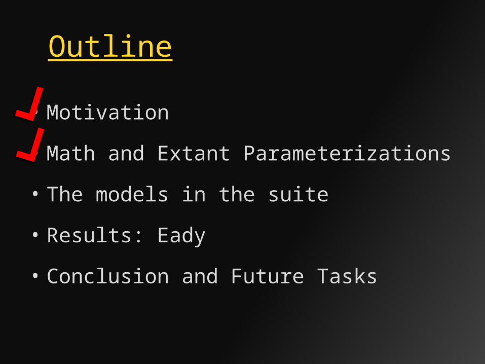
Outline
• Motivation
• Math and Extant Parameterizations
• The models in the suite
• Results: Eady
• Conclusion and Future Tasks

Figure courtesy of Baylor Fox-Kemper

The evolution of a Parameterization
1. Figure out that you need a parameterization (Bryan 1969)!
2. Discover your parameterization isn’t doing well… (Sarmiento 1982)
3. Improve theory: physical reasoning + mathematical form (Redi, 1982; Gent and McWilliams, 1990; Gent et al., 1995; Griffies, 1998)
4. Test the theory (Danabasoglu and McWilliams, 1995; Hirst and McDougall, 1996)
5. Validate against observations / improve theory

5. Validate against observations / improve theory
PROBLEM: What observations?
In real life, getting these observations is expensive, technically difficult, time-consuming, and you would need a LOT of them…
To complicate matters, it is not even clear how to apply observations to the values we use in a model (Marshall and Shuckburgh, 2006)…
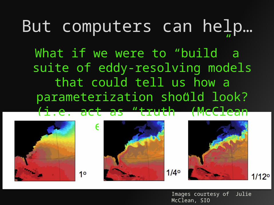
But computers can help…What if we were to “build” a suite of eddy-
resolving models that could tell us how a parameterization should look? (i.e. act as
“truth” (McClean et al., 2008)
Images courtesy of Julie McClean, SIO
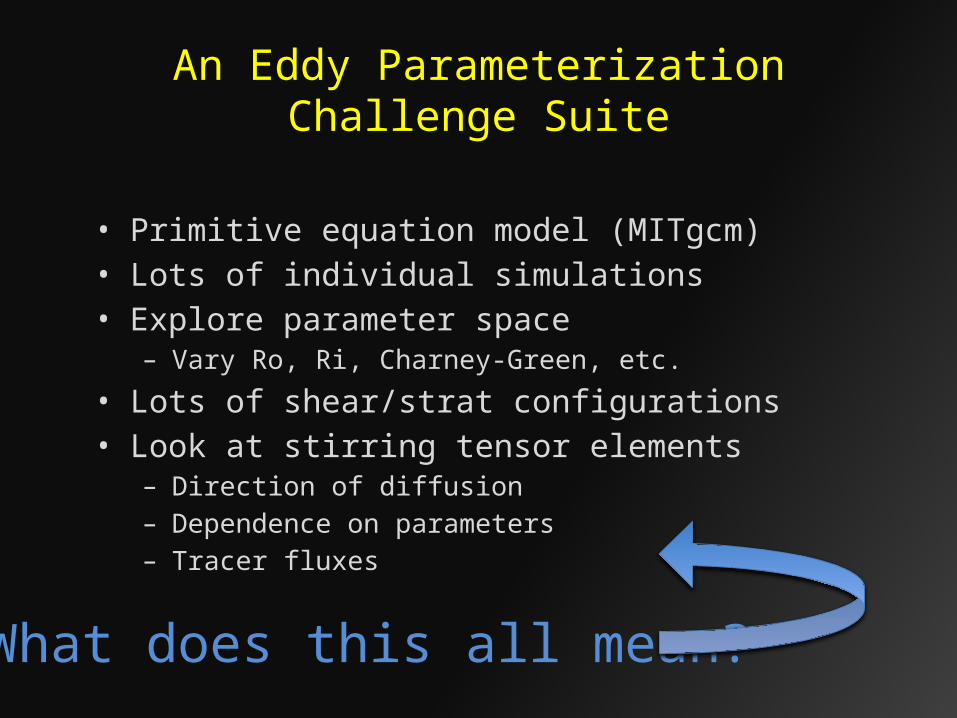
• Primitive equation model (MITgcm)• Lots of individual simulations• Explore parameter space
– Vary Ro, Ri, Charney-Green, etc.
• Lots of shear/strat configurations• Look at stirring tensor elements
– Direction of diffusion– Dependence on parameters– Tracer fluxes
What does this all mean?
An Eddy Parameterization Challenge Suite
Outline
• Motivation
• Math and Extant Parameterizations
• The models in the suite
• Results: Eady
• (Early) Results: Exponential
Outline

The Tracer Flux-Gradient Relationship
Relates the subgridscale eddy fluxes to coarse-grid gradient
Is the basis for most modern parameterization methods (GM90, Redi, etc.)
GOAL: We want R.

What do we know about the transport tensor R ?
• R varies in time and space
• R is 3 x 3 in three dimensions (2 x 2 in 2D)
• The structure of R should be deterministic
• Based on physics or the phenomenology of turbulence
• Not stochastic (…)
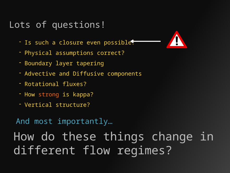
Lots of questions!
- Is such a closure even possible?
- Physical assumptions correct?
- Boundary layer tapering
- Advective and Diffusive components
- Rotational fluxes?
- How strong is kappa?
- Vertical structure?
And most importantly…
How do these things change in different flow regimes?
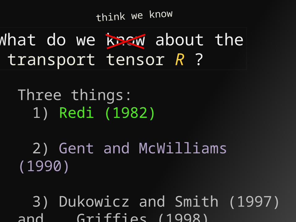
What do we know about the transport tensor R ?
think we know
Three things:1) Redi (1982)
2) Gent and McWilliams (1990)
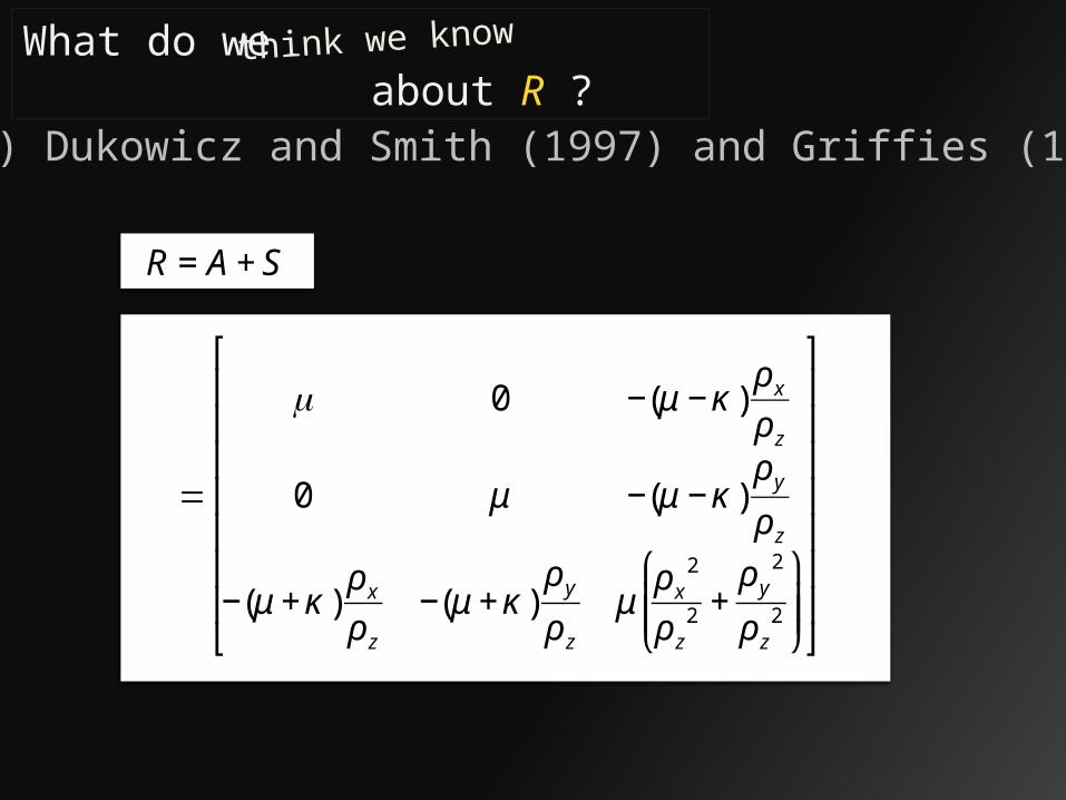
3) Dukowicz and Smith (1997) and Griffies (1998)
What do we about R ?think we know
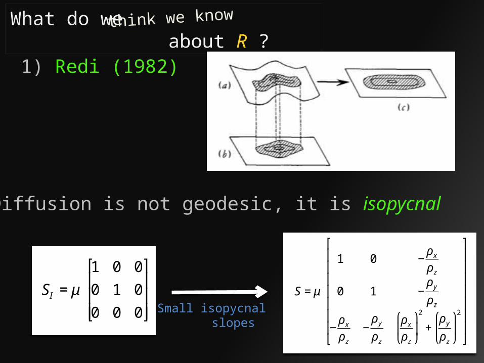
1) Redi (1982)
Diffusion is not geodesic, it is isopycnal
€
SI = μ
1 0 0
0 1 0
0 0 0
⎡
⎣
⎢ ⎢ ⎢
⎤
⎦
⎥ ⎥ ⎥
€
S = μ
1 0 −ρ xρ z
0 1 −ρ yρ z
−ρ xρ z
−ρ yρ z
ρ xρ z
⎛
⎝ ⎜
⎞
⎠ ⎟
2
+ρ yρ z
⎛
⎝ ⎜
⎞
⎠ ⎟
2
⎡
⎣
⎢ ⎢ ⎢ ⎢ ⎢ ⎢ ⎢
⎤
⎦
⎥ ⎥ ⎥ ⎥ ⎥ ⎥ ⎥
Small isopycnal slopes

What do we about R ?think we know
2) Gent and McWilliams (1990)
QUESTION: What happens if we diffuse density (i.e. use Redi) along an isopycnal?
ANSWER: Nothing!
Then Redi alone is inadequate… there must be another piece to this.
What do we about R ?think we know
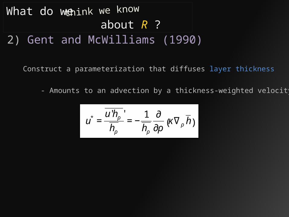
2) Gent and McWilliams (1990)
Construct a parameterization that diffuses layer thickness
- Amounts to an advection by a thickness-weighted velocity
€
u* =u'hρ '
hρ= −
1
hρ
∂
∂ρκ∇ρ h( )

What do we about R ?think we know
2) Gent and McWilliams (1990)
- Properties of
€
u*
- Nondivergent:
€
∇ ⋅ u* = 0
- No flow normal to boundaries:
€
u*⋅ n = 0 on ∂Ω
- Conserves all domain-averaged moments of density
- Conserves all domain-averaged tracer moments
- Skew flux (TEM):
€
u* ⋅ ∇ρ = 0
- Conserves tracer mean, reduces higher moments between isopycnal surfaces
What do we about R ?think we know
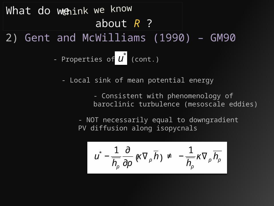
2) Gent and McWilliams (1990) – GM90
- Properties of
€
u*(cont.)
- Local sink of mean potential energy
- Consistent with phenomenology of baroclinic turbulence (mesoscale eddies)
€
u* −1
hρ
∂
∂ρκ∇ρ h( ) ≠ −
1
hρκ∇ρ hρ
- NOT necessarily equal to downgradient PV diffusion along isopycnals

What do we about R ?think we know
1) Redi (1982) – diffusion (mixing)
2) GM90 – advection (stirring)€
S = μ
1 0 −ρ xρ z
0 1 −ρ yρ z
−ρ xρ z
−ρ yρ z
ρ xρ z
⎛
⎝ ⎜
⎞
⎠ ⎟
2
+ρ yρ z
⎛
⎝ ⎜
⎞
⎠ ⎟
2
⎡
⎣
⎢ ⎢ ⎢ ⎢ ⎢ ⎢ ⎢
⎤
⎦
⎥ ⎥ ⎥ ⎥ ⎥ ⎥ ⎥
€
u* = −1
hρ
∂
∂ρκ∇ρ h( )
What do we about R ?think we know
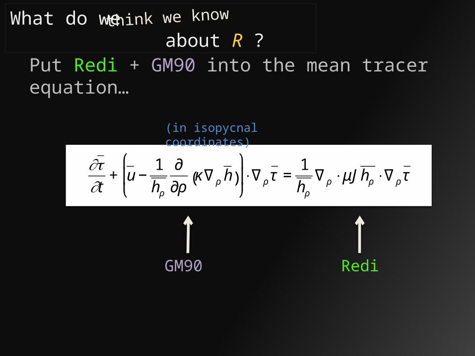
Put Redi + GM90 into the mean tracer equation…
€
∂τ∂t
+ u −1
hρ
∂
∂ρκ∇ρ h( )
⎛
⎝ ⎜
⎞
⎠ ⎟⋅∇ρ τ =
1
hρ∇ρ ⋅ μJhρ ⋅ ∇ρ τ
(in isopycnal coordinates)
GM90 Redi
What do we about R ?think we know
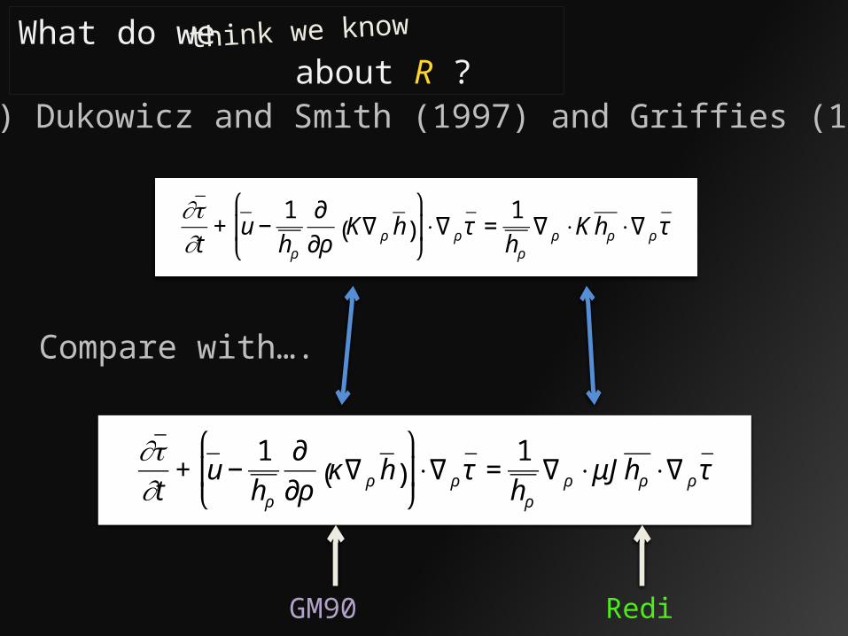
3) Dukowicz and Smith (1997) and Griffies (1998)
€
∂τ∂t
+ u −1
hρ
∂
∂ρK∇ρ h( )
⎛
⎝ ⎜
⎞
⎠ ⎟⋅∇ρ τ =
1
hρ∇ρ ⋅Khρ ⋅ ∇ρ τ
€
∂τ∂t
+ u −1
hρ
∂
∂ρκ∇ρ h( )
⎛
⎝ ⎜
⎞
⎠ ⎟⋅∇ρ τ =
1
hρ∇ρ ⋅ μJhρ ⋅ ∇ρ τ
Compare with….
GM90 Redi

What do we about R ?think we know
3) Dukowicz and Smith (1997) and Griffies (1998)
€
κ =μ
The thickness diffusivity coefficient is the same as the isopycnal diffusivity coefficient (?!)
What do we do with this information?
What do we about R ?think we know
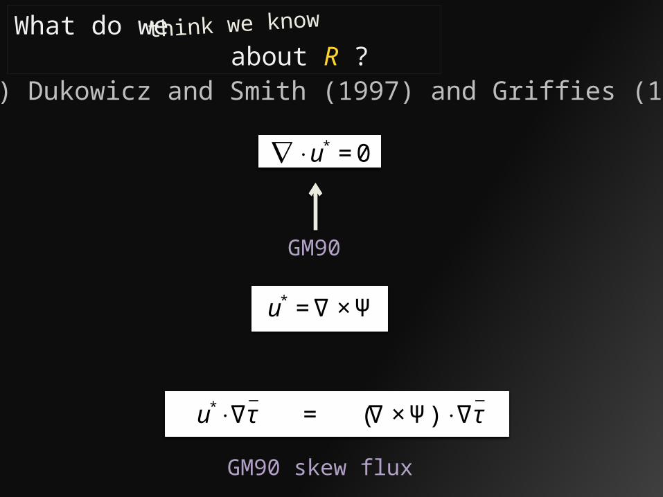
3) Dukowicz and Smith (1997) and Griffies (1998)
€
∇ ⋅ u* = 0
€
u* =∇ × Ψ
€
u*⋅ ∇τ = ∇ × Ψ( ) ⋅ ∇τ
GM90
GM90 skew flux
€
a × b( ) ⋅ c = a ⋅ (b × c)
Identity
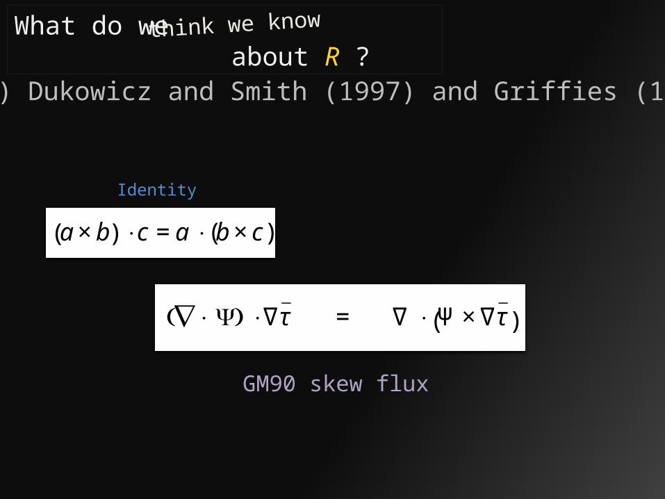
What do we about R ?think we know
3) Dukowicz and Smith (1997) and Griffies (1998)
€
∇×Ψ( ) ⋅ ∇τ = ∇ ⋅ Ψ ×∇τ( )
GM90 skew flux

€
a × b =
0 −a3 a2
a3 0 −a1
−a2 a1 0
⎡
⎣
⎢ ⎢ ⎢
⎤
⎦
⎥ ⎥ ⎥
b1
b2
b3
⎡
⎣
⎢ ⎢ ⎢
⎤
⎦
⎥ ⎥ ⎥
Identity
What do we about R ?think we know
3) Dukowicz and Smith (1997) and Griffies (1998)
€
∇×Ψ( )⋅∇τ = ∇⋅
0 −Ψ3 Ψ2
Ψ3 0 −Ψ1
−Ψ2 Ψ1 0
⎡
⎣
⎢ ⎢ ⎢
⎤
⎦
⎥ ⎥ ⎥
τ x
τ y
τ z
⎡
⎣
⎢ ⎢ ⎢
⎤
⎦
⎥ ⎥ ⎥
⎛
⎝
⎜ ⎜ ⎜
⎞
⎠
⎟ ⎟ ⎟ = ∇⋅ A∇τ
GM90 skew flux
What do we about R ?think we know
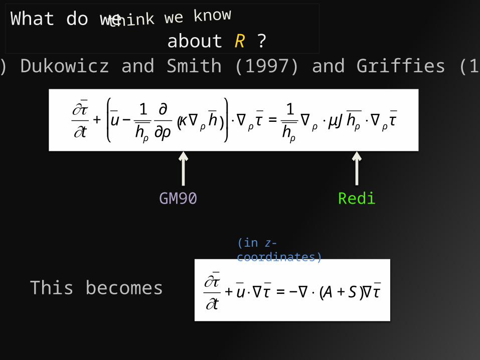
3) Dukowicz and Smith (1997) and Griffies (1998)
€
∂τ∂t
+ u −1
hρ
∂
∂ρκ∇ρ h( )
⎛
⎝ ⎜
⎞
⎠ ⎟⋅∇ρ τ =
1
hρ∇ρ ⋅ μJhρ ⋅ ∇ρ τ
GM90 Redi
€
∂τ∂t
+ u⋅ ∇τ = −∇⋅ A + S( )∇τ
(in z-coordinates)
This becomes
What do we about R ?think we know
3) Dukowicz and Smith (1997) and Griffies (1998)
€
R = A + S
€
=
μ 0 − μ − κ( )ρ xρ z
0 μ − μ − κ( )ρ yρ z
− μ + κ( )ρ xρ z
− μ + κ( )ρ yρ z
μρ x
2
ρ z2 +ρ y
2
ρ z2
⎛
⎝ ⎜ ⎜
⎞
⎠ ⎟ ⎟
⎡
⎣
⎢ ⎢ ⎢ ⎢ ⎢ ⎢ ⎢
⎤
⎦
⎥ ⎥ ⎥ ⎥ ⎥ ⎥ ⎥
What do we about R ?think we know
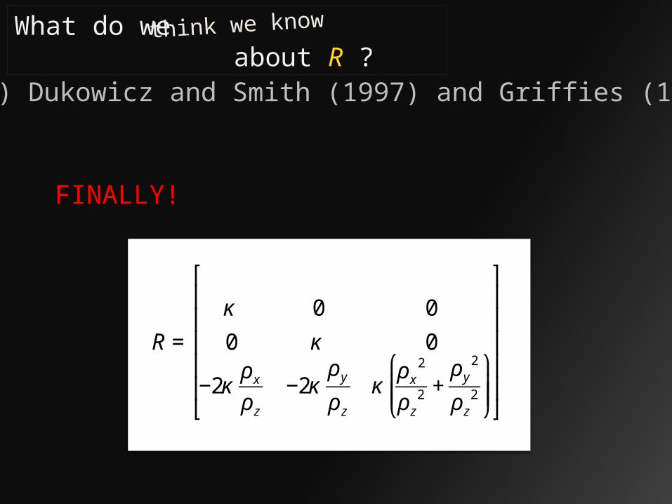
3) Dukowicz and Smith (1997) and Griffies (1998)
FINALLY!
€
R =
κ 0 0
0 κ 0
−2κρ xρ z
−2κρ yρ z
κρ x
2
ρ z2 +ρ y
2
ρ z2
⎛
⎝ ⎜ ⎜
⎞
⎠ ⎟ ⎟
⎡
⎣
⎢ ⎢ ⎢ ⎢ ⎢
⎤
⎦
⎥ ⎥ ⎥ ⎥ ⎥
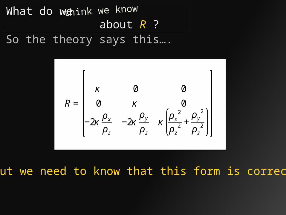
What do we about R ?think we know
€
R =
κ 0 0
0 κ 0
−2κρ xρ z
−2κρ yρ z
κρ x
2
ρ z2 +ρ y
2
ρ z2
⎛
⎝ ⎜ ⎜
⎞
⎠ ⎟ ⎟
⎡
⎣
⎢ ⎢ ⎢ ⎢ ⎢
⎤
⎦
⎥ ⎥ ⎥ ⎥ ⎥
So the theory says this….
But we need to know that this form is correct!
• Motivation
• Math and Extant Parameterizations
• The models in the suite
• Results: Eady
• Conclusion and Future Tasks
Outline

Mesoscale Characteristics
•50-100 km (ocean)
•Boundary Currents
•Eddies
•Ro = O(.01)
•Ri = O(1000)
•QG-scaling OK
The eddies extend the full depth of the water column, and are dominated by baroclinic instability.
Courtesy: K. Shafer Smith

We are going to look at properties of baroclinic instability alone.
Why?
Baroclinic instabilities dominate the mesoscale.
- Barotropic instabilities smaller than a deformation radius (too small).
- Symmetric instabilities appear at Richardson numbers < 0.95 (Nakamura, 1993).
- Kelvin-Helmholtz instabilities at Ri < 0.25.too low
http://www.coas.oregonstate.edu/research/po/research/chelton/index.html

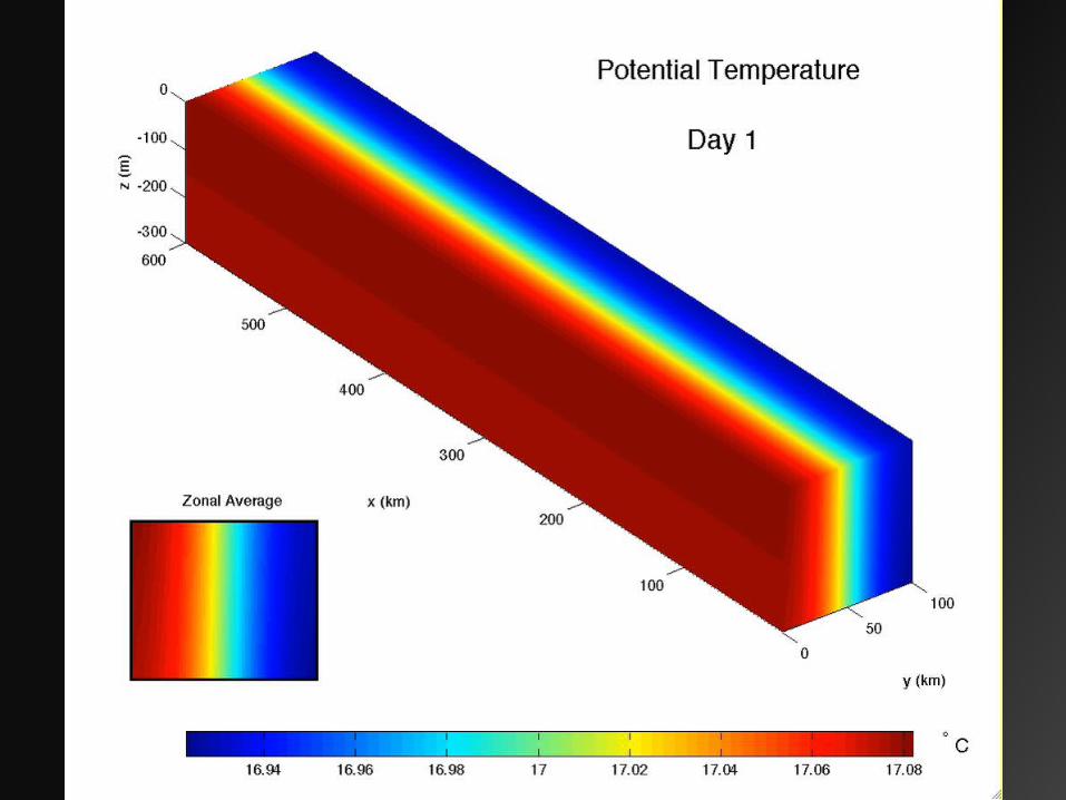
Construct models focusing only on baroclinic instability
Large Richardson number( anything >> 1 )
A front to make PE available for extraction
> deformation radius
= minimal barotropic component
900 x 150 x 60 grid

How do we solve for R ?
What happens if we have only one tracer?
Take a zonal average, and write the system out in full:
2 Equations…
Underdetermined! (not unique)
4 Unknowns!
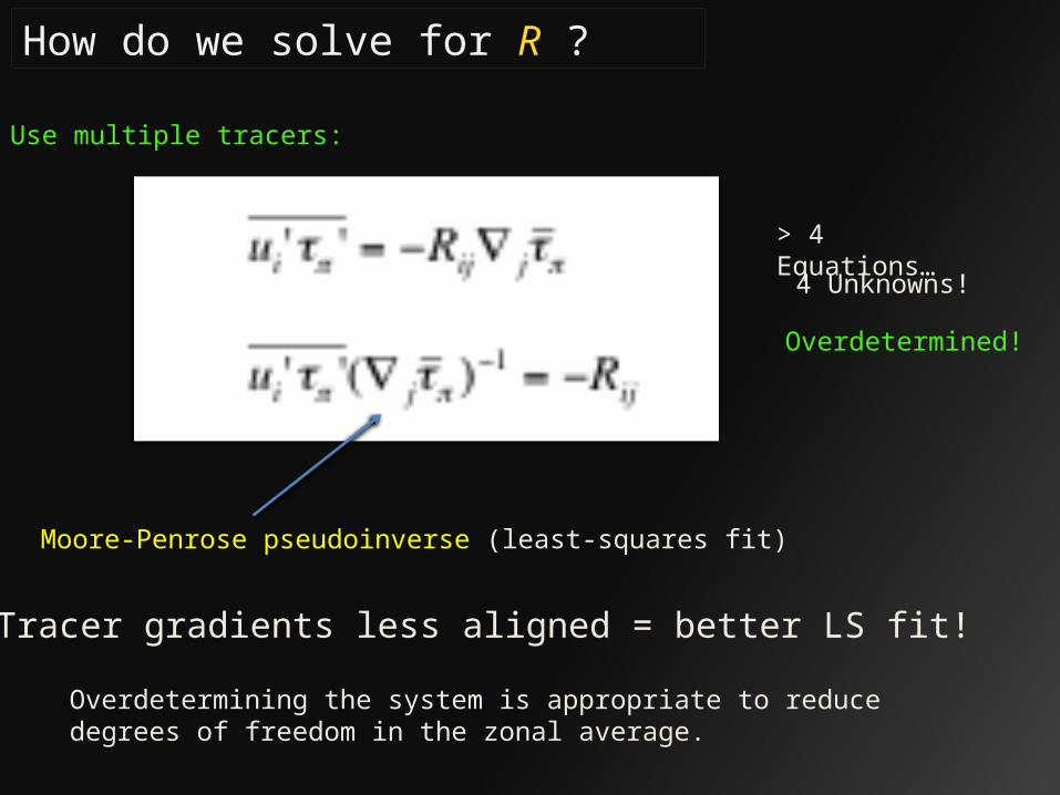
Use multiple tracers:
Tracer gradients less aligned = better LS fit!
Overdetermining the system is appropriate to reduce degrees of freedom in the zonal average.
How do we solve for R ?
4 Unknowns!
> 4 Equations…
Moore-Penrose pseudoinverse (least-squares fit)
Overdetermined!
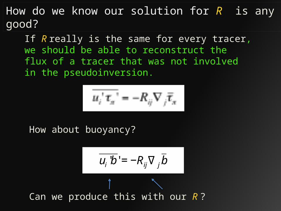
How do we know our solution for R is any good?
If R really is the same for every tracer, we should be able to reconstruct the flux of a tracer that was not involved in the pseudoinversion.
How about buoyancy?
€
ui 'b' = −Rij∇ jb
Can we produce this with our R ?
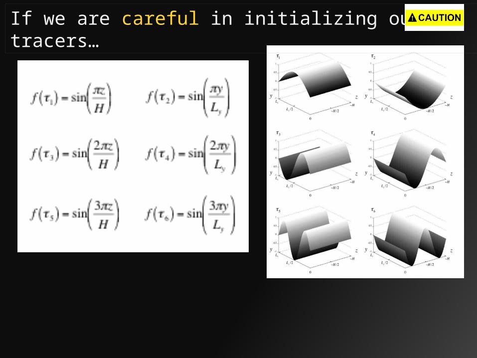
If we are careful in initializing our tracers…

Original fluxesReconstructed fluxes
Estimates of these buoyancy fluxes have improved substantially (error is now < 10%)… Used to be that getting error within a factor of two was the best we could do!
Good! (sinusoids) Bad! (not sinusoids)
The reconstruction is excellent.
Snapshot Snapshot
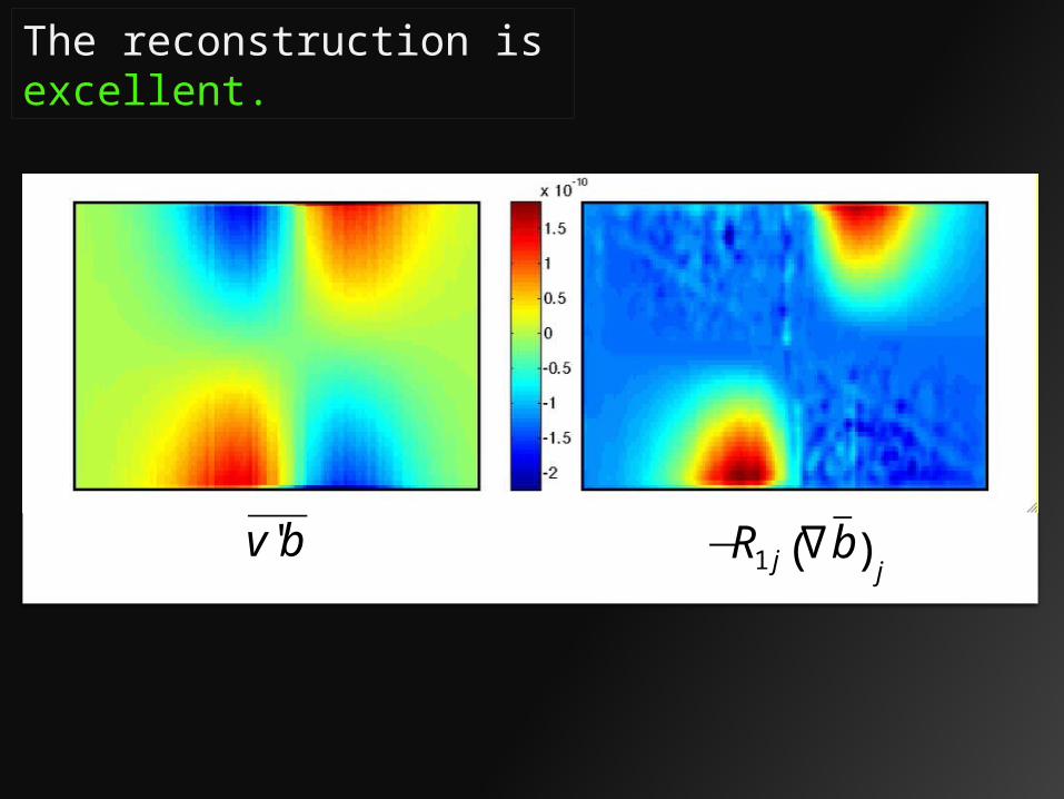
€
v'b'
€
−R1 j ∇b( )j
The reconstruction is excellent.

• Motivation
• Math and Extant Parameterizations
• The models in the suite
• Results: Eady
• Conclusion and Future Tasks
Outline

The Review before the Results
€
R =
κ 0 0
0 κ 0
−2κρ xρ z
−2κρ yρ z
κρ x
2
ρ z2 +ρ y
2
ρ z2
⎛
⎝ ⎜ ⎜
⎞
⎠ ⎟ ⎟
⎡
⎣
⎢ ⎢ ⎢ ⎢ ⎢
⎤
⎦
⎥ ⎥ ⎥ ⎥ ⎥
We think R looks like this:
So we are going to use a bunch of tracers that will tell us if we are right:
In 2D (zonal average)
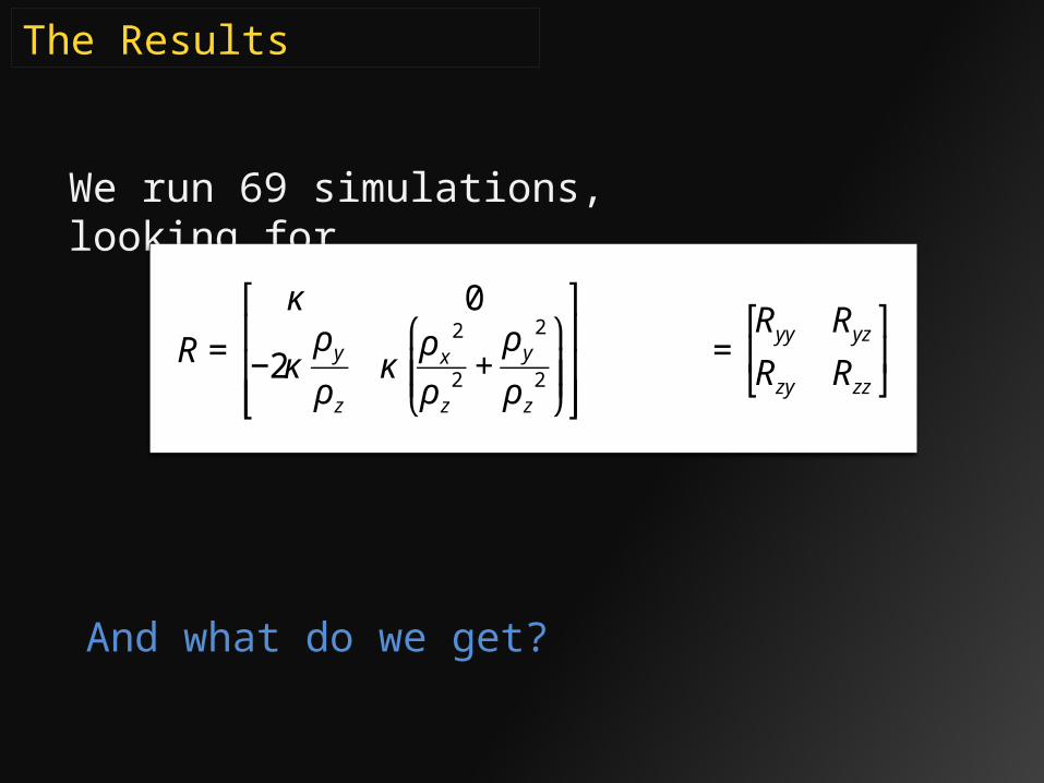
The Results
We run 69 simulations, looking for
€
R =
κ 0
−2κρ yρ z
κρ x
2
ρ z2 +ρ y
2
ρ z2
⎛
⎝ ⎜ ⎜
⎞
⎠ ⎟ ⎟
⎡
⎣
⎢ ⎢ ⎢
⎤
⎦
⎥ ⎥ ⎥ =
Ryy RyzRzy Rzz
⎡
⎣ ⎢
⎤
⎦ ⎥
And what do we get?
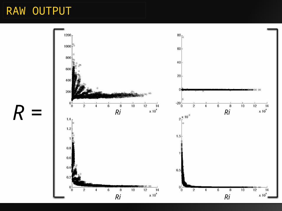
RAW OUTPUT
€
R =€
Ri
€
Ri
€
Ri
€
Ri
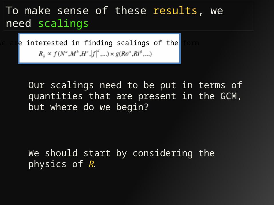
We are interested in finding scalings of the form
To make sense of these results, we need scalings
We should start by considering the physics of R.
Our scalings need to be put in terms of quantities that are present in the GCM, but where do we begin?

Previous Work (Fox-Kemper et al., 2008)
One could pursue naïve scalings based purely on dimensional analysis:
So that:
We find that this is inaccurate (see below).
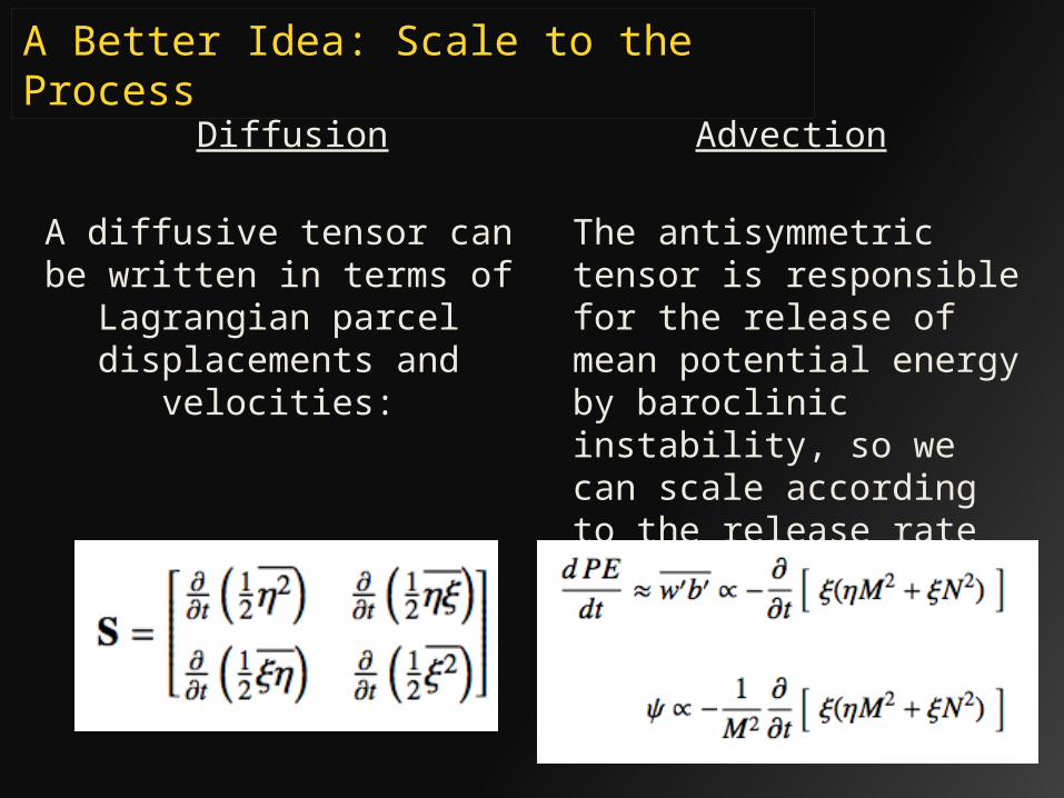
A Better Idea: Scale to the Process
Diffusion
A diffusive tensor can be written in terms of Lagrangian parcel displacements and
velocities:
Advection
The antisymmetric tensor is responsible for the release of mean potential energy by baroclinic instability, so we can scale according to the release rate

A Better Idea: Scale to the Process
Now choose length and time scales to substitute:
€
η∝N 2H
M 2
€
ξ ∝ H
€
∂η∂t
∝ v'2
€
∂ξ∂t∝ w'2
€
∝
N 2H
M 2 v '2H
M 2 v '2M 2 + w'2N 2 ⎛ ⎝ ⎜ ⎞
⎠ ⎟
H
M 2 v '2M 2 + w'2N 2 ⎛ ⎝ ⎜ ⎞
⎠ ⎟ H w'2
⎡
⎣
⎢ ⎢ ⎢
⎤
⎦
⎥ ⎥ ⎥
€
∝ H
M 2 v '2M 2 + w'2N 2 ⎛ ⎝ ⎜ ⎞
⎠ ⎟

A Better Idea: Scale to the Process
Then with Dukowicz and Smith (1997), a dimensional base scaling for R should be:
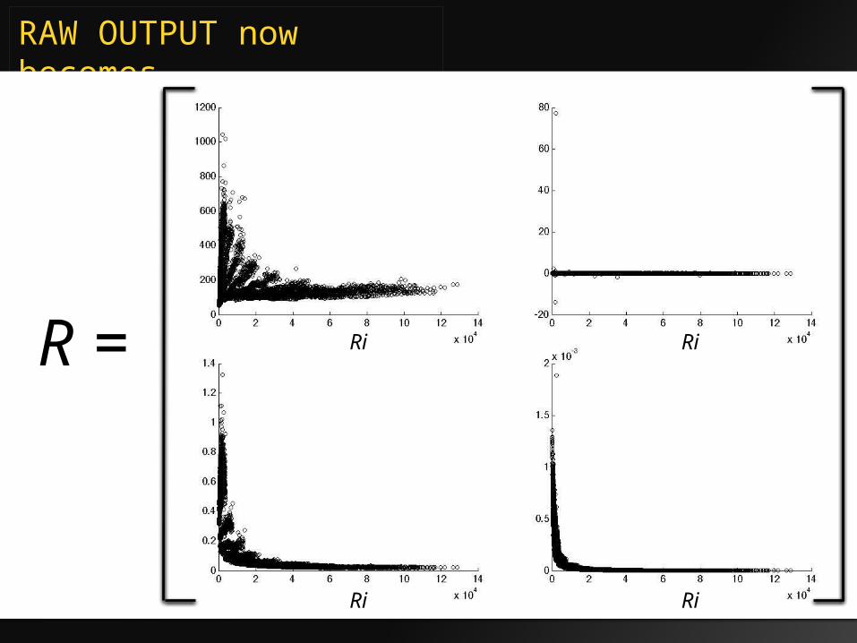
RAW OUTPUT now becomes…
€
R =€
Ri
€
Ri
€
Ri
€
Ri
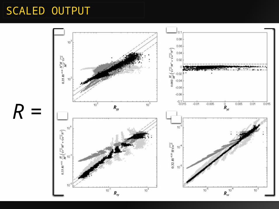
SCALED OUTPUT
€
R =€
Ryy
€
Ryz
€
Rzz
€
Rzy

SCALED OUTPUT
Our 69 simulations (~5000 data points) suggest scaling for R like so:
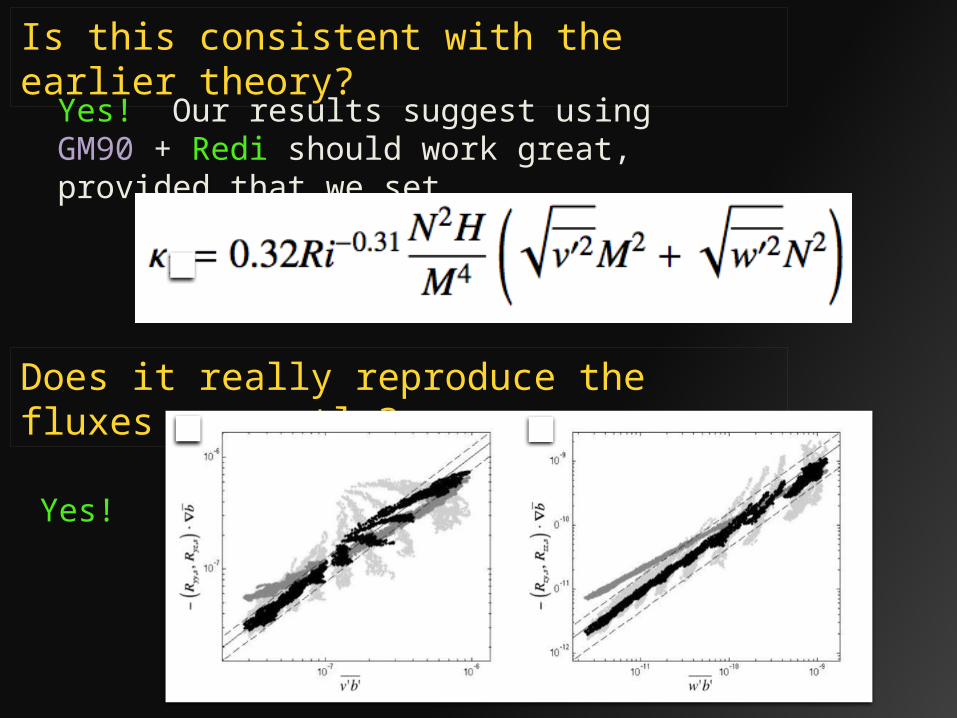
Is this consistent with the earlier theory?
Yes! Our results suggest using GM90 + Redi should work great, provided that we set
Does it really reproduce the fluxes correctly?
Yes!
• Motivation
• Math and Extant Parameterizations
• The models in the suite
• Results: Eady
• Conclusion and Future Tasks
Outline
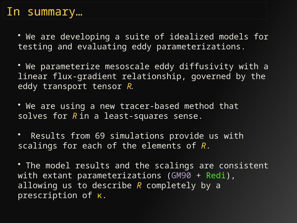
In summary…
• We are developing a suite of idealized models for testing and evaluating eddy parameterizations.
• We parameterize mesoscale eddy diffusivity with a linear flux-gradient relationship, governed by the eddy transport tensor R.
• We are using a new tracer-based method that solves for R in a least-squares sense.
• Results from 69 simulations provide us with scalings for each of the elements of R.
• The model results and the scalings are consistent with extant parameterizations (GM90 + Redi), allowing us to describe R completely by a prescription of κ.
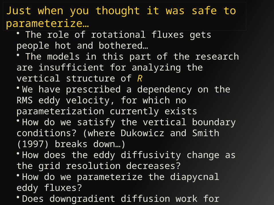
Just when you thought it was safe to parameterize…
• The role of rotational fluxes gets people hot and bothered…• The models in this part of the research are insufficient for analyzing the vertical structure of R• We have prescribed a dependency on the RMS eddy velocity, for which no parameterization currently exists• How do we satisfy the vertical boundary conditions? (where Dukowicz and Smith (1997) breaks down…)• How does the eddy diffusivity change as the grid resolution decreases?• How do we parameterize the diapycnal eddy fluxes?• Does downgradient diffusion work for potential vorticity? (more controversy)