Page 1
AN EFFICIENT LIBRARY FOR PARALLEL
RAY TRACING AND ANIMATION
by
JOHN EDWARD STONE, 1971–
A THESIS
Presented to the Faculty of the Graduate School of the
UNIVERSITY OF MISSOURI—ROLLA
In Partial Fulfillment of the Requirements for the Degree
MASTER OF SCIENCE IN COMPUTER SCIENCE
1998
Approved by
Fikret Ercal, Advisor Frank G. Walters
Hardy J. Pottinger
Page 2
c©1998
John Edward Stone
All Rights Reserved
Page 3
iii
ABSTRACT
A parallel ray tracing library is presented for rendering high detail images of
three dimensional geometry and computational fields. The library has been developed
for use on distributed memory and shared memory parallel computers and can also
run on sequential computers. Parallelism is achieved through the use of message
passing and threads. It is shown that the library achieves almost linear scalability
when run on large distributed memory parallel computers as well as large shared
memory parallel computers.
Several applications of parallel rendering are explored including rendering of
CAD models, animation, magnetic resonance imaging, and visualization of volumetric
flow fields. Ray tracing offers many advantages over polygon rendering techniques,
in its innate parallelism, and quality of output.
Page 4
iv
ACKNOWLEDGEMENTS
I would like to express my thanks to Dr. Fikret Ercal, my advisor, for his
patience, advice, and support throughout the course of my graduate level education.
I would also like to thank Frank G. Walters and Dr. Hardy J. Pottinger for being on
my committee, and for being excellent teachers.
I would like to thank Mark Underwood for his collaboration on the run-time
CFD visualization experiments included in this research. Special thanks go to Jeff
Bromberger for all of his help during the final stages of writing this thesis.
The support provided by the Computer Science Department of the University
of Missouri - Rolla through a half-time GRA appointment is gratefully acknowledged.
I would also like to acknowledge the computational resources provided by Oak Ridge
National Laboratory Center for Computational Sciences, the Hypersonic Vehicles Of-
fice at NASA Langley Research Center, NASA NAS, the Washington University of St.
Louis Computer and Communications Research Center, the University of Missouri-
Rolla Intelligent Systems Center, and the University of Missouri-Rolla Computer
Science Department.
Rolla, Missouri John Edward StoneApril, 1998
Page 5
v
TABLE OF CONTENTS
Page
ABSTRACT . . . . . . . . . . . . . . . . . . . . . . . . . . . . . . . . . . . . iii
ACKNOWLEDGEMENTS . . . . . . . . . . . . . . . . . . . . . . . . . . . . iv
LIST OF ILLUSTRATIONS . . . . . . . . . . . . . . . . . . . . . . . . . . . . viii
LIST OF TABLES . . . . . . . . . . . . . . . . . . . . . . . . . . . . . . . . . x
SECTION
I. INTRODUCTION . . . . . . . . . . . . . . . . . . . . . . . . . . . 1
II. CLASSICAL RAY TRACING . . . . . . . . . . . . . . . . . . . . . 4
A. BRIEF OVERVIEW OF THE RAY TRACING ALGORITHM 5
B. THE VIRTUAL CAMERA . . . . . . . . . . . . . . . . . . . . 5
C. VISIBLE SURFACE DETERMINATION . . . . . . . . . . . . 7
D. SURFACE SHADING . . . . . . . . . . . . . . . . . . . . . . . 8
1. Ambient Light . . . . . . . . . . . . . . . . . . . . . . . . . 8
2. Shadows . . . . . . . . . . . . . . . . . . . . . . . . . . . . . 9
3. Diffuse Shading . . . . . . . . . . . . . . . . . . . . . . . . . 11
4. Specular Highlights . . . . . . . . . . . . . . . . . . . . . . . 12
5. Specular Reflection . . . . . . . . . . . . . . . . . . . . . . . 12
6. Refraction . . . . . . . . . . . . . . . . . . . . . . . . . . . . 13
E. ALIASING . . . . . . . . . . . . . . . . . . . . . . . . . . . . . 15
F. NUMERICAL PRECISION AND RECURSION . . . . . . . . . 17
III. SURFACE TEXTURING . . . . . . . . . . . . . . . . . . . . . . . 18
A. GENERATING OBJECT SPACE COORDINATES . . . . . . . 18
B. COORDINATE TRANSFORMATION . . . . . . . . . . . . . . 18
C. TEXTURE LOOKUP . . . . . . . . . . . . . . . . . . . . . . . 19
D. IMPROVING MAPPING QUALITY . . . . . . . . . . . . . . . 20
Page 6
vi
E. IMAGE MAPPED TEXTURES . . . . . . . . . . . . . . . . . . 21
F. PROCEDURAL TEXTURING . . . . . . . . . . . . . . . . . . 22
IV. VOLUME RENDERING . . . . . . . . . . . . . . . . . . . . . . . . 24
A. VOLUME RENDERING TECHNIQUES . . . . . . . . . . . . . 25
B. VOLUME RENDERING USING RAY TRACING . . . . . . . 26
C. VOXEL INTEGRATION . . . . . . . . . . . . . . . . . . . . . 27
D. VOXEL SHADING . . . . . . . . . . . . . . . . . . . . . . . . . 28
E. VOLUME FILTERING AND ANTIALIASING . . . . . . . . . 29
V. RAY TRACING ACCELERATION TECHNIQUES . . . . . . . . . 30
A. BOUNDING HIERARCHIES AND SPATIAL SUBDIVISION . 31
B. SHADOW CACHING AND LIGHT BUFFERS . . . . . . . . . 32
VI. PARALLEL RAY TRACING . . . . . . . . . . . . . . . . . . . . . 37
A. DISTRIBUTED MEMORY RAY TRACING . . . . . . . . . . . 40
1. MPI . . . . . . . . . . . . . . . . . . . . . . . . . . . . . . . 42
2. Distributed Memory Adaptation of Ray Tracing Algorithms 43
3. Concurrent I/O . . . . . . . . . . . . . . . . . . . . . . . . . 45
4. Distributed Memory Scalability Results . . . . . . . . . . . . 46
B. MULTITHREADED RAY TRACING . . . . . . . . . . . . . . 48
1. Multithreaded Adaptation of Ray Tracing Algorithms . . . . 52
2. Asynchronous I/O . . . . . . . . . . . . . . . . . . . . . . . 53
3. Large Scene Scalability Results . . . . . . . . . . . . . . . . 54
C. HYBRID THREADS AND MESSAGE PASSING . . . . . . . . 58
1. Paragon XPS/15 . . . . . . . . . . . . . . . . . . . . . . . . 58
2. Hybrid Parallel Scalability Results . . . . . . . . . . . . . . 60
VII. RAY TRACING APPLICATIONS . . . . . . . . . . . . . . . . . . 63
A. ARCHITECTURE . . . . . . . . . . . . . . . . . . . . . . . . . 63
Page 7
vii
B. CAD/CAM . . . . . . . . . . . . . . . . . . . . . . . . . . . . . 64
C. MOLECULAR VISUALIZATION . . . . . . . . . . . . . . . . . 65
D. MEDICAL IMAGING . . . . . . . . . . . . . . . . . . . . . . . 66
E. FLOW FIELD VISUALIZATION . . . . . . . . . . . . . . . . . 67
F. STANDARD PROCEDURAL DATABASE IMAGES . . . . . . 69
VIII.CONCLUSIONS . . . . . . . . . . . . . . . . . . . . . . . . . . . . 71
A. FUTURE RESEARCH . . . . . . . . . . . . . . . . . . . . . . . 72
BIBLIOGRAPHY . . . . . . . . . . . . . . . . . . . . . . . . . . . . . . . . . 75
VITA . . . . . . . . . . . . . . . . . . . . . . . . . . . . . . . . . . . . . . . . 79
Page 8
viii
LIST OF ILLUSTRATIONS
Figure Page
1 Virtual Camera and Image Plane . . . . . . . . . . . . . . . . . . . . . . 6
2 Shadow Cast by an Object . . . . . . . . . . . . . . . . . . . . . . . . . . 10
3 Diffuse Illumination of an Object . . . . . . . . . . . . . . . . . . . . . . 11
4 Phong Highlighting . . . . . . . . . . . . . . . . . . . . . . . . . . . . . . 13
5 Specular Reflection . . . . . . . . . . . . . . . . . . . . . . . . . . . . . . 14
6 Refraction . . . . . . . . . . . . . . . . . . . . . . . . . . . . . . . . . . . 15
7 Block Cyclic Ray Tracing Decomposition . . . . . . . . . . . . . . . . . . 40
8 Scanline Cyclic Ray Tracing Decomposition . . . . . . . . . . . . . . . . 41
9 Pixel Cyclic Ray Tracing Decomposition . . . . . . . . . . . . . . . . . . 41
10 Plot of Execution Time for the SPD Balls Scene . . . . . . . . . . . . . . 47
11 Plot of Efficiency for the SPD Balls Scene . . . . . . . . . . . . . . . . . 47
12 Data Corruption in Unsynchronized Concurrent Memory Access . . . . . 51
13 Multithreaded Locking Strategies . . . . . . . . . . . . . . . . . . . . . . 52
14 Efficiency of Asynchronous I/O versus Synchronous I/O . . . . . . . . . . 55
15 Large Scene Scalability Results . . . . . . . . . . . . . . . . . . . . . . . 57
16 Hybrid Ray Tracing Decomposition . . . . . . . . . . . . . . . . . . . . . 59
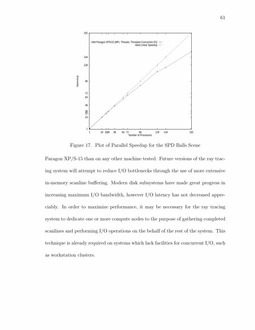
17 Plot of Parallel Speedup for the SPD Balls Scene . . . . . . . . . . . . . 61
18 Plot of Parallel Efficiency for the SPD Balls Scene . . . . . . . . . . . . . 62
19 Conference Room . . . . . . . . . . . . . . . . . . . . . . . . . . . . . . . 63
20 X-Wing Model . . . . . . . . . . . . . . . . . . . . . . . . . . . . . . . . 64
21 Molecular Visualization . . . . . . . . . . . . . . . . . . . . . . . . . . . . 65
22 Volume Rendered MRI Scan . . . . . . . . . . . . . . . . . . . . . . . . . 66
23 Conceptual Schematic of an Injector Flow Field . . . . . . . . . . . . . . 67
24 Volume Rendered Injector Flow Field . . . . . . . . . . . . . . . . . . . . 68
Page 9
ix
25 SPD Teapot . . . . . . . . . . . . . . . . . . . . . . . . . . . . . . . . . . 69
26 SPD “Sphereflake” . . . . . . . . . . . . . . . . . . . . . . . . . . . . . . 70
Page 10
x
LIST OF TABLES
Table Page
I Efficiency of Asynchronous I/O versus Blocking I/O . . . . . . . . . . . 54
Page 11
I. INTRODUCTION
The need for high quality rendering of three dimensional geometry and vector
fields has grown tremendously in recent years. As a result, much work has been done
in the design of algorithms and systems to render photorealistic images of these objects
on computers. Many of the algorithms used to generate high quality three dimensional
images require a lot of processing time to execute. To date, many researchers have
created high efficiency graphics algorithms on sequential computers. Through this
research, modern graphics algorithms now achieve peak efficiency and performance
on sequential computers in use today. Although many algorithms currently in use are
already highly tuned, it is possible to further reduce execution time through the use of
many processors in parallel. By parallelizing the rendering process, execution time can
be reduced by more than two orders of magnitude, given appropriate computational
resources.
In this thesis a parallel ray tracing library is presented for use on a wide range
of parallel computer systems. Ray tracing is one of many techniques for rendering
three dimensional images. Ray tracing is a rendering model which is based on the
physics of light and how it interacts with different materials. Ray tracing gets its name
from the use of simulated rays of light in producing images. In ray tracing, visible
surface determination, reflection, refraction, and shading are done using physically
based approximations of the way real light behaves. Ray tracing is capable of ren-
dering complex mathematical surfaces, multi-dimensional vector fields, and discrete
Page 12
2
polygonal meshes. Classical sequential ray tracing algorithms can be adapted for par-
allel execution environments, and are well suited for the production of photorealistic
images. Other rendering techniques which are computationally cheaper are typically
limited to the use of polygonal meshes for modeling objects, and can be much more
difficult to parallelize efficiently. Ray tracing is well suited to parallel computation.
One of the most difficult parts of writing a library for use on parallel computers
are the choices of what operating systems interfaces or extensions to use when writing
the library. Inclusion of a platform-specific extension or feature often limits the
portability of the library to other platforms, and makes maintenance of the library
difficult. In order for the library to automatically take advantage of parallelism,
two key programming paradigms are exploited; inter-processor message passing, and
multithreading. Message passing is used on distributed memory parallel computers
for process synchronization, communication, and disk I/O. Message passing has been
a very successful technique in implementing parallel applications on a wide range
of computing platforms which range from clusters of workstations all the way to
massively parallel distributed memory supercomputers. In order to achieve portability
to a wide range of computers, the ray tracing library encapsulates system specific
message passing routines within its own internal message handling routines. This
allows the library to be ported to new message passing systems and architectures by
modifying a small group of message passing abstraction routines.
Threads are a natural and efficient way to schedule work on multiprocessor sys-
tems, currently they may only be used on shared memory multiprocessor computers.
Page 13
3
Recent advances in distributed shared memory research may make threads applicable
to distributed memory machines in the future. As with the message passing routines,
the ray tracing library encapsulates system specific thread routines within internal
abstraction routines to make porting an easier task.
During the design and implementation of the ray tracing library it was neces-
sary to limit the scope of the work to something which could be accomplished in a
reasonable amount of time by a single researcher. To this end, the work presented
in this thesis is focused on real-world applicability, performance, and portability.
Since ray tracing is a subject which has been researched by many others before, a
great many algorithms already exist for the efficient implementation of ray tracing
on sequential computers. Most ray tracing algorithms designed for use on sequen-
tial computers may be used as-is in a parallel environment, provided that care is
taken in their implementation. During the course of the design of the ray tracing
library, standard algorithms were used when possible. In cases where this was not
possible, standard sequential algorithms were adapted for use in a parallel execution
environment. Fortunately, ray tracing affords a great degree of parallelism and can
be implemented in parallel with relatively few restrictions or complications.
Page 14
4
II. CLASSICAL RAY TRACING
Ray tracing as a technique for rendering three dimensional images was first
introduced by Appel in 1968 [1]. Appel introduced ray tracing of objects, including
surface shading and shadows. Goldstein and Nagel also developed ray tracing, but
their original work dealt with simulation of trajectories of ballistic projectiles and
nuclear particles. Goldstein and Nagel later introduced the use of binary set op-
erations to implement constructive solid geometry in ray tracing [14]. Research by
Whitted [54], and Kay [27] extended the ray tracing algorithm to handle specular
reflection and refraction. Among rendering techniques, ray tracing is best known
for its elegant solutions to shadow determination, specular reflection, refraction, and
volume rendering.
In any of the graphics rendering techniques used today, there are two main
tasks involved in generating an image; visible surface determination, and shading.
Visible surface determination is the process by which a renderer determines what ob-
jects or surfaces can be seen from a particular viewpoint. Shading is the process that
assigns a color to a point on or in an object. The color assignment is based on light-
ing, shadows, transparency, reflectivity, refractive index, and surface texture. Classic
ray tracing algorithms provide solutions for all of the local illumination properties
mentioned above, and can be further extended to handle global diffuse illumination.
Page 15
5
A. BRIEF OVERVIEW OF THE RAY TRACING ALGORITHM
Ray tracing attempts to model a subset of the real physical processes involved
in optics and lighting. The standard ray tracing algorithm relies on numerical ap-
proximations of physical behavior in order to achieve realistic shading with finite
computational resources. In real life, light emanates from a source in the form of
photons. The photons exit the light source and (ignoring relativistic and gravita-
tional lensing effects) travel in a straight line (a ray) until they encounter a surface
which interferes with further travel. The physical interaction between photons and
surface materials determine how they are absorbed, reflected, and transmitted. The
images we see with our own eyes are the result of billions of photons bouncing around,
some of which are absorbed by the retina in our eyes. This model is called forward
ray tracing. One could certainly implement this model on a computer, but there is a
major problem with the use of forward ray tracing, it would spend a large percentage
of its time simulating light that is never seen. Rather than spawning rays from light
sources to the eye, as it is in real life, it is more computationally efficient to trace rays
from the eye to the light sources. Backward ray tracing only performs calculations for
photons that are likely to be visible. An excellent introductory book on the subject
of ray tracing is “An Introduction to Ray Tracing”, by Glassner et al. [9].
B. THE VIRTUAL CAMERA
The first stage in the ray tracing algorithm is the generation of primary rays,
the rays which start the recursive ray tracing process. The camera model employed
by most ray tracing systems generates primary rays by simulating a simple pinhole
Page 16
6
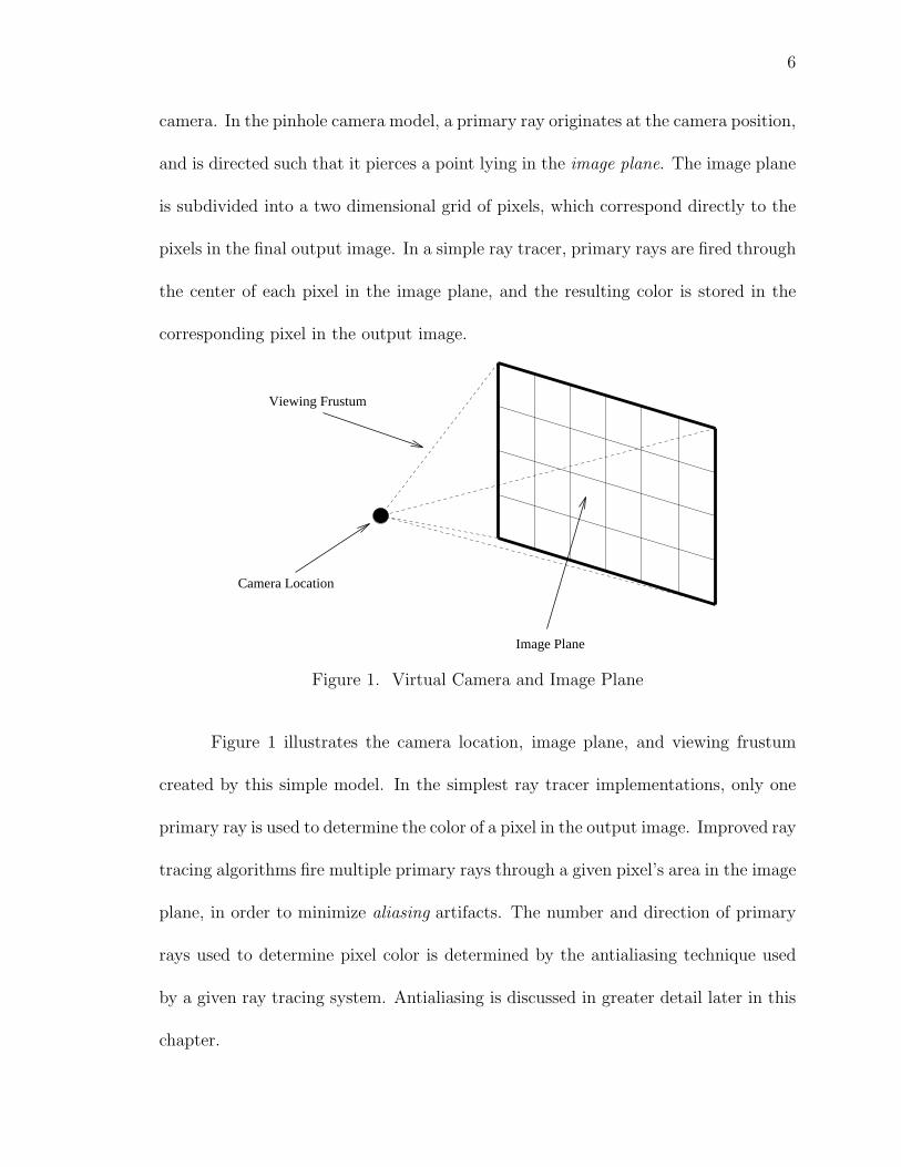
camera. In the pinhole camera model, a primary ray originates at the camera position,
and is directed such that it pierces a point lying in the image plane. The image plane
is subdivided into a two dimensional grid of pixels, which correspond directly to the
pixels in the final output image. In a simple ray tracer, primary rays are fired through
the center of each pixel in the image plane, and the resulting color is stored in the
corresponding pixel in the output image.
Camera Location
Image Plane
Viewing Frustum
Figure 1. Virtual Camera and Image Plane
Figure 1 illustrates the camera location, image plane, and viewing frustum
created by this simple model. In the simplest ray tracer implementations, only one
primary ray is used to determine the color of a pixel in the output image. Improved ray
tracing algorithms fire multiple primary rays through a given pixel’s area in the image
plane, in order to minimize aliasing artifacts. The number and direction of primary
rays used to determine pixel color is determined by the antialiasing technique used
by a given ray tracing system. Antialiasing is discussed in greater detail later in this
chapter.
Page 17
7
C. VISIBLE SURFACE DETERMINATION
Ray tracing differs from most other rendering techniques in the way it per-
forms visible surface determination. Polygon oriented rendering techniques represent
objects as collections of triangles or other planar polygons. In order to render curved
geometry with adequate precision, polygon renderers tessellate curved surfaces with
thousands of polygons. A significant problem with this approach is that no matter
how finely a surface is tessellated it is always possible to choose a viewing configura-
tion such that the edges of polygons can be seen. The only way to avoid this problem
in a polygonal representation is to tessellate curves so that constituent polygons are
smaller than a pixel in the resulting view. Many polygon based rendering systems
employ dynamic level of detail algorithms which adaptively tessellate surfaces based
on the viewing configuration.
Ray tracing performs visible surface determination separately for each pixel
in the rendered image. Camera rays are intersected with objects in the scene. The
intersection closest to the camera is taken as the visible surface. Since visible surface
determination is done with at least pixel level resolution, curved surfaces are accu-
rately sampled. Any kind of geometry that can be sampled via intersection tests can
be represented in a ray tracing system. In order to render a sphere in a polygon
based renderer, the sphere must be tessellated with polygons up to the required level
of detail. A ray tracer tests a ray for intersection with the sphere. If an intersection
exists, then the point or points at which the ray intersects the sphere are inserted
into an intersection list. Since intersection tests are performed for separately for each
Page 18
8
pixel, the surface of the sphere is sampled pixel accurate resolution, yielding a curved
looking surface regardless of the viewing configuration. The ray tracing process auto-
matically produces the highest level of detail, since it samples geometric structure at
each pixel. The results obtained by ray tracing are equivalent to tessellating a surface
down to sub-pixel sized polygons. The geometric representation used in ray tracing
can be much more memory efficient than that of a polygon renderer for this reason.
D. SURFACE SHADING
Once surface visibility has been determined through intersection tests with
the objects in a scene, a color must be assigned to the resulting surface at the closest
point of intersection. Surface shading can be done many different ways. Ray tracing
offers an elegant framework for performing a variety of shading operations. As with
visible surface determination, ray tracing performs shading calculations for each pixel
independently. Depending on the characteristics of an object’s material, factors such
as ambient light, diffuse light, reflection, refraction, and surface texture affect its
coloring. The per-pixel evaluation of lighting and texturing employed in ray tracing
allows stunningly realistic images to be produced.
1. Ambient Light. Although ray tracing systems are capable of realistically
emulating many optical effects, they typically employ simple algorithms for rendering
shadows and indirect illumination. The standard ray tracing model only accounts for
direct illumination; lighting attributed to rays which travel from a light source directly
to a surface, with no contributions from secondary reflections or transmissions from
other objects. In the real world, light emanates from a source, possibly reflecting off
Page 19
9
of many surfaces before illuminating a surface. A good example of indirect lighting
is a room with white walls, a table, and a lamp sitting on top of the table. In the
real world, light emanates from the lamp on the table, and bounces around the room
until it is completely absorbed by the surfaces in the room. Since the light is on the
table, there is a region of shadow underneath the table. The table blocks all direct
illumination from the lamp to the area underneath the table, leaving it in shadow.
In the real world, the shadow cast by the table is not absolutely dark. Secondary
reflections from the walls of the room illuminate the area underneath the table. The
ray tracing algorithm accounts for direct illumination caused by the lamp on the table,
but does not take into account the contributions of indirect lighting. Although the
area under the table is not in complete shadow in real life, a ray traced image of this
scene would yield an absolutely dark shadow under the table. A crude approximation
of the effects indirect lighting may be obtained through the use of a constant ambient
lighting value. For higher quality rendering, global illumination techniques such as
radiosity may be employed as a pre-processing step to ray tracing, providing more
realistic emulation of indirect lighting effects.
2. Shadows. The ray tracing algorithm handles shadows by spawning shadow
test rays from the intersection point on a surface towards each of the lights in the
scene. If a shadow ray encounters an object before it reaches the light, then the
point is in the shadow of the occluding object. In a simple implementation, only one
shadow ray is fired for each light, and the transparency of an object is not taken
into consideration. Improved shadow determination methods spawn multiple shadow
Page 20
10
rays towards each light, in order to soften the edges of a shadow, and reduce aliasing
artifacts. More sophisticated ray tracers may test an occluding object’s transparency,
index of refraction, and color in order to simulate filtering effects and caustics. Fig-
ure 2 illustrates a simple scene with an object casting a shadow onto a plane.
Light Source
Object Casting a Shadow
Shadow from Object
Camera
Primary Ray Shadow Test Ray
Figure 2. Shadow Cast by an Object
Shadow determination can be one of the most time consuming stages in the
ray tracing algorithm, since a shadow ray is spawned for every light source in the
scene, at every point where shading is performed. A simple optimization for shadow
testing is to provide an early exit in the intersection test code so that the shadow test
terminates immediately when any intersection is found between the light source and
the surface being shaded. This optimization works for ray tracers that do not handle
complex filtering and caustic effects. Two other optimization techniques which can
Page 21
11
greatly improve the efficiency of shadow testing are the shadow cache and the light
buffer algorithm [9].
3. Diffuse Shading. After shadow tests have determined that there are no
occlusions blocking a light source, surface shading calculations for that light may
begin. Diffuse shading determines the amount of light reflected from a dull matte
surface such as typing paper. A simple method for approximating the diffuse reflection
from a surface is to evaluate the cosine of the angle between the surface normal,
and a vector pointing in the direction of the light. This can easily be evaluated by
computing the dot product between the surface normal and the light vector, assuming
both vectors have already been normalized. The resulting scalar value represents the
diffuse contribution of the light source at that point on the surface. Figure 3 illustrates
the vectors used in the diffuse shading calculations.
Light Source
AngleRay Light Vector
SurfaceNormal
Camera
Object being shaded
Figure 3. Diffuse Illumination of an Object
Page 22
12
4. Specular Highlights. Specular highlights simulate the reflective character-
istics of shiny materials such as plastic and metal. These highlights are different from
perfect specular reflection such as a mirror. Specular highlights are used to model
imperfect reflecting surfaces. Rather than reflecting light only at one exact angle, im-
perfect surfaces reflect light over a range of angles. Smooth reflecting surfaces have a
very narrow range of angles for which reflectance is high. Rough surfaces have a high
reflectance over a wider range of angles. Romney [40] and Phong [36] [37] each devel-
oped shading equations for approximating specular reflections using a cosine function
raised to an exponent. This technique provides a computationally inexpensive alter-
native to calculating specular reflections by firing reflection rays. The drawback to
this technique is that it doesn’t take into account reflections of anything other than
the lights in a scene. For mirror reflections or more accurate specular reflections,
techniques that are more computationally expensive must be used. Figure 4 illus-
trates the geometry involved in performing shading for specular highlights based on
the cosine exponent model.
5. Specular Reflection. A ray tracer can simulate specular reflections for
surfaces which have mirror-like properties very easily, by spawning reflection rays
and adding the resulting color intensities to the intensities calculated for other surface
properties. For perfect reflectors such as a mirror, the distribution of reflection rays
lies entirely along a single ray. For reflectors which are imperfect, hazy, or blurred,
the distribution of reflection rays lies over a range of angles, which are narrower with
nearly perfect reflectors, and wider for hazy or blurred reflectors. Figure 5 illustrates
Page 23
13
Surface Normal
Reflection Ray
RayLight Source
Camera
Light Vector
Angle
Figure 4. Phong Highlighting
incident rays bouncing off of a planar mirror, hitting another object.
6. Refraction. All of the shading techniques discussed up to this point have
dealt with opaque surface characteristics. Transparent objects may allow transmis-
sion of light through the volume of the object depending on the index of refraction for
the object’s material and the index of refraction of surrounding space. In a simple im-
plementation, refractive effects are ignored, and a transmission ray continues through
the material along the same path as it enters and leaves an object. Refractive effects
can be calculated using Snell’s law. Figure 6 illustrates refraction at the interface
between two transparent materials with different indices of refraction.
A significant difficulty in implementing refractive effects properly lies in the
task of keeping track of the indices of refraction for the space a ray is entering or
leaving at any given time. When a new ray is created, it starts in some material.
As the ray continues through space, it enters and leaves other materials which may
Page 24
14
Surface Normal
Mirrored Plane
Angle ofIncidence
ReflectedAngle
Camera
Light Source
Ray
Reflection Ray
Light Vector
Object seen in reflection
Figure 5. Specular Reflection
have different indices of refraction. For ray tracing systems that only implement
solid geometric primitives, the task is straightforward. Indices of refraction can be
determined by the solids the ray is entering and leaving. For ray tracing systems which
allow the use of polygonal meshes for the representation of solids, keeping track of
the correct indices of refraction can be difficult. In these systems, some other method
must be employed to help the ray tracer “remember” what indices of refraction to
use on the two sides of the interface between the materials. One possible solution to
this problem is the use of a stack to keep track of the index of refraction for the space
the ray is leaving and entering at each interface. When the ray passes into an object,
the index of refraction for that object is pushed onto the top of the stack. When the
ray leaves the object, the index of refraction is popped off of the stack.
Page 25
15
Incident Ray Reflected Ray
Transmitted Ray
Material 2
Material 1
Surface Normal
Material Surface Interface
Angle
Angle
Figure 6. Refraction
E. ALIASING
Ray tracing is based on discrete sampling of a continuous sample space. Image
quality obtained by ray tracing is the direct result of the quality and representative-
ness of the samples taken. In order to achieve the highest image quality, antialiasing
techniques may greatly improve image quality with some additional computational
cost. Antialiasing algorithms typically cause multiple camera rays to be fired for
each output pixel. The number of extra rays and their directions are determined by
the antialiasing algorithm. Since aliasing can occur both spatially and temporally,
advanced ray tracers used for animation may distribute rays temporally as well as
spatially.
A variety of approaches to antialiasing may be used. Supersampling is a very
simple antialiasing technique which subdivides each pixel into smaller subpixels along
Page 26
16
a uniform grid. Camera rays are then fired for each of these subpixels, and the result-
ing colors are combined using simple averaging, or a weighted average, to produce the
resulting pixel. Although easy to implement, supersampling is still quite susceptible
to aliasing effects, and can be computationally wasteful when overused. A slight mod-
ification to the supersampling technique can make it more computationally efficient,
and give it greater flexibility. Adaptive supersampling attempts to determine areas
where aliasing effects occur, and automatically subdivides a pixel into subpixels, and
potentially recursively subdividing into even smaller subpixels based on differences
between adjacent pixels or subpixels. Adaptive supersampling techniques generally
employ simple metrics which measure the variance between the colors of neighboring
pixels. If neighboring pixels differ by more than a certain threshold, they are recur-
sively supersampled until either they differ by less than the threshold, or a maximum
cutoff subdivision depth has been reached. The resulting pixels are then averaged or
filtered to produce the final pixel color stored in the resulting image.
Adaptive supersampling based on a uniform grid subdivision scheme can still
suffer from grid alignment aliasing, even when supersampled to great depth. In
order to combat this problem, samples may be taken in a non-grid-aligned fashion.
The sample points may be determined pseudo-randomly for stochastic sampling, or
they may be chosen based on a statistical distribution. These techniques avoid grid
alignment aliasing artifacts and may require fewer samples to produce results of equal
quality to those obtained by grid-aligned sampling techniques of greater depth.
Page 27
17
F. NUMERICAL PRECISION AND RECURSION
The ray tracing algorithm can encounter problems when rendering some scenes
due to the finite precision of floating point arithmetic on computers. This problem
can manifest itself in the generation of rays for reflection, refraction, and shadows.
The problem occurs when a new ray is generated at a hit point on an object, going in
some new direction. In some cases a ray will tend to intersect the same surface it is
supposed to be leaving. In order to avoid this problem, a ray tracer can manipulate
the ray’s starting point so that it is far enough off of the surface it is leaving that the
intersection testing routines do not erroneously intersect with the surface the ray is
leaving.
Another problem that can occur is the generation of an infinite, or nearly in-
finite number of reflection or transmission rays. In a scene containing two perfectly
parallel, perfectly reflective mirrors, it is possible for a ray which is perfectly per-
pendicular to endlessly generate reflection rays. In the case of transmission, a ray
may encounter total internal reflection, inside of an appropriately curved object such
that it also endlessly generates transmission rays. One way to prevent a ray tracer
from getting stuck in such pathological cases is to set a hard limit on the maximum
level of recursion for the rays in a scene. A recursion limit of one would only allow
primary rays to be traced. Recursion levels greater than one would allow reflections
and transmissions to be ray traced. When the maximum level of recursion is reached,
rather than generating reflection or transmission rays, the scene background color is
used [9].
Page 28
18
III. SURFACE TEXTURING
A. GENERATING OBJECT SPACE COORDINATES
Before implementing a transformation procedure that maps 3-D object space
coordinates to parametric coordinates, a ray tracer needs to generate the object space
coordinates to be mapped. In ray tracing, this is easily done by using the point
where a ray intersects the surface of the object to be texture mapped. The added
cost of texture mapping is negligible compared to the cost of intersection testing, so
texture maps are a computationally cheap alternative to high geometric complexity.
Texture maps can provide levels of detail which are impractical to represent with
highly tessellated surfaces of constant textures. Techniques such as MIP mapping [55]
provide effective ways to avoid aliasing artifacts, as well as providing some depth of
field effect with minimal additional computational cost.
B. COORDINATE TRANSFORMATION
In order to implement texture mapping in a ray tracer, the first step is to
create a mapping function which takes a 3-D coordinate as its input, and generates a
2-D parametric texture coordinate as its output. These transformations provide the
mechanism for mapping a two dimensional image or procedural texture, onto a three
dimensional surface. An easy coordinate transformation to implement is a cylindrical
mapping. For a cylindrical mapping, one could use the polar texture coordinate U
to index the X coordinate of the mapped image. One could then use the coordinate
V (along the axis of the cylinder) to index the Y coordinate of the mapped image.
Page 29
19
The polar U and V coordinates are derived by transforming world coordinates into
the cylinder’s coordinate system and then performing a standard polar coordinate
conversion.
C. TEXTURE LOOKUP
Once the ray tracer has mapped a 3-D object space coordinate to its corre-
sponding 2-D texture space coordinate, texture mapping routines generate a corre-
sponding color that will be used to paint the hit point on the surface of the object
being textured. Since the texture space is two dimensional, this is a relatively simple
procedure. This is the stage where procedural textures and image mapped textures
diverge. In the case of procedural textures, a texturing procedure is called, which
calculates the mapped color based upon an equation, algorithm, or other rules. Pro-
cedural texturing functions may be arbitrarily complex, potentially calling many ad-
ditional subroutines while generating texture color. For image mapped textures, U
and V texture coordinates are used as indices into a two dimensional array containing
the actual pixel data for the mapped image.
In order to make image mappings more flexible, scaling, rotation, and trans-
lation operations may be applied to the 2-D texture coordinates to alter the size
and location of an image map on the surface of the target object. Excessive image
map scaling, or insufficient image map resolution will result in aliasing artifacts in
the resulting image [52]. In order to combat this problem detailed images should be
used, or their mappings should be scaled to a relatively small size in world coordi-
nates. This is the most basic of image mapping techniques. Higher quality results
Page 30
20
are possible through the use of interpolation [23], filtering [2] [5] [15] [22] [21], MIP
mapping [55] [33], and summed-area tables [3].
Modulo functions may be used to make an endlessly repeating tilings of mapped
images in texture space. Many textures can be accurately reproduced with small re-
peated images. Examples of easily tileable textures include brick, parquet flooring,
tile, concrete, asphalt, grass and meadow, and others. Tiling can drastically reduce
the memory requirements for mapping high detail textures onto large objects. This is
of crucial importance for realistic rendering of large indoor and outdoor environments
where thousands of different textures may be needed in order to achieve photoreal-
istic results. Other optimizations involve the use of demand-loaded textures. In this
technique, textures aren’t loaded until they are first referenced during the render-
ing process. Additionally, texture caches may be used, so that extremely complex
environments may be rendered, including scenery which uses more texture than can
be held in a machine’s physical memory. A texture caching and paging system can
be used to unload textures which are only used for part of a scene, based on a least
recently used paging scheme. An intelligent texture paging system can provide better
performance than the virtual memory systems in most operating systems are capable
of.
D. IMPROVING MAPPING QUALITY
Since the ray tracing process results in point sampling of texture space, an-
tialiasing techniques for texture mapping attempt to provide a more accurate de-
termination of color than would be obtained by point sampling itself. One way to
Page 31
21
reduce aliasing effects when doing image mapping is to use interpolation [51] during
the lookup of the texture coordinate and its image map pixel. Instead of returning
the color at the nearest image pixel, we can interpolate between the 4 nearest pixels,
to come up with a more accurate, and smoother image. This technique adds very
little additional overhead, but makes big a difference in the visual quality of scenes
where the camera focuses on a mapped object at a high level of magnification. A
good discussion of spatial aliasing can be found in [4].
Images used in texture mapping for animation should be chosen with care,
especially when used with tiling. When images are tiled over a surface, any disconti-
nuities at the tile edges are easily visible in the final image. Tiling artifacts may be
avoided by performing edge blending on image maps prior to rendering. In addition
to the spatial aliasing artifacts discussed above, temporal aliasing artifacts [9] appear
when creating animations. A simple example of temporal aliasing can be seen the
way a wagon wheel may appear to spin in both forward and reverse both directions
depending upon the frame rate of an animation and the rate of wheel revolution.
Temporal aliasing exhibits itself in many forms, including “crawling” pixels, “pixel
popping” and others. Motion blur may be employed to counteract the effects of
temporal aliasing.
E. IMAGE MAPPED TEXTURES
Image mapping is a technique for applying textures onto the surfaces of objects
based on a world coordinate/texture coordinate mapping, and a source image. This
technique uses the same kind of mapping transforms that procedural textures use
Page 32
22
but has its own advantages and problems. Image maps are used whenever it is more
convenient to simulate the surface appearance of an object by coloring it according
to an image rather than by using mathematical calculations. Image maps are well
suited for general rendering applications, because they are easily created with drawing
programs and by photography. Procedural texture maps [4] are typically more flexible
than image maps, but they must be compiled before use, or interpreted at run time,
both of which have their problems. Image maps typically require much more memory
at run-time than procedural textures, so they are impractical when memory is scarce.
In order to apply images onto the surfaces of objects, we must establish a
mapping function between the three dimensional world coordinate system and the
coordinate system used by the texturing algorithm. Most texture spaces are two
dimensional, with few exceptions. Although textures are mostly two dimensional, this
does not limit their utility, the 2-D texture space can be applied to a 3-D geometric
space in many different ways. Some common examples of mappings are spherical,
cylindrical, rectangular-planar, and polar-planar. Each of these types of mappings,
takes a 3-D geometric input coordinate, and outputs a 2-D texture coordinate in U-V
parametric space of the mapping. Some good standard inverse mappings for texture
mapping can be found in [9].
F. PROCEDURAL TEXTURING
Procedural texturing is similar in many respects to image mapped texturing.
Instead of determining shading parameters through referencing an image, a procedural
texture generates shading parameters by executing procedural texturing algorithms.
Page 33
23
Procedural textures can generate highly complex textures with very little memory
usage. Procedural textures typically generate detail on-the-fly rather than by pre-
calculating large tables. Procedural textures and image mapped textures may be
combined to provide highly complex texturing combinations. Procedural textures can
be organized in hierarchical texture trees, higher levels of the texture tree combine
multiple lower level textures. An example of hierarchical texturing is a chess board.
A two dimensional checker pattern can be built from a checkering procedure and
two lower level textures. The lower level textures could be image mapped textures or
they could be procedural textures. Using this technique it is easy to create arbitrarily
detailed textures.
Page 34
24
IV. VOLUME RENDERING
As the size of main computer memory has increased, it has become practical
to simulate fluid flow, weather, and other spatial phenomena using multidimensional
vector fields. These computational fields typically include information such as density,
pressure, temperature, velocity, vorticity, opacity, color and other attributes. Each
cell in the multidimensional field contains one or more of these attributes, which can
be visualized by volume rendering. By mapping the cell attributes to visual charac-
teristics, scientists and researchers can visualize contours, trends, and anomalies in
computational field data.
Applications for volume rendering can be found in many fields. In neurology,
MRI scans are taken of the patient’s cranium when searching for anomalies in blood
flow, tissue structure, and brain activity. Without the ability to render these three
dimensional fields a neurologist would have to look at two dimensional slices of the
area of interest, rather than three dimensional cut-away views, or three dimensional
solids. Volume rendering can produce images that look very similar to an X-Ray.
Images of isosurface contours and false color images can provide high contrast, easy-
to-interpret visualizations of important attributes.
Volume rendering is also commonly used to visualize the results of computa-
tional fluid dynamics (CFD) simulations. CFD visualization helps identify pressure
contours, shock wave propagation, and areas of high and low velocity, temperature,
and vorticity. Fields using computational fluid dynamics modeling include aerospace
Page 35
25
engineering, civil engineering, mechanical engineering, chemistry, and physics. Vol-
ume rendering can also be used to create complex surfaces built from standard geo-
metric solids and Hypertextures [4].
A. VOLUME RENDERING TECHNIQUES
There are two major techniques for generating images from volumetric data,
ray casting, and polygonal isosurface extraction. In order to generate useful images
from volumetric data, a user must be able to control how cell attributes are mapped
to rendering characteristics. In order to render an image of a magnetic resonance or
computed tomography dataset, a renderer may map scalar density values to color,
opacity index of refraction, diffuse reflectance, and specular reflectance. A simple
volume renderer might generate images similar to a classic X-Ray, that only the
incorporate the accumulation of opacity and color as light travels through the volume.
In order to model lighting more accurately, self shadowing and reflection could be
added. With more advanced models, it might be desirable to account for refraction
and scattering of light as it passes through the volume.
Volume rendering by ray casting provides the best combination of speed and
flexibility for most applications. Polygonal mesh extraction is advantageous when
polygon rendering hardware is available on the computer used for rendering, but
has drawbacks in parallelization and flexibility. The Marching Cubes algorithm is
a popular polygonal mesh generation technique used for rendering isosurfaces from
volumetric data [52]. Ray traced volume rendering is advantageous when memory
usage is a concern, or when data must be rendered in-place without preprocessing. In
Page 36
26
all cases, rendering complexity should be controlled by the user, so that compromises
between rendering quality and execution time may be tailored for the needs of a
specific application.
B. VOLUME RENDERING USING RAY TRACING
The ray tracing algorithm can be easily modified for rendering volumetric data.
The core of the algorithm works in the same way when rendering volumes as it does
for rendering other primitives. A volume may be bounded, or infinite. If the volume is
bounded, an intersection test is performed to determine if the ray pierces the bounds.
If the ray pierces the bounds, then the entry point and exit point are used as the
start and end points for voxel integration. If the volume is unbounded, then the start
point is the ray origin, and voxel integration continues until the integrated voxels have
reached full opacity. If the integrated voxels reach full opacity before the end point
is reached, the algorithm exits early. If the integrated voxels have not reached full
opacity when the end point is reached, a transmission ray is fired from the end point
out into the rest of the scene. This method is simple, and doesn’t account for the
possibility of other objects inhabiting the same space as the volume being rendered.
In order to render multiple intersecting volumes or intersecting objects, more
sophisticated algorithms must be used. Sobierajski and Kaufman have presented a
method for rendering scenes containing both volumetric and geometric data [44]. To
account of the possibility of geometric objects occurring inside of a volume, the ray
tracer must determine the entry and exit points for the volume, and for the first
geometric object that the ray intersects. In order to render a volume containing
Page 37
27
geometric objects, voxel integration proceeds from the volume entry point until inte-
gration reaches full opacity, or until it reaches the entry point for a geometric object.
If multiple volumes are allowed to inhabit the same space, there are several alterna-
tive methods for rendering them. One method for rendering a scene with overlapping
volumes could assume that a ray may only be allowed to integrate through one such
volume at a time. In this case, the ray is always integrating voxels in the volume
most recently entered. Another method is to sum the voxel attributes of the inter-
secting voxels together while integrating. As the ray passes through the combined
voxel space, it integrates opacity and color from all of the intersecting volumes at
each step.
C. VOXEL INTEGRATION
As a ray passes through a volume, it is gradually attenuated by the accumu-
lated opacity values of the voxels it passes through. At the entry point of a volume,
this accumulated opacity is set to zero. As the ray passes through voxels, the opacity
per unit length is multiplied by the distance the ray travels for each step, and is accu-
mulated as a total opacity. When the opacity reaches 100 percent, voxel integration
terminates, even if the volume exit point has not been reached.
As each voxel sample is taken, it is shaded according to its characteristics, and
the resulting color is accumulated with the previous samples. The color is attenuated
by the accumulated opacity of the voxels the ray has passed through up to that point.
If the ray passes through the entire volume and it hasn’t been completely attenuated
by opaque voxels, a transmission ray is generated, to account for light entering the
Page 38
28
volume from the other side. The color of the transmission ray is accumulated with
the previously accumulated voxel colors, yielding the final color.
D. VOXEL SHADING
Depending on the type of volume being rendered, there are several approaches
to voxel shading which give different visual results. In order to calculate a surface
normal for a sample point, we can use a volume gradient [32] [52]. Given that N is
the surface normal of a voxel and that D(x,y,z) is the density function for a voxel,
the equation below calculates N.
Nx = D(x + 1, y, z)−D(x− 1, y, z)
Ny = D(x, y + 1, z)−D(x, y − 1, z)
Nz = D(x, y, z + 1)−D(x, y, z − 1)
Once a surface normal has been calculated for a voxel, diffuse shading, re-
flection, and other calculations may be done in the same way as they are done for
geometric objects. The accuracy of the calculated surface normal is crucial to the
generation of high quality images, discontinuities in the first derivative are easily
perceptible by the human visual system. Moller et al. present a comparison of vari-
ous normal estimation schemes, and their relative computational costs as applied to
volume rendering in [32].
Page 39
29
E. VOLUME FILTERING AND ANTIALIASING
As with the other sampling techniques used in ray tracing, volume rendering
calculations are done with discrete samples of a continuous domain. Discrete sam-
pling causes the familiar aliasing problem seen in many other graphics algorithms.
Voxel aliasing problems can be minimized by using filtering techniques to better ap-
proximate the properties in the continuous domain. Voxel filtering adds additional
overhead to the rendering process, but is necessary when highest image quality is
a requirement. One of the simplest filtering methods is to use trilinear interpola-
tion to approximate volume characteristics at a point in space rather than using the
characteristics of the voxel closest to the sample point. It may be advantageous to
implement an adaptive voxel sampling method to improve the execution speed for a
given level of rendering quality.
Another way of improving rendering quality is to filter the volume data before
the rendering process begins. Filtering the data may simply consist of applying gain
to scalar values, or it may involve a complex convolution of many neighboring voxels.
Volume filtering techniques are usually simple extensions of familiar two dimensional
image processing techniques [26] [51].
Page 40
30
V. RAY TRACING ACCELERATION TECHNIQUES
Although the ray tracing algorithm provides a mathematically elegant method
for rendering realistic looking scenes, it is also very computationally intensive. With-
out efficiency optimizations and techniques discussed below, a naive ray tracer will
consume an immense amount of processing time rendering even relatively simple
scenes. Nearly all of the run time in a ray tracer is spent performing intersection
tests to determine surface visibility and shadowing [54]. In order to improve render-
ing speed, efforts should be focused on making intersection tests faster, or on reducing
the number of intersection tests performed while rendering. Intersection tests can be
made faster by employing algorithms which take advantage of the unique properties
of geometric primitives. An intersection test with a sphere can be done a number of
ways [9] [10]. Mathematically, a sphere is a quadric surface, and intersection tests can
be performed by solving for an intersection between a ray, and the general quadric
equation for a sphere. An alternative method for sphere intersection tests involves us-
ing the specific geometric properties of a sphere rather than solving a generic quadric
equation. Designing optimized intersection algorithms for each primitive yields a
worthwhile performance increase, but only changes overall runtime by a constant fac-
tor. Optimized algorithms for intersecting several geometric primitives are given in
the Graphics Gems series [10] [11] [12] [20] [35]. In order to increase performance
beyond the constant factor afforded by primitive specific optimizations, techniques
for reducing the number of intersection tests must be employed.
Page 41
31
A. BOUNDING HIERARCHIES AND SPATIAL SUBDIVISION
Since ray tracers spend the majority of their time performing intersection
tests [54], one of the most effective ways to accelerate the ray tracing process is to
reduce the number of intersection tests performed. Bounding hierarchies and spatial
subdivision techniques reduce the number of intersection tests performed by enclosing
groups of objects within a bounding volume. Objects are only tested for intersection
if they are unbounded, or if their bounding volume was successfully intersected. If
a ray does not intersect a bounding volume, it cannot intersect the objects enclosed
within the volume. In a similar manner, bounding volumes may be used enclose
other bounding volumes, building a tree-like structure of bounding volumes, enclosed
objects, and subvolumes. Whitted [54] originally used spheres as bounding volumes
since they are one of the fastest shapes to test for intersections. Other shapes such
as axis aligned bounding boxes [41], and parallel plane sets [28] may also be used.
Weghorst et al. [53] point out that the effectiveness of a bounding volume is directly
related to its tightness of fit, and its own cost of intersection. Through the use of
hierarchical bounding volumes [41], ray tracing can attain logarithmic time complexity
with the number of objects, rather than linear time complexity. This greatly improves
the applicability of ray tracing to complex scenes.
Although bounding volumes provide an effective way to accelerate the ray
tracing process, it is difficult to design heuristics which will choose good bounding
volume hierarchies for a wide variety of scenes. Without sophisticated heuristics for
balancing the relative intersection costs and tightness of fit criteria, it can be difficult
Page 42
32
to implement bounding volume hierarchies which perform well even in pathological
cases. Spatial subdivision techniques are based on the same principles as bounding
volumes, but they take a slightly different approach. Spatial subdivision techniques
rely on auxiliary data structures which relate regions of space to objects which inhabit
the space. Examples of these techniques are Octrees [13], Binary Space Partitions
(BSP) [25], and Spatially Enumerated Auxiliary Data Structures (SEADS) [7]. The
performance of spatial subdivision is highly dependent on the efficiency of auxiliary
data structure traversal. The performance results in this thesis reflect the use of
hierarchical bounding boxes, and hierarchical SEADS-like acceleration schemes.
B. SHADOW CACHING AND LIGHT BUFFERS
Statistically, more intersection tests are performed for shadow determination
than for primary rays, reflection rays or transmission rays. The number of shadow
rays spawned is proportional to the number of light sources in a scene. In a scene con-
taining three light sources, approximately 75% of the rays spawned are attributable
to shadow tests. In this example, 25% of the rays cast are primary rays. For each pri-
mary ray that hits an object, surface shading calculations take into account whether
or not each of the three light sources is in shadow. Two acceleration techniques
specifically designed for accelerating shadow tests are the shadow cache, and the light
buffer [19] [17]. Both techniques accelerate ray tracing by reducing the number of
intersection tests performed for shadow rays.
A shadow cache operates on the assumption that consecutive rays share some
amount of spatial coherence, and that statistically they tend to intersect objects at
Page 43
33
points which are near previous intersections. Given these assumptions, shadow tests
may be accelerated by keeping a cache of the most recent shadow casting objects
for each light, testing the most recent shadow casting object immediately rather than
traversing the object database in the usual manner. In a scene where the assumptions
on ray coherence hold true, a shadow cache can greatly enhance rendering speed.
The salient point about shadow caching, is that it only accelerates shadow tests when
shadow rays tend to be coherent, and when objects in shadow are visible. If the
shadow test on the cached object fails, then the ray tracer must continue testing the
rest of the object database in the usual manner. If the shadow test on the cached
object succeeds, then the ray tracer may terminate shadow testing early, skipping
a potentially significant amount of computation. For ray tracers which implement
caustic effects, or filtered shadows, only objects which are entirely opaque may be
placed in the shadow cache.
Light buffers reduce the number of intersection tests performed for shadow
tests by preprocessing the object database, and constructing a data structure which
enumerates objects that lay in a particular direction relative to a light source. When
the shadow ray is cast from a surface to a light, the data structure is referenced to
retrieve a list of objects which lay in the direction of the surface relative to the light.
A light buffer can be constructed by projecting the objects in space, onto the sides of
a direction cube centered on the light. Each face on the direction cube is subdivided
into a grid, which represents an infinite pyramid from the center of the light source,
through the subdivision in the grid, out into space. During light buffer construction,
Page 44
34
each object in the scene is projected onto the faces of the direction cube. Each cell in
the faces of the direction cube corresponds to an infinite pyramid which projects out
into space. If an object inhabits space within a given cell’s pyramid, it is added to a
list of objects for that cell. During a shadow test, the shadow ray is projected onto the
direction cube. A shadow ray will pierce exactly one cell on the sides of the direction
cube. Once the appropriate cell is determined, each of the objects in the cell’s list are
tested for casting a shadow. Objects in the cell’s list are tested in order of increasing
distance from the light, up to the distance of the object being shaded. If any object
is found to cast a shadow, testing may terminate early, providing improved runtime.
Since objects closer to the light are likely to cast shadows over a larger percentage of
the scene, they are tested first, in hopes of performing the least amount of shadow
testing through early termination. Light buffer performance is not dependent on the
spatial coherency of a ray with previously calculated rays.
Both the shadow cache and the light buffer offer performance enhancements
for shadow ray acceleration. Although the shadow cache is an easy algorithm to im-
plement, it has significant drawbacks when applied in a multiprocessor environment.
In order to attain high performance from a shadow cache, it is critical to maintain
a high level of spatial coherence between shadow tests. This requirement imposes
limitations on the decomposition of work on a multiprocessor system. In particular,
a shadow cache performs very poorly when rays are cast using a pixel-cyclic decom-
position. In addition to this problem, the shadow cache must be kept separate for
each processor in a shared memory system. If a shadow cache were to be shared
Page 45
35
among multiple threads of execution, mutual exclusion locks would have to be used
to inhibit multiple processors from modifying the cache simultaneously. The easiest
way to avoid this problem is to use separate shadow cache data structures for each
processor, thereby avoiding the necessity for costly mutual exclusion lock operations
which would otherwise severely limit performance.
The light buffer avoids many problems that exist with the shadow cache be-
cause it takes advantage of explicit ray coherence properties which are determined
before ray tracing begins. Since a light buffer is created by preprocessing the object
database, it is treated as a read-only data structure during rendering, and may be
shared safely by any number of processors without the need for mutual exclusion
locks. In addition, since the light buffer makes use of explicitly determined coherence
properties which are stored in its data structures, it performs equally well regardless
of the spatial coherence between consecutive shadow rays. Light buffers can be diffi-
cult to use with primitives that cannot be projected and scan converted onto the cells
of the direction cube. A workaround for this problem is to project and scan convert
axis aligned bounding boxes for such objects. This solves the problems that arise
when projecting complex objects such as quartic surfaces and volumetric objects. In-
finite objects for which no bounding box can be calculated must stored in a separate
data structure and tested separately from the light buffer. As with all acceleration
techniques, the light buffer has an Achilles heel. The basic assumption made in the
construction of a light buffer is that objects projected onto the direction cube tend
to be distributed into many of the grid cells on the cube, providing minimally sized
Page 46
36
lists for each cell. It is easy to construct a scene where this assumption does not hold.
In a scene where the light is extremely far away from the objects being rendered, all
of the objects in the scene will tend to be projected into a small number of the cells
of the direction cube, limiting the performance enhancement derived from the use of
the light buffer. Mathematically, if the light is infinitely far away from the objects in
the scene, all of the visible objects will project onto a single cell of the direction cube,
rendering the light buffer useless. In order to avoid this problem, the facets of the
direction cube could be subdivided in a quadtree-like manner, subdividing over-full
cells into sub-cells.
Page 47
37
VI. PARALLEL RAY TRACING
Ray tracing efficiency schemes can drastically improve the execution time of
ray tracing software, but they have limitations and may perform poorly under adverse
conditions. When algorithmic efficiency schemes have reached their limits and are no
longer able to provide necessary increases in performance, the only remaining option
is to apply more processing power to the problem. The judicious application of
parallel processing techniques to ray tracing can dramatically increase performance
while retaining its elegance.
Ray tracing is especially well suited for parallelization. Each pixel in the
ray traced image can be calculated independently of the rest of the pixels in the
image. This property is known as data parallelism. Ray tracing is often placed in
the category of algorithms that are sometimes referred to as embarrassingly parallel.
Although naive ray tracing systems are trivial to implement in parallel, there are
significant challenges involved in implementing an efficient photorealistic parallel ray
tracing system. Many of the algorithmic efficiency schemes developed to increase
ray tracing performance work against the scalability of a parallel ray tracing system.
Load balance, and constraints placed on the accessibility of data in shared and/or
distributed memory present problems that must be overcome in a high performance
ray tracing system.
Photorealistic rendering tends to rely heavily on the use of texturing to provide
convincing levels of realism in a scene. Many procedural textures can be designed
Page 48
38
and implemented with little difficulty in a concurrent execution environment. Prob-
lematic cases exist when texturing algorithms reference extensive modifiable data
structures. Algorithms which attempt to optimize execution by deferring I/O or data
structure generation until first reference can be difficult to parallelize efficiently. In
a shared memory environment such algorithms must use mutual exclusion locks to
avoid memory corruption. Excessive use of mutual exclusion locks can severely de-
grade performance in situations where many processors are competing for the use of
a shared resource. In some algorithms, double buffering or caching of data struc-
tures may be necessary in order to avoid “hot spotting” and excessive mutex lock
contention.
A simple example of parallelization problems which plague standard rendering
software can be found in algorithms that make use of pseudo-random numbers. Some
texturing algorithms depend on the reproducibility of sequences of pseudo-random
numbers. In a distributed memory system, this problem can be solved by forcing all
nodes to seed their random number generators with the same number. By seeding all
random number generators the same way, all nodes will be able to generate the same
sequence of random numbers. If the random number generators are not seeded cor-
rectly, procedural textures that depend on predictable sequences of random numbers
will exhibit tearing effects along the boundaries of the work decomposition among
nodes. In a shared memory system, the random number problem can be even harder
to solve. The standard ANSI C library function rand() is not thread-safe on most
systems. Because rand() was designed to store its seed in an internal static variable,
Page 49
39
concurrent calls to rand() will cause threads to get sequences of numbers which are
not reproducible. This problem can be solved either through the use of a custom
designed random number generator, or through the use of a newer thread-safe ver-
sion of rand(). Unfortunately, since a thread-safe version of rand() is not universally
available, portability concerns dictate the use of custom code to solve the problem.
An alternate solution to building custom random number generators is to implement
texturing algorithms which use precalculated tables rather than generating random
numbers on-the-fly.
Since the ray tracing algorithm processes pixels independently of each other, a
wide variety of problem decompositions are available for scheduling work on proces-
sors in a parallel computer. The choice of decomposition affects various aspects of ray
tracing performance. Decompositions that retain some degree of ray coherence help
ray tracing acceleration algorithms that use caching of previous results to improve
ray tracing performance. Decompositions that work in larger blocks help improve
I/O and communication performance since I/O requests and messages will happen
less frequently. Scanline cyclic decompositions improve I/O performance since output
routines only need to perform seek operations at the beginning of each scanline or
group of scanlines. Figure 8 illustrates a scanline-cyclic decomposition of pixel calcu-
lations. Block cyclic decompositions have the best ray coherency, but tend to leave
irregular sized areas at image borders which require special handling. Block cyclic
decompositions also cause I/O routines to perform multiple seek operations when out-
putting completed pixel blocks. Figure 7 illustrates a block-cyclic decomposition of
Page 50
40
pixel calculations. Pixel-cyclic decompositions provide the maximum degree of con-
currency and scalability, but severely degrade ray coherency and add significantly to
I/O and message passing overhead. All three of these static problem decompositions
have their own advantages and drawbacks, depending on the factors under consid-
eration. Utilizing combinations of these three decompositions, performance may be
optimized within the limits of what a static decomposition can provide, for a variety
of parallel execution environments.
Node Work Area Pixels
1
2
2 3 4
3
4 1 2 3 4
3
1
2
1
1
43 2
4
Figure 7. Block Cyclic Ray Tracing Decomposition
A. DISTRIBUTED MEMORY RAY TRACING
For the last decade, the majority of parallel computing has been done on dis-
tributed memory parallel computers. Distributed memory parallel computers are
typically built with large numbers of commodity processors, coupled by a high per-
formance communications interconnect. Each node in a distributed memory parallel
computer minimally includes one or more processors, memory, and some number
Page 51
41
Node Work Area Pixel
143214321
23
Figure 8. Scanline Cyclic Ray Tracing Decomposition
1 3 1 2 3 3 4 1 23 2 3 4
2 4 4 1 24 1 ...
... ...... ... ... ... ... ... ...
... ... ... ... ...
1, 2, 3, 4 CPU Numbers... Continue Pattern
Figure 9. Pixel Cyclic Ray Tracing Decomposition
of high-speed, low-latency network interconnect ports. Distributed memory parallel
computers have been built with many different network topologies including hyper-
cubes, torii, rings, trees, and multilevel switches. Distributed memory parallel com-
puters can support a high degree of scalability by scaling the interconnect as the
number of processors is increased. Scaling the interconnect and processors together
avoids creating bottlenecks in large systems. Recent distributed memory parallel
computers have been built with as many as 9,216 processors in a single system [24].
Page 52
42
At a simple level, a distributed memory parallel program can be thought of
as a group of communicating sequential processes. Each process has its own address
space, its own program counter, and a unique identity. Processes communicate with
each other through message passing operations, utilizing unique ID numbers to coor-
dinate messages. Typically, all of the processors in the group run the same program.
The behavior of each process is derived from its unique ID number. Sophisticated
communication operations can be built on top of basic point-to-point send and receive
operations.
A significant problem encountered in the early years of parallel computing was
writing portable programs that would run on the wide range of parallel computing
hardware available. Some of the portability issues were due to the significant differ-
ences in early parallel computer architecture, the remaining issues were due to the
incompatible programming interfaces on parallel computers. Portability has become
an increasingly important issue since parallel computers constitute a large percentage
of the Dead Computers Society [30]. Two separate projects have addressed many
of the portability problems encountered in writing programs for distributed memory
parallel computers. The Message Passing Interface (MPI) [16] [6] [42], and Parallel
Virtual Machines (PVM) [8], are both portable parallel programming libraries for
distributed memory parallel programming.
1. MPI. The first parallel implementation of the ray tracing software in this
thesis was written on the Intel iPSC/860 using its native message passing system, NX.
NX is Intel’s proprietary message passing system for its iPSC, Touchstone Delta, and
Page 53
43
Paragon series massively parallel supercomputers. After several months of work on the
iPSC/860, it became clear that in order to be useful to others, the ray tracing software
needed to be more portable. The core ray tracing software was already portable, so the
only remaining concern was to add support for the myriad message passing systems,
or to choose one of the new portable message passing systems. At that point in time,
MPI was rapidly gaining acceptance, although PVM had been available longer. MPI
more closely resembled the message passing syntax and semantics employed by NX,
so it was the best choice at the time.
Time trials showed very little degradation in performance when using MPI
instead of the iPSC/860’s native NX library. From that point on [45], MPI was used
instead of the native NX library [46] [47]. MPI supports a tremendous variety of
distributed memory parallel computers, as well as some implementations optimized
for shared memory machines. MPI is a standard specification, and there have been
many different implementations by commercial vendors and researchers. MPI has
excellent facilities for creation of parallel libraries [43], something that other message
passing systems currently lack.
2. Distributed Memory Adaptation of Ray Tracing Algorithms. Most ray
tracing algorithms are trivially adaptable to the distributed memory paradigm, given
that some basic requirements are met. The simplest distributed memory implemen-
tation involves duplicating all data structures on each node in the system, and using
a static decomposition for load balancing. In this scenario, the scene database, and
all related rendering information are entirely replicated on each node. This approach
Page 54
44
wastes memory, since all data is duplicated. Some advantages associated with this
approach are its ease of implementation, and its generality. Since each node contains
a local copy of the entire scene database, message passing operations are only needed
for file I/O and process synchronization. This replication approach also avoids numer-
ous run-time deadlock issues which need to be handled in more advanced distributed
memory ray tracing schemes. The only drawback to the fully replicated approach is
the greatly increased memory requirements.
A more sophisticated approach to distributed memory ray tracing uses par-
tial replication strategies in order to use memory more efficiently. In the partial
replication strategy, each node replicates global scene parameters, lights and spatial
subdivision hierarchies. The scene database is distributed among the nodes, so that
each node receives an equal amount of geometry. The axis aligned bounding boxes for
distributed objects are communicated to all nodes so that they may be used in local
intersection tests. If a bounding box for remote objects is intersected locally, the local
node may generate a request to the remote node to perform remaining intersection
and shading calculations for the objects contained in the bounding box. Since ray
tracing is a recursive process, the request may generate further requests in an unpre-
dictable manner. This pattern may generate a tremendous amount of communication
traffic, hindering performance. An improved solution to these problems would be to
cache remote objects locally, up to the limits of available memory in order to reduce
communication traffic. In addition to the generation of large amounts of rendering
messages, it can be difficult to determine with absolute certainty when all nodes have
Page 55
45
completed rendering. In a situation where all nodes have completed rendering their
own pixels, it is still possible that new work will be generated by on-the-fly requests
from other nodes. Other complexities involved in the use of a distributed object
database involve the handling of textures. Complex textures may require additional
memory and may need to be replicated for high-performance. In a hybrid distributed
memory and shared memory implementation, the difficulties in maintaining shared
resources further complicate the distributed object database approach.
For most cases, the advantages of entirely replicating the scene database out-
weigh the disadvantages. The object database distribution approach is specific to
distributed memory implementations, and is not useful in shared memory environ-
ments. In situations where memory use is constrained or scenes are extremely large,
the use of dynamic geometry generation and object instancing can greatly improve
memory efficiency. These techniques are also applicable to multithreaded implemen-
tations.
3. Concurrent I/O. Concurrent I/O is a feature available on some parallel
computer systems which enables many nodes to perform file operations on the same
file or files concurrently. The concurrent I/O facilities provide methods for several
nodes to read, write, or modify file contents at different offsets without file corruption
which would occur on systems without this feature. In order to save a ray traced image
to an output file, all of the pixels in the image must either be gathered together into
a single node, or file I/O operations must take place concurrently with each node
writing out its own results. Concurrent I/O is an area of parallel computing that has
Page 56
46
received less attention than other issues because many parallel applications are able
to get by without it. Although MPI provides communications services on distributed
memory parallel computers, it does not include concurrent I/O at this time.
When using a large number of nodes, or when ray tracing a sufficiently simple
scene, the parallel ray tracing process tends to become I/O bound. In these cases,
I/O operations and related latency constitute a large percentage of overall execution
time. Experiments on a 96 node (192 processor) Intel Paragon showed that for config-
urations of more than 64 nodes, time spent doing I/O starts to become a significant
fraction of the overall execution time. The test scene used for these experiments
was the balls scene from Eric Haines’ SPD test database [18]. Through the use of
concurrent I/O, nodes are able to independently write their individual results to the
output file, thereby reducing bottlenecks associated with I/O aggregation on a single
node. Alternatives to concurrent I/O that might provide similar levels of perfor-
mance involve designating one or several nodes for I/O aggregation in a hierarchical
fashion. These techniques have been used successfully in other I/O intensive parallel
programs [38] [31].
4. Distributed Memory Scalability Results. Eric Haines’ Standard Procedu-
ral Database (SPD) [18] ray tracing benchmark was used to measure execution time
on several distributed memory systems. Each of test experiments was run at an out-
put resolution of 512 by 512 on the balls scene containing 7381 spheres. Figure 10
plots the execution time versus the number of distributed memory nodes. Figure 11
shows the efficiency of the ray tracer versus the number of distributed memory nodes.
Page 57
47
0
1000
2000
3000
4000
5000
6000
7000
1 4 8 16 24 32 36 48 54 60 64 72
Ru
n T
ime
(se
con
ds)
Number of Processors
Cluster of Suns with MPIIBM SP2 with MPI
Intel iPSC/860 with MPIIntel Paragon XP/S-5 with MPI
Figure 10. Plot of Execution Time for the SPD Balls Scene
0
0.2
0.4
0.6
0.8
1
1 4 8 16 24 32 36 48 54 60 64 72
Effic
iency
Number of Processors
Cluster of Suns with MPIIBM SP2 with MPI
Intel iPSC/860 with MPIIntel Paragon with MPI
Figure 11. Plot of Efficiency for the SPD Balls Scene
Page 58
48
B. MULTITHREADED RAY TRACING
Multiprocessor computers utilizing shared memory have become increasingly
popular in recent years. As shared memory multiprocessors have developed, so have
the methods for programming them. One of programming paradigms which has come
into widespread use is known as multithreaded programming. A thread is a context of
execution within a process. A traditional process only has a single thread of execution,
many modern operating systems have the capability of supporting multiple threads of
execution within a process. The threads within a process can share resources owned by
that process such as memory and file descriptors. A uniprocessor computer executes
threads within a process using a time sharing scheduling system similar to the ones
used for scheduling execution of entire processes. A multiprocessor can execute several
threads concurrently. Multithreaded programming can improve execution speed of
some applications even when running on a uniprocessor system by performing useful
work while other threads are blocked in operating system calls doing I/O or similar
tasks. The challenge offered by multithreaded programming is in controlling the use
of resources which are shared by multiple concurrently executing threads. Sharing
of read-only data is accomplished trivially, since no modifications are being made to
the data, it is safe for all threads to access data structures concurrently. Sharing
of writable data must be controlled through the use of mutual exclusion locks and
condition variables.
In order to write multithreaded programs, a target system must provide op-
erating system services and libraries for the creation and management of threads
Page 59
49
and their resources. Thread interfaces in widespread use today include POSIX
threads [29] [34] [42], and Unix International threads [48]. There is no universal
multithreaded programming standard, but many thread libraries provide similar or
identical functionality. The most basic services required for implementation of multi-
threaded programs are thread creation, thread cancellation, mutual exclusion locks,
and condition variables. A machine independent threading interface can be con-
structed by abstracting implementation specific details within a higher level thread-
ing module. This technique allows a multithreaded program to be ported to a new
system by writing the system specific code which implements the higher level module.
Application code uses the high level threading module exclusively, and does not use
system-specific thread interfaces.
Many of the standard ray tracing algorithms may be successfully implemented
in a multithreaded environment if care is given to their design. The design decisions
involved in adapting standard ray tracing algorithms for multithreading center on
management of resources which are shared by multiple threads. In a ray tracer, shared
resources typically include the object database, texture structures, images used by
texturing procedures, volumetric data, run-time parameters and settings, and output
image storage. Depending on how these shared resources are used during rendering,
they may present problems in a multithreaded environment. Careful design decisions
may avoid many of these potential problems.
Data structures which may present problems in a multithreaded ray tracer are
those which are modified during rendering. Structures which are fully constructed
Page 60
50
prior to creation of child threads are ideal. Once multithreading begins it is advanta-
geous for structures to be treated as read-only data. Structures which are considered
read-only do not need to be protected with mutual exclusion locks or other access
synchronization primitives. Modifiable structures need delicate handling, requiring
access synchronization in order to prevent data corruption.
Every time a modifiable structure is accessed, a mutual exclusion lock must be
granted before a thread may read or modify the structure. Without access synchro-
nization, one thread may modify data while another thread is reading the same data.
Modern shared memory multiprocessors do not guarantee that memory accesses are
atomic. An example of this would be two threads accessing a double precision floating
point variable concurrently. If one thread is reading and the other thread is writing,
it is possible for the reader thread to end up with some bytes from the original value
in the variable and some bytes from the value that is being written concurrently.
The resulting value read is then corrupted, and both threads are completely unaware
of the data corruption. Figure 12 illustrates memory corruption due to unsynchro-
nized memory access. Synchronization primitives provide a mechanism for ordering
operations so that structures are modified in a coherent manner. Through the use
of synchronization primitives a program can maintain assertions and invariants that
guarantee proper execution.
Although synchronization primitives provide the means for safe multithreaded
execution, they must be used judiciously in order to maintain high levels of con-
currency, which are required for achieving peak parallel performance. When access
Page 61
51
Original
ModifiedWriter Reader
WriterReader
Figure 12. Data Corruption in Unsynchronized Concurrent Memory Access
synchronization primitives are used on frequently referenced data structures, they
become a performance bottleneck, severely limiting the concurrent execution of pro-
gram code. A worst case example of this is a single mutual exclusion lock placed
on the entire scene database, a circumstance where all concurrency has been elimi-
nated. No matter how many threads are active, only one thread would be able to
access the data at time, limiting concurrency to a single thread. In real-world imple-
mentations, thread synchronization imposes a small amount of overhead each time a
synchronization operation is performed. In the worst-case example given above, the
multithreaded code would execute significantly slower than non-threaded code even
on a multiprocessor. Figure 13 illustrates the differences in granularity of mutual
exclusion locks used to protect access to data structures. In order to provide high
concurrency and thereby achieve high performance, synchronization primitives must
be used on the smallest objects possible. By using fine-grained mutual exclusion
locking, more threads may be active simultaneously.
Page 62
52
Mutual Exclusion Lock
Data Structures
Coarse Granularity Locking
Fine Grained Locking
Figure 13. Multithreaded Locking Strategies
1. Multithreaded Adaptation of Ray Tracing Algorithms. Adaptation of se-
quential ray tracing techniques for multithreading can be a complicated process de-
pending on the point in development at which multithreading issues are first con-
sidered. It is significantly easier to develop multithreaded software from the outset
than to add threading to existing software. The primary area of concern in a mul-
tithreaded ray tracing system is the organization and use of shared data structures.
Where possible, shared structures should be treated as read-only objects at rendering
time, allowing all threads to access objects concurrently without the need for mutual
exclusion locks or other access synchronization controls. Dynamic data structures
which must be modified during rendering may be handled in one of two ways. Struc-
tures of large size may be shared through the use of mutual exclusion locks or similar
access synchronization techniques. Objects which are small or are only meaningful
in the context of one thread of execution may be implemented in a thread-specific
memory area.
Page 63
53
Some examples of ray tracing algorithms which depend on dynamic structures
are shadow caches, object mailboxes used by SEADS and other spatial subdivision
schemes, and dynamic geometry creation or refinement algorithms. Since ray tracing
is best parallelized by distributing rays to worker threads, it is convenient for ray
structures to contain pointers to all thread-specific resources. Rays cast as children
of parent rays may inherit the thread-specific properties of their parent ray at the time
of their creation. This approach offers a great deal of flexibility in implementation,
and requires no built-in capability for thread-specific data handling in the operating
system supplied thread library.
2. Asynchronous I/O. Multithreading can help improve scalability by im-
proving the overlap of computation and I/O operations. In experiments conducted on
an Intel Paragon XPS/15, the use of threads for making I/O operations asynchronous
improved parallel efficiency by as much as 10 percent on “average” test cases. Ta-
ble I and figure 14 illustrate the increase in overall efficiency achieved through the use
of asynchronous I/O. The test scene used for these experiments was the balls scene
from Eric Haines’ SPD test database [18]. Asynchronous I/O helps hide the latencies
involved in initiating and completing the thousands of I/O operations when writing
image blocks to disk. Although not currently implemented, asynchronous I/O oper-
ations could also be used to improve ray tracer startup time when rendering scenes
with many image mapped textures, large volumetric data sets, or large numbers of
object definitions stored in separate geometry databases.
Page 64
54
Table I. Efficiency of Asynchronous I/O versus Blocking I/ONumber of Asynchronous SynchronousProcessors I/O Efficiency I/O Efficiency
1 100.0 100.016 97.83 96.7824 96.23 92.9032 95.14 93.1148 91.16 87.3864 90.10 75.2972 85.47 77.6896 80.74 69.93
3. Large Scene Scalability Results. One of the recent improvements to the
ray tracing system has been the addition of a hierarchical uniform grid efficiency
scheme. The multiprocessor adapted grid scheme works in the same basic manner as
traditional grid based schemes. The bounds for the entire scene are calculated, and
an axis aligned bounding box is calculated from these bounds. The space inside the
bounding box is divided into grid cells. The number of grid divisions along each axis
is based on the distribution of objects in space. The current implementation uses a
simple heuristic which subdivides the axis with the greatest spread of objects higher
than the others. If the objects are evenly distributed in space, then the heuristic uses
the cubed root of the number of objects as the number of divisions on each axis. This
yields one grid cell for each object in the scene. In special cases where the objects are
planar or are extremely thin in one axis, the corresponding grid axis is not subdivided,
and has only one cell along that axis. This heuristic helps to increase the number of
cells along the axes which are most likely to improve rendering performance. After
Page 65
55
0
0.2
0.4
0.6
0.8
1
1 12 1618 24 32 36 48 64 72 96
Effic
ien
cy
Number of Nodes (2 Computation CPUs Per Node)
Ray Tracing Efficiency for the Balls scene from SPD 3.6
Intel Paragon XPS/35 (Threads + Threaded I/O)Intel Paragon XPS/35 (Threads + Standard I/O)
Figure 14. Efficiency of Asynchronous I/O versus Synchronous I/O
the grid is generated and grid cells are allocated, objects are added to linked lists in
each of the grid cells they inhabit.
Once the top level grid is constructed, each of the cells in the grid is checked
to find cells which have more than a certain number of objects in them. If a grid
cell contains more objects than the threshold, the grid cell is subdivided by another
grid. The subgrids only encompass objects which are entirely inside the space of the
grid cell. This allows subgrids to shrink substantially below the size of the enclosing
parent grid cell. In order to achieve high efficiency, grids must enclose their objects
as tightly as possible. The grid cell subdividing process continues recursively into
smaller and smaller grids until there are no more cells in any grid which contain more
objects than the subdivision threshold. As with most spatial subdivision techniques,
the hierarchical grid system uses mailbox tags for every object in the scene to avoid
Page 66
56
repetitively testing objects that inhabit multiple grid cells. In order to make the grid
system safe in a multithreaded environment, the mailbox structures are replicated
for each processor, since they are modified during the course of rendering. Although
replicating mailbox structures for each thread uses additional memory, it avoids the
severe performance penalties which would otherwise be incurred due to hot spotting
in mutual exclusion locks.
In order to test the scalability provided by the hierarchical grid scheme, a series
of test scenes was rendered at varying levels of complexity. The test scenes were the
SPD teapot, rendered at 512 by 512 resolution, with full shadows, reflections, and
Phong highlights enabled. The scenes were generated at varying levels of complexity
from a low of 250 objects to a high of 1.5 million objects. The test scenes were
rendered on Sun ES3000 and Sun Ultra 2 workstations. The ES3000 was configured
with 512MB of physical memory, and four 167MHz CPUs. The Ultra 2 was configured
with 256MB of physical memory and two 167MHz CPUs. Test scenes were generated
in increasing size up to the available physical memory on both systems. Figure 15
graphs the rendering time versus scene complexity for each of the scene sizes. As scene
sizes grew larger, so did the time required to load the files from disk. Unlike the ray
tracing algorithm itself, the scene parsing process that reads scene specifications from
data files is a linear time algorithm. For the 1.5 million object test scene, the time
to parse the scene description file was over 12 minutes. The rendering time for the
scene was only 86.2 seconds. It is clear that in order to use such complex scenes for
real work, a more efficient scene description language and parsing system is needed.
Page 67
57
Ideally, the use of threads would allow large scene files to be split into several smaller
files, which could be parsed concurrently. The use of binary and compressed geometry
formats may also improve the loading time for large scenes. On Unix systems, memory
mapped files might provide the best performance of all.
10
20
30
40
50
60
70
80
90
100
0 200000 400000 600000 800000 1e+06 1.2e+06 1.4e+06 1.6e+06
Ru
n T
ime
(se
con
ds)
Number of Objects
Large Scene Scalability Test
Sun ES3000 with four 167MHz CPUs and 512MB MemorySun Ultra 2 with two 167MHz CPUs and 256MB Memory
Figure 15. Large Scene Scalability Results
Page 68
58
C. HYBRID THREADS AND MESSAGE PASSING
As the architectural features of supercomputers have trickled down to less
costly commercial hardware, the line between distributed memory and shared mem-
ory architectures has blurred. Many high performance computing facilities now em-
ploy clusters of shared memory systems to provide computational resources, rather
than traditional distributed memory supercomputers. Conversely, distributed mem-
ory supercomputers have begun to employ “fat” nodes which are actually small scale
shared memory multiprocessor computers. In order to take advantage of both of
these situations, a ray tracer must use algorithms which parallelize in shared memory
and distributed memory simultaneously. In some cases, the “fat nodes” or shared
memory computers in a cluster may be able to execute multiple distributed mem-
ory processes, thereby pretending to be a wholly distributed memory system, with
a consequently larger number of nodes. In other cases, the only way to access the
additional processors on the fat nodes is through the use of threads.
1. Paragon XPS/15. During July 1995, the Oak Ridge National Laboratory
Center for Computational Sciences had an Intel Paragon XP/S-15 installed for testing,
with 96 MP-3 nodes. A Paragon MP-3 node contains three Intel i860 processors,
two for computation and one for accelerating message passing and other operating
system functions. Paragon OS includes native support for POSIX threads, as well as
MPI. This machine provided an opportunity to implement combined message passing,
threads, and threaded concurrent I/O techniques in the ray tracing system. This was a
unique opportunity to experiment with all of these techniques enabled simultaneously.
Page 69
59
Figure 16 illustrates the ray tracing decomposition that was used for hybrid
threads and message passing. This hybrid decomposition schedules work scanline-
cyclic across nodes, and pixel-cyclic across the processors within each node. This
decomposition provides a high level of concurrency for both threads and message
passing. The main thread handles MPI message passing calls in between doing its
own ray tracing calculations. The second computation thread is focused solely on
performing ray tracing, and does not perform any message passing or I/O. Since
MPI is not thread safe, the main thread is the only thread that can safely send and
receive messages. When the main thread completes its ray tracing for a scanline, it
blocks, waiting for the secondary thread to complete its work. Once both threads have
completed ray tracing their pixels on the current scanline, the main thread spawns a
new thread which performs asynchronous concurrent I/O. The I/O thread is detached
from the main thread, and the main thread begins the setup for the next scanline.
This process continues until the entire scene has been rendered.
22 4 12 3 1 2 3 4 1 31 4
22 4 12 3 4 1 2 3 4 1 3122 4 12 3 4 1 2 3 4 1 31
22 4 12 3 4 1 2 3 4 1 31
22 4 12 3 4 1 2 3 4 1 3122 4 12 3 4 1 2 3 4 1 31
22 4 12 3 4 1 2 3 4 1 31
22 4 12 3 4 1 2 3 4 1 3122 4 12 3 4 1 2 3 4 1 31
22 4 12 3 4 1 2 3 4 1 3122 4 12 3 4 1 2 3 4 1 31
Node 1
Node 2
Node 3
1, 2, 3, 4 Thread IDs
Figure 16. Hybrid Ray Tracing Decomposition
Page 70
60
2. Hybrid Parallel Scalability Results. Eric Haines’ Standard Procedural
Database (SPD) [18] ray tracing benchmark was used to measure execution time on
the Paragon XP/S-15. Each of the test experiments was run at a resolution of 512 by
512 on the SPD balls scene containing 7381 spheres. The hybrid tests were conducted
using an older version of the ray tracing system which used a hierarchical bounding
box efficiency system. The performance results obtained using the bounding box
system are lower than would be obtained with the newer hierarchical grid system,
but are still representative from a parallel efficiency point of view. Since the Paragon
at ORNL was only available for the summer months of 1995, tests have not been
conducted using the newest version of the ray tracing system. Figure 17 plots the
execution time versus the number of distributed memory nodes. Figure 18 shows the
efficiency of the ray tracer versus the number of nodes. Since each node consists of
two computational processors, the largest test case of 96 nodes corresponds to 192
processors working on the problem.
As increasing numbers of processors are used, disk I/O latency becomes a
larger factor in the overall execution time. The use of I/O threads improved exe-
cution speed dramatically, but due to limitations in the Paragon operating system,
the maximum number of concurrent I/O threads per node is limited to six. For the
test cases with high numbers of processors, the ray tracing process starts to become
I/O limited. Processors are able to ray trace scanlines faster than the I/O subsystem
can write them to disk. This problem was more evident with the hybrid test case
than with any other, since a much larger number of processors was available on the
Page 71
61
1
243236
48
6472
96
128
144
192
1 24 3236 48 64 72 96 128 144 192
Sp
ee
du
p
Number of Processors
Intel Paragon XPS/15 (MPI, Threads, Threaded Concurrent I/O)Ideal Linear Speedup
Figure 17. Plot of Parallel Speedup for the SPD Balls Scene
Paragon XP/S-15 than on any other machine tested. Future versions of the ray trac-
ing system will attempt to reduce I/O bottlenecks through the use of more extensive
in-memory scanline buffering. Modern disk subsystems have made great progress in
increasing maximum I/O bandwidth, however I/O latency has not decreased appre-
ciably. In order to maximize performance, it may be necessary for the ray tracing
system to dedicate one or more compute nodes to the purpose of gathering completed
scanlines and performing I/O operations on the behalf of the rest of the system. This
technique is already required on systems which lack facilities for concurrent I/O, such
as workstation clusters.
Page 72
62
0
0.2
0.4
0.6
0.8
1
1 12 1618 24 32 36 48 64 72 96
Eff
icie
ncy
Number of Nodes (2 Computation CPUs Per Node)
Intel Paragon XPS/15 (MPI, Threads, Threaded Concurrent I/O)
Figure 18. Plot of Parallel Efficiency for the SPD Balls Scene
Page 73
63
VII. RAY TRACING APPLICATIONS
A. ARCHITECTURE
Architectural rendering has become an increasingly useful tool for architecture
firms. Architectural walkthroughs have proven especially useful in the design phase
of large or complex architectural projects. Ray tracing can provide realistic images of
interior and exterior spaces, especially when combined with radiosity techniques for
computing realistic lighting. Figure 19 illustrates the use of ray tracing for rendering
architectural scenes.
Figure 19. Conference Room
Page 74
64
B. CAD/CAM
Ray tracing is a powerful technique when applied to rendering mechanical
parts, especially when effects such as reflection, and refraction are important. Ray
tracing implementations that include constructive solid geometry features can be par-
ticularly powerful, often having significant memory usage advantages over polygonal
surface representations. Figure 20 shows a model of an “X-Wing Fighter”.
Figure 20. X-Wing Model
Page 75
65
C. MOLECULAR VISUALIZATION
Chemists and physicists researching atomic interactions and biological pro-
cesses commonly use computers for running molecular dynamics simulations. The
results of these simulations can be daunting to interpret without the aid of computer
graphics. Ray tracing can provide superior images for these tasks due to its excellent
handling of curved surfaces such as spheres. When combined with complex texturing
and other features, ray tracing can be used to create meaningful images of complex
atomic interactions. Figure 21 illustrates an example of ray tracing used for molecular
visualization.
Figure 21. Molecular Visualization
Page 76
66
D. MEDICAL IMAGING
As medical techniques have become more sophisticated, computers have seen
increasing use for medical visualization, and analysis. Magnetic Resonance Imag-
ing and Computed Tomography play an important role in neurological analyses, and
especially in current research in image guided surgery, and augmented reality appli-
cations. Figure 22 shows an MRI scan of a human head, rendered using volumetric
ray tracing. Ray tracing enjoys significant advantages over polygonal rendering tech-
niques when rendering volumetric data, since vector fields may be rendered without
requiring any pre-processing steps.
Figure 22. Volume Rendered MRI Scan
Page 77
67
E. FLOW FIELD VISUALIZATION
Many scientific simulations today involve solutions of three dimensional vector
fields. Vector fields typically contain factors such as density, temperature, pressure,
and velocity. Computational fields can be visualized using volume rendering tech-
niques. Ray tracing is one of several techniques that can be used to render three
dimensional flow field data. Computational fluid dynamics simulations make exten-
sive use of vector fields, and are amenable to parallel implementation [49] [50] [39].
Since parallel simulations generate huge amounts of data, traditional multi-stage data
reduction techniques require massive amounts of I/O and temporary disk storage. The
potential gains in overall execution speed and reduced I/O requirements make a com-
pelling case for run-time visualization of CFD simulations [47]. Figure 23 illustrates
a schematic of a simple CFD simulation of hypersonic air flow over an injector.
Boundary layer shock
Boundary layer shock
Injector bow shock
Mach 3 Air
Mach 1 Air injected at 20-degrees from horizontal
Viscous top wall
Viscous bottom wall
Bow shock reflection area
Recirculation shock
Figure 23. Conceptual Schematic of an Injector Flow Field
Page 78
68
The image in Figure 24 shows a visualization of the flow field pressure after
several thousand iterations of computation. The image was rendered at run-time, by
using a parallel ray tracing system as an integral part of the simulation application.
The pressure contours in the flow field are easily visible in Figure 24. A CFD sim-
ulation typically produces pressure, temperature, velocity, vorticity and many other
indices for each grid cell. An advanced visualization application could use sophis-
ticated coloring and texturing schemes to visualize multiple aspects of a flow field
simultaneously.
Figure 24. Volume Rendered Injector Flow Field
Page 79
69
F. STANDARD PROCEDURAL DATABASE IMAGES
Throughout the development of the ray tracing system, Eric Haines’ Standard
Procedural Database (SPD) test scenes were used for performance benchmarking.
The SPD benchmarks provide programs which can generate arbitrarily complex scenes
based on simple repeated patterns. These test scenes can be used to compare the
performance of different ray tracing systems, and to help test the proper operation
of experimental ray tracing software. Figure 25 is an image of the SPD teapot scene.
Figure 26 is an image of the SPD balls scene, also known as the “Sphereflake” scene.
The benchmark results reported in this thesis were performed using the teapot and
balls databases.
Figure 25. SPD Teapot
Page 80
70
Figure 26. SPD “Sphereflake”
Page 81
71
VIII. CONCLUSIONS
Ray tracing is an effective technique for rendering a variety of geometry, and
lends itself to complex material properties and surface texturing. The recursive na-
ture of the ray tracing algorithm makes the algorithm both elegant and powerful.
Despite its relatively high computational requirements, judicious use of ray tracing
acceleration and efficiency schemes make it suitable for a wide range of uses. Parallel
processing offers a tremendous improvement in ray tracing performance and scal-
ability, allowing extraordinarily complex scenes to be rendered in a small amount
of time. The performance results presented in this thesis illustrate that parallel ray
tracing algorithms can be implemented on both shared memory and distributed mem-
ory parallel computer architectures with high efficiency. Many standard ray tracing
acceleration and efficiency schemes can be modified to work in a parallel execution
environment with minor design changes.
The design of an effective parallel ray tracing system encompasses a great many
issues. Many times during the course of this research it was necessary to make com-
promises between portability and performance. Parallel computers differ substantially
in their performance characteristics, operating systems, and libraries. Some paral-
lel systems provide the same levels of operating system functionality normally found
on Unix workstations. Other parallel systems provide very limited operating system
functionality, instead concentrating on providing the highest possible performance,
sacrificing features for performance. In order to develop parallel software that runs
Page 82
72
well in a wide variety of parallel computing environments, significant effort must be
spent in writing algorithms which perform well in each of these environments. For
example, some systems provide concurrent I/O facilities, making it easy to write
software which performs I/O from the compute nodes. Other systems provide no
I/O capabilities at all to the compute nodes, or I/O capabilities which are so lim-
ited that they may not be useful for some kinds of applications. In order to provide
peak performance in each environment, a parallel application must have strategies
for employing advanced capabilities when available, and fall-back mechanisms when
they are not. Operating system features such as memory mapped files are commonly
available on desktop Unix workstations, but not necessarily so on some parallel com-
puters. A truly portable parallel program must adapt its behavior to take advantage
of the features available in any given runtime environment. After all, the whole point
in writing parallel software is to achieve performance greater than would be possible
in a sequential execution environment. The need for portable, adaptive parallel soft-
ware places great importance on the software engineering issues involved in parallel
programming.
A. FUTURE RESEARCH
The results presented in this thesis are very encouraging. Ray tracing can
be a tremendously effective rendering technique. When combined with sophisticated
efficiency schemes and parallel processing, it can be practical alternative to tradi-
tional depth buffered polygon oriented rendering techniques. Many areas of research
Page 83
73
remain for applying ray tracing techniques to new problems with different require-
ments. With the advent of high performance networking, modern personal computers
and workstations now have the necessary requirements for coarse granularity parallel
processing.
The research presented in this thesis focused on performing ray tracing on
tightly coupled parallel computers using embedded communication channels and
shared memory. In order to achieve high efficiency on relatively loosely coupled work-
station clusters, different decomposition and load balancing techniques are needed.
Issues which are pertinent to workstation clusters which have not been addressed
by this research include dynamic load balancing, communications between hetero-
geneous processor architectures, adaptive dynamic processor allocation, and others.
Other areas of particular interest today center on using large clusters of workstations
or supercomputers for rendering animations of the length required for feature films.
These clusters, commonly known as renderfarms, bring many new complications to
light.
The performance tests run on large scale parallel computers indicate that the
ray tracing system scales very well up to the point of saturating the available I/O
capabilities of a given system. Future modifications to the ray tracing system will
attempt to significantly improve I/O performance by using more extensive in-memory
scanline buffering, improved threading models for asynchronous I/O, and collective
scanline gathering operations. Along similar lines, I/O performance and parsing speed
is crucial to the setup time involved in rendering high complexity scenes containing
Page 84
74
millions of objects. Binary and compressed geometry file formats will significantly re-
duce the size of scene databases, thus reducing I/O requirements at run time. Further
speed increases may be possible through the use of memory mapped files on systems
that support it. Memory mapped file optimizations have been used in database appli-
cations to improve random access performance in large files. These techniques could
be used to improve image I/O performance for texture map images, volumetric data
sets, and output files. Memory mapped I/O could also be used for explicit mem-
ory paging on extremely large scenes, potentially outperforming the the operating
system’s standard virtual memory paging behavior.
Page 85
75
BIBLIOGRAPHY
[1] Arthur Appel. Some techniques for shading machine renderings of solids. InAFIPS 1968 Spring Joint Computer Conference, pages 37–45, 1968.
[2] J. F. Blinn and M. E. Newell. Texture and reflection in computer generatedimages. CACM, 19:542–547, 1976.
[3] F. C. Crow. Summed-area tables for texture mapping. Computer Graphics,18:207–212, 1984.
[4] Ebert, Musgrave, Peachey, Perlin, and Worley. Texturing and Modeling, A Pro-cedural Approach. Academic Press, 1994.
[5] E. A. Feibush, M. Levoy, and R. L. Cook. Synthetic texturing using digitalfilters. Computer Graphics, 14:294–301, 1980.
[6] Message Passing Interface Forum. MPI: A message-passing interface standard.Technical Report Computer Science Department Technical Report CS-94-230,University of Tennessee, Knoxville, TN, May 5 1994. To appear in the Interna-tional Journal of Supercomputing Applications, Volume 8, Number 3/4, 1994.
[7] A. Fujimoto, T. Tanaka, and K. Iwata. ARTS: Accelerated ray tracing system.IEEE Computer Graphics and Applications, 6(4):16–26, April 1986.
[8] Al Geist, Adam Beuelin, Jack Dongarra, Weicheng Jiang, Robert Manchek, andVaidy Sunderam. PVM: Parallel Virutal Machines, A User’s Guide and Tutorialfor Networked Parallel Computing. MIT Press, 1994.
[9] Andrew Glassner, editor. An Introduction to Ray Tracing. Academic Press,1989.
[10] Andrew Glassner, editor. Graphics Gems. Academic Press, 1990.
[11] Andrew Glassner, editor. Graphics Gems II. Academic Press, 1991.
[12] Andrew Glassner, editor. Graphics Gems III. Academic Press, 1992.
[13] Andrew S. Glassner. Space subdivision for fast ray tracing. IEEE ComputerGraphics and Applications, 4(10):15–22, October 1984.
[14] Robert A. Goldstein and Roger Nagel. 3-D visual simulation. Simulation,16(1):25–31, January 1971.
[15] N. Greene. Environment mapping and other applications of world projections.IEEE Computer Graphics and Applications, 6(11):21–29, 1986.
Page 86
76
[16] William Gropp, Ewing Lusk, and Anthony Skjellum. Using MPI. MIT Press,1994.
[17] Eric A. Haines. The Light Buffer: A Shadow Testing Accelerator. Master’sthesis, Program of Computer Graphics, Cornell University, January 1986.
[18] Eric A. Haines. A proposal for standard graphics environments. IEEE Graphicsand Applications, 7(11):3–5, November 1987.
[19] Eric A. Haines and Donald P. Greenberg. The light buffer: A shadow testingaccelerator. IEEE Graphics and Applications, 6(9):6–16, September 1986.
[20] Paul Heckbert, editor. Graphics Gems IV. Academic Press, 1994.
[21] Paul S. Heckbert. Fundamentals of Texture Mapping and Image Warping.Master’s thesis, Computer Science Division (EECS), University of California-Berkeley, June 1986.
[22] Paul S. Heckbert. Survey of texture mapping. IEEE Computer Graphics andApplications, 6(11):56–67, 1986.
[23] Paul S. Heckbert and H. P. Moreton. Interpolation for polygon texture mappingand shading. In David F. Rogers and R. A Earnshaw, editors, State of the Artin Computer Graphics: Visualization and Modeling, pages 101–111. Springer-Verlag, 1991.
[24] Intel Scalable Systems Division, Sandia National Laboratories. ASCI Red, 1996.
[25] F. W. Jansen. Data structures for ray tracing. In Data Structures for RasterGraphics, Proceedings, pages 57–73. Springer Verlag, 1986.
[26] Ihtisham Kabir. High Performance Computer Imaging. Manning PublicationsCo., 1996.
[27] Douglas S. Kay. Transparency, Refraction, and Ray Tracing for Computer Syn-thesized Images. Master’s thesis, Program of Computer Graphics, Cornell Uni-versity, January 1979.
[28] T.L. Kay and J. Kajiya. Ray tracing complex scenes. Computer Graphics,20(4):269–278, August 1986.
[29] Kleiman, Shah, and Smaalders. Programming with Threads. SunSoft Press andPrentice Hall, 1996.
[30] Peter Van Der Linden. Expert C Programming. Sunsoft Press and Prentice Hall,1994.
Page 87
77
[31] Craig Miller, Herb Siegel, Roy Williams, Thanh N. Phung, and David G. Payne.Parallel processing of spaceborne imaging radar data. In Intel SupercomputerUsers Group Proceedings, 1995.
[32] Torsten Moller, Raghu Machiraju, Klaus Mueller, and Roni Yagel. A comparisonof normal estimation schemes. In IEEE Visualization ’97 Proceedings, pages 19–25, 1997.
[33] Jackie Neider, Tom Davis, and Mason Woo. OpenGL Programming Guide.Addison-Wesley, 1993.
[34] Nichols, Buttlar, and Farrell. Pthreads Programming. O’Reilly and Associates,1996.
[35] Alan Paeth, editor. Graphics Gems V. Academic Press, 1995.
[36] B. T. Phong. Illumination for Computer Generated Images. PhD thesis, De-partment of Electrical Engineering, University of Utah, 1973.
[37] B. T. Phong. Illumination for computer generated images. CACM, 18:311–317,1975.
[38] Thanh N. Phung, David G. Payne, and Brad Rullman. Doing Parallel I/O on theIntel Paragon Supercomputer. In Intel Supercomputer Users Group Proceedings,1995.
[39] D. Riggins, M. Underwood, B. McMillin, L. Reeves, and E. Jui-Lin Lu. Modelingof supersonic combustor flows using parallel computing. Computing Systems inEngineering, 3(1-4):217–219, 1992.
[40] G.W. Romney. Computer Assisted Assembly and Rendering of Solids. PhDthesis, Department of Electrical Engineering, University of Utah, 1969.
[41] S. Rubin and Turner Whitted. A three-dimensional representation for fast ren-dering of complex scenes. Computer Graphics, 14(3):110–116, July 1980.
[42] Silicon Graphics Inc. Topics in IRIX Programming, 1996.
[43] Anthony Skjellum, Nathan E. Doss, and Purushotham V. Bangalore. WritingLibraries in MPI. NSF Engineering Research Center for Computational FieldSimulation, Mississippi State University, 1994.
[44] Lisa M. Sobierajski and Arie E. Kaufman. Volumetric ray tracing. In 1994Symposium on Volume Rendering, pages 11–18, 1994.
[45] John Stone. An efficient library for parallel ray tracing and animation. In IntelSupercomputer Users Group Proceedings, 1995.
Page 88
78
[46] John Stone and Mark Underwood. Numerical flow simulation and renderingusing MPI. In Intel Supercomputer Users Group Proceedings, 1996.
[47] John Stone and Mark Underwood. Rendering of numerical flow simulations usingMPI. In Second MPI Developer’s Conference, pages 138–141. IEEE ComputerSociety Technical Committee on Distributed Processing, IEEE Computer SocietyPress, 1996.
[48] Sun Microsystems. Multithreaded Programming Guide, 1994.
[49] Mark L. Underwood. The Simulation of Supersonic Flows Using Parallel Com-puting. Master’s thesis, University of Missouri-Rolla, 1993.
[50] Mark L. Underwood. The Simulation of High-Speed Internal Flowfields UsingParallel Computing. PhD thesis, University of Missouri-Rolla, 1997.
[51] Christopher Watkins, Alberto Sadun, and Stephen Marenka. Modern ImageProcessing. Academic Press, 1993.
[52] Alan Watt. 3D Computer Graphics. Addison Wesley, 1993.
[53] H. Weghorst, G. Hooper, and D. Greenberg. Improved computational methodsfor ray tracing. ACM Transactions On Graphics, 3(1):52–69, January 1984.
[54] Turner Whitted. An improved illumination model for shaded display. CACM,23(6):343–349, June 1980.
[55] L. Williams. Pyramidal parametrics. Computer Graphics, 17:1–11, 1983.
Page 89
79
VITA
John Edward Stone was born on February 27, 1971 in Geneseo Illinois. After
receiving his primary and secondary education in Geneseo, Illinois, he studied at
the University of Missouri at Rolla. He received a Bachelor of Science degree in
Computer Science from the University of Missouri-Rolla in May of 1994. Mr. Stone
was supported by a half-time assistantship as a Unix system administrator with the
Computer Science Department during his Master of Science program.
Mr. Stone served as the treasurer for Upsilon Pi Epsilon, the Computer Science
Honorary society during the winter semester 1995. Mr. Stone is an active member of
the Association for Computer Machinery. In November 1995, Mr. Stone’s ACM pro-
gramming team won the Association for Computing Machinery regional programming
contest and proceeded on to compete in the 1996 International Collegiate Program-
ming Contest Finals in Philadelphia PA, February 1996. Mr. Stone’s team ranked
17th out of the 42 finalist teams, which were selected from a field of 1000.
Mr. Stone was previously a Senior Programmer/Analyst at Heuris/Pulitzer,
specializing in high performance image processing and video compression. Mr. Stone
is currently employed by the University of Illinois at the Beckman Institute for
Advanced Science and Technology, developing scientific visualization software. Mr.
Stone has presented research papers for the 1995 and 1996 Intel Supercomputer Users
Group Conferences, the 1996 MPI Developers Conference, and the 1997 National As-
sociation of Broadcasters convention.