Page 1
An Electricity-focused Economic Input-output Model: Life-cycle Assessment and
Policy Implications of Future Electricity Generation Scenarios
Joe Marriott
Submitted in Partial Fulfillment
of the Requirements for the Degree of
Doctor of Philosophy in
Civil & Environmental Engineering
Engineering & Public Policy
Carnegie Mellon University
Pittsburgh, PA
January, 2007
Page 2
2007, Joe Marriott
This work is licensed under the Creative Commons Attribution-NonCommercial-NoDerivs 2.5 License. You are free to copy and distribute this work in its original form for noncommercial purposes. To view a copy of this license, visit www.creativecommons.org/.
Page 3
Acknowledgements When I left Carnegie Mellon for the first time in 1998, I vowed that I would never
return to school. That I'm here, and getting ready to leave once again, is a testament
less to me than to those that made the return and stay possible. I would like to
express my sincere appreciation to the following people and groups:
To Lester, Jay, Bruce and Chris, and to all the faculty members and students in CEIC
and GDI at Carnegie Mellon who provided answers and guidance whenever I asked
for it. A very special thanks to Scott, who saw enough of himself in me to take a
chance.
Thank you to all my many teammates from Jibrovia and Civil Action over five years
of intramural sports for broken fingers, sprained ankles, a lot of fun and two
championships. Continue to get those turkeys.
One of the sad things about graduate school is the inevitable turnover in groups of
friends as people finish and move on. To my old group of friends: Joule, Mattski,
Satosh, Gwen, Rob and Paul – you were always my favorites, and it’s not just because
you all look really good today. And don’t believe anything I say after this. To my
new friends: Pauli, Troy and Aurora – don’t believe what I said about those other
guys, you are actually my favorites…always have been.
Finally, thank you to Chandra for more reasons than I could possibly list here. Being
with you is good.
This work was supported in part by the Alfred P. Sloan Foundation and the Electric Power Research
Institute under grants to the Carnegie Mellon Electricity Industry Center.
Page 4
i
Abstract The electricity industry is extremely important to both our economy and our
environment: we would like to examine the economic, environmental and policy
implications of both future electricity technologies and the interaction of this
industry with the rest of the economy. However, the tools which currently exist to
analyze the potential impacts are either too complex or too aggregated to provide
this type of information.
Because of its importance, and the surprising lack of associated detail in the input-
output model of the U.S. economy, the power generation sector is an excellent
candidate for disaggregation. This work builds upon an existing economic input-
output tool, by adding detail about the electricity industry, specifically by
differentiating among the various functions of the sector, and the different means of
generating power.
We build a flexible framework for creating new industry sectors, supply chains and
emission factors for the generation, transmission and distribution portions of the
electricity industry. In addition, a systematic method for creating updated state
level and sector generation mixes is developed.
The results of the analysis show that the generation assets in a region have a large
impact on the environmental impacts associated with electricity consumption, and
that interstate trading tends to make the differences smaller. The results also show
that most sector mixes are very close to the U.S. average due to geographic
dispersion of industries, but that some sectors are different, and they tend to be
important raw material extraction or primary manufacturing industries.
Further, in scenarios of the present and future, for electricity and for particular
products, results show environmental impacts split up by generation type, and with
full supply chain detail. For analyses of the current electricity system and products,
Page 5
ii
economic and environmental results match well with external verification sources,
but for analyses of the future, there is significant uncertainty. Future work in this
area must address the inherent uncertainty of using an economic model to generate
emissions values, although the framework of the model allows for infinite expansion
and adjustment of assumptions.
Page 6
iii
Table of Contents List of Tables v List of Figures vi Introduction viii 1 Background 1
1.1 Power Generation & Supply 1 1.2 Life-cycle Inventory & Assessment 6
1.2.1 Process LCA 7 1.2.2 EIO-LCA 8 1.2.3 Hybrid LCA 10
2 Disaggregating Power Generation & Supply 12 2.1 Creating Consumption Profiles 13 2.2 Analyzing Sector Consumption Profiles 26 2.3 Comparing Results 32
3 Building a disaggregated electricity model 42 3.1 Model Inputs 43
3.1.1 Supply Chains 44 3.1.2 Sector Output 45 3.1.3 Emission Factors 45 3.1.4 Electricity Costs 45 3.1.5 Final Demand 46 3.1.6 Input Summary 46
3.2 Model Outputs 47 3.3 Data Sources 47 3.4 Building the Model 49
3.4.1 Estimating Electricity Costs 52 3.4.2 Creating Operations Supply Chains & Industrial Output 55 3.4.3 Creating Construction Supply Chains 62 3.4.4 Emission Factors 67 3.4.5 Total Requirements Matrix 71
3.5 Verification, Uncertainty & Sensitivity 73 3.5.1 Verification of Inputs and Results 73 3.5.2 Uncertainty 73 3.5.3 Sensitivity Analysis 74
4 Scenarios, Results & Conclusions 75 4.1 Scenarios 75
4.1.1 Emissions & Economics of Power Generation in 2005 75
Page 7
iv
4.1.2 Carbon-free Future? IGCC and Wind in 2040 80 4.2 Limits of Disaggregation 84 4.3 Research Questions and Contributions Revisited 86 4.4 Conclusions 89
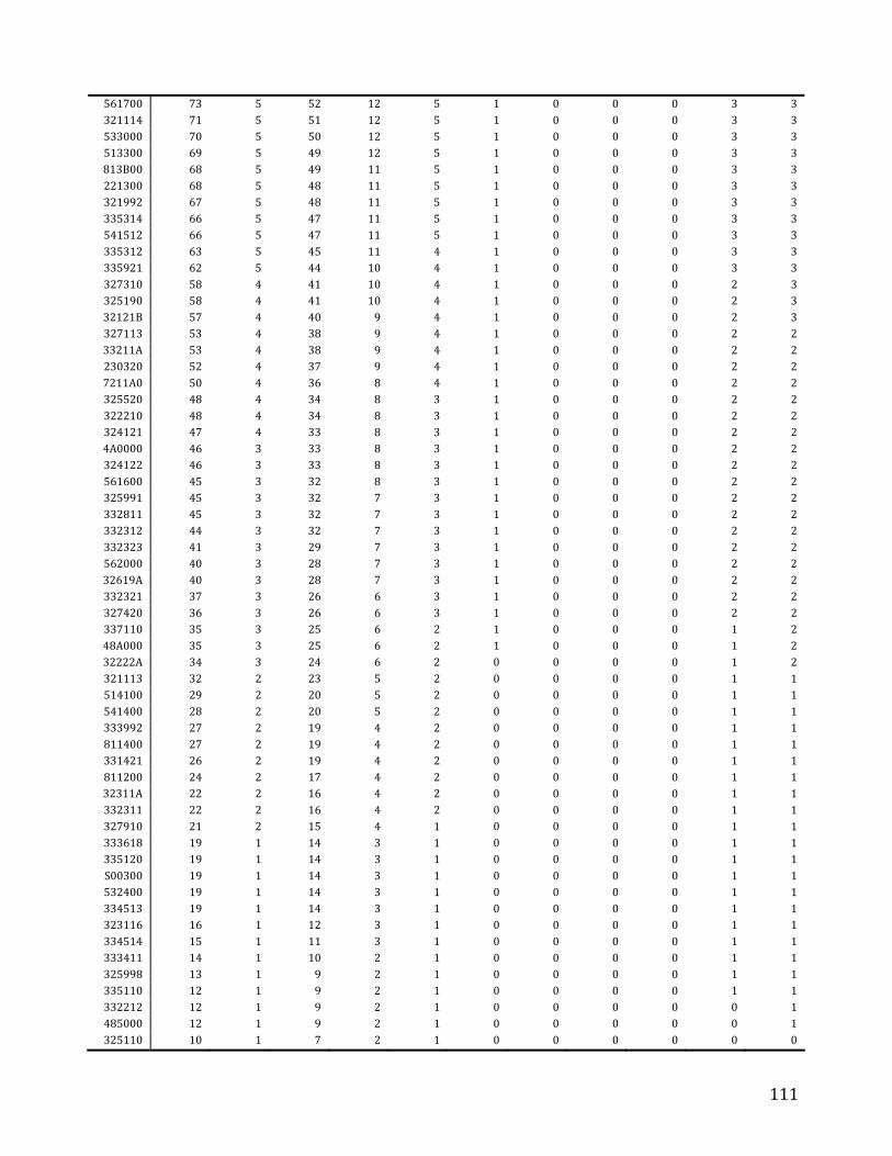
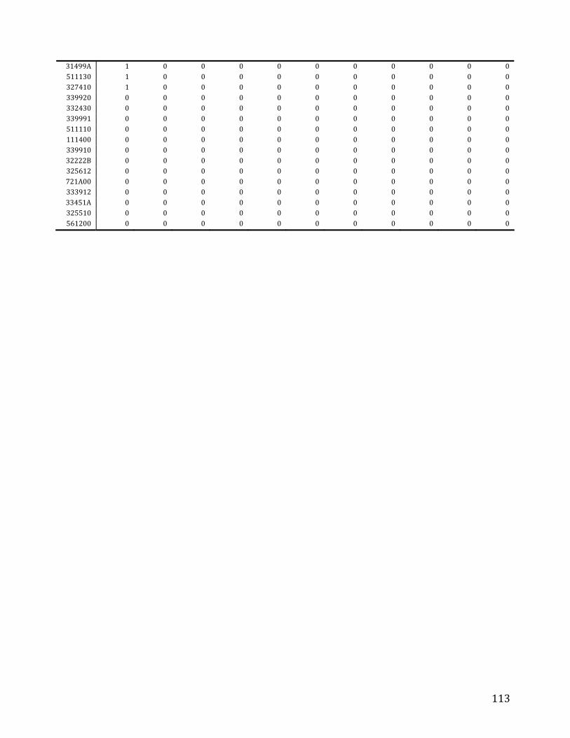
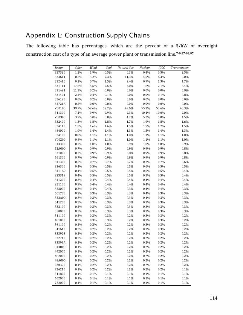
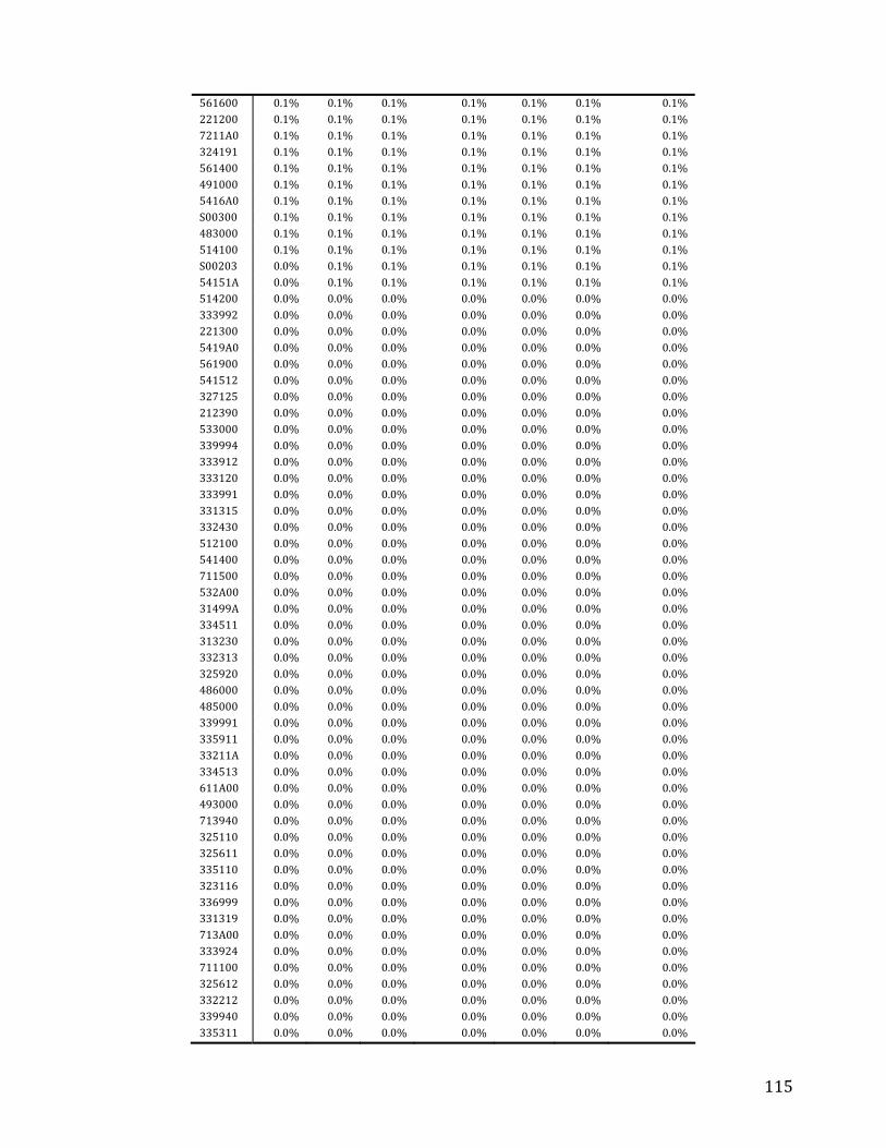
References 91 Appendix A: Original Distance Matrix (Chapter 2) 97 Appendix B: Modified Distance Matrix (Miles) 98 Appendix C: Completed Optimization, showing electricity transferred in TWh 99 Appendix D: Top 10 Sectors for each Generation Type 100 Appendix E: State Consumption Mixes 101 Appendix F: C++ Matrix-write Code 102 Appendix G: MATLAB Code – BuildIOModel.m 104 Appendix H: MATLAB Code – LoadUse.m 107 Appendix I: MATLAB Code – LoadMake.m 108 Appendix J: MATLAB Code – DoLCA.m 109 Appendix K: Disaggregated O&M Supply Chain 110 Appendix L: Construction Supply Chains 114
Page 8
v
List of Tables Table 1: Economic and global warming potential (GWP) contribution ix
Table 2: Comparison of California Energy Commission Net System Power 24
Table 3: Electricity Mixes for top 10 electricity importers 25
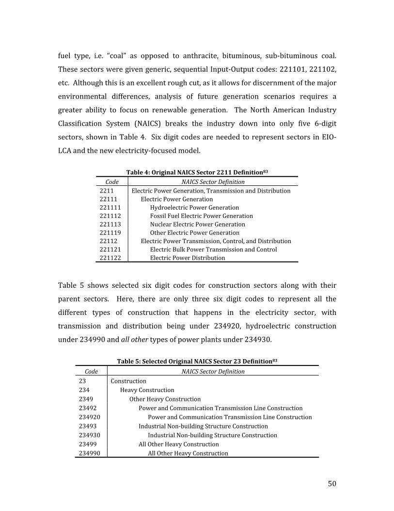
Table 4: Original NAICS Sector 2211 Definition83 50
Table 5: Selected Original NAICS Sector 23 Definition83 50
Table 6: PG&S O&M Sector Redefinitions 51
Table 7: PG&S Construction Sector Redefinitions 51
Table 8: Electricity O&M prices by Generation type ($1997/kWh) 7,8,86-93 54
Table 9: 1997 Benchmark use table for PG&S3 55
Table 10: Assumption-based allocation across generation types 56
Table 11: Priced-based Default Allocation 58
Table 12: Default allocation, with transmission and distribution accounted for 60
Table 13: Use table PG&S intersection allocation ($M) 61
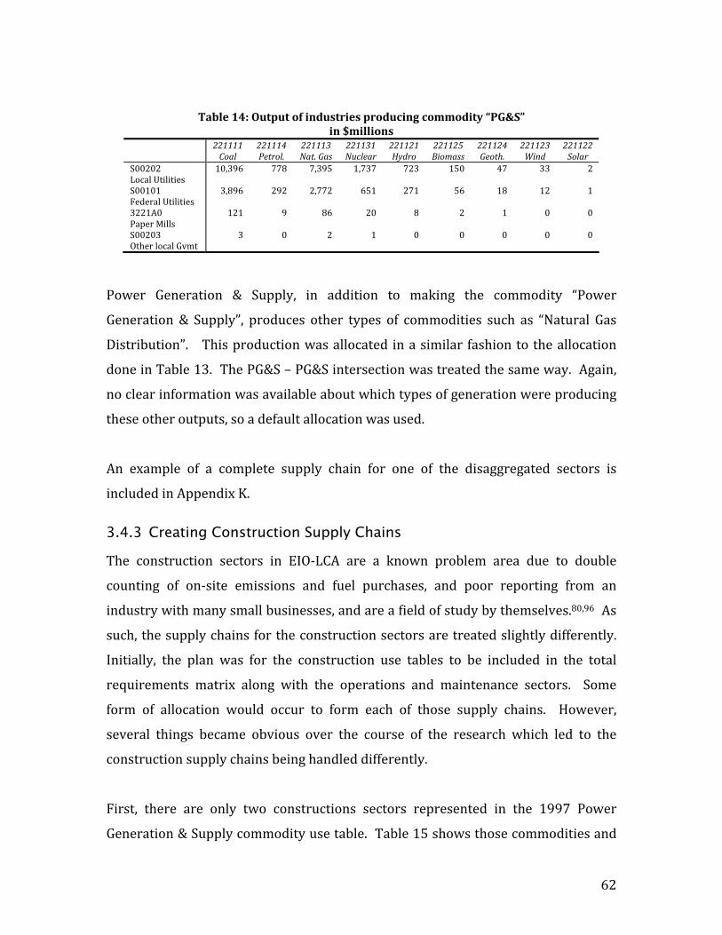
Table 14: Output of industries producing commodity “PG&S” 62
Table 15: Construction sectors in 1997 PG&S Use table, in $ billions3 63
Table 16: Selected 1997 heavy construction sector supply chains, in billions3 64
Table 17: Fraction of materials vs. services for construction 67
Table 18: Average emission factor ranges in tons/GWh13,39 68
Table 19: Construction Emission Factors, in lbs/$ 70
Table 20: 2005 Electricity Production Scenario Average Assumptions1 75
Page 9
vi
List of Figures Figure 1: Reported US electric utility O&M revenues and expenses, in $Billions1,2 viii
Figure 2: Electricity sales to all sectors with projections to 2050(PWh)7,8 x
Figure 3: 2005 U.S. electricity generation mix, in % of generated kWh1 xi
Figure 4: Natural Gas Price (Wellhead, 1994 $/tcf) 3
Figure 5: Average Annual Wind Power in the United States35 5
Figure 6: Life Cycle Stages43 6
Figure 7: Phases of a life-cycle assesment48 7
Figure 8: Calculating a consumption mix for the "Widget" manufacturing 15
Figure 9: State Electricity Generation Mixes versus US Average Mix for 200039 16
Figure 10: California & Western US Net Electricity Exports (TWh) 39 19
Figure 11: California Transfers from Optimization Model (TWh) 22
Figure 12: Creating a State Mix – Example 23
Figure 13: New Consumption Mix versus Old Generation Mix for California 24
Figure 14: Calculating difference between mixes 26
Figure 15: Difference measure of sector mixes to US average mix 27
Figure 16: Sector Consumption: Aircraft Manufacturing 30
Figure 17: CO2 (metric tons (MT)) from electricity used by Aircraft Manufacturing 34
Figure 18: CO2 (MT) from electricity used by Coal Mining 35
Figure 19: CO2 (MT) from electricity used by Automobile Manufacturing 36
Figure 20: CO2 (MT) from electricity used by Retail 36
Figure 21: Percent difference of CO2 compared to US Average Mix 37
Figure 22: Change in CO2 emissions from direct purchase of electricity 38
Figure 23: Change in CO2 emissions from total electricity purchases 40
Figure 24: Disaggregating the Power Generation & Supply Sector 42
Figure 25: Fossil-fuel prices paid by Electricity Generators1 53
Figure 26: Electricity O&M Prices by Generation Type7,8,86-93 54
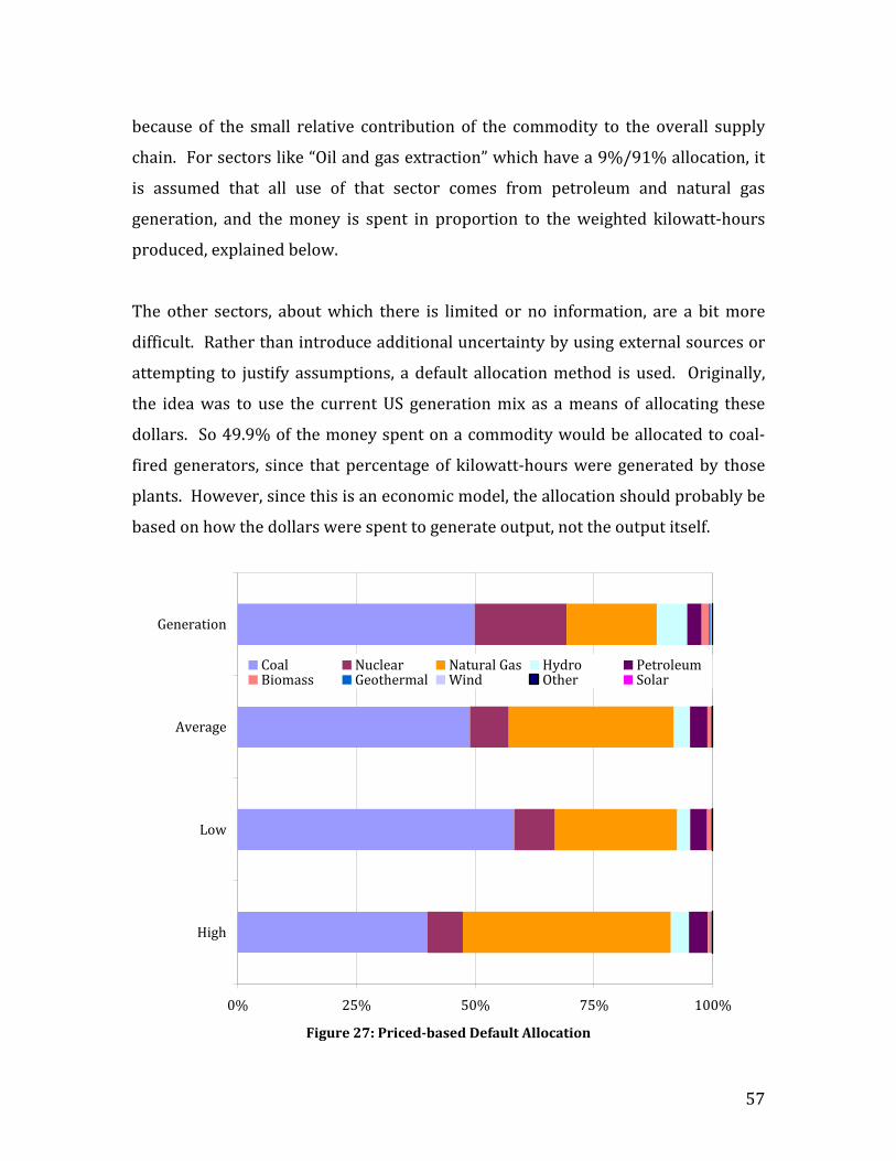
Figure 27: Priced-based Default Allocation 57
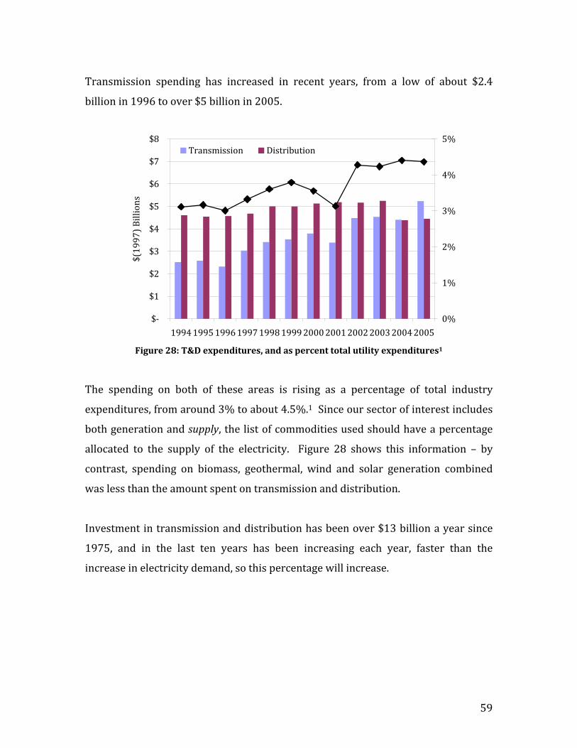
Figure 28: T&D expenditures, and as percent total utility expenditures1 59
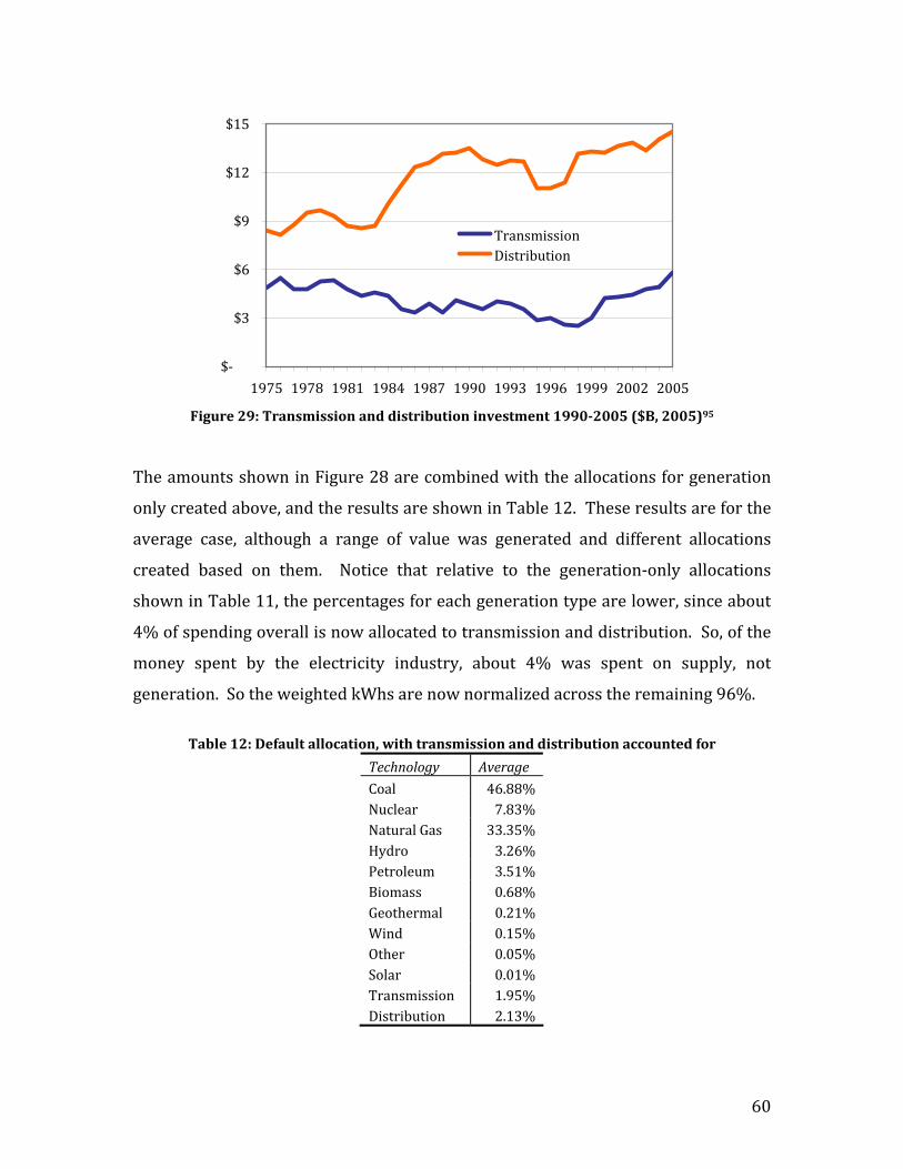
Figure 29: Transmission and distribution investment 1990-2005 ($B, 2005)95 60
Page 10
vii
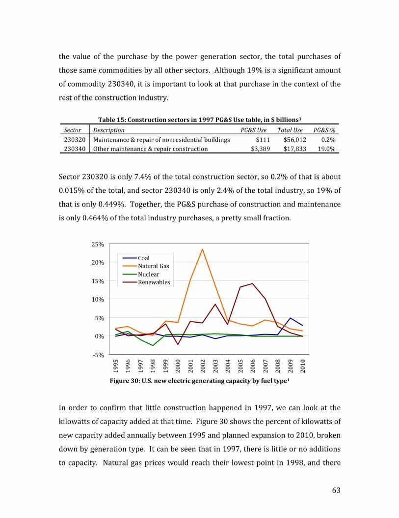
Figure 30: U.S. new electric generating capacity by fuel type1 63
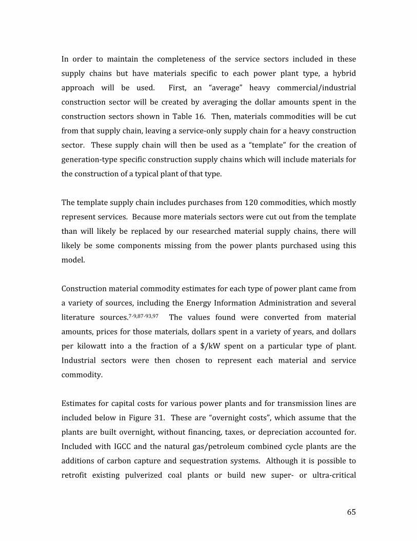
Figure 31: Overnight capital costs for new construction, 1997 $/kW7,8,87-93,98 66
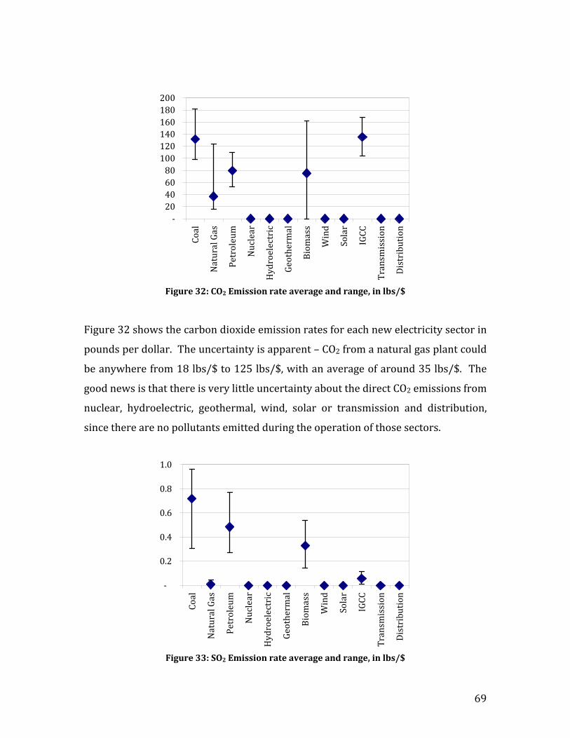
Figure 32: CO2 Emission rate average and range, in lbs/$ 69
Figure 33: SO2 Emission rate average and range, in lbs/$ 69
Figure 34: NOx Emission rate average and range, in lbs/$ 70
Figure 35: Economic comparison for 2005 generation, in $billions 77
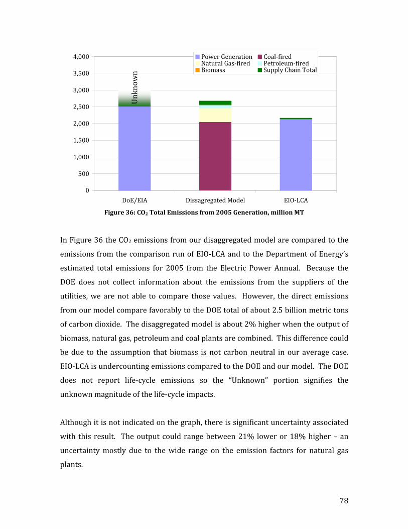
Figure 36: CO2 Total Emissions from 2005 Generation, million MT 78
Figure 37: NOx Total Emissions from 2005 Generation, million MT 79
Figure 38: SO2 Total Emissions from 2005 Generation, million MT 80
Figure 39: CO2 from power generation in 2040, in billion MT 82
Figure 40: CO2 from 2040 scenario, separating carbon from electricity 83
Page 11
viii
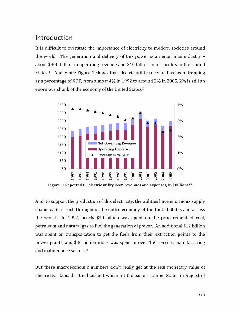
Introduction It is difficult to overstate the importance of electricity to modern societies around
the world. The generation and delivery of this power is an enormous industry –
about $300 billion in operating revenue and $40 billion in net profits in the United
States.1 And, while Figure 1 shows that electric utility revenue has been dropping
as a percentage of GDP, from almost 4% in 1992 to around 2% in 2005, 2% is still an
enormous chunk of the economy of the United States.2
$0
$50
$100
$150
$200
$250
$300
$350
$400
1992
1993
1994
1995
1996
1997
1998
1999
2000
2001
2002
2003
2004
2005
0%
1%
2%
3%
4%
Net Operating RevenueOperating ExpensesRevenue as % GDP
Figure 1: Reported US electric utility O&M revenues and expenses, in $Billions1,2
And, to support the production of this electricity, the utilities have enormous supply
chains which reach throughout the entire economy of the United States and across
the world. In 1997, nearly $30 billion was spent on the procurement of coal,
petroleum and natural gas to fuel the generation of power. An additional $12 billion
was spent on transportation to get the fuels from their extraction points to the
power plants, and $40 billion more was spent in over 150 service, manufacturing
and maintenance sectors.3
But these macroeconomic numbers don’t really get at the real monetary value of
electricity. Consider the blackout which hit the eastern United States in August of
Page 12
ix
2003. This outage affected 8 states – about 40 million people – for a period of less
than 24 hours, yet is estimated to have caused between $4 and $10 billion in
damages and lost productivity, or nearly a quarter of the annual profit of the entire
industry.4
And yet, these economic numbers pale in comparison to the large role that
generation and consumption of electricity plays in the environment. The raw
tonnage of a myriad of pollutants that the burning of fossil fuels expels into the
atmosphere is large, but difficult to comprehend. More easily grasped is how
inordinately large the environmental impact of power generation is compared to its
economic impact. In the coal mining industry in the United States, for instance, a
little over 1% of supply chain dollars go towards the purchase of electricity, yet this
purchase accounts for over 6% of the global warming potential (GWP) measured in
tons of CO2 equivalents associated with the operation of the mine and all suppliers.5
This effect, where the total national environmental impacts are six or more times
the economic impact, holds true for other types of emissions and pollution, and, as
seen in Table 1, for other types of industries as well. Indeed, for aircraft
manufacturers, the environmental impact as measured by global warming potential
is nearly 50 times that of the economic impacts of the electricity purchased, and
over 50 times for wineries.
Table 1: Economic and global warming potential (GWP) contribution
of power generation to major industrial sectors5
$ GWP
Coal mining 1.3% 6.3%Aircraft manufacturing 0.6% 27.7%Semiconductor manufacturing 0.8% 29.1%Wineries 0.7% 37.7%Primary aluminum 6.1% 48.2%
These emissions have world-wide reach and impacts. Electricity generation
accounts for nearly a third of the carbon in the atmosphere, as levels have risen
from 275ppm to 380ppm.6 And use of electricity, and the continued accumulation
Page 13
x
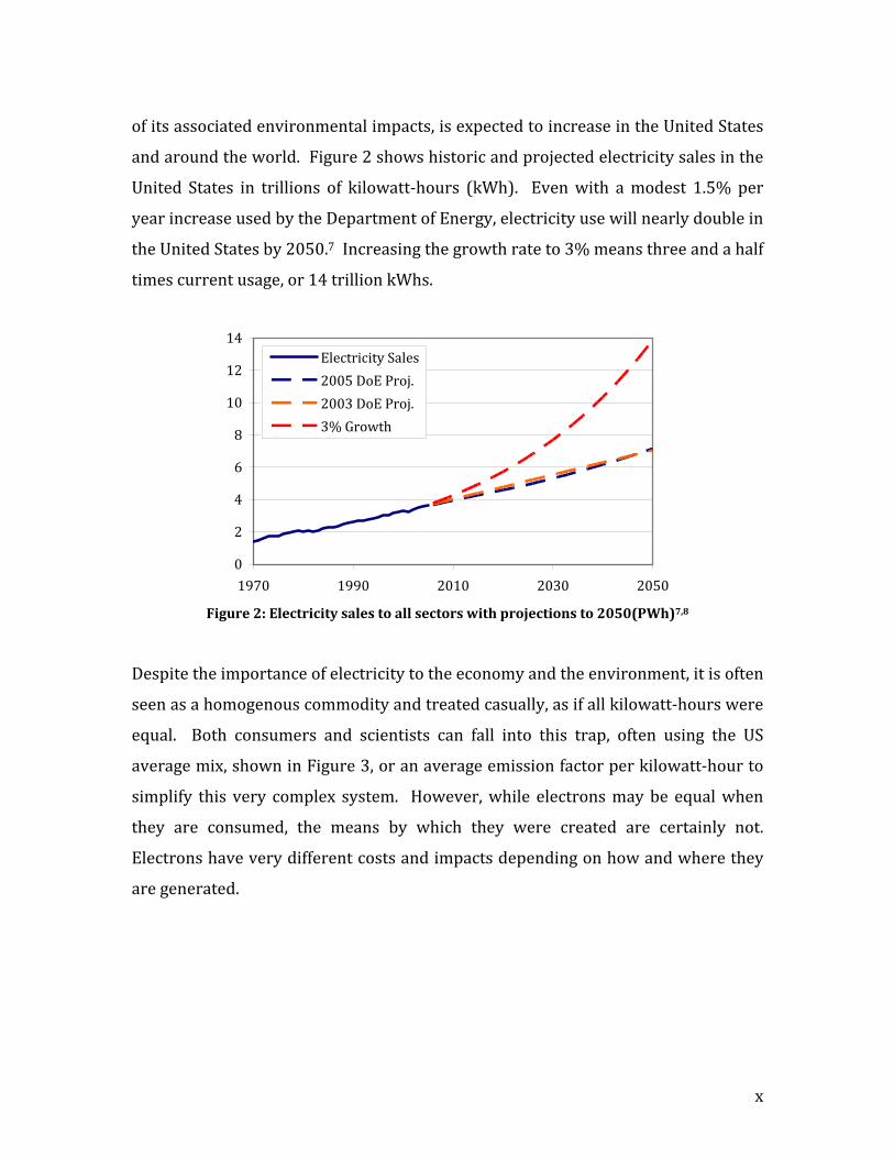
of its associated environmental impacts, is expected to increase in the United States
and around the world. Figure 2 shows historic and projected electricity sales in the
United States in trillions of kilowatt-hours (kWh). Even with a modest 1.5% per
year increase used by the Department of Energy, electricity use will nearly double in
the United States by 2050.7 Increasing the growth rate to 3% means three and a half
times current usage, or 14 trillion kWhs.
0
2
4
6
8
10
12
14
1970 1990 2010 2030 2050
Electricity Sales
2005 DoE Proj.
2003 DoE Proj.
3% Growth
Figure 2: Electricity sales to all sectors with projections to 2050(PWh)7,8
Despite the importance of electricity to the economy and the environment, it is often
seen as a homogenous commodity and treated casually, as if all kilowatt-hours were
equal. Both consumers and scientists can fall into this trap, often using the US
average mix, shown in Figure 3, or an average emission factor per kilowatt-hour to
simplify this very complex system. However, while electrons may be equal when
they are consumed, the means by which they were created are certainly not.
Electrons have very different costs and impacts depending on how and where they
are generated.
Page 14
xi
Coal, 49.9%
Nuclear, 19.3%
Natural Gas, 19.0%
Hydro, 6.4%
Petroleum, 3.0%
Biomass, 1.5%
Geothermal, 0.4%
Wind, 0.4%
Other, 0.1%
Solar, 0.0%
Figure 3: 2005 U.S. electricity generation mix, in % of generated kWh1
Because of electricity’s critical role in the economy, and less positive, but equally
potent role in affecting the environment, decision and policy makers at all levels are
interested in what’s currently happening and what’s going to happen with the
power generation industry, and just as importantly, how the rest of the economy
will respond to changes in the power generation sector. Both day-to-day and future
decisions regarding energy policy require the most complete information possible –
analyses which take into account supply chains and the connectedness of the
electricity sector to other areas of the economy.
There are quite a few examples in the electricity sector alone of “hidden” life-cycle
and supply chain environmental costs. The large amount of methane released by
flooded biomass behind conventional hydroelectric dams,9 the thousands of miles of
transmission lines and backup storage needed with large-scale wind generation10,11
or the large amount of toxic releases associated with the production of photovoltaic
solar cells are just a few of these examples.12
In her 2005 thesis, Bergerson showed that in certain potential high electricity
demand futures, such as those shown in Figure 2, even with 90% point-source
carbon capture on fossil power plants, the upstream, indirect, supply chain carbon
Page 15
xii
emissions like those associated with coal mining and rail transportation approached
current direct emissions from power plants and were greater than emissions from
other sectors of the economy such as transportation.13 The policy implications of
this are enormous – we stand little chance of ever approaching Kyoto Protocol-like
carbon levels if the supply chains of power generation produce that much carbon.
This is a major, unexpected supply-chain result. In the future, we’d like to be able to
make decisions about capital investment in generation methods and transmission
and distribution assets as well as operations choices – confident that we haven’t
overlooked major contributions from the supply chains of those choices.
In addition, as decisions are made in other industrial and commercial sectors about
the use of electricity – the purchase of power as part of the supply chain or life cycle
– it is important not to view it as a homogeneous quantity. The tools available to
policy makers to look at the complex problem of economics and emissions from
electricity generation and use in the future are varied.14,15 Unfortunately, these
tools, such as the Environmental Protection Agency’s MARKAL (Market Allocation)
model or the Department of Energy’s NEMS (National Energy Modeling System),
tend to be either complex and data intensive – requiring extensive expertise to use,
or are overly simplified, with data about electric utilities aggregated at too high a
level to be useful. 16-19
In the 500 sector input-output model of the US economy built by the Bureau of
Economic Analysis, power generation and supply are aggregated into a single sector.
By contrast, so are the impacts associated with tortilla manufacturing. A very
diverse set of technologies and supply chains are represented in this single
electricity sector. Comparing a kWh of electricity generated with hydro power to a
kWh generated using coal power is difficult when the economics and emissions
involved are so different – this difference is exacerbated when the supply chains are
taken into account as well.
Page 16
xiii
The model and results described in the following chapters provides a new level of
economic and environmental detail to decision makers, tied to the very simple
metric of dollars.
Page 17
1
1 Background This chapter covers the background information which is helpful in understanding
the work that follows in subsequent chapters. It includes sections on the power
industry, and generation in particular; and life-cycle inventory and assessment.
1.1 Power Generation & Supply As was discussed in the Introduction, the electricity sector is a very important one.
It is also very complex, made up of hundreds of public and privately owned utilities,
ranging in size from a few hundred to hundreds of thousands of customers. Its
primary roles are the generation, transmission and distribution of electricity, and in
some cases, steam heat.
Because of the industry’s importance, it is the subject of intense scrutiny and
research, by government, private and academic institutions. The body of work
looking at the myriad of issues is large, and expanding in both depth and breadth.
The background provided here is intended to briefly describe some of the major
issues associated with the major generation types and with transmission and
distribution. It is not intended to be either definitive or ground-breaking.
As delivering electricity was becoming economically viable in the waning decades of
the 19th century, it also became clear that there would be natural monopolies
because of the large infrastructure cost of producing and distributing the power.
For nearly one hundred years, the industry operated as a government-regulated
monopoly, and during this period the industry saw incredible growth, and the
United States saw nearly 100% electrification, even in far-flung rural areas. As
sprawling and interconnected as that system was, in the past 15 years, the industry
has been deregulated, and the complexity has increased accordingly.20
Coal-fired generators produced 50% of the electricity used in the United States in
2005.1 Coal is cheap, abundant, and available domestically, and so is expected to
Page 18
2
continue to play a large role in providing base-load capacity. It is, however, a non-
renewable resource, and the burning of coal causes damage to the environment in
the mining, transportation and, most significantly, combustion phases. Although
there are many regulations focused on cleaning up the output from this form of
generation, there is still a large amount of NOx, SOx, particulate matter (PM) and
volatile organic compounds (VOCs) emitted along with carbon and the less
abundant, but more toxic lead and mercury.21
Nearly all of the coal-fired plants in the US are pulverized coal, or PC, plants. The
coal is ground into a powder which is blown into a boiler to produce heat for
producing steam. These plants have become more reliable over time, with average
capacity factors around 60%22, but the process is very inefficient, extracting
between 30 and 35% of the input energy into usable electricity. Increased “tailpipe”
environmental controls such as flue gas desulphurization (FGD) or selective
catalytic reduction (SCR) further reduce this number.23
A newer technology with the potential for significant reduction in environmental
impacts is IGCC, or integrated coal gasification combined cycle. In these plants, the
pulverized coal – low sulfur coal is preferred in most gasifiers – is mixed with
oxygen under high temperatures to produce a mixture of hydrogen, carbon
monoxide, and methane,24 which is then burned in a combined-cycle turbine, where
the hot gases are used to spin one turbine, and the excess heat is used to create
steam to spin a second turbine, thereby extracting more useful energy.25 It is
possible to remove sulfur and other pollutants from the fuel stream prior to
combustion, making IGCC a cleaner use of a dirty fuel.26,27 IGCC plants are more
versatile as well; they can be used as either base load or load following plants, and
the gasified coal can be used as a fuel or feedstock for other industrial processes.28
Natural gas-fired power plants, either as single-cycle (gas turbine only) or
combined-cycle (gas and steam turbines) produced 19% of the electricity in the
Page 19
3
United States in 2005, although natural gas power plants made up almost 40% of
the installed capacity that same year.1 This results in a lower average capacity
factor, although this is tied more to the economics of producing power with high
priced natural gas than the reliability of the combined cycle plants. Natural gas
power plants produce electricity at a higher efficiency – between 50 and 60% for
combined-cycle plants – than their sub-critical coal-fired counterparts, and do so
with fewer emissions of NOx, SOx, carbon dioxide and particulate matter.
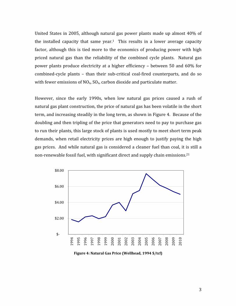
However, since the early 1990s, when low natural gas prices caused a rush of
natural gas plant construction, the price of natural gas has been volatile in the short
term, and increasing steadily in the long term, as shown in Figure 4. Because of the
doubling and then tripling of the price that generators need to pay to purchase gas
to run their plants, this large stock of plants is used mostly to meet short term peak
demands, when retail electricity prices are high enough to justify paying the high
gas prices. And while natural gas is considered a cleaner fuel than coal, it is still a
non-renewable fossil fuel, with significant direct and supply chain emissions.21
$-
$2.00
$4.00
$6.00
$8.00
1994
1995
1996
1997
1998
1999
2000
2001
2002
2003
2004
2005
2006
2007
2008
2009
2010
Figure 4: Natural Gas Price (Wellhead, 1994 $/tcf)
Page 20
4
In 2005, 19.3% of US power was generated with nuclear steam plants. Running at
capacity factors of over 90% in many cases, these power plants make up a
significant portion of the base load capacity. Nuclear electricity has very few local
emissions, although uranium and other heavy metals are present in small amount
from effluent streams.29 The nuclear life-cycle is important. Uranium, while
generally abundant in the earth’s crust and energy intense when concentrated, is
usually available in dilute amounts, and the enrichment of the fuel takes significant
amounts of energy. And, when the fuel is spent, it is thermally and radioactively hot,
and is currently stored at the plant site, with some sites holding nearly 50 years of
radioactive material.30 Until a national nuclear fuel repository like Yucca Mountain
is opened, the future of nuclear power in the United States will be uncertain,
although several utilities are beginning the long licensing process necessary to
install new, passively safe nuclear reactors.31 These plants are expensive, even
compared to the massive capital costs of other central generation projects.32
Although it is considered renewable, there are many environmental and social
implications of the 6.4% of electricity generated with hydropower. In hydropower,
water under high pressure (from gravity and water weight) spins turbines which
spin generators. There are other benefits as well – in addition to the electricity,
dams and the lakes behind them provide flood control, space for recreation, and a
reliable water supply (to some) for municipal, industrial and agricultural needs. But
hydroelectric dams, especially large scale canyon dams like those in the western US,
dramatically alter the ecosystem wherever they are built as well as incurring a large
impact during the construction and from biomass decay in the reservoir.9 In
addition, water “controlled” and held upriver is unavailable for use – for power,
drinking or irrigation – to those downstream. The water that is available is fast
moving, cold and devoid of nutrients and sediments which a river picks up along its
course. No new large-scale hydropower is planned in the United States, although
the potential exists for small “run-of-river” micro-turbines that would provide a
small amount of power, but have little ecological impacts.
Page 21
5
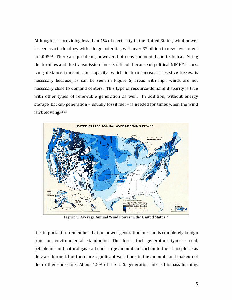
Although it is providing less than 1% of electricity in the United States, wind power
is seen as a technology with a huge potential, with over $7 billion in new investment
in 200533. There are problems, however, both environmental and technical. Siting
the turbines and the transmission lines is difficult because of political NIMBY issues.
Long distance transmission capacity, which in turn increases resistive losses, is
necessary because, as can be seen in Figure 5, areas with high winds are not
necessary close to demand centers. This type of resource-demand disparity is true
with other types of renewable generation as well. In addition, without energy
storage, backup generation – usually fossil fuel – is needed for times when the wind
isn’t blowing.11,34
Figure 5: Average Annual Wind Power in the United States35
It is important to remember that no power generation method is completely benign
from an environmental standpoint. The fossil fuel generation types - coal,
petroleum, and natural gas - all emit large amounts of carbon to the atmosphere as
they are burned, but there are significant variations in the amounts and makeup of
their other emissions. About 1.5% of the U. S. generation mix is biomass burning,
Page 22
6
which is generally considered carbon neutral.36 There is a small but growing
amount of wind and solar power – although expensive37 – used in the United States.
A major stumbling block is investors understanding of the future regulatory and
policy environment – technical aspects are not the issue38. Geothermal, waste-to-
energy plants, and “other fossil fuels” such as used tires are growing as well.39 The
impacts of these types are diverse, and certainly none is perfect.21,40-42
1.2 Life-cycle Inventory & Assessment Life-cycle assessment, or life-cycle analysis, is a framework which captures the
effects of all phases of the life of a product, service or sector: production,
transportation, use and maintenance, and disposal (Figure 6). This is sometimes
referred to as a cradle-to-grave analysis. LCA has been embraced by the
environmental community, but it is not limited to that type of analysis. Similar
assessments could be done to calculate the number of deaths caused by a product
over its lifetime, or the number of sheets of paper consumed by an industrial sector.
We are primarily concerned with LCAs done for environmental analysis here.43-45
Life-cycle inventory, or LCI, encompasses all of the data gathering steps associated
with LCA, but stops short of doing analysis of what that data means, either to the
environment or the economy. These steps are shown in Figure 7.
Figure 6: Life Cycle Stages43
Page 23
7
In an attempt to formalize a very open and general framework, several
organizations have developed standards for LCA, including the Society for
Environmental Toxicology and Chemistry (SETAC), the Environmental Protection
Agency and the International Standards Organization, as part of the ISO 14040
Environmental Management Systems standards.46,47
Figure 7: Phases of a lifecycle assesment48
Here we are concerned with three basic types of LCA: process LCA, Economic Input-
output LCA, and hybrid LCAs, which are described below.
1.2.1 Process LCA
A process LCA is concerned with unit processes, such as a the production of 1 ton of
copier paper, or 10,000 automobiles. Mass and energy balances are then done for
each phase in the life-cycle of that unit. A critical step in this process is the
identification of the boundaries and scope of the problem. For instance, you would
include the energy required to run the assembly line for the automobile, but would
you include energy required to produce the raw steel and aluminum, or the
production of the robots doing the work?
Page 24
8
Process LCA is a bottom-up method, and because of the large effort required to
gather input and output data for each step in the process, it is necessary to draw an
(arbitrary) boundary to reduce the complexity of the assessment. Significant
portions of the supply chain and many upstream uses are neglected, leading to
incomplete assessments or high costs.43 It is difficult and controversial to choose
between completeness and practicality. Varying boundaries for similar products
lead to problems with comparisons and lead to an overall impression that LCA is
more of an art than a science.
In addition, most process LCAs today are done using proprietary software and data,
meaning that assumptions and boundary choices are not transparent to those who
view the results.
1.2.2 EIO-LCA
In a reaction to the inherent complexity of process-based LCA, and also to
compensate for the issue of drawing the analysis boundary, a top-down economic
input-output method for doing environmental assessment was set forth by Wassily
Leontief, based on methods originally developed for macroeconomic analysis.49-51
The Economic Input-Output Life-cycle Analysis, or EIO-LCA, model , a workable and
publicly-available web-based tool developed by the Green Design Institute at
Carnegie Mellon University is a implementation of this method.52-55
EIO-LCA uses an 491-sector input-output model of the entire US economy, a model
which is made up of US Bureau of Economic Analysis 1997 survey data which
recorded what industries produced and what they purchased to produce it. The
main piece of the model is the (IA)1 matrix, or total requirements matrix, a
491x491 table of transactions, where each entry i,j is fraction of $1 spent on output
from industry i to produce $1 of output for industry j. The driving equation is:
E = X · (I – A)-1 · F
Page 25
9
where F is a vector of final demand in dollar terms, for instance, $5000 of copier
paper, or $200 million of cars, R is a vector of environmental stressors by sector and
E is the total environmental output, and the underlined piece is total demand,
including the supply chain.
The A matrix, as was said above, is made up of input and output data from
industries, but the survey information is processed through several steps first. To
build the A, a normalized “make” and a normalized “use” table are multiplied
together. The normalized make table is a representation of each commodity an
industry makes (outputs) as a fraction of total outputs created in a year. Likewise,
the normalized use table can be thought of as a supply chain – each industry another
industry purchases from (inputs) to produce its output as fraction of total inputs for
a year.56,57 These supply chains generally do not include construction or equipment
replacement because they are thought of as a capital investment outside of the
normal operation. However, a fraction of all capital investment is included as the
assets are manufactured inside the economy. Labor is included as value added,
rather than as a specific commodity.
The input-output tables are relatively easy to understand. Think of economy split
into about 500 industries and 500 commodities, so that the aircraft manufacturing
industry would make the commodity aircraft, etc. The make table shows which
commodities are made by which industries, and is generally pretty sparse. Because
there are mostly 1-to-1 relationships between industries and commodities (as with
aircraft manufacturing above), the diagonal of the make table is the only entry in
some columns and rows. There are exceptions, of course: an industry classified as
“auto parts manufacturing” might produce the commodity auto parts, but also farm
machinery parts.
The use table has many more values, and can be thought of as a series of supply
chains – the commodities which industries purchase to produce their output. Most
Page 26
10
sectors in the use table use hundreds of commodities and their output is in turn
used by dozens or hundreds of industries. There are circularities as well – a car
manufacturer might purchases a certain number of automobiles as part of the
operation.
The output from input-output models like EIO-LCA can be given in both direct and
indirect economic and environmental results. Direct results are the economic
activities and associated environmental outputs from the operation of the sector of
interest and its suppliers. Indirect results are the economic and environmental
activities associated with the operation of those supplier’s suppliers. Total output is
the sum of the direct and indirect outputs.
1.2.3 Hybrid LCA
One of the problems with using the current version of EIO-LCA as an analysis tool
for future electricity scenarios is the level of aggregation in the electricity sector.
Power generation of all types, construction, transmission and distribution are all
modeled as a single sector. As was said earlier, in this model, tortilla manufacturing
has the same sector representation as power generation and supply. The radically
different environmental impacts of fossil-fuel, nuclear and hydro generation are all
lumped together, or ignored. It is important to realize that this is a limit of the data
available from the BEA, and not of the framework or method.
Significant attention has been paid to input-output tables and their use in
macroeconomic analysis, which was the original purpose of input-output models.
There are many sources of uncertainty – the use of survey data as a basis, the
aggregation of millions of products and services into industrial sectors, changes to
the structure of the economy over time, marginal changes in demands which can
change the allocation of dollars in the model, etc.58,59 Making changes to the
structure of the a model with known uncertainty, and using it to model events 20 or
more years in the future, is in itself an uncertain undertaking. Current literature
shows us that if careful assumptions are made, the model is not particularly
Page 27
11
sensitive to small changes in structure or over time, although post-analysis should
be done to attempt to quantify the uncertainty.60
Even at the 500 sector level, there is significant aggregation that happens in input-
output analysis. A reaction to, and compromise for, this is hybrid LCA.
Hybrid LCA, as the name implies, is a combination of other forms of LCA. It is a
newly developed idea which seeks, in our case, to combine the comprehensive, but
high level, data of EIO-LCA with the detailed, low level information from a process
LCA. In an automobile LCA, you might use EIO-LCA to estimate economy-wide
discharges from the manufacturing phase and do a process LCA on the use phase of
the car.61-65
In our case, we are using the existing supply chains for 490 sectors, and adding
process-like detail to the Power Generation and Supply sector, so it could be
considered a hybrid LCA. The top-down EIO-LCA model has broad, highly
aggregated generalizations, and that is being combined with a bottom-up, or
technology rich, data with a detailed representation of changes in the electricity
sector. Combined, we can calculate broader effects throughout the economy with
regionally and/or functional disaggregated details
Page 28
12
2 Disaggregating Power Generation & Supply In order to create the information decision makers might need about the electricity
sector, and to accurately represent the vast differences among various methods of
generating electricity, economic and environmental information must be
disaggregated. This chapter will go through an analysis which shows why
disaggregating power generation and supply is important. A portion of this work is
previously published.66
As was said in the introduction , the emissions and other environmental stressors
from energy use, or, more specifically, from electricity generation, are significant
contributors to the total inventory in the life cycle assessments of many products,
processes or industry sectors. The environmental burden from this use occurs in
the form of air and water pollution, fuel and land consumption, and global warming
emissions. It is important to have good measures of these stressors in order to
quantify the possible implications for health, environment, and economy.
Many current product and process analyses that include the impacts of electricity
generation and consumption use aggregate, or average, data for the electricity
generation mix; all sectors consuming electricity are assumed to use the US average
generation mix, which is largely fossil-fuel based – over 50% coal and 70% fossil
fuels including natural gas and petroleum. These analyses might not do this
explicitly, but, as in the case of thousands of users of the Economic Input-Output
Life-Cycle Analysis tool developed at Carnegie Mellon5, they might just treat
electricity generation and consumption casually, without considering where the
facility being analyzed is located. A great deal of detail is lost at the state or facility
level since certain sectors – based on geographic location or purchasing choices –
buy and consume electricity with a very different generation profile than the more
aggregate, and fossil fuel-dominated, average mix. Perhaps the best example of this
would be the aluminum manufacturing sector, an industry which uses a lot of
electricity in its processes. While there are aluminum plants throughout the United
Page 29
13
States, a significant percentage, if not the majority, are located in the Northwest US,
particularly Oregon and Washington, where they take advantage of relatively low-
cost (and low emission) hydroelectric power. These states generated 94% and 88%
of their power with hydro, respectively, in 1997.39 So one would expect, if a
generation mix could be assigned on a sector by sector basis, that there would be
significant changes in the LCA output – the impacts associated with this industry,
such as lowering CO2 emissions estimates. Global warming, ecosystem disruption,
hazardous waste, and security – both energy and homeland – are elements that
must be considered. The cost to the environment and to human health from
electricity generation is large.
Disaggregating electricity generation, or splitting it up by primary energy source,
would allow assignment of a specific mix of generation types – and therefore a
specific mix of environmental effects – to each product or process. This is called a
consumption mix. In this chapter, we look at the results of one method of
disaggregation, and create an optimization model for interstate electricity trading to
improve its accuracy. The analysis highlights the overall importance of
disaggregating this sector and some unexpected results and the implications that
these results have for environmental impact assessment of electricity consumption.
2.1 Creating Consumption Profiles Ideally, to disaggregate and move away from using the US average mix for
environmental analysis, we would have, broken down by fuel type, the amount of
electricity that every industrial and commercial facility in the United States used.
An automobile manufacturing plant near Detroit, for instance, might have a
published “consumption mix” which would show that the electricity they consumed
was generated with 75% coal and 25% nuclear. Comprehensive consumption mix
data like this at the plant level would require synthesis of millions of power
transactions from thousands of firms. It would be necessary to collect the amount of
electricity each facility purchased from each supplier, and the type of generation
method those suppliers were using or purchasing themselves. Models would match
Page 30
14
supply and demand and allocate electrons via the various grid-connected entities of
different generation types based on values changing daily, if not more often. But
these numbers are not readily available; in general, contracts between utility
companies and their customers are confidential, even if the grid were metered at
that level. It is apparent that some level of geographic aggregation is necessary,
since the data needed to achieve complete disaggregation is not available.
We can make educated guesses about facility-level consumption mixes, based on the
idea that electrons flow from the closest available source. Carnegie Mellon
University in Pittsburgh, for instance, consumes power produced just down the Ohio
River at one of several large coal plants, and some from a nuclear plant from 30
miles away in Beaver Valley. We can make this statement because we know two
important things: 1) where Carnegie Mellon is located geographically, and 2) the
generation assets in that region. Similarly, if we can identify the location of
manufacturing facilities and combine that information with accurate regional
generation profiles, we can systematically produce consumption mixes for all
manufacturing sectors across the country.
Both pieces of information are readily available from public sources. Both the US
Department of Energy and the US Environmental Protection Agency provide yearly
state generation mixes (e.g., the percent of each generation type – coal, gas, nuclear,
etc. – generated in the state in a given year).39 The Bureau of Economic Analysis
collects census data for every industry sector in the US.67 We use the median
number of employees for each sector in a state as an indicator of presence in the
state, then divide by the total number of employees in that sector country-wide to
produce a percentage in that state.68 Other metrics of industry presence were
checked, including number of facilities and value of products shipped. Number of
employees correlated highly with value of products shipped and this type of data
was available for more sectors.
Page 31
15
Each industry sector then has a specific set of six percentage values assigned to it
(for coal, petroleum, gas, nuclear, hydro and other), which is a combination of
fractions of the generation mixes for each state that the sector has facilities in. In
some cases, sectors will have locations in all 50 states; in other cases, there will only
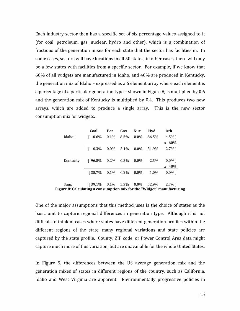
be a few states with facilities from a specific sector. For example, if we know that
60% of all widgets are manufactured in Idaho, and 40% are produced in Kentucky,
the generation mix of Idaho – expressed as a 6 element array where each element is
a percentage of a particular generation type – shown in Figure 8, is multiplied by 0.6
and the generation mix of Kentucky is multiplied by 0.4. This produces two new
arrays, which are added to produce a single array. This is the new sector
consumption mix for widgets.
Coal Pet Gas Nuc Hyd Oth
Idaho: [ 0.6% 0.1% 8.5% 0.0% 86.5% 4.5% ] x 60%
[ 0.3% 0.0% 5.1% 0.0% 51.9% 2.7% ] Kentucky: [ 96.8% 0.2% 0.5% 0.0% 2.5% 0.0% ] x 40%
[ 38.7% 0.1% 0.2% 0.0% 1.0% 0.0% ] Sum: [ 39.1% 0.1% 5.3% 0.0% 52.9% 2.7% ]
Figure 8: Calculating a consumption mix for the "Widget" manufacturing
One of the major assumptions that this method uses is the choice of states as the
basic unit to capture regional differences in generation type. Although it is not
difficult to think of cases where states have different generation profiles within the
different regions of the state, many regional variations and state policies are
captured by the state profile. County, ZIP code, or Power Control Area data might
capture much more of this variation, but are unavailable for the whole United States.
In Figure 9, the differences between the US average generation mix and the
generation mixes of states in different regions of the country, such as California,
Idaho and West Virginia are apparent. Environmentally progressive policies in
Page 32
16
California have created a generation mix that uses extremely small amounts of coal-
fired electricity, and large amounts of cleaner burning natural gas and low-emission
hydroelectric power. Or, as we’ll see later, these policies simply push coal
generation across the state’s eastern borders. California also has significant
amounts of geothermal, biomass and wind power, which is reflected in the “Other”
category. West Virginia, like several other states in the region, has large amounts of
coal available for mining, and this is apparent in its mix. Idaho, on the other hand,
has been able to generate nearly all of its power with hydroelectric dams.
0%
20%
40%
60%
80%
100%
United States California Idaho West Virginia
Coal PetroleumNatural Gas NuclearHydro Other
Figure 9: State Electricity Generation Mixes versus US Average Mix for 200039
Another simplifying assumption made so far in this method is that it does not take
into account interstate power sales. Not including interstate trading might have
been a valid assumption prior to large scale deregulation of the electricity industry,
enacted in 1994 and implemented first in 1998, but deregulation brings the
additional complication of states being able to purchase electricity not only from a
different state, but in fact from a particular company with a particular generation
type. For example, Carnegie Mellon University purchases 6% of its total electricity
as wind power from 75 miles away in Somerset County. While not in a different
Page 33
17
state, it illustrates the ability of consumers to choose their generation type,
regardless of state or regulatory borders69. In 2000, interstate net exports totaled
nearly 10% of the total electricity consumed in the United States39.
So, although regional variation in generation types are accounted for by the state
mixes, large power surpluses or deficits of electricity are not. Large amounts of
power moves across state borders from states with excess capacity to those with a
lack of electricity. California, the country’s largest consumer and importer, brought
in 26% of its power in 2000 – 67 terawatt-hours (TWh) worth. West Virginia
exported nearly 70% of the power generated in-state39. It appears that the inclusion
of import and export data has significant effects on the electricity consumed within
the state. California, for example, generates a little over 1% of its electricity with
coal, but it imports nearly 30% of the electricity it consumes, much of which is
probably generated in nearby coal-heavy states such as Arizona and Wyoming.
Surprisingly, data on which states shipped power and to whom is not readily
available. The National Energy Board in Canada publishes information about gross
inter-provincial electricity transfers70, but in the United States the only data
consistently available is the net generation number published by the EPA. Basically,
it is the state’s gross consumption for a particular year subtracted from its gross
generation. A negative number means the state is a net importer for the year; a
positive number indicates a net exporter. This does not mean that a net importer
exported no power. It is in fact quite likely that power was shipped out one border
and in another, but this is not indicated by the net values available. We don’t
attempt to “fix” this, since assumptions about gross imports and exports would
likely lead to a large amount of uncertainty and unverifiable results given the data
gaps described above.
Modeling all electricity flow across the grid in North America is not an easy task. It
is an incredibly complicated system with millions of components, constantly
Page 34
18
fluctuating supplies and demands, and hundreds of players attempting to maximize
their own benefit. Again, as with disaggregation itself, assumptions and
simplifications need to be made in order to make the problem tractable given the
data available.
In lieu of creating a perfect representation of the entire North American grid, a
model was made that approximated the grid’s high-level physical behavior rather
than a model based on the economic transactions that drive it. Consider again the
example of Carnegie Mellon University purchasing wind power: while the
university’s purchase drives demand for the wind generation plants, due to the
distance involved and the proximity of other local generation it is quite unlikely that
any of the power generated there is actually used by the university without a direct
link (a transmission line) between them. Power will flow over the grid to the closest
demand, or, more accurately, along the paths of least resistance, which, all other
things being equal, will be the shortest path. And the closest demand for Somerset’s
wind power is not 75 miles away in Pittsburgh, but likely in Somerset County itself.
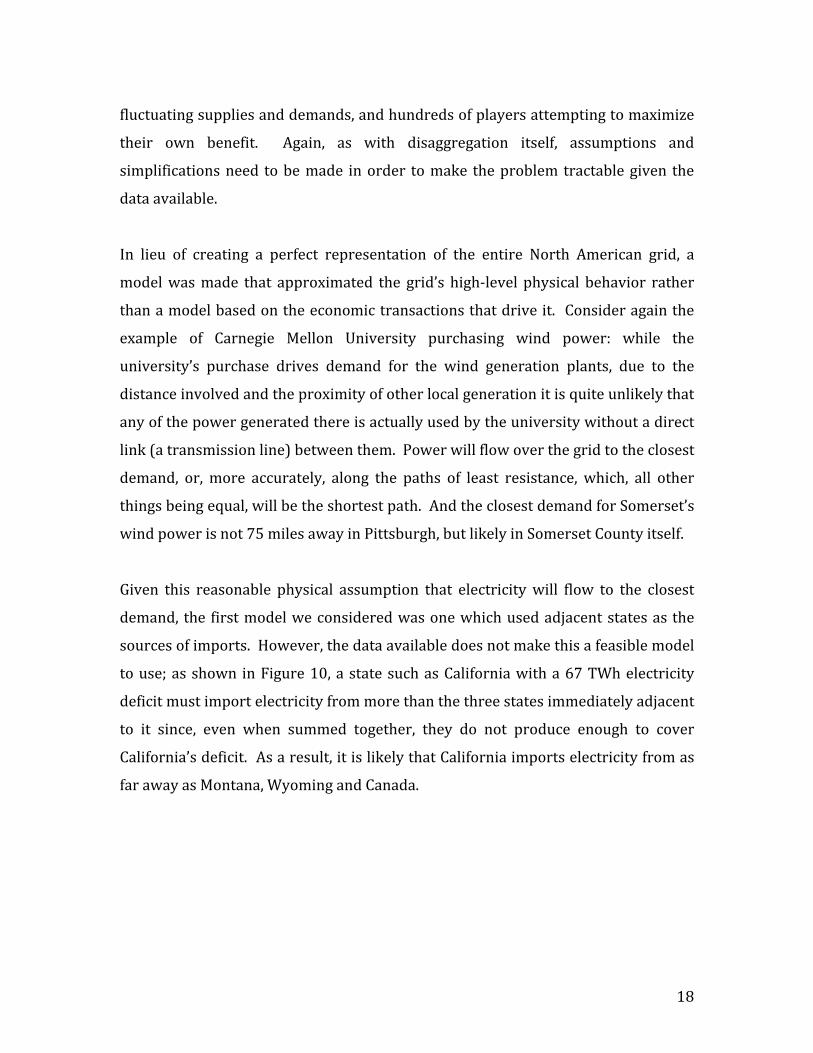
Given this reasonable physical assumption that electricity will flow to the closest
demand, the first model we considered was one which used adjacent states as the
sources of imports. However, the data available does not make this a feasible model
to use; as shown in Figure 10, a state such as California with a 67 TWh electricity
deficit must import electricity from more than the three states immediately adjacent
to it since, even when summed together, they do not produce enough to cover
California’s deficit. As a result, it is likely that California imports electricity from as
far away as Montana, Wyoming and Canada.
Page 35
19
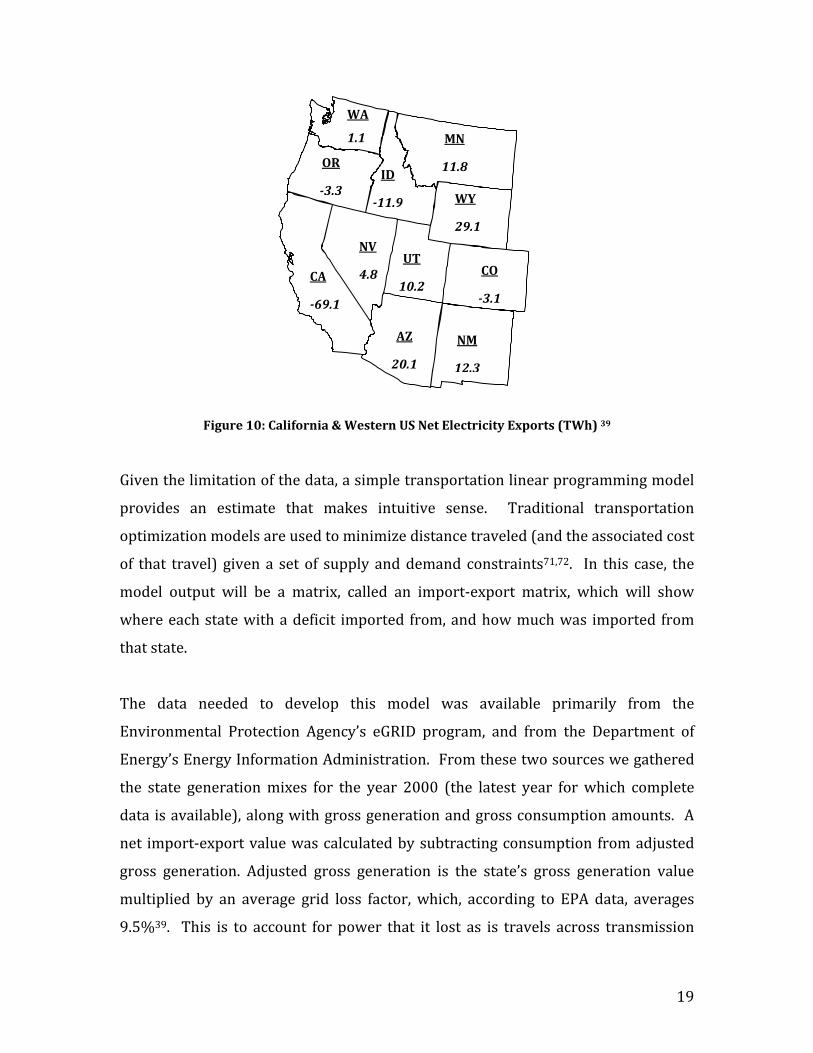
Figure 10: California & Western US Net Electricity Exports (TWh) 39
Given the limitation of the data, a simple transportation linear programming model
provides an estimate that makes intuitive sense. Traditional transportation
optimization models are used to minimize distance traveled (and the associated cost
of that travel) given a set of supply and demand constraints71,72. In this case, the
model output will be a matrix, called an import-export matrix, which will show
where each state with a deficit imported from, and how much was imported from
that state.
The data needed to develop this model was available primarily from the
Environmental Protection Agency’s eGRID program, and from the Department of
Energy’s Energy Information Administration. From these two sources we gathered
the state generation mixes for the year 2000 (the latest year for which complete
data is available), along with gross generation and gross consumption amounts. A
net import-export value was calculated by subtracting consumption from adjusted
gross generation. Adjusted gross generation is the state’s gross generation value
multiplied by an average grid loss factor, which, according to EPA data, averages
9.5%39. This is to account for power that it lost as is travels across transmission
CA
69.1
ID
11.9
OR
3.3
CO
3.1
NV
4.8 UT
10.2
MN
11.8
NM
12.3
AZ
20.1
WY
29.1
WA
1.1
Page 36
20
lines (before it can be consumed). A positive net import-export means the state had
an electricity surplus and a negative net import-export means that the state had a
deficit in 2000. In 2000, there were 27 importers and 27 exporters. The 54 total
entities included the 48 contiguous states, as well as the District of Columbia,
Canada, and Mexico; California, Mexico and Canada were counted as both importers
and exporters since gross data was available39.
This data provided the first part of the model, which was the suppliers (exporters),
customers (importers) and constraints (supplies and demands for each state). The
second portion of the data for the model was the distance between each importer
and exporter – a straightforward great circle distance between the entity’s
geographic centroids73. The full distance matrix is included in Appendix A.
In addition to this basic data, there were some additional elements of the power grid
we modeled, one of which was the presence of three (Western, Eastern and Texas)
managed interconnect regions in the United States and Canada. The borders for
these regions are complicated, but can be approximated with state boundaries. The
Texas interconnect region is basically the state of Texas, and the border between the
Western and Easter interconnect falls along the eastern border of the states shown
in Figure 10. There are few connections between interconnects, and in fact the
regions are asynchronous – the AC power is phased differently, making direct
transfer impossible. A DC tie line is needed to move power from one interconnect to
another. It would be unrealistic if the model moved large amounts of power
between the interconnect regions.
In order to reduce the amount of cross-interconnect transfer happening, but not
prevent it entirely, we reduce the distances between states within the same
interconnect by multiplying the distance by a certain factor, making it unlikely that
the model would move power between states not in the same interconnect. The
Page 37
21
factor we used was 0.1, or a 90% reduction. A series of factors between 0 and 1
were tested, and a lower factor proved more effective at preventing transfer.
In general, high voltage direct current, or HVDC, lines are put in place to facilitate
the movement of excess power from the generator to a place without enough
generation, and provide known electricity transfer “routes” which can be modeled.
But the linear optimization performs this task already, without the need to
artificially modify the distances to make it more likely that power will travel along
certain routes. And with the creation of ever larger AC transmission lines, it would
be necessary to create these lines in the model as well as DC lines. A decision was
made to keep the model simple rather than attempt to recreate the entire grid.
Finally, in order to modify the optimization to adhere to some limitations of the
data, certain adjustments were made. Canada is not allowed to ship power to
Mexico or vice versa, since the export data for Canada explicitly goes to the United
States. Further, all of Mexico’s imported power in 2000 came from California, so this
transfer is made a constraint in the optimization. California then has its total
electricity import increased by 2.1 TWh – the amount it transfers to Mexico. This
modified distance matrix is included in Appendix B.
When run, the optimization minimizes the sum product of the weighted distance
matrix and the import-export matrix, both described above, by modifying the values
in the import-export matrix. This minimized value is the total “cost” of moving
electricity from the exporters to the importers. It is subject to two main sets of
constraints: each row sum in the import-export matrix must be exactly equal to the
amount of excess power available in that state, and the column sums must be
exactly equal to the power deficit of that state.
The final results of the optimization for all states are included in Appendix C,
although the results for California are shown in Figure 11. This is a linear
Page 38
22
programming problem, so the result is the minimum cost that can be achieved with
the given constraints. But the results seem to make intuitive sense as well:
California imports from Arizona (29%), New Mexico (13%), Nevada (7%), Utah
(15%) and Wyoming (36%). All had large electricity surpluses, and are within the
Western interconnect.
Figure 11: California Transfers from Optimization Model (TWh)
With the values from the optimized import-export matrix, and knowing the amount
of electricity generated in the importing states, we can calculate a new electricity
mix, which we refer to as a consumption mix, for each state. It is found by
multiplying the percentage of imports received from each state by the generation
mix from that state (assuming that the electricity they export will follow the
generation mix for electricity used in-state) and multiplying that by the importing
state’s current generation mix.
In the example shown in Figure 12, the consumption mix for California is calculated
based on the results shown in Figure 11. We know the percentage of power
imported to the state, and this is broken out as percentages of the states which
NV
4.8UT
10.2
NM
9.2
AZ
20.1
WY
24.8
CA
2.1
Page 39
23
exported power to California. We therefore know the percentage of total
consumption that each import makes up. And since we know the original EPA
generation mixes for all the states in question, we can multiply each mix array by
the respective state’s percentage of consumption. By adding each generation type,
we can get a final consumption mix for California which includes all the imports
provided by the optimization.
Figure 12: Creating a State Mix – Example
The new generation mix for California is shown in Figure 13. The impact of the
large amount of coal imports from Wyoming, Utah and Arizona is obvious. Despite
the published generation mix for California’s which seems to promote clean air, the
results here suggest that California consumes almost 20% of its electricity overall
from coal-fired power plants. This would lead to an increase of over 30% in tons of
CO2 emitted from the burning of fossil fuels to generate electricity for California,
from 850,000 tons to almost 1.3 million tons39. And due to the general flow of air
and pollutants from west to east in the western United States, California doesn’t see
all the emissions resulting from this consumption.
Page 40
24
0%
10%
20%
30%
40%
50%
Coal Petroleum NaturalGas
Nuclear Hydro Other
GenerationConsumption
Figure 13: New Consumption Mix versus Old Generation Mix for California
Verification of the model results are difficult: the model was built because little data
about interstate trading were available. However, there is some high-level
aggregate information about where states get their power. Each year the California
Energy Commission (CEC) estimates its electricity imports and which region they
were was imported from. It separates the importers into three regions: Pacific
Southwest, Pacific Northwest, and Other74,75, and creates a Net System Power
calculation, which is similar to our consumption mix75,76. A summary of these values
is shown in Table 2; both are estimates, and the total difference is less than 20%.
Table 2: Comparison of California Energy Commission Net System Power
versus model calculated consumption mix76
CEC Net System Power
Model Results
Coal 15.7% 21.4%Natural Gas 35.1% 38.4%Petroleum 1.3% 1.0%Nuclear 17.2% 15.0%Hydroelectric 21.8% 15.0%Other 8.9% 9.2%
Some of the difference, especially the higher fossil fuel and lower hydroelectric
numbers in the trading model, are likely due to difference in the way the results
Page 41
25
were calculated. The CEC numbers are based on purchases that California utilities
make. The utilities purchase hydroelectric power from Oregon and Washington,
which run along dedicated north-south DC lines. These states are net importers,
however, so while they may be selling California their hydroelectric power, they are
in turn importing power from Idaho and Wyoming. A good amount of the excess
power in Wyoming is coal-fired. Our model cuts out the middle-man and assumes
that the coal-fired electricity is shipped directly to California.
The final import-export matrix and the new consumption mixes for each net
importer are included in Appendices C and E. A summary of the top 10 importers
and their new consumption mixes is included in Table 3. These new consumption
mixes for each importing state are combined with the original generation mixes for
each exporting state and are used in the same industrial sector disaggregation
process explained earlier, which assigns a consumption mix to each industrial
sector. In Table 3, the original 2000 state generation mix is on the top and the
consumption mix is below in italics.
Table 3: Electricity Mixes for top 10 electricity importers
Imported Amount (TW
h)
% Consumption Imported
Coal
Petroleum
Natural Gas
Nuclear
Hydroelectric
Other
Washington DC 10.5 99% 0% 100% 0% 0% 0% 0% 97% 1% 0% 0% 1% 0% Delaware 6 53% 69% 14% 14% 0% 0% 3% 63% 8% 7% 20% 0% 2% Idaho 11.9 52% 1% 0% 8% 0% 86% 4% 26% 1% 5% 0% 66% 3% Massachusetts 16.5 32% 29% 20% 27% 14% 6% 5% 36% 14% 19% 22% 5% 5% Virginia 30.1 30% 51% 4% 6% 36% 0% 3% 65% 3% 4% 25% 0% 2% Rhode Island 2 27% 0% 1% 97% 0% 0% 2% 15% 1% 71% 10% 0% 2%
Page 42
26
California 67 26% 1% 1% 50% 17% 19% 12% 21% 1% 38% 15% 15% 9% Mississippi 11.5 25% 37% 8% 22% 28% 0% 4% 41% 6% 18% 31% 0% 3% Maryland 15.4 25% 58% 5% 6% 27% 3% 2% 66% 4% 4% 22% 3% 1% New Jersey 17.5 25% 16% 2% 28% 50% 0% 3% 27% 2% 22% 47% 0% 3%
2.2 Analyzing Sector Consumption Profiles With the optimization and two sets of disaggregations complete, there are two sets
of data to compare. The first is the initial disaggregation which does not include
interstate electricity trading and the second includes the results of the import-
export model. Each set has 519 arrays of six percentages – one array for each US
industry sector. In order to assess the impact of disaggregation, we compare each of
these arrays to the 2000 average US generation mix, since, prior to disaggregation,
these are the values which were being used to calculate environmental impact.
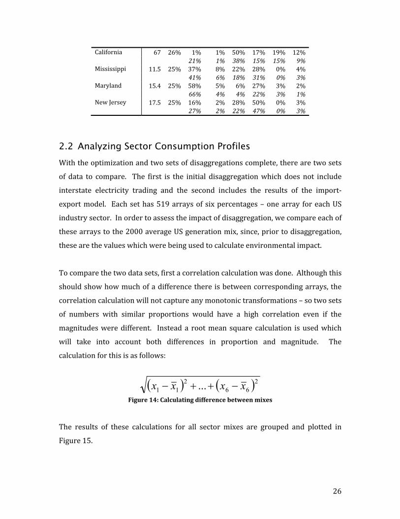
To compare the two data sets, first a correlation calculation was done. Although this
should show how much of a difference there is between corresponding arrays, the
correlation calculation will not capture any monotonic transformations – so two sets
of numbers with similar proportions would have a high correlation even if the
magnitudes were different. Instead a root mean square calculation is used which
will take into account both differences in proportion and magnitude. The
calculation for this is as follows:
( ) ( )266
211 ... xxxx −++−
Figure 14: Calculating difference between mixes
The results of these calculations for all sector mixes are grouped and plotted in
Figure 15.
Page 43
27
0
50
100
150
200
250
<10% 10-15% 15-20% 20-25% 25-30% >30%
Consumption Generation
Figure 15: Difference measure of sector mixes to US average mix
Before the analysis was begun we expected to see that disaggregation had a
significant impact on the consumption mixes for all industrial sectors. “Impact” in
this case was defined as a measure of how different the process-generated
consumption mix was from the originally assigned US average mix. We had further
expected that adding imports and exports would exacerbate this result: the
consumption mixes would be more different than the US averages. But analysis
done on the results of the disaggregation lead us to reject our initial hypotheses –
while some sectors have disaggregated consumption mixes quite different from the
US average, most are very similar to it. Additionally the inclusion of imports and
exports has an averaging effect, which makes consumption mixes more like the US
average rather than more different.
An important conclusion shown here is that most sectors have mixes which are
within 15% of the United States average mix, and very few of the sectors have mixes
which are more than 25% different. However, the tail of the distribution is quite
long – although it’s trimmed in Figure 15 – and knowing which sectors make up that
tail is important. Also, there is a definite shift to the left for the consumption as
opposed to the generation mix. This is because, as was said before, the trading of
power makes things look more like the average.
Page 44
28
The most likely explanation for the trend towards the average, both for the standard
disaggregation consumption mix and the disaggregation with trading consumption
mix, is spatial diffusion. Sectors spread out across the country will have profiles
much like the country itself. This is obvious for sectors such as restaurants,
hospitals and oil change shops. What is interesting is how many other sectors,
which we were not expecting to be diffused across the country actually are, or at
least appear to be, based on their consumption mixes with low differential index
values.
That interstate trading would have an averaging effect on consumption mixes
should have, in retrospect, been obvious. As states get power from a wider variety
of sources, the chances that those sources together will look like the US average
increases. When we look at some simple comparisons we can see this effect quite
clearly. Prior to including imports and exports, the three states most different from
the average were Idaho (due to large amounts of hydroelectric power), Rhode Island
(generates internally with mostly natural gas), and Hawaii (generates electricity
with petroleum). When the optimization was run, and the new generation mixes
were compared to the old, the two states that had changed the most were Idaho and
Rhode Island. Looking again at a comparison to the US average mix, but this time
using the new generation mixes, Rhode Island and Idaho are no longer even in the
top ten for difference from the average. The inclusion of imports made them more
like the average and dropped them out of the top spots. Overall, however, the effect
of adding imports and exports is small, with the total difference between the normal
disaggregate results and those including interstate trading being about 3%.
Although the difference in results for this particular use is small, it is still interesting
to be able to quantify the difference. This comparison would have been made much
easier with better data availability. Gross import and export data, such as that
available from the Canadian National Energy Board and certain states, such as
Page 45
29
California, should be regularly collected and made available either through the EPA
or Department of Energy. This information could be used to answer many other
questions where the source of electricity – and its associated pollutants – is
important. Simply providing the gross import and export data would allow
researchers to create their own methods for deciding where the imports and
exports end up.40 It could be a simple optimization such as ours, or a more complex
physical model where specific transmission lines are included.
Despite many of the sectors being close to the average, it is nonetheless interesting
to look at the 5% which are most different from the average. More so than the
hundreds of sectors that trend towards the average, these top sectors are good
verification of the disaggregation process. Oil and gas equipment are manufactured
in states that use lots of natural gas. Sightseeing transportation is the top sector for
petroleum; not coincidentally, Hawaii, with its large inter-island tourism industry is
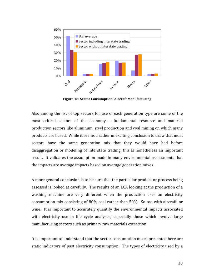
the top petroleum state. Aircraft manufacturing, the consumption mix of which is
shown Figure 16, has long made its home in hydro-heavy Washington and
California, and the disaggregated results show about 30% hydroelectric generation.
There are also more wineries in California than anywhere else in the country, and
California has a large amount of “Other” power; wineries are a top sector for use of
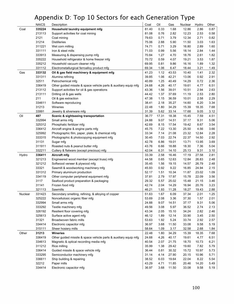
other generation types such as geothermal and wind. The top sectors for each type
of electricity are included in Appendix D.
Page 46
30
0%
10%
20%
30%
40%
50%
60%
Coal
Petroleum
Natura
l Gas
Nuclear
HydroOth
er
U.S. AverageSector including interstate tradingSector without interstate trading
Figure 16: Sector Consumption: Aircraft Manufacturing
Also among the list of top sectors for use of each generation type are some of the
most critical sectors of the economy – fundamental resource and material
production sectors like aluminum, steel production and coal mining on which many
products are based. While it seems a rather unexciting conclusion to draw that most
sectors have the same generation mix that they would have had before
disaggregation or modeling of interstate trading, this is nonetheless an important
result. It validates the assumption made in many environmental assessments that
the impacts are average impacts based on average generation mixes.
A more general conclusion is to be sure that the particular product or process being
assessed is looked at carefully. The results of an LCA looking at the production of a
washing machine are very different when the production uses an electricity
consumption mix consisting of 80% coal rather than 50%. So too with aircraft, or
wine. It is important to accurately quantify the environmental impacts associated
with electricity use in life cycle analyses, especially those which involve large
manufacturing sectors such as primary raw materials extraction.
It is important to understand that the sector consumption mixes presented here are
static indicators of past electricity consumption. The types of electricity used by a
Page 47
31
particular sector and the emissions associated with that use are based on a
hypothetical snapshot using data from 1997 and 2000. The model does not have
any inherent predictive ability beyond providing information upon which
assumptions can be based. Using it as a predictive model could produce misleading
or unwanted results. Nor does it allow for marginal changes due to demands for
different types of power.
Consider the case where a paper manufacturer has a facility located in Georgia. He
pays an average of 6.5 ¢/kWh for electricity to power his manufacturing processes.
He is looking for ways to reduce his expenses and therefore increase the
profitability of his paper production business. Since he purchases large amounts of
power along with his wood and water, a reduction in the amount spent on electricity
would certainly help.
Prices in Washington state are significantly lower for electricity. Anywhere from .5¢
to 3¢ per kilowatt hour less. Power generators in Washington produce almost ¾ of
their electricity from hydroelectric dams, and as a result they are able to sell at a
much lower cost than those generators that have to buy fuel. A move to a facility
near all this cheap hydro power might produce the sorts of cost savings and profit
increases the paper mill owner was looking for.
And this is likely true for individual facility owners: a move to an area with cheap
renewable electricity production will result in lower electricity costs. But as more
individuals make this choice, the model results will no longer show what’s going on
in the market.
Very little new hydroelectricity generation is being installed in the United States due
to the large ecological cost associated with dam and reservoir construction. And the
hydroelectric power currently being generated is sold as soon as it is produced
because it can be produced so cheaply. So, new capacity that is required to power
Page 48
32
facilities such as the relocated paper mills will not come from hydroelectric dams. It
is also not likely to come from nuclear or other renewable sources due to the high
prices of those types of facilities. Finally it is unlikely to come from coal generation
because coal-fired generators are poor peak producers – they can’t produce
electricity on short notice for high demand periods because of the time required to
ramp up and ramp down the facility. So the new generation is likely going to come
from natural gas fired power plants.
Increased demand in the state will result in one of four possible outcomes:
1. Increased production in the state from coal, gas or other renewable energy
sources
2. Increased production, and reduced export of power
3. Reduced electricity exports
4. Increased imports from another state
Now, as more individual entities make the choice to move to cheap – and carbon-
free – hydroelectric producing states, the power they are using will likely come from
more expensive fossil fuel fired plants. It is important to understand these small
changes at the margin might actually change the structure of the economy due to
changing supplies and demands, but this isn’t accounted for in the model. However,
input-output models are robust to small changes in demand – in this case, the
existing (static) amount of hydro power will be reallocated among all previous and
the new demands.
2.3 Comparing Results In order to compare a life-cycle analysis which uses an average mix to those using
consumption or generation profiles, a basic disaggregation of the power generation
and supply sector needs to be completed and put into an input-output framework.
This means splitting the existing Power Generation and Supply sector into six
separate sectors, one for each generation type discussed in this chapter. The
mechanics of disaggregation are discussed in detail in Chapter 3, and is the main
Page 49
33
focus of this dissertation, but for the purposes of this comparison, a much simpler
version is used. In this version, only the four most economically important sectors
are allocated to specific generation type: coal mining, oil and gas extraction, rail
transportation and pipeline transportation. The remaining sectors are allocated
based on kilowatt-hours generated and an average electricity price.
One important enhancement done here is that three complete sets of supply chains
are created for the other 490 sectors in the economy, and each one has different
values for their purchases from Power Generation & Supply.
1. Electricity treated as a single sector – this is the US average mix, and the
current method of dealing with electricity purchases
2. Six separate electricity purchases, with purchases based on the sector-
specific generation mix, ignoring trading
3. Six separate purchases, using a sector specific consumption mix, with trading
Once the new supply chains are complete, a total requirements matrix is created
according to the BEA process for building their input-output model from the
economic census77. Details on this process, and the MATLAB code used to
implement it are included later. A single emission factor, that for CO2, is used in this
analysis, for simplicity of comparison. Four scenarios were used to compare the
consumption and generation mixes to the average mix. To run these scenarios, the
amount specified is entered into the model as a final demand.
The first scenario models the purchase of a new 777 airliner from Boeing. This is
the purchase of the unit itself only, not the use of it, so there are no fuel costs. A new
777 costs about $220M according to Boeing, and assuming it costs Boeing about
70% of the price to make it, the construction is reflected as a $155M purchase in the
aircraft manufacturing sector, which is IO code 336411. We would expect that
because this industry had a very different profile from the US average, that its CO2
numbers would be lower as well.
Page 50
34
The second scenario looks at the purchase of a new domestic luxury sedan for
$50,000. Using the same cost/price assumption, this is modeled as a $35,000 final
demand from automobile manufacturing. The third scenario looks at $1 million
worth of coal from the coal mining sector, and finally, the fourth looks at $1 million
in retail purchases, which we would expect to have a mix very similar to the rest of
the United States.
For each scenario, the results show the tons of CO2 emitted due to total electricity
use over the life-cycle of the purchase specified above. The “Average” results shows
the carbon emitted with the US average mix – electricity is purchased from an
aggregated sector. The “Generation” and “Consumption” results are disaggregated
into six sectors, but of those six, only three – coal, petroleum and natural gas – had
direct carbon emissions.
-5,000
10,00015,00020,00025,00030,00035,00040,00045,000
Average Generation Consumption
Natural GasPetroleumCoal
Figure 17: CO2 (metric tons (MT)) from electricity used by Aircraft Manufacturing
In the first case, shown in Figure 17, comparing emissions from the purchase of the
777, we see that when looking at total emissions, there is not a significant change
from the average, in fact, only about a 2% and 1% reduction respectively for
generation and consumption. Notice that trading drives the number back up
Page 51
35
towards the average. This is because while aircraft manufacturers might be located
in the northwest, their suppliers are not. The direct purchase of power by the
aircraft manufacturing sector had lower carbon numbers – about a 5% reduction,
reflecting their location and different electricity profile.
-
100
200
300
400
500
600
700
Average Generation Consumption
Natural GasPetroleumCoal
Figure 18: CO2 (MT) from electricity used by Coal Mining
In Figure 18, we see something quite different from the coal mining purchase. The
electricity purchased by the coal mining sector and its suppliers is dominated by
coal-fired power, and that is reflected in a 20% increase in total carbon. The direct
purchase of power, shown in Figure 21, is even more different, almost a 40%
increase in carbon over the US average mix purchase. Again, the averaging effect of
interstate trading can be seen – the carbon emissions from the consumption mix are
closer to the average than the generation value.
Page 52
36
-
2
4
6
8
10
12
14
Average Generation Consumption
Natural GasPetroleumCoal
Figure 19: CO2 (MT) from electricity used by Automobile Manufacturing
The results for the automobile scenario are similar but not quite as dramatic, with a
7% increase in total carbon over the average mix shown in Figure 19. Like coal
mining, the direct numbers were higher than the total, with a 15% increase for the
generation mix and a 14% increase for the consumption mix. These numbers a
likely due to the presence of most domestic car production in the eastern United
States, from Michigan to the upper southern states like Tennessee, which are states
with lots of coal-fired power.
-
50
100
150
200
250
300
350
400
Average Generation Consumption
Natural GasPetroleumCoal
Figure 20: CO2 (MT) from electricity used by Retail
Page 53
37
Retail purchase results show in Figure 20 look like we would expect them to look –
very similar to the US average. It is interesting that there is any difference at all.
This might indicate that retail sales are not perfectly distributed across the country,
but in fact happen more where fossil fuel-fired power is available. These results are
also a good verification of the assumptions in general. A well dispersed sector that
we expected to have emissions close to the average, had results which were very
close.
-4%
0%
4%
8%
12%
16%
20%
Aircraft Mfct AutomobileMfct
Coal Mining Retail
GenerationConsumption
Figure 21: Percent difference of CO2 compared to US Average Mix
In Figure 21, the percent differences from average CO2 emissions from direct
electricity purchases by the sector of interest are shown. This is a summary chart,
not broken out by fuel type There are slight differences between consumption and
generation mixes, with consumption mixes always pushing the value towards the
average.
With these scenarios done, we wanted to look at how all the sectors in the economy
compared to each other in terms of CO2 emitted, for both the direct purchase of their
power mix, and total power purchases – that power purchased by all their suppliers.
Page 54
38
A loop was run through the model, plugging in $1 million of final demand for each
sector. The changes in direct and total CO2 from the carbon dioxide produced by
the US average mix are shown in Figure 22 and Figure 23.
-60% -45% -30% -15% 0% 15% 30% 45% 60%
Coal mining
Household laundry equipment mfct
Wineries
Household vacuum cleaner mfct
Household refrigerator & home freezer mfct
Distilleries
Small arms mfct
Measuring & dispensing pump mfct
Ferroalloy & related product mfct
Wet corn milling
Iron & steel mills
Burial casket mfct
Automobile & light truck mfct
Support activities for other mining
Other major household appliance mfct
Semiconductor mchnry mfct
Motor home mfct
Motor vehicle parts mfct
Aluminum sheet, plate, & foil mfct
Truck trailer mfct
Aircraft mfct
Electricity & signal testing instruments
Elevator & moving stairway mfct
Photographic & photocopying equipment mfct
Fluid power pump & motor mfct
Other engine equipment mfct
Sound recording industries
Guided missile & space vehicle mfct
Seafood product preparation & packaging
Industrial pattern mfct
Industrial truck, trailer, & stacker mfct
Cigarette mfct
Semiconductors & related device mfct
Figure 22: Change in CO2 emissions from direct purchase of electricity
Figure 22 shows the increase or decrease in CO2 emissions from the average mix for
the direct purchase of electricity from the sector specified. The error bars show
Page 55
39
difference between consumption and generation mix results, with the bar being the
average between the two values. One interesting thing to note is the number of
important raw material extraction and processing industries with very different
mixes. Coal mining, iron and steel mills, automobile and aircraft manufacturing,
semiconductors and aluminum are all very different from the average mix.
Also apparent is the “California effect” where California’s distinct mix is reflected in
industries traditionally associated with California, like wineries, semiconductors
and missile and rocket manufacturing. Generally these sectors have a large spread
between their consumption and generation bars as well – once California is
penalized with coal imports, the carbon numbers for those sectors move back
towards the average.
Page 56
40
0% 15% 30% 45%
Coal miningFerroalloy & related product mfct
Wet corn millingIron & steel mills
Iron, steel pipe & tube from steelBurial casket mfct
Household laundry equipment mfctOther nonmetallic mineral mining
Iron ore miningFerrous metal foundaries
Custom roll formingRolled steel shape mfct
Steel wire drawingFluid power pump & motor mfct
Support activities for other miningElevator & moving stairway mfct
Lime mfctNonclay refractory mfct
Motor vehicle parts mfctHousehold vacuum cleaner mfct
Mining machinery & equipment mfctFarm machinery & equipment mfct
Industrial pattern mfctPrefab metal buildings & components
Other engine equipment mfctOther ordnance & accessories mfct
Industrial truck, trailer, & stacker mfctIron & steel forging
Mineral wool mfctPlate work mfct
Ground or treated minerals & earths mfctSpecial tool, die, jig, & fixture mfct
Copper, nickel, lead, and zinc mining
Figure 23: Change in CO2 emissions from total electricity purchases
Shown in Figure 23 are the changes in carbon from the average mix for total
electricity purchases. In total purchases, the “California effect” disappears, since the
suppliers for California’s industries look much more like the rest of the country than
they do like California. But once again, the sectors present here are very important
sectors to the US economy – major material extraction and processing sectors and
large manufacturing sectors.
Page 57
41
Also, once the impact of all suppliers is included, the differences are much smaller –
supply chains change the power mix and make it more like the average. For direct
CO2, over 30 sectors had more than a 15% difference, and the largest difference was
over 50%. In the total results, only about 20 sectors were greater than 15%, and not
by much. The largest difference was just over 40%.
The main conclusion of this analysis is that disaggregation of the electricity sector
matters. While many sectors in the economy have similar mixes and similar
emissions to the US average mix – the aggregated version of the power generation
sector – there are sectors which are different and they are important sectors.
This conclusion is not just important in that it justifies the work shown later, but
because it is important that LCA practitioners of all types are aware that for many
sectors which they are interested in, the mix of electricity used is important data to
gather. Even if the results are simply used as a comparison – to prove that the
average mix or emissions is a good assumption – disaggregated electricity matters
for accurate environmental inventories
Page 58
42
3 Building a disaggregated electricity model At a high level, this work involves adding detail to the Power Generation & Supply
(PG&S) sector of a 491-sector model of the US economy to allow for more detailed
economic and environmental analysis of the electricity industry. It can be thought
of as splitting up, or disaggregating, this sector into between 6 and 24-plus
additional sectors, each representing a specific portion of the electricity industry;
for instance, a sector for Pulverized Coal Generation Operations and Maintenance, or
Wind Turbine Construction, as seen in Figure 24. Included with each of these
disaggregated sectors will be a supply chain – what the sector purchased from the
other 500 sectors in order to produce its output (i.e. a power plant, or a kWh of
electricity) – and a set of emission factors which will allow calculation of the
environmental impact of the sector’s output. When all the new sectors are inserted
into an existing economic input-output framework, we can build future generation
scenarios – each with a specific mix of generation types and investment in future
technologies – and we can look at the economic and environmental results which
include not only the top-level emissions, but the impacts from the entire supply
chain.
Figure 24: Disaggregating the Power Generation & Supply Sector
Page 59
43
The following chapter will discuss building the disaggregated electricity sector
model including major inputs and outputs, data sources, and the methods used.
3.1 Model Inputs The following section details the inputs required for the model to run. There are
two important things to note about the inputs for the model. The first is that
wherever possible, ranges are used for these inputs rather than point estimates.
This enables a range of outputs to be reported, thereby dealing explicitly with the
inherent uncertainty of parameter value choice. In some cases, the range will be the
maximum and minimum values found or calculated; in other cases, it will be a set
percentage above and below an average or median value found or calculated.
The mechanics of how the output range is calculated is less than ideal: a version of
the model is calculated using the low end of all ranges, and a version is run with the
high end of all ranges. The output of those two runs is used as the high and low end
of the output range. This method decreases the amount of time required to
complete a scenario, and in a linear model, it is a good approximation of output
range. In a non-linear model, we would need to be worried about non-linear
response to changes in input parameters.
The second important thing to realize about the ranges collected for input values is
that they are ranges on averages. It might help to think of them as the first standard
deviation on a mean: it captures a lot of the variability associated with a parameter,
but not the extremes – although it is certainly influenced by the presence and
magnitude of those extremes. Although the electricity sector is being disaggregated
into major generation types, there is still a significant amount of aggregation that is
happening.
For instance, all pulverized coal plants, all coal types, and all customers are being
aggregated together under the generic sector “Coal-fired Operations &
Page 60
44
Maintenance”. The values of cost per kilowatt-hour, or tons of carbon per kilowatt-
hour, etc. need to be averages for all of those plants and coal types. Collecting and
using data on the worst performing coal power plant, and the newest, most
sophisticated plant as the low and high points for a range would mean that we
expect that on average all plants could perform at that data point, and we know that
this is not true. This makes the data collection and uncertainty analysis more
complicated.
In practice, when these ranges are used, care is taken to make sure they are used
correctly. Although an input parameter’s “low” range value may be below the
average, its influence may push the output result higher. In this text, the labels
“low” and “high” refer to standard numerical ordering, though in the model the use
may be opposite – a lower value affects the upper bound.
3.1.1 Supply Chains
In order to build a new input-output model, we need to modify the components that
go into making it, and the first of these is the use table, which can be thought of as
the supply chains for all the industrial sectors in the economy. So, for every
disaggregated sector to model, a listing of the commodities and corresponding
dollar values (or the relative proportions of a dollar) needed to produce the output
of the new sector must be created. This is true for both the Operations &
Maintenance and Construction sectors, although the construction sectors will not be
inserted into the final model of the economy. This point will be explained in more
detail in 3.4.3.
In addition to the supply chains for each new sector, the existing supply chains for
every other sector in the model which uses electricity needs to be modified as well.
Where in the aggregated model, each of these sectors would have purchased
electricity from a single sector, Power Generation & Supply, now they purchase from
a mix of generation sectors. This mix can be determined in two ways: first, an
average mix can be used, based on the assumed overall mix of generation types,
Page 61
45
second, a specific sector mix based on the work shown in Chapter 2. Note that these
sector specific mixes will only be used if the scenario being run includes all the
generation types used in that analysis. For instance, if a sector mix includes use of
natural gas, but there are no natural gas plants included in the scenario, then a
different mix assumption will need to be used.
3.1.2 Sector Output
The make table, which is a matrix of commodities produced by industries, needs to
be created for the disaggregated power generation sectors. In the existing make
table, the entry is more complex than a 1-to-1 industry-to-commodity relationship.
In addition to power, the Power Generation & Supply provided other utility
commodities in the form of delivered steam heat from combined heat and power
(CHP) units. Other industries make the commodity “power generation” as well. The
dollar values and commodities need to be put into proper disaggregated sector
make entry.
3.1.3 Emission Factors
In order to generate environmental output from an economic model, the data which
is normally available in units of mass per unit output needs to be converted to mass
per dollar output. The emissions tracked in this model will be CO2 and the major
criteria pollutants SOX and NOX.
For the most part, the emission factors are adapted the from the Environmental
Protection Agency’s eGRID model, which in turn are based on the AP-42 emission
factor data source.39
3.1.4 Electricity Costs
To connect the physical quantities normally associated with electricity such as
kilowatt-hours and tons of emissions per kilowatt-hour with the dollars in the
input-output model it is important to have good estimates of the costs per kilowatt-
hour. These are not retail prices, levelized or overnight costs which include the cost
Page 62
46
of capital, but the pure cost of operation. The cost of operation is needed for each
generation type.
We are making the assumption that all capital investment in the power generation
sector, such as new plant construction, will happen outside the model of the
economy built with the make and use tables. If the supply chains for operations and
construction were combined, then we could use levelized capital costs rather than
operations costs.
3.1.5 Final Demand
In order to generate output from the model, a final demand is needed. If the goal of
the analysis is the life-cycle assessment of some other sector with disaggregated
electricity output, then the final demand would be placed in that sector. If the
analysis is more complex electricity scenario, the final demands need to be put into
the a mix of disaggregated electricity sectors – both operations and whatever
construction occurs in the scenario. If the scenario is based on a demand in
kilowatt-hours, then those kilowatt-hours need to be converted to a final demand
using the electricity prices discussed above.
3.1.6 Input Summary
• Set of generation operation sectors
o Each with an emission vector, a supply chain vector, and cost/kWh
• Set of plant construction sectors
o With emission vector
o Supply chain vector in $ or relative $/kW
• Sector-by-sector consumption mixes (US average or spatially specific)
• Scenario annual generation mix (%)
• Scenario annual construction mix (%)
• Annual electricity demand (kWh)
• Annual construction investment ($)
Page 63
47
3.2 Model Outputs The final outputs of the model are economic and environmental results for every
sector in the economy. For each of these, results will be given as direct, indirect and
total. There are also two intermediate outputs, an updated total requirements
matrix of inter-industry purchases, and an updated emissions vector. The original
1997 BEA-supplied sector is 491x491 – the new matrix will remove the original
PG&S sector and add n more sectors for a 490+n x 490+n matrix depending on how
many sectors are being modeled.
3.3 Data Sources There are four major types of data sources used in collecting information for the
various inputs and scenarios:
1. Government data (Bureau of Economic Analysis, DoE Energy Information
Administration, Environmental Protection Agency, etc.)
This includes industry data collected by these government agencies, and data
synthesized from collected data. For instance, the EIA publishes data
collected from the industry and also results from the NEMS model.19 The
EPA reports plant-by-plant emissions through eGRID, and also national
average emission factors synthesized from those numbers.
The BEA’s input-output model is the synthesis of the economic census. While
there is uncertainty in these numbers due to collection methods,
assumptions, etc., use of these data sources is widespread, accepted and
justifiable. This data is available for every five years (1992, 1997, 2002),
with a three to four year lag. The 2002 data should be available in late 2006.
2. Literature sources
Although many sources in literature are papers synthesizing government
data mentioned above, there is a still quite a bit of unique, in-depth analysis
being done. While detailed, numbers gathered from these sources do not
always have clear assumptions spelled out, and sources of uncertainty are
sometimes not specified. Further, the data is rarely in a form that is directly
Page 64
48
applicable, so further assumptions are needed. Where appropriate, data
gathered from literature sources is noted and referenced.
3. Other models
Another form of data synthesis, energy or electricity models provide another
source of input values. The IECM, or Integrated Environmental Control
Model, is a probabilistic tool built at Carnegie Mellon to evaluate control
technologies for coal-fired and natural gas power plants, including various
forms of carbon control. In general, the information that IECM provides is
too specific for the data collection needs here, but it is possible to simulate a
“typical” or “average” power plant. 78,79 The existing version of the EIO-LCA
model provides emissions and environmental data for the other 490 sectors
in the model, and other work happening with the model provides data about
the construction sector.80
4. Industry
Because this is, at its base, an economic model, getting real world data from
the electricity industry would be ideal. However, the information we are
looking for is generally considered confidential, since we want to know what
they spend their money on and what it costs them to produce their product.
However, the federal government requires that utilities make some of this
information publicly available in a standardized format to FERC, the Federal
Energy Regulatory Commission, through the Form 1, the Annual Report of
Major Electric Utilities. The now partially deregulated industry is actively
fighting to have the financial reporting requirement removed, or at least
made completely confidential.81
There are several problems with the data available in the Form 1. The first is
that the data is hard to get to – there is no editable, searchable database to
access the data through. Data in this form would be much more useful to the
public. The second, and more important, problem is that the while the data is
required by Federal Code 18 to conform to a Unified System of Accounts,
Page 65
49
there is variability in the way different utilities report the data, due to
different accounting practices, the size of the utility, and the types and age of
the generation assets the utility operates.81 Lastly, the data in some cases is
very general – like fuel purchases, which could be easily mapped to a sector
like “coal mining” or “oil and gas extraction”, or very detailed, like the
purchase of a specific piece of environmental control equipment for a
particular power plant. It is difficult to ascertain what the equipment is for
and what sector the purchase should be mapped into.
Finally, not all purchase data provided by the utilities in the Form 1 – with
the exception of fuel – are attributed to a particular plant or fuel type.
Although we could determine generation assets for a particular utility, we
would still need to allocate the purchases in the Form to their assets in some
way.
In the 2004 form for Southern Company, on page 204, line 14 specifies they
spent $926,000 on “Misc. Power Equipment.” Page 204, line 14 is in the
“Steam Production Plant” section, but the fuel type of those plants is not
specified.82 Although this is a very definitive piece of data from industry, it is
indicative of the sorts of problems Form 1 data presented. We know that
Southern has a large variety of generation assets, and it is not clear what type
of plant this equipment went towards. It is also unclear, which commodity
sector we should reflect this purchase in. There are several commodities
which list power equipment of various types. Finally, we don’t know if that
purchase is typical for the industry as a whole, or for 2004.
3.4 Building the Model To begin the process of building the disaggregated model, a decision needed to be
made about what level of disaggregation, and, conversely, aggregation, was
appropriate for the Power Generation & Supply sector. Past disaggregation work,
discussed in Chapter 2, was limited to six operations sectors, split up by aggregated
Page 66
50
fuel type, i.e. “coal” as opposed to anthracite, bituminous, sub-bituminous coal.
These sectors were given generic, sequential Input-Output codes: 221101, 221102,
etc. Although this is an excellent rough cut, as it allows for discernment of the major
environmental differences, analysis of future generation scenarios requires a
greater ability to focus on renewable generation. The North American Industry
Classification System (NAICS) breaks the industry down into only five 6-digit
sectors, shown in Table 4. Six digit codes are needed to represent sectors in EIO-
LCA and the new electricity-focused model.
Table 4: Original NAICS Sector 2211 Definition83
Code NAICS Sector Definition 2211 Electric Power Generation, Transmission and Distribution 22111 Electric Power Generation 221111 Hydroelectric Power Generation 221112 Fossil Fuel Electric Power Generation 221113 Nuclear Electric Power Generation 221119 Other Electric Power Generation 22112 Electric Power Transmission, Control, and Distribution 221121 Electric Bulk Power Transmission and Control 221122 Electric Power Distribution
Table 5 shows selected six digit codes for construction sectors along with their
parent sectors. Here, there are only three six digit codes to represent all the
different types of construction that happens in the electricity sector, with
transmission and distribution being under 234920, hydroelectric construction
under 234990 and all other types of power plants under 234930.
Table 5: Selected Original NAICS Sector 23 Definition83
Code NAICS Sector Definition
23 Construction 234 Heavy Construction 2349 Other Heavy Construction 23492 Power and Communication Transmission Line Construction 234920 Power and Communication Transmission Line Construction 23493 Industrial Non-building Structure Construction 234930 Industrial Non-building Structure Construction 23499 All Other Heavy Construction 234990 All Other Heavy Construction
Page 67
51
It is clear from these limited sector definitions that to have reasonable granularity in
the updated model, that new – though not official – sector definitions will be needed.
In Table 6, a new sector definition scheme is laid out, which allows for the necessary
detail. Remember, though, that there is still significant aggregation happening at
this level. Under the “Pulverized Coal” plants sector, all different coal types are
grouped together, as are different plant designs and levels of environmental control.
Under “Nuclear”, PWR and BWR plants are grouped together, as are advanced plants
like the AP-1000 or fluidized pebble-bed reactors. All classes and designs of wind
turbines are under a single “Wind” sector, and both single and combined-cycle
natural gas plants are under “Natural Gas.”
Table 6: PG&S O&M Sector Redefinitions Code NAICS Sector Definition
2211 Power Generation and Supply 22111 Fossil Fuel Power Generation 221111 Pulverized Coal 221112 IGCC 221113 Natural Gas 221114 Petroleum 22112 Renewable Power Generation 221121 Hydroelectric 221122 Solar 221123 Wind 221124 Geothermal 221125 Biomass 22113 Other Power Generation 221131 Nuclear 22114 Power Supply 221141 Transmission 221142 Distribution
For construction, a similar redefinition is necessary, while at the same time making
sure that data isn’t currently being collected and reported by the BEA in the sectors
being redefined, as well as using existing definitions if appropriate.
Table 7: PG&S Construction Sector Redefinitions
Code NAICS Sector Definition
Page 68
52
23 Construction 234 Heavy Construction 2349 Other Heavy Construction 23492 Power Transmission Line Construction 234920 Power Transmission Line Construction 23493 Power Plant Construction 234931 Pulverized Coal Power Plant Construction 234932 IGCC Construction 234933 Natural Gas & Petroleum Plant Construction 234934 Hydroelectric Power Plant Construction 234935 Nuclear Power Plant Construction 234936 Wind Turbine Construction 234937 Solar Construction 234938 Biomass Construction 234939 Geothermal Construction
Despite the redefinitions, these are obviously not comprehensive lists of generation
technologies – either current or future – or a full set of construction work that could
take place in the industry. Because from the outset, it was known that no
disaggregation could ever be complete, the framework is open and infinitely
expandable. If the goal was to model and compare the construction and operation of
two sub-bituminous pulverized coal plants, one with minimum environmental
controls, and another with best available technology, sectors could be created to do
the job, if the data was available. Likewise, if you wanted to compare the Hoover
Dam to the Grand Cooley Dam over their lifetimes, sector supply chains and
emissions factors could be created to do that as well if data could be collected.
3.4.1 Estimating Electricity Costs
Although there are many alternative sources to choose from84, we chose to use
Department of Energy information to create our estimates for electricity costs.
Coming up with the price of electricity is generally a very complicated process that
must take into consideration the spot prices of fuels, depreciating capital costs, taxes
and regulatory environment, transmission infrastructure, type of consumer, etc.85
Coming up with operating costs, by contrast is a much easier exercise. These costs,
in dollars per kilowatt-hour ($/kWh), include annual fixed operations &
Page 69
53
maintenance costs which are dependent on plant size (capacity), and variable O&M
costs, like fuel, which are dependent on output generated. To convert fixed costs to
output-based costs, we used ranges of capacity factors from the National Renewable
Energy Laboratory.86
Recall that these costs do not include any capital costs. These are not busbar, but
operations costs only. The reasoning behind using operations costs only is
explained further in section 3.4.3. Department of Energy estimates of various fossil
fuel costs are shown in Figure 25, in real dollar terms. Coal prices are increasing,
but look stable relative to petroleum (No. 2 fuel oil & diesel) and natural gas prices
which have quadrupled since 1998.
0
1
2
3
4
5
6
7
8
9
1997 1998 1999 2000 2001 2002 2003 2004 2005
$/M
Btu
Coal Petroleum Natural Gas
Figure 25: Fossilfuel prices paid by Electricity Generators1
In the estimate of electricity cost shown in Figure 26, an average is shown in the
column graph, with variability in fuel price over an 8-year span, in capacity factor
and heat rate accounted for by the error bars. For the fossil fuel generation types,
the variability is almost entirely due to fuel price since there is little uncertainty
associated with the technology associated with those plants. For generation types
to the right of Figure 26, the variability has more to do with differences in
Page 70
54
technology implementations and operations reliability. In this case, costs are in
nominal 1997 dollars to match the rest of the input-output economic data.
$0.00
$0.01
$0.02
$0.03
$0.04
$0.05
$0.06
Coal
IGCC
Nat
. Gas
Petr
oleu
m
Nuc
lear
Hyd
roel
ectr
ic
Geo
ther
mal
Win
d
Sola
r PV
Sola
r T
herm
.
Land
fill
Gas
Bio
mas
s
$(19
97)/
kWh
Fixed O&M
Variable O&M
Figure 26: Electricity O&M Prices by Generation Type7,8,8693
The same information is included in table form below. These are intended to be
average electricity costs taking into account a wide range of technologies and fuel
prices. The estimates are important, though, because they will be used for the
default allocation method which will be shown below, and also for the creation of
dollar-based emission factors. However, these prices, could be made much more
specific – to be representative of a specific year or technology type, and those
changes will be made for some of the scenarios.
Table 8: Electricity O&M prices by Generation type ($1997/kWh) 7,8,8693
Technology Average High Low
Coal $ 0.017 $ 0.018 $ 0.015 IGCC $ 0.014 $ 0.017 $ 0.012 Natural Gas $ 0.031 $ 0.053 $ 0.018 Petroleum $ 0.021 $ 0.030 $ 0.015 Nuclear $ 0.007 $ 0.009 $ 0.006 Hydroelectric $ 0.009 $ 0.014 $ 0.006 Geothermal $ 0.010 $ 0.015 $ 0.007 Wind $ 0.007 $ 0.012 $ 0.005 Solar PV $ 0.006 $ 0.010 $ 0.002 Solar Thermal $ 0.013 $ 0.023 $ 0.006
Page 71
55
Landfill Gas $ 0.013 $ 0.017 $ 0.010 Biomass $ 0.008 $ 0.009 $ 0.007
3.4.2 Creating Operations Supply Chains & Industrial Output
Originally, when the idea of disaggregating the electricity sector came up, the
intention was to build new supply chains from scratch. A coal-fired power plant, for
instance, must purchase a certain amount of coal (from the coal mining sector), the
transportation happens by rail and barge. Additionally, it requires ammonia for NOx
reduction with SCR and calcium for sulfur emissions control with FGD. They utilities
probably have lawyers and consultants. It seemed that the supply chain would be
relatively small and easy to create.
However, the initial investigation showed that the BEA supply chain (in the form of
a use table) for the Power Generation and Supply sector (IO/NAICS code 221100)
included purchases of 183 separate commodities, which was far more than came
from the original estimation. Table 9 shows the top 17 sectors of the BEA supplied
use table in producer prices. There are some obvious sectors near the top: coal
mining and rail transportation supplying coal to coal-fired power plants, and oil and
gas extraction and pipeline transpiration supplying natural gas and petroleum fired
plants. There are some surprises, however, like the large maintenance and repair
contribution, money spent on real estate, or on courier and messenger services. The
power of the input-output type of life-cycle assessment is the eradication of the
boundary issue, and shortening these chains might reintroduce some of those
problems.
Table 9: 1997 Benchmark use table for PG&S3
Sector Use Value ($M) % of Total
Coal mining $15,098 18.9% Oil and gas extraction $14,905 18.6% Pipeline transportation $6,669 8.3% Rail transportation $5,844 7.3% Other maintenance and repair construction $3,389 4.2% Legal services $3,232 4.0% Petroleum refineries $2,151 2.7%
Page 72
56
Monetary authorities and depository credit $1,855 2.3% Wholesale trade $1,754 2.2% Advertising and related services $1,749 2.2% Food services and drinking places $1,660 2.1% Real estate $1,582 2.0% Truck transportation $860 1.1% Couriers and messengers $626 0.8% Water transportation $597 0.7% Wiring device manufacturing $536 0.7% Switchgear and switchboard apparatus $529 0.7%
Although the supply chain is long and contains some surprises, it is extraordinarily
top heavy, with most of the money being spent on the top commodities, and the
contribution of commodities lower in the chain being very small, percentage-wise.
The top 12 sectors accounted for 75% of the economic value, the top 35 accounted
for 90%. Put another way, the bottom 146 sectors have only 10% of the economic
value of the supply chain. Additionally, most of the sectors at the top are the most
environmentally important, as well, although additively service-related
commodities have a large impact as well.94 And, some assumptions can be made
about these top sectors. The $15 billion spent on coal mining was a purchase from
the coal-fired generators. This is a direct-use value, and it makes no sense for coal
to be purchased by any other generator at any point in their supply chain.
Table 10: Assumptionbased allocation across generation types
Commodity PG&S Supply Chain Value ($M)
Coal Allocation
Petroleum Allocation
Natural Gas Allocation
Coal mining $ 15,098 100% 0% 0% Oil and gas extraction $ 14,905 0% 9% 91% Pipeline transportation $6,669 0% 9% 91% Rail transportation $5,844 100% 0% 0% Petroleum refineries $2,151 0% 9% 91% Water transportation $597 100% 0% 0%
Table 10 shows some of the other important sectors about which we have made
assumptions. There are other sectors in the supply chain about which we can make
these sorts of assumptions, but the economic impact of those decisions is limited
Page 73
57
because of the small relative contribution of the commodity to the overall supply
chain. For sectors like “Oil and gas extraction” which have a 9%/91% allocation, it
is assumed that all use of that sector comes from petroleum and natural gas
generation, and the money is spent in proportion to the weighted kilowatt-hours
produced, explained below.
The other sectors, about which there is limited or no information, are a bit more
difficult. Rather than introduce additional uncertainty by using external sources or
attempting to justify assumptions, a default allocation method is used. Originally,
the idea was to use the current US generation mix as a means of allocating these
dollars. So 49.9% of the money spent on a commodity would be allocated to coal-
fired generators, since that percentage of kilowatt-hours were generated by those
plants. However, since this is an economic model, the allocation should probably be
based on how the dollars were spent to generate output, not the output itself.
0% 25% 50% 75% 100%
High
Low
Average
Generation
Coal Nuclear Natural Gas Hydro PetroleumBiomass Geothermal Wind Other Solar
Figure 27: Pricedbased Default Allocation
Page 74
58
Figure 27 shows the US average generation mix, and then the price-based “mix”
using average, high and low price per kilowatt-hour estimates. There are dramatic
differences in how the money in the supply chain gets allocated. Coal-fired
electricity (49.9% of generation) goes from an average 48% to as high as 60% when
coal prices are low to 40% when coal prices are high. Natural gas is only 19% of the
generation mix, but can account for as much as 44% of the money spent if natural
gas prices are high enough.
Table 11: Pricedbased Default Allocation
Technology Generation Average High Low
Coal 49.9% 48.9% 39.9% 58.2% Nuclear 19.3% 8.2% 7.5% 8.6% Natural Gas 19.0% 34.8% 43.8% 25.7% Hydro 6.4% 3.4% 3.8% 2.8% Petroleum 3.0% 3.7% 4.0% 3.5% Biomass 1.5% 0.7% 0.6% 0.9% Geothermal 0.4% 0.2% 0.2% 0.2% Wind 0.4% 0.2% 0.2% 0.1% Other 0.1% 0.1% 0.1% 0.0% Solar 0.0% 0.0% 0.0% 0.0%
So, all other sectors are allocated based on this assumption that the commodities in
the supply chain were used in proportion to the amount of output generated. This
may not be strictly true – in fact it most certainly isn’t. Nuclear plants may spend
more on safety equipment, and coal plants may spend more on environmental
control equipment, but the output proportionality assumption is a good first order
estimate for most sectors.
But before a final allocation is settled on, spending on transmission and distribution
needs to be taken into account, since those sectors, or functions of the industry, will
be part of the disaggregation. Adjusted for inflation, spending on distribution has
stayed relatively constant over since 1994, at around $4.5-5 billion annually.
Page 75
59
Transmission spending has increased in recent years, from a low of about $2.4
billion in 1996 to over $5 billion in 2005.
$-
$1
$2
$3
$4
$5
$6
$7
$8
1994 1995 1996 1997 1998 1999 2000 2001 2002 2003 2004 2005
$(19
97) B
illio
ns
0%
1%
2%
3%
4%
5%Transmission Distribution
Figure 28: T&D expenditures, and as percent total utility expenditures1
The spending on both of these areas is rising as a percentage of total industry
expenditures, from around 3% to about 4.5%.1 Since our sector of interest includes
both generation and supply, the list of commodities used should have a percentage
allocated to the supply of the electricity. Figure 28 shows this information – by
contrast, spending on biomass, geothermal, wind and solar generation combined
was less than the amount spent on transmission and distribution.
Investment in transmission and distribution has been over $13 billion a year since
1975, and in the last ten years has been increasing each year, faster than the
increase in electricity demand, so this percentage will increase.
Page 76
60
$-
$3
$6
$9
$12
$15
1975 1978 1981 1984 1987 1990 1993 1996 1999 2002 2005
TransmissionDistribution
Figure 29: Transmission and distribution investment 19902005 ($B, 2005)95
The amounts shown in Figure 28 are combined with the allocations for generation
only created above, and the results are shown in Table 12. These results are for the
average case, although a range of value was generated and different allocations
created based on them. Notice that relative to the generation-only allocations
shown in Table 11, the percentages for each generation type are lower, since about
4% of spending overall is now allocated to transmission and distribution. So, of the
money spent by the electricity industry, about 4% was spent on supply, not
generation. So the weighted kWhs are now normalized across the remaining 96%.
Table 12: Default allocation, with transmission and distribution accounted for
Technology Average
Coal 46.88%Nuclear 7.83%Natural Gas 33.35%Hydro 3.26%Petroleum 3.51%Biomass 0.68%Geothermal 0.21%Wind 0.15%Other 0.05%Solar 0.01%Transmission 1.95%Distribution 2.13%
Page 77
61
This allocation, along with any generation-specific assumptions discussed above, are
used to build the operations and maintenance supply chains. Note that in 1997, the
Power Generation & Supply use table included $20.7 million in purchases from
itself. It is not clear if this is power purchased by utilities to make up for supply
short falls, or if this is power used on site to power various systems. The
assumption used for this analysis is that a generation type will purchase from a
similar generation type, so that all power purchased by a nuclear generator will be
generated by nuclear, and some will be used for power supply. This allocation is
shown in Table 13. It shows the portion of the $20.7 million spent by the sector on
the left on the sector across the top. Notice that each sector purchases some power
supply as well.
Table 13: Use table PG&S intersection allocation ($M)
221111 Coal
221114 Petrol.
221113 Nat. Gas
221131 Nuclear
221121 Hydro
221125 Biomass
221124 Geoth.
221123 Wind
221122 Solar
221141 Trans.
221142 Dist.
221111 9.71 0.20 0.22 221114 0.73 0.01 0.02 221113 6.91 0.14 0.15 221131 1.62 0.03 0.04 221121 0.67 0.01 0.02 221125 0.14 0.00 0.00 221124 0.04 0.00 0.00 221123 0.03 0.00 0.00 221122 0.00 0.00 0.00
In addition to supply chains, there are also outputs, or make table entries to be
allocated. Table 14 shows the sectors (other than Power Generation & Supply – that
entry is an intersection similar to the use intersection shown in Table 13) which
produced the commodity “Power Generation & Supply”. These are sectors which in
the course of producing their other output produce some power to sell – or
purchase some power and then resell it, like a local cooperative utility. It was
assumed that the power produced here would be similar to the average generation
mix since no better information was available. A case could be made for cooperative
utilities having a different average – more hydroelectric plants might be
cooperatively owned and operated because of the other benefits provided by dams,
but the analysis was not done to assess this. The framework is flexible to allow for
those sorts of additions.
Page 78
62
Table 14: Output of industries producing commodity “PG&S”
in $millions 221111
Coal 221114 Petrol.
221113 Nat. Gas
221131 Nuclear
221121 Hydro
221125 Biomass
221124 Geoth.
221123 Wind
221122 Solar
S00202 Local Utilities
10,396 778 7,395 1,737 723 150 47 33 2
S00101 Federal Utilities
3,896 292 2,772 651 271 56 18 12 1
3221A0 Paper Mills
121 9 86 20 8 2 1 0 0
S00203 Other local Gvmt
3 0 2 1 0 0 0 0 0
Power Generation & Supply, in addition to making the commodity “Power
Generation & Supply”, produces other types of commodities such as “Natural Gas
Distribution”. This production was allocated in a similar fashion to the allocation
done in Table 13. The PG&S – PG&S intersection was treated the same way. Again,
no clear information was available about which types of generation were producing
these other outputs, so a default allocation was used.
An example of a complete supply chain for one of the disaggregated sectors is
included in Appendix K.
3.4.3 Creating Construction Supply Chains
The construction sectors in EIO-LCA are a known problem area due to double
counting of on-site emissions and fuel purchases, and poor reporting from an
industry with many small businesses, and are a field of study by themselves.80,96 As
such, the supply chains for the construction sectors are treated slightly differently.
Initially, the plan was for the construction use tables to be included in the total
requirements matrix along with the operations and maintenance sectors. Some
form of allocation would occur to form each of those supply chains. However,
several things became obvious over the course of the research which led to the
construction supply chains being handled differently.
First, there are only two constructions sectors represented in the 1997 Power
Generation & Supply commodity use table. Table 15 shows those commodities and
Page 79
63
the value of the purchase by the power generation sector, the total purchases of
those same commodities by all other sectors. Although 19% is a significant amount
of commodity 230340, it is important to look at that purchase in the context of the
rest of the construction industry.
Table 15: Construction sectors in 1997 PG&S Use table, in $ billions3
Sector Description PG&S Use Total Use PG&S %
230320 Maintenance & repair of nonresidential buildings $111 $56,012 0.2%230340 Other maintenance & repair construction $3,389 $17,833 19.0%
Sector 230320 is only 7.4% of the total construction sector, so 0.2% of that is about
0.015% of the total, and sector 230340 is only 2.4% of the total industry, so 19% of
that is only 0.449%. Together, the PG&S purchase of construction and maintenance
is only 0.464% of the total industry purchases, a pretty small fraction.
-5%
0%
5%
10%
15%
20%
25%
1995
1996
1997
1998
1999
2000
2001
2002
2003
2004
2005
2006
2007
2008
2009
2010
CoalNatural GasNuclearRenewables
Figure 30: U.S. new electric generating capacity by fuel type1
In order to confirm that little construction happened in 1997, we can look at the
kilowatts of capacity added at that time. Figure 30 shows the percent of kilowatts of
new capacity added annually between 1995 and planned expansion to 2010, broken
down by generation type. It can be seen that in 1997, there is little or no additions
to capacity. Natural gas prices would reach their lowest point in 1998, and there
Page 80
64
would be a huge spike in capacity three years later when plants built because of
those low prices started to come online. But in 1997, the year represented in the
input-output table used for this model, there is virtually no construction. Certainly,
if there was any new construction in that year, it is not representative of expansion
in the industry in general overall.
In some ways, this year of relative inactivity in the electricity industry is a benefit,
since it allows the 1997 use table to be considered an exclusively operations and
maintenance supply chain.
However, it does mean that supply chains for construction of new power plants
need to be created from scratch. But when it comes to creating those supply chains,
a similar problem to the operations and maintenance sectors is found – while it is
possible to come up with a list of 20 or so major material inputs to the construction
of a power plant, the average supply chain for a construction sector provided by the
BEA includes over 200 commodity purchases.3 Table 16 shows several heavy
construction supply chains from the 1997 BEA input-output model. Notice that both
services, such as architects, and materials, such as concrete, are included in the
supply chain.
Table 16: Selected 1997 heavy construction sector supply chains, in billions3
Sector Description 230210 230220 230230 230240 230250
V00100 Compensation of employees, "Labor" $13,131 $82,551 $17,245 $6,231 $41,304
541300 Architectural & engineering services $1,525 $16,043 $2,084 $1,513 $8,865
V00300 Other value added $611 $6,994 $2,636 $455 $4,402
4A0000 Retail trade $300 $8,917 $646 $272 $1,793
420000 Wholesale trade $929 $5,103 $985 $577 $2,318
332312 Fabricated structural metal mfct $129 $2,852 $660 $231 $1,556
532400 Machinery & equipment rental & leasing $299 $1,642 $1,240 $467 $1,780
324110 Petroleum refineries $237 $1,738 $1,404 $304 $1,290
32619A Plastics plumbing fixtures $296 $2,451 $489 $154 $1,081
484000 Truck transportation $315 $1,814 $1,114 $341 $633
335120 Lighting fixture mfct $961 $2,508 $209 $86 $431
327320 Ready-mix concrete mfct $222 $1,507 $1,454 $97 $743
Page 81
65
In order to maintain the completeness of the service sectors included in these
supply chains but have materials specific to each power plant type, a hybrid
approach will be used. First, an “average” heavy commercial/industrial
construction sector will be created by averaging the dollar amounts spent in the
construction sectors shown in Table 16. Then, materials commodities will be cut
from that supply chain, leaving a service-only supply chain for a heavy construction
sector. These supply chain will then be used as a “template” for the creation of
generation-type specific construction supply chains which will include materials for
the construction of a typical plant of that type.
The template supply chain includes purchases from 120 commodities, which mostly
represent services. Because more materials sectors were cut out from the template
than will likely be replaced by our researched material supply chains, there will
likely be some components missing from the power plants purchased using this
model.
Construction material commodity estimates for each type of power plant came from
a variety of sources, including the Energy Information Administration and several
literature sources.7-9,87-93,97 The values found were converted from material
amounts, prices for those materials, dollars spent in a variety of years, and dollars
per kilowatt into a the fraction of a $/kW spent on a particular type of plant.
Industrial sectors were then chosen to represent each material and service
commodity.
Estimates for capital costs for various power plants and for transmission lines are
included below in Figure 31. These are “overnight costs”, which assume that the
plants are built overnight, without financing, taxes, or depreciation accounted for.
Included with IGCC and the natural gas/petroleum combined cycle plants are the
additions of carbon capture and sequestration systems. Although it is possible to
retrofit existing pulverized coal plants or build new super- or ultra-critical
Page 82
66
pulverized coal plants with carbon capture systems, consistent data wasn’t available
so it is not included here. The framework is expandable, so in the future this
information could be included. Note also that the “solar” values shown below are an
un-weighted average of data for solar thermal and solar photovoltaic technologies,
which is part of the reason for the large uncertainty range on the cost. Because of
the small role which solar plays in the current mix of electricity, this isn’t considered
to be a very large source of uncertainty, but if a scenario were built which
concentrated on solar, more effort should be put into creating accurate
representations of the various sectors.
$0
$1,000
$2,000
$3,000
$4,000
$5,000
Solar
Geotherm
al
Nuclear
Biomass IG
CC
Pulverized Coal
Wind
Natura
l Gas
Transm
ission ($
/mi)
Distrib
ution ($
/mi)
Figure 31: Overnight capital costs for new construction, 1997 $/kW7,8,8793,98
Because we now know how much many dollars per kilowatt-hour were spent on
materials, and we know the total overnight cost of each type of plant, we can figure
out what portion of the overnight cost is spent on materials versus the service
sector template developed above. Table 17 shows these fractions. It is interesting
to note that as the complexity of the plant itself increases, the percentage spent on
services and labor as opposed to materials. Note also that these are percentages
calculated using the method above, and not researched fractions.
Page 83
67
Table 17: Fraction of materials vs. services for construction
Plant Type % Materials % Service & Labor
Solar 33.6% 66.4%Wind 12.0% 88.0%Coal 12.0% 88.0%Natural Gas 17.0% 83.0%Nuclear 7.5% 92.5%IGCC 10.3% 89.7%Transmission 19.3% 80.7%
A decision was also made to not treat these supply chains as additional sectors to
enter into the use tables as had been done with the operations and maintenance
sectors, but as final demand. This means that when a model of the economy is built,
the heavy construction industry will look similar to how it looked in 1997. New
construction in the electricity sector will be treated as a set of 200 or so purchases
from those industries.
3.4.4 Emission Factors
Emission factors, or the output of an pollutant per unit input, are available from
many different sources. Some are based on top-down methods, where the amount
of a pollutant is divided by the output of the process that created it, like those
created by the EPA39 and some are bottom-up, where the input and efficiencies of a
process are analyzed with a mass balance to figure out the emission factor, like
those created with IECM78. EIO-LCA currently includes a large number of what are
probably better referred to as “externality factors”, which include obvious
pollutants such as carbon, NOx, and SOx, and also less obvious factors such as OSHA
deaths, TRI pollutants, water usage, etc. Although the framework is flexible enough
to allow for the addition of an infinite number of additional factors, in this analysis,
we are collecting data on carbon dioxide, sulfur dioxide and annual average nitrous
oxides, as opposed to seasonal. Also, we will not be valuing the emissions from the
model in dollar terms, since this would add additional uncertainty, but such an
exercise is possible.99
Page 84
68
In our case, we need average data, for all power plants of a certain type in the United
States, so a top-down approach seems better. The Environmental Protection Agency
generates emission factors for coal, natural gas and petroleum fired plants based on
aggregated plant-level data. This data is available for 1998-2000, and should soon
be available for 2001-2004. This information was combined with data found
through literature review to generate the ranges found in Table 18. The ranges do
not include extreme values, since we are looking for values that are representative
of the average plant, but still captures some of the variation in plants, and
uncertainty in the collection. The values are in tons per gigawatt-hour.
Table 18: Average emission factor ranges in tons/GWh13,39
Technology CO2 NOx SO2
Coal 900 – 1,400 2.3 – 4.4 2.8 – 7.4Natural Gas 410 – 1,100 0.8 – 2.2 0.0 – 0.4Petroleum 810 – 846 1.9 – 2.2 4.1 – 5.9Nuclear - - -Hydroelectric - - -Geothermal - - -Biomass 0 – 600 0.1 – 0.6 0.6 – 2.0Wind - - -Solar - - -IGCC 870 – 1,000 0.1 – 0.4 0.1 – 0.7Transmission - - -Distribution - - -
These quantities need to be converted into tons per dollar, since the model is
economic, using electricity costs. This is a problematic exercise when dealing with a
process – generation of electricity – which has costs that are very subject to fuel
price fluctuation. An emission factor in tons/GWh converted to tons per dollar at an
electricity cost of $0.02 per kilowatt-hour is going to be very different than one
based on a cost of $0.06 per kilowatt-hour. Rather than choosing a “conversion
rate”, a range of costs, shown in a previous section in Table 8, was used, meaning the
range of per dollar emission factors is wider than the corresponding range for the
tons/GWh rate.
Page 85
69
-20406080
100120140160180200
Coal
Nat
ural
Gas
Petr
oleu
m
Nuc
lear
Hyd
roel
ectr
ic
Geo
ther
mal
Bio
mas
s
Win
d
Sola
r
IGCC
Tran
smis
sion
Dis
trib
utio
n
Figure 32: CO2 Emission rate average and range, in lbs/$
Figure 32 shows the carbon dioxide emission rates for each new electricity sector in
pounds per dollar. The uncertainty is apparent – CO2 from a natural gas plant could
be anywhere from 18 lbs/$ to 125 lbs/$, with an average of around 35 lbs/$. The
good news is that there is very little uncertainty about the direct CO2 emissions from
nuclear, hydroelectric, geothermal, wind, solar or transmission and distribution,
since there are no pollutants emitted during the operation of those sectors.
-
0.2
0.4
0.6
0.8
1.0
Coal
Nat
ural
Gas
Petr
oleu
m
Nuc
lear
Hyd
roel
ectr
ic
Geo
ther
mal
Bio
mas
s
Win
d
Sola
r
IGCC
Tran
smis
sion
Dis
trib
utio
n
Figure 33: SO2 Emission rate average and range, in lbs/$
Page 86
70
The sulfur dioxide emission rates are show in Figure 33. Ranges here are just as
large, percentage wise as those for carbon dioxide. The gasification process for coal
removes most of the sulfur from the fuel stream, so although the same types of fuel
are being used, the value is significantly lower and less uncertain than that for a
pulverized-coal plant.
-
0.1
0.2
0.3
0.4
0.5
0.6
Coal
Nat
ural
Gas
Petr
oleu
m
Nuc
lear
Hyd
roel
ectr
ic
Geo
ther
mal
Bio
mas
s
Win
d
Sola
r
IGCC
Tran
smis
sion
Dis
trib
utio
n
Figure 34: NOx Emission rate average and range, in lbs/$
The nitrous oxides emissions are similarly uncertain, as shown in Figure 34.
The construction sectors need emission factors as well to represent the release of
carbon dioxide, SOx and NOx from the operations on site. Absent any better
information about how emissions at power plant construction site are different (on
a ton per dollar spent basis) than those for other construction projects, we use a
range based on existing heavy construction sector emission factors already
developed for use in EIO-LCA. Those ranges are summarized below in Table 19.
Table 19: Construction Emission Factors, in lbs/$
Average Low High
NOx 0.0014 0.0032 0.0085SO2 0 0 0
Page 87
71
CO2 0.4876 0.8462 1.7544
These values will be applied to the amount of final demand spent to construct
whatever generation asset specified and added to the output generated by the
supply chain purchases.
The values for any emission factor could be changed, or the ranges reduced,
depending on the types of assumptions that are made, and the model framework is
meant to be flexible to allow this to happen. More emission factors could be added,
as well, if we are concerned about a particular pollutant not accounted for here; the
only limit is whether or not the data could be collected, not only for the power
generation sector, but for all the other sectors of the economy as well.
3.4.5 Total Requirements Matrix
With all the data gathered, the process of “building” the model begins. This sector
briefly walks through this process. Code, in both C++ and MATLAB script formats, is
included in the Appendix. The final product will be a new total requirements matrix,
which is the primary component of the Leontief equation discussed in section 1.2.2.
This matrix will be an approximately 500 by 500 table where each entry is the
fraction of a dollar’s worth of commodity ‘x’ needed to produce a dollar’s worth of
output for sector ‘y’. The new matrix will obviously include the disaggregated
electricity sectors, their purchases, and all other sector’s purchases of the split up
electricity.
The basic building blocks, as stated earlier, are the original make and use tables,
available from the Bureau of Economic Analysis. These tables are available in
comma separated text files, so all initial manipulation is done in text editors and in
Excel. They are flattened matrices, so the format is generally: Sector 1, Sector 2,
value; where Sector 1 and 2 are the indices in the matrix, and “value” is the entry at
that cell.
Page 88
72
The first step is to strip these files of all references to the single Power Generation &
Supply sector, since it will be replaced by the new supply chains created above.
Then, the new supply chains, also in “flattened” form, are appended to the end of the
truncated original files. Various support files are created as well, such as names for
all the sectors, the emission factors for each emission type and sector, etc.
These files are all read into MATLAB using the script included in the Appendix.
Originally an attempt was made at doing the matrix creation and manipulation in
C++, but while the creation of the make and use matrices from the flattened files was
easy enough, doing matrix inversion and multiplication was significantly more
difficult, and the attempt was eventually abandoned. It should be noted, however,
that a more experience programmer with knowledge of C++ matrix manipulation
libraries could create a tool which ran in significantly less time than the eventual,
and current, MATLAB script method. Both the C++ and the MATLAB code are
included in Appendices F through J.
The process the BEA uses to create the matrix from the raw make and use tables is
detailed in the documentation which accompanies the downloaded tables.77 It
basically involves normalizing the values in the make and use tables with the total
output of each sector, then multiplying them together and inverting the product.
The details are actually much more complicated, as there are special provisions for
the “Value Added” sectors and for the scrap sectors. The completed MATLAB code
can – without additional sectors added – recreate the downloadable version of the
total requirements matrix to within very high tolerances. For all intents and
purposes, even the purposes of creating an engineering model, the matrices are the
same.
To “run” the model, an additional vector or set of vectors is created to model the
final demand of the scenario being run. This could be some future amount of
kilowatt-hours of electricity demand converted to dollars, or a life-cycle assessment
Page 89
73
of a $200 million purchase from the aircraft manufacturing sector, or some
combination. This vector, and the vector of emission factors are multiplied using
the Leontief equation to create the total and direct economic and environmental
activity generated as a result of the final demand purchase entered.
3.5 Verification, Uncertainty & Sensitivity This section contains the process used for verifying the model inputs and results,
and for assessing the uncertainty and sensitivity associated with various parameters
in the model.
3.5.1 Verification of Inputs and Results
Most of the inputs to the model are based on data gathered and verified by other
parties. Many assumptions, such as allocating the majority of the operations supply
chain using a cost-based method, were made because data didn’t exist in the form
needed. That data still doesn’t exist, so it can’t be used to verify the inputs. In some
cases, similar data does exist, but it is necessary to make assumptions to make a
direct comparison. There is uncertainty associated with these assumptions, so the
power of the verification is lost.
Verification of outputs is slightly easier, because we can look to make sure, for
instance, that the direct carbon dioxide emissions from natural gas plants is close to
the value collected by the EPA in a given year. Attempting to forecast the future
would make finding validation data more difficult as well.
Where verification values can be found, comparisons are made along with the
corresponding results in Chapter 4.
3.5.2 Uncertainty
There is uncertainty inherent in the original BEA input-output model. This
uncertainty comes from the survey data, and the process of aggregating it into
sectors. And although we are disaggregating the electricity sector, there is still
Page 90
74
uncertainty about where we are making those cuts. For instance in an economic
input-output model, low-price long-term contracts for something like hydroelectric
power should be treated separately from standard residential consumption of the
same type of power, but it is not. Additional uncertainty is then added at every step
of the disaggregation process, whenever outside data is added, or assumptions
made.57
At each of these steps, we have used likely ranges of values, tracking the uncertainty
along with each input. Whenever outputs are calculated with the model, we have
used the full range as an input to produce a range of outputs. These ranges are
reported along with the results in Chapter 4. Additionally, there is some qualitative
assessment of uncertainty done with each scenario.
3.5.3 Sensitivity Analysis
Because of the complexity of the model and the multimodal process to create the
output, it is difficult to create an automated sensitivity analysis process, i.e. hold all
other things equal and change each input continuously within its possible range and
see how much the answer changes.
Instead, sensitivity analysis is done on the most important of the input parameters
only, and the values are changed in discrete increments and the outputs monitored.
Because of their connection to both the allocation of the operations supply chains
and the conversion of the emission factors, the electricity costs are highlighted as
the most sensitive parameters in the model.
Scenario input parameters, such as amount of new construction, or the generation
mix used, are assumed not to need sensitivity analysis, since there is no base case to
compare a scenario to.
Page 91
75
4 Scenarios, Results & Conclusions This final chapter includes the set up and results of scenarios run using the model
constructed as described in Chapter 3. It also includes a discussion on the limits of
the model and disaggregating a sector within this framework. Some overall
conclusions from this body of work are drawn, and the original research questions
laid out for this work are revisited.
4.1 Scenarios There are an infinite number of scenarios that can be run with the framework as it
exists. The model is capable of handling drastic restructuring of the industry and
still produce reasonable results without affecting the rest of the economy. Of
course, it can be argued, that in fact the changes will occur and this model will not
reflect them. Those concerns will be address later in this chapter. The scenarios
shown here were developed to provide insight into the model’s operation and
confirm some major assumptions.
4.1.1 Emissions & Economics of Power Generation in 2005
The first scenario presented here is a recreation of the electricity generated in 2005,
and the operations in the industry required to produce and deliver it. It assumes the
fleet of generation assets is static during that period and that the megawatts
delivered were produced as specified by the 2005 Electric Power Annual published
by the Department of Energy.
To model this scenario, the aggregated electricity sector was split into 11 separate
sectors, nine for generation and two for power supply. Table 20 shows those
sectors and some other assumptions made as part of this scenario.
Table 20: 2005 Electricity Production Scenario Average Assumptions1
Sector TWh $/kWh $Trillion
Coal 2,014.2 $0.017 $34.0Nuclear 780.5 $0.007 $5.7Natural Gas 767.2 $0.031 $24.2
Page 92
76
Hydro 258.5 $0.009 $2.4Petroleum 121.9 $0.021 $2.5Biomass 61.8 $0.008 $0.5Geothermal 15.1 $0.010 $0.2Wind 14.6 $0.007 $0.1Solar 0.5 $0.010 $0.1Transmission $5.2Distribution $4.4Total 4,034.3 $76.4
In the table, the published megawatt-hours – a little over 4 trillion kilowatt-hours –
are converted to purchases from the operations sectors using the operations costs
discussed earlier. Shown here are the average costs, although the high and low
prices were used in calculating the uncertainty of the model. Most of the
assumptions described in Chapter 3 are included in this scenario, such as the
methods of allocating the supply chains, other sectors’ purchases of electricity, and
the way the intersections of the make and use tables are handled.
A final demand vector with the appropriate dollar amounts was used along with the
emissions vector (actually three emissions vectors, for high, low and average) and
the total requirements matrix built from the make and use tables were combined to
produce three sets of environmental and economic output.
Page 93
77
$0
$20
$40
$60
$80
$100
$120
$140
Total Direct Total Direct
Dissagregated EIO-LCA
Other SectorsDistributionTransmissionSolarWindBiomassGeothermHydroNuclearPet.Nat. GasCoalPG&S
Figure 35: Economic comparison for 2005 generation, in $billions
Figure 35 shows the summary economic results for the disaggregated model and,
for comparison, a similar run through the aggregated EIO-LCA model for the 1997
benchmark year, available via the internet. The most basic result is that both the
total and direct columns produced the same answer to within a few dollars. This, if
nothing else, is a verification that the math is done correctly throughout the model:
if the same total final demand is plugged in, the same values are pushed out the
other side. It can also be seen that the values for the Power Generation & Supply
sector (disaggregated for our model, and aggregated for EIO-LCA) have the same
totals as well.
Page 94
78
0
500
1,000
1,500
2,000
2,500
3,000
3,500
4,000
DoE/EIA Dissagregated Model EIO-LCA
Power Generation Coal-firedNatural Gas-fired Petroleum-firedBiomass Supply Chain Total
Unk
now
n
Figure 36: CO2 Total Emissions from 2005 Generation, million MT
In Figure 36 the CO2 emissions from our disaggregated model are compared to the
emissions from the comparison run of EIO-LCA and to the Department of Energy’s
estimated total emissions for 2005 from the Electric Power Annual. Because the
DOE does not collect information about the emissions from the suppliers of the
utilities, we are not able to compare those values. However, the direct emissions
from our model compare favorably to the DOE total of about 2.5 billion metric tons
of carbon dioxide. The disaggregated model is about 2% higher when the output of
biomass, natural gas, petroleum and coal plants are combined. This difference could
be due to the assumption that biomass is not carbon neutral in our average case.
EIO-LCA is undercounting emissions compared to the DOE and our model. The DOE
does not report life-cycle emissions so the “Unknown” portion signifies the
unknown magnitude of the life-cycle impacts.
Although it is not indicated on the graph, there is significant uncertainty associated
with this result. The output could range between 21% lower or 18% higher – an
uncertainty mostly due to the wide range on the emission factors for natural gas
plants.
Page 95
79
The results are similar for the NOx emissions for the 2005 scenario, though our
average value is well above the direct emissions estimate from the DOE.
0
1
2
3
4
5
6
7
8
DoE/EIA Dissagregated Model EIO-LCA
Power Generation Coal-firedNatural Gas-fired Petroleum-firedBiomass Supply Chain Total
Unk
now
n
Figure 37: NOx Total Emissions from 2005 Generation, million MT
Figure 37 shows these results for NOx. Here, the values from EIO-LCA are much
closer to our results, making the discrepancy with CO2 shown earlier (and the
subsequent discrepancy shown for sulfur dioxide) more unusual. However, given
some conclusions we will make about estimating ton/$ emission factors for
commodities with volatile prices, the difference is not surprising.
And again, there are significant uncertainties associated with these results. The
emitted NOx could range from 26% lower to 15% higher.
Page 96
80
0
3
6
9
12
15
DoE/EIA Dissagregated Model EIO-LCA
Power Generation Coal-firedNatural Gas-fired Petroleum-firedBiomass Supply Chain Total
Unk
now
n
Figure 38: SO2 Total Emissions from 2005 Generation, million MT
The sulfur dioxide results are shown in Figure 38. Our value is about 10% higher
than the DOE estimate, and almost 25% higher than the results from EIO-LCA. It is
interesting that there are almost no SO2 emissions from the supply chain, even with
all the rail transportation and oil and gas extraction. The uncertainty ranged
between 27% lower and 18% higher.
4.1.2 Carbon-free Future? IGCC and Wind in 2040
This scenario looks at the operations of a hypothetical future electricity generation
system. This system takes advantage of the large amounts of coal available in the
United States and Canada for power generation, but acknowledges that the carbon
dioxide contained in that fuel needs to be kept out of the atmosphere.
The DOE-projected electricity demand, which is based on a 1.5% growth rate
between 2006 and 2040 was 6,162 TWh. It was assumed that 70% of this demand
would be met with IGCC power plants with carbon capture and sequestration
technology included, and 30% with wind turbines. It is unlikely that our electricity
system will have this little diversity unless there is some overwhelming economic or
policy reason. It is far more likely that our society will meet our carbon goals with a
Page 97
81
diverse portfolio of fuels, technologies, and policies. But the 70/30% is a scenario,
not a forecast. Also, viable location, reliability and feasibility of carbon
sequestration process are assumed.
To complete this scenario, the construction of these assets was modeled as well.
Using a 30% capacity factor over 500,000 MW of wind turbines would be needed,
and some 12,000 loop-miles of additional transmission capacity would need to be
installed as well to deliver this power from presumably remote wind farms to
distance demands centers. At an 85% capacity factor for the IGCC plants, over
500,000 MW of IGCC plants are needed as well. The overnight capital costs for an
average n-th of a kind wind turbine are $875/kW and $1700/kW for the IGCC plants
with carbon capture. The 12,000 loop-miles are charged at $130,000 per loop-mile.
These are the estimates from DOE projections.
This is a total of almost $1.2 trillion to produce all the infrastructure necessary for
our scenario, or, with a 2% inflation assumption, $1.6 trillion in 2040. Likewise, our
assumed electricity operations costs of $.007/kWh for wind become $.015/kWh in
2040, and the $.017/kWh becomes a $0.34/kWh cost. Note that this price is higher
than the non-CCS IGCC plant operation to account for the increased amount of input
energy necessary to overcome the inefficiency of the CCS process. This will mean
over $170 billion in electricity costs spread across IGCC, wind, transmission and
distribution operations sectors.
A cost-weighted allocation was calculated to create new supply chains and make
tables for the IGCC and wind sectors. Coal-related sectors such as coal mining and
rail transportation were allocated 100% to IGCC. Sectors which had been allocated
to natural gas and petroleum plants were removed from the supply chain and the
dollars were spread throughout the supply chain to increase its value accordingly.
Other sectors were assumed to use electricity in proportion to the amount they
generated, with no other specific differentiation.
Page 98
82
The carbon capture process on the IGCC plants is expected to be 90% efficient, so at
4313 TWh of electricity produced with coal, we would still expect to see a large
amount of carbon emissions from those plants.
Wind
IGCC
T&D
0.0
0.5
1.0
1.5
2.0
2.5
3.0
Wind O&M IGCC O&M 2005 PG&SEmissions
InfrastructureConstruction
Direct
Indirect
Figure 39: CO2 from power generation in 2040, in billion MT
Figure 39 shows that this is true: about 1.9 billion metric tons of carbon – or close to
the total from 2005 – was emitted from the IGCC plants despite the carbon capture.
Add on to that the carbon emitted during the construction of the plants (over a
period of 35 years), and the CO2 emitted by the other sectors during the operations
phase, and the total carbon emitted was 4.2 billion metric tons – just for power
generation. There is some uncertainty associated with this process, which is
indicated in Figure 39. This is obviously only indicative of uncertainty generated by
the model, and not uncertainty of the scenario assumptions.
At first glance, these results would make it seem that IGCC is off the table as a piece
of the low-carbon future. Even with very high values of carbon capture, the amount
of carbon released by IGCC plants directly and from the direct and indirect supply
Page 99
83
chains is large enough that Kyoto-like carbon limits are unattainable unless there is
significant control and regulation of carbon throughout the supply chain. It is much
harder to control the carbon from a coal mine than a power plant. But in fact, much
of the carbon emitted – even through direct and indirect purchases through the
supply chain – are from electricity generation. And while the total CO2 from 2040,
even with an aggressive 85% carbon capture in place, is still greater than the 2005
amount from PG&S, much of this is emissions from power plants rather than
upstream from the supply chain.
0.0
0.5
1.0
1.5
2.0
2.5
O&M Construction
Total Scenario Carbon
Electricity Generation Only
Figure 40: CO2 from 2040 scenario, separating carbon from electricity
generation, in billion MT
Figure 40 shows these results – the total carbon emitted from both construction and
operations and maintenance, as well as the carbon generated from the electricity
generation only. It is surprising that about 70% of the O&M carbon comes from
power generation. With carbon capture installed, and coal mining and rail
transportation both emitting a significant amount of carbon, one would expect that
this percentage would be lower. A lower percentage would have necessitated
supply chain carbon control.
Page 100
84
4.2 Limits of Disaggregation In the course of building and using this model, significant limits of the process
became apparent. In this section, we will detail some of those limits and their
implications.
The first and perhaps most important limit is the lack of detail in the base input-
output model. Although the 500-sector provides more granularity than most
economic input-output models available, there are still significant gaps. Perhaps
this should have been obvious: as has been pointed out, the power generation
industry has only a single sector. It is likely that other processes or products will
not have the detail expected either.
Photovoltaic panels of all types are included in the sector 334413, “Semiconductor
Manufacturing”. This means that a purchase from this sector could be a PV panel, or
a computer chip. Nuclear fuel enrichment and reprocessing are both included in
sector 325180, “Other basic inorganic compound manufacturing”, which includes
dozens of other processes including some as benign as the manufacturing of iodine.
The handling of radioactive materials and hazardous waste reside in a sector
alongside garbage collection. Rather than having a separate sector for the carefully
shaped advanced carbon-fiber materials used to build large-scale windmills, all
turbines are included in a single sector: 333611, “Turbines and turbine generators.”
This includes hydroelectric turbines, gas turbines, and huge 800MW steam turbines.
One of the goals of this work was to look for supply chain “hot spots” – areas where
new large demands from increased electricity use were causing problems that were
not noticeable at small levels of economic activity. But without granularity in
electricity-specific suppliers, these hot spots are limited to fossil-fuel burning
industries like transportation, mining, construction and manufacturing.
Page 101
85
In order to implement a more effective model, it might be necessary to create more
new sectors to better model the items we want to model. At this level of
aggregation, with economy-wide scenarios, it is not even clear what impacts are
being over or under represented. An analysis would be need to be structured to find
those important areas. There would be concerns about where to end this effort, as
well – a reintroduced boundary issue to life-cycle assessment.
The second limitation is more of a limitation on the user than of the model. Our
original criticism of models like MARKAL and NEMS and to a certain extent, IECM,
was that they were too complex for LCA practitioners to access. However, in
retrospect, this model requires just as much knowledge to operate – unless a very
simple assessment is being done.
Instead of being able to simply provide a set of operations and construction sectors,
decisions need to be made about issues as complex and uncertain as fuel heat rates,
plant lifetimes, and learning curves. This uncertainty becomes greater as the user
moves away from the present and into the future. The quality of the output is
almost entirely dependent on the quality of the inputs.
The next limitation is model’s lack of response to “large” changes in the economy
relating to “chokepoint” sectors. Large changes are relative, of course. With a
national GDP in excess of $8 trillion (it is currently $12.5 trillion), it is difficult to
come up with any realistic purchase or investment large enough to trigger anything
close to even a 1% change in the economy. However, the model will not respond if
demand for a commodity or service increases beyond the ability of that sector to
supply it. Railroad transportation is a consistently cited example from energy
studies. In the 70% IGCC scenario, a significant issue is crowding on the country’s
rail system. A scenario like that might realistically require investment in new rails
and engines. This investment might in turn requirement the growth of another
sector beyond its current ability. While labor isn’t accounted for explicitly in the
Page 102
86
model, there is an expected shortage of power engineers approaching as the current
workforce ages and retires. Rapid growth might be limited by labor as well.
The final limitation of this model is the fundamental connection in an economic and
environmental model between quantity of pollutants and dollars spent in a sector.
Especially for volatile commodity sectors like fuel, where emissions are tied to the
quantity of the commodity purchased and consumed and not the dollars spent on it,
this connection causes problems. Imagine a quantity of coal is purchased one year,
and the emission factor, in tons of carbon per dollar is perfect for that year. The
amount of money spent on the tons of coal will create just the correct amount of
greenhouse gases, and that purchase creates just the right amount of demand for
coal miners, trains, diesel fuel, etc.
Now, in the next year, the price of coal goes up by 15%. The higher amount of
money goes in to purchase coal – conceivably the same amount of coal – yet in the
model, it seems that more coal has been purchased, more carbon produced, and
more demand created for coal miners and headlamps. One solution is to create a
“new” economy every year which is reallocated based on the latest commodity
prices. The other solution, and one currently being explored, is a mixed-unit model
where both dollars and tons of a commodity are tracked.100
4.3 Research Questions and Contributions Revisited In this section, we look at the original research questions asked, and the predicted
contributions of the work which would answer them. The contributions are
updated or discussed.
1. How can future electricity scenarios be modeled using data currently available?
Life-cycle assessments of both the operation and construction phases of future
electricity scenarios, including full supply chain detail; analysis of potential
future electricity scenarios, and their associated policy implications; a tool to
create economic input-output LCA input data from new sector supply chains;
Page 103
87
generation-type specific electricity detail for life-cycle assessments of all other
product and services analyses
The model described here is an answer to this question, and the proposed
contributions have all been finished. There is a bit of optimism in the contributions
– the development and use of the model were much more complex than originally
anticipated and the sense that all electricity questions would be answered was not
satisfied.
2. What power generation technologies would be involved?
An assessment of viable and interesting current and advanced power generation
methods
Creating the current set of technologies took a significant portion of the effort, and
there is a limited set of viable future technologies. Many of these are varieties of
existing types, and not distinguishable at this level of aggregation from the existing
versions. An advanced nuclear plant like an AP-1000 is really only distinguishable
from existing nuclear plants built in the 1970s by the estimated operations and
construction costs. Certainly the plant designs are different and different
equipment will be included, but it is really a reallocation of the standard
construction materials sectors: steel, concrete, copper, turbines, etc. This is true for
IGCC plants and their differences from existing coal and NGCC plants, and new large
wind turbines compared to older versions.
The goal of the proposed assessment was to establish some measure of viability, but
that point became moot because of the lack of granularity outside of cost and
emissions estimates.
3. What do the future electricity scenarios look like?
Page 104
88
Unlimited scenario creation ability, and quick and easy modification of these
scenarios
While there is certainty the ability to create unlimited – in fact infinite – scenarios,
creating them and modifying them is more labor and knowledge intensive than
anticipated.
4. How can the economic contributions and environmental emissions of electricity be
allocated to disaggregated electricity industry sectors?
A flexible framework which allows for the addition of new generation
technologies, their supply chains and their emission factors, as well as the easy
updating of existing data; framework allows for the addition of sectors which are
indirectly related to power generation and supply, such as construction and fuel
production and delivery
The methods described in Chapter 3 are in fact a flexible framework which allows
for the addition of new data, though it is perhaps more flexible and requires more
data than is indicated by this proposed contribution. The final point, that the
framework would allow for tangentially-related sectors to be added gets at a
solution to the one of the major limitations discussed earlier, namely the lack of
detail in the model.
5. What are the uncertainties, issues and policy implications of using this model?
Method for estimating and evaluating input uncertainties in the disaggregated
electricity model
The brute force method of driving input uncertainties through the model to the
outputs is effective, if inelegant. It also assumes uncertainties are additive, when a
good portion of them might be overlapping, meaning that estimates of uncertainties
are larger than they might be if a Monte Carlo type of analysis could be run.
Page 105
89
The source of much of the uncertainty in the model comes from the conversion of
emission factors from tons/kWh to tons/$ by means of the electricity price. Future
versions of the model should strive to reduce this uncertainty by using a mixed-unit
model. As it is, the model is good at showing the relative scale of emissions between
various generation types and distinguishing between electricity generation and
supply chain emissions. Care should be taken when trying to look too far into the
future, as assumptions are needed about operations costs in addition to technology
and fuel prices.
4.4 Conclusions Despite the limitations of the model described above, we can still draw some
interesting conclusions from this work. This section contains these conclusions.
The first conclusion is that disaggregation does matter. As shown in Chapter 2,
despite the problems with this implementation, splitting coal generation from hydro
or nuclear or wind, etc. is going to make a large difference if the LCA practitioner
picks a particular profile of generation. And, as shown in Chapter 3, and the first
section of this chapter, if uncertainties about fuel prices are handled disaggregation
allows for more accurate assessments of future scenarios.
This work confirms the importance of supply chains – particularly the
environmental impacts associated with supply chains – when making decisions
about future energy sources. While the impacts of combustion can be controlled at
the smokestack of fossil fuel plants, there are no similar controls on the suppliers to
those plants. Supply chain control may be the new low hanging fruit of
environmental control.
When this work was first proposed, there were visions of it being a fundamental
new data source which would provide invaluable information to LCA practitioners
and policy makers. And if its limitations are understood, it has the potential to be a
Page 106
90
useful model. But it is not a tool in the sense that it can be used simply for easy
tasks. Like all models, it demands an understanding of its flaws. Electricity is very
much a critical sector of the economy and for the environment and deserves special
attention.
If asked by an LCA practitioner or policy maker to choose a version of the model for
them to use, I would suggest a simple form of the disaggregated model, or at the
very least, to use both and compare the results. There is a significant user burden to
using the model – more than was originally anticipated. Extensive knowledge about
the electricity system and the model are required for the results to be meaningful.
Previously, in the 500 sector input-output model of the US economy, power
generation and supply were aggregated into a single sector. By contrast, so were
the impacts associated with tortilla manufacturing, or household laundry
equipment. A very diverse set of technologies and supply chains were represented
in this single electricity sector. Comparing a kWh of electricity generated with
hydro power to a kWh generated using coal power is difficult when the economics
and emissions involved are so different. The model and results described by this
work can, with the right amount and types of assumptions, provide a new level of
economic and environmental detail to decision makers, tied to the very simple
metric of dollars with full supply chains accounted for as well.
Page 107
91
References 1. Energy Information Administration. US Department of Energy. "Electric Power Annual 2005"
(2006): <http://www.eia.doe.gov/cneaf/electricity/epa/epa_sum.html>.
2. Bureau of Economic Analysis. US Department of Commerce. "Real and Nominal GDP" (2005): <http://www.bea.gov/bea/dn/home/gdp.htm>.
3. Bureau of Economic Analysis. US Department of Commerce. "1997 Benchmark Input-Output Tables" (2002): <http://www.bea.gov/bea/dn2/home/benchmark.htm>.
4. Energy Information Administration. US Department of Energy. "Electric Power Annual 2003" (2004): <http://tonto.eia.doe.gov/FTPROOT/electricity/034803.pdf>.
5. Economic Input-Output Life Cycle Assessment (EIO-LCA) model. Green Design Institute. Carnegie Mellon University. Accessed October, 2006 <http://www.eiolca.net/>.
6. Pew Center on Climate Change. "Climate Dialogue at Pocantico: International Climate Efforts Beyond 2012" (2005): <http://www.pewclimate.org/document.cfm?documentID=502>.
7. Energy Information Administration. US Department of Energy. "Annual Energy Outlook 2006 with Projections to 2030" (2006): <http://www.eia.doe.gov/oiaf/archive/aeo06/index.html>.
8. Energy Information Administration. US Department of Energy. "Annual Energy Outlook 2005 with Projections to 2025" (2005): <http://www.eia.doe.gov/oiaf/archive/aeo05/index.html>.
9. Pacca, S., Horvath, A. "Greenhouse Gas Emissions from Building and Operating Electric Power Plants in the Upper Colorado River Basin." Environmental Science & Technology. 36 (2002): 3194 -200.
10. DeCarolis, J.F., Keith, D.W. (2004) The economics and environmental impacts of largescale wind power in a carbon constrained world. PhD Thesis: Carnegie Mellon University.
11. Short, W., Blair, D., et al. "Modeling the Long-Term Market Penetration of Wind in the United States." Presented at American Wind Energy Association WindPower Conference 2003. Austin, TX.
12. Zweibel, K. "Thin Films: Past, Present, Future." Progress in Photovoltaics. 3 (1995).
13. Bergerson, J.A. (2005) Future electricity generation: an economic and environmental life cycle perspective on near, mid and longterm technology options and policy implications. PhD Thesis: Carnegie Mellon University.
14. Greening, L.A., Barnow, S. "Design of coordinated energy and environmental policies: use of multi-criteria decision-making." Energy Policy. 32 (2004): 721-35.
15. Greene, D.L. Oak Ridge National Laboratory. "Long-Term Energy Scenario Models: A Review of the Literature and Recommendations" (2001): <http://www1.eere.energy.gov/ba/pdfs/models2050.pdf>.
16. Fishbone, L.G., Abilock, H. "MARKAL, a Linear-Programming Model for Energy-Systems Analysis." International Journal of Energy Research. 5 (1981): 353-75.
Page 108
92
17. Seebregts, A.J., Goldstein, G.A., et al. "Energy/Environmental Modeling with the MARKAL Family of Models." Presented at International Conference on Operations Research 2001. Duisburg, Germany.
18. Morris, S.C., Goldstein, G.A., et al. "NEMS and MARKAL-MACRO models for energy-environmental-economic analysis: A comparison of the electricity and carbon reduction projections." Environmental Modeling & Assessment. 7 (2002): 207-16.
19. Energy Information Administration. US Department of Energy. "The National Energy Modeling System: An Overview 2003" (2003): <http://www.eia.doe.gov/oiaf/aeo/overview/index.html>.
20. Pansini, A.J. Power Transmission & Distribution. Lilburn, GA: The Fairmont Press, Inc., 2005.
21. Bergerson, J., Lave, L. "Life Cycle Analysis of Power Generation Systems." Encyclopedia of Energy. 3 (2004): 635-45.
22. Beamon, J.A., Leckey, T.J. "Trends in Power Plant Operating Costs" (1999): <http://www.eia.doe.gov/oiaf/issues/power_plant.html>.
23. Herzog, H., Katzer, J. "The Future of Coal in a Greenhouse Gas Constrained World." Presented at 8th International Conference on Greenhouse Gas Control Technologies 2006. Trondheim, Norway.
24. Ratafia-Brown, J.A., Manfredo, L.M., et al. "An Environmental Assessment of IGCC Power Systems." Presented at Nineteenth Annual Pittsburgh Coal Conference 2002. Pittsburgh, PA.
25. Li, K.W., Priddy, A.P. Power Plant System Design. New York, NY: John Wiley & Sons, Inc., 1985.
26. Gorokhov, V., Manfredo, L., et al. "Life-Cycle Analysis of Advanced Power Generation Systems." Technology. 8 (2002): 217-28.
27. Ruether, J.A., Ramezan, M., et al. "Greenhouse Gas Emissions from Coal Gasification Power Generation Systems." Journal of Infrastructure Systems. 10 (2004): 111-19.
28. Frey, H.C., Zhu, Y. "Improved System Integration for Integrated Gasification Combined Cycle (IGCC) Systems." Environmental Science & Technology. 40 (2006): 1693-99.
29. Preetha, C.R., Gladis, J.M., et al. "Removal of Toxic Uranium from Synthetic Nuclear Power Reactor Effluents Using Uranyl Ion Imprinted Polymer Particles." Environmental Science & Technology. 40 (2006): 3070-74.
30. Office of Civilian Radioactive Waste Management. US Department of Energy. "OCRWM Program Briefing" (2005): <http://www.ocrwm.doe.gov/about/pm/programbrief/briefing.htm>.
31. Office of Nuclear Energy. US Department of Energy. "Nuclear Power 2010" (2005): <http://np2010.ne.doe.gov/NP2010CurProjects.asp>.
32. Kuhr, R.W., Vivenzio, T.A. "Investing in MegaProjects: A Comparison of Costs and Risks." Presented at PowerGen International 2005. Las Vegas, NV.
33. Eckhart, M. "State of Renewable Energy 2006." Presented at State of the Energy Industry 2006. Washington, DC.
34. Keith, D.W., DeCarolis, J.F., et al. "The influence of large-scale wind-power on global climate." Proceedings of the National Academy of Sciences. 101 (2004): 16115-20.
Page 109
93
35. National Renewable Energy Laboratory. US Department of Energy, . " Wind Energy Resource Atlas of the United States" (1986): <http://rredc.nrel.gov/wind/pubs/atlas/>.
36. Nussbaumer, T. "Combustion and co-combustion of biomass: fundamentals, technologies, and primary measures for emission reduction." Energy & Fuels. 17 (2003): 1510-21.
37. Matthews, H.S., Cicas, G., et al. "Economic and Environmental Evaluation of Residential Fixed Solar Photovoltaic Systems in the United States." Journal of Infrastructure Systems. 10 (2004): 105-10.
38. Deutsch, C.H. "Investors Are Titling Towards Windmills." The New York Times. [New York] February 15, 2006.
39. US Environmental Protection Agency. "Emissions & Generation Resource Integrated Database (eGRID)" (2004): <http://www.epa.gov/cleanenergy/egrid/index.htm>.
40. Kim, S., Dale, B.E. "Life Cycle Inventory Information of the United States Electricity System." International Journal of Life Cycle Analysis. 10 (2005): 294-304.
41. Gagnon, L., Belanger, C., et al. "Life-cycle assessment of electricity generation options: The status of research in year 2001." Energy Policy. 30 (2002): 1267-78.
42. Hoffert, M.I., Caldeira, K., et al. "Advanced technology paths to global climate stability: Energy for a greenhouse planet." Science. 298 (2002): 981-87.
43. Curran, M.A. Environmental life-cycle assessment. New York, NY: McGraw-Hill, 1996.
44. Portney, P.R. "The Price Is Right - Making Use of Life-Cycle Analyses." Issues in Science and Technology. 10 (1994): 69-75.
45. Sonnemann, G., Castells, F., et al. Integrated life-cycle and risk assessment for industrial processes. Boca Raton, FL: Lewis Publishers, 2004.
46. Fava, J.A. A Technical framework for life-cycle assessments. Washington, DC: Society of Environmental Toxicology and Chemistry, 1991.
47. International Standards Organization. "ISO 14040 - Environmental management - Life cycle assessment - Principles and Framework" (1997): <http://www.iso.org/iso/en/prods-services/otherpubs/iso14000/index.html>.
48. Curran, M.A. US Environmental Protection Agency. "Life Cycle Assessment (LCA) Research Program Brief" (2006): <http://www.epa.gov/ORD/NRMRL/std/sab/lca/index.html>.
49. Leontief, W. "The Ins and Outs of Input-Output-Analysis." Mechanical Engineering. 109 (1987): 28-35.
50. Leontief, W.W. Input-output economics. New York, NY: Oxford University Press, 1986.
51. Leontief, W.W., Carter, A.P., et al. Proceedings of the Fourth International Conference on Input-Output Techniques, Geneva, 1968. Amsterdam: North-Holland Publishing Company, 1970.
52. Hendrickson, C., Horvath, A., et al. "Economic input-output models for environmental life-cycle assessment." Environmental Science & Technology. 32 (1998): 184a-91a.
Page 110
94
53. Lave, L.B., Cobas-Flores, E., et al. "Using Input-Output Analysis to Estimate Economy-wide Discharges." Environmental Science & Technology. 29 (1995): 420A-26A.
54. Horvath, A., Hendrickson, C. (1997) Estimation of environmental implications of construction materials and designs using life cycle assessment techniques. PhD Thesis: Carnegie Mellon University.
55. Joshi, S., Lave, L.B. (1998) Comprehensive product lifecycle analysis using input output techniques: a dissertation. PhD Thesis: Carnegie Mellon University.
56. Cicas, G., Hendrickson, C., et al. (2005) Regional economic inputoutput analysisbased lifecycle assessment. PhD Thesis: Carnegie Mellon University.
57. Hendrickson, C.T., Lave, L.B., et al. Environmental Life Cycle Assessment of Goods and Services: An Input-Output Approach. Washington, DC: RFF Press, 2006.
58. Miller, R., Blair, P. Input Output Analysis: Foundations and Extensions. Englewood Cliffs, NJ: Prentice-Hall, 1985.
59. Lahr, M.L., Dietzenbacher, E. Input-output analysis: frontiers and extensions. New York, NY: Palgrave, 2001.
60. Morgenstern, R.D., Ho, M., et al. "The near-term impacts of carbon mitigation policies on manufacturing industries." Energy Policy. 32 (2004): 1825-41.
61. Hertwich, E.G. "Life cycle approaches to sustainable consumption: A critical review." Environmental Science & Technology. 39 (2005): 4673-84.
62. Treloar, G.J., Love, P.E.D., et al. "Hybrid life-cycle inventory for road construction and use." Journal of Construction Engineering and Management-Asce. 130 (2004): 43-49.
63. Bergerson, J.A., Lave, L.B. "Should we transport coal, gas, or electricity: Cost, efficiency, and environmental implications." Environmental Science & Technology. 39 (2005): 5905-10.
64. Joshi, S. "Product Environmental Life-Cycle Assessment Using Input-Output Techniques." Journal of Industrial Ecology. 3 (2000): 95-120.
65. Bullard, C.W., Penner, P.S., et al. "Net Energy Analysis: Handbook for Combining Process and Input-Output Analysis." Resources and Energy. 1 (1978): 267-313.
66. Marriott, J., Matthews, H.S. "Environmental Effects of Interstate Power Trading on Electricity Consumption Mixes." Environmental Science & Technology. 39 (2005).
67. Census Bureau. US Department of Commerce. "1997 Economic Census" (2002): <http://www.census.gov/epcd/www/econ97.html>.
68. Kostov, I. Green Design Institute. "Estimation of the Electricity Consumption by the US Economic Sectors with Respect to Primary Energy Sources" (2002): <http://gdi.ce.cmu.edu/>.
69. Carnegie Mellon News Service. "University to Buy Electricity from New Wind Farm in Fayette County." Carnegie Mellon News. [Pittsburgh, PA] June 13, 2001.
70. National Energy Board of Canada. "Annual Report to Parliment" (2000): <http://www.neb.gc.ca/Publications/AnnualReports/2000/AnnualReport2000_e.pdf>.
Page 111
95
71. Eppen, G.D., Gould, F.J., et al. Introductory Management Science. Upper Saddle River, NJ: Prentice Hall, 1998.
72. Kantorovich, L.V. "On the translocation of masses." C.R. (Doklady) Acad. Sci. URSS (N.S.). 37 (1942): 199-201.
73. Shortest Distance Calculator. ExcelEverywhere. Accessed May, 2004 <http://www.xleverywhere.com/samples/shortest_distance.htm>.
74. Franco, G. California Energy Commission. "Inventory of California Greenhouse Gas Emissions and Sinks: 1990-1999" (2002): <http://www.energy.ca.gov/2005publications/CEC-600-2005-025/index.html>.
75. Merritt, M. California Energy Commission. "1994 Electricity Report" (1995): <http://www.energy.ca.gov/reports/ER94.html>.
76. California Energy Commission. "2000 Net System Power Calculation" (2001): <http://www.energy.ca.gov/reports/reports_300.html>.
77. Bureau of Economic Analysis. US Department of Commerce. "Mathematical Derivation of the Total Requirements Tables for Input-Output Analysis" (2002): <http://www.bea.gov/bea/dn2/i-o_benchmark_1997.htm>.
78. Rubin, E.S., Kalagnanam, J.R., et al. "Integrated Environmental Control Modeling of Coal-Fired Power Systems." Journal of the Air & Waste Management Association. 47 (1997): 1180-86.
79. Rao, A.B., Rubin, E.S. "A Technical, Economic, and Environmental Assessment of Amine-Based CO2 Capture Technology for Power Plant Greenhouse Gas Control." Environmental Science & Technology. 36 (2002): 4467-75.
80. Sharrard, A.L., Matthews, H.S., et al. "Environmental Implications of Construction Site Energy Use and Electricity Generation." Environmental Science & Technology. (2005).
81. Raymond, P.C. "Re: FERC Form 1." E-mail to Joe Marriott. May 14, 2006.
82. US Federal Energy Regulatory Commission. "FERC Form No. 1: Annual Report of Major Electric Utilities (Southern Electric Generating Company, Q4 2004 Resubmission)" (2004).
83. Census Bureau. US Department of Commerce. "North American Industry Classification System" (2002): <http://www.census.gov/epcd/www/naics.html>.
84. Sims, R.E.H., Rogner, H.H., et al. "Carbon emission and mitigation cost comparisons between fossil fuel, nuclear and renewable energy resources for electricity generation." Energy Policy. 31 (2003): 1315-26.
85. Stewart, J.F. "Plant Size, Plant Factor, and the Shape of the Average Cost Function in Electric Power Generation: A Non-homogeneous Capital Approach." The Bell Journal of Economics. 10 (1979): 549-65.
86. Aabakken, J. US Department of Energy, National Renewable Energy Laboratory. "Power Technologies Energy Data Book" (2005): <http://www.nrel.gov/analysis/power_databook/>.
Page 112
96
87. Energy Information Administration. US Department of Energy. "Annual Energy Outlook 1998 with Projections to 2025" (1998): <http://www.eia.doe.gov/oiaf/archive/aeo98/homepage.html>.
88. Energy Information Administration. US Department of Energy. "Annual Energy Outlook 1999 with Projections to 2025" (1999): <http://www.eia.doe.gov/oiaf/archive/aeo99/homepage.html>.
89. Energy Information Administration. US Department of Energy. "Annual Energy Outlook 2000 with Projections to 2025" (2000): <http://www.eia.doe.gov/oiaf/archive/aeo00/index.html>.
90. Energy Information Administration. US Department of Energy. "Annual Energy Outlook 2001 with Projections to 2025" (2001): <http://www.eia.doe.gov/oiaf/archive/aeo01/index.html>.
91. Energy Information Administration. US Department of Energy. "Annual Energy Outlook 2002 with Projections to 2025" (2002): <http://www.eia.doe.gov/oiaf/archive/aeo02/index.html>.
92. Energy Information Administration. US Department of Energy. "Annual Energy Outlook 2003 with Projections to 2025" (2003): <http://www.eia.doe.gov/oiaf/archive/aeo03/index.html>.
93. Energy Information Administration. US Department of Energy. "Annual Energy Outlook 2004 with Projections to 2025" (2004): <http://www.eia.doe.gov/oiaf/archive/aeo04/index.html>.
94. Rosenblum, J., Horvath, A., et al. "Environmental implications of service industries." Environmental Science & Technology. 34 (2000): 4669-76.
95. Edison Electric Institute. "Statistical Yearbook of the Electric Power Industry - 2005 Data" (2006): <http://www.eei.org/products_and_services/descriptions_and_access/stat_yearbook.htm>.
96. Hendrickson, C., Horvath, A. "Resource Use and Environmental Emissions of US Construction Sectors." Journal of Construction Engineering and Management. 126 (2000): 38.
97. Kammen, D.M., Pacca, S. "Assessing the costs of electricity." Annual Review of Environment and Resources. 29 (2004): 301-44.
98. Energy Information Administration. US Department of Energy. "Upgrading Transmission Capacity for Wholesale Electric Power Trade" (2003): <http://www.eia.doe.gov/cneaf/pubs_html/feat_trans_capacity/w_sale.html>.
99. Matthews, H.S., Lave, L.B. "Application of Environmental Valuation for Determining Externality Costs." Environmental Science & Technology. 34 (2000): 1390-95.
100. Hawkins, T., Hendrickson, C., et al. "A mixed-unit input-output model for environmental life-cycle assessment and material flow analysis." Environmental Science & Technology. Pending (2007).
Page 113
97
Appendix A: Original Distance Matrix (Chapter 2)
Page 114
98
Appendix B: Modified Distance Matrix (Miles)
E - Eastern Interconnect
W - Western Interconnect
T - Texas Interconnect
Page 115
99
Appendix C: Completed Optimization, showing electricity transferred in TWh
E - Eastern Interconnect
W - Western Interconnect
T - Texas Interconnect
NOTE: Unshaded values are less than 1% of total electricity transferred
Page 116
100
Appendix D: Top 10 Sectors for each Generation Type NAICS Description Coal Oil Gas Nuclear Hydro Other Coal 335224 Household laundry equipment mfg 81.40 0.33 1.68 12.86 2.86 0.87 213113 Support activities for coal mining 81.08 0.76 2.82 12.23 2.53 0.58 2121 Coal mining 79.63 0.71 3.79 12.34 2.71 0.82 31214 Distilleries 75.06 2.88 5.90 11.50 3.03 1.63 311221 Wet corn milling 74.71 0.71 3.29 16.80 2.89 1.60 331111 Iron & steel mills 71.03 0.99 5.56 18.14 2.84 1.44 333913 Measuring & dispensing pump mfg 70.84 1.27 4.70 18.76 2.61 1.82 335222 Household refrigerator & home freezer mfg 70.72 0.59 4.07 19.21 3.53 1.87 335212 Household vacuum cleaner mfg 69.95 0.81 9.86 16.16 1.89 1.32 331112 Electrometallurgical ferroalloy product mfg 69.34 1.06 6.47 18.44 3.21 1.49 Gas 333132 Oil & gas field machinery & equipment mfg 41.23 1.12 43.53 10.40 1.41 2.32 331311 Alumina refining 39.85 1.06 42.21 13.06 0.92 2.91 32511 Petrochemical mfg 40.89 1.25 40.49 14.29 0.72 2.36 336419 Other guided missile & space vehicle parts & auxiliary equip mfg 24.68 4.26 40.17 19.61 4.77 6.51 213112 Support activities for oil & gas operations 43.36 1.56 39.01 10.51 2.94 2.63 213111 Drilling oil & gas wells 44.42 1.37 37.69 11.19 2.53 2.80 211 Oil & gas extraction 47.38 1.15 36.59 10.01 2.58 2.29 334611 Software reproducing 38.41 2.18 35.27 14.60 6.20 3.34 31213 Wineries 22.48 1.80 34.29 15.39 18.35 7.68 33991 Jewelry & silverware mfg 31.39 5.62 33.14 17.68 9.05 3.12 Oil 487 Scenic & sightseeing transportation 36.77 17.31 18.38 15.45 7.59 4.51 332994 Small arms mfg 24.88 9.07 14.51 37.17 9.31 5.06 325312 Phosphatic fertilizer mfg 42.69 8.15 17.54 19.42 8.67 3.54 336412 Aircraft engine & engine parts mfg 45.75 7.22 13.30 25.50 4.56 3.66 325992 Photographic film, paper, plate, & chemical mfg 33.34 7.14 21.08 23.32 12.84 2.28 333315 Photographic & photocopying equipment mfg 30.45 7.03 22.74 22.37 14.50 2.92 31131 Sugar mfg 42.78 6.86 19.01 13.71 13.95 3.69 311911 Roasted nuts & peanut butter mfg 43.76 6.66 18.88 18.30 7.36 5.04 332211 Cutlery & flatware (except precious) mfg 42.04 6.31 14.10 25.13 9.31 3.10 Hydro 336411 Aircraft mfg 33.39 2.58 16.46 17.19 27.58 2.81 321213 Engineered wood member (except truss) mfg 44.58 0.65 12.63 12.84 26.83 2.48 321212 Softwood veneer & plywood mfg 35.45 1.56 19.15 14.57 26.79 2.48 33321 Sawmill & woodworking machinery mfg 45.93 0.92 9.22 16.85 24.94 2.15 331312 Primary aluminum production 52.17 1.51 10.34 11.87 23.02 1.09 334119 Other computer peripheral equipment mfg 37.81 2.79 17.97 15.78 22.09 3.56 3117 Seafood product preparation & packaging 29.32 5.57 25.02 15.48 21.15 3.46 31141 Frozen food mfg 42.74 2.04 14.29 16.94 20.76 3.23 321113 Sawmills 46.21 1.93 11.28 18.27 19.43 2.88 Nuclear 331423 Secondary smelting, refining, & alloying of copper 51.63 1.67 6.09 37.34 2.01 1.25 325222 Noncellulosic organic fiber mfg 53.69 2.08 3.36 37.30 1.57 2.01 332994 Small arms mfg 24.88 9.07 14.51 37.17 9.31 5.06 333292 Textile machinery mfg 49.56 3.08 5.97 36.52 2.74 2.13 326192 Resilient floor covering mfg 43.34 2.05 15.10 34.24 2.82 2.46 325613 Surface active agent mfg 46.12 1.89 12.14 33.90 3.45 2.50 31321 Broadwoven fabric mills 53.63 1.92 5.24 33.74 2.92 2.57 334414 Electronic capacitor mfg 36.97 3.68 11.50 33.08 9.58 5.19 315111 Sheer hosiery mills 58.64 1.09 3.17 32.58 2.68 1.84 Other 31213 Wineries 22.48 1.80 34.29 15.39 18.35 7.68 336419 Other guided missile & space vehicle parts & auxiliary equip mfg 24.68 4.26 40.17 19.61 4.77 6.51 334613 Magnetic & optical recording media mfg 40.54 2.07 21.75 18.70 10.73 6.21 311212 Rice milling 35.99 1.38 29.42 19.60 7.82 5.79 336414 Guided missile & space vehicle mfg 36.44 0.81 30.32 15.72 10.97 5.73 333295 Semiconductor machinery mfg 31.14 4.14 27.90 20.15 10.96 5.71 336611 Ship building & repairing 38.52 6.03 19.64 22.04 8.22 5.54 32212 Paper mills 43.29 4.71 11.85 20.46 14.20 5.49 334414 Electronic capacitor mfg 36.97 3.68 11.50 33.08 9.58 5.19
Page 117
101
Appendix E: State Consumption Mixes
2000 Generation Mix 2000 Consumption Mix (Interstate Trading Included) State Coal Oil Gas Nuclear Hydro Other Coal Oil Gas Nuclear Hydro Other Alaska 8.7% 10.4% 64.6% 0.0% 16.3% 0.0% 8.7% 10.4% 64.6% 0.0% 16.3% 0.0% Alabama 62.3% 0.3% 4.1% 25.2% 4.7% 3.4% 62.3% 0.3% 4.1% 25.2% 4.7% 3.4% Arkansas 54.7% 0.5% 9.3% 26.4% 5.4% 3.7% 55.5% 0.5% 9.3% 26.1% 5.1% 3.5% Arizona 46.1% 0.2% 9.8% 34.1% 9.7% 0.0% 46.1% 0.2% 9.8% 34.1% 9.7% 0.0% California 1.1% 1.4% 49.5% 16.9% 18.8% 12.3% 21.4% 1.0% 38.4% 15.0% 15.0% 9.2% Colorado 80.0% 0.2% 16.3% 0.0% 3.4% 0.0% 80.4% 0.2% 16.1% 0.0% 3.2% 0.0% Connecticut 9.1% 20.7% 12.3% 49.3% 2.3% 6.4% 9.1% 20.7% 12.3% 49.3% 2.3% 6.4% Washington DC 0.0% 100.0% 0.0% 0.0% 0.0% 0.0% 97.2% 1.5% 0.1% 0.0% 1.2% 0.0% Delaware 68.5% 14.2% 14.2% 0.0% 0.0% 3.1% 62.6% 7.7% 7.4% 19.5% 0.5% 2.3% Florida 38.7% 17.9% 22.4% 16.8% 0.0% 4.2% 41.5% 15.7% 20.2% 17.8% 0.6% 4.1% Georgia 64.4% 1.4% 3.5% 26.3% 1.9% 2.5% 65.2% 1.3% 3.5% 25.6% 2.0% 2.5% Hawaii 14.8% 76.1% 0.0% 0.0% 1.0% 8.1% 14.8% 76.1% 0.0% 0.0% 1.0% 8.1% Iowa 84.4% 0.2% 1.0% 10.7% 2.2% 1.4% 85.8% 0.2% 0.9% 8.9% 3.0% 1.2% Idaho 0.6% 0.1% 8.5% 0.0% 86.5% 4.5% 25.5% 0.8% 5.0% 0.0% 65.9% 2.8% Illinois 45.6% 0.3% 2.7% 50.4% 0.1% 0.8% 45.6% 0.3% 2.7% 50.4% 0.1% 0.8% Indiana 96.4% 0.3% 1.6% 0.0% 0.4% 1.3% 96.4% 0.3% 1.6% 0.0% 0.4% 1.3% Kansas 72.5% 1.0% 6.3% 20.2% 0.0% 0.0% 72.5% 1.0% 6.3% 20.2% 0.0% 0.0% Kentucky 96.8% 0.2% 0.5% 0.0% 2.5% 0.0% 96.8% 0.2% 0.5% 0.0% 2.5% 0.0% Louisiana 25.2% 2.2% 49.8% 17.0% 0.6% 5.3% 25.2% 2.2% 49.8% 17.0% 0.6% 5.3% Massachusetts 28.9% 19.7% 26.5% 13.6% 5.9% 5.4% 35.9% 14.2% 18.6% 22.0% 4.8% 4.5% Maryland 57.5% 4.6% 5.6% 27.1% 3.4% 1.7% 65.6% 3.6% 4.3% 22.3% 2.8% 1.4% Maine 4.4% 20.7% 22.1% 0.0% 25.4% 27.4% 5.1% 20.1% 21.4% 1.7% 24.9% 26.7% Michigan 65.4% 1.1% 12.2% 18.1% 0.3% 2.8% 60.7% 1.2% 11.5% 17.5% 6.6% 2.6% Minnesota 65.0% 0.2% 2.6% 26.1% 1.9% 4.2% 54.6% 0.6% 3.1% 22.9% 15.2% 3.5% Missouri 82.6% 0.3% 3.3% 13.1% 0.5% 0.1% 82.8% 0.3% 3.2% 12.5% 1.1% 0.1% Mississippi 36.9% 7.9% 22.3% 28.4% 0.0% 4.5% 41.3% 6.1% 18.1% 30.8% 0.2% 3.5% Montana 61.2% 2.0% 0.1% 0.0% 36.4% 0.3% 61.2% 2.0% 0.1% 0.0% 36.4% 0.3% North Carolina 62.1% 0.7% 1.0% 32.0% 2.7% 1.6% 62.1% 0.7% 0.9% 32.3% 2.5% 1.6% North Dakota 92.8% 0.2% 0.0% 0.0% 6.8% 0.2% 92.8% 0.2% 0.0% 0.0% 6.8% 0.2% Nebraska 65.3% 0.2% 1.6% 30.5% 2.4% 0.1% 65.3% 0.2% 1.6% 30.5% 2.4% 0.1% New Hampshire 26.4% 3.1% 0.9% 52.7% 9.5% 7.4% 26.4% 3.1% 0.9% 52.7% 9.5% 7.4% New Jersey 16.5% 1.8% 28.2% 50.3% 0.0% 3.3% 26.6% 1.8% 21.5% 47.0% 0.2% 2.8% New Mexico 85.4% 0.3% 13.6% 0.0% 0.6% 0.0% 85.4% 0.3% 13.6% 0.0% 0.6% 0.0% Nevada 53.5% 0.1% 35.9% 0.0% 6.8% 3.7% 53.5% 0.1% 35.9% 0.0% 6.8% 3.7% New York 18.1% 10.8% 29.0% 22.8% 17.2% 2.1% 20.9% 9.7% 25.8% 23.1% 18.5% 2.0% Ohio 87.0% 0.2% 0.6% 11.3% 0.4% 0.5% 85.2% 0.3% 0.8% 12.7% 0.4% 0.6% Oklahoma 63.6% 0.1% 32.1% 0.0% 3.8% 0.4% 63.6% 0.1% 32.1% 0.0% 3.8% 0.4% Oregon 7.3% 0.1% 17.6% 0.0% 73.6% 1.4% 9.8% 0.2% 16.6% 0.2% 71.9% 1.3% Pennsylvania 57.3% 1.9% 1.4% 37.0% 0.9% 1.5% 57.3% 1.9% 1.4% 37.0% 0.9% 1.5% Rhode Island 0.0% 1.0% 97.0% 0.0% 0.1% 1.9% 15.3% 1.2% 71.5% 9.9% 0.3% 1.8% South Carolina 42.0% 0.5% 1.0% 54.5% 0.5% 1.6% 42.0% 0.5% 1.0% 54.5% 0.5% 1.6% South Dakota 34.9% 0.5% 2.5% 0.0% 62.2% 0.0% 34.9% 0.5% 2.5% 0.0% 62.2% 0.0% Tennessee 64.9% 0.6% 0.7% 26.9% 5.9% 1.0% 64.2% 0.6% 0.8% 28.1% 5.4% 0.9% Texas 37.1% 0.7% 50.1% 9.9% 0.2% 1.9% 37.1% 0.7% 50.1% 9.9% 0.2% 1.9% Utah 94.8% 0.2% 2.4% 0.0% 2.0% 0.6% 94.8% 0.2% 2.4% 0.0% 2.0% 0.6% Virginia 51.1% 3.8% 6.0% 36.4% 0.0% 2.8% 65.4% 2.7% 4.2% 25.4% 0.4% 1.9% Vermont 0.0% 1.0% 1.4% 72.2% 19.4% 6.1% 0.0% 1.0% 1.4% 72.2% 19.4% 6.1% Washington 8.8% 0.5% 6.6% 8.0% 74.6% 1.6% 8.8% 0.5% 6.6% 8.0% 74.6% 1.6% Wisconsin 71.3% 0.6% 3.8% 19.3% 3.4% 1.6% 61.9% 0.9% 4.0% 18.0% 13.7% 1.5% West Virginia 98.4% 0.3% 0.1% 0.0% 1.2% 0.0% 98.4% 0.3% 0.1% 0.0% 1.2% 0.0% Wyoming 95.9% 0.1% 1.0% 0.0% 2.2% 0.7% 95.9% 0.1% 1.0% 0.0% 2.2% 0.7%
Page 118
102
Appendix F: C++ Matrix-write Code #include <fstream> #include <cstdlib> #include <string> using namespace std; int main( int argc, char *argv[] ) { ifstream fin ( argv[1] ); // read input file from command line int totalSectors = 498; int MAXcol = totalSectors; int MAXrow = totalSectors; ofstream fout; int coldim = 0; int rowdim = 0; double usematrix [MAXrow][MAXcol]; char NAICScol[6]; char NAICSrow[6]; double value; double dump; for(int i=0; i<MAXrow; i++){ for(int j=0; j<MAXcol; j++){ usematrix [i][j]=0; } } ifstream IOcodes ("IOcodelist.txt"); char NAICSlookup [totalSectors][6]; char NAICScode[6]; int i = 0; while (!IOcodes.eof()){ IOcodes >> NAICScode; for(int c=0; c<6; c++){ NAICSlookup[i][c] = NAICScode[c]; } i++; } IOcodes.close(); int k=0; while(!fin.eof()) { fin >> NAICSrow; fin >> NAICScol; fin >> value; int i = 0; int goodsectora = 0; int goodsectorb = 0; while(i<totalSectors){ for(int c=0; c<6; c++){ NAICScode[c] = NAICSlookup[i][c]; } if(strcmp(NAICScode,NAICScol)==0){ coldim = i; goodsectora = 1; break; } else { goodsectora = 0;
Page 119
103
i++; } } i=0; while(i<totalSectors){ for(int c=0; c<6; c++){ NAICScode[c] = NAICSlookup[i][c]; } if(strcmp(NAICScode,NAICSrow)==0){ rowdim = i; goodsectorb = 1; break; } else { goodsectorb = 0; i++; } } if(goodsectora == 1 && goodsectorb ==1) { usematrix[rowdim][coldim] = value; cout << k << ": " << NAICScol << " (" << coldim << "), " << NAICSrow << " (" << rowdim << "): " << value << endl; } else { cout << k << ": " << NAICScol << " (xxx), " << NAICSrow << " (xxx): Bad sector, no value inserted" << endl; } k++; } fin.close(); fout.open("out.txt"); for(int i=0; i<MAXrow; i++){ for (int j=0; j<MAXcol; j++){ fout << usematrix[i][j] << " "; } fout << endl; } fout.close(); return 0; }
Page 120
104
Appendix G: MATLAB Code – BuildIOModel.m function [TotalRequirementsInd, IndustrySectors, CommoditySectors, FinalDemand, UseMatrix, MakeMatrix] = BuildIOModel(); % Read industry sectors fid = fopen('Data\IOIndustrySectors.txt','r'); Ind = textscan(fid,'%q'); status = fclose(fid); IndustrySectors = Ind[1]; clear Ind fid status; % Read commodity sectors fid = fopen('Data\IOCommoditySectors.txt','r'); Comm = textscan(fid,'%q'); status = fclose(fid); CommoditySectors = Comm[1]; clear Comm fid status; % Read the make table from the file provided by BEA - the returned matrix % has only valid commodity-industry combinations in it, and figure out how % big it is MakeMatrix = LoadMake(IndustrySectors, CommoditySectors); dimMakeMatrix = size(MakeMatrix); % According to the math set up by the BEA, set values in the columns for % the commodities "Noncomparable Imports", "Scrap" and "Used and Secondhand % Goods" to zero in the Make table. The columns will still be there, but % populated with zeros. MakeMatrix(:,strmatch('S00300',CommoditySectors)) = zeros(dimMakeMatrix(1,1),1); MakeMatrix(:,strmatch('S00401',CommoditySectors)) = zeros(dimMakeMatrix(1,1),1); MakeMatrix(:,strmatch('S00402',CommoditySectors)) = zeros(dimMakeMatrix(1,1),1); % Now read use table from BEA file - this is a bit more complicated. [UseMatrix, UseMatrix_wFinalUseAndValueAdded, UniqueListUseColumn1, UniqueListUseColumn2, DataNotIncludedInUseMatrix] = LoadUse(CommoditySectors,IndustrySectors); dimUseMatrix = size(UseMatrix); dimUseMatrix_wFinalUseAndValueAdded = size(UseMatrix_wFinalUseAndValueAdded); % Now, calculate the Total Output: sum columns of Make and Use tables % Set max index for calculating row sums. if dimMakeMatrix(1,1) > dimUseMatrix_wFinalUseAndValueAdded(1,1) imax = dimMakeMatrix(1,1); else imax = dimUseMatrix_wFinalUseAndValueAdded(1,1); end % Calculate row sums for i = 1:imax if i <= dimUseMatrix(1,1) UseRowSum(i,1) = sum(UseMatrix_wFinalUseAndValueAdded(i,:)); else end if i <= dimMakeMatrix(1,1) MakeRowSum(i,1) = sum(MakeMatrix(i,:)); else end end %Set max index for calculating column sums if dimMakeMatrix(1,2) > dimUseMatrix_wFinalUseAndValueAdded(1,2) jmax = dimMakeMatrix(1,2); else jmax = dimUseMatrix_wFinalUseAndValueAdded(1,2); end %ScrapIndex = strmatch('S00401',CommoditySectors,'exact');
Page 121
105
%UseColumnSum_Scrap = UseMatrix_wFinalUseAndValueAdded(ScrapIndex,:); %Calculate column sums for j = 1:jmax if j <= dimUseMatrix(1,2) UseColumnSum(1,j) = sum(UseMatrix_wFinalUseAndValueAdded(:,j)); else end if j <= dimMakeMatrix(1,2) MakeColumnSum(1,j) = sum(MakeMatrix(:,j)); else end end TotalIndustryOutput = MakeRowSum; %TotalIndustryScrapOutput = UseColumnSum_Scrap.'; TotalCommodityOutput = MakeColumnSum.'; % Redefine variables in terms of BEA Conventions % TotalCommodityOutput: Total commodity output. It is a commodity-by-one vector. % TotalIndustryOutput: A column sector in which each entry shows the total amount % of each industry's output, including its production of % scrap. It is an industry-by-one vector. %TotalCommodityOutput = TotalCommodityOutput; %TotalIndustryOutput = TotalIndustryOutput; % Perform BEA Calculations % B: Direct input coefficients matrix in which entries in each column show % the amount of a commodity used by an industry per dollar of output of that % industry. It is a commodity-by-industry matrix. B = UseMatrix * inv(diag(TotalIndustryOutput)); % D: A matrix in which entries in each column show, for a given commodity % (excluding scrap), the proportion of the total output of that commodity % produced in each industry. It is assumed that each commodity (other % than scrap) is produced by the various industries in fixed proportions % (industry technology assumption). D is an industry-by-commodity matrix. % D is also referred to as the market share matrix or transformation matrix. % This routine is so that TotalCommodityOutput can be inverted. q_wOnesSubstitutedForZeros = TotalCommodityOutput; for i = 1:length(TotalCommodityOutput) if TotalCommodityOutput(i,1) == 0 q_wOnesSubstitutedForZeros(i,1) = 1; else end end D = MakeMatrix * inv(diag(q_wOnesSubstitutedForZeros)); % e: A column vector in which each entry shows the total final demand purchases % for each commodity from the use table. FinalDemandIndices = strmatch('F',UniqueListUseColumn2); % Note: This method of calculating the total final demand purchases relies % on the fact that the final demand sectors are grouped together in the % UseMatrix_wFinalUseandValueAdded dimUseMatrix_wFinalUseAndValueAdded = size(UseMatrix_wFinalUseAndValueAdded); ValueAddedIndices = strmatch('V',UniqueListUseColumn1); % Note: This method of defining "e" relies on the fact that the Value Added % sectors are located together at the very bottom of the % UseMatrix_wFinalUseAndValueAdded % for i = 1:dimUseMatrix_wFinalUseAndValueAdded(1,1) % <--This was the old % way of looping to calculate the e vector for i = 1:(ValueAddedIndices(1,1)-1)
Page 122
106
e(i,1) = sum(UseMatrix_wFinalUseAndValueAdded(i,FinalDemandIndices(1,1):FinalDemandIndices(length(FinalDemandIndices)))); end % h: A column vector in which each entry shows the total amount of each % industry's production of scrap. Scrap is separated to prevent its use % as an input from generating output in the industries in which it originates. ScrapIndex = strmatch('S00401',CommoditySectors); h = MakeMatrix(:,ScrapIndex); % p: A column vector in which each entry shows the ratio of the value of scrap % produced in each industry to the industry's total output. for i = 1:length(h) p(i,1) = h(i,1)/TotalIndustryOutput(i,1); end % W: An industry-by-commodity matrix in which the entries in each column % show, for a given commodity, the proportion of the total output of that % commodity produced in each industry adjusted for scrap produced by the % industry. W = inv(eye(length(p)) - diag(p)) * D; % And the industry-by-industry total requirements matrix: which shows the % industry output required per dollar of each industry product delivered to final users. dimW = size(W); TotalRequirementsInd = inv(eye(dimW(1,1)) - W*B); %( 14 ) % Initialize FinalDemand vector of correct size FinalDemand = zeros(length(IndustrySectors),1);
Page 123
107
Appendix H: MATLAB Code – LoadUse.m function [UseMatrix, UseMatrix_wFinalUseAndValueAdded, UniqueListUseColumn1, UniqueListUseColumn2, DataNotIncludedInUseMatrix] = LoadUse(CommoditySectors,IndustrySectors); % Read in the text file containing the data for the Use Matrix. fid = fopen('Data\IOUseDetail.txt','r'); ListUse = textscan(fid,'%q %q %n','delimiter',' ,'); status = fclose(fid); clear fid status; % Create list of unique IO codes in each column into new lists UniqueListUseColumn2 = unique(ListUse[2]); UniqueListUseColumn1 = unique(ListUse[1]); % Initialize the 2 Use matrices - with and without Final/Value Add UseMatrix = zeros(length(CommoditySectors),length(IndustrySectors)); UseMatrix_wFinalUseAndValueAdded = zeros(length(UniqueListUseColumn1),length(UniqueListUseColumn2)); m = 1; % Fill the UseMatrix for i = 1:length(ListUse[1]) commodityindex = strmatch(ListUse[1](i,1),CommoditySectors,'exact'); industryindex = strmatch(ListUse[2](i,1),IndustrySectors,'exact'); if commodityindex & industryindex UseMatrix(commodityindex,industryindex) = ListUse[3](i,1); else DataNotIncludedInUseMatrix[1](m,1) = ListUse[1](i,1); DataNotIncludedInUseMatrix[2](m,1) = ListUse[2](i,1); DataNotIncludedInUseMatrix[3](m,1) = ListUse[3](i,1); m = m+1; end %Fill the complete Use Matrix Including the Final Use and Value Added data rowindex = strmatch(ListUse[1](i,1),UniqueListUseColumn1,'exact'); columnindex = strmatch(ListUse[2](i,1),UniqueListUseColumn2,'exact'); if rowindex & columnindex
UseMatrix_wFinalUseAndValueAdded(rowindex,columnindex) = ListUse[3](i,1);
else Error = 'Data not read correctly - UseMatrix' end end
Page 124
108
Appendix I: MATLAB Code – LoadMake.m function [MakeMatrix] = LoadMake(IndustrySectors, CommoditySectors) % Read in the text file containing the data for the Make Matrix fid = fopen('Data\IOMakeDetail.txt','r'); ListMake = textscan(fid,'%q %q %n','delimiter',','); status = fclose(fid); clear fid; % Initialize the MakeMatrix MakeMatrix = zeros(length(IndustrySectors),length(CommoditySectors)); % Fill the MakeMatrix - match the two sector names against the imported % list, and then insert the associated value if both sectors were valid for i = 1:length(ListMake[1]) commodityIndex = strmatch(ListMake[1](i),IndustrySectors,'exact'); industryIndex = strmatch(ListMake[2](i),CommoditySectors,'exact'); if commodityIndex & industryIndex MakeMatrix(commodityIndex,industryIndex) = ListMake[3](i,1); else Error = 'Data not read correctly (Make)' sprintf('%d',i); end end
Page 125
109
Appendix J: MATLAB Code – DoLCA.m % Load dynamic list of IO/NAICS codes fid = fopen('Data\IOIndustrySectors.txt','r'); TxtInput = textscan(fid,'%q'); status = fclose(fid); IndustrySectors = TxtInput[1]; clear TxtInput fid status; % Load list of corresponding sector names fid = fopen('Data\SectorNames.txt','r'); TxtInput = textscan(fid,'%q'); status = fclose(fid); SectorNames = TxtInput[1]; clear TxtInput fid status; % Load list of emission factor names (relatively static) fid = fopen('Data\EmissionFactorNames.txt','r'); TxtInput = textscan(fid,'%q'); status = fclose(fid); EmFactNames = TxtInput[1]; clear TxtInput fid status; % Load emission factors: # of factors is static, the # of sectors is not. % It's flipped because that's how the math works. EmissionFactors = transpose(load('Data\EmissionFactors.txt')); EmissionDims = size(EmissionFactors); % Calculate back to direct requirements matrix from total requirements DirectRequirements = eye(size(TotalRequirementsInd)) - inv(TotalRequirementsInd); % Direct econ activity from that matrix DirectEconomicActivity = FinalDemand + (DirectRequirements * FinalDemand); % Calculate total economic activity TotalEconomicActivity = TotalRequirementsInd*FinalDemand; % Calculate the overall env inventory TotalEnvInv = EmissionFactors*TotalRequirementsInd*FinalDemand; % Calculate the sector-by-sector environmental inventory SectoralEnvInv = transpose(EmissionFactors * diag(TotalEconomicActivity)); % Put total & direct econ and sectoral inventory into a single matrix FullResults = [TotalEconomicActivity,DirectEconomicActivity,SectoralEnvInv]; % This section prints out complete results to a text file, 'EIOout.txt' fid = fopen('LCAoutput.txt','w+'); % Prints headings in top row for i = 1:length(EmFactNames) fprintf(fid, ';%s', char(EmFactNames(i))); end % Next row: a heading then all totals fprintf(fid,'\n;Total, All Sectors'); fprintf(fid, ';%8.4f;%8.4f', sum(TotalEconomicActivity), sum(DirectEconomicActivity)); for i = 1:EmissionDims(1,1) fprintf(fid, ';%8.4f', TotalEnvInv(i,1)); end % New line, then the main block of results for i = 1:EmissionDims(1,2) fprintf(fid, '\n'); fprintf(fid, '%s;', char(IndustrySectors(i))); fprintf(fid, '%s;', char(SectorNames(i))); for j = 1:length(EmFactNames)-1 fprintf(fid, '%8.4f;', FullResults(i,j)); end end status = fclose(fid);
Page 126
110
Appendix K: Disaggregated O&M Supply Chain Example of complete supply chains for disaggregated PG&S sectors, in millions of 1997
dollars, producer prices.
Com. Coal Pet. Nat. Gas Nuc. Hyd. Bio. Geo. Wind Sol. Tx Dx
212100 15,098 211000 1,419 13,485 486000 635 6,034 482000 5,844 230340 1,590 119 1,131 266 110 23 7 5 0 66 72 541100 1,516 113 1,078 253 105 22 7 5 0 63 69 324110 205 1,946 52A000 870 65 619 145 60 13 4 3 0 36 40 420000 823 62 585 137 57 12 4 3 0 34 37 541800 820 61 584 137 57 12 4 3 0 34 37 722000 778 58 554 130 54 11 4 2 0 32 35 531000 742 56 528 124 52 11 3 2 0 31 34 5419A0 435 33 310 73 30 6 2 1 0 18 20 484000 403 30 287 67 28 6 2 1 0 17 18 541610 375 28 266 63 26 5 2 1 0 16 17 522A00 307 23 219 51 21 4 1 1 0 13 14 611A00 303 23 215 51 21 4 1 1 0 13 14 492000 293 22 209 49 20 4 1 1 0 12 13 561300 281 21 200 47 20 4 1 1 0 12 13 483000 597 491000 258 19 184 43 18 4 1 1 0 11 12 335930 251 19 179 42 17 4 1 1 0 10 11 335313 248 19 176 41 17 4 1 1 0 10 11 561900 228 17 162 38 16 3 1 1 0 10 10 332710 219 16 156 37 15 3 1 1 0 9 10 523000 218 16 155 36 15 3 1 1 0 9 10 541300 212 16 151 35 15 3 1 1 0 9 10 54151A 196 15 139 33 14 3 1 1 0 8 9 335929 196 15 139 33 14 3 1 1 0 8 9 327390 174 13 124 29 12 3 1 1 0 7 8 524100 170 13 121 28 12 2 1 1 0 7 8 561400 170 13 121 28 12 2 1 1 0 7 8 514200 142 11 101 24 10 2 1 0 0 6 6 541200 130 10 92 22 9 2 1 0 0 5 6 331491 125 9 89 21 9 2 1 0 0 5 6 332720 116 9 82 19 8 2 1 0 0 5 5 550000 114 9 81 19 8 2 1 0 0 5 5 331222 112 8 79 19 8 2 1 0 0 5 5 327320 109 8 77 18 8 2 0 0 0 5 5 326120 103 8 74 17 7 1 0 0 0 4 5 333611 103 8 74 17 7 1 0 0 0 4 5 481000 101 8 72 17 7 1 0 0 0 4 5 332812 101 8 72 17 7 1 0 0 0 4 5 541700 85 6 60 14 6 1 0 0 0 4 4 326220 81 6 57 13 6 1 0 0 0 3 4 332813 80 6 57 13 6 1 0 0 0 3 4 812300 78 6 56 13 5 1 0 0 0 3 4 3221A0 73 6 52 12 5 1 0 0 0 3 3
Page 127
111
561700 73 5 52 12 5 1 0 0 0 3 3 321114 71 5 51 12 5 1 0 0 0 3 3 533000 70 5 50 12 5 1 0 0 0 3 3 513300 69 5 49 12 5 1 0 0 0 3 3 813B00 68 5 49 11 5 1 0 0 0 3 3 221300 68 5 48 11 5 1 0 0 0 3 3 321992 67 5 48 11 5 1 0 0 0 3 3 335314 66 5 47 11 5 1 0 0 0 3 3 541512 66 5 47 11 5 1 0 0 0 3 3 335312 63 5 45 11 4 1 0 0 0 3 3 335921 62 5 44 10 4 1 0 0 0 3 3 327310 58 4 41 10 4 1 0 0 0 2 3 325190 58 4 41 10 4 1 0 0 0 2 3 32121B 57 4 40 9 4 1 0 0 0 2 3 327113 53 4 38 9 4 1 0 0 0 2 2 33211A 53 4 38 9 4 1 0 0 0 2 2 230320 52 4 37 9 4 1 0 0 0 2 2 7211A0 50 4 36 8 4 1 0 0 0 2 2 325520 48 4 34 8 3 1 0 0 0 2 2 322210 48 4 34 8 3 1 0 0 0 2 2 324121 47 4 33 8 3 1 0 0 0 2 2 4A0000 46 3 33 8 3 1 0 0 0 2 2 324122 46 3 33 8 3 1 0 0 0 2 2 561600 45 3 32 8 3 1 0 0 0 2 2 325991 45 3 32 7 3 1 0 0 0 2 2 332811 45 3 32 7 3 1 0 0 0 2 2 332312 44 3 32 7 3 1 0 0 0 2 2 332323 41 3 29 7 3 1 0 0 0 2 2 562000 40 3 28 7 3 1 0 0 0 2 2 32619A 40 3 28 7 3 1 0 0 0 2 2 332321 37 3 26 6 3 1 0 0 0 2 2 327420 36 3 26 6 3 1 0 0 0 2 2 337110 35 3 25 6 2 1 0 0 0 1 2 48A000 35 3 25 6 2 1 0 0 0 1 2 32222A 34 3 24 6 2 0 0 0 0 1 2 321113 32 2 23 5 2 0 0 0 0 1 1 514100 29 2 20 5 2 0 0 0 0 1 1 541400 28 2 20 5 2 0 0 0 0 1 1 333992 27 2 19 4 2 0 0 0 0 1 1 811400 27 2 19 4 2 0 0 0 0 1 1 331421 26 2 19 4 2 0 0 0 0 1 1 811200 24 2 17 4 2 0 0 0 0 1 1 32311A 22 2 16 4 2 0 0 0 0 1 1 332311 22 2 16 4 2 0 0 0 0 1 1 327910 21 2 15 4 1 0 0 0 0 1 1 333618 19 1 14 3 1 0 0 0 0 1 1 335120 19 1 14 3 1 0 0 0 0 1 1 S00300 19 1 14 3 1 0 0 0 0 1 1 532400 19 1 14 3 1 0 0 0 0 1 1 334513 19 1 14 3 1 0 0 0 0 1 1 323116 16 1 12 3 1 0 0 0 0 1 1 334514 15 1 11 3 1 0 0 0 0 1 1 333411 14 1 10 2 1 0 0 0 0 1 1 325998 13 1 9 2 1 0 0 0 0 1 1 335110 12 1 9 2 1 0 0 0 0 1 1 332212 12 1 9 2 1 0 0 0 0 0 1 485000 12 1 9 2 1 0 0 0 0 0 1 325110 10 1 7 2 1 0 0 0 0 0 0
Page 128
112
561100 10 1 7 2 1 0 0 0 0 0 0 5416A0 10 1 7 2 1 0 0 0 0 0 0 8111A0 10 1 7 2 1 0 0 0 0 0 0 335991 9 1 7 2 1 0 0 0 0 0 0 711500 9 1 6 1 1 0 0 0 0 0 0 333515 9 1 6 1 1 0 0 0 0 0 0 322232 8 1 6 1 1 0 0 0 0 0 0 325180 7 1 5 1 0 0 0 0 0 0 0 811300 7 0 5 1 0 0 0 0 0 0 0 332999 6 0 4 1 0 0 0 0 0 0 0 331319 6 0 4 1 0 0 0 0 0 0 0 336300 6 0 4 1 0 0 0 0 0 0 0 332991 6 0 4 1 0 0 0 0 0 0 0 325120 6 0 4 1 0 0 0 0 0 0 0 32721A 6 0 4 1 0 0 0 0 0 0 0 532100 5 0 4 1 0 0 0 0 0 0 0 33399A 5 0 4 1 0 0 0 0 0 0 0 332600 5 0 4 1 0 0 0 0 0 0 0 713940 5 0 4 1 0 0 0 0 0 0 0 511120 5 0 4 1 0 0 0 0 0 0 0 713A00 4 0 3 1 0 0 0 0 0 0 0 322231 4 0 3 1 0 0 0 0 0 0 0 711200 4 0 3 1 0 0 0 0 0 0 0 334611 4 0 3 1 0 0 0 0 0 0 0 561500 4 0 3 1 0 0 0 0 0 0 0 333924 4 0 3 1 0 0 0 0 0 0 0 332500 4 0 3 1 0 0 0 0 0 0 0 339940 4 0 3 1 0 0 0 0 0 0 0 611B00 4 0 3 1 0 0 0 0 0 0 0 S00203 4 0 3 1 0 0 0 0 0 0 0 331111 4 0 3 1 0 0 0 0 0 0 0 323118 3 0 2 1 0 0 0 0 0 0 0 333923 3 0 2 1 0 0 0 0 0 0 0 334613 3 0 2 1 0 0 0 0 0 0 0 493000 3 0 2 1 0 0 0 0 0 0 0 333120 3 0 2 0 0 0 0 0 0 0 0 327332 3 0 2 0 0 0 0 0 0 0 0 711A00 3 0 2 0 0 0 0 0 0 0 0 333991 3 0 2 0 0 0 0 0 0 0 0 33999A 2 0 2 0 0 0 0 0 0 0 0 333412 2 0 2 0 0 0 0 0 0 0 0 3261A0 2 0 1 0 0 0 0 0 0 0 0 321920 2 0 1 0 0 0 0 0 0 0 0 711100 2 0 1 0 0 0 0 0 0 0 0 326210 2 0 1 0 0 0 0 0 0 0 0 324191 2 0 1 0 0 0 0 0 0 0 0 333319 2 0 1 0 0 0 0 0 0 0 0 316900 1 0 1 0 0 0 0 0 0 0 0 321912 1 0 1 0 0 0 0 0 0 0 0 321999 1 0 1 0 0 0 0 0 0 0 0 335311 1 0 1 0 0 0 0 0 0 0 0 512100 1 0 1 0 0 0 0 0 0 0 0 331315 1 0 1 0 0 0 0 0 0 0 0 315200 1 0 1 0 0 0 0 0 0 0 0 326110 1 0 1 0 0 0 0 0 0 0 0 326160 1 0 1 0 0 0 0 0 0 0 0 335912 1 0 1 0 0 0 0 0 0 0 0 323122 1 0 1 0 0 0 0 0 0 0 0
Page 129
113
31499A 1 0 0 0 0 0 0 0 0 0 0 511130 1 0 0 0 0 0 0 0 0 0 0 327410 1 0 0 0 0 0 0 0 0 0 0 339920 0 0 0 0 0 0 0 0 0 0 0 332430 0 0 0 0 0 0 0 0 0 0 0 339991 0 0 0 0 0 0 0 0 0 0 0 511110 0 0 0 0 0 0 0 0 0 0 0 111400 0 0 0 0 0 0 0 0 0 0 0 339910 0 0 0 0 0 0 0 0 0 0 0 32222B 0 0 0 0 0 0 0 0 0 0 0 325612 0 0 0 0 0 0 0 0 0 0 0 721A00 0 0 0 0 0 0 0 0 0 0 0 333912 0 0 0 0 0 0 0 0 0 0 0 33451A 0 0 0 0 0 0 0 0 0 0 0 325510 0 0 0 0 0 0 0 0 0 0 0 561200 0 0 0 0 0 0 0 0 0 0 0
Page 130
114
Appendix L: Construction Supply Chains The following table has percentages, which are the percent of a $/kW of overnight
construction cost of a type of an average power plant or transmission line.7-9,87-93,97
Sector Solar Wind Coal Natural Gas Nuclear IGCC Transmission
327320 1.2% 1.9% 0.5% 0.3% 0.4% 0.5% 2.5% 333611 0.6% 3.2% 7.3% 11.3% 4.5% 6.3% 0.0% 332410 0.1% 0.7% 1.5% 2.4% 0.9% 1.3% 1.7% 331111 17.6% 5.5% 2.5% 3.0% 1.6% 2.1% 8.4% 331421 11.3% 0.2% 0.0% 0.0% 0.0% 0.0% 5.9% 331491 2.2% 0.4% 0.1% 0.0% 0.0% 0.1% 0.8% 326120 0.0% 0.2% 0.0% 0.0% 0.0% 0.0% 0.0% 32721A 0.5% 0.0% 0.0% 0.0% 0.0% 0.0% 0.0% V00100 39.7% 52.6% 52.7% 49.6% 55.3% 53.6% 48.3% 541300 7.4% 9.9% 9.9% 9.3% 10.4% 10.0% 9.0% V00300 3.7% 5.0% 5.0% 4.7% 5.2% 5.0% 4.5% 532400 1.3% 1.8% 1.8% 1.7% 1.9% 1.8% 1.6% 324110 1.2% 1.6% 1.6% 1.5% 1.7% 1.7% 1.5% 484000 1.0% 1.4% 1.4% 1.3% 1.5% 1.4% 1.3% 524100 0.8% 1.1% 1.1% 1.0% 1.1% 1.1% 1.0% V00200 0.8% 1.1% 1.1% 1.0% 1.1% 1.1% 1.0% 513300 0.7% 1.0% 1.0% 0.9% 1.0% 1.0% 0.9% 52A000 0.7% 0.9% 0.9% 0.9% 0.9% 0.9% 0.8% 531000 0.7% 0.9% 0.9% 0.8% 0.9% 0.9% 0.8% 561300 0.7% 0.9% 0.9% 0.8% 0.9% 0.9% 0.8% 811300 0.5% 0.7% 0.7% 0.7% 0.7% 0.7% 0.6% 336300 0.4% 0.5% 0.5% 0.5% 0.6% 0.5% 0.5% 8111A0 0.4% 0.5% 0.5% 0.5% 0.5% 0.5% 0.4% 333319 0.4% 0.5% 0.5% 0.5% 0.5% 0.5% 0.4% 811200 0.3% 0.4% 0.4% 0.4% 0.4% 0.4% 0.4% 221100 0.3% 0.4% 0.4% 0.4% 0.4% 0.4% 0.4% 523000 0.3% 0.4% 0.4% 0.3% 0.4% 0.4% 0.3% 561700 0.3% 0.3% 0.3% 0.3% 0.4% 0.3% 0.3% 522A00 0.3% 0.3% 0.3% 0.3% 0.4% 0.3% 0.3% 541200 0.2% 0.3% 0.3% 0.3% 0.3% 0.3% 0.3% 532100 0.2% 0.3% 0.3% 0.3% 0.3% 0.3% 0.3% 550000 0.2% 0.3% 0.3% 0.3% 0.3% 0.3% 0.3% 541100 0.2% 0.3% 0.3% 0.2% 0.3% 0.3% 0.2% 481000 0.2% 0.3% 0.3% 0.2% 0.3% 0.3% 0.2% 561100 0.2% 0.2% 0.2% 0.2% 0.3% 0.3% 0.2% 541610 0.2% 0.2% 0.2% 0.2% 0.3% 0.3% 0.2% 333923 0.2% 0.2% 0.2% 0.2% 0.2% 0.2% 0.2% 332710 0.2% 0.2% 0.2% 0.2% 0.2% 0.2% 0.2% 33399A 0.2% 0.2% 0.2% 0.2% 0.2% 0.2% 0.2% 813B00 0.1% 0.2% 0.2% 0.2% 0.2% 0.2% 0.2% 492000 0.1% 0.2% 0.2% 0.2% 0.2% 0.2% 0.2% 482000 0.1% 0.2% 0.2% 0.2% 0.2% 0.2% 0.2% 48A000 0.1% 0.2% 0.2% 0.2% 0.2% 0.2% 0.2% 230320 0.1% 0.2% 0.2% 0.2% 0.2% 0.2% 0.2% 326210 0.1% 0.2% 0.2% 0.2% 0.2% 0.2% 0.1% 541800 0.1% 0.1% 0.1% 0.1% 0.1% 0.1% 0.1% 562000 0.1% 0.1% 0.1% 0.1% 0.1% 0.1% 0.1% 722000 0.1% 0.1% 0.1% 0.1% 0.1% 0.1% 0.1%
Page 131
115
561600 0.1% 0.1% 0.1% 0.1% 0.1% 0.1% 0.1% 221200 0.1% 0.1% 0.1% 0.1% 0.1% 0.1% 0.1% 7211A0 0.1% 0.1% 0.1% 0.1% 0.1% 0.1% 0.1% 324191 0.1% 0.1% 0.1% 0.1% 0.1% 0.1% 0.1% 561400 0.1% 0.1% 0.1% 0.1% 0.1% 0.1% 0.1% 491000 0.1% 0.1% 0.1% 0.1% 0.1% 0.1% 0.1% 5416A0 0.1% 0.1% 0.1% 0.1% 0.1% 0.1% 0.1% S00300 0.1% 0.1% 0.1% 0.1% 0.1% 0.1% 0.1% 483000 0.1% 0.1% 0.1% 0.1% 0.1% 0.1% 0.1% 514100 0.1% 0.1% 0.1% 0.1% 0.1% 0.1% 0.1% S00203 0.0% 0.1% 0.1% 0.1% 0.1% 0.1% 0.1% 54151A 0.0% 0.1% 0.1% 0.1% 0.1% 0.1% 0.1% 514200 0.0% 0.0% 0.0% 0.0% 0.0% 0.0% 0.0% 333992 0.0% 0.0% 0.0% 0.0% 0.0% 0.0% 0.0% 221300 0.0% 0.0% 0.0% 0.0% 0.0% 0.0% 0.0% 5419A0 0.0% 0.0% 0.0% 0.0% 0.0% 0.0% 0.0% 561900 0.0% 0.0% 0.0% 0.0% 0.0% 0.0% 0.0% 541512 0.0% 0.0% 0.0% 0.0% 0.0% 0.0% 0.0% 327125 0.0% 0.0% 0.0% 0.0% 0.0% 0.0% 0.0% 212390 0.0% 0.0% 0.0% 0.0% 0.0% 0.0% 0.0% 533000 0.0% 0.0% 0.0% 0.0% 0.0% 0.0% 0.0% 339994 0.0% 0.0% 0.0% 0.0% 0.0% 0.0% 0.0% 333912 0.0% 0.0% 0.0% 0.0% 0.0% 0.0% 0.0% 333120 0.0% 0.0% 0.0% 0.0% 0.0% 0.0% 0.0% 333991 0.0% 0.0% 0.0% 0.0% 0.0% 0.0% 0.0% 331315 0.0% 0.0% 0.0% 0.0% 0.0% 0.0% 0.0% 332430 0.0% 0.0% 0.0% 0.0% 0.0% 0.0% 0.0% 512100 0.0% 0.0% 0.0% 0.0% 0.0% 0.0% 0.0% 541400 0.0% 0.0% 0.0% 0.0% 0.0% 0.0% 0.0% 711500 0.0% 0.0% 0.0% 0.0% 0.0% 0.0% 0.0% 532A00 0.0% 0.0% 0.0% 0.0% 0.0% 0.0% 0.0% 31499A 0.0% 0.0% 0.0% 0.0% 0.0% 0.0% 0.0% 334511 0.0% 0.0% 0.0% 0.0% 0.0% 0.0% 0.0% 313230 0.0% 0.0% 0.0% 0.0% 0.0% 0.0% 0.0% 332313 0.0% 0.0% 0.0% 0.0% 0.0% 0.0% 0.0% 325920 0.0% 0.0% 0.0% 0.0% 0.0% 0.0% 0.0% 486000 0.0% 0.0% 0.0% 0.0% 0.0% 0.0% 0.0% 485000 0.0% 0.0% 0.0% 0.0% 0.0% 0.0% 0.0% 339991 0.0% 0.0% 0.0% 0.0% 0.0% 0.0% 0.0% 335911 0.0% 0.0% 0.0% 0.0% 0.0% 0.0% 0.0% 33211A 0.0% 0.0% 0.0% 0.0% 0.0% 0.0% 0.0% 334513 0.0% 0.0% 0.0% 0.0% 0.0% 0.0% 0.0% 611A00 0.0% 0.0% 0.0% 0.0% 0.0% 0.0% 0.0% 493000 0.0% 0.0% 0.0% 0.0% 0.0% 0.0% 0.0% 713940 0.0% 0.0% 0.0% 0.0% 0.0% 0.0% 0.0% 325110 0.0% 0.0% 0.0% 0.0% 0.0% 0.0% 0.0% 325611 0.0% 0.0% 0.0% 0.0% 0.0% 0.0% 0.0% 335110 0.0% 0.0% 0.0% 0.0% 0.0% 0.0% 0.0% 323116 0.0% 0.0% 0.0% 0.0% 0.0% 0.0% 0.0% 336999 0.0% 0.0% 0.0% 0.0% 0.0% 0.0% 0.0% 331319 0.0% 0.0% 0.0% 0.0% 0.0% 0.0% 0.0% 713A00 0.0% 0.0% 0.0% 0.0% 0.0% 0.0% 0.0% 333924 0.0% 0.0% 0.0% 0.0% 0.0% 0.0% 0.0% 711100 0.0% 0.0% 0.0% 0.0% 0.0% 0.0% 0.0% 325612 0.0% 0.0% 0.0% 0.0% 0.0% 0.0% 0.0% 332212 0.0% 0.0% 0.0% 0.0% 0.0% 0.0% 0.0% 339940 0.0% 0.0% 0.0% 0.0% 0.0% 0.0% 0.0% 335311 0.0% 0.0% 0.0% 0.0% 0.0% 0.0% 0.0%
Page 132
116
334514 0.0% 0.0% 0.0% 0.0% 0.0% 0.0% 0.0% 541700 0.0% 0.0% 0.0% 0.0% 0.0% 0.0% 0.0% 33451A 0.0% 0.0% 0.0% 0.0% 0.0% 0.0% 0.0% 334613 0.0% 0.0% 0.0% 0.0% 0.0% 0.0% 0.0% 336500 0.0% 0.0% 0.0% 0.0% 0.0% 0.0% 0.0% 339910 0.0% 0.0% 0.0% 0.0% 0.0% 0.0% 0.0% 32222B 0.0% 0.0% 0.0% 0.0% 0.0% 0.0% 0.0% 711A00 0.0% 0.0% 0.0% 0.0% 0.0% 0.0% 0.0% 323118 0.0% 0.0% 0.0% 0.0% 0.0% 0.0% 0.0% 711200 0.0% 0.0% 0.0% 0.0% 0.0% 0.0% 0.0% 322232 0.0% 0.0% 0.0% 0.0% 0.0% 0.0% 0.0% 327410 0.0% 0.0% 0.0% 0.0% 0.0% 0.0% 0.0% 322233 0.0% 0.0% 0.0% 0.0% 0.0% 0.0% 0.0% 32311A 0.0% 0.0% 0.0% 0.0% 0.0% 0.0% 0.0% 322231 0.0% 0.0% 0.0% 0.0% 0.0% 0.0% 0.0% 721A00 0.0% 0.0% 0.0% 0.0% 0.0% 0.0% 0.0% 321920 0.0% 0.0% 0.0% 0.0% 0.0% 0.0% 0.0% 611B00 0.0% 0.0% 0.0% 0.0% 0.0% 0.0% 0.0% 325992 0.0% 0.0% 0.0% 0.0% 0.0% 0.0% 0.0% S00402 0.0% 0.0% 0.0% 0.0% 0.0% 0.0% 0.0% 332211 0.0% 0.0% 0.0% 0.0% 0.0% 0.0% 0.0% 337124 0.0% 0.0% 0.0% 0.0% 0.0% 0.0% 0.0% 335912 0.0% 0.0% 0.0% 0.0% 0.0% 0.0% 0.0% 316900 0.0% 0.0% 0.0% 0.0% 0.0% 0.0% 0.0% 5111A0 0.0% 0.0% 0.0% 0.0% 0.0% 0.0% 0.0% 334611 0.0% 0.0% 0.0% 0.0% 0.0% 0.0% 0.0%