1 Economic Fundamentals or Financial Panic? An Empirical Study on the Origins of the Asian Crisis * March 2004 Ryuzo Miyao Research Institute for Economics and Business Administration Kobe University Rokko, Nada, Kobe 657-8501, JAPAN Phone: +81-78-803-7014 Fax: +81-78-803-7059 [Abstract] The existing discussions about the origins of the Asian crisis can be summarized into two broad views: the “economic fundamentals” view and the “financial panic” view. This paper attempts to distinguish between these two views empirically by testing external solvency and examining intertemporal borrowing constraints of the three most-affected countries: Thailand, Indonesia and Korea. The evidence indicates that while the external solvency condition was generally satisfied in Indonesia and Korea in the pre-crisis period, it was not in the case for Thailand with a sample extending to the 1990s when massive capital inflows took place and external liabilities of the economy became unsustainable. This suggests that poor economic fundamentals were the main origins of the Thai crisis while financial panic was a more plausible cause of the Indonesian and Korean crises. Key words: Asian crisis, economic fundamentals, financial panic, external solvency, intertemporal borrowing constraints * This paper is a revised and updated version of Miyao (2002). This research was initiated while I was a visiting fellow at the Economic and Social Research Institute, the Cabinet Office of Japan. I am especially indebted to Shinji Takagi, Kazuo Yokokawa, Hiroshi Shibuya, and Yasuyuki Sawada for their valuable insights on this research project. I also thank Eiji Fujii, Koichi Hamada, Sung Jin, Kwanho Shin, Yosuke Takeda, and participants of several workshops at the Economic and Social Research Institute for helpful comments and discussions. Any errors remaining within this paper are my own.
Transcript
1
Economic Fundamentals or Financial Panic?
An Empirical Study on the Origins of the Asian Crisis****
March 2004
Ryuzo Miyao Research Institute for Economics and Business Administration
Kobe University Rokko, Nada, Kobe 657-8501, JAPAN
Phone: +81-78-803-7014 Fax: +81-78-803-7059
[Abstract] The existing discussions about the origins of the Asian crisis can be summarized into two broad views: the “economic fundamentals” view and the “financial panic” view. This paper attempts to distinguish between these two views empirically by testing external solvency and examining intertemporal borrowing constraints of the three most-affected countries: Thailand, Indonesia and Korea. The evidence indicates that while the external solvency condition was generally satisfied in Indonesia and Korea in the pre-crisis period, it was not in the case for Thailand with a sample extending to the 1990s when massive capital inflows took place and external liabilities of the economy became unsustainable. This suggests that poor economic fundamentals were the main origins of the Thai crisis while financial panic was a more plausible cause of the Indonesian and Korean crises. Key words: Asian crisis, economic fundamentals, financial panic, external solvency, intertemporal borrowing constraints
* This paper is a revised and updated version of Miyao (2002). This research was initiated while I was a visiting fellow at the Economic and Social Research Institute, the Cabinet Office of Japan. I am especially indebted to Shinji Takagi, Kazuo Yokokawa, Hiroshi Shibuya, and Yasuyuki Sawada for their valuable insights on this research project. I also thank Eiji Fujii, Koichi Hamada, Sung Jin, Kwanho Shin, Yosuke Takeda, and participants of several workshops at the Economic and Social Research Institute for helpful comments and discussions. Any errors remaining within this paper are my own.
2
1. Introduction
Numerous research papers, books, and proceedings have been produced
attempting to identify the potential sources of the Asian crisis in 1997. The
existing discussions on origins of the Asian crisis can be summarized into two
broad views: the “economic fundamentals view” and the “financial panic view.” In
the economic fundamentals view, the Asian crisis is attributed to weak economic
fundamentals such as inconsistent economic policies, overspending in the private
sector, and vulnerable financial systems. It implies that the currency crisis was
an inevitable consequence of bad fundamentals. In the financial panic view, it is
believed that even though economic fundamentals were basically sound and did
not warrant a crisis, international creditors suddenly changed their expectations
and lost confidence about the behavior of other creditors (i.e. fear that other
depositors would withdraw their investments), so that they refused to roll over
credit. This resulted in bank runs and other forms of self-fulfilling financial panic
that caused the crisis (see, e.g., Glick 1998 and Chang 1998).
There are at least two important policy implications that distinguish between
the two alternative views. First, in planning post-crisis recovery, if bad
fundamentals were the main sources of the crisis, macroeconomic policy and
financial sector reforms are crucial ingredients for the policy package. If, on the
other hand, the crisis was mainly caused by a financial panic, these reforms are
not necessarily indispensable. Second, the two views also have different
implications on the issue of whether there should be an international lender of last
resort. If economic fundamentals were the primary origins, the existence of such
facility may be of little use. Conversely, it could actually induce a government to
continue bad policy practices. If, however, the financial panic explanation were
more plausible, international investors would have no reason to panic with the
presence of an international lender of last resort, and therefore it would be helpful
to prevent crises.
3
Which view is a more credible explanation of the Asian crisis? The existing
literature has not yet fully investigated this question, as we briefly survey in the
next section. In particular, there seems to be no formal econometric assessment
to compare these two views of the Asian crisis. This paper attempts to answer the
above question by focusing on a summary indicator of economic fundamentals that
helps identify the source of a crisis: external solvency. Suppose a country did not
satisfy its intertemporal external borrowing constraint because of inconsistent
macroeconomic policies or overspending in the private sector, and therefore
became insolvent internationally. Then massive capital outflows and a
subsequent crisis would be unavoidable due to bad fundamentals. If, on the other
hand, a country satisfied the solvency condition but nevertheless a crisis broke out,
then the crisis may be attributed to a self-fulfilling panic under international
illiquidity, where there was a maturity mismatch between short-term liabilities
and long-term assets in the financial sector.
To formally investigate external solvency, we apply testing procedures developed
in the literature relating to government solvency problems (e.g. Hamilton and
Flavin 1986; Hakkio and Rush 1991; Haug 1991; Trehan and Walsh 1991; and
Ahmed and Rogers 1995). Among others, Trehan and Walsh (1991) and Ahmed
and Rogers (1995) discussed a more general, stochastic environment and
examined the sustainability of external deficits as well as government deficits in
developed countries. Sawada (1994) adopted a similar approach to the
international debt problems in the heavily indebted countries of Latin America
and Asia in the 1980s.
Following this line of research, this paper investigates the external solvency in
East Asia in the context of the recent crisis. In particular, we examine the cases
of three affected countries: Thailand, Indonesia and Korea. Note that in these
countries, IMF rescue packages were needed and the crises were more severe than
in neighboring countries such as Malaysia and the Philippines. Moreover, as is
4
discussed in the following section, the existing evidence actually suggests that
these three countries were internationally illiquid just before the crisis broke out
(Chang and Velasco 1998) and therefore satisfied the conditions of a liquidity crisis.
For these reasons, our investigation is particularly focused on the cases of these
three countries.
Anticipating the main findings here, our evidence indicates that while the
external borrowing constraint was generally satisfied in Indonesia and Korea in
the pre-crisis period, it was not in the case of Thailand with a sample extending to
the 1990s when massive capital inflows took place and external liabilities of the
economy became unsustainable. This suggests that economic fundamentals were
the main origins of the Thai crisis and financial panic was the more likely cause of
the Indonesian and Korean crises.
The structure of this paper is as follows. Subsequent to this introduction,
Section 2 provides a brief survey on the origins of the Asian crisis. Section 3
explains the econometric framework. Section 4 offers the empirical evidence.
The final section gives concluding remarks.
2. Brief Survey of the Origins of the Asian Crisis
This section briefly summarizes the existing explanations on the causes of the
Asian crisis. As mentioned above, quite a few books, articles and proceedings
have discussed the origins of the Asian crisis, and two broad views have emerged:
the economic fundamentals view and the financial panic view.1
The economic fundamentals view asserts that the crisis can be attributed to poor
economic fundamentals such as bad economic policy, overspending in the private
sector, and associated weaknesses in the financial sector. In the traditional
1 Furman and Stiglitz (1998) and Ito (1999), among others, provide general discussions on the Asian crisis. See, e.g., Glick (1998), Chang (1998), and Radelet and Sachs (1998) for related discussions on these two views.
5
literature on balance of payment crises, the “first-generation” models (e.g.
Krugman 1979) argue that a fixed exchange rate regime has to be abandoned if a
government has a limited international reserve and runs a persistent fiscal deficit
by printing money. Hence a currency crisis is an inevitable outcome of
inconsistent macroeconomic policies.
Following a similar line of argument, more recent first-generation literature
emphasizes a different kind of policy inconsistency, that is, inconsistency between
maintaining simultaneously the exchange rate peg and domestic financial stability
in an open economy (e.g. Dooley 2000). A government insures domestic private
liabilities to stabilize its financial system. Given that the exchange rate is fixed,
foreign as well as domestic investors are willing to purchase these liabilities
because they are insured by the government. As the economy becomes
overheated and domestic credit expands, implicit insurance liabilities of the
government also increase and eventually reach a limit (i.e. the amount of liabilities
exceeds the amount of the government’s reserve assets or “insurance fund”) when
the speculative attack occurs. Thus a currency crisis is unavoidable and fully
anticipated. This is a variant of the fundamentals view and is clearly motivated
by recent episodes of crises in the emerging markets such as the Asian crisis.
The financial panic view, on the other hand, argues that economic fundamentals
were generally sound, or, if not entirely satisfactory, they did not warrant a crisis.
Instead, international investors suddenly changed their expectations and lost
confidence about other creditors (i.e. fear that other depositors withdraw their
investments) and refused to roll over credit, which resulted in a self-fulfilling panic
and caused a crisis (e.g. Chang and Velasco 2000, 2001). Note that a crisis need
not happen in this view. Nonetheless it can happen when the economy is solvent
but illiquid internationally. Given that there is a maturity mismatch where
short-term international liabilities are greater than short-term assets, any trigger
– which may or may not be related to economic fundamentals – could cause a
6
self-fulfilling panic and a subsequent crisis. This self-fulfilling mechanism and
its emphasis on the role of market expectations resemble the “second-generation
model” of currency crises such as Obstfeld (1986).
Determining which of these two alternative views is correct has important
implications for public policy, as was stressed in the introductory section above.
But the task is not as straightforward as it may seem.
Suppose one or more fundamental economic indicators deteriorated and
subsequently a currency crisis broke out.2 This does not necessarily mean that
the crisis inevitably occurred because of bad fundamentals. It may also be the
case that fundamentals were not so seriously weakened and therefore did not
warrant a crisis, but they triggered a self-fulfilling panic of international investors,
which resulted in a crisis.
There is a large body of literature on “crisis prediction,” in which researchers
study whether currency crises are predictable phenomena using one or several
fundamental economic indicators (e.g. Kaminsky, Lizondo, and Reinhart 1998;
Goldfajn and Valdes 1998; Berg and Pattillo 1999). Even when one can show that
a set of fundamentals help predict currency crises, the evidence is not necessarily
useful to determine which of the two views is the root cause for the same reason.
In the existing literature, Chinn, Dooley, and Shrestha (1999) for instance study
the first hypothesis empirically. They examine a central implication of Dooley’s
insurance model (2000) and show that the ratio of foreign exchange reserves to
domestic credit, a key variable that measures the relative size of contingent
liabilities of the government, is highly significant in their panel regression of
2 There were actually many signs of deteriorating fundamentals prior to the Asian crisis in affected countries. They include slower export growth, increased current account deficits, appreciation of real exchange rates, increased recognition of vulnerable financial systems (such as risky lending practices by nonbank institutions), drops in stock and real estate prices, etc. See, e.g., Ito (1999) for a detailed overview of both common and idiosyncratic factors in the Asian crisis.
7
currency crises in Latin America and East Asia. Note, however, that while the
evidence seems to support Dooley’s version of the fundamentals view, it does not
necessarily deny the financial panic hypothesis, either. To iterate, there is still a
possibility that changes in fundamentals did not warrant a crisis, but caused a
crisis due to a self-fulfilling panic.
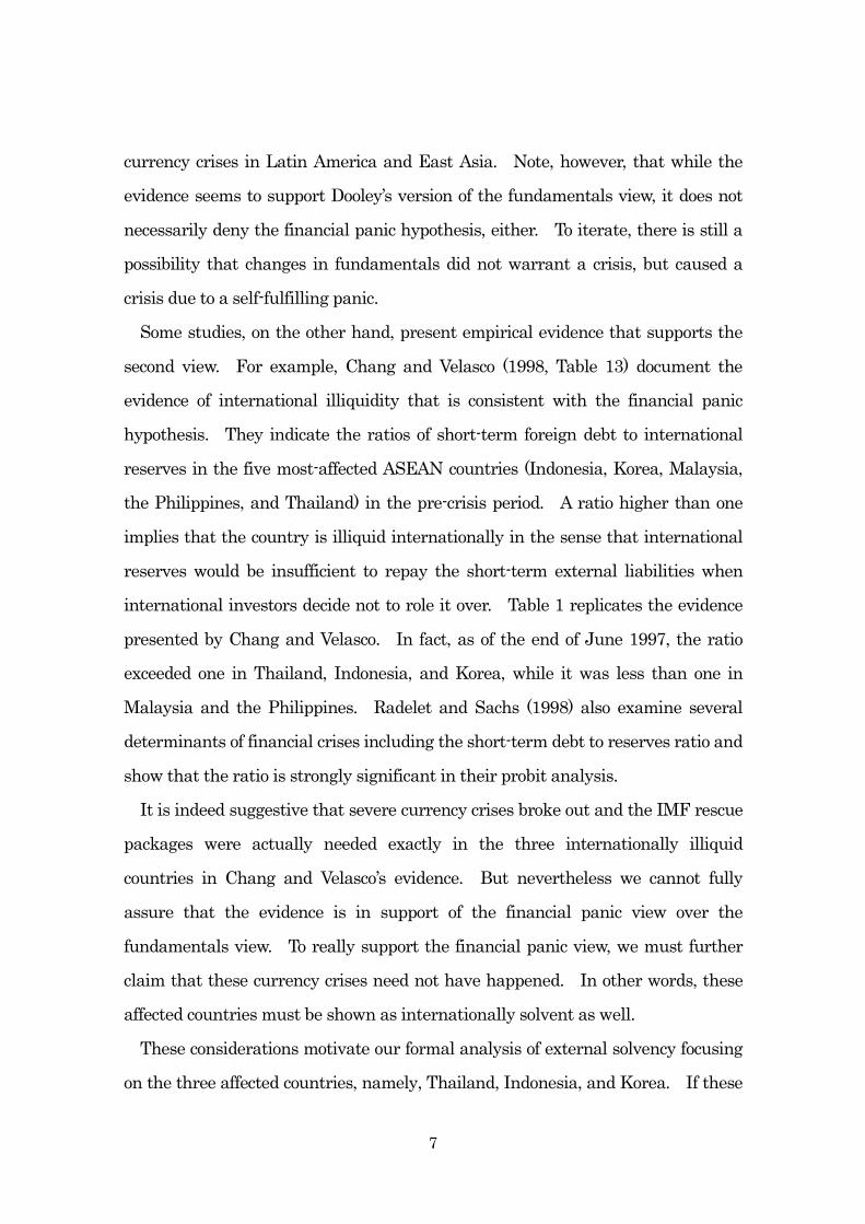
Some studies, on the other hand, present empirical evidence that supports the
second view. For example, Chang and Velasco (1998, Table 13) document the
evidence of international illiquidity that is consistent with the financial panic
hypothesis. They indicate the ratios of short-term foreign debt to international
reserves in the five most-affected ASEAN countries (Indonesia, Korea, Malaysia,
the Philippines, and Thailand) in the pre-crisis period. A ratio higher than one
implies that the country is illiquid internationally in the sense that international
reserves would be insufficient to repay the short-term external liabilities when
international investors decide not to role it over. Table 1 replicates the evidence
presented by Chang and Velasco. In fact, as of the end of June 1997, the ratio
exceeded one in Thailand, Indonesia, and Korea, while it was less than one in
Malaysia and the Philippines. Radelet and Sachs (1998) also examine several
determinants of financial crises including the short-term debt to reserves ratio and
show that the ratio is strongly significant in their probit analysis.
It is indeed suggestive that severe currency crises broke out and the IMF rescue
packages were actually needed exactly in the three internationally illiquid
countries in Chang and Velasco’s evidence. But nevertheless we cannot fully
assure that the evidence is in support of the financial panic view over the
fundamentals view. To really support the financial panic view, we must further
claim that these currency crises need not have happened. In other words, these
affected countries must be shown as internationally solvent as well.
These considerations motivate our formal analysis of external solvency focusing
on the three affected countries, namely, Thailand, Indonesia, and Korea. If these
8
countries satisfied the solvency condition, this would actually support the financial
panic view as they were already indicated as internationally illiquid. If, however,
they were shown as insolvent prior to the crisis, the fundamentals view would be a
more reasonable explanation. A formal test of external borrowing constraints
would therefore be a useful device to differentiate between these two hypotheses.
The next section explains details of our econometric framework.
3. Econometric Framework
We now describe the analytical framework based on external borrowing
constraints of an economy. We apply testing procedures developed in the
literature relating to government solvency problems (e.g. Hamilton and Flavin
1986; Hakkio and Rush 1991; Haug 1991; Trehan and Walsh 1991; and Ahmed
and Rogers 1995). Among others, Trehan and Walsh (1991) and Ahmed and
Rogers (1995) discuss a more general, stochastic environment and examine the
sustainability of external deficits as well as government deficits. This paper
adopts these two approaches.
We first explain the framework presented by Ahmed and Rogers. The current
period budget constraint of an economy is expressed as:
111 ttttttt BBYBrIC (1)
where tC is consumption, tI is investment, tr is the one-period interest rate,
tB is external debt, and tY is output, all in real terms.3
Forward substitutions of (1) yield the intertemporal budget constraint with
expectation at time t: j
kjt
kttjj
j
kjtjt
kttt B
rEMX
rEB
1 11 1 1 11lim
11
(2)
3 The term for changes in foreign currency reserves is abstracted from this derivation. The testing frameworks here will be unaffected as long as the series is stationary. And later in footnote 8, we actually confirm the stationarity of this series from unit root tests.
9
where tX and tM are exports and imports in real terms and tt MX =
ttt ICY . Then we denote jts , as marginal rate of substitution between
consumption in period t and t+j:
)('/)(', tjtj
jt CuCus (3) and assume that the Euler equation from the consumer’s optimization problem holds, i.e. 1])1[( 1,ttt srE . As demonstrated by Bohn (1995), this yields:
jtjttjjtjtj
jttt BsEMXsEB ,1
, lim)( . (4)
When the limit term on the right-hand side of equation (4) is equal to zero, the
external debt outstanding equals the expected present value of the future net
surplus. This rules out the possibility of bubble financing of the economy and is
also known as no-Ponzi game condition. The country is solvent if this condition is
satisfied.
To derive a testable implication, we take the first difference of (4), yielding:
11,11,1
, limlim)( jtjttjjtjttjjtjtj
jttt BsEBsEMXsEB . (5)
Under some certain (and plausible) conditions, Ahmed and Rogers demonstrated that the presence of a cointegrating relationship in ( tX , tM , 11 tt Br ) with the
cointegration vector (1, -1, -1) is a necessary and sufficient condition for the
present-value budget constraint to hold (i.e. the limit term in equation (4) and
therefore two limit terms in equation (5) are zero).4
The approach by Trehan and Walsh (1991) is also based on a similar stochastic
4 Key assumptions are (i) Xt and Mt are characterized as a unit root stochastic process or integrated of order one (I(1)); (ii) marginal utility of consumption (u’(Ct) ) follows a random walk; (iii) covariance between jts , and future exports and imports series (i.e. jtX or
jtM ) takes a fixed time-invariant value; and (iv) the behavior of external debt (Bt ) is considered as t
ttt uBB 1 where is a constant, 1 , and tu is a
covariance-stationary disturbance term.
10
setup. They demonstrate that if tr is a stochastic process strictly bounded below
)0( in expected value and 1tt BB is a stationary process, the external
budget constraint is satisfied. Thus stationarity of 1tt BB is a sufficient
condition for the external solvency in the Trehan-Walsh framework. 5 Note that
in this approach no assumptions are required in terms of the data generating process of the individual tX or tM series. We will employ these two
frameworks below for the case of the Asian crisis.
4. Empirical Results
4.1. Data
We use quarterly observations for the pre-crisis period of 1976:1-1997:2 for
Thailand, 1981:1-1997:2 for Indonesia, and 1976:1-1997:3 for Korea, taken from the International Financial Statistics (IFS) of the IMF.6 The series for tX , tM ,
and 11 tt Br are exports of goods and services, imports of goods and services, and
net interest payments, respectively. The change in external debt ( 1tt BB ) is
measured as the financial account in the IFS which includes net direct investment,
net portfolio investment, and other net investment, all from abroad. All the data
are deflated by consumer prices.7 The time series of these current account and
5 This is Proposition 2 of Trehan and Walsh (1991, p. 215). The basic argument here is that when 1tt BB is stationary, the expected value of external debt outstanding tB , which is the numerator of the limit term, grows at most according to a linear trend. On the other hand, the discount rate of future external debt in expected value is
)1( 11 ktjkt rE and therefore the denominator of the limit term grows exponentially.
Thus the present discounted value of future debt converges to zero and the budget constraint is satisfied. 6 The starting date for each country is given due to the availability of the IFS dataset. The sample period ends in the quarter prior to the period each country introduced the floating exchange rate regime: July 1997 for Thailand, August 1997 for Indonesia, and December 1997 for Korea. 7 The IFS codes for these data are as follows: 78aad plus 78add for exports, 78abd plus 78aed for imports, 78ahd minus 78agd for net interest payments, 78bjd for changes in external debt, and 64 for consumer prices.
11
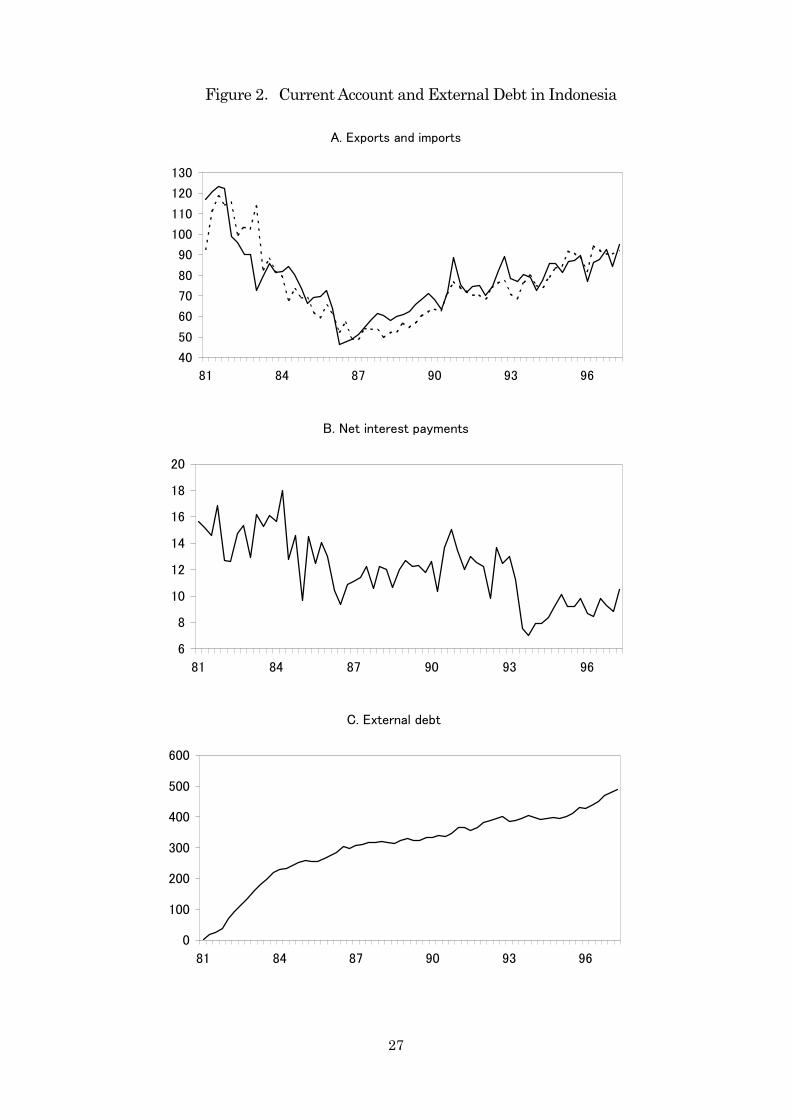
external debt data for three countries are displayed in Figures 1, 2, and 3. Graph
A shows exports (solid line) and imports (dashed line), Graph B net interest
payments, and Graph C external debt (i.e. the cumulative sum of the flow data
with the initial value being set to zero).
4.2. Solvency test I: Cointegration test among exports, imports, and net interest
payments
We first perform the solvency test by Ahmed and Roger (1995), i.e. testing
whether a cointegrating relation among exports, imports, and net interest
payments with the cointegrating vector (1, -1, -1) is supported by the pre-crisis
data in the three countries.
As a preliminary step, we check whether each of the variables are treated as I(1).
Here two unit root tests are implemented: the augmented Dickey-Fuller tests
(1979) of a unit root against no unit root (ADF), and a modified Dickey-Fuller test
based on GLS detrending series (DF-GLS), which is a powerful univariate test
proposed by Elliott, Rothenberg, and Stock (1996). Those tests include a constant
term and a linear trend for the series in levels (i.e. detrended tests) and a constant
term only for the series in first differences (i.e. demeaned tests). For Indonesia,
demeaned tests are performed for these series in levels because a time trend is not
apparent, as indicated in Graphs A and B in Figure 2. The lag length is chosen by
the Bayesian information criterion (BIC) for both of these tests (up to six lags).
Table 2 presents unit root test results (see the notes to the table for the
appropriate critical values used here). While each of the two tests does not reject
the null of a unit root for the level series, strong rejections are generally found for the first differenced series. We therefore consider that the variables tX , tM , and
11 tt Br can be all characterized as I(1).8
8 As another preliminary step, we check the stationarity of changes in foreign currency
12
Then we test for a cointegration among those three variables with the
cointegrating vector (1, -1, -1). When that cointegrating vector is imposed, the cointegration test here simply becomes a unit root test for the univariate tX - tM
- 11 tt Br series. The two unit root tests (ADF and DF-GLS) are again used in
this analysis. The tests include a constant term and the lag is chosen by the BIC.
In this analysis, we examine not only the full sample but also a subsample
spanning before rapid capital inflows appeared in each country: 1976:1-1988:4 for
Thailand, and 1981:1-1993:4 for Indonesia and Korea (see Graph C in each figure).
Furthermore, we use a subsample that ends one year before the breakout of each
crisis to see if the crises were anticipated a year before.
Table 3 shows the test results. The null is rejected by these two tests for almost
all the cases in Indonesia and Korea (see Panels B and C). The results imply that
the solvency condition was generally satisfied for the pre-crisis period in the two
countries. As for Thailand, the null is rejected for the 1988 subsample, but not for
the 1996 subsample and the full sample. This suggests that in Thailand, while
the external borrowing constraint was satisfied until the late 1980s, this was not
the case after massive capital inflows took place in the 1990s. We interpret this
evidence as indicating that the Thai crisis in July 1997 inevitably occurred because
Thailand was externally insolvent at that time. Accordingly, the fundamentals
view may be credible in Thailand. For Indonesia and Korea, the financial panic
view seems more plausible as these countries were shown as internationally
solvent but nevertheless were hit by a currency crisis.
reserves in each country (see footnote 3). We perform the same unit root tests for the series of changes in reserve assets, which is placed “below the line” on the balance of payment table (IFS code 79dbd ), and find that the null is rejected in each country. For instance, demeaned DF-GLS statistics are -2.54, -2.67, and -8.58 for Thailand, Indonesia, and Korea, respectively, and indicate strong rejections at 5 or 1% levels. We therefore interpret that the stationarity assumption is generally supported by the data.
13
4.3. Solvency test II: Unit root test for the changes in external debt
Next we conduct the solvency test of Trehan and Walsh (1991), where the stationarity of 1tt BB is examined. We once again use the two unit root tests
(ADF and DF-GLS) for 1tt BB series in each country. The tests include a
constant and the lag is selected by the BIC. The same subsample periods are
used in this exercise.
Table 4 shows the test results. In the case of Thailand (Panel A), the null of a
unit root is strongly rejected for the 1976:1-1988:4 period, which implies that the
country’s external solvency condition had been satisfied before massive capital
inflows began. With the full sample, we detect a weak rejection (10% level) by
DF-GLS, while with the 1996 subsample, no rejections are found from either of the
two tests. This suggests that around 1996, the economy was actually insolvent
and capital outflows began in the early 1997 period, which may lead to this weak
rejection result with the full sample. For Indonesia and Korea, we consistently
find rejections from DF-GLS tests with all sample periods examined. Since
DF-GLS is a more powerful procedure than ADF, we interpret this evidence as
indicating that the external solvency is generally supported in the two countries.
4.4. Analysis extending to the post-crisis period
This subsection extends our main analysis to the post-crisis period. We perform the same solvency tests as above (i.e. unit root tests for tX - tM - 11 tt Br and
1tt BB ) to see whether there is any change in the empirical results after the
crisis episodes. The extended sample period is 1976:1-2001:2 for Thailand,
1981:1-2001:1 for Indonesia, and 1976:1-2001:3 for Korea.
Table 5 summarizes the test results. It is noteworthy that with this updated,
post-crisis sample, we find strong rejections in Thailand from both tests. This
actually indicates that in a couple of years of post-crisis adjustments, the Thai
economy again becomes externally solvent. For Indonesia and Korea, the tests
14
generally detect rejections, and therefore the economies remain solvent
internationally. This suggests that a currency crisis need not happen at this
moment in any of these Asian countries.9
4.5. Further robustness check
We further perform several other exercises to check robustness of our main
findings.10 First, in solvency test I, we use different series for exports and imports
that incorporate transfer receipts and payments, respectively.11 With these
exports and imports series, the same cointegration tests are performed for the
same pre- and post-crisis sample periods. But the empirical results obtained
above are all unaffected.
Next, in solvency test II, we employ different capital flows data that exclude
direct investments from abroad.12 This may be of interest because in the Asian
crisis episodes, many observers emphasize the role of relatively short-term capital
flows such as security investments and deposits rather than long-term direct
investments. We conduct the same unit root tests for the new series, but again
the results are similar with both pre- and post-crisis samples.
Third, back to solvency test I, we perform the cointegration analysis in an unrestricted ( tX , tM , 11 tt Br ) system (i.e. without imposing the cointegrating
9 Note further that a liquidity crisis is not likely to happen, either, in any of these countries. The ratios of short-term external debt to foreign reserves (i.e. the data shown in Table 1) have been lowered considerably in the post-crisis period. As of June 2001, the ratios are 0.302, 0.649, and 0.320 for Thailand, Indonesia, and Korea, respectively, and are all well below one. They no longer indicate international illiquidity according to Chang and Velasco (1998). 10 The detailed results in this subsection are available from the author on request. 11 Both transfer series are taken from IFS (data codes are 78ajd and 78akd, respectively). Note that the transfer payments series in Indonesia is unavailable, so that only the exports series differs from the main analysis for Indonesia. Preliminary unit root tests indicate that the new exports and imports series can be characterized as I(1). 12 We substract net direct investments (IFS code 78bdd and 78bed) from the financial account data used above.
15
vector (1, -1, -1)). We implement residual-based ADF tests for cointegration.13
With this unrestricted model, some rejections indicated in Table 2 are not detected.
We interpret this as primarily being due to low power of the tests in a larger
three-variable system.14 Actually when we conduct the similar tests under a bivariate ( tX , tM + 11 tt Br ) model, some of these rejections reemerge. This
suggests that the advantage in terms of power in a more restricted, smaller system
is particularly significant for our finite-sample exercises. Accordingly, our main
results based on the univariate tests, which presumably have the largest power,
look all the more reliable.
5. Concluding Discussions
The paper has focused on two alternative views on the origins of the Asian crisis
that have been stressed in the literature: the economic fundamentals view and the
financial panic view. It has attempted to determine which of these hypotheses
best applies to the Asian crisis by testing external solvency of the relevant
countries. We have adopted procedures developed by Ahmed and Rogers (1995)
and Trehan and Walsh (1991) and examined the three most-affected countries:
Thailand, Indonesia, and Korea. The evidence indicates that while the external
solvency condition was generally satisfied in Indonesia and Korea throughout the
pre-crisis period, it was not in the case of Thailand for a pre-crisis sample
extending to the 1990s when massive capital inflows took place and external
liabilities of the economy became unsustainable. This suggests that the Thai crisis
inevitably broke out due to weak fundamentals and that the crises in Indonesia
and Korea were caused by the financial panic of international investors.
13 Detrended tests are performed for Thailand and Korea because their exports and imports series may contain a linear trend. As for Indonesia, we use demeaned tests because a time trend is not apparent in Indonesian exports and imports. 14 This is most notably in Korea. Yet robust rejections are generally found in Indonesia.
16
The econometric approach may appear overly simple as the testing procedures
involve only current account and capital account series. But arguably, it is not as
simplistic as it would seem. As seen in equations (1) and (2), key macroeconomic
variables such as private consumption and investment are at least implicitly
incorporated in the framework. Thus, those external accounts profiles reflect
current and expected spending (possibly overspending) by the private sector or the
government.
Moreover, the spending behavior in turn can be linked with the general state of
the economy and/or asset price fluctuations (such as the overheating of the
economy and a subsequent burst of asset price bubbles), and this would affect the
soundness of the financial system. These factors are usually seen as important in
the Asian crisis episodes and are incorporated in the present framework through
the spending behavior of the economy. Note further that spending decisions by
the private sector are implicitly influenced by fluctuations in relative prices and
real exchange rates that take place behind the scene.
The idea here is that all those interactions among key variables are summarized
into the simple framework based on external borrowing constraints. We therefore
view the present approach as not only simple and tractable but also reasonably
general and suitable to investigate the origins of the Asian crisis.
Before we conclude, we have two additional remarks on the interpretations of
our main findings. The first is that the evidence would also be consistent with the
“contagion” of the Asian crisis.15 The main results seem to indicate that the Thai
crisis, which broke out for the fundamentals reasons, triggered a self-fulfilling
panic in Indonesia and subsequently in Korea. Put differently, the Asian crisis
spread from the solvency crisis in Thailand to the liquidity crises in Indonesia and
15 There is also a large amount of literature on this issue. For instance, Baig and Goldfajn (1999) examined the contagion focusing on the correlation of the financial markets in the region.
17
Korea. This interpretation may provide additional insight on the mechanism of
the Asian crisis episodes.
Second, it must be emphasized that with the present approach we are still
unable to perfectly predict future crises. Even when a country is shown as
externally solvent, we cannot rule out the possibility of a liquidity crisis just as
suggested in the cases of Indonesia and Korea. Given that some crises are
actually driven by self-fulfilling financial panic, institutional arrangements to
strengthen the facility of an international lender of last resort must be seriously
discussed. While such an effort intends to reduce the likelihood of liquidity crises,
we should be fully aware that this could potentially induce moral hazard behavior
of international investors or governments and consequently could raise the
likelihood of solvency crises. Extra cautions therefore must be exercised to
develop such an international architecture to prevent future crises of both types.
18
References Ahmed, Shagill and John H. Rogers, “Government Budget Deficits and Trade Deficits: Are Present Value Constraints Satisfied in the Long-Term Data?” Journal of Monetary Economics, 36, 351-374. Baig, Tamur and Ilan Goldfajn, “Financial Market Contagion in the Asian Crisis,” IMF Staff Papers, 46 (1999), 167-195. Berg, Andrew and Catherine Pattillo, “Are Currency Crises Predictable? A Test,” IMF Staff Papers, 46 (1999), 107-138. Bohn, Henning, “The Sustainability of Budget Deficits in a Stochastic Economy,” Journal of Money, Credit and Banking, 27 (1995), 257-271. Chang, Roberto, “Origins of the Asian Crisis: Discussion,” in W. C. Hunter, G. G. Kaufman and T. H. Krueger eds., The Asian Financial Crisis: Origins, Implications and Solutions, Kluwer Academic Publishers, Boston (1998), pp. 65-71. Chang, Roberto and Andres Velasco, “The Asian Liquidity Crisis,” NBER Working Paper No. 6796, November 1998. Chang, Roberto and Andres Velasco, “Financial Fragility and the Exchange Rate Regime,” Journal of Economic Theory, 92 (2000), 1-34. Chang, Roberto and Andres Velasco, “A Model of Financial Crises in Emerging Markets,” Quarterly Journal of Economics, May 2001, 489-517. Chinn, Menzie D., Michael P. Dooley, and Sona Shrestha, “Latin America and East Asia in the Context of an Insurance Model of Currency Crises,” Journal of International Money and Finance, 18 (1999), 659-681. Dickey, D. A. and W. A. Fuller, “Distribution of the Estimators for Autoregressive Time Series with a Unit Root,” Journal of American Statistical Association, 74 (1979), 427-431. Dooley, Michael P., “A Model of Crises in Emerging Markets,” Economic Journal, 110 (2000), 256-272. Elliott, Graham, Thomas J. Rothenberg, and James H. Stock, “Efficient Tests for an
19
Autoregressive Unit Root,” Econometrica, 64 (1996), 813-836. Fuller, W. A., Introduction to Statistical Time Series, New York: John Wiley and Sons, 1976. Furman, Jason and Joseph E. Stiglitz, “Economic Crises: Evidence and Insights from East Asia,” Brookings Papers on Economic Activity, 2 (1998), 1-135. Glick, Reuven, “Thoughts on the Origins of the Asian Crisis: Impulses and Propagation Mechanisms,” in W. C. Hunter, G. G. Kaufman and T. H. Krueger eds., The Asian Financial Crisis: Origins, Implications and Solutions, Kluwer Academic Publishers, Boston (1998), pp. 33-63. Goldfajn, Ilan and Rodrigo O. Valdes, “Are Currency Crises Predictable?” European Economic Review, 42 (1998), 873-885. Hakkio, Craig S. and Mark Rush, “Is the Budget Deficit ‘Too Large’?” Economic Inquiry, 29 (1991), 429-445. Hamilton, J. D. and M. Flavin, “On the Limitation of Government Borrowing: A Framework for Empirical Testing,” American Economic Review, 76 (1986), 808-819. Haug, Alfred A., “Cointegration and Government Borrowing Constraints: Evidence for the United States,” Journal of Business and Economic Statistics, 9 (1991), 97-101. Ito, Takatoshi, “Capital Flows in Asia,” NBER Working Paper No. 7134 (1999). Kaminsky, Graciela, Saul Lizondo, and Carmen M. Reinhart, “Leading Indicators of Currency Crises,” IMF Staff Papers, 45 (1998), 1-48. Krugman, Paul, “A Model of Balance-of-Payments Crises,” Journal of Money, Credit, and Banking, 11 (1979), 311-325. Miyao, Ryuzo, “Another Look at Origins of the Asian Crisis: Tests of External Borrowing Constraints,” ESRI Discussion Paper No. 11, Economic and Social Research Institute, Cabinet Office of Japan, February 2002. Obstfeld, Maurice, “Rational and Self-Fulfilling Balance of Payments Crises,” American Economic Review, 76 (1986), 72-81.
20
Radelet, Steven and Jefrrey D. Sachs, “The East Asian Financial Crisis: Diagnosis, Remedies, Prospects,” Brookings Papers on Economic Activity, 1 (1998), 1-90. Sawada, Yasuyuki, “Are the Heavily Indebted Countries Solvent? Tests of Interemporal Budget Constraints,” Journal of Development Economics, 45 (1994), 325-337. Trehan, Bharat and Carl E. Walsh, “Testing Intertemporal Budget Constraints: Theory and Applications to U.S. Federal Budget and Current Account Deficits,” Journal of Money, Credit and Banking, 23 (1991), 206-223.
21
Table 1. Short-Term External Debt to Reserves Ratio ———————————————————————————————————————— Period Thailand Indonesia Korea Malaysia Philippines
———————————————————————————————————————— Notes: This table replicates the evidence on international illiquidity shown by Chang and Velasco (1998, Table 13). It reports the ratio of short-term external debt to international reserves at the end of the second quarter (June) of each year. Short-term debt is the series “liabilities to banks, due within a year” taken from the Bank for International Settlements (BIS) statistics on external debt, and international reserves series is retrieved from IMF International Financial Statistics (line 1d.d).
22
Table 2. Unit Root Test Results ― For exports, imports, and net interest payments ―
Δrt-1Bt-1 -7.43(2)** -6.80(2)** ————————————————————————————————————————— Notes: This table reports statistics testing for a unit root for exports (Xt ), imports (Mt ), and net interest payments (rt-1Bt-1), all deflated by CPI, in the three Asian countries. ADF is the augmented Dickey-Fuller test (1979) of a unit root against no unit root and DF-GLS is a Dickey-Fuller test based on GLS-detrended series, proposed by Elliott, Rothenberg, and Stock (1996). The tests include a constant and a linear trend for the series in levels (i.e. detrended tests) and a constant term only for the series in first differences (i.e. demeaned tests). As for Indonesia, demeaned tests are performed for the series in levels since a linear trend is not apparent in Figure 2. The sample period is 1976:1-1997:2 for Thailand, 1981:1-1997:2 for Indonesia, and 1976:1-1997:3 for Korea. The lag lengths shown in the parentheses are chosen based on the BIC (up to six lags). Critical values, tabulated by Fuller (1976) and Elliott, Rothenberg, and Stock (1996), are:
B. Indonesia 81:1-93:4 -2.76(4)† -2.05(4)* 81:1-96:2 -2.95(4)* -1.88(4)† 81:1-97:2 -3.12(4)* -1.99(4)*
C. Korea 76:1-93:4 -2.63(0)† -2.41(0)* 76:1-96:3 -2.53(0) -2.43(0)* 76:1-97:3 -3.05(0)* -2.92(0)** ———————————————————————————————————————— Notes: This table reports statistics testing for cointegration among exports, imports, and net interest payments with cointegrating vector (1, -1, -1), i.e. testing for a unit root for Xt
-Mt-rt-1Bt-1. ADF is the augmented Dickey-Fuller test (1979) of a unit root against no unit root and DF-GLS is a Dickey-Fuller test based on GLS-detrended series, proposed by Elliott, Rothenberg, and Stock (1996). Those tests include a constant term (i.e. demeaned tests). The lag lengths shown in the parentheses are chosen based on BIC (up to six lags). Critical values, tabulated by Fuller (1976) and Elliott, Rothenberg, and Stock (1996), are: 10%(†) 5%(*) 1%(**) ADF -2.58 -2.89 -3.51 DF-GLS -1.61 -1.95 -2.60
24
Table 4. Solvency Test II
― Unit root tests for changes in external debt ―
———————————————————————————————————————— Period ADF DF-GLS
———————————————————————————————————————— A. Thailand
B. Indonesia 81:1-93:4 -2.23(4) -2.06(4)* 81:1-96:2 -2.46(4) -2.03(4)* 81:1-97:2 -2.29(4) -1.78(4)†
C. Korea 76:1-93:4 -2.49(1) -2.28(1)* 76:1-96:3 -2.38(1) -2.35(1)* 76:1-97:3 -2.49(1) -2.45(1)* ———————————————————————————————————————— Notes: This table reports statistics testing for a unit root for changes in external debt (Bt
-Bt-1). ADF is the augmented Dickey-Fuller test (1979) of a unit root against no unit root and DF-GLS is a Dickey-Fuller test based on GLS-detrended series, proposed by Elliott, Rothenberg, and Stock (1996). The tests include a constant term (i.e. demeaned tests). The lag lengths shown in the parentheses are chosen based on the BIC (up to six lags). Critical values, tabulated by Fuller (1976) and Elliott, Rothenberg, and Stock (1996), are: 10%(†) 5%(*) 1%(**) ADF -2.58 -2.89 -3.51 DF-GLS -1.61 -1.95 -2.60
25
Table 5. Additional Results
― For samples extended to the post-crisis period ―
B. Indonesia Xt-Mt-rt-1Bt-1 -2.60(4)† -2.13(4)* Bt-Bt-1 -4.05(0)** -3.79(0)**
C. Korea Xt-Mt-rt-1Bt-1 -2.80(0)† -2.54(0)* Bt-Bt-1 -5.88(0)** -5.67(0)** ——————————————————————————————————————— Notes: This table reports statistics testing for a unit root for Xt-Mt-rt-1Bt-1 and Bt-Bt-1 (i.e. the solvency tests I and II) for updated samples extending to the post-crisis period. The sample period is 1976:1-2001:2 for Thailand, 1981:1-2001:1 for Indonesia, and 1976:1-2001:3 for Korea. ADF is the augmented Dickey-Fuller test (1979) of a unit root against no unit root and DF-GLS is a Dickey-Fuller test based on GLS-detrended series, proposed by Elliott, Rothenberg, and Stock (1996). The tests include a constant term (i.e. demeaned tests). The lag lengths shown in the parentheses are chosen based on the BIC (up to six lags). Critical values, tabulated by Fuller (1976) and Elliott, Rothenberg, and Stock (1996), are: 10%(†) 5%(*) 1%(**) ADF -2.58 -2.89 -3.51 DF-GLS -1.61 -1.95 -2.60
26
Figure 1. Current Account and External Debt in Thailand
A. Exports and imports
0
20
40
60
80
100
120
140
160
180
200
76 79 82 85 88 91 94 97
B. Net interest payments
0
1
2
3
4
5
6
7
8
9
10
76 79 82 85 88 91 94 97
C. External debt
0
100
200
300
400
500
600
700
800
900
1000
76 79 82 85 88 91 94 97
27
Figure 2.Current Account and External Debt in Indonesia
A. Exports and imports
40
50
60
70
80
90
100
110
120
130
81 84 87 90 93 96
B. Net interest payments
6
8
10
12
14
16
18
20
81 84 87 90 93 96
C. External debt
0
100
200
300
400
500
600
81 84 87 90 93 96
28
Figure 3.Current Account and External Debt in Korea