21
AN EMPIRICAL TEST OF THE EFFECT
OF BASIS RISK ON CASH MARKET POSITIONS
Janet S. Netz
Purdue University
Abstract: Traditional theory holds that hedgers use futures markets to reduce the amount
of price risk they bear. In doing so, they trade price risk for basis risk, that is, unexpected
movements in the di�erence between the spot and futures prices. Theoretical work has
shown that the presence of basis risk reduces output (of which storage is a special case)
and the relative use of futures as a hedging instrument. This paper attempts to empirically
measure the e�ect of basis risk on the cash market position. This study empirically tests
the implication of reduced storage in the face of basis risk using data on the storage of corn.
Results show that basis risk statistically and economically signi�cantly reduces the level of
storage. The implications of basis risk on cash market positions extend beyond commodity
storage to any hedging situation, including the use of currency futures to insure against
exchange rate risk.
Acknowledgements: I would like to thank Severin Borenstein, Alan Deardor�, Jon Haveman, Jim
Levinsohn, Je� MacKie-Mason, Craig Pirrong, and seminar participants at the University of California
at Davis for helpful comments. The Center for the Study of Futures Markets at Columbia University
generously provided futures price data.
Address: 1310 Krannert, W. Lafayette, IN 47907-1310 E-mail: [email protected]

AN EMPIRICAL TEST OF THE EFFECT
OF BASIS RISK ON CASH MARKET POSITIONS
Janet S. Netz
A large literature, theoretical and empirical, explores the e�ect of basis risk on
the e�ectiveness of futures markets as a risk management tool and on the hedge ratio. It
is widely accepted and empirically proven that, in the face of basis risk, the hedge ratio
should be less than one.1 Because basis risk a�ects the hedging e�ectiveness of futures
markets, work has also been done on empirically determining what variables a�ect the basis
(the di�erence between the cash and futures prices) and basis risk (unexpected changes in
the basis over time).2
Despite the abundance of work on the e�ect of basis risk on futures markets
positions, economists have largely ignored the e�ect of basis risk on cash market positions.
Paroush and Wolf (1989, 1992) and Anderson and Danthine (1981) have theoretically
shown that basis risk a�ects the cash market position, but the theoretical results have not
been empirically tested. This paper �lls this void by testing the e�ect of basis risk on the
cash market position.
Intuitively, why should basis risk matter? The importance of the basis and basis
risk arises because very few contracts (less than 3%) are o�set through delivery. To illus-
trate, consider a simple case of a storer who takes a position in the cash market and the
1 Estimates range from a low of .3 to close to 1. See Peck (1975) for eggs; Ederington (1979) for wheat,corn, GNMAs, and T-bills; Figlewski (1984) for S&P 500 index futures; Castelino (1992) for wheat,corn, T-bills and Eurodollars; and Moser and Helms (1990) for British pounds, Canadian dollars,Deutschemarks, and Swiss Francs.
2 Vollink and Raikes (1977) analyze the live cattle basis; Tilley and Campbell (1988) the wheat basis;Martin, Groenewegen, and Pidgeon (1980) the corn basis; Ward and Dasse (1977) the frozen concen-trated orange juice basis; Garcia, Leuthold, and Sarhan (1984) livestock basis; and Figlewski (1984)the S&P 500 Index basis. The latter two also analyze the determinants of basis risk.
1

futures market in period 1 and reverses the position in period 2. She buys the cash good
at c1 and sells at c2, and sells the futures contract at f1 and buys at f2. Her pro�ts are
(c2� c1)+(f1 �f2), or, in terms of the basis, bi = ci�fi, b2� b1. Thus, the change in the
basis over the life of the hedge determines the agent's pro�ts. The riskiness or variance of
the storer's pro�ts will be a function of the variance of the basis.3 Since basis risk a�ects
the risk of pro�ts from the hedged position, it seems likely that it a�ects the cash position.
In particular, basis risk should reduce the cash position of risk-averse agents.
More precisely, unexpected changes in the basis a�ect the riskiness of the hedge.
The basis is expected to change over the life of the hedge. In particular, for storable
commodities, the basis will change by the change in the storage costs over the period.
That is, the theory of storage (Working (1949)) suggests that the basis should be equal to
no more than the cost of storage between today and the expiration date of the contract.
If the basis were higher than the costs of storage, an arbitrage opportunity would exist.
Thus, if the hedge were opened two months before the contract expiration date and closed
one month before expiration, the basis should narrow by one month's storage cost. Because
this change in basis is expected, it should not be considered risk.
Section II begins with a standard portofolio model of storage and hedging to
illustrate that an increase in basis risk reduces the cash market position. In contrast to
initial portfolio approaches to hedging (Stein (1961)), both the cash and futures positions
are endogenous.4 Then other theoretical papers are discussed to show that the result is
fairly general and not dependent on the functional form used or other assumptions. The
result is that as either basis risk or price risk increases, the agent will reduce the level of
inventories. Section III develops an empirical test of the hypothesis that basis risk a�ects
the cash market position and discusses the empirical methodology. The model is applied
to the storage of corn. This application is chosen since detailed data on corn are available
3 This simple example assumes a complete hedge (a hedge ratio of 100%). A more realistic model isdeveloped below.
4 Obviously if the cash position were exogenous, basis risk would not a�ect it.
2
from the U.S.D.A. Data are used to estimate storage at the nine major corn markets
in the United States using weekly data from 1984 to 1989.5;6 Section IV describes the
data. Section V presents the results, which demonstrate that basis risk has a signi�cant
negative impact on the level of storage. Section VI summarizes the paper and discusses
the implications and future research.
II. The Model
The impact of basis risk on the cash and futures positions can be illustrated using
a standard mean-variance model of storage (e.g., Turnovsky (1983)). After illustrating the
e�ect of basis risk on the level of inventories, I discuss other models that incorporate basis
risk to show that basis risk negatively a�ects the cash position under other assumptions
and approaches.
Assume a perfectly competitive, risk-averse agent faces uncertainty and uses fu-
tures contracts to manage risk. Risk arises in this application because the output price is
unknown. The storer is motivated by intertemporal arbitrage.7 Storage costs are assumed
to be linear, and the production function is one-to-one, so that one unit of input (grain
today) gives one unit of output (grain tomorrow).8 The futures market is assumed to be
perfectly competitive and populated by a large number of risk-neutral speculators. Thus,
hedgers take the futures price as given. For simplicity, a mean-variance approach is taken.
Variables are de�ned as: pt is the spot price in period t; a tilde over any variable
indicates that it is a random variable; st denotes storage from period t to period t+1; r is
the interest rate; e and F are positive constants, where e is the per unit cost of storage and
5 Basis risk varies over time and across location because the futures price and local spot prices will besubject to di�erent shocks over time.
6 The working paper version of this manuscript also used data on storage of soybeans. The applicationwas awed because it only considered soybean contracts. A soybean storer can also use soybean oiland meal contracts to hedge. Basis risk arising from the soybean contract could lead to a re-allocationto meal and oil contracts rather than a�ecting the cash position. A more sophisticated empirical testwhich included data on the relationship between the cash price and the three futures prices wouldbe required. See Anderson and Danthine (1981) for a model of hedging with multiple contracts.
7 This assumption is relaxed below.8 Spoilage is ignored in the model.
3

F is the �xed cost of storage; zt is the number of contracts sold (purchased if zt < 0); fi;j
is the price in period i of a futures contract that expires in j; A is the coe�cient of absolute
risk aversion; txt+1 is the time t expectation of variable x in the following period; �2i (�i)
is the variance (standard deviation) of variable i; and �ij is the covariance of variables i
and j.
The storer solves the following maximization problem:
maxst;zt
�t pt+1
1 + r� pt
�st � (est + F )
+
�ft;t+1 � t ft+1;t+1
1 + r
�zt
�1
2A
s2t(1 + r)2
�2p �1
2A
z2t(1 + r)2
�2f +Astzt
(1 + r)2�pf
s:t: st � 0:
The �rst two terms represent the expected pro�ts from storage, the third term represents
the expected pro�ts from selling futures,9 and the last three terms represent the e�ect on
utility arising from uncertainty. An increase in the variance of either the spot or futures
price reduces utility because the increased variance indicates that operations in the spot
or futures market, respectively, are riskier. The covariance term raises utility.10 This term
increases utility because it represents hedging; losses in one market are o�set, to some
extent, by gains in the other market.
This model yields the same implications of basis risk on the futures position as
previous studies. Optimization yields the standard hedging position
zt =(ft � t ft+1)
A(1 + r)�1�2f
+�pf
�2f
st: (1)
The two terms are the speculative and hedging components, respectively. Assuming that
a large number of risk-neutral speculators operate in the futures market, equilibrium in
9 Transactions costs in the futures market are ignored.10 As shown below, the position in the futures market (short or long) depends on the sign of the
covariance between the spot and futures prices (positive or negative); thus the �nal term is alwayspositive.
4
the futures market requires that speculative pro�ts be zero, in which case ft = tft+1.11 In
this case, the speculative (�rst) term disappears, and the optimal futures position is some
fraction of the inventory level for an interior solution and zero for a corner solution.
The hedge ratio is given by �pf =�2f, or alternatively as (�p=�f )�pf , where � is the
correlation coe�cient between the spot and futures price over the life of the hedge. So long
as the futures and cash prices are positively correlated, as they will be when the stocks
and the futures contract are based on the same fundamental commodity (e.g., corn futures
and corn inventories), then the agent will take opposite positions in the two markets. That
is, a storer will o�set inventories of corn by selling corn futures. As price risk rises (as
measured by the standard deviation of the spot price), the hedge ratio increases, that is,
the agent hedges more of the inventory using futures markets. As basis risk rises (� or �pf
falls), the agent reduces the futures position for a given level of inventories. Intuitively,
the futures market is not as good an instrument for managing price risk when basis risk is
present; therefore the agent relies on futures less, insuring a fraction of stocks with futures
and self-insuring the remainder.
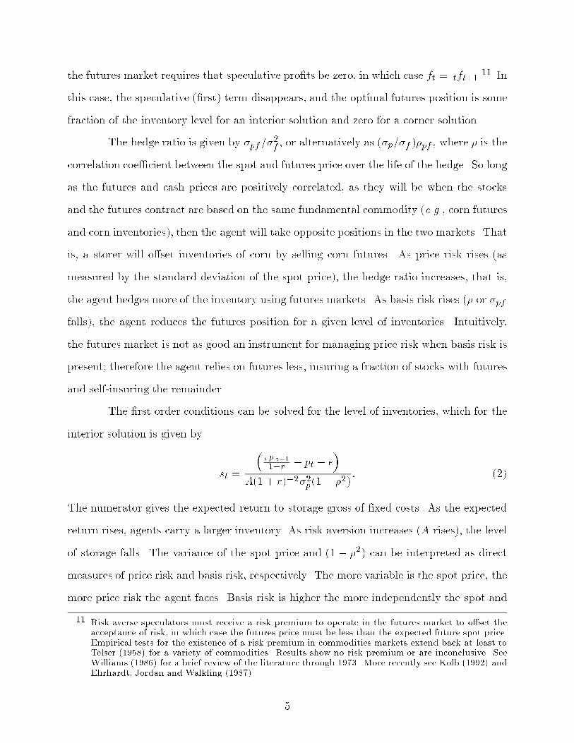
The �rst order conditions can be solved for the level of inventories, which for the
interior solution is given by
st =
�t p t+1
1+r � pt � e�
A(1 + r)�2�2p(1� �2): (2)
The numerator gives the expected return to storage gross of �xed costs. As the expected
return rises, agents carry a larger inventory. As risk aversion increases (A rises), the level
of storage falls. The variance of the spot price and (1 � �2) can be interpreted as direct
measures of price risk and basis risk, respectively. The more variable is the spot price, the
more price risk the agent faces. Basis risk is higher the more independently the spot and
11 Risk-averse speculators must receive a risk premium to operate in the futures market to o�set theacceptance of risk, in which case the futures price must be less than the expected future spot price.Empirical tests for the existence of a risk premium in commodities markets extend back at least toTelser (1958) for a variety of commodities. Results show no risk premium or are inconclusive. SeeWilliams (1986) for a brief review of the literature through 1973. More recently see Kolb (1992) andEhrhardt, Jordan and Walkling (1987).
5

futures prices move over the life of the hedge ((1��2) is high). For each of these measures
of risk, as risk increases, storage decreases.
The corner solution states that storage is zero when the return to storage is non-
positive. However, storage is often observed to be positive even when the return is negative.
To explain this observed paradox, Kaldor (1939) and Brennan (1958) introduced the con-
cept of convenience yield. The intuitively appealing idea is that agents �nd it convenient to
hold inventory. This convenience may arise, for example, because it allows agents to meet
unexpected demand. Convenience yield is assumed to be a non-linear function of storage,
with a negative �rst and positive second derivative. With convenience yield, positive stor-
age may occur with a negative return because of the convenience it gives the agent. Taking
the maximization problem for a risk-averse storer and adding convenience yield leads to
the following implicit interior solution for the level of storage
stA�2p(1 � �2)
(1 + r)2� c0(st) =
t p t+1
1 + r� pt � e;
where c(st) is convenience yield as a function of the level of inventories. Total di�erentiation
shows that storage decreases as price risk or basis risk rises (and increases as the return
to storage rises).
Thus, risk-averse agents who store to make pro�ts from intertemporal arbitrage
will hold less inventory in the face of increased basis or price risk, regardless of whether
they also hold inventories for convenience yield purposes.
Anderson and Danthine (1981) present a model of hedging with multiple contracts
(of which this model is a special case with one futures contract). Their model is also more
general in that they do not make the assumption that ft = tft+1. In that case, it is
possible for basis risk to increase the cash market position. However, this occurs only
when speculative pro�ts from buying futures (ft < tft+1) when the hedge is opened are
so large that speculative buying o�sets hedge selling, so that the agent is long both cash
and futures. As pointed out by Peck (1975), this seems unlikely to occur. In any event,
their work shows that the cash position will not be independent of basis risk.
6
Paroush and Wolf (1989) maximize the expected utility as a function of pro�ts of
a �rm that operates in a cash market and has access to a futures market in a two-period
model. In the �rst period the �rm commits to its position in the cash and futures markets;
in the second the �rm sells the product in the cash market and closes its futures position.
Thus, pro�ts are given by �t = pt+1st + (ft;t+1 � ft+1;t+1)zt � c(st) (changing Paroush
and Wolf's notation to match that above). To apply their model to the case of storage,
c(st) should be de�ned as ptst. Paroush and Wolf assume that the cash price is equal
to a mean value plus a normally distributed random shock. The futures price is a linear
function of the spot price plus another, independently normally distributed random error.
The random errors can be interpreted as price risk and basis risk, respectively. Paroush
and Wolf show that production (or storage) in the presence of basis risk is less than in the
absence of basis risk, and that production (or storage) declines as basis risk rises.12
Thus, under a variety of assumptions and approaches, basis risk reduces the cash
market position as well as reducing the hedge ratio. This paper proceeds to empirically
test the result.
III. Empirical Methodology
The model indicates that storage, from the point of view of an individual risk-
averse agent, is a function of the return to storage, basis risk, and price risk. At the
market level, storage will also depend on the amount available to be stored. To capture
these e�ects, the following equation is estimated
st = �+ �1 rett + 1 brskt + 2 prskt + �2 prodnt + �t; (1e)
where
s = the level of storage, in thousand bushels;
12 In a separate paper, Paroush and Wolf (1992) theoretically examine the impact of basis risk on thedemand for inputs (for example, our millers). They �nd that as basis risk increases, demand forthe risky input declines, another example where basis risk a�ects a cash market position.
7
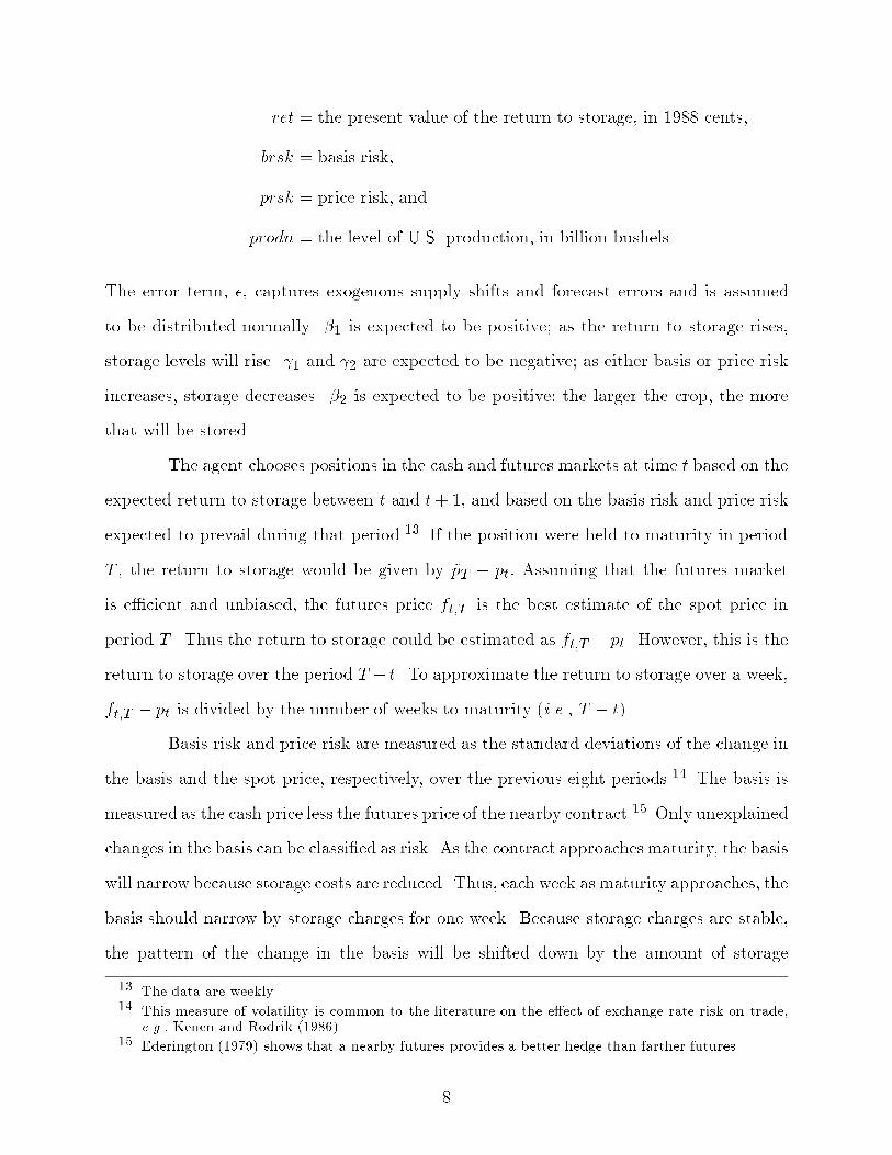
ret = the present value of the return to storage, in 1988 cents,
brsk = basis risk,
prsk = price risk, and
prodn = the level of U.S. production, in billion bushels.
The error term, �, captures exogenous supply shifts and forecast errors and is assumed
to be distributed normally. �1 is expected to be positive; as the return to storage rises,
storage levels will rise. 1 and 2 are expected to be negative; as either basis or price risk
increases, storage decreases. �2 is expected to be positive; the larger the crop, the more
that will be stored.
The agent chooses positions in the cash and futures markets at time t based on the
expected return to storage between t and t+ 1, and based on the basis risk and price risk
expected to prevail during that period.13 If the position were held to maturity in period
T , the return to storage would be given by ~pT � pt: Assuming that the futures market
is e�cient and unbiased, the futures price ft;T is the best estimate of the spot price in
period T . Thus the return to storage could be estimated as ft;T � pt. However, this is the
return to storage over the period T � t. To approximate the return to storage over a week,
ft;T � pt is divided by the number of weeks to maturity (i.e., T � t).
Basis risk and price risk are measured as the standard deviations of the change in
the basis and the spot price, respectively, over the previous eight periods.14 The basis is
measured as the cash price less the futures price of the nearby contract.15 Only unexplained
changes in the basis can be classi�ed as risk. As the contract approaches maturity, the basis
will narrow because storage costs are reduced. Thus, each week as maturity approaches, the
basis should narrow by storage charges for one week. Because storage charges are stable,
the pattern of the change in the basis will be shifted down by the amount of storage
13 The data are weekly.14 This measure of volatility is common to the literature on the e�ect of exchange rate risk on trade,
e.g., Kenen and Rodrik (1986).15 Ederington (1979) shows that a nearby futures provides a better hedge than farther futures.
8

charges. Thus the standard deviation of the change in the basis will be unchanged. Tilley
and Campbell show that the contract a�ects the level of the basis. Since the standard
deviation of changes in the basis are used as the measure of risk, the di�erent basis level
for each contract will be di�erenced out, so that this e�ect is not a source of bias in
the measure of basis risk. Furthermore, Garcia, Leuthold, and Sarhan (1984) �nd little
evidence that basis risk changes as maturity approaches.
Applying the Cochrane-Orcutt procedure to equation (1e) provides estimates of
the degree of serial correlation at about .97 or higher at each location, which suggests the
presence of a unit root (non-stationarity).16 Univariate tests for non-stationarity, involving
regressing the variable on its lag, its lag and a constant, or its lag, a constant and a time
trend, and a multivariate test for non-stationarity give similar results.17 Storage is non-
stationary, except for Peoria; however, even the result at Peoria is borderline. To eliminate
non-stationarity, equation (1e) is estimated in di�erences.
The return to storage (ret) is clearly correlated with the error term since the
return to storage and the level of storage are determined simultaneously. A high return
to storage leads to higher levels of storage, but higher levels of storage lead to a lower
return to storage. Thus standard estimation will result in a coe�cient estimate that
is biased downward. To the extent that the return to storage is correlated with basis
risk and price risk, the coe�cients on these variables will also be biased. To control for
simultaneity, I use intrumental variables in a two-stage least squares framework. The
identifying instruments used are the yield of the surrounding farm area, the amount of
corn inspected for export, the amount of corn shipped by waterways, state rainfall and
temperature, and monthly dummies. Rainfall, temperature and monthly dummies are
16 See Plosser and Schwert (1978) for an excellent non-technical discussion of the implications of a unitroot, as well as how di�erent estimating techniques in the presence of a unit root can lead to di�erentinferences.
17 The multivariate test is derived by quasi-di�erencing equation (1e), adding (st�st�1) to both sides,and adding and subtracting the one-period lag of each independent variable to the RHS. To test forstationarity, the transformed equation is estimated using OLS. Under the null hypothesis of a unitroot, the coe�cients on the lagged dependent variable and the lagged independent variables shouldall be zero. The test statistic on the lagged dependent variable will be distributed as �̂� in Fuller(1976), and the test statistic on the other coe�cients will follow the standard t-distribution.
9
clearly exogenous. The yield will help explain the return to storage in the following way:
the higher the yield, the less need to spread the crop over the crop-year, and the lower the
return to storage. Precipitation, temperature, and monthly dummies are other proxies for
such supply e�ects. The amount of corn shipped by waterways and the amount inspected
for export will a�ect the return to storage through changes in supply and demand.
The application of the empirical test involves storage at nine locations. The data
are pooled over the nine locations and the six years. Chow tests for structural change
accept the hypothesis that coe�cients are equal across locations and years.
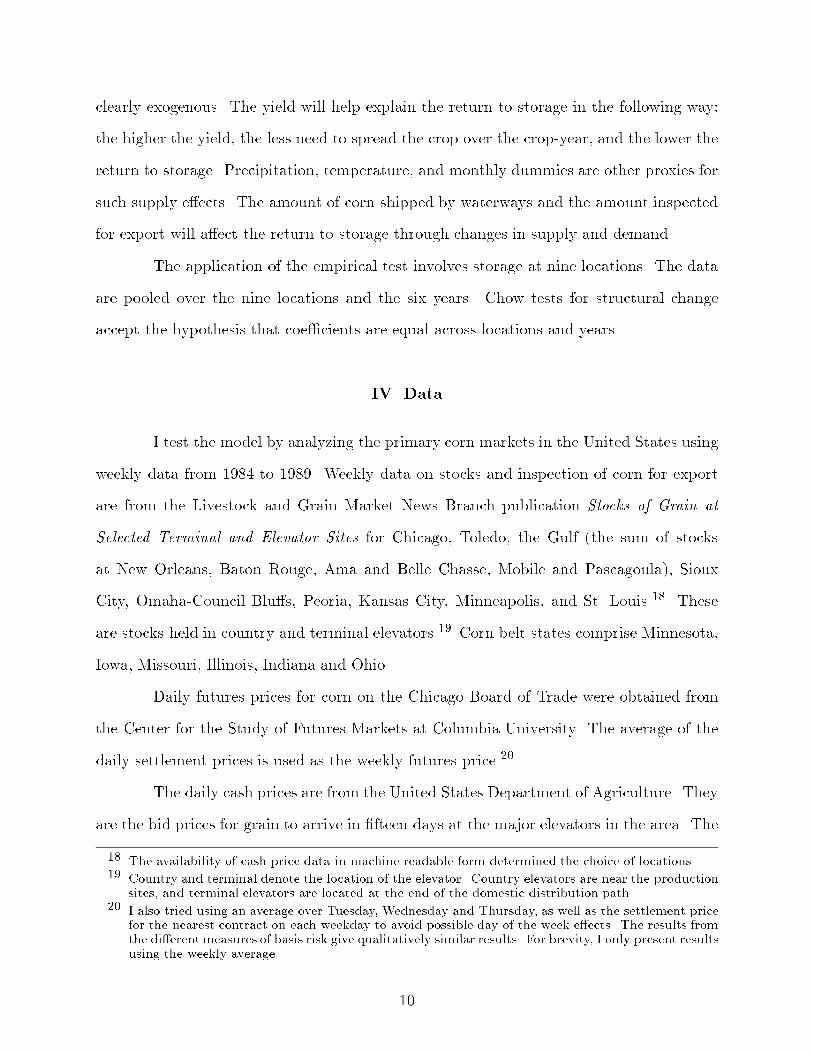
IV. Data
I test the model by analyzing the primary corn markets in the United States using
weekly data from 1984 to 1989. Weekly data on stocks and inspection of corn for export
are from the Livestock and Grain Market News Branch publication Stocks of Grain at
Selected Terminal and Elevator Sites for Chicago, Toledo, the Gulf (the sum of stocks
at New Orleans, Baton Rouge, Ama and Belle Chasse, Mobile and Pascagoula), Sioux
City, Omaha-Council Blu�s, Peoria, Kansas City, Minneapolis, and St. Louis.18 These
are stocks held in country and terminal elevators.19 Corn belt states comprise Minnesota,
Iowa, Missouri, Illinois, Indiana and Ohio.
Daily futures prices for corn on the Chicago Board of Trade were obtained from
the Center for the Study of Futures Markets at Columbia University. The average of the
daily settlement prices is used as the weekly futures price.20
The daily cash prices are from the United States Department of Agriculture. They
are the bid prices for grain to arrive in �fteen days at the major elevators in the area. The
18 The availability of cash price data in machine readable form determined the choice of locations.19 Country and terminal denote the location of the elevator. Country elevators are near the production
sites, and terminal elevators are located at the end of the domestic distribution path.20 I also tried using an average over Tuesday, Wednesday and Thursday, as well as the settlement price
for the nearest contract on each weekday to avoid possible day of the week e�ects. The results fromthe di�erent measures of basis risk give qualitatively similar results. For brevity, I only present resultsusing the weekly average.
10
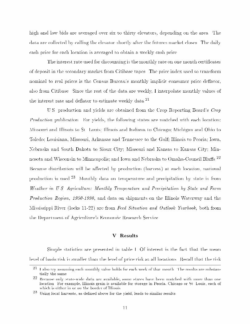
high and low bids are averaged over six to thirty elevators, depending on the area. The
data are collected by calling the elevator shortly after the futures market closes. The daily
cash price for each location is averaged to obtain a weekly cash price.
The interest rate used for discounting is the monthly rate on one-month certi�cates
of deposit in the secondary market from Citibase tapes. The price index used to transform
nominal to real prices is the Census Bureau's monthly implicit consumer price de ator,
also from Citibase. Since the rest of the data are weekly, I interpolate monthly values of
the interest rate and de ator to estimate weekly data.21
U.S. production and yields are obtained from the Crop Reporting Board's Crop
Production publication. For yields, the following states are matched with each location:
Missouri and Illinois to St. Louis; Illinois and Indiana to Chicago; Michigan and Ohio to
Toledo; Louisiana, Missouri, Arkansas and Tennessee to the Gulf; Illinois to Peoria; Iowa,
Nebraska and South Dakota to Sioux City; Missouri and Kansas to Kansas City; Min-
nesota and Wisconsin to Minneapolis; and Iowa and Nebraska to Omaha-Council Blu�s.22
Because distribution will be a�ected by production (harvest) at each location, national
production is used.23 Monthly data on temperature and precipitation by state is from
Weather in U.S. Agriculture: Monthly Temperature and Precipitation by State and Farm
Production Region, 1950-1990, and data on shipments on the Illinois Waterway and the
Mississippi River (locks 11-22) are from Feed Situation and Outlook Yearbook, both from
the Department of Agriculture's Economic Research Service.
V. Results
Simple statistics are presented in table I. Of interest is the fact that the mean
level of basis risk is smaller than the level of price risk at all locations. Recall that the risk
21 I also try assuming each monthly value holds for each week of that month. The results are substan-tially the same.
22 Because only state-wide data are available, some states have been matched with more than onelocation. For example, Illinois grain is available for storage in Peoria, Chicago or St. Louis, each ofwhich is either in or on the border of Illinois.
23 Using local harvests, as de�ned above for the yield, leads to similar results.
11

Table I
Descriptive Statistics
(Standard Deviations in Parentheses)
Location Cash Price1 Stocks2 Price Risk Basis Risk
St. Louis 2.41 (0.37) 1,777 (1,973) 7.39 (5.61) 5.41 (3.66)
Chicago 2.32 (0.37) 12,414 (9,436) 7.48 (5.20) 5.30 (3.64)
Toledo 2.33 (0.39) 18,372 (9,701) 6.98 (5.03) 4.91 (3.21)
Gulf 2.59 (0.37) 6,292 (2,684) 7.48 (5.36) 5.19 (3.26)
Peoria 2.26 (0.38) 2,020 (794) 6.96 (5.27) 5.07 (3.39)
Sioux City 2.14 (0.40) 4,765 (2,171) 6.40 (4.75) 5.01 (2.81)
Kansas City 2.33 (0.38) 5,805 (1,964) 6.95 (4.58) 5.04 (2.41)
Minneapolis 2.27 (0.38) 12,040 (5,288) 8.65 (8.69) 7.20 (8.28)
Omaha-Council Blu�s 2.14 (0.40) 13,684 (4,269) 6.40 (4.75) 5.01 (2.81)
Unweighted Average 2.31 (0.40) 8,572 (7,560) 7.19 (5.62) 5.35 (4.12)
11988 real dollars. 2Thousand bushels.
variables are measured as the standard deviation of the change in the variable over the
past eight periods. The mean cash price (and, to a lesser degree, the standard deviation)
vary from location to location, with a low in Sioux City of $2.14 and a high at the Gulf of
$2.59. At least part of this di�erence is explained by transportation costs. The levels of
inventory di�er signi�cantly between the various locations, from lows of approximately two
million bushels (St. Louis and Central Illinois) to highs of close to twenty million bushels
(Toledo). Variation in storage levels also di�ers widely across locations, as is evident from
the coe�cient of variation (the standard deviation divided by the mean).
As discussed above, equation (1e) is estimated in di�erenced form and instrumental
variables are used in two-staged least squares to control for the endogeneity of the return to
storage.24 A few variations are estimated. First, Minneapolis is included in one estimation
and excluded in another. Minneapolis seems to di�er substantially from the other locations.
The mean price risk and mean basis risk are 23% and 41% higher than the average over
24 See pp.357-361 of Kmenta (1986) for a textbook explanation of instrumental variable techniques.
12
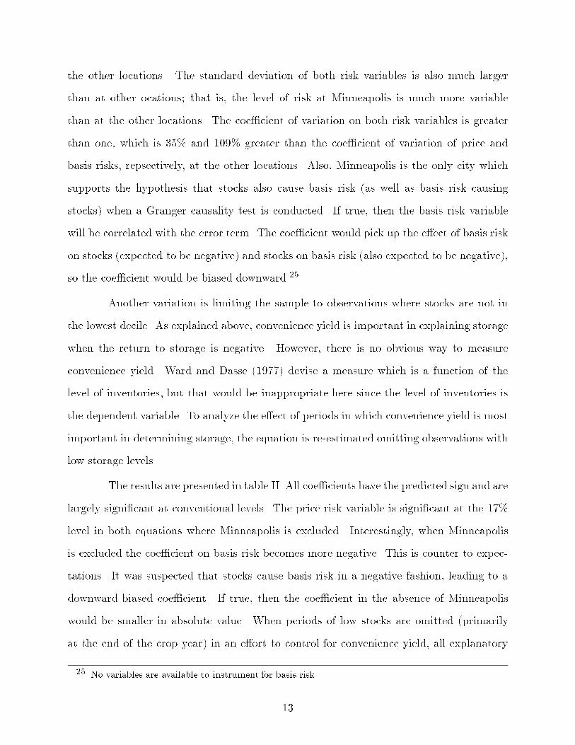
the other locations. The standard deviation of both risk variables is also much larger
than at other ocations; that is, the level of risk at Minneapolis is much more variable
than at the other locations. The coe�cient of variation on both risk variables is greater
than one, which is 35% and 109% greater than the coe�cient of variation of price and
basis risks, repsectively, at the other locations. Also, Minneapolis is the only city which
supports the hypothesis that stocks also cause basis risk (as well as basis risk causing
stocks) when a Granger causality test is conducted. If true, then the basis risk variable
will be correlated with the error term. The coe�cient would pick up the e�ect of basis risk
on stocks (expected to be negative) and stocks on basis risk (also expected to be negative),
so the coe�cient would be biased downward.25
Another variation is limiting the sample to observations where stocks are not in
the lowest decile. As explained above, convenience yield is important in explaining storage
when the return to storage is negative. However, there is no obvious way to measure
convenience yield. Ward and Dasse (1977) devise a measure which is a function of the
level of inventories, but that would be inappropriate here since the level of inventories is
the dependent variable. To analyze the e�ect of periods in which convenience yield is most
important in determining storage, the equation is re-estimated omitting observations with
low storage levels.
The results are presented in table II. All coe�cients have the predicted sign and are
largely signi�cant at conventional levels. The price risk variable is signi�cant at the 17%
level in both equations where Minneapolis is excluded. Interestingly, when Minneapolis
is excluded the coe�cient on basis risk becomes more negative. This is counter to expec-
tations. It was suspected that stocks cause basis risk in a negative fashion, leading to a
downward biased coe�cient. If true, then the coe�cient in the absence of Minneapolis
would be smaller in absolute value. When periods of low stocks are omitted (primarily
at the end of the crop year) in an e�ort to control for convenience yield, all explanatory
25 No variables are available to instrument for basis risk.
13

Table II
Storage
(Standard errors in parentheses)
Independent All Cities,1 No Minneap., All Cities, No Minneap.,Variable All Stocks All Stocks No Low Stocks No Low Stocks
Constant {293.87��� {307.98��� {310.65��� {324.99���
(98.96) (100.49) (107.56) (109.60)
Return 63.29��� 54.49�� 68.57��� 60.73��
(22.05) (21.62) (25.42) (25.85)
Basis Risk {27.63�� {33.75�� {28.53� {37.94��
(14.23) (16.39) (15.42) (18.37)
Price Risk {22.33� {19.42 {25.96� {23.12(13.24) (14.17) (15.36) (16.95)
U.S. Prodn. 37.04��� 39.46��� 41.05��� 43.52���
(13.04) (13.26) (14.28) (14.55)
F 3.43��� 3.12�� 3.18�� 2.95��
D-W 2.06 2.07 2.07 2.08
n 2691 2393 2412 2145
� range {.37 to .54 {.37 to .55 {.39 to .55 {.39 to .55
���Signi�cant at the 1% level. ��Signi�cant at the 5% level. �Signi�cant at the 10% level.1St. Louis, Chicago, Toledo, Gulf, Peoria, Sioux City, Kansas City, Minneapolis, and Omaha-
Council Blu�s
variables have a larger magnitude, by an average of 11%. This is to be expected; in periods
of low levels of inventory, convenience yield will be a dominant in uence.
Interestingly, basis risk is more signi�cant and has a larger impact (see below)
than does price risk. This result might seem counter-intuitive, since the idea is that
agents use futures markets in response to price risk. However, it is precisely the trade-o�
between price and basis risks that explain the result. Working's (1953) hypothesis is that
agents either speculate on the spot price or the basis, whichever is more favorable. When
speculating on the basis, the agent will completely hedge, in which case she will not face
price risk at all. If speculating on the basis occurs more often than speculation on the
spot price, basis risk will be more important than price risk. Alternatively, the portfolio
approach to hedging assumes that agents will form a portfolio of hedged and unhedged
14
stocks. The estimated optimal hedge ratio in the presence of basis risk for corn ranges
from 86% to 98%, depending on when the hedge is lifted relative to the expiration date
(Castelino (1992)). If such a large proportion of the inventory is hedged, the amount that
is subject to price risk is quite small. Thus it would be natural for basis risk to be a
stronger determinant of stocks than price risk.
Table III presents estimates of the magnitude of the e�ect of the independent
variables on storage, which varies across location. Two measures are presented.26;27 One
is the elasticity calculated at the means (in the columns labelled \Elast."). The second
measure gives the percentage of a standard deviation that stocks change when the indi-
cated independent variable increases by one standard deviation (in the columns labelled
\Impact"). That is, when the return to storage increases by one standard deviation in
St. Louis, stocks rise by 13% of a standard deviation.
Storage is elastic with respect to all three independent variables. On average, a 1%
increase in each independent variable causes stocks to change by about .03%. The impact
column gives a more reasonable measure of the magnitude of the e�ect. On average, a one
standard deviation increase in the risk variables causes stocks to increase by over 4% of a
standard deviation, and a one standard deviation increase in the return to storage increases
stocks by over 12% of a standard deviation. The magnitude of the e�ect varies considerably
across locations. Peoria is most sensitive to changes in the independent variables. This
may be explained by the ease with which grain can be moved from Peoria to Chicago or
St. Louis if the economic environment is unfriendly towards storage. The delivery points,
Chicago at par and Toledo at a discount, exhibit the smallest reaction to changes in the
independent variables; delivery may be the largest impact at these locations.28
26 Though the equations are estimated in di�erenced form to control for non-stationarity, the estimatedcoe�cients from the di�erenced form give unbiased estimates of the coe�cients from the level formof the equation. Thus calculations proceed as usual.
27 Calculations use the coe�cients from the sample excluding Minneapolis but including all levels ofstocks. Because the coe�cients do not change substantially across speci�cations, the entries in tableIII are not much changed when other coe�cients are used.
28 Though less than 3% of contracts end in delivery, the average level of stocks in Chicago is less than2500 contracts. In 1992 trade volume for corn was 10.3 million contracts.
15
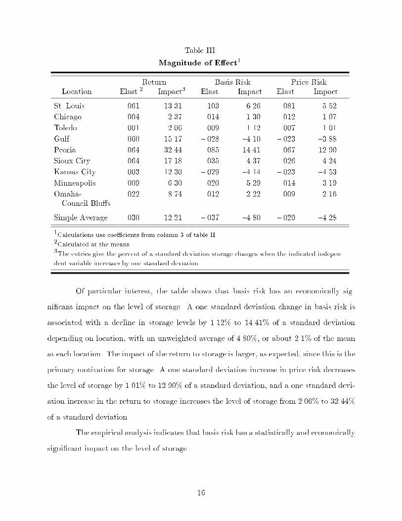
Table III
Magnitude of E�ect1
Return Basis Risk Price Risk
Location Elast.2 Impact3 Elast. Impact Elast. Impact
St. Louis .061 13.31 {.103 {6.26 {.081 {5.52
Chicago .004 2.37 {.014 {1.30 {.012 {1.07
Toledo .001 2.06 {.009 {1.12 {.007 {1.01
Gulf .060 15.17 {.028 {4.10 {.023 {3.88
Peoria .064 32.44 {.085 {14.41 {.067 {12.90
Sioux City .064 17.18 {.035 {4.37 {.026 {4.24
Kansas City .003 12.30 {.029 {4.14 {.023 {4.53
Minneapolis .009 6.30 {.020 {5.29 {.014 {3.19
Omaha- .022 8.74 {.012 {2.22 {.009 {2.16Council Blu�s
Simple Average .030 12.21 {.037 {4.80 {.029 {4.28
1Calculations use coe�cients from column 3 of table II.2Calculated at the means.3The entries give the percent of a standard deviation storage changes when the indicated indepen-
dent variable increases by one standard deviation.
Of particular interest, the table shows that basis risk has an economically sig-
ni�cant impact on the level of storage. A one standard deviation change in basis risk is
associated with a decline in storage levels by 1.12% to 14.41% of a standard deviation
depending on location, with an unweighted average of 4.80%, or about 2.1% of the mean
at each location. The impact of the return to storage is larger, as expected, since this is the
primary motivation for storage. A one standard deviation increase in price risk decreases
the level of storage by 1.01% to 12.90% of a standard deviation, and a one standard devi-
ation increase in the return to storage increases the level of storage from 2.06% to 32.44%
of a standard deviation.
The empirical analysis indicates that basis risk has a statistically and economically
signi�cant impact on the level of storage.
16
VI. Conclusions and Implications
This paper represents the �rst attempt to empirically estimate the e�ect of basis
risk on positions in cash markets. A traditional portfolio model of risk-averse storers is
used to demonstrate that basis risk negatively impacts the level of storage as well as the
hedge ratio. The result that basis risk a�ects the level of storage is then empirically tested
using data on storage of corn in the nine major American markets in the mid-1980s. This
particular test is chosen given data availability.
The model suggests that basis risk negatively a�ects the level of storage, since the
existence of basis risk limits the e�ectiveness of futures as a risk management tool. As
agents face more basis risk, they reduce their exposure by reducing the level of inventory.
A one standard deviation increase in basis risk is associated with a decline in storage by
between 1% and 14% of a standard deviation, depending on the location, or on average
2.1% of the mean.
While this particular empirical test is of storage, the models presented and dis-
cussed show that basis risk will a�ect the cash market position in all hedging situations
by risk-averse agents. Thus basis risk may a�ect positions in agriculture, petroleum, and
any international transaction where agents use currency futures to hedge against exchange
rate risk. For example, basis risk (and exchange rate risk) places foreign agents at a disad-
vantage when using futures markets in another country. Netz (1992) shows that because
foreign wheat agents face basis risk and exchange rate risk, American agents have an ad-
vantage in storage over foreign agents; thus foreign countries export rather than store a
larger proportion of supply shocks.
17

References
Anderson, Ronald W. and Jean-Pierre Danthine. (1981):\Cross-Hedging," Journal of Po-
litical Economy, 89:1182{96.
Brennan, Michael J. (1958):\The Supply of Storage," American Economic Review , 48:pp.50{72.
Castelino, Mark G. (1992):\Hedge E�ectiveness: Basis Risk and Minimum-Variance Hedg-
ing," Journal of Futures Markets, 12:pp. 187-201.
Crop Reporting Board. (January 1981 to December 1989):Crop Production, Washington,DC: United States Department of Agriculture.
Economic Research Service. (March 1993):Feed Situation and Outlook Yearbook, Washing-ton, DC: United States Department of Agriculture.
Ederington, Louis H. (1979):\The Hedging Performance of the New Futures Markets," TheJournal of Finance, 34:pp. 157{70.
Ehrhardt, Michael C., James V. Jordan and Ralph A. Walkling. (1987):\An Applicationof Arbitrage Pricing Theory to Futures Markets: Tests of Normal Backwardation,"Journal of Futures Markets, 7:21{34.
Figlewski, Stephen. (1984):\Hedging Performance and Basis Risk in Stock Index Futures,"The Journal of Finance, 39:pp. 657-69.
Fuller, Wayne A. (1976):Introduction to Statistical Time Series. New York: Wiley.
Garcia, Philip, Raymond M. Leuthold, and Mohamed E. Sarhan. (1984):\Basis Risk:
Measurement and Analysis of Basis Fluctuations for Selected Livestock Markets,"American Journal of Agricultural Economics, 66:pp. 499-504.
Kaldor, Nicholas. (1939):\Speculation and Economic Stability," The Review of Economic
Studies, 7:1{27.
Kenen, Peter and Dani Rodrik. (1986):\Measuring and Analyzing the E�ects of Short-term Volatility in Real Exchange Rates," Review of Economics and Statistics, 68:pp.311-5.
Kmenta, Jan. (1986):Elements of Econometrics, New York:Macmillan Publishing Com-pany.
18
Kolb, Robert W. (1992):\Is Normal Backwardation Normal?," Journal of Futures Markets,
12:75{91.
Livestock and Grain Market News Branch. (January 1981 to December 1989):Stocks of
Grain at Selected Terminal and Elevator Sites, Washington, DC: United States De-
partment of Agriculture.
Martin, Larry, John L. Groenewegen, and Edward Pidgeon. (1980):\Factors A�ecting
Corn Basis in Southwestern Ontario," American Journal of Agricultural Economics,
62:pp. 107-12.
Moser, James T. and Billy Helms. (1990):\An Examination of Basis Risk Due to Estima-
tion," Journal of Futures Markets, 10:pp. 457{67.
Netz, Janet S. (1992):\Basis and Exchange Rate Risks and Their Impact on Storage andExports," working paper.
. (1994):\The E�ect of Futures Markets and Corners on Storage and SpotPrice Variability," American Journal of Agricultural Economics, forthcoming.
Paroush, Jacob and Avnar Wolf. (1992):\The Derived Demand with Hedging Cost Uncer-tainty in the Futures Markets," The Economic Journal , 102:pp. 831{44.
. (1989):\Production and Hedging Decisions in the Presence of Basis Risk,"Journal of Futures Markets, 9:547{63.
Peck, Anne E. (1975):\Hedging and Income Stability: Concepts, Implications, and anExample," American Journal of Agricultural Economics, 57:pp.410{419.
Plosser, Charles I. and G. William Schwert. (1978):\Money, Income, and Sunspots: Mea-suring the Economic Relationships and the E�ects of Di�erencing," Journal of Mon-
etary Economics, 4:637{60.
Stein, Jerome L. (1961):\The Simultaneous Determination of Spot and Futures Prices,"American Economic Review , 51:pp. 1012{25.
Telser, Lester G. (1958):\Futures Trading and the Storage of Cotton and Wheat," Journalof Political Economy, 66:233{55.
Teigen, Lloyd D. (1992):Weather in U.S. Agriculture, computer �le #92008B, WashingtonDC: Economic Research Service, U.S. Department of Agriculture.
Tilley, Daniel S. and Steven K. Campbell. (1988):\Performance of the Weekly Gulf-Kansas
City Hard-Red Winter Wheat Basis," American Journal of Agricultural Economics,
70:929{35.
19

Turnovsky, Stephen J. (1983):\The Determination of Spot and Futures Prices with Storable
Commodities," Econometrica, 51:pp. 1363-87.
Vollink, William and Ronald Raikes. (1977):\An Analysis of Delivery-Period Basis Deter-
mination for Live Cattle," Southern Journal of Agricultural Economics, 9:179{84.
Ward, Ronald W. and Frank A. Dasse. (1977):\Empirical Contributions to Basis Theory:
The Case of Citrus Futures," American Journal of Agricultural Economics, 59:pp.
71{80.
Williams, Je�rey. (1986):The Economic Function of Futures Markets. Cambridge: Cam-bridge University Press.
Working, Holbrook. (1949):\The Theory of Price of Storage," American Economic Review ,39:pp. 1254-62.
Working, Holbrook. (1953):\Hedging Reconsidered," Journal of Farm Economics, 35:pp.544-61.
20


