Page 1
An empirical test of the environmental Kuznets curve:
The effects of industry and trade
by Juan I. Senisterra
ID: 7258157
Major Paper presented to the
Department of Economics of the University of Ottawa
in partial fulfillment of the requirements of the M.A. Degree
Supervisor: Professor Anthony Heyes
ECO 6999
Ottawa, Ontario
August 2017
Page 2
1
The last quarter of the 20th
century saw a growing awareness of the need for
environmental protection. Indeed, modern environmentalism has developed largely in response
to the perceived threat that economic growth has on the Earth’s natural systems. One of the first
publications to bring attention to the sustainability problem was the 1972 book The Limits to
Growth (and subsequent updates in 1992 and 2004). In it, the authors claim that
if the present growth trends in world population, industrialization, pollution, food production and resource
depletion continue unchanged, the limits to growth on this planet will be reached sometime within the next
100 years. The most probable result will be a sudden and uncontrollable decline in both population and
industrial capacity.
Meadows et al. (1992), p. xiii
There was particular concern that many of the world’s rapidly industrializing nations – especially
China and India, which together account for about one third of the global population – would not
be able to reap the benefits of sustained economic growth without causing severe environmental
destruction. It was widely believed that an increase in a nation’s per capita income would have a
positive effect on per capita environmental degradation.
However, by the early 1990s this assumption that continued economic growth would
cause ever increasing environmental decay came under question. The World Development Report
1992 noted that “The view that greater economic activity inevitably hurts the environment is
based on static assumptions about technology, tastes and environmental investments” (World
Bank, 1992, p. 38). It was suggested by some economists that the relationship between economic
growth and environmental damage followed an inverted U shape. With respect to air and water
pollution the idea was that an increase in per capita income would result in higher emissions per
capita until per capita income reaches a turning point, after which a continued rise in income
Page 3
2
would actually reduce emissions per capita (Perman et al., 2011). This relationship came to be
known as the environmental Kuznets curve (EKC).
General overview of the EKC
The basic shape of the environmental Kuznets curve (EKC) is illustrated by the following
figure.
The graph of the EKC shows that in the early stages of economic development, an increase in
individual income contributes to greater degradation per capita. This increasing relationship
continues until a certain level of development is reached (the turning point). Continued economic
growth after this point leads to a reduction in per capita environmental degradation. The dotted
Figure 1. Theoretical relationship between degradation per
capita and income per capita in the EKC
Page 4
3
portion of the curve indicates uncertainty over whether or not degradation per capita eventually
falls back down to 0 for high enough income. The EKC hypothesis is explained as follows:
At low levels of development both the quantity and intensity of environmental degradation is limited to the
impacts of subsistence economic activity on the resource base and to limited quantities of biodegradable
wastes. As economic development accelerates with the intensification of agriculture and other resource
extraction and the takeoff of industrialisation, the rates of resource depletion begin to exceed the rates of
resource regeneration, and waste generation increases in quantity and toxicity. At higher levels of
development, structural change towards information-intensive industries and services, coupled with increased
environmental regulations, better technology and higher environmental expenditures, result in levelling off
and gradual decline of environmental degradation.
Panayotou (1993)
As a result, many economists have argued that if the EKC relationship were to hold true, then
economic growth provides a solution (and not a threat) for improving environmental quality. As
Beckerman (1992) notes, “the best – and probably the only – way to attain a decent environment
in most countries is to become rich.”
Indicators of environmental quality and income:
Before we continue our discussion of the EKC, it is necessary to describe various
indicators of environmental degradation. The most common are pollutants that are by-products
of economic production and consumption. Examples include air pollutants such as carbon
dioxide (CO2), methane (CH4), nitrous oxide (N2O), carbon monoxide (CO), sulphur dioxide
(SO2), fluorinated gases, volatile organic compounds, as well as suspended particulates like
black carbon smoke. Water pollutants, such as nitrates and phosphorous, are also often used.
Page 5
4
Other common indicators of water quality are biological oxygen demand and levels of dissolved
oxygen. Some studies have also used lack of clean water, lack of urban sanitation, annual
deforestation rates, agricultural land fertility, municipal waste, and levels of bacteria in water.
With respect to air and water pollutants, it is important to note that the indicators may be
taken as either emissions (typically measured in tonnes) or ambient concentrations (typically
measured in micrograms per cubic metre, or in parts per million). All levels are usually taken as
annual measurements, and all are reduced to per capita terms.
Finally, the other variable in the EKC relationship is income. It is usually measured by
gross domestic product (GDP). It may be adjusted across countries according to either
purchasing power parity or market exchange rates (usually in terms of US dollars for a chosen
base year).
Causes and Effects:
We now turn our attention to discuss the economic factors that may be responsible for the
EKC relationship between income and environmental degradation. Much of the discussion
follows the analysis from David Stern’s (2004) paper “The Rise and Fall of the Environmental
Kuznets Curve”.
Stern (2004) identifies both scale effects and time effects. The scale effect describes the
growth in pollution and other environmental impacts that would be caused by pure growth in the
scale of the economy if we assumed no structural or technological changes in the economy. The
time effects are independent of income and describe the reduction in environmental impacts
Page 6
5
observed in countries at all levels of income as time progresses. One possible explanation for the
EKC effect, as Stern (2004) suggests, is that middle-income countries experience rapid growth
such that the scale effect, with its accompanying increases in environmental degradation,
overwhelms the time effect. Conversely, wealthy countries experience slower growth such that
the time effect (associated with pollution reduction efforts and improved technologies)
overcomes the scale effect.
Stern also identifies both proximate causes and underlying causes that may explain the
EKC. The underlying causes are those such as environmental regulation, awareness, and
education, which influence the EKC only through proximate variables. The proximate causes are
listed as follows:
Scale of production refers to industrial input-output flow for given factor-input ratios,
output mix, and state of technology. Every 1% increase in scale is assumed to increase
emissions by 1%, ceteris paribus.
Pollution intensities refers to the different output mixes characteristic of different
industries. As industries change over the course of economic development – for example,
from agriculture to manufacturing to services – the output mix (and emissions per unit of
output) changes accordingly. A service industry typically pollutes less than a heavy
manufacturing one.
Changes in input mix refers to substitution of inputs that are more environmentally
damaging for inputs that are less damaging, and vice versa. Other things equal, this
change holds output constant.
State of technology. As technology improves, industries benefit from the increased
productivity of existing processes. More output can be produced with fewer inputs.
Page 7
6
Lower emissions per unit of output can also be achieved. Alternatively, new technologies
may change production processes altogether so that they use less inputs per unit of output
and less emissions per unit of output. In the case of deforestation, for example, better
scientific knowledge and technology may suggest more replanting, selective cutting, and
wood recovery such that less deforestation is required per unit of wood produced.
As mentioned, any observed changes in the level of pollution must be caused by changes in the
proximate variables. However, it must be noted that those changes in proximate variables may be
driven by corresponding changes in underlying variables. For example, over the course of
economic development, preferences and cultural changes may induce corresponding changes in
proximate variables that result in reduced emissions.
Econometric structure:
As the EKC is essentially an empirical phenomenon, an econometric approach is
necessary to describe and test the relationship using our observations. The most basic EKC
regression equation is given by
ln 𝐸𝑖𝑡 = 𝛾 + 𝐹𝑖 + 𝐾𝑡 + 𝛿 ln 𝑌𝑖𝑡 + 𝜙 (ln 𝑌𝑖𝑡)2 + 휀𝑖𝑡 (1)
where E is emissions per capita; Y is income per capita; F represents country-specific effects; K
represents time-specific effects; ε is the random error; γ, δ, and ϕ, are regression parameters; and
i and t are country and time indicators, respectively. The logarithm of Y is used to model the
relationship in order to impose the restriction that the indicators be positive, i.e. Y > 0 and E > 0.
Since the logarithm is a strictly monotone increasing function, the value of Y at which E is
Page 8
7
maximized is the same value at which ln E is maximized. Thus, the value of income Y at which
the indicator for environmental degradation E is at a maximum is given by
𝑌∗ = exp(-δ/(2ϕ))
This is the so-called ‘turning point’ of the environmental Kuznets curve – the income level up to
which emissions are increasing and beyond which emissions decline. Implicit in the EKC
equation is the assumption that the income elasticity is constant across countries at a given
income level, even though emissions per capita may vary across countries at any particular
income level.
The above model is usually estimated using panel data, i.e. pooled cross-sectional time-
series data. The cross-sectional units, indicated by the subscript i, are typically countries or
regions. The subscript t indicates the time period, usually the calendar year. The term Kt in
equation (1) above is used to account for possible time-varying omitted variables and stochastic
shocks that are experienced by all countries. The model itself is most often estimated using either
fixed-effects or random-effects. In the fixed-effects model, the terms Fi and Kt are treated as
regression parameters. The random-effects model, on the other hand, considers Fi and Kt as
components of the random disturbance εit. As Stern (2004) points out, in general, the fixed-
effects model can be estimated consistently. We can use a Hausman test to compare the slope
parameters calculated by both the fixed-effects and random-effects models. If the difference is
statistically significant, then the random-effects model is estimated inconsistently because of the
correlation between the explanatory variables and the error εit.
Even though the fixed-effects model can be estimated consistently, an important point to
keep in mind is that the parameters estimated are conditional on the country and year in the data
Page 9
8
sample. Consequently, it would be inappropriate to use our estimated model to extrapolate to
other samples of data. In particular, if only developed country data are used to estimate our
fixed-effects model, then it may not be of much use to describe the future behaviour of
developing countries (Stern, 2004).
Although many environmental economists take the EKC as a stylized fact, the question of
whether the relationship can be generalized for all classes of pollutants and measurements is a
matter to be tested. According to Stern (2004), the EKC may be valid for local concentrations of
certain pollutants. However, recent evidence suggests that the relationship for emissions may
well be monotonic. In such a case, the inverted U-shaped curve would not be a desirable property
for the econometric model.
Findings from previous studies:
Many early studies indicate that the inverted U-shape of the EKC is a property more
characteristic of local pollutants rather than global ones (Stern, 2004). As theory suggests, local
impacts affect individual regions internally and will likely encourage environmental policies to
correct for them before they are applied to global problems.
With respect to the measures of environmental degradation and income, Stern et al.
(1996) found higher turning points for the EKC when purchasing power parity adjusted income
was used instead of market exchange rates and when emissions of pollutants were used instead
of ambient concentrations in urban areas. In other words, using ambient concentrations of
pollutants will likely produce an EKC relationship with a more evident and narrower inverted U-
shape. One possible explanation for why ambient concentrations may increase and decrease
Page 10
9
more quickly with income is that in the early stages of economic development industrial activity
is usually concentrated in small areas with high population densities. With further economic
development, industries tend to spread outward and cities’ high population densities gradually
decrease through the process of suburbanization (Stern, 2004). These observations are consistent
with Selden and Song’s (1994) study in which they used panel data from developed countries to
estimate EKCs for four different air pollutants. They found that the turning point in the EKC for
emissions was higher than that for ambient concentrations. Furthermore, as Stern (2004) points
out, “it is possible for peak ambient pollution concentrations to fall as income rises even if total
national emissions are rising.”
Another influential EKC study is Grossman and Krueger’s (1991) study on the potential
effects of NAFTA. They used a panel data set of ambient concentrations from several cities
around the world. The pollutants measured were SO2, dark matter, and suspended particles. For
each one, the per capita concentrations were regressed as a cubic function of purchasing power
parity GDP per capita together with various site-related variables, a time trend, and a trade
intensity variable. What they found was an N-shaped curve for SO2 and dark matter with
concentrations increasing, decreasing, and then increasing again. The first turning point occurred
at around $4000 – 5000. For income levels over $10,000 – 15,000, the concentrations of
pollutants appeared to increase once again.
Shafik and Bandyopadhyay’s (1992) study used a similar analysis to estimate EKCs for
different indicators of environmental quality. They concluded that lack of clean water and lack of
urban sanitation decrease monotonically with rising income. On the other hand, river quality
deteriorated with income. Two of the air pollutants measured seemed to support the EKC
hypothesis with both having turning points at income levels in the $3000 – 4000 range.
Page 11
10
However, municipal waste and carbon emissions were found to increase monotonically with
increasing income.
Emissions based estimates such as those of Selden and Song’s (1994) study used data that
is primarily from OECD countries. As a result, the values of income per capita in the sample are
fairly high and with relatively small variability among them. According to Stern (2004), using a
larger sample that includes data from more low-income countries might result in an EKC turning
point that is higher. In fact, Stern and Common (2001) used emissions of sulphur data from the
US Department of Energy that covered a large range of income per capita and found the
estimated turning point at over $100,000! Stern (2004) claims that more recent studies using
larger representative samples show that both sulphur and carbon dioxide emissions increase
monotonically with rising income.
Altogether, Stern (2004) suggests that the particular choice of sample used is at least
partly responsible for the differences in turning points seen for different pollutants. Comparing
various studies, the overall impression is that concentrations of pollutants may exhibit the
inverted U-shape, rising and then falling, with the peak (turning point) corresponding to middle-
income countries. By contrast, emissions tend to increase monotonically with income.
Weaknesses in the EKC theory:
One of the main criticisms of the EKC theory strikes at the heart of the model itself in
that it takes income as the independent variable and environmental degradation as the dependent
one. According to Arrow et al. (1995) and Stern (2004), the model assumes that “environmental
damage does not reduce economic activity sufficiently to stop the growth process and that any
Page 12
11
irreversibility is not so severe that it reduces the level of income in the future” (Stern, 2004). In
other words, income is taken as exogenous and there is assumed to be no feedback from
environmental damage to economic production. In short, the EKC model assumes that the
economy is sustainable. However, if environmental damage erodes the productivity of an
economy, then persistent growth – particularly in the early stages of development – may turn out
to be ‘uneconomic’.
Another common weakness of most early EKC literature is its failure to consider the
relationships between different pollutants and the possible substitution of one for the other. Over
the course of economic development, new technologies often alter industrial processes by
changing the composition of inputs and outputs. Therefore, it is possible for one pollutant to be
gradually replaced by another. While the former may possess the inverted U characteristic over
the course of economic growth, the latter may not. As a result, the efforts to reduce some impacts
may worsen others (Stern, 2004).
Finally, another argument suggests that if there is an apparent EKC relationship between
income and pollution, it may be due to the effects of trade on the distribution of polluting
industries around the world (Stern, 2004). There are at least two possible explanations for this
phenomenon:
First, as trade theory suggests, countries tend to specialize “in the production of goods
that are intensive in the factors that they are endowed with in relative abundance” (Stern,
2004). Consequently, developing countries would specialize in activities such as
harvesting, processing raw materials, and heavy manufacturing that are intensive in
labour and natural resources. Meanwhile, the developed countries would specialize in
Page 13
12
services and lighter manufacturing which are intensive in human capital and physical
capital already in place. The low levels of environmental degradation experienced by
high-income countries and the corresponding higher levels in middle-income countries
may result from such specializations (Stern, 2004).
Second, environmental regulations in developed countries may encourage polluting
industries to relocate their activities to developing countries (Stern, 2004). This
redistribution of polluting activities may explain the apparent shape of the EKC. Since we
live in a finite world with a limited number of countries and regions, as poor countries
become wealthy they will eventually be “unable to find further countries from which to
import resource intensive products” (Stern, 2004). As a result, if these countries wish to
introduce similar environmental regulations as the developed countries, they would have
no choice but to abate polluting activities rather than outsource them (Arrow et al., 1995).
We will look at the effects of trade more closely in the next section.
Trade and the Pollution Haven Hypothesis
We now turn to examine the extent to which trade and industry may explain the
relationship between per capita income and pollution in the environmental Kuznets curve. In
principle, it is possible for high income economies to specialize in the production of ‘clean’
goods and services while low (or middle) income economies specialize in the production of
‘dirty’ ones. The result would be that high income economies would experience a reduction in
per capita pollution even though they are relying and depending on products originating in lower
income economies. This effect is known as the pollution haven hypothesis (PHH). The most
Page 14
13
important consequence of this phenomenon is that the EKC would imply not an overall reduction
in pollution but rather a transfer of pollution from high income countries to lower income ones.
The relationship between trade and the environment may be described by three
independent effects (Grossman and Krueger, 1991; Cole, 2004).
The scale effect describes the likely increase in pollution caused by economic growth
resulting from increased market access due to trade.
The technique effect refers to a change in the production process that may result from free
trade. These may be induced by a demand for greater environmental regulations and the
adoption of more environmentally-friendly production technologies.
The composition effect refers to changes in the composition of an economy that may
result from trade as countries increasingly specialize in production for which they have a
comparative advantage.
The composition effect is the one that is most relevant to the environmental Kuznets curve and
serves as the mechanism through which the PHH would affect pollution.
Historically, as industrial economies have developed, there has been a change in
composition from heavy industry towards lighter manufacturing and services. Developing
economies, on the other hand, have become more specialized in the heavy industrial sectors
(Cole, 2004). These structural changes may be captured by including the ratio of manufactured
exports to domestic manufacturing production as an independent variable in the EKC. Similarly,
this ratio may be calculated using imports instead of exports. If we find that the export ratio has a
positive relationship with pollution, or that the import one has a negative relationship, then it
may count as evidence in support of the PHH, in which case some countries specialize in the
Page 15
14
production of ‘dirty’ goods while others specialize in ‘clean’ goods (Stern, 2004). Furthermore,
if these structural changes also coincide with the middle-income countries taking on dirty
production and high-income countries specializing in clean products, then it may explain the
inverted U relationship of the EKC. Thus, the claim that economic growth provides a ‘cure’ for
environmental problems would be seriously undermined because as income increases, developed
countries would simply export their ‘dirty’ industries to middle-income developing countries. If
this is indeed the case, then there will come a time when developing countries have no one on
whom to pass their pollution-intensive industries. It would be impossible for them to follow the
same pollution-income path that today’s developed economies have been able to experience.
If it is true that countries specialize according to their relative abundance of factors of
production, then we would expect the developed (high-income) countries to increase its
specialization in capital intensive industries while the developing (low and middle-income)
countries specialize in labour intensive ones. Capital intensive sectors are usually more
pollution-intensive than the labour intensive ones. Nevertheless, previous studies have suggested
that the capital intensive sectors tend to be dirtier than the labour intensive ones (Cole, 2004).
Under this line of reasoning, it would not be at all obvious that factor abundance explains the
shape of the EKC.
One explanation of why pollution havens may exist in the first place is the possible
difference in environmental regulations between developed (high income) and developing (low
to middle income) countries. As the developed world implements more stringent environmental
regulations and the costs of complying with them increases, industrial activities that are
Page 16
15
pollution-intensive may relocate to developing countries that have fewer regulations. In other
words, “developing countries may have a comparative advantage in pollution-intensive
production.” (Cole 2004)
However, the evidence for low-regulation pollution havens is somewhat mixed. Some
studies find no evidence, whereas others find evidence for temporary pollution havens. Mani and
Wheeler (1998) support this last theory with their analysis of dirty industries’ import-export
ratios. Also, Lucas et al. (1992), and Birdsall and Wheeler (1993) suggest that an increase in
pollution intensity in developing countries corresponds to periods of tougher OECD
environmental regulations. Other studies, such as Antweiler et al. (2001), analyzed how the
concentration of sulfur dioxide at city level was impacted by trade liberalization, as evidence of
“pollution haven pressures.” Adding to the mixed findings, contradicting studies show, at one
end, evidence that trade patterns are influenced by regulations (Van Beers and Van den Bergh,
1997) and at the other end, that this evidence is not accurate when the studies include fixed
effects (Harris et. al, 2002). Furthermore, some analysts–such as Ederington and Minier (2003),
and Levinson and Taylor (2002)—focus on endogeneity arguments, stating that the
environmental regulations influence trade patterns in the US, only when they are considered an
endogenous variable, and therefore they are only “secondary barriers.”
The search for an interpretation of the lack of substantial evidence of pollution havens, in
spite of the theoretical expectations, include arguments related to the real cost of environmental
compliance. Indeed, even though significant in absolute values, these costs amount to a small
percentage (2% or less) of the total costs of the industry, reducing the disadvantaged
competitiveness in highly regulated countries to an insignificant factor (Walter, 1973, 1982;
Tobey, 1990; Dean, 1991). Other approaches to explain the small evidence in favour of the
Page 17
16
pollution havens theory and the relocation of industries include the dependence of heavy
industries on home markets, and the factors of unreliable regulations that deter foreign
investment. Besides, the pollution intensive production has not seen a reduction in absolute
terms, even though its share of GDP shows a decrease.
Thus, in the context of PHH, it is important to evaluate the role of consumption in the
specialization patterns of net exports. Then, the increase of net exports in pollution intensive
sectors in developing countries could be the result of an increase in their domestic consumption
of ‘dirty’ products. Therefore, net exports need to be analyzed as a proportion of consumption,
for trade of ‘dirty’ output for a developed country with a developing one (Cole 2004). This
evaluation would show a reduction in specialization in relation to consumption in a developed
country, and the consequent assumption that the developing countries are supplying the demand
for pollution-intensive products. When the specialization patterns for ‘dirty’ products are
compared between developed and developing regions over time, there is indication of falling
NETXC during specific periods and between particular trading countries, supporting the PHH
theory. However, this decrease in NETXC was also seen in many ‘clean’ industries, when
observing their specialization patterns comparing developed and developing trading regions.
Consequently, these findings imply that the different environmental regulations and compliance
between developed and developing countries are not the only factors to be considered.
Estimating EKCs
In order to include all the considerations studied in the previous analyses of EKC, and
overcome many of their contradicting arguments, Cole (2004) estimates the following EKC
model:
Page 18
17
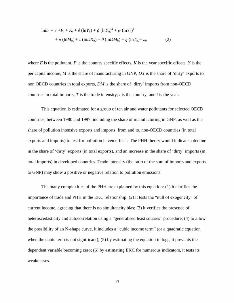
lnEit = 𝛾 +Fi + Kt + δ (lnYit) + ϕ (lnYit)2 + ψ (lnYit)
3
+ σ (lnMit) + λ (lnDXit) + θ (lnDMit) + η (lnTit)+ εit (2)
where E is the pollutant, F is the country specific effects, K is the year specific effects, Y is the
per capita income, M is the share of manufacturing in GNP, DX is the share of ‘dirty’ exports to
non OECD countries in total exports, DM is the share of ‘dirty’ imports from non-OECD
countries in total imports, T is the trade intensity; i is the country, and t is the year.
This equation is estimated for a group of ten air and water pollutants for selected OECD
countries, between 1980 and 1997, including the share of manufacturing in GNP, as well as the
share of pollution intensive exports and imports, from and to, non-OECD countries (in total
exports and imports) to test for pollution haven effects. The PHH theory would indicate a decline
in the share of ‘dirty’ exports (in total exports), and an increase in the share of ‘dirty’ imports (in
total imports) in developed countries. Trade intensity (the ratio of the sum of imports and exports
to GNP) may show a positive or negative relation to pollution emissions.
The many complexities of the PHH are explained by this equation: (1) it clarifies the
importance of trade and PHH in the EKC relationship; (2) it tests the “null of exogeneity” of
current income, agreeing that there is no simultaneity bias; (3) it verifies the presence of
heteroscedasticity and autocorrelation using a “generalised least squares” procedure; (4) to allow
the possibility of an N-shape curve, it includes a “cubic income term” (or a quadratic equation
when the cubic term is not significant); (5) by estimating the equation in logs, it prevents the
dependent variable becoming zero; (6) by estimating EKC for numerous indicators, it tests its
weaknesses.
Page 19
18
When analysing the estimated results for the air pollutants and the water quality
indicators, the World Bank data of various per capita incomes was used to observe the turning
points in context (Cole 2004). For almost all the indicators at significant levels, there is an
inverted U-shape relationship with per capita income, and there is no indication of an N-shape
relationship between per capita income and emissions. In other words, when incomes rise at high
levels, emissions are not increased. Also, the manufacturing share of GNP shows a positive
relationship with environmental quality, indicating that there is a correlation between structural
changes within the economies and the reduction in ‘dirty’ emissions at high levels of income.
Most of the observations of PHH show mixed evidence when considering the share of
‘dirty’ exports in total exports, and the share of ‘dirty’ goods in total imports. Indeed, while there
are indications that the imports from the developing world replace the domestic manufacturing of
intensive-pollution products, the share of ‘dirty’ exports to the developing countries has a
positive impact on environmental quality.
Therefore, these findings cannot fully support the statement that the transfer of ‘dirty’
industry to developing countries has an impact on pollution, and the economic significance is
low.
Some interesting points are drawn from the analysis of the variables of the equation: (1)
the basic EKC may indicate pollution haven effects that contribute to the reduction in emissions
at higher income levels; (2) there is a positive relationship between trade openness and
environmental quality for OECD countries; (3) there is an improvement in environmental quality
over time due to various factors, such as regulations, technology, efficiency, and education.
Page 20
19
The study of the effect of trade through pollution haven effects and structural change on
the EKC relationship carried by Cole (2004) sheds some light on the following issues: although
pollution havens form temporarily and limitedly in some specific regions and sectors, they may
have an effect on pollution emissions. By analyzing the significance played by income, trade
openness, structural changes and ‘dirty’ trade between developed and developing regions on air
and water pollutants, there is indication that there is a relationship between each pollutant and the
per capita income. Also, environmental quality and emissions are partially connected to the share
of pollution intensive imports and exports between OECD and non-OECD countries, albeit not
for all pollutants nor with a significant economic impact.
The study of EKC shows two important conclusions. First, the share of manufacturing
output in GDP has an importantly positive relationship with pollution. Second, trade openness
indicates a negative relationship with pollution, when controlling structural change, income and
PPH effects. Thus, the reduction in emissions at high levels of income could be attributed to
more rigorous environmental regulations, trade openness, structural change to reduce the share of
manufacturing output, increase in imports of pollution-intensive goods. (Cole 2004)
It is still not clear which will be the future behaviour in the demand in the developing
world for manufactured products as a share of GDP. Therefore, unless the income elasticity of
demand for manufactured products drops with income, the decrease in manufacturing share of
GDP in the developed world can only be explained so far by the transferring of manufacture to
the developing world, which will have no escape from this pollution-intensive activity.
Page 21
20
Estimating an EKC
We now turn to estimating an environmental Kuznets curve in a similar fashion to Cole
(2004). Using the World Bank’s “DataBank: World Development Indicators,” we obtain
information for 214 countries (from Afghanistan to Zimbabwe) for each year from 1960 to 2013
and organize it in a cross-sectional time-series (panel data) array. We consider the following
variables:
E is carbon dioxide (CO2) emissions (metric tons per capita); Y is GDP per capita (2013 US
dollars); M is manufacturing product as a percentage of GDP; MI is manufacturing imports as a
percentage of total imports; MX is manufacturing exports as a percentage of total exports; T is
trade as a percentage of GDP. We then transform each of these variables by taking the logarithm
of each, denoting the new variables with lower case letters:
e = log E
y = log Y
m = log M
mi = log MI
mx = log MX
t = log T
We will estimate four models in total: a simple quadratic, an expanded quadratic, a simple cubic,
and an expanded cubic. (The models are quadratic or cubic in income.) The indices i and n will
indicate country and time (year), respectively. (Note that the variable t has been reserved for
trade.) The fixed effects models are estimated in Stata using ordinary least squares (OLS) linear
regression with panel corrected standard errors to account for heteroskedasticity and
Page 22
21
contemporaneous correlation of errors across countries. The variables Fi are the country specific
effects, Kn the year specific effects, and εin the errors. Parameters γ, δ, ϕ, ψ, σ, λ, θ, and η are
those calculated from the data.
The purpose of the quadratic models is to explore the hypothesis that the relationship
between e and y is that of an inverted U-shape. In other words, that increasing income causes an
increase in emissions up to a point, past which further increases in income bring a decrease in
emissions. This is the premise of the environmental Kuznets curve (EKC). The cubic model
allows for the possibility that emissions may begin to increase again at high income levels (i.e.
that the EKC may actually be an N-shaped curve). In each case, a simple and expanded version
of the model is considered in order to observe any differences in the turning point (income level
at which emissions begin to decrease). The variables m, mi, mx, and t are included in each
expanded model to indicate the extent to which manufacturing and trade may affect pollution.
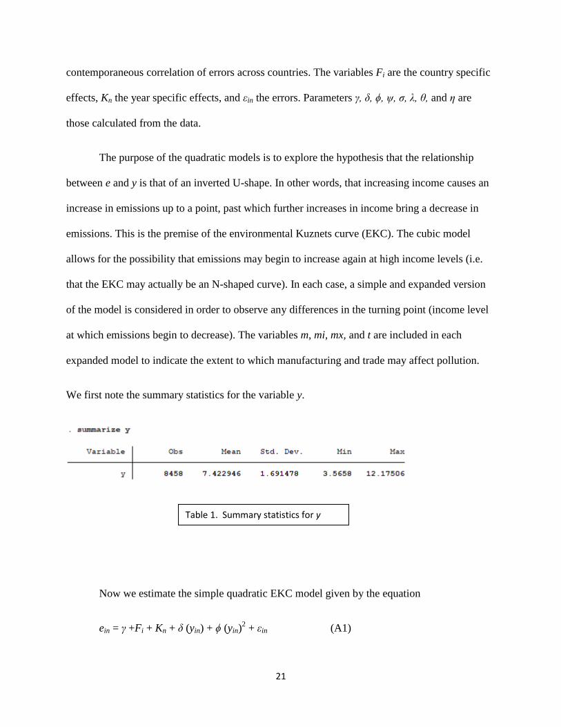
We first note the summary statistics for the variable y.
Now we estimate the simple quadratic EKC model given by the equation
ein = γ +Fi + Kn + δ (yin) + ϕ (yin)2 + εin (A1)
Table 1. Summary statistics for y
Page 23
22
The output in Stata is as follows.
The parameters calculated for equation (A1), including the constant term, are
𝛾 = −4.487609, 𝛿 = 1.521747, �̂� = −0.0761853
The individual p-values of these parameters together with the Wald test suggest the coefficients
are statistically significant.
Next, we test an expanded quadratic model that incorporates manufacturing production,
imports and exports of manufacturing, and trade. Our equation is
Table A1
Page 24
23
ein = γ +Fi + Kn + δ (yin) + ϕ (yin)2 + σ(m)in + λ(mi)in + θ(mx)in + η(t)in + εin (A2)
We obtain the following output from Stata.
The coefficients estimated are
𝛾 = −3.93995, �̂� = 1.020586, �̂� = −.045806, �̂� = 0.2579518,
�̂� = .0551582, 𝜃 = −0.0477342, �̂� = 0.1801219
The p-values and Wald statistic again suggest that these coefficients are significant.
Table A2
Page 25
24
We repeat the procedure, except this time we consider a cubic model of the EKC. We
first estimate the simple cubic.
ein = γ +Fi + Kn + δ (yin) + ϕ (yin)2 + ψ(yin)
3 + εin (B1)
The Stata output is given here:
The coefficients estimated are
𝛾 = −2.214536, 𝛿 = 0.5422632, �̂� = 0.0581466, �̂� = −0.0059135
The p-values and Wald test suggest they are statistically significant.
Table B1
Page 26
25
Finally, we perform an estimate of the expanded cubic model given by the equation
ein = γ +Fi + Kn + δ (yin) + ϕ (yin)2 + ψ(yin)
3 + σ(m)in + λ(mi)in + θ(mx)in + η(t)in + εin
The results from Stata are given as follows.
The parameters are given by
𝛾 = −1.151331 , 𝛿 = −0.1498616, �̂� = 0.1115612 , �̂� = −0.0068283,
�̂� = 0.2500597 , �̂� = 0.047839, 𝜃 = −0.0463718 ,
�̂� = 0.1874767
Table B2
Page 27
26
We can see from the table that the p-value for the coefficient of the y term is quite large.
However, since the coefficients for the y2 and y
3 terms appear statistically significant, we keep all
three in the following analysis. All the other coefficients, together with the Wald test, suggest
that the model is robust.
Analysis
What we wish to examine next is how the turning point of the EKC in the ye-plane is
affected by the additional explanatory variables m, mi, mx, and t.
We begin with the quadratic model. The turning point for both equations (A1) and (A2) is
given by
𝑦∗ = −𝛿
2𝜙
Using the parameters calculated in Tables A1 and A2, we find that the turning points are
y*simple = 9.98714 and y
*expanded = 11.14031
for models A1 and A2, respectively. We may see the differences between these two quadratic
models in the following figure.
Page 28
27
Recalling that y = ln Y, we determine that these turning points correspond to per capita GDP of
$21,745 and $68,893 (in 2013 US dollars), respectively for the simple and expanded models.
Similarly, for the cubic models (B1) and (B2), the turning points are given by
𝑦∗ =−2𝜙−√4𝜙2−12𝛿𝜓
6𝜓
Using the parameters calculated, the turning points are
y*simple = 9.70484 and y
*expanded = 10.17291
for models (B1) and (B2), respectively. The following figure shows the fitted curves for the two
models and their turning points. These values correspond to per capita GDP of $16,397 and
$26,184.
Figure 2. Quadratic models and their turning points. Simple model in solid
line; expanded model in dotted line.
Page 29
28
Mathematically, each of these cubic models ought to have two turning points. Since the lower
turning points occur for very small or even negative values of y, we ignore them as they are
insignificant. We consider only the higher turning points. The results show no considerable
evidence of an N-shaped relationship between y and e.
We do observe in both the quadratic and cubic models that y*simple < y
*expanded. This
observation lends some evidence to the hypothesis that as the EKC model is expanded by
incorporating explanatory variables associated with a potentially “dirty” activity such as
manufacturing and the trade of such products, the turning point at which emissions begin to
decrease occurs at a higher level of income. As such, it remains possible that wealthy countries
may simply be outsourcing pollution-intensive production of goods and services to lower income
countries, thereby lending some validity to the pollution haven hypothesis (PHH).
Figure 3. Cubic models and their turning points. Simple model in solid line;
expanded model in dotted line.
Page 30
29
Discussion
We have examined evidence for the environmental Kuznets curve (EKC) and the
pollution haven hypothesis (PPH). The idea of the EKC appears to be supported by both the
quadratic (A1) and cubic (B1) simple models. Indeed, as countries’ per capita GDP increases,
their per capita emissions of CO2 increase at first, reach a maximum, and then decrease. We then
chose the additional explanatory variables of manufacturing, together with its imports, exports,
and overall trade to see if it would capture some of the effects on emissions. We observed in the
models (A2) and (B2) that the turning points occurred at higher per capita income levels,
certainly not disproving the PHH.
We note that the models were only estimated using only data on emissions of one
particular greenhouse gas (CO2). Furthermore, gross domestic product (GDP) measured in 2013
US dollars was used as the measure of income. It would be interesting to conduct a subsequent
investigation of the EKC and PHH using other measures of environmental degradation as well as
other measures of GDP (such as purchasing power parity).
To grow or not to grow? That is certainly the underlying question motivating any
discussion of the EKC. The significance of the EKC is in giving hope to enthusiasts of economic
growth. It suggests that if all nations become wealthy (and therefore developed) enough, we may
reap the fruits of high levels of consumption (implicit in the definition of “wealthy”) and at the
Page 31
30
same time enjoy a relatively clean environment. The implication is that insufficient development
is the cause of environmental degradation.
To further the discussion, we note the result when we consider global income per capita
and global emissions of CO2 per capita. The variables y and e here denote the logarithms of these
two global measures, respectively.
We see from the figure that there is a fairly strong positive correlation between income per capita
and emissions per capita when observed at the global level. It would appear that as the world gets
wealthier, it also gets dirtier. So what is happening here? It has to be said that environmental
degradation does not respect national boundaries. Whether we are considering the emissions of a
particular greenhouse gas or some other measure, such as deforestation or loss of biodiversity,
Figure 4. Scatter plot of global CO2 emissions per capita and
global income (GDP) per capita. (In logarithms)
Page 32
31
the degradation affects the entire biosphere. We may redraw political boundaries arbitrarily and
consider one such region “clean” and another “dirty” but, to the planet, those distinctions are
meaningless. If we consider the Earth to be one system, the effect of pollution is independent of
which arbitrary region (i.e. “country”) we associate it with. We may engage in as much
environmental gerrymandering as we like, but the relevant measures ought to be global. There is
nothing in Figure 4 to give hope to the belief that as we continue developing and getting
wealthier globally, that we will become cleaner. The cross-sectional (country) unit of analysis in
the EKC is a rather arbitrary measure. There is no reason to believe that there is any universality
to the way societies have drawn their boundaries on a map, let alone that these boundaries are the
ones to consider when examining the effect of human activities on a natural system like the
planet. The EKC’s attempt to study a social phenomenon (such as economic development and
growth) alongside a natural phenomenon (such as environmental impact) is quite reductionist.
As a result, it is very difficult to draw any meaningful conclusions from such an empirical
analysis.
There is also the question of whether GDP is an appropriate measure of human progress
and well-being, and whether indefinite economic growth is desirable. The decision to include
these measures in defining the EKC is the product of an economic ideology that makes several
presumptions – that more material consumption and transactions give us greater freedoms of
“choice” and make us “better off” socially. There is a very utilitarian philosophy implicit in the
EKC. If economic growth is what we are truly interested in, then the EKC does not really answer
the question of whether it can be sustained indefinitely. Different analytic frameworks ought to
be explored to consider the matter further. One such framework is considered in Victor’s (2008)
study, Managing Without Growth: Slower by Design, Not Disaster.
Page 33
32
References
Antweiler, W., Copeland, B. R., Taylor, M. S. (2001). “Is free trade good for the environment?”
American Economic Review 91 (4), 877-908.
Arrow, K., Bolin, B., Costanza, R., Dasgupta, P., Folke, C., Holling, C.S., Jansson, B.-O., Levin,
S., Mäler, K.-G., Perrings, C.A., Pimentel, D. (1995). Economic growth, carrying
capacity, and the environment. Science, 268, 520-521.
Beckerman, W. (1992). Economic growth and the environment: whose growth? Whose
environment? World Development 20, 481-496.
Birdsall, N., Wheeler, D. (1993). “Trade policy and industrial pollution in Latin America: Where
are the pollution havens?” Journal of Environment and Development 2 (1), 137-149.
Cole, M.A. (2004) Trade, the pollution haven hypothesis and the environmental Kuznets curve:
examining the linkages. Ecological Economics 48, 71-81.
Dean, J. (1991). “Trade and the environment: A Survey of the Literature,” Background paper
prepared for the 1992 World Development Report, World Bank.
Ederington, J. Minier, J. (2003). Is environmental policy a secondary trade barrier? An empirical
analysis. Canadian Journal of Economics 36, 137-154.
Grossman, G.M., Krueger, A.B. (1991). Environmental impacts of a North American Free Trade
Agreement. National Bureau of Economic Research Working Paper 3914, NBER,
Cambridge Massachusetts.
Harris, M.N., Konya, L., Matyas, L. (2002). “Modelling the impact of environmental regulation
on bilateral trade flows: OeCD, 1990-96.” World Economy 25 (3), 387-405.
Levinson, A., Taylor, M.S. (2002). Trade and the environment: unmasking the pollution haven
hypothesis. Mimeo, University of Georgetown.
Lucas, R.E.B., Wheeler, D., Hettige, H. (1992). “Economic development, environmental
regulation and the international migration of toxic industrial pollution: 1960-1988.” In:
Low. P. (Ed.), International Trade and the Environment. World Bank Discussion Paper
No. 159.
Meadows, D.H., Meadows, D.L., Randers, J. (1992). Beyond the Limits: Global Collapse or a
Sustainable Future. Earthscan, London.
Page 34
33
Mani, M., Wheeler. D. (1998). “In search of pollution havens? Dirty industry in the world
economy, 1960-1995.” Journal of Environment and Development. 7 (3), 215-247.
Meadows, D.H., Meadows, D.L., Randers, J., Behrens, W.W. (1972). The Limits to Growth: A
Report for The Club of Rome’s project on the Predicament of Mankind. Earth Island,
Universe Books, New York.
Meadows, D., Randers, J., Meadows, D. (2004). Limits to Growth: The 30-Year Update. Chelsea
Green Publishing Company, White River Junction, Vermont.
Panayotou, T. (1993). Empirical Tests and Policy Analysis of Environmental Degradation at
Different Stages of Economic Development. Working Paper WP238, Technology and
Employment Programme, International Labor Office, Geneva.
Perman, R., Ma, Y., Common, M., Maddison, D., McGilvray, J. (2011). Natural Resource and
Environmental Economics. Pearson Education Limited, Harlow, England.
Selden, T.M., Song, D. (1994). Environmental quality and development: Is there a Kuznets curve
for air pollution? Journal of Environmental Economics and Management, 27, 147-162.
Shafik, N., Bandyopadhyay, S. (1992). Economic Growth and Environmental Quality: Time
Series and Cross-Country Evidence. Background Paper for the World Development
Report 1992, The World Bank, Washington, DC.
Stern, D.I. (2004). The Rise and Fall of the Environmental Kuznets Curve. World Development
32 (8), 1419-1439.
Stern, D.I., Common, M.S. (2001). Is there an environmental Kuznets curve for sulfur? Journal
of Environmental Economics and Management, 41, 162-178.
Stern, D.I., Common, M.S., Barbier, E.B. (1996). Economic growth and environmental
degradation: The environmental Kuznets curve and sustainable development. World
Development 24, 1151-1160.
The World Bank. “DataBank: World Development Indicators.”
http://databank.worldbank.org/data/reports.aspx?source=world-development-indicators#
Tobey, J. (1990). “The effects of domestic environmental policies on patterns of world trade: an
empirical test.” Kyklos 43 (2), 191-209.
Van Beers, C., Van den Bergh, J.C.J.M. (1997). “An empirical multi-country analysis of the
impact of environmental regulations on foreign trade flows.” Kyklos 50 (1), 29-46.
Victor, P.A. (2008). Managing Without Growth: Slower by Design, Not Disaster. Edward Elgar
Publishing Limited, Cheltenham, England.
Page 35
34
Walter, I. (1973). “The pollution content of American trade.” Western Economic Journal 9, 1.
Walter I. (1982). Environmentally induced industrial relocation to developing countries. In:
Rubin, S. (Ed.), Environment and Trade. Allanheld, Osmun and Co., New Jersey.
World Bank (1992). World Development Report 1992. International Bank for Reconstruction and
Development, Washington, D.C.
Page 36
35
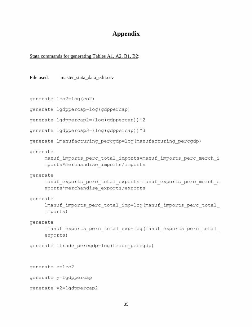
Appendix
Stata commands for generating Tables A1, A2, B1, B2:
File used: master_stata_data_edit.csv
generate lco2=log(co2)
generate lgdppercap=log(gdppercap)
generate lgdppercap2=(log(gdppercap))^2
generate lgdppercap3=(log(gdppercap))^3
generate lmanufacturing_percgdp=log(manufacturing_percgdp)
generate
manuf_imports_perc_total_imports=manuf_imports_perc_merch_i
mports*merchandise_imports/imports
generate
manuf_exports_perc_total_exports=manuf_exports_perc_merch_e
xports*merchandise_exports/exports
generate
lmanuf_imports_perc_total_imp=log(manuf_imports_perc_total_
imports)
generate
lmanuf_exports_perc_total_exp=log(manuf_exports_perc_total_
exports)
generate ltrade_percgdp=log(trade_percgdp)
generate e=lco2
generate y=lgdppercap
generate y2=lgdppercap2
Page 37
36
generate y3=lgdppercap3
generate m=lmanufacturing_percgdp
generate mi=lmanuf_imports_perc_total_imp
generate mx=lmanuf_exports_perc_total_exp
generate t=ltrade_percgdp
encode countrycode, gen(countrycode1)
xtset countrycode1 year
summarize y
xtpcse e y y2 i.countrycode1, pairwise
xtpcse e y y2 y3 i.countrycode1, pairwise
xtpcse e y y2 m mi mx t i.countrycode1, pairwise
xtpcse e y y2 y3 m mi mx t i.countrycode1, pairwise
Stata commands for generating Figure 4:
File used: time_series_aggregate2.csv
generate lgdp=log(gdp)
generate lgdppercap=log(gdppercap)
generate lco2=log(co2_total)
Page 38
37
generate lco2_percap=log(co2_percapita)
generate e=lco2_percap
generate y=lgdppercap
scatter e y
twoway(scatter e y)(lfit e y)
reg e y