An Equilibrium Analysis of Real Estate Leases Steven R. Grenadier ¤ Graduate School of Business Stanford University June 2002 This article provides a uni…ed equilibrium approach to valuing a wide variety of commercial real estate lease contracts. Using a game-theoretic variant of real options analysis, the underlying real estate asset market is modeled as a continuous-time Nash equilibrium in which developers make construction decisions under demand uncertainty. Then, using the economic notion that leasing simply represents the purchase of the use of the asset over a speci…ed time frame, I use a contingent-claims approach to value many of the most common real estate leasing arrangements. In particular, the model provides closed-form solutions for the equilibrium valuation of leases with options to purchase, pre-leasing, gross and net leases, leases with cancellation options, ground leases, escalation clauses, lease concessions and sale-leasebacks. ¤ I thank Geert Bekaert, Bin Gao, Michael Harrison, Harrison Hong, Chester Spatt, Je¤ Zwiebel and seminar particpants at the 2002 AFA meetings, 2002 WFA meetings, Carnegie Mellon, Columbia University, Rochester, Wharton, UCLA and USC for help- ful comments. Correspondence can be addressed to Steven Grenadier, Graduate School of Business, Stanford University, Stanford, CA 94305. Phone: (650) 725-0706, E-mail: [email protected].
Transcript
An Equilibrium Analysis of Real EstateLeases
Steven R. Grenadier¤
Graduate School of BusinessStanford University
June 2002
This article provides a uni…ed equilibrium approach to valuing a wide variety ofcommercial real estate lease contracts. Using a game-theoretic variant of realoptions analysis, the underlying real estate asset market is modeled as acontinuous-time Nash equilibrium in which developers make constructiondecisions under demand uncertainty. Then, using the economic notion thatleasing simply represents the purchase of the use of the asset over a speci…edtime frame, I use a contingent-claims approach to value many of the mostcommon real estate leasing arrangements. In particular, the model providesclosed-form solutions for the equilibrium valuation of leases with options topurchase, pre-leasing, gross and net leases, leases with cancellation options,ground leases, escalation clauses, lease concessions and sale-leasebacks.
¤I thank Geert Bekaert, Bin Gao, Michael Harrison, Harrison Hong, Chester Spatt,Je¤ Zwiebel and seminar particpants at the 2002 AFA meetings, 2002 WFA meetings,Carnegie Mellon, Columbia University, Rochester, Wharton, UCLA and USC for help-ful comments. Correspondence can be addressed to Steven Grenadier, Graduate Schoolof Business, Stanford University, Stanford, CA 94305. Phone: (650) 725-0706, E-mail:[email protected].
1 IntroductionCommercial real estate, which includes o¢ce, retail, industrial, apartment and hotelproperties, represents a signi…cant fraction of the investment universe.1 The ultimatevalue of commercial real estate emanates from its rental ‡ow, which re‡ects theprice the market is willing to pay for the use of space.2 While real estate leasingcontracts come in an almost endless variety, the terms can almost always be reducedto the fundamental building blocks of …nancial economics. Examples of analogiesto traditional …nancial contracts abound. Just as there exists a term structure ofinterest rates, so to is there a term structure of lease rates. Debt contracts withcall and put options are paralleled in lease contracts with extension and cancellationoptions. Fixed and ‡oating notes are analogous to ‡at and indexed leases. Forwardcontracts have their leasing counterpart in the pre-leasing of space.
A real estate lease is simply the sale of the use of space for a speci…ed period oftime. The tenant receives the bene…ts of using the space and the landlord receivesthe value of lease payments. While the contractual speci…cations of leases can bequite complex, in equilibrium the value of the lease payments must equal the valueof the use of space. Valuing the use of space is made simple by using the followingoption pricing analogy: the value of leasing an asset for T years is economicallyequivalent to a portfolio consisting of buying the building and simultaneously writinga European call option on the building with expiration date T and a zero exerciseprice. This characterization of leasing is explicitly derived by Smith (1979) usingan option-pricing approach to valuing corporate liabilities. Thus, in equilibrium, thevalue of the stream of lease payments must equal the value of this portfolio of assets.Leases are simply contingent claims on building values.
This paper provides a uni…ed equilibrium approach to valuing leasing contracts.By the term uni…ed equilibrium I refer to the fact that there must be simultaneousequilibrium in the leasing market and the underlying asset market. From the preced-ing paragraph, the equilibrium value of a lease must equal the equilibrium value ofa portfolio whose value is contingent on the underlying building value. At the sametime, the value of a building is driven by the equilibrium obtained in the underlyingasset market, where developers choose optimal construction strategies in the face ofcompetition and uncertainty. In essence, this paper values leases as a contingent claimon building values, where building values themselves are determined in an industryequilibrium. Simpler models that take building values (or lease rates) as exogenousare unlikely to be consistent with equilibrium in the underlying asset market, andignore many of the most fundamental drivers of real estate economics. In this pa-
1Miles and Tolleson (1997) provide a conservative estimate of the value of U.S. commercial realestate of $4 trillion, as of 1997. As of 1997, the value of commercial real estate was greater than thecombined value of publicly traded Treasury securities and corporate bonds.
2While about one third of commercial real estate is owner-occupied, the market rent still repre-sents an opportunity cost of using the space.
1
per, lease rates will re‡ect critical real estate market variables such as the degree ofconcentration of developers, uncertainty over the future demand for space, and thecurrent level of construction activity.
While the literature on leasing is an extensive one, the vast majority of work isconcerned with the tax implications of leasing versus borrowing.3 While taxes playan important role in the lease versus buy decision, this paper instead focuses onthe economic bene…ts accruing to the user of the asset. The underlying approachof this paper is in the tradition of Miller and Upton (1976), with the focus on theeconomic aspects of leasing. Leasing is simply a mechanism for selling the use of theasset for a speci…ed period of time, without necessitating a transfer of ownership.4Miller and Upton (1976), in a classic article on the economics of leasing, providean equilibrium determination of rental rates in a discrete time model. McConnelland Schallheim (1983) use the short-term equilibrium model of Miller and Upton,and apply it towards the pricing of an impressive assortment of options embedded inleases. The model in this article is most similar to Grenadier (1995), that connects anexplicit equilibrium in the underlying asset market with the valuation of leases of avariety of forms. However, the present paper di¤ers in several important respects fromGrenadier (1995). First, the underlying equilibrium in the present model capturesthe game-theoretic strategic aspects of the real estate market, while Grenadier (1995)assumes that agents are price takers in a perfectly competitive market. Second, whileGrenadier (1995) focuses on general asset leasing contracts, the present paper focuseson real estate leasing, and provides numerous applications that are not present inGrenadier (1995).
The equilibrium in the underlying asset market is modeled using the method ofreal options. However, unlike the typical real option approach that ignores strategicinteractions, this model uses an explicit game-theoretic equilibrium model in orderto realistically model the strategic behavior of rational developers.5 Using a spe-
3See Schall (1974), Myers, Dill, and Bautista (1976), Brealey and Young (1980), and Lewis andSchallheim (1992) for a discussion of the importance of the tax implications of leasing.
4As Smith and Wakeman (1985) point out, if the right to use the asset is unbundled from theright to the ownership of the residual asset value, then the incentives for the use and maintenanceof the asset can change. For assets whose values are sensitive to these decisions, this assumptionbecomes less realistic.
5There have been relatively few real options applications concerned with strategic equilibriumin exercise policies. This is partially a result of the fact that such issues are typically ignored inthe …nancial options literature, as most …nancial options are widely held side-bets between agentsexternal to the underlying …rm, with the notable exception of warrants and convertible securities[Emanuel (1983), Constantinides (1984), Spatt and Sterbenz (1988)]. Grenadier (1996) uses optionexercise games to understand real estate development. Smets (1993) uses an option exercise gamefor an application in international …nance. An application to investment in strategic settings isKulatilaka and Perotti (1998). Grenadier (1999) analyzes the case of a strategic equilibrium inexercise strategies under asymmetric information over the underlying option parameters. Leahy(1993) analyzes the special case of investment strategies in a perfectly competitive industry. Williams(1993) provides the …rst rigorous derivation of a Nash equilibrium in a real options framework.
2
cial case of the option exercise game framework developed by Grenadier (2002), acontinuous-time Nash equilibrium is derived for an oligopolistic real estate market.Recent empirical work by Bulan, Mayer and Somerville (2001) shows that this strate-gic real options framework does a decidedly better job of characterizing real estatemarkets than traditional real options models. Bulan (2000) also …nds empirical sup-port for the strategic real options framework by analyzing the investment behavior ofa panel of 2,470 U.S. …rms. The model is one of a local real estate market consistingof n developers choosing optimal construction strategies. The developers must formu-late their construction/exercise strategies in a world in which the demand for spaceis stochastic, and where the construction strategies of their competitors impact thepayo¤ from their own strategies. Thus, the inputs of the equilibrium are the degreeof competition in the market (n), the impact of competitive development (via thedownward-sloping demand curve for space), and the stochastic process driving thedemand for space. The outputs of the equilibrium are the processes for constructionstarts, short-term rents, building values and land values. Most importantly, the equi-librium building values serve as the underlying instrument for using the contingentclaims approach for valuing long-term leasing contracts.
Given the underlying equilibrium model, the equilibrium rent on leases of anyvariety can be explicitly derived. The …rst lease analyzed is the basic …xed paymentlease: a T -year lease with constant payment ‡ow R(T). The equilibrium level ofR(T) is presented and analyzed. Most notably, by varying the term of the lease T ,the entire term structure of lease rates is derived. Of particular interest is the impactof competition on the slope of the term structure of lease rates. For any given initialshort-term lease rate, the terms structure may be upward-sloping, downward-sloping,or single-humped. The upward-sloping term structure is most likely in markets withonly a few competitors, while the downward-sloping term structure is most likely inmarkets with many competitors.
Given the basic lease valuation model, I then apply the model to the analysis ofmany of the most common real world leasing structures. The …rst extension of thebasic real estate leasing contract I analyze is a lease with an option to purchase thebuilding at the end of the lease. Such embedded options are most common in free-standing single tenant buildings. The option to purchase may be included in a leaseto align the incentives of the tenant and landlord. The purchase option provides an
Importantly, Williams (1993) derives the equilibrium exercise strategies in a strategic setting, and…nds that increasing competition leads to earlier exercise of options. The structure of the industryin Williams (1993) di¤ers from that of the present model, and the resulting Nash equilibria di¤er.Lambrecht and Perraudin (1999) provide an example of an exercise game in which …rms competeover the exercise of a real option. Their model uses a di¤erent solution approach than the presentmodel, and deals with …rms competing over a single investment opportunity. In contrast, the presentmodel describes an industry equilibrium with multiple active …rms. The equilibrium framework ofBaldursson (1997) is very similar to the present model. However, the solution approach o¤eredby Baldursson (1997) is only applicable to a very speci…c setting in which demand is linear; hismethodology will not work for more general speci…cations.
3
incentive to the tenant to maintain the building as well as to refrain from defaultingon the contractual lease payments.
The second application is pre-leasing. This is essentially a forward lease contract,where a rent is established today for a lease that begins at a speci…c time in thefuture. Pre-leasing is sometimes required by lenders in order to ensure that a buildingis readily marketable in the event of default. Pre-leasing is also common in shoppingcenters, where the developer initially signs an anchor tenant in order to facilitatemarketing the space to smaller tenants. Pre-leasing may also be a means by whichprospective tenants lock in their future rent obligations.
The third leasing contract I examine are leases where some or all of the property’soperating expenses are paid by the landlord. While the basic lease in the model is anet lease, where the tenant pays the operating expenses associated with the space, itis also common to …nd gross leases, where the landlord is responsible for paying someor all of the operating expenses. It is clear that there is an incentive component to theexpense provisions of a lease. When a landlord pays operating expenses, the tenanthas little incentive to economize on usage. When the tenant pays operating expenses,the tenant will internalize such costs. It is likely that in leases where the tenanthas the most discretion over expense usage, the net lease form will be most likelyto prevail. A particularly interesting leasing arrangement involves expense stops,where the tenant pays all expenses above a given threshold. The model is appliedto determining equilibrium lease rates on leases under a variety of expense-sharingclauses.
The fourth application is the analysis of leases with cancellation clauses. In manyreal world leases, the expiration of the lease is stochastic, where leases contain clausesthat permit the tenant (and sometimes the landlord) to change the length of the leaseduring the term of the lease. A cancellation option (also known as a “kick-out” clause)allows the lease to be terminated prior to expiration of the lease term, while a renewaloption allows the lease to be extended beyond the initial term. Cancellation optionsand renewal options can be valued in the same manner, since a long-term lease withan option to cancel is economically identical to a short-term lease with an option torenew.
While the basic model focuses on the leasing of developed space, undevelopedland may also be leased under a ground lease. The …fth application of the modelis an equilibrium valuation of ground leases. Under a ground lease, the landownerleases the land to a developer. Upon termination of a ground lease, the land andall improvements revert to the landowner. Typically ground leases have long terms(usually more than thirty years) with multiple renewal options. It is noteworthy thatunless the ground lease is properly structured, such leasing arrangements result inine¢cient development.
The sixth application is the study of lease escalation clauses. The basic lease inthis article calls for a constant rent ‡ow over the entire lease term. Such ‡at rentstructures are particularly common on short-term leases. However, on longer-term
4
leases, it is more common to …nd leases with rents varying over the term. Escalationclauses in leases specify a rule for determining the rent level at varying points in timeduring the term. I explicitly model three examples of escalation clauses: rents thatmove with the market, rents that move deterministically, and rents that move withan exogenous index.
The seventh application is the analysis of lease concessions. It is quite commonfor leases (particularly during market downturns) to contain one or more concessionsfor the tenant, such as free rent periods, subsidized moving costs and above-normaltenant improvement allowances. In any rational equilibrium, it is clear that leaseso¤ering concessions will result in a higher rent. Empirically, this contributes to thewell-observed phenomenon of “sticky” quoted rents. During real estate downturns,quoted rents fall quite slowly, even when building values (and true market rents) fallprecipitously.
The eighth and …nal application is the analysis of sale-leaseback agreements. Un-der a sale-leaseback agreement, the owner of a building (usually the sole user of thebuilding) sells the building and simultaneously signs a lease on the building. Suchtransactions are typically justi…ed as a form of …nancing; the seller/tenant uses thesales proceeds for business expansion and the lease payments represent …nancing pay-ments. The contracted sales price and leaseback price are connected in equilibrium,with the model capable of explicitly characterizing this link.
This paper is organized as follows. Section 2 develops the strategic equilibriumin the underlying real estate asset market. Section 3 characterizes the term structureof lease rates. Sections 4 through 11 extend the basic model of lease valuation tomany of the most common leasing variations: purchase options, pre-leasing, grossleases, cancellation options, ground leases, escalation clauses, lease concessions andsale-leaseback contracts. Section 12 concludes.
2 A Model of Equilibrium in the Underlying RealEstate Asset Market
The equilibrium value of any real estate leasing contract will be dependent on theequilibrium obtained in the underlying real estate asset market. In this section Ipresent a model of equilibrium in which the equilibrium values of buildings, spot rents,construction starts and land values are endogenously determined. The model willrepresent a special case of the strategic industry equilibrium developed in Grenadier(2002). This asset market equilibrium will form the fundamental basis for the leasevaluation framework used in all future sections of this article.
The general framework of the model is the real options approach to investment un-der uncertainty.6 Each developer/landlord can be envisioned as holding a sequence of
6The application of the real option approach to investment is increasingly broad. Brennan andSchwartz (1985) use an option pricing approach to analyze investment in natural resources. Mc-
5
development opportunities that are analogous to call options on future construction.In the vast majority of option pricing models (both real and …nancial), the startingpoint is an exogenous process for the underlying asset value (e.g., the stock price inthe Black-Scholes framework) or cash ‡ows [e.g., Brennan and Schwartz (1985) orMcDonald and Siegel (1986)]. However, in this case, the value of the payo¤ frominvestment (exercise) is endogenous as it depends on the exercise strategies of alldevelopers operating in the market. In such a strategic environment, optimal exer-cise strategies cannot be derived in isolation, but must be calculated as part of agame-theoretic equilibrium.
2.1 Assumptions and SetupConsider an oligopolistic local real estate market comprised of n identical …rms thatlease identical buildings. New supply of space enters the market when these …rmschoose to develop additional space. At time t, …rm i owns qi(t) units of completed,rentable space. For simplicity, assume that space is in…nitely divisible. The processqi(t) will thus be non-decreasing and continuous in both time and state space.
The essential determinant of value from owning or leasing a building is its un-derlying service ‡ow: the provision of usable space. The economic bene…ts from theservice ‡ow are realized by the user of the space, while the owner of the buildingretains the right to sell this service ‡ow to potential tenants. At each point in time,the price of the ‡ow of services from the asset (net of expenses), or the instantaneouslease rate P (t), evolves in order to clear the market.7 Assume that the market inversedemand function is of a constant-elasticity form:
P (t) = X(t) ¢Q(t)¡ 1° ; (1)
where ° > 1=n and Q(t) = Pnj=1 qj(t) is the industry supply process.8 Such a market
is characterized by evolving uncertainty in the state of demand for space. At eachpoint in time, even demand at the next instant is uncertain. X(t) represents amultiplicative demand shock, and evolves as a geometric Brownian motion:
dX = ®Xdt+ ¾Xdz; (2)
Donald and Siegel (1986) provided the standard continuous-time framework for analysis of a …rm’sinvestment in a single project. Majd and Pindyck (1987) enrich the analysis with a time-to-buildfeature. Dixit (1989) uses the real option approach to examining entry and exit from a productiveactivity. Triantis and Hodder (1990) analyze manufacturing ‡exibility as an option. Titman (1985)uses the real options approach to analyze real estate development.
7Since this service ‡ow is net of expenses, these spot lease rates represent “net” lease rates. Undera fully net lease, the tenant pays the expenses. In a later section a model of “gross” lease rates isdetermined in which the landlord pays some or all of the expenses.
8The restriction on ° is necessary to ensure a well-de…ned equilibrium. See Grenadier (2002) fora discussion.
6
where ® is the instantaneous conditional expected percentage change in X per unittime, ¾ is the instantaneous conditional standard deviation per unit time, and dz isthe increment of a standard Wiener process. I assume that cash ‡ows are valued ina risk-neutral framework, where r is the (constant) risk-free rate.
Consider potential examples of representations for the shock term, X(t). Foro¢ce space the demand might be driven by job growth. For industrial space demandmight be driven by changes in industrial production. For hotel space demand mightbe driven by changes in disposable income.
At any point in time, each …rm can develop new rentable units at a cost of Kper unit of space. New development represents an increase in space denoted by thein…nitesimal increment dqi ´ dQ
n . Thus, the path of output is continuous, and if all…rms increase capacity simultaneously, Q(t) increases by the increment dQ. Denotethe supply process of all …rms except …rm i by Q¡i(t) = Pn
j=1;j 6=i qj(t). Thus, therental ‡ow for …rm i can be expressed as a function of both its own supply and thesupply of its competitors by X(t) ¢ qi(t) ¢ [qi(t) + Q¡i(t)]¡
1° .
The optimal development decision must be part of an endogenous, Nash equi-librium. Each …rm chooses its supply process strategy qi(t) so as to maximize itsvalue, conditional on the assumed supply processes of its competitors. The n-tupleof strategies [q¤1(t); :::; q¤n(t)] constitutes a Nash equilibrium if q¤i (t) is the optimalstrategy for each …rm i when it takes the strategies of its competitors, Q¤¡i(t), asgiven. Mathematically, let V̂ i [X; qi; Q¡i; qi(t); Q¡i(t)] denote the value of …rm i, forgiven strategies qi(t) and Q¡i(t), where (X; qi; Q¡i) are the initial values of the statevariables. V̂ i can then be written as the discounted expectation of future cash ‡ows:
V̂ i [X; qi; Q¡i; qi(t); Q¡i(t)] = E½Z 1
0e¡rtqi(t) ¢X(t) ¢ [qi(t) + Q¡i(t)]¡
1° dt
¾(3)
¡E·Z 1
0e¡rtKdqi(t)
¸;
where the expectation operator is conditional on the current state [X; qi; Q¡i]. Thus,the strategies [q¤1(t); :::; q¤n(t)] constitute a Nash equilibrium if
V̂ ihX; qi; Q¡i; q¤i (t); Q
¤¡i(t)
i= supfqi(t):t>0g
V̂ ihX; qi; Q¡i; qi(t); Q¤¡i(t)
i, 8i. (4)
I will focus on the case of a symmetric Nash equilibrium. For the case of a symmetricequilibrium, q¤i (t) = q¤j (t) for all i,j , and thus q¤i (t) = Q¤(t)=n, 8i.
2.2 Derivation of Equilibrium Development StrategiesI now use the real options approach to solve for the equilibrium exercise (development)strategies. I will provide a mostly heuristic derivation of the Nash equilibrium. Fora more rigorous derivation, see Grenadier (2002). I begin by considering …rm i’soptimal development strategy, where …rm i takes all competitors’ strategies as given.
7
Suppose that …rm i’s competitors are assumed to incrementally increase supply ateach moment when X(t) rises to the given trigger function X¡i(qi; Q¡i), which forease of notation I write as X¡i. Let F i [X; qi; Q¡i;X¡i] denote the value of …rm i,contingent on this assumed development strategy of its competitors. Using standardarguments [i.e., Dixit and Pindyck (1994), Grenadier (1995)], over a region in whichno new development occurs F i [X; qi; Q¡i;X¡i] must solve the following equilibriumdi¤erential equation:
0 =12¾2X2F iXX +®XF iX ¡ rF i +X ¢ qi ¢ (qi + Q¡i)¡
1° : (5)
The solution F i [X; qi; Q¡i;X¡i] to di¤erential equation (5) must then satisfy appro-priate boundary conditions.
The …rst boundary condition that F i must satisfy is a “value-matching” condi-tion. Suppose …rm i exercises its development option at the trigger Xi(qi; Q¡i).9At the moment of exercise, qi increases by the in…nitesimal increment dq, and the…rm pays the construction cost K ¢ dq. Thus, at the moment of development,F i [Xi(qi; Q¡i); qi; Q¡i;X¡i] = F i [Xi(qi; Q¡i); qi + dq;Q¡i;X¡i]¡K ¢ dq, or in deriv-ative form:
@F i
@qi
hXi(qi; Q¡i); qi; Q¡i;X¡ii =K: (6)
The second boundary condition that F i must satisfy is a condition that ensuresthat the triggerXi(qi; Q¡i) is determined optimally. This “smooth-pasting” conditionis that F iX [X i(qi; Q¡i); qi; Q¡i;X¡i] = F iX [Xi(qi; Q¡i); qi + dq;Q¡i;X¡i]. Writingthis in derivative form:
@2F i
@qi@X
hXi(qi; Q¡i); qi; Q¡i;X¡i
i= 0: (7)
The third boundary condition that F i must satisfy is a value-matching conditionat the competitors’ trigger function,X¡i(qi; Q¡i). At the moment …rm i’s competitorsexercise, Q¡i increases by the in…nitesimal increment dQ¡i. Thus, at the moment ofcompetitive exercise, F i [X¡i(qi; Q¡i); qi; Q¡i;X¡i] = F i [X¡i(qi; Q¡i); qi; Q¡i + dQ¡i;X¡i],or in derivative form:
@F i
@Q¡i
hX¡i(qi; Q¡i); qi; Q¡i;X¡i
i= 0: (8)
Finally, F i must satisfy the regularity condition:
F ih0; qi; Q¡i;X¡i
i= 0; (9)
9See Grenadier (2001) for a discussion of the conditions that ensure that such a trigger strategyis indeed optimal.
8
since zero is an absorbing barrier for X(t).10
I can now fully characterize a symmetric Nash equilibrium in exercise strategies.Since the equilibrium is symmetric, Xi(qi;Q¡i) = X¡i(qi;Q¡i) for all i, and denote thiscommon equilibrium trigger by ¹X(qi;Q¡i). Therefore, for ¹X(qi;Q¡i) to be the symmet-ric equilibrium trigger, F i
hX; qi; Q¡i; ¹X
imust satisfy di¤erential equation (5), sub-
ject to boundary conditions (6) - (9), where Xi(qi;Q¡i) = X¡i(qi;Q¡i) = ¹X(qi;Q¡i).Write the equilibrium value of …rm i as V i (X; qi; Q¡i) ´ F i
hX; qi; Q¡i; ¹X
i. Such an
equilibrium is then represented by the following system:
0 =12¾2X 2V iXX +®XV iX ¡ rV i +X ¢ qi ¢ (qi + Q¡i)¡
1° ; (10)
subject to:
@V i
@qi
h¹X(qi;Q¡i); qi; Q¡i
i= K; (11)
@2V i
@qi@X
h¹X(qi;Q¡i); qi; Q¡i
i= 0;
@V i
@Q¡i
h¹X(qi;Q¡i); qi; Q¡i
i= 0;
V i(0; qi; Q¡i) = 0:
The solution to di¤erential equation (10), subject to boundary conditions (11),can be written as:
V i (X; qi; Q¡i) = A(qi; Q¡i) ¢X¯ + X ¢ qi ¢ (qi + Q¡i)¡1°
¾2 > 1, and r > ® to ensure convergence.Because I focus on a symmetric equilibrium, the state space can be reduced.
In equilibrium, qi = 1nQ, and Q¡i = n¡1
n Q. Thus, using the change of variables10F i must also satisfy regularity conditions that ensure that the value of the option to build
approaches zero as the industry capacity approaches in…nity. This is needed to ensure …nite marketvalues.
9
G(X;Q) = V i³X; 1nQ;
n¡1n Q
´and X¤(Q) = ¹X( 1nQ;
n¡1n Q), I obtain the equilibrium
solution in closed-form:
G(X;Q) = B(Q) ¢X¯ + X ¢Q °¡1°n(r ¡ ®) ; (14)
where:
B(Q) =Ãv¡¯nn
! ð° ¡ ¯
! "K ¡
µ vnr ¡ ®
¶ ð ¡ 1°
!#¢Q °¡¯° ; (15)
X ¤(Q) = vnQ1° ;
and where vn =³¯¯¡1
´ ³n°n°¡1
´(r ¡ ®) ¢K .
Therefore, the equilibrium development strategy is for each …rm to develop anincremental unit whenever the state variable X (t) rises to the trigger X¤[Q(t)]. Thetrigger function is an increasing function of Q. The explicit dependence of the equi-librium on the degree of competition is through the function vn. The equilibriumtrigger is a decreasing and convex function of n:
@X¤(Q)@n
= ¡ X ¤(Q)n (n° ¡ 1)
< 0; (16)
@2X¤(Q)@n2
=2°X¤(Q)n (n° ¡ 1)2
> 0:
Increasing competition leads …rms to develop sooner, as the fear of preemption di-minishes the value of their “options to wait.”
The Nash equilibrium exercise strategies coincide with the standard, non-strategicsolutions that appear in the real options literature for two special cases: the case ofmonopoly (n = 1) and the case of perfect competition (n! 1). For a monopolist,exercise is triggered at v1Q
1° =
³¯¯¡1
´ ³°°¡1
´(r ¡ ®) ¢K . For a perfectly competitive
…rm, exercise is triggered at limn!1 vnQ
1° =
³¯¯¡1
´(r ¡ ®) ¢ K. For 1 < n < 1; the
Nash equilibrium solution lies somewhere in between these non-strategic cases.
2.3 The Equilibrium Instantaneous Lease Rate
The equilibrium instantaneous lease rate, P (t) = X(t) ¢Q¡ 1° , takes on a particularly
simple form. Since Q(t) increases incrementally only when X(t) = vn ¢Q 1° , P (t) will
follow a geometric Brownian motion with an upper re‡ecting barrier at vn. That is,when P (t) < vn, dP (t) = dX(t), but whenever P (t) rises to vn, Q(t) increases justenough so as to re‡ect P (t) o¤ the barrier vn.
The distribution function for the equilibrium instantaneous lease rate at time t,conditional on P (0) = P , can be written as:
for 0 · p · vn, and where “Pr” represents probabilities conditional on P (0) =P . Note that ln
hvnP (t)
iis a Brownian motion with a lower re‡ecting barrier at zero,
with a drift parameter (1=2¾2 ¡ ®) and a variance parameter ¾2. Thus, I can usethe distribution function provided in Harrison (1985, Chapter 3, Equation 6.1) tocalculate the result in the third equation of the derivation.
Provided ® > ¾2=2, P (t) has a long-run stationary distribution. That is,
limt!1Lt(p;P ) = (p=vn)
2(®¡¾2=2)¾2 , for ® > ¾2=2: (18)
The mean and variance of this stationary distribution are:
limt!1E[p(t)] = ®¡ ¾2=2
®vn; (19)
limt!1 V ar[p(t)] =
¾4v2n4®2
î ¡ ¾2=2® + ¾2=2
!:
Since @vn@n < 0; markets with more competition will have instantaneous rent distribu-tions with lower long-run means and variances.
2.4 Equilibrium Building ValuesGiven the equilibrium rent process, P (t), I can express the value of an existing build-ing (providing a single unit of space) by the function H(P ). Analogous to the equilib-rium di¤erential equation derived above, H(P ) must solve the following di¤erentialequation:
0 = 12¾2P 2H 00 + ®PH 0 ¡ rH + P; (20)
subject to:
H 0(vn) = 0; (21)H (0) = 0:
The …rst boundary condition conveys the impact of the re‡ecting barrier at P = vnand is known as a boundary condition of the Neumann type.11 The second boundary
11See Farnsworth and Bass (1998) for a discussion of the Neumann condition for processes withre‡ecting barriers.
11
condition conveys the impact of the absorbing barrier at P = 0. A closed-formsolution for H(P ) can be written as:
H(P ) = ¡ v1¡¯n¯ ¢ (r ¡ ®) ¢ P¯ + P
r ¡ ®: (22)
In order to understand the impact of competition on the equilibrium buildingvalues, consider the net present value of development at the moment of construction(when P = vn):
H(vn) ¡K =K
n ¢ ° ¡ 1: (23)
Because n ¢ ° > 1, the net present value is positive (for …nite n). This positive netpresent value is a familiar result in real options analysis resulting from the value ofthe “option to wait.” However, for industries with greater competition (increasingn), this net present value falls. In the limit of perfect competition (n! 1), the netpresent value of development is precisely zero, just as one would expect.
2.5 Equilibrium Land ValuesFinally, I can express the equilibrium value of a unit of undeveloped land (uponwhich one building can be constructed) by the function L(P ).12 L(P ) must solve thefollowing di¤erential equation:
0 = 12¾2P 2L00 + ®PL0 ¡ rL; (24)
subject to:
L(vn) = H(vn) ¡K; (25)L(0) = 0:
The …rst boundary condition re‡ects the fact that construction begins at the triggerP = vn, and thus the value of land equals the value of a building minus the cost ofconstruction.13 Again, the second boundary condition re‡ects the absorbing barrier
12Note that this represents the value of the option to produce an incremental unit of rentablespace. One can also value the total land holdings of a …rm (assumed to be in…nite, although a …nitesupply can also be accomplished in a slightly di¤erent setting.) Suppose the …rm currently has qcompleted buildings, the current demand level is X , and the industry supply equals Q = n ¢ q . Letl(X; ") denote the value of the option to produce the "’th unit of rentable space, for " ¸ q. Thevalue of the land holdings of a …rm is equal to the integral of all of these options,
R 1q l(X; ")d".
This integral can be shown to equal q °¯¡°L(P ), where L(P ) equals the incremental land value in
equation (26).13Note that the Neumann condition for a re‡ecting barrier, L0(vn) = 0, is automatically satis…ed
by combining the …rst line in (25) with the …rst line in (21).
12
at zero. A closed-form solution for L(P ) can be written as:
L(P ) =
8<:
Kn°¡1
³Pvn
´¯; for P < vn;
H (P )¡K; otherwise.(26)
3 Equilibrium Term Structure of Lease RatesWhile the study of the term structure of interest rates is a cornerstone of both …nancetheory and practice, an analogous, but much less studied term structure exists inlease contracts.14 A term structure of lease rates speci…es the equilibrium lease rateon a T -year lease for all choices of T . While the underlying structure of the leasingmodel in this article di¤ers from the standard term structure of interest rates models,many similarities exist. First, just as standard term structure models express theequilibrium yield on a T -year zero coupon bond as a function of the instantaneousinterest rate, maturity, and the parameters of the instantaneous interest rate process,the equilibrium rent on a T -year lease will be a function of the instantaneous leaserate, maturity, and the parameters of the instantaneous rent process. Second, whilelong term bond yields embody information concerning the expected path of futureshort term interest rates, long term lease rates re‡ect expectations of future shortterm lease rates. In particular, since the present model is based on an underlyingindustry equilibrium model, one can use the term structure of lease rates to inferexpectations of the level of future supply and demand in the local real estate market.Third, just as the term structure of interest rates provides the foundation for pricinga seemingly endless variety of debt contracts (e.g., coupon bonds, interest rate swaps,bond futures contracts, etc.), the term structure of lease rates provides the basis forpricing the assorted lease contract variations that appear in future sections of thisarticle.
Having established the equilibrium in the underlying real estate asset market, theequilibrium rent on leases of any term is derived. For all T > 0, de…ne a T -year…xed lease as a contract in which the tenant obtains the use of the asset for T yearsbeginning at time zero and in return, the landlord receives the ‡ow of rental paymentsof R until time T , with the …rst payment made immediately upon the signing of thelease. The goal is to derive the equilibrium characterization of R as a function of T .
The simplest means of deriving the term structure is through the following eco-nomic characterization of the leasing process. A lease of term T gives the tenant theuse of the asset for T years and nothing thereafter. The same service ‡ow can beachieved by forming a portfolio which involves purchasing the underlying buildingand simultaneously writing a call option on the underlying building with expirationdate T and an exercise price of zero. This portfolio provides the same economic ben-e…ts as leasing the building over the term of the lease. To avoid dominance, the value
14Brennan and Kraus (1982) also develop a term structure of lease rates, but in a framework withan exogenous, log-normal short-term rent process.
13
of the lease must equal the value of the portfolio. Thus, the value of a T -year leasemust be equal to H (P ) less the value of a European call option on H(P ) with anexercise price of zero and expiration T .
The value of H (P ) was obtained in the previous section in equation (22). Whatremains is the valuation of the call option. Let C(P; t;T) denote the value of a calloption on H (P ), where t is the current date, P = P (t), and T is the expiration date.The call option, C(P; t;T ), must solve the following equilibrium partial di¤erentialequation:
0 =12¾2P 2CPP +®PCP +Ct ¡ rC; (27)
subject to:
C(0; t;T ) = 0; (28)C(P; T ;T ) = H (P );CP (vn; t;T ) = 0:
The …rst boundary condition accounts for P (t) having an absorbing barrier at zero.The second boundary condition represents the option’s payo¤ at expiration (recallthat this option has a zero exercise price). The third boundary condition is theNeumann condition that accounts for P (t) having a re‡ecting barrier at vn.
The solution for C(P; t;T ) is obtained in closed-form, albeit quite messy. Sincethe initial value of the option is all that is relevant for contracting purposes, I willfocus on the value of the option at the initiation of the lease, C(P; 0;T). This optionvalue can be written as:
and where N (¢) denotes the cumulative standard normal distribution function. Sincea T -year lease is equivalent to a portfolio which is long one building and short onecall on the building, the value for a T -year lease is H (P ) ¡ C(P; 0;T).
Finally, it is simple to solve for the equilibrium T -year lease payment, R(T ),that provides an annuity value equal to the equilibrium lease value. The risk ofdefault for the stream of lease payments is ignored in this case; for tenants with poorcreditworthiness this simpli…cation may be unrealistic, but such a complication wouldnot alter the basic structure of the model. Thus, the equilibrium term structure oflease rates can be expressed as:
R (P; T) ="
r1¡ exp (¡r ¢ T)
#¢ [H(P ) ¡ C(P; 0;T ))] : (31)
Just as with the Cox, Ingersoll and Ross (1985) or Vasicek (1977) models of theterm structure of interest rates, the term structure of lease rates converges to a well-de…ned perpetual lease rate. Note that a perpetual lease is economically equivalentto ownership of the building. Thus, the equilibrium value of the underlying build-ing, H(P ); must equal the discounted value of the equilibrium perpetual lease rate,R(P;1):
R(P;1) = r ¢H(P ): (32)
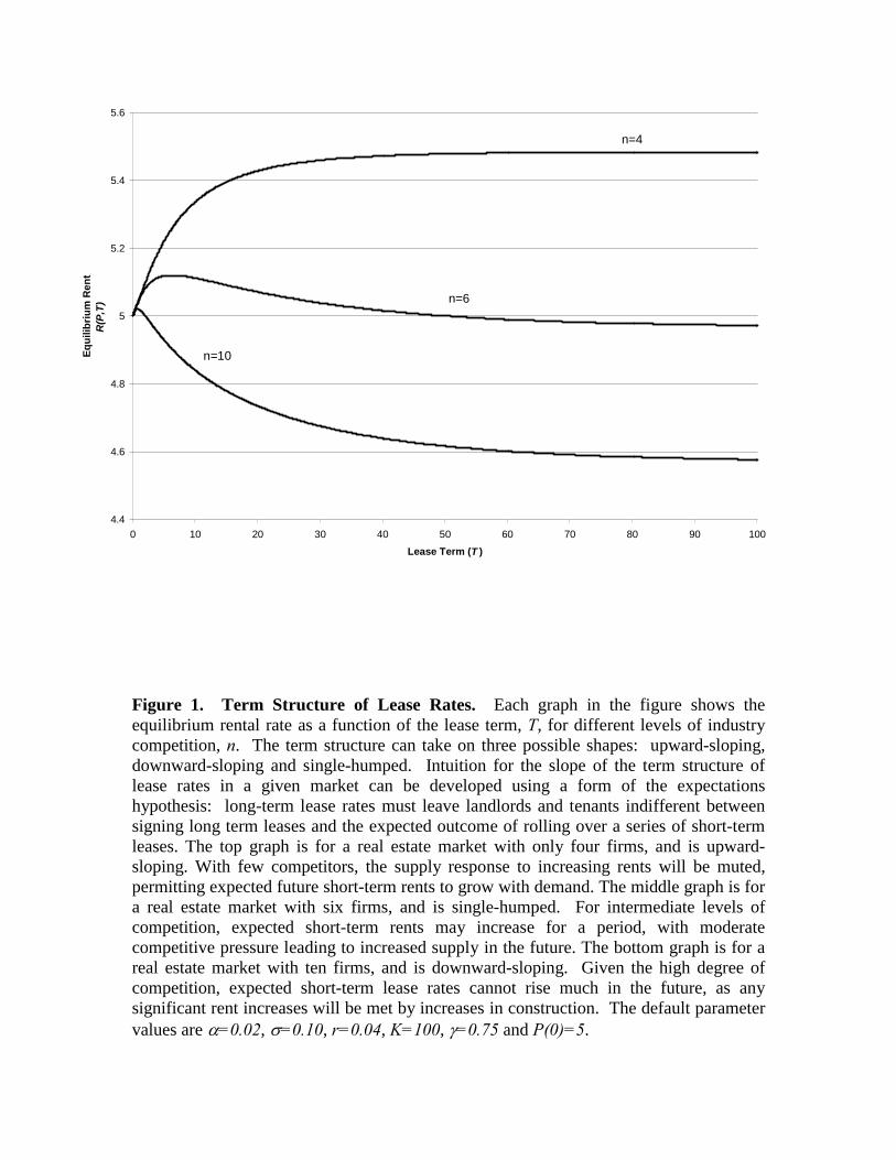
Grenadier (1995) provides a detailed analysis of the term structure of lease rates.Here, I shall con…ne myself to examining the impact of competition on the shape of theterm structure of lease rates. Just as with the Cox, Ingersoll, and Ross or the Vasicekmodels of the term structure of interest rates, the yield curve for rents may take onthree possible shapes: downward-sloping, upward-sloping, and single-humped. Figure1 demonstrates that the degree of competition in a real estate market can determinethe shape of the term structure of rents. Figure 1 displays three term structures, eachwith the same parameters with the exception of the number of …rms competing inthe market. The top curve, which is upward-sloping, corresponds to a market withonly four competitors. The middle curve, which is initially upward-sloping and thendownward-sloping, corresponds to a market with six competitors. The bottom curve,which is downward-sloping, corresponds to a market with ten competitors.
Figure 1 demonstrates a result that holds across a wide range of parameter as-sumptions. For a given instantaneous rent rate P (0), the term structure for marketswith many competitors will be more likely to be downward-sloping, while the termstructure for markets with few competitors will be more likely to be upward-sloping.For markets with intermediate levels of competition, the term structure will be single-humped. The intuition for this result is fairly simple. First, consider an industrywith a large number of competitors. Given the high degree of competition, short-term lease rates cannot rise much in the future, as any signi…cant rent increases willbe met by increases in construction. If the term structure is not downward-sloping,tenants would prefer to roll over a series of short-term leases rather than accept a
15
long-term lease. However, in equilibrium tenants and landlords must be indi¤erentto the form of …nancing of the use of the building. Thus, the term structure ad-justs to allow long-term rents to fall. Second, consider an industry with only a fewcompetitors. With less competition, the supply response to increasing rents will bemuted, permitting future short-term rents to grow with demand. In this case, if theterm structure were not upward-sloping, landlords would prefer rolling over a seriesof short-term leases to accepting a single long-term lease. Once again, to ensureindi¤erence in equilibrium, the term structure adjusts to an upward-sloping shape.Finally, for intermediate levels of competition, short-term rents may increase for aperiod, with moderate competitive pressure leading to increased supply in the future.Thus, short-term rents are expected to increase for a period and then moderate whennew construction ensues. As a result, the term structure takes on an upward slopefor short and intermediate-term leases, and a downward slope for long-term leases.
4 Leases with an Option to Purchase the BuildingA common clause that appears in commercial real estate leases is the option for thetenant to purchase the asset at the end of the lease term. Such clauses are mostcommon in free-standing single tenant buildings. The option to purchase is valued byMcConnell and Schallheim (1983), Grenadier (1996), and Buetow and Albert (1998),all in the context of an exogenous market rent. Here, of course, the lease option isvalued as part of a uni…ed equilibrium.
The option to purchase may be included in a lease to align the incentives of thetenant and landlord. In a lease without a purchase option, the tenant may have littleincentive to maintain the premises beyond the provisions speci…ed in the lease. Sincethe building reverts to the landlord at the end of the lease, the tenant will typicallydeviate from policies that maximize the value of the building. However, when thepurchase option is included in a lease, the tenant has a potential stake in the value ofthe underlying building, and may choose policies that are closer to value maximizing.A similar instance of incentive alignment deals with credit risk. A tenant will be lesswilling to default on a lease with a purchase option, since a purchase option is onlyviable if the tenant pays the contracted rent throughout the lease term.
First, I consider a purchase option with a …xed exercise price. The terms of a leasewith such a purchase option are as follows. Consider a T -year lease, with contractualrental payment ‡ow of Rop, where at the end of the term the tenant may purchasethe building for an exercise price of E .15 I now determine the equilibrium rent onsuch a lease, Rop(P ;T;E).
I begin by valuing the embedded purchase option. The payo¤ on this option is15A common manner of setting the exercise price is to set it at the expected time T building value.
The expected value of a building at T , E fH [P (T )]g, can be written as erT C [P (0); 0; T ], where thefunction C appears in (29).
The …rst boundary condition accounts for P (t) having an absorbing barrier at zero.The second boundary condition represents the option’s payo¤ at expiration. Thethird boundary condition is the Neumann condition that accounts for P (t) having are‡ecting barrier at vn.
where g1, g2, g3, g4, h, ¹ are presented in (30), and q(E) 2 (0; vn) is the unique rootof the expression H[q(E)] ¡ E = 0.16
16 It is simple to demonstrate the properties of q(E). From (22), H(0) ¡ E = ¡E < 0, and byassumption (in order for the option to have value) H(vn ) ¡ E > 0. By continuity, we know at leastone root to H(q)¡ E = 0 exists in the interval (0;vn). Uniqueness is demonstrated by the fact thatH 0 > 0 over this interval.
17
Given the value of the purchase option, I can present the equilibrium lease paymenton a lease with an option to purchase, Rop(P ;T;E). Under such a lease, the tenantreceives the use of the space for T years, plus the value of the option. In return, thelandlord receives the rent ‡ow of Rop(P ;T;E). In equilibrium, these two values mustbe equal:
Figure 2 plots the equilibrium rent on a three-year lease with a purchase optionas a function of the exercise price. First, consider the two extremes of the graph. Ata zero exercise price, the lease becomes equivalent to full ownership of the building,since the lease will always be exercised. Therefore, Rop(P ;T; 0) = r
1¡e¡rT H(P ), asthe present value of the payment ‡ow Rop(P ;T; 0) over T -years must equal the valueof the building. At an exercise price of H(vn) or above, the value of the purchaseoption equals zero, since vn is a re‡ecting barrier and thus P (T) < vn. Thus, the renton a lease with a purchase option with an exercise price in this range must equal therent on a lease without a purchase option: Rop(P ;T;E) = R(P; T ) for E ¸ H (vn).Finally, since the option value is decreasing in the exercise price, @R
op(P ;T;E)@E < 0 for
E < H (vn).I now brie‡y consider another form of lease purchase option clause in which the
exercise price, rather than being a …xed constant, is instead a …xed fraction of theproperty’s market value at the end of the lease term. While this “bargain purchase”structure is rare for traditional …nancial option contracts, it is not uncommon forreal estate purchase option contracts. For example, a lease could specify that at theend of the term the tenant can purchase the property for 95% of its market value(typically determined through a professional appraisal).17 By de…nition, such optionsare always in-the-money. In return, the contracted rent must be higher to re‡ect thevalue of the option granted to the tenant.
In order to value a purchase option with proportional exercise price, consider aT -year lease, with contractual rental payment ‡ow of R̂op, where at the end of theterm the tenant may purchase the building for an exercise price of  ¢H[P (T)], with 2 [0; 1]. The value of this purchase option is simply (1 ¡ Â) ¢ C(P; 0;T), whereC(P; 0;T) is from (29) and represents the value of a call option on the building with
17 In a world with transactions costs, the landlord would prefer selling the property to the tenantfor 95% of the market value if a sale to a third party would entail transactions costs greater than5% (e.g., sales commissions, legal fees, etc.).
18
a zero exercise price. The equilibrium rent on such a lease, R̂op(P ;T; Â), must satisfy:
R̂op(P ;T; Â) = R(P; T) +r
1¡ e¡rT (1¡ Â) ¢ C(P; 0;T ); (39)
="
r1 ¡ exp (¡r ¢ T)
#¢ [H(P )¡ Â ¢ C(P; 0;T ))] ;
where the second equation follows from (31). Note that for  = 0, the value to thetenant is equivalent to ownership of the building, and thus the value of the leasepayments must equal H (P ). In addition, for  = 1 the option has no value and thelease payment is equal to that on a standard T¡year lease.
5 Pre-LeasingIt is not uncommon for space to be pre-leased. This practice is called pre-leasing,and is essentially a forward lease contract. Under pre-leasing, a rent is establishedtoday for a lease term that begins at a speci…c time in the future.
There are several reasons why such pre-leasing contracts exist. First, either theconstruction lender or the take-out lender (the lender who pays o¤ the constructionlender upon completion of construction) may insist upon pre-leasing some portion ofa building prior to lending. This is generally done in order to make sure that thecollateral (the building) is or will be in marketable condition. Second, pre-leasingspace to a quality tenant can be a useful marketing tool for attracting other tenants.This is most common in shopping malls where pre-signing a reputable anchor tenantcan make future leasing to other mall tenants much easier. Third, just as in the caseof traditional forward contracts, tenants who foresee the need to lease space in thefuture may wish to lock in rents and hedge against future market rent increases (justas developers may wish to hedge against future rent decreases).
The equilibrium valuation of pre-leasing contracts is very simple in this setting.Suppose a lease is signed at time zero that permits the tenant to lease space fromtime T1 to T2, where T1 < T2. The lease speci…es a rent ‡ow of RF (P ;T1; T2) to bepaid over this leasing period.
Consider the following two economically equivalent means of purchasing the useof the space over the period [T1; T2]. The …rst is through pre-leasing at the rateRF(P ;T1; T2). The present value of this stream of payments is e¡rT1¡e¡rT2r RF(P ;T1; T2).The second is to form the following portfolio of call options: long one call option onthe building with a zero exercise price and expiration T1 and short one call optionon the building with a zero exercise price and expiration T2. From (29), the value ofthis portfolio equals C(P; 0;T1) ¡C(P; 0;T2): In equilibrium the forward rent ‡ow ofRF(P ;T1; T2) must be such that these alternative means of purchasing the use of thespace are equal:
RF(P ;T1; T2) =r
e¡rT1 ¡ e¡rT2 [C(P; 0;T1)¡ C(P; 0;T2)] : (40)
19
Using the forward rent ‡ow function RF(P ;T1; T2), I can derive the instantaneousforward rate, analogous to the forward interest rate. Let f(P ;T) ´lim
±!0RF (P ;T; T +
±), the forward lease rate over the in…nitesimal period [T; T + ±]. Taking this limityields:
f(P ;T) = ¡erT ¢ @C(P; 0;T)@T
: (41)
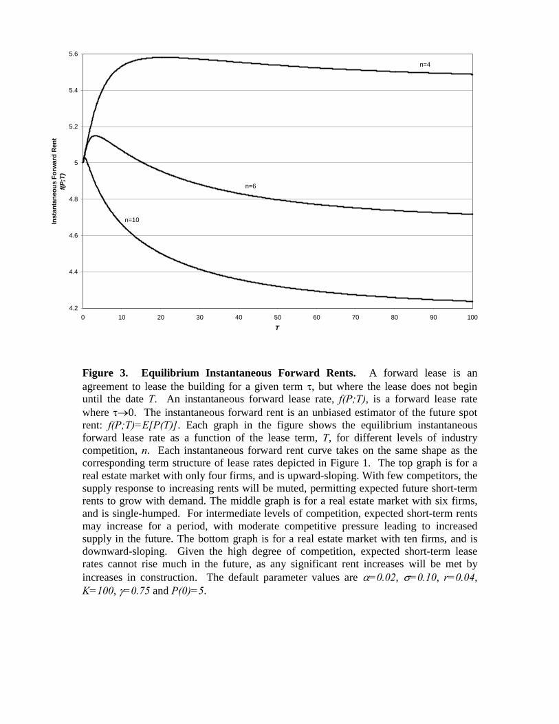
Note that @C(P;0;T )@T = ¡e¡rTE [P (T )].18 Thus, f(P ;T) = E [P (T )], and thus (unlikewith term structure of interest rate models) the forward rent is an unbiased estimatorof the future spot rent.
Figure 3 plots the instantaneous forward rent curve, for three levels of industrycompetition: n = 4; 6; and 10. Several features are worth discussing. First, by de-…nition, f(P ; 0) equals the current spot lease rate P (0), which is 5:0 in this graph.Second, at the other extreme of the forward rent curve, f(P ;1) represents the ex-pected spot rent in the in…nite future. As derived in (19), provided ® > ¾2=2, P (t) hasa long-run stationary distribution with mean ®¡¾2=2
® vn. Thus, the long-run forwardrent converges to a level determined by the degree of industry competitiveness. Third,the forward rent curve may take on three shapes: upward-sloping, downward-slopingand single-humped. For industries with large numbers of competitors, the futurerents are expected to decrease (due to new supply increases outstripping demandgrowth) leading to a downward-sloping forward rent curve. Conversely, for industrieswith small numbers of competitors, the future rents are expected to increase (due todemand growth outstripping supply growth) leading to an upward-sloping forwardrent curve. For industries with intermediate levels of competitors, the forward rentcurve will have a single hump. Notably, the forward rent curve takes on the sameshape as the underlying term structure of lease rates curve. This result is also sharedby the Cox, Ingersoll and Ross model of the term structure of interest rates.
6 Gross Leases and Expense StopsThe leases I have considered thus far are net leases. Under a fully net lease the tenantpays all (or virtually all) of the operating expenses associated with the space. Forexample, a very common leasing arrangement is known as a triple net lease, where thetenant is responsible for maintenance, insurance, and property taxes. In this sectionI consider gross leases, where the landlord is responsible for paying some or all ofthe operating expenses associated with the property. Most leases fall somewhere inbetween the extreme cases of the landlord or the tenant paying all of the operating
18Consider the intuition for this mathematical result. C(P; 0; T) equals the present value of thebuilding’s rent ‡ow from time T onwards. Thus, using the de…nition of a partial derivative, @C
@ Tequals the value of the rent ‡ow from T + " onwards, minus the value of the rent ‡ow from Tonwards, divided by ", where " ! 0. This is simply equal to the negative of the present value of therent ‡ow at time T , or ¡e¡rT E [P (T )].
20
expenses. Such leases, termed hybrid leases, involve both the landlord and tenantpaying a portion of the operating expenses. A particularly interesting case of a hybridlease is a lease with expense stops, where the tenant pays all expenses above a giventhreshold.
It is clear that there is an incentive element to the expense provisions of a lease.When a landlord pays operating expenses, the tenant has little incentive to economizeon usage. When the tenant pays operating expenses, the tenant will internalize suchcosts. It is likely that in leases where the tenant has the most discretion over expenseusage, the net lease form will be the most likely to prevail.
In this section, I begin by considering the general framework for determining theequilibrium gross lease payment. I then move on to two speci…c examples: a fullservice lease and a lease with expense stops.
The general framework for determining the equilibrium gross lease payment issimple. Since the landlord must be indi¤erent between two methods of leasing thespace over a period of time, the present value of the rent ‡ow on a net lease mustequal the present value of the rent ‡ow on a gross lease minus the present value ofthe expenses over the period. Consider a T -year gross lease where the present valueof expenses over the next T -years is denoted by Z(T ). Thus, the equilibrium grosslease payment ‡ow, RG[P; T; Z(T )], can be written as:
1¡ e¡rTr
RG[P; T; Z(T )] =1 ¡ e¡rTr
R(P; T) + Z(T); (42)or;
RG[P; T; Z(T )] = R(P; T ) + r1¡ e¡rT Z(T):
For purposes of the following examples, assume that the ‡ow of expenses, c(t),follows a geometric Brownian motion:
dc = ®ccdt+ ¾ccdzc; (43)
where ®c is the instantaneous conditional expected percentage change in c per unittime, ¾c is the instantaneous conditional standard deviation per unit time, and dzcis the increment of a standard Wiener process.
Consider the example of a full service lease, where all operating expenses are paidfor by the landlord. The present value of expenses, Z(T), is simply:
Z(T) = E"Z T
0e¡rtc(t)dt
#(44)
=c
r ¡ ®ch1 ¡ e¡(r¡®c)T
i;
where c = c(0). Thus, under a full service lease, the equilibrium gross lease paymentis obtained by substituting the expression for Z(T) in (44) into (42).
21
Now, consider the more interesting example of a lease with expense stops. Undera lease with expense stops, the tenant and landlord share expenses by having thetenant pay all expenses above a speci…ed level known as the “stop.” Often, but notalways, the stop is set at the level of actual expenses at the time the lease is signed.Thus, under a lease with expense stops the landlord is protected against in‡ation inexpenses while the tenant has an incentive to keep expenses under control.
Consider a T -year lease with an expense stop at ¹c. The expense reimbursementpayment of the tenant at time t 2 [0; T ] is max[c(t)¡¹c; 0]. This is precisely the payo¤of a call option on c with expiration t and exercise price ¹c. Denote the value of thiscall option by ¨[c; t; ¹c]. Given the log-normality of c(t), this call value is simply theBlack-Scholes value (with proportional dividend parameter r ¡ ®c):
Therefore, the present value of the ‡ow of expense reimbursements is equal to atime-integral of Black-Scholes values:
Z(T) =Z T
0¨[c; t; ¹c]dt: (47)
A solution to this integral, albeit a complicated one, can be written as:
Z(T) = ¹cµ c¹c
¶±1 "µc¹c
¶±2±3N(b1) +
µc¹c
¶¡±2±4N(b2)
#(48)
¡ cr ¡ ®c
e¡(r¡®c)TN(b3) +¹cre¡rTN(b4)
+1c>¹c
(c
r ¡ ®c¡ ¹cr
¡ ¹cµ c¹c
¶±1 "µc¹c
¶±2±3 +
µ c¹c
¶¡±2±4
#);
with:±1 = 1=2¾2c¡®c
¾2c; ±2 =
rr+1=2¾2c±
21
1=2¾2c;
±3 = r¡®c(±1¡±2)2r(r¡®c)±2 ; ±4 = ®c (±1+±2)¡r
2r(r¡®c )±2 ;b1 = ln(c=¹c)
¾cpT
+ ¾c±2pT ; b2 = ln(c=¹c)
¾cpT
¡ ¾c±2pT;
b3 =[ln(c=¹c)+(®c+¾2c=2)T]
¾cpT
b4 = b3 ¡ ¾cpT;
(49)
and 1c>¹c is an indicator function taking the value 1 if c > ¹c, and 0 otherwise.19
Thus, under a lease with expense stops, the equilibrium lease payment is obtained bysubstituting the expression for Z(T) in (48) into (42).
19The solution is continuous and continuously di¤erentiable at c = ¹c.
22
7 Leases with Cancellation OptionsMany leases contain clauses that permit the tenant (and sometimes the landlord)to alter the length of the lease during the term of the lease. A cancellation option(also known as a “kick-out” clause) allows the tenant to terminate the lease priorto expiration. Typically the exercise of the cancellation option results in a pre-determined penalty fee being paid to the landlord. A renewal option allows thetenant to extend the length of the lease at a speci…ed renewal rent, after paying apre-determined renewal fee. Cancellation options and renewal options can be valuedin the same manner. A long-term lease with an option to cancel is economicallyequivalent to a short-term lease with an option to renew. Thus, in this section I focuson leases with cancellation options. An excellent analysis of cancellation and renewaloptions appears in McConnell and Schallheim (1983). This section extends theiranalysis in two ways: embedding the valuation in an industry equilibrium frameworkand by using a continuous-time American option methodology.
Cancellation options are clearly valuable to the tenant, as they permit the tenantto respond to changing market conditions. Suppose a tenant signs a ten-year leasewith a …xed rent of $20 per square foot. The lease contains a cancellation clausethat permits the tenant to cancel the lease at any time after paying a penalty fee.If after three years the prevailing market rent on a seven-year lease is signi…cantlyless than $20 per square foot, the tenant may …nd it optimal to pay the penalty feeand sign a new lease. A cancellation option thus provides insurance against decliningmarket rents, so that if rents fall over the course of the lease term, the tenant hasthe option of signing a new lease at the lower market rent. Some tenants may beparticularly concerned about hedging against being stuck at an above-market rent ifits competitors may be signing new leases in the future and could therefore achieve acost advantage. As in all cases of option valuation, the underlying volatility is a keydeterminant of value. Insuring against rental downturns is likely to be more desirable(and hence more costly) in markets with volatile rents.
Consider the equilibrium valuation of a lease with a cancellation option. The leaseterm is T -years, with a rental payment ‡ow of Rc. The tenant may choose to cancelat any time by paying a penalty fee of F c. Let (P; t;Rc; T; F c) denote the value ofthe payment ‡ow the landlord receives over the period from t to T . must solve thefollowing partial di¤erential equation:
0 = 12¾2P 2PP + ®PP +t ¡ r + Rc; (50)
subject to:
(PL(t); t;Rc; T; F c) =1¡ e¡r(T¡t)
rR(PL(t); T ¡ t) +F c; (51)
P (PL(t); t;Rc; T; F c) =1¡ e¡r(T¡t)
rRP (PL(t); T ¡ t);
23
(P; T ;Rc; T; F c) = 0;P (vn; t;Rc; T; F c) = 0:
The function PL(t) is a trigger function such that whenever P (t) falls to PL(t) thecancellation option is exercised. The …rst boundary condition ensures that when thecancellation option is exercised the landlord receives the current market value of alease from t to T (see Section 3), plus the penalty fee. The second boundary conditionis a smooth-pasting condition that ensures that the trigger function PL(t) is chosenby the tenant so as to minimize . The third boundary condition represents thetermination of the lease at T , and the fourth boundary condition is the Neumanncondition that accounts for the re‡ecting barrier at vn.
In equilibrium, two means of selling the use of the asset for T years must havethe same value. Thus, the equilibrium rent on a lease with a cancellation clause,Rc(P ;T; F c), must solve:
[P; 0;Rc(P ;T; F c); T ; F c] =1 ¡ e¡rTr
R(P; T): (52)
That is, when the lease is signed at time zero, the value of the cash ‡ow to thelandlord under the lease with cancellation option (the left side of the equality) mustequal the value the rental payment ‡ow under a standard T -year lease (the right sideof the equality).
Since the solution to (50) subject to (51) would be numerically quite intensive, Iwill focus on the more tractable problem of an in…nitely-lived lease where T ! 1.Let the value of the payment ‡ow the landlord receives over the in…nite horizon underthe cancelable lease be denoted by 1(P ;Rc;1; F c) = lim
T!1(P; 0;Rc;1; T ; F c), where
Rc;1 is the rent on an in…nitely-lived cancelable lease. For a given rent Rc;1, thesolution can be shown to be:
1(P ;Rc;1; F c) = A1(PL)P¡¯1 +A2(PL)P¯2 +Rc;1
r; (53)
where:
A1(PL) = ¡Rc;1r ¡ F c + v1¡¯2n
¯2(r¡®)P¯2L ¡ PL
r¡®
P¡¯1L + ¯1¯2v¡(¯1+¯2)n P¯2L
; (54)
A2(PL) = ¯1¯2v¡(¯1+¯2)n A1(PL);
PL = arg min0<!<vn
A1(!);
and ¯1 =(®¡ 1
2¾2)+
q(®¡ 1
2¾2)2+2r¾2
¾2 , ¯2 =¡(®¡1
2¾2)+
q(®¡ 1
2¾2)2+2r¾2
¾2 , and where PL isthe exercise trigger value for this in…nite lease.
24
In equilibrium the value of this in…nite stream of lease payments must equalthe value of the underlying building. Thus, the equilibrium lease payment on thein…nitely-lived cancelable lease, Rc;1(P ;F c), must satisfy:
1(P ;Rc;1(P ;F c); F c) = H(P ); (55)
which can easily be solved numerically. At this equilibrium rent, Rc;1(P ;F c), land-lords and tenants are indi¤erent between a lease with a cancellation option and alease without a cancellation option. Note that by substituting the equilibrium rentRc;1(P ;F c) into (54), the equilibrium cancellation option exercise trigger, PL, canbe determined.
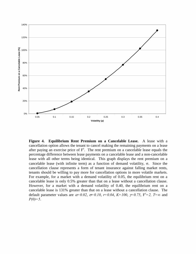
Since the cancellation clause represents a form of tenant insurance against fallingmarket rents, tenants should be willing to pay more for cancellation options in morevolatile markets. Figure 4 con…rms this intuition. Figure 4 plots the percentagerent premium that must be paid on an in…nite-lived cancelable lease for a range ofdemand volatilities. For example, for a market with a demand volatility of 0:05,the equilibrium rent on a cancelable lease is only 0:5% greater than that on a leasewithout a cancellation clause. The value of the insurance feature of the cancellationclause is thus quite low. However, for a market with a demand volatility of 0:40, theequilibrium rent on a cancelable lease is 131% greater than that on a lease without acancellation clause. In volatile markets, the cancellation option is much more likelyto be exercised, and is thus much more costly to purchase.
8 Ground LeasesWhile the basic leasing arrangement in this paper deals with the leasing of a developedbuilding, another leasing arrangement pertains to the leasing of undeveloped land.Under a ground lease, the landowner leases the land to a developer. Upon terminationof a ground lease, the land and all improvements (if any) revert to the landowner.Typically ground leases have long terms (usuallymore than thirty years) with multiplerenewal options. Ground leases also typically dictate the details of the constructionthat can take place on the leased land.
Ground leases introduce a form of ine¢ciency that is di¢cult to deal with inthe context of the present model.20 The Nash equilibrium in the underlying propertymarket is based on the premise of agents maximizing the value of the underlying assets(land values). However, under a ground lease with a …nite term, the developer willunder-build since any building developed during the term will revert to the landlordat the end of the lease. Economically, while a developer that owns the land obtainsan in…nite stream of rent upon construction (e.g., a building), a ground lessee obtains
20Articles that address the incentive compatibility problem regarding the redevelopment options(rather than initial development option) of long-term leases are Capozza and Sick (1991) and Dale-Johnson (2001).
25
a …nite stream of rent upon construction (e.g., the cash ‡ows during the term of the…nite lease).
It is reasonable to wonder why ground leases exist, when it is more e¢cient tosimply sell the land to a developer, assuming the current landowner does not havedevelopment expertise. One explanation is that developers are liquidity constrained,and ground leases may be the most e¢cient means of …nancing the land. A secondexplanation could be tax-based, where the sale might trigger an immediate recognitionof a large gain. A third explanation is simply
However, there are various features of ground leases that mitigate much of theine¢ciency introduced by the …nite term of the ground lease. First, ground leasesare commonly long term and contain multiple extension options, thus approximatingin…nite leases. In addition, ground leases are often signed at or near the point atwhich development begins. Thus, in terms of the value received upon development,the value of a very long term lease will closely approximate the value of the under-lying building. Second, ground leases are frequently renegotiated. Since the overallsurplus is maximized by developing at the equilibrium trigger point, the parties may…nd it mutually bene…cial to make side payments to provide an incentive for optimaldevelopment. Third, ground leases often contain strict provisions concerning devel-opment, including the timing of development.21 All of these factors serve to diminish(although not eliminate) the under-development problem of ground leases.
The simplest ground lease speci…cation, and most consistent with the underlyingequilibrium model, is one of an in…nite term. Under an in…nite ground lease, theground lessor is essentially selling the land in exchange for a ‡ow of lease payments.Recall that the value of the land, L(P ), was derived in (26), where it is assumed thatP < vn, as no development has yet occurred. The ground rent, RG(P ), must be suchthat its perpetuity value equals L(P ), and therefore:
RG(P ) =rKn° ¡ 1
µ Pvn
¶¯: (56)
The di¤erence between a perpetual ground lease and a perpetual lease of a buildingis twofold. First, the ground lessee does not receive the service ‡ow from a buildinguntil the …rst passage time of P (t) to the trigger vn. Second, the ground lesseemust make the cash out‡ow of K upon construction, at the aforementioned …rstpassage time. The di¤erence in the rent between a perpetual lease of a building anda perpetual ground lease is thus:
R(P;1) ¡RG(P ) = r
264P ¡ vn
³Pvn
´¯
r ¡ a +Kµ Pvn
¶¯375 : (57)
21While it would seem that the ground lessor would be indi¤erent to the timing of developmentduring the lease term, in a richer model that included credit risk, the lessor would indeed care.Should the lessee default on the ground rent, the lessor would like to ensure that the land value ismaximized.
26
The …rst term in brackets equals the value of the service ‡ow of the building fromthe initiation of the lease until the …rst passage time of P (t) to the trigger vn. Thesecond term in brackets equals the cost of construction at the …rst passage time ofP (t) to the trigger vn. These two terms are multiplied by r in order to obtain therent ‡ow di¤erence between the two perpetual leases.
9 Escalation ClausesThe basic lease structure in this article calls for a constant rent ‡ow over the entirelease term. Such ‡at rent structures are particularly common on short-term leases.However, on longer-term leases, it is common to …nd rents that vary over the term.Escalation clauses may provide the landlord with a hedge against such factors asunexpected in‡ation or cost ‡uctuations. Escalation clauses in leases specify a rulefor determining the rent level at varying points in time. Examples considered inthis section include rents that move with overall real estate market rents, rents thatmove deterministically, and rents that move with an exogenous index. Clearly, therelationship between leases with …xed rent and leases with variable rents is analogousto the relationship between …xed rate mortgages and adjustable rate mortgages.
Escalation clauses specify an initial rent, various points during the lease wherethe rent is re-set, and the rules by which the rent is re-set. To simplify the modeling,I will assume that the lease is re-set at only one point during the lease. Let the leasebe signed at time zero with a base rent of R0, re-set at time T1, and end at time T2.
9.1 Revaluated RentOne payment structure calls for future lease levels to be marked-to-market. Undersuch a lease (termed a revaluated lease), the rent at speci…ed points in time is re-setto market rent levels. Some leases specify that the rent is re-set only if the marketrent has increases, while others allow the rent to both rise and fall with the market.22
I will consider both speci…cations.First, suppose that the rent is re-set with the market at time T1, whether the
market rent has increased or decreased. This case is obviously very simple. Therent at time T1 will be re-set to R[P (T1); T2 ¡ T1], the equilibrium market rent on a(T2 ¡ T1)-year lease prevailing at time T1. In equilibrium, the initial rent R0 mustequal the market rent on a T1-year lease, R[P; T1]. In the more general case of rentsbeing reset at various points of time throughout the lease, the initial rent will remainequal to the market rent on a lease with term equal to the …rst re-setting point. Inthe limit, as the resetting points occur every instant, the initial lease rate will simplyequal the instantaneous rate P (0).
22For a detailed treatment of the former speci…cation, sometimes known as upward-only adjustingleases, see Ambrose, Hendershott and Klosek (2001).
27
Second, suppose that the rent is re-set to the market rent at time T1 if rents haveincreased, but kept constant otherwise. Thus, the rent will be re-set at time T1 toequal max fR[P (T1); T2 ¡ T1]; R0g. The value of the rental payments under such alease can be expressed in terms of various leasing structures previously analyzed inthis article, notably cancellation options and pre-leasing contracts. Since
the value of the payment stream on this lease over the period [T1; T2] equals thevalue of the three right-hand side cash ‡ows. The value of the constant payment‡ow of R0 is simply R0
r (e¡rT1 ¡ e¡rT2 ). The value of the market rental stream of
R[P (T1); T2 ¡ T1] must equal the value of the pre-leasing rent of RF (P ;T1; T2), ore¡rT1¡e¡rT2
r RF(P ;T1; T2), since these are two equivalent ways of leasing space overthis period. The value of the rental stream of minfR[P (T1); T2 ¡ T1]; R0g is equal tothe value of a lease cancellation option (of the European variety), with initial rentR0 and with a zero penalty fee. Denote the value of this particular lease cancellationoption by ¤(P;R0; T1; T2).
LetM (P; T1; T2; R0) equal the value of the cash ‡ows under this revaluation lease.This must equal the value of the constant payment ‡ow of R0 over the …rst T1 years,plus the sum of the three values in the previous paragraph. Simplifying, this yields:
M(P; T1; T2; R0) =R0
r (1¡ e¡rT2) + e¡rT1 ¡ e¡rT2
r RF (P ;T1;T2) ¡ ¤(P;R0; T1; T2):(59)
In equilibrium, the equilibrium initial rent value, R¤0, must be set so that the valueof the rent ‡ows equals that on a standard T2-year lease:
M (P; T1; T2; R¤0) =R(P; T2)r
(1¡ e¡rT2 ): (60)
9.2 Graduated RentA second payment structure calls for simple, pre-determined rent increases. Undersuch a lease (termed a graduated lease), the lease speci…es non-stochastic rent changes(step-ups) at various points in time. Valuing such leases is a trivial matter.
Consider the example of a lease with initial rent R0, stepped up at T1 by thegrowth rate of g, and ending at T2. Thus, the stepped-up rent at T1 is egT1R0. Thepresent value of these lease payments is:
R0
r
h1¡ e¡rT1 + egT1(e¡rT1 ¡ e¡rT2)
i: (61)
In equilibrium, the equilibrium initial rent value, R¤0, must be set so that the valueof the rent ‡ows equals that on a standard T2-year lease:
R¤0r
h1¡ e¡rT1 + egT1(e¡rT1 ¡ e¡rT2)
i=R(P; T2)r
(1 ¡ e¡rT2) (62)
28
or;
R¤0 =R(P; T2)(1¡ e¡rT2 )
[1¡ e¡rT1 + egT1 (e¡rT1 ¡ e¡rT2)]:
9.3 Indexed RentA third payment structure calls for the rent to move with an exogenous, publiclyobservable index. Common indices include the CPI and PPI. The rent may increaseone-for-one with the index, or move with a fraction of the index.
Consider the example of a lease that is adjusted to ½% of the growth of the indexI(t), where the index follows the geometric Brownian motion:
dI = ®IIdt+ ¾IIdzI : (63)
Speci…cally, let the initial rent equal R0, and let the rent be changed to ½ ¢ I(T1)I(0) R0 atT1. The present value of these lease payments is:
R0
"1 ¡ e¡rT1r
+ ½ ¢ e¡(r¡®I)T1 ¡ e¡(r¡®I)T2
r ¡ ®I
#: (64)
In equilibrium, the equilibrium initial rent value, R¤0, must be set so that the valueof the rent ‡ows equals that on a standard T2-year lease:
R¤0
"1 ¡ e¡rT1r
+ ½ ¢ e¡(r¡®I)T1 ¡ e¡(r¡®I)T2
r ¡ ®I
#=R(P; T2)r
(1¡ e¡rT2) (65)
or;
R¤0 =R(P; T2)(1¡ e¡rT2 )·
1¡ e¡rT1 + ½r ¢ e¡(r¡®I)T1¡e¡(r¡®I )T2r¡®I
¸:
10 Leases with ConcessionsIt is not unusual for leases to contain one or more inducements to attract tenants.Such inducements are known as concessions and are most common during real estatemarket downturns. Lease concessions may include allowing free rent periods, payingmoving costs and providing above-normal tenant improvement allowances. A freerent provision allows the tenant to use the space for an initial period without payingrent. The free rent period can be anywhere from one month to over a year on along-term lease. Tenant improvement allowances are cash allowances provided by thelandlord to pay for the costs of interior improvements in the leased space. While somebase level of tenant improvement allowances is typically granted in a lease, anythingbeyond this base level is considered a concession.
In any rational equilibrium, it is clear that leases o¤ering concessions will resultin higher rental rates. Empirically, this contributes to the well-observed phenomenon
29
of “sticky” quoted rents. Quoted rents are much less volatile than e¤ective rentsthat take into account the impact of concessions during the lease term. There areseveral potential reasons why leases provide concessions in return for higher rents.The …rst explanation is that tenants are more likely to be liquidity constrained thanlandlords. Thus, concessions are a means of providing …nancing to tenants, especiallyduring a period of high moving and start-up costs. A second explanation is that usingconcessions may assist landlords in negotiating with multiple tenants. While quotedrents are reported to the public, concessions are typically more private and the resultof negotiations between landlords and tenants. Landlords may …nd that keepingtheir reservation rent private may improve their multilateral bargaining position withcurrent and future tenants. A third explanation could be that there exists somefriction or regulatory feature that makes it in the landlord’s interest to report highrecurring rentals (even at the expense of concessions granted). For example, a landlordmay be able to achieve better re…nancing terms if appraisals do not fully take intoaccount concessions, but instead use some multiple of rents for valuation purposes.
Finding the equilibrium rent on a lease with concessions is quite simple in thecurrent context. Consider two types of concessions: lump sum concessions such asmoving allowances and free rental periods. Let ¹C denote the dollar value of the lumpsum concessions, and ¿ the period of the T -year lease under which no rent is paid(where ¿ < T). The rent paid on this lease is denoted by Rcon(P; T ; ¹C; ¿ ).
In equilibrium, the landlord must be indi¤erent between a lease with concessionsand a lease without concessions. In a lease with concessions, the landlord receivesthe rent ‡ow of Rcon(P; T ; ¹C; ¿ ) from ¿ to T , minus the lump sum cost ¹C. Under alease without concessions, the landlord receives a lease ‡ow of R(P; T) from 0 to T .Equating these two lease values and solving for Rcon(P; T ; ¹C; ¿ ) results in:
Rcon(P; T ; ¹C; ¿) =1¡ e¡rTe¡r¿ ¡ e¡rTR(P; T) +
re¡r¿ ¡ e¡rT
¹C: (66)
As an illustration, suppose that for various reasons the landlord would like to re-port a quoted rent that is the highest possible rent on a lease without concessions. Themaximum rent would be achieved if the instantaneous rent equals its upper re‡ectingbarrier,R(vn; T ). Suppose, however, the current instantaneous rent is less than its up-per bound, P < vn. Thus, in order to set a quoted rent of Rcon(P; T ; ¹C; ¿) = R(vn; T ),the package of concessions ( ¹C; ¿) would have to solve:
R(vn; T) =1¡ e¡rTe¡r¿ ¡ e¡rTR(P; T) +
re¡r¿ ¡ e¡rT
¹C: (67)
Obviously there are an in…nite number of combinations of ¹C and ¿ that can solvethis equality. However, …rst suppose this is accomplished solely through a free rentperiod. Then, ¹C = 0 and ¿ must equal:
¿ = ln
24
Ãe¡rT +
³1 ¡ e¡rT
´ R(P; T)R(vn; T )
!¡r35 : (68)
30
Note that @¿@P < 0, and thus the greater the distance of the current rent P from itsmaximum vn, the greater the free rent period. Consider the two extremes. If thecurrent rent is at its maximum (P = vn), then no free rent is necessary and ¿ = 0.If the current rent is at is minimum (P = 0), then the free rent period must be theentire lease term (¿ = T).
Conversely, suppose equality (67) is accomplished solely through lump-sum con-cessions. Then, ¿ = 0 and ¹C must equal:
¹C =1 ¡ e¡rTr
[R(vn;T )¡R(P; T)] : (69)
Note that @ ¹C@P < 0, and thus the greater the distance of the current rent P fromits maximum vn, the greater the required lump-sum concession. Consider the twoextremes. If the current rent is at its maximum (P = vn), then no concessions arenecessary and ¹C = 0. If the current rent is at is minimum (P = 0), then the requiredlump-sum concession is 1¡e¡rT
r R(vn; T ).
11 Sale-Leaseback TransactionsUnder a sale-leaseback agreement, the owner of a building (usually the sole occupant)sells the building and simultaneously signs a lease on the building. Such transactionsare typically justi…ed as a form of …nancing; the seller/tenant uses the sales proceedsfor business expansion and the lease payments represent …nancing payments. Thisjusti…cation makes most sense for small …rms that have di¢culty obtaining …nancing,however it may be less compelling for the many large corporations that engage insale-leasebacks of their corporate headquarters.
Clearly, modeling the sale-leaseback transaction is quite simple. There are twocomponents of the transaction: setting the sales price and setting the lease terms.If the sales price equals the true market value of the building, then the lease ratemust equal the equilibrium lease rate on a standard lease. However, if the sales pricedi¤ers from the market value of the asset, then the lease terms will also di¤er fromthe equilibrium lease rate on a standard lease.
Consider the following sale-leaseback arrangement. The building is sold for S ,and simultaneously leased back for T -years at a rental rate of Y . The market value ofthe building is H(P ), and the equilibrium rent on a standard T -year lease is R(P; T ).In equilibrium, the di¤erence between the market value of the building and the salesprice must equal the di¤erence between the market value of the equilibrium leasepayments and the agreed upon lease payments:
H(P ) ¡ S =1¡ e¡rTr
[R(P; T)¡ Y ] : (70)
Therefore, for a given sales price, S, the equilibrium sale-leaseback rental rate, Y (P; S; T),
31
equals:Y (P; S; T) = R(P; T) + r
1¡ e¡rT [S ¡H(P )] : (71)
There are two degrees of freedom in setting the contract terms: S and Y . Considera few examples of possible contract terms. First, suppose that the seller would like torecord a sales price that represents the maximum obtainable from a direct sale,H (vn).Then, using (71), the equilibrium lease rate must beR(P; T)+ r
1¡e¡rT [H(vn) ¡H(P )].Second, suppose the seller wishes to sell the property at the same price at which theproperty was purchased, where the purchase price was H(P̂ ) and where P̂ was themarket rent prevailing at the time of purchase. Then, using (71), the equilibriumlease rate must be R(P; T ) + r
1¡e¡rThH(P̂ )¡H(P )
i. Finally, consider the case in
which seller is willing to pay the maximum standard rent of R(vn; T ) in order toachieve a high selling price. Then, the equilibrium sales price must be H(P ) +1¡e¡rTr [R(vn; T )¡R(P; T)].
12 ConclusionI derive a model that provides a uni…ed equilibrium approach to valuing real es-tate lease contracts. The underlying real estate asset market equilibrium is modeledas a continuous-time Nash equilibrium in which …rms choose optimal developmentstrategies in the face of evolving demand uncertainty. Using an option pricing ap-proach, the real estate leasing market is then modeled as a contingent claim on theequilibrium building value. Given the underlying structure of the real estate mar-ket (number of developers, the demand curve for space and the properties of thestochastic process underlying demand), endogenous processes for rent, constructionstarts, building values and land values are derived. This equilibrium framework is‡exible enough to value a wide variety of realistic leasing contracts. Examples of leas-ing contracts valued in this article are purchase options, pre-leasing, net and grossleases, cancellation options, ground leases, escalation clauses, lease concessions andsale-leaseback contracts.
Several extensions of the model would prove interesting. First, the model couldbe empirically tested using actual lease contracts. The availability of large and reli-able samples of individual lease contracts is currently di¢cult to obtain. The modelsuggests that equilibrium lease rates will be sensitive to the degree of competition inthe local real estate market, the shape of the demand curve for space, the parametersunderlying the shock term for demand, and the speci…c terms of the contract (e.g.,maturity, embedded options, operating expense provisions, etc.). Second, the under-lying assumption of identical …rms could be weakened. It is likely to be the case thatin any given real estate markets developers di¤er in their skill levels, experience, and…nancial strength. While providing greater realism to the model, the concomitantloss of the simplifying feature of a symmetric equilibrium would greatly diminish thetractability of the model.
32
References[1] Ambrose, B., P. Hendershott and M. Klosek, 2001, “Pricing Upward-Only Ad-
justing Leases,” Journal of Real Estate Finance and Economics, Forthcoming.
[2] Baldursson, F., 1997, “Irreversible Investment Under Uncertainty in Oligopoly,”Journal of Economic Dynamics and Control 22, 627-644.
[3] Brealey, R., and C. Young, 1980, “Debt, taxes and leasing: A note,” Journal ofFinance 35, 1245-1250
[4] Brennan, M.J., and A. Kraus, 1982, “The equilibrium term structure of leaserates,” Working paper no. 862 (The University of British Columbia, Vancouver,British Columbia).
[5] Brennan, M.J., and E. Schwartz, 1985, “Evaluating Natural Resource Invest-ments,” Journal of Business 58, 135-157.
[6] Buetow, G., and J. Albert, 1998, “The Pricing of Embedded Options in RealEstate Contracts,” Journal of Real Estate Research 15, 253-265.
[7] Bulan, L., “Real Options, Irreversible Investment and Firm Uncertainty: NewEvidence from U.S. Firms,” Working paper, Columbia School of Business.
[8] Bulan, L., C. Mayer and C.T. Somerville, 2001, “Real Options, Competition andInvestment: Evidence from Real Estate Development,” Working paper, Whar-ton.
[9] Capozza, D., and G. Sick, 1991, “Valuing Long Term Leases: The Option toRedevelop,” Journal of Real Estate Finance and Economics 4, 209-223.
[10] Constantinides, G.M., 1984, “Warrant Exercise and Bond Conversion in Com-petitive Markets,” Journal of Financial Economics 13, 371-397.
[11] Cox, J.C., J.E. Ingersoll, Jr., and S.A. Ross, 1985, “A theory of the term struc-ture of interest rates,” Econometrica 53, 385-408.
[12] Dale-Johnson, D., 2001, “Long-Term Ground Leases, the Redevelopment Optionand Contract Incentives,” Real Estate Economics 29, 451-484.
[13] Dixit, A., 1989, “Entry and Exit Decisions Under Uncertainty,” Journal of Po-litical Economy 97, 620-638.
[14] Dixit, A. K., and R. S. Pindyck, 1994, “Investment Under Uncertainty,” Prince-ton University Press, Princeton, New Jersey.
33
[15] Farnsworth, H., and R. Bass, 1998, “The Term Structure with Semi-CredibleTargeting,” Working paper, Washington University.
[16] Grenadier, S.R., 1995, “Valuing Lease Contracts: A Real-Options Approach,”Journal of Financial Economics 38, 297-331.
[17] Grenadier, S.R., 1996, “The Strategic Exercise of Options: Development Cas-cades and Overbuilding in Real Estate Markets,” Journal of Finance 51, 1653-1679.
[18] Grenadier, S.R., 1999, “Information Revelation Through Option Exercise,” Re-view of Financial Studies 12, 95-130.
[19] Grenadier, S.R., 2000, “Game Choices: The Intersection of Real Options andGame Theory,” Risk Books, London.
[20] Grenadier, S.R., 2002, “Option Exercise Games: An Application to the Equilib-rium Investment Strategies of Firms,” Review of Financial Studies 15, 691-721.
[21] Harrison, J. M., 1985, “Brownian Motion and Stochastic Flow Systems,” Wiley,New York.
[22] Kulatilaka, N., and E. Perotti, 1998, “Strategic Growth Options,” ManagementScience 44, 1021-1031.
[23] Lambrecht, B., and W. Perraudin, 1999, “Real Options and Preemption UnderIncomplete Information,” Working paper, University of Cambridge.
[24] Leahy, J.V., 1993, “Investment in Competitive Equilibrium: The Optimality ofMyopic Behavior,” Quarterly Journal of Economics 108, 1105-1133.
[25] Lewis, C.M., and J.S. Schallheim, 1992, Are debt and leases substitutes?, Journalof Financial and Quantitative Analysis 27, 497-511.
[26] Majd, S., and R. Pindyck, 1987, “Time to Build, Option Value, and InvestmentDecisions,” Journal of Financial Economics 18, 7-28.
[27] McConnell, J.J., and J.S. Schallheim, 1983, “Valuation of asset leasing con-tracts,” Journal of Financial Economics 12, 237-261.
[28] McDonald, R., and D. Siegel, 1986, “The Value of Waiting to Invest,” QuarterlyJournal of Economics 101, 707-727.
34
[29] Miller, M.H., and C.W. Upton, 1976, “Leasing, buying, and the cost of capitalservices,” Journal of Finance 31, 761-786.
[30] Miles, M., and N. Tolleson, 1997, “A Revised Look at How Real Estate Compareswith Other Major Components of Domestic Investment Universe,” Real EstateFinance 14, 11-20.
[31] Myers, S.C., D. Dill, and A. Bautista, 1976, “Valuation of …nancial lease con-tracts,” Journal of Finance 31, 799-819.
[32] Schall, L.D., 1974, “The lease-or-buy and asset acquisition decision,” Journal ofFinance 29, 1203-1214.
[33] Smets, F.R., 1993, “Essays on Foreign Direct Investment,” Unpublished disser-tation, Yale University.
[34] Smith, C.W., Jr., 1979, “Applications of option pricing analysis,” in: J.L. Bick-sler, ed., Handbook of Financial Economics (North-Holland, Amsterdam).
[35] Smith, C.W., Jr., and L.M. Wakeman, 1985, “Determinants of corporate leasingpolicy,” Journal of Finance 40, 895-908.
[36] Spatt, C.S., and F.P. Sterbenz, 1988, “Warrant Exercise, Dividends, and Rein-vestment Policy,” Journal of Finance 43, 493-506.
[37] Titman, S., 1985, “Urban Land Prices Under Uncertainty,” American EconomicReview 75, 505-514.
[38] Triantis, A., and J. Hodder, 1990, “Valuing Flexibility as a Complex Option,”Journal of Finance 45, 549-565.
[39] Vasicek, O., 1977, “An Equilibrium Characterization of the Term Structure,”Journal of Financial Economics 5, 177-188.
[40] Williams, J. T., 1993, “Equilibrium and Options on Real Assets,” Review ofFinancial Studies 6, 825-850.
35
Figure 1. Term Structure of Lease Rates. Each graph in the figure shows the equilibrium rental rate as a function of the lease term, T, for different levels of industry competition, n. The term structure can take on three possible shapes: upward-sloping, downward-sloping and single-humped. Intuition for the slope of the term structure of lease rates in a given market can be developed using a form of the expectations hypothesis: long-term lease rates must leave landlords and tenants indifferent between signing long term leases and the expected outcome of rolling over a series of short-term leases. The top graph is for a real estate market with only four firms, and is upward-sloping. With few competitors, the supply response to increasing rents will be muted, permitting expected future short-term rents to grow with demand. The middle graph is for a real estate market with six firms, and is single-humped. For intermediate levels of competition, expected short-term rents may increase for a period, with moderate competitive pressure leading to increased supply in the future. The bottom graph is for a real estate market with ten firms, and is downward-sloping. Given the high degree of competition, expected short-term lease rates cannot rise much in the future, as any significant rent increases will be met by increases in construction. The default parameter values are �=0.02, �=0.10, r=0.04, K=100, �=0.75 and P(0)=5.
4.4
4.6
4.8
5
5.2
5.4
5.6
0 10 20 30 40 50 60 70 80 90 100Lease Term (T )
Equi
libriu
m R
ent
R(P
,T)
n=4
n=10
n=6
Figure 2. Equilibrium Rent on a Lease With an Option to Purchase. This graph shows the equilibrium rent on a lease with the option to purchase the building as a function of the option exercise price, E. A lease with a purchase option provides the tenant with a European call option on the building with an exercise price of E and an expiration date equal to the term of the lease. Consider the equilibrium rent at two extremes of the range of E. At an exercise price of zero, the lease becomes economically equivalent to outright ownership of the building. At any exercise price greater than or equal to H(vn), the option will never be exercised, as H(vn) represents an upper reflecting barrier on the building’s value. In this figure, H(vn)=128.57. Thus, for leases with E> H(vn), the rent must be the same as that on leases without purchase options. For all 0<E< H(vn), the equilibrium rent is decreasing in E. The default parameter values are �=0.02, �=0.10, r=0.04, K=100, �=0.75, T=3 and P(0)=5.
Figure 3. Equilibrium Instantaneous Forward Rents. A forward lease is an agreement to lease the building for a given term �, but where the lease does not begin until the date T. An instantaneous forward lease rate, f(P;T), is a forward lease rate where ��0. The instantaneous forward rent is an unbiased estimator of the future spot rent: f(P;T)=E[P(T)]. Each graph in the figure shows the equilibrium instantaneous forward lease rate as a function of the lease term, T, for different levels of industry competition, n. Each instantaneous forward rent curve takes on the same shape as the corresponding term structure of lease rates depicted in Figure 1. The top graph is for a real estate market with only four firms, and is upward-sloping. With few competitors, the supply response to increasing rents will be muted, permitting expected future short-term rents to grow with demand. The middle graph is for a real estate market with six firms, and is single-humped. For intermediate levels of competition, expected short-term rents may increase for a period, with moderate competitive pressure leading to increased supply in the future. The bottom graph is for a real estate market with ten firms, and is downward-sloping. Given the high degree of competition, expected short-term lease rates cannot rise much in the future, as any significant rent increases will be met by increases in construction. The default parameter values are �=0.02, �=0.10, r=0.04, K=100, �=0.75 and P(0)=5.
4.2
4.4
4.6
4.8
5
5.2
5.4
5.6
0 10 20 30 40 50 60 70 80 90 100T
Inst
anta
neou
s Fo
rwar
d R
ent
f(P;T
)
n=10
n=6
n=4
Figure 4. Equilibrium Rent Premium on a Cancelable Lease. A lease with a cancellation option allows the tenant to cancel making the remaining payments on a lease after paying an exercise price of Fc. The rent premium on a cancelable lease equals the percentage difference between lease payments on a cancelable lease and a non-cancelable lease with all other terms being identical. This graph displays the rent premium on a cancelable lease (with infinite term) as a function of demand volatility, �. Since the cancellation clause represents a form of tenant insurance against falling market rents, tenants should be willing to pay more for cancellation options in more volatile markets. For example, for a market with a demand volatility of 0.05, the equilibrium rent on a cancelable lease is only 0.5% greater than that on a lease without a cancellation clause. However, for a market with a demand volatility of 0.40, the equilibrium rent on a cancelable lease is 131% greater than that on a lease without a cancellation clause. The default parameter values are �=0.02, �=0.10, r=0.04, K=100, �=0.75, Fc=2, T=∞ and P(0)=5.