Osaka City University Japan AN EQUIVALENCE THEOREM FOR LEFSCHETZ FIBRATIONS OVER THE DISK Daniele Zuddas Korea Institute for Advanced Study Republic of Korea Joint with Nikos Apostolakis Riccardo Piergallini CUNY University of Camerino http://newton.kias.re.kr/ ~ zuddas [email protected]
Transcript
Osaka City University
Japan
AN EQUIVALENCE THEOREM FOR LEFSCHETZ
FIBRATIONS OVER THE DISK
Daniele Zuddas
Korea Institute for Advanced StudyRepublic of Korea
Joint with
Nikos Apostolakis Riccardo PiergalliniCUNY University of Camerino
A LF can be thought as a complex-valued Morse function f(z, w) = z2 + w2. Hence,f : V ⌃ B2 determines a handlebody decomposition of V , with only handles of index ⇥ 2(a 2-handlebody).
γ−1i
γi+1
1−1γi+1 −1
From Lefschetz fibrations to Kirby diagrams.
Hurwitz moves change the 2-handlebody structure up to standard Kirby moves (we call2-equivalence this equivalence relation induced on 2-handlebodies).
3Let the Dehn twist ⌅i be about the curve ci. If all the ci’s are non-zero in H1(F ), we
say that f is allowable.
Two monodromy sequences determine equivalent Lefschetz fibrations i� they can berelated by Hurwitz moves and cyclic permutations:
A LF can be thought as a complex-valued Morse function f(z, w) = z2 + w2. Hence,f : V ⌃ B2 determines a handlebody decomposition of V , with only handles of index ⇥ 2(a 2-handlebody).
γ−1i
γi+1
1−1γi+1 −1
From Lefschetz fibrations to Kirby diagrams.
Hurwitz moves change the 2-handlebody structure up to standard Kirby moves (we call2-equivalence this equivalence relation induced on 2-handlebodies).
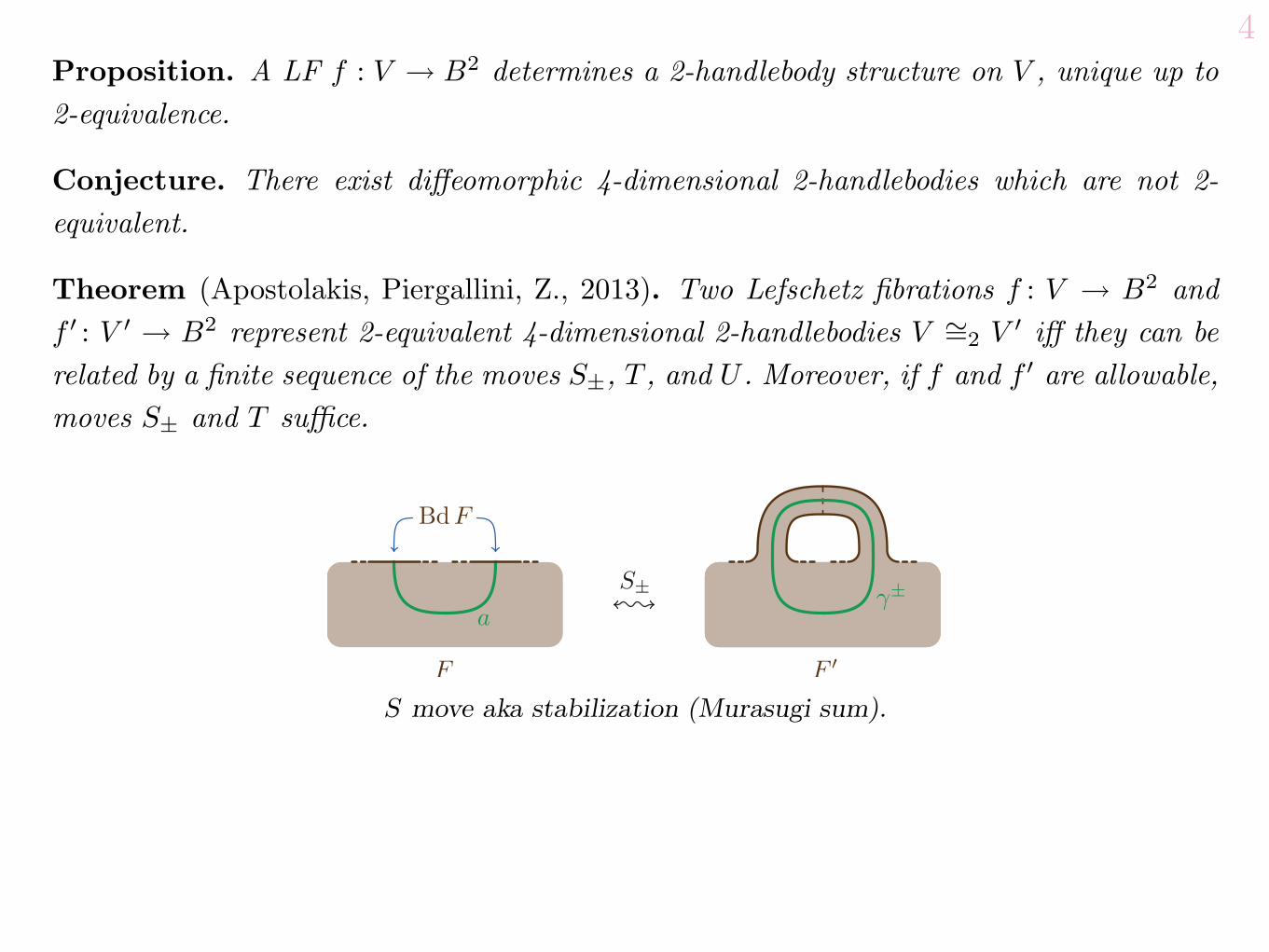
4Proposition. A LF f : V ⌃ B2 determines a 2-handlebody structure on V , unique up to2-equivalence.
Conjecture. There exist di�eomorphic 4-dimensional 2-handlebodies which are not 2-equivalent.
Theorem (Apostolakis, Piergallini, Z., 2013). Two Lefschetz fibrations f : V ⌃ B2 andf ⇥ : V ⇥ ⌃ B2 represent 2-equivalent 4-dimensional 2-handlebodies V ⌅=2 V ⇥ i� they can berelated by a finite sequence of the moves S±, T , and U . Moreover, if f and f ⇥ are allowable,moves S± and T su⇥ce.
S move aka stabilization (Murasugi sum).
5
+
−
+
T move.
0
0
Proof of the T move.
5
+
−
+
T move.
0
0
Proof of the T move.
5
+
−
+
T move.
0
0
Proof of the T move.
6
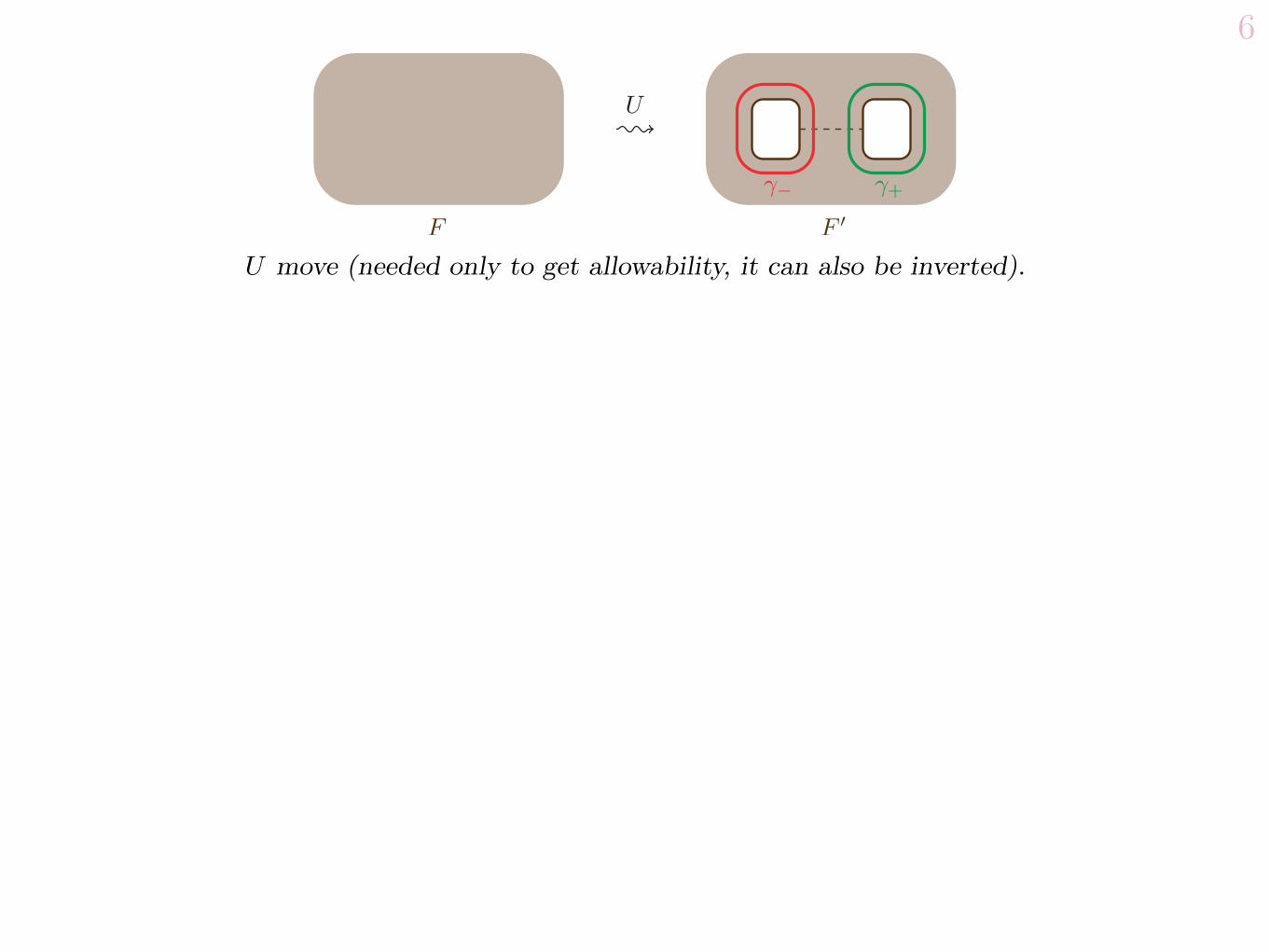
U move (needed only to get allowability, it can also be inverted).
2 Open books on 3-manifolds
Let M be a 3-manifold, L ⇧M a fibered link.
M � L⌃ S1.
First, we see how Lefschetz fibrations are related with open books. This is very simple.Given a Lefschetz fibration with bounded fiber f : V ⌃ B2, just take the restriction�f = f|⇤V : �V ⌃ B2 and this is an open book decomposition of the 3-manifold M = �V
(actually, restrict to M � f�1(0)⌃ B2 � 0⌃ S1).
The restriction to the boundary of the moves S, T , and U , which we denote respectivelyby �S, �T , and �U , preserve the oriented 3-manifold up to di�eomorphisms.
6
U move (needed only to get allowability, it can also be inverted).
2 Open books on 3-manifolds
Let M be a 3-manifold, L ⇧M a fibered link.
M � L⌃ S1.
First, we see how Lefschetz fibrations are related with open books. This is very simple.Given a Lefschetz fibration with bounded fiber f : V ⌃ B2, just take the restriction�f = f|⇤V : �V ⌃ B2 and this is an open book decomposition of the 3-manifold M = �V
(actually, restrict to M � f�1(0)⌃ B2 � 0⌃ S1).
The restriction to the boundary of the moves S, T , and U , which we denote respectivelyby �S, �T , and �U , preserve the oriented 3-manifold up to di�eomorphisms.
7Theorem (Apostolakis, Piergallini, Z. (2013)). Two Lefschetz fibrations f : V ⌃ B2 andf ⇥ : V ⇥ ⌃ B2 have di�eomorphic boundaries if and only if f and f ⇥ can be related by themoves S±, T , U , P , Q, and fibered equivalence. Actually, U is not really needed if f andf ⇥ are allowable.
The move P .
The move Q.
P correspond to connected sum with CP2. Q is the addition of a pair of oppositeconsecutives Dehn twists in the monodromy sequence, along parallel curves. It correspondsto trading a 1-handle for a 2-handle.
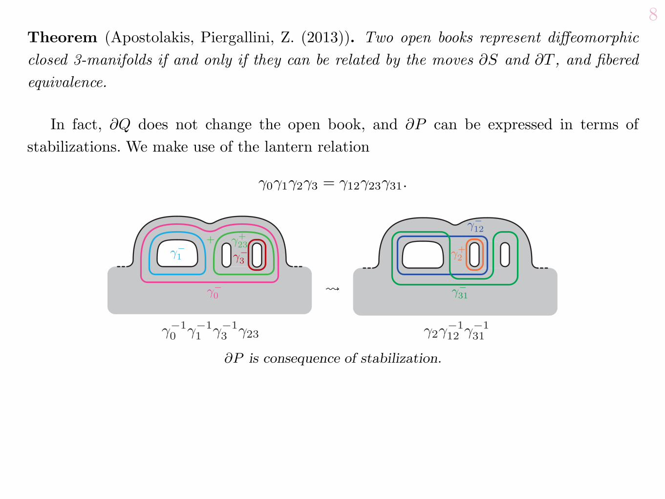
8Theorem (Apostolakis, Piergallini, Z. (2013)). Two open books represent di�eomorphicclosed 3-manifolds if and only if they can be related by the moves �S and �T , and fiberedequivalence.
In fact, �Q does not change the open book, and �P can be expressed in terms ofstabilizations. We make use of the lantern relation
⌅0⌅1⌅2⌅3 = ⌅12⌅23⌅31.
γ−10 γ−1
1 γ−13 γ23 γ2γ
−112 γ−1
31
γ−0
γ−1 γ−
3
γ+23
γ+2
γ−12
γ−31
�P is consequence of stabilization.
This should be compared with a theorem of Harer, who first obtained the moves foropen book decompositions.
Theorem (Harer, 1982). Two open books on the same 3-manifold can be related by stabil-izations, double twistings, and fibered isotopy.
9
c1
c2
A
F1 F2
Harer’s double twisting.
We have already discussed stabilizations. So, we just explain double twisting quickly.Pick two simple curves c1 ⇧ F1 and c2 ⇧ F2 contained in two di�erent pages F1 and F2 ofan open book. Suppose that there is an annulus A ⇧ M with �A = c1� c2. Let c⇥
i ⇧ Fi andc⇥⇥i ⇧ A be the framings induced respectively by Fi and A on ci. If c⇥⇥
i + (�1)i = c⇥i � ⌥i for
some ⌥i = ±1 then the open book with monodromy ⌅f ⇤ t⇥1c1⇤ t⇥2
c2still represents M because
the two new Dehn twists give two opposite ±1-surgeries along isotopic knots (we denoteby tc the right-handed Dehn twist along the curve c ⇧ F ).
The annulus is not related to the open book, apart the constraints on the framings,and can intersect the open book in a rather arbitrary way. So, this move can be quitedestructive for the original open book.
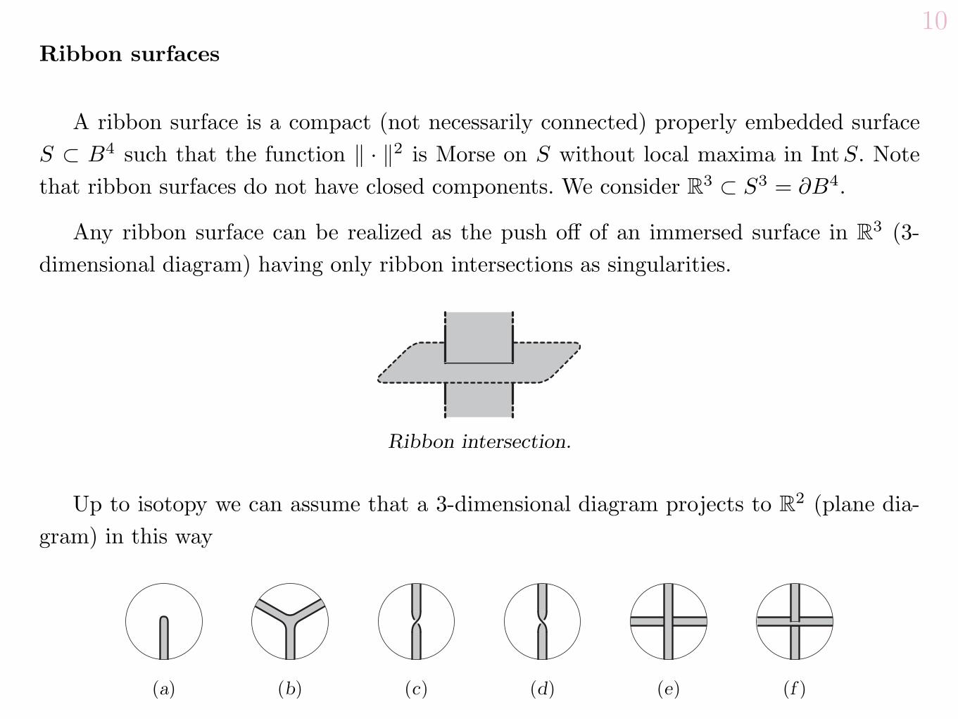
10Ribbon surfaces
A ribbon surface is a compact (not necessarily connected) properly embedded surfaceS ⇧ B4 such that the function · 2 is Morse on S without local maxima in IntS. Notethat ribbon surfaces do not have closed components. We consider R3 ⇧ S3 = �B4.
Any ribbon surface can be realized as the push o� of an immersed surface in R3 (3-dimensional diagram) having only ribbon intersections as singularities.
Ribbon intersection.
Up to isotopy we can assume that a 3-dimensional diagram projects to R2 (plane dia-gram) in this way
11We consider ribbon surfaces up to 1-isotopy: S0 and S1 are 1-isotopic if and only if
there is an isotopy (St)t⇤[0,1] such that St is a ribbon surface for all but finitely many t’s,where band sliding or a birth/death of a 0/1 pair occurs.
Conjecture. There exist isotopic ribbon surfaces which are not 1-isotopic.
Theorem (Bobtcheva and Piergallini 2012). 1-Isotopy is generated by the following 1-isotopy moves, plus ambient isotopy in R3.
1-Isotopy moves.
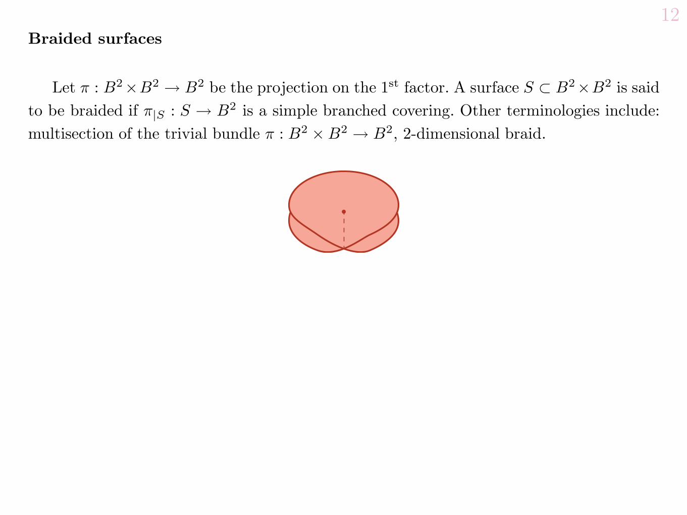
12Braided surfaces
Let ⇧ : B2⇥B2 ⌃ B2 be the projection on the 1st factor. A surface S ⇧ B2⇥B2 is saidto be braided if ⇧|S : S ⌃ B2 is a simple branched covering. Other terminologies include:multisection of the trivial bundle ⇧ : B2 ⇥B2 ⌃ B2, 2-dimensional braid.
The braid monodromy of a degree-d braided surface S with branching set BS ⇧ B2 isa representation ⌃S : ⇧1(B2 �BS)⌃ Bd, with Bd the braid group on d strands.
Fundamental fact: the monodromy of a meridian of BS is a half-twist in the braid group,that is the conjugate to a standard generator (or its inverse).
A half-twist is determined by an arc ⇥ ⇧ B2 between two branch points, and missingthe branch set in its interior. The half-twist t� determined by ⇥ is a homeomorphism withsupport in a small regular neighborhood of ⇥, where it exchanges the two endpoints of ⇥.
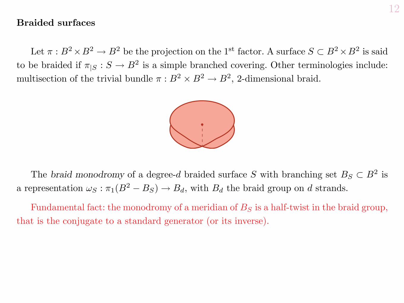
13
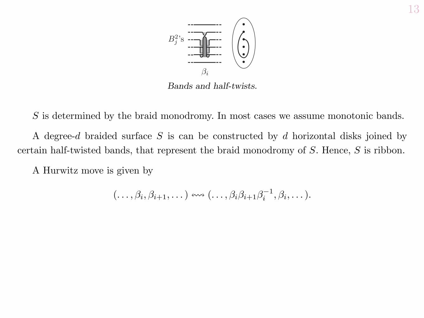
Bands and half-twists.
S is determined by the braid monodromy. In most cases we assume monotonic bands.
A degree-d braided surface S is can be constructed by d horizontal disks joined bycertain half-twisted bands, that represent the braid monodromy of S. Hence, S is ribbon.
Another move is the stabilization (also said Markov stabilization): addition of a trivial2-disk, along with a band connecting it with an existing sheet of S. The new braided surfacehas degree d + 1.
A braided surface with monotonic bands can be easily transformed into a flat diagramof a ribbon surface.
13
Bands and half-twists.
S is determined by the braid monodromy. In most cases we assume monotonic bands.
A degree-d braided surface S is can be constructed by d horizontal disks joined bycertain half-twisted bands, that represent the braid monodromy of S. Hence, S is ribbon.
Another move is the stabilization (also said Markov stabilization): addition of a trivial2-disk, along with a band connecting it with an existing sheet of S. The new braided surfacehas degree d + 1.
A braided surface with monotonic bands can be easily transformed into a flat diagramof a ribbon surface.
14
Flattening of a braided surface.
14
Flattening of a braided surface.
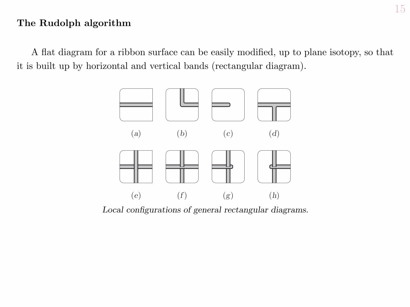
15The Rudolph algorithm
A flat diagram for a ribbon surface can be easily modified, up to plane isotopy, so thatit is built up by horizontal and vertical bands (rectangular diagram).
Local configurations of general rectangular diagrams.
These local configurations are up to rotations by ⇧/2, ⇧, or 3⇧/2 radians such that thebottom left corner is rounded.
First, we restrict to the following special configurations (only few rotations in previousfigure are allowed).
16
Special configurations.
16
Special configurations.
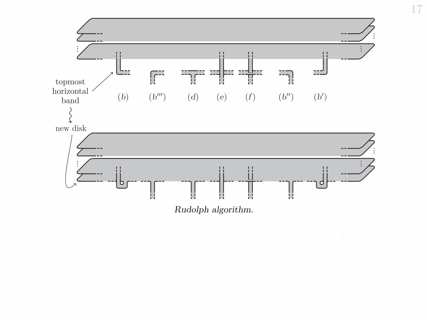
17
Rudolph algorithm.
Now transform each half-curl into a half-twist to get the braided surface (with monotonicbands).
17
Rudolph algorithm.
Now transform each half-curl into a half-twist to get the braided surface (with monotonicbands).
17
Rudolph algorithm.
Now transform each half-curl into a half-twist to get the braided surface (with monotonicbands).
17
Rudolph algorithm.
Now transform each half-curl into a half-twist to get the braided surface (with monotonicbands).
18Then extend to the general case.
From general to special configurations.
We get a standard way to transform each rectangular diagram into a braided surface.
18Then extend to the general case.
From general to special configurations.
We get a standard way to transform each rectangular diagram into a braided surface.
18Then extend to the general case.
From general to special configurations.
We get a standard way to transform each rectangular diagram into a braided surface.
18Then extend to the general case.
From general to special configurations.
We get a standard way to transform each rectangular diagram into a braided surface.
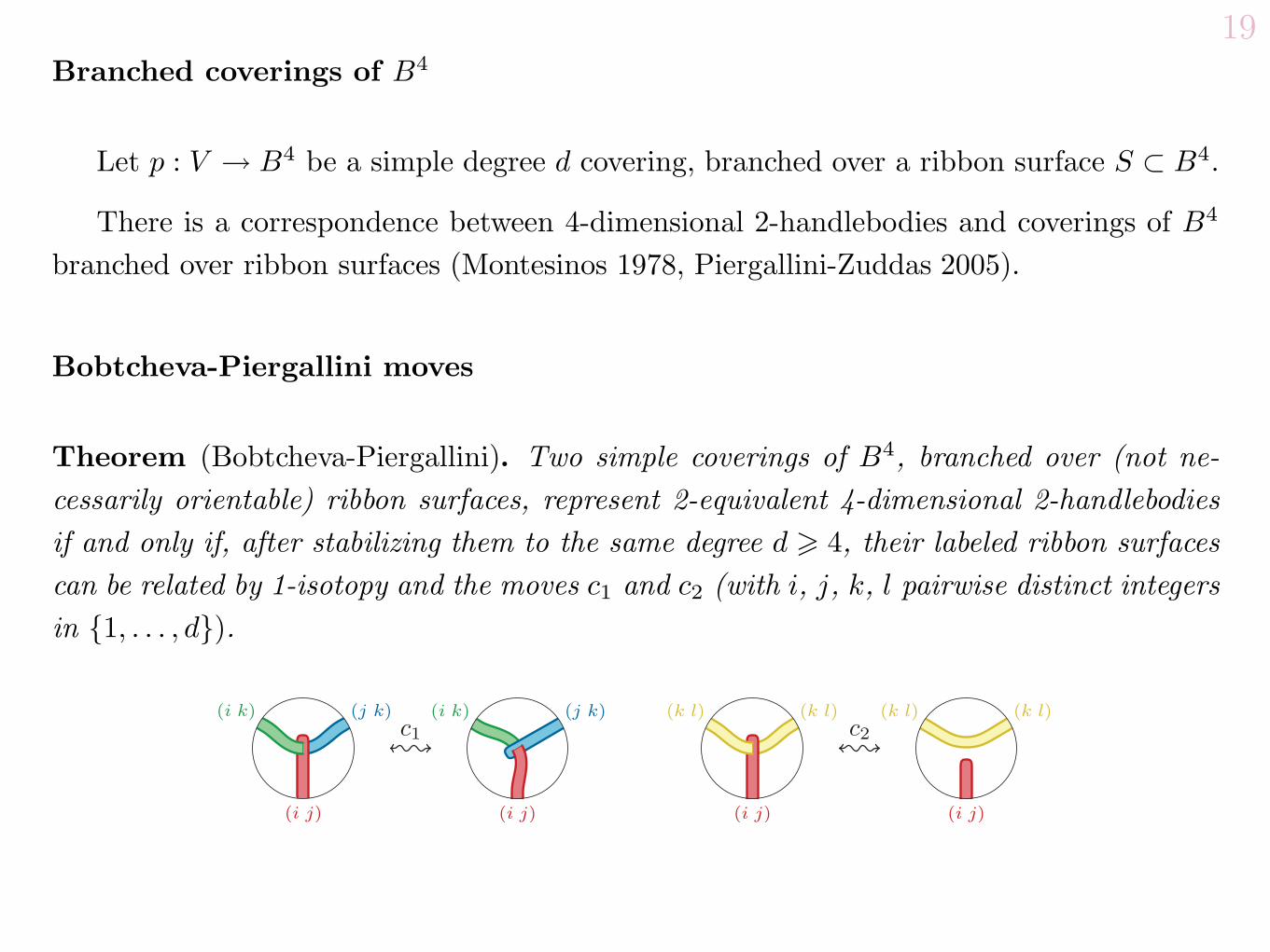
19Branched coverings of B4
Let p : V ⌃ B4 be a simple degree d covering, branched over a ribbon surface S ⇧ B4.
There is a correspondence between 4-dimensional 2-handlebodies and coverings of B4
branched over ribbon surfaces (Montesinos 1978, Piergallini-Zuddas 2005).
Bobtcheva-Piergallini moves
Theorem (Bobtcheva-Piergallini). Two simple coverings of B4, branched over (not ne-cessarily orientable) ribbon surfaces, represent 2-equivalent 4-dimensional 2-handlebodiesif and only if, after stabilizing them to the same degree d ⇤ 4, their labeled ribbon surfacescan be related by 1-isotopy and the moves c1 and c2 (with i, j, k, l pairwise distinct integersin {1, . . . , d}).
20From these moves it is possible to derive the following (the left part is labeled in �d,
while the right part is labeled in �d+1). This is useful to handle the above non-orientabilityissue.
20From these moves it is possible to derive the following (the left part is labeled in �d,
while the right part is labeled in �d+1). This is useful to handle the above non-orientabilityissue.
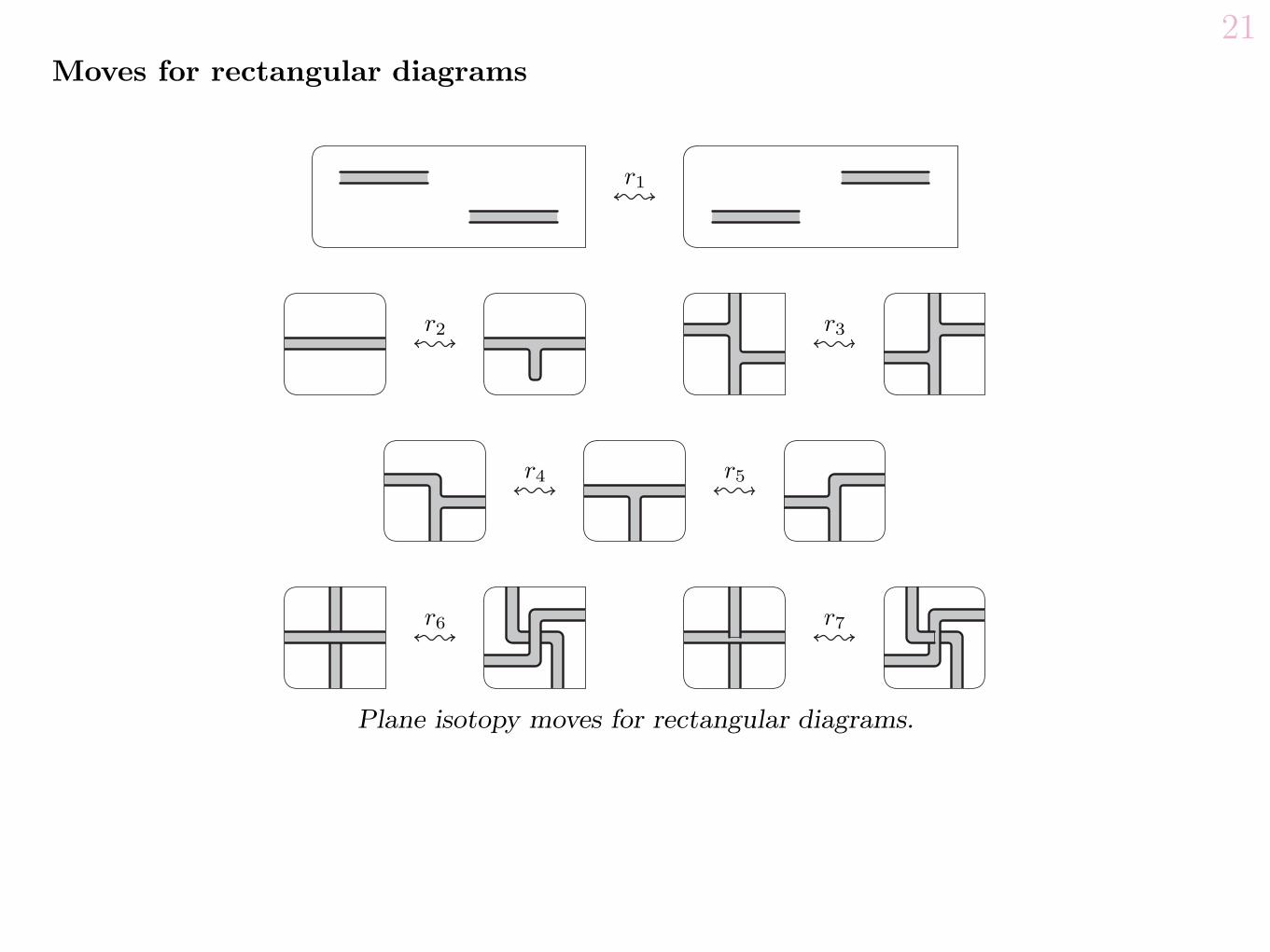
21Moves for rectangular diagrams
Plane isotopy moves for rectangular diagrams.
21Moves for rectangular diagrams
Plane isotopy moves for rectangular diagrams.
21Moves for rectangular diagrams
Plane isotopy moves for rectangular diagrams.
22
3-Dimensional isotopy moves for rectangular diagrams.
22
3-Dimensional isotopy moves for rectangular diagrams.
22
3-Dimensional isotopy moves for rectangular diagrams.
23
1-Isotopy moves for rectangular diagrams.
Covering moves for labeled rectangular diagrams.
23
1-Isotopy moves for rectangular diagrams.
Covering moves for labeled rectangular diagrams.
23
1-Isotopy moves for rectangular diagrams.
Covering moves for labeled rectangular diagrams.
243 Lefschetz fibrations and branched coverings
Let f : V ⌃ B2 be a (allowable) Lefschetz fibration, �F ⌥= ⌥O. There is a simple coveringp : V ⌃ B2 ⇥B2, branched over a braided surface S ⇧ B2 ⇥B2 such that
f = ⇧ ⇤ p,
with ⇧ : B2 ⇥ B2 ⌃ B2 the projection (Z. 2009, also Loi and Piergallini 2001 in case �F
connected).
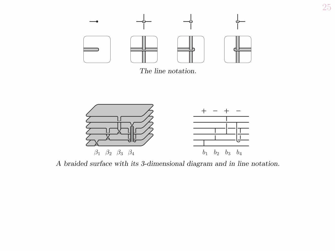
25
The line notation.
A braided surface with its 3-dimensional diagram and in line notation.
25
The line notation.
A braided surface with its 3-dimensional diagram and in line notation.
25
The line notation.
A braided surface with its 3-dimensional diagram and in line notation.
264 Proof of the main theorem
We are going to prove that our moves S± and T generate 2-equivalence. Let f : V ⌃ B2
and f ⇥ : V ⇥ ⌃ B2 be two Lefschetz fibrations on 2-equivalent 4-dimensional 2-handlebodiesV ⌅=2 V ⇥.
Step 0
Up move U we can assume that f and f ⇥ are allowable.
Step 1
Represent f and f ⇥ by branched coverings of B2⇥B2: f = ⇧ ⇤p and f ⇥ = ⇧ ⇤p⇥. We gettwo (monotonic) labeled braided surfaces S and S⇥ that we want to relate in some way.
We can now apply the flattening procedure to get two labeled rectangular diagrams,which we still denote by S and S⇥. Now, we know that S and S⇥ are related by the movesr1 to r25.
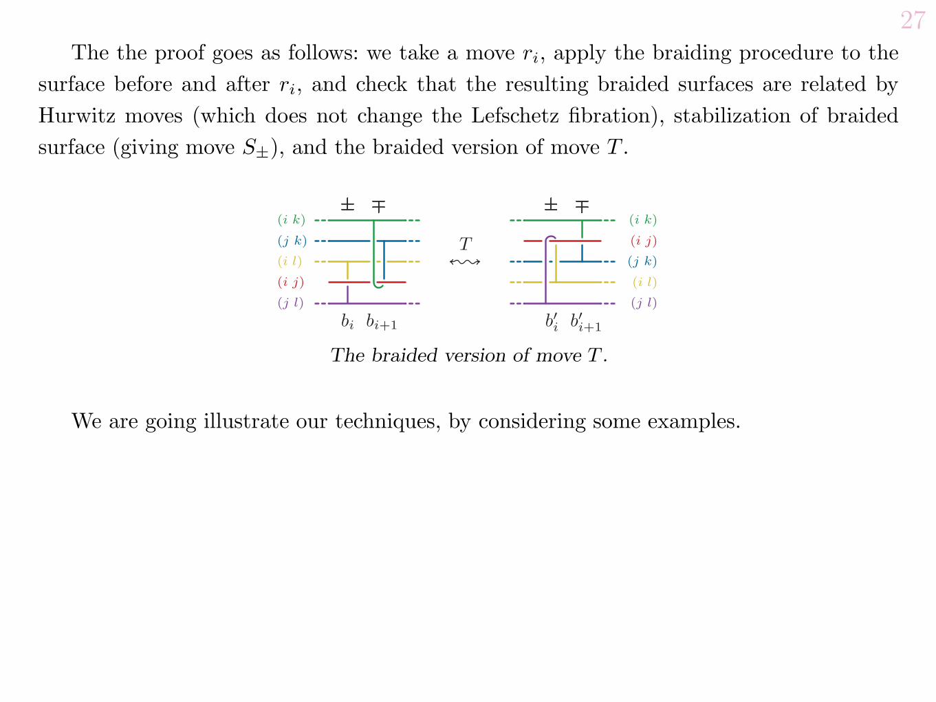
27The the proof goes as follows: we take a move ri, apply the braiding procedure to the
surface before and after ri, and check that the resulting braided surfaces are related byHurwitz moves (which does not change the Lefschetz fibration), stabilization of braidedsurface (giving move S±), and the braided version of move T .
The braided version of move T .
We are going illustrate our techniques, by considering some examples.
28Step 2: braiding rectangular moves
First, we give a trick that will be useful: sliding a band over another. This is nothingbut a special case of Hurwitz moves. In figure are shown the three kind of sliding, both forpositive and negative bands. This plays a central role.
Sliding bands.
A figure in band notation would better clarify what happens.
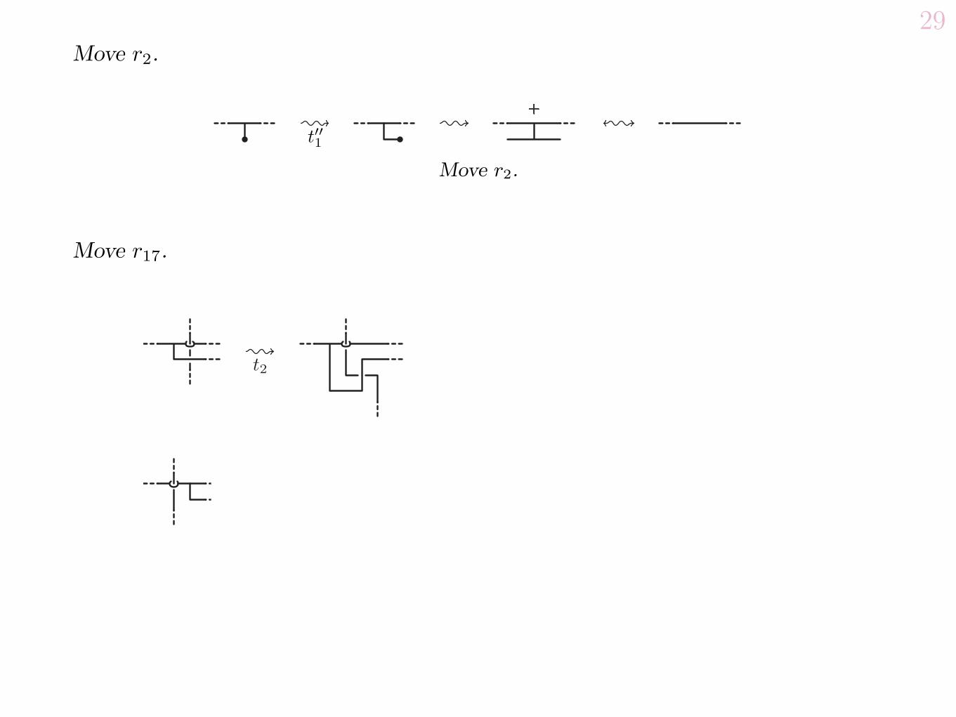
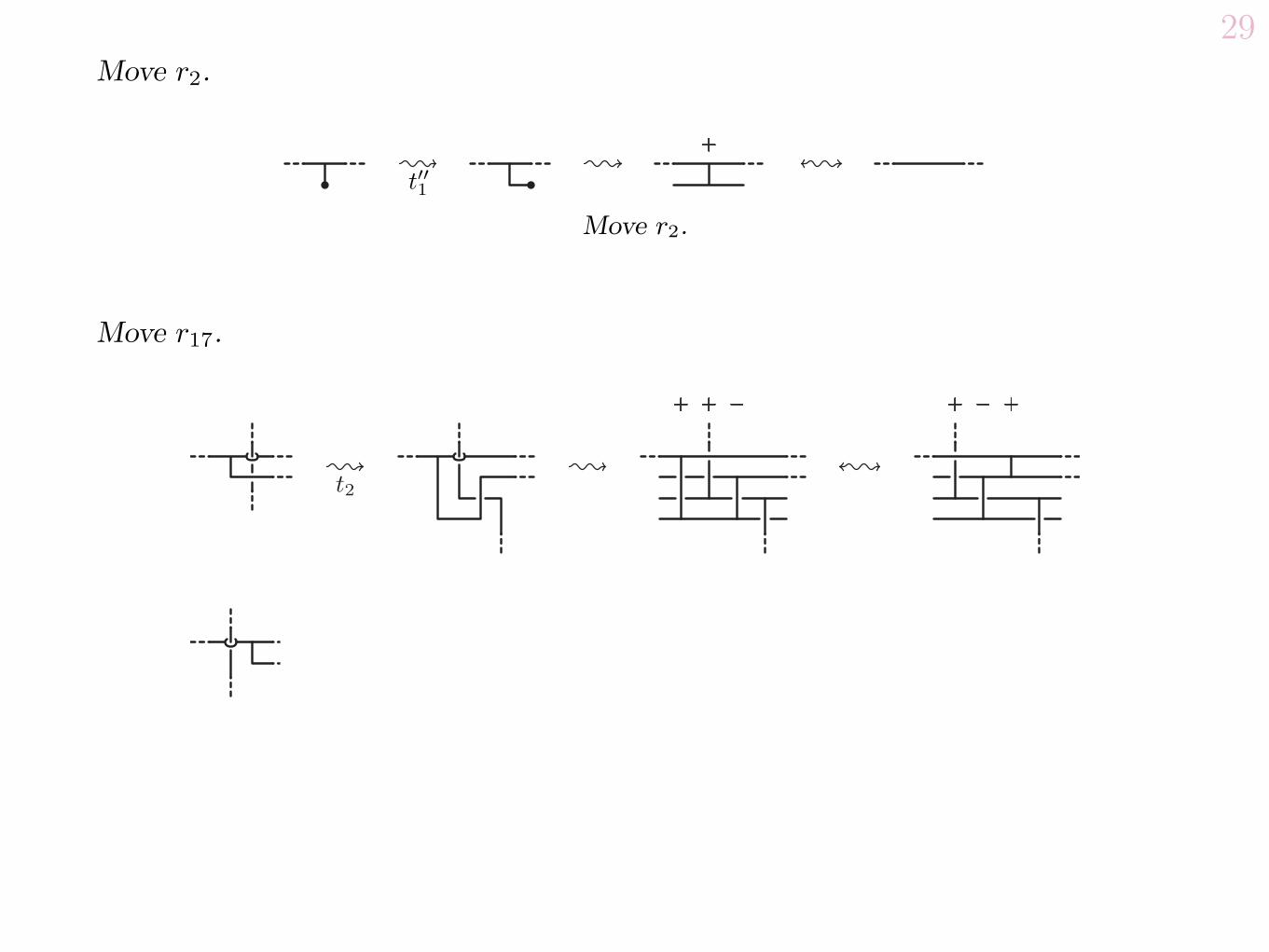
29Move r2.
Move r2.
Move r17.
Move r17.
29Move r2.
Move r2.
Move r17.
Move r17.
29Move r2.
Move r2.
Move r17.
Move r17.
29Move r2.
Move r2.
Move r17.
Move r17.
29Move r2.
Move r2.
Move r17.
Move r17.
29Move r2.
Move r2.
Move r17.
Move r17.
29Move r2.
Move r2.
Move r17.
Move r17.
29Move r2.
Move r2.
Move r17.
Move r17.
29Move r2.
Move r2.
Move r17.
Move r17.
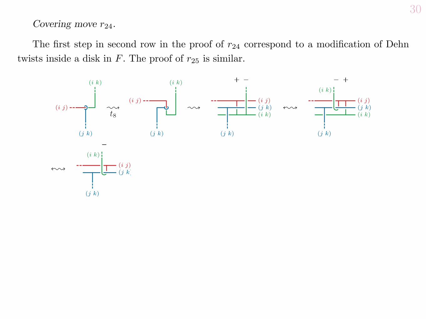
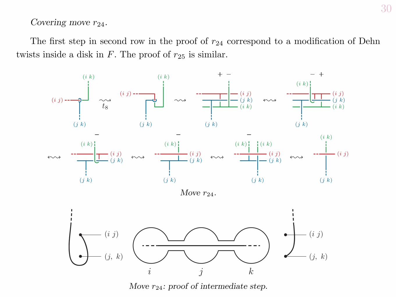
30Covering move r24.
The first step in second row in the proof of r24 correspond to a modification of Dehntwists inside a disk in F . The proof of r25 is similar.
Move r24.
i j k
(i j)
(j, k)
(i j)
(j, k)
Move r24: proof of intermediate step.
30Covering move r24.
The first step in second row in the proof of r24 correspond to a modification of Dehntwists inside a disk in F . The proof of r25 is similar.
Move r24.
i j k
(i j)
(j, k)
(i j)
(j, k)
Move r24: proof of intermediate step.
30Covering move r24.
The first step in second row in the proof of r24 correspond to a modification of Dehntwists inside a disk in F . The proof of r25 is similar.
Move r24.
i j k
(i j)
(j, k)
(i j)
(j, k)
Move r24: proof of intermediate step.
30Covering move r24.
The first step in second row in the proof of r24 correspond to a modification of Dehntwists inside a disk in F . The proof of r25 is similar.
Move r24.
i j k
(i j)
(j, k)
(i j)
(j, k)
Move r24: proof of intermediate step.
30Covering move r24.
The first step in second row in the proof of r24 correspond to a modification of Dehntwists inside a disk in F . The proof of r25 is similar.
Move r24.
i j k
(i j)
(j, k)
(i j)
(j, k)
Move r24: proof of intermediate step.
30Covering move r24.
The first step in second row in the proof of r24 correspond to a modification of Dehntwists inside a disk in F . The proof of r25 is similar.
Move r24.
i j k
(i j)
(j, k)
(i j)
(j, k)
Move r24: proof of intermediate step.
30Covering move r24.
The first step in second row in the proof of r24 correspond to a modification of Dehntwists inside a disk in F . The proof of r25 is similar.
Move r24.
i j k
(i j)
(j, k)
(i j)
(j, k)
Move r24: proof of intermediate step.
30Covering move r24.
The first step in second row in the proof of r24 correspond to a modification of Dehntwists inside a disk in F . The proof of r25 is similar.
Move r24.
i j k
(i j)
(j, k)
(i j)
(j, k)
Move r24: proof of intermediate step.
30Covering move r24.
The first step in second row in the proof of r24 correspond to a modification of Dehntwists inside a disk in F . The proof of r25 is similar.
Move r24.
i j k
(i j)
(j, k)
(i j)
(j, k)
Move r24: proof of intermediate step.
30Covering move r24.
The first step in second row in the proof of r24 correspond to a modification of Dehntwists inside a disk in F . The proof of r25 is similar.
Move r24.
i j k
(i j)
(j, k)
(i j)
(j, k)
Move r24: proof of intermediate step.
30Covering move r24.
The first step in second row in the proof of r24 correspond to a modification of Dehntwists inside a disk in F . The proof of r25 is similar.
Move r24.
i j k
(i j)
(j, k)
(i j)
(j, k)
Move r24: proof of intermediate step.
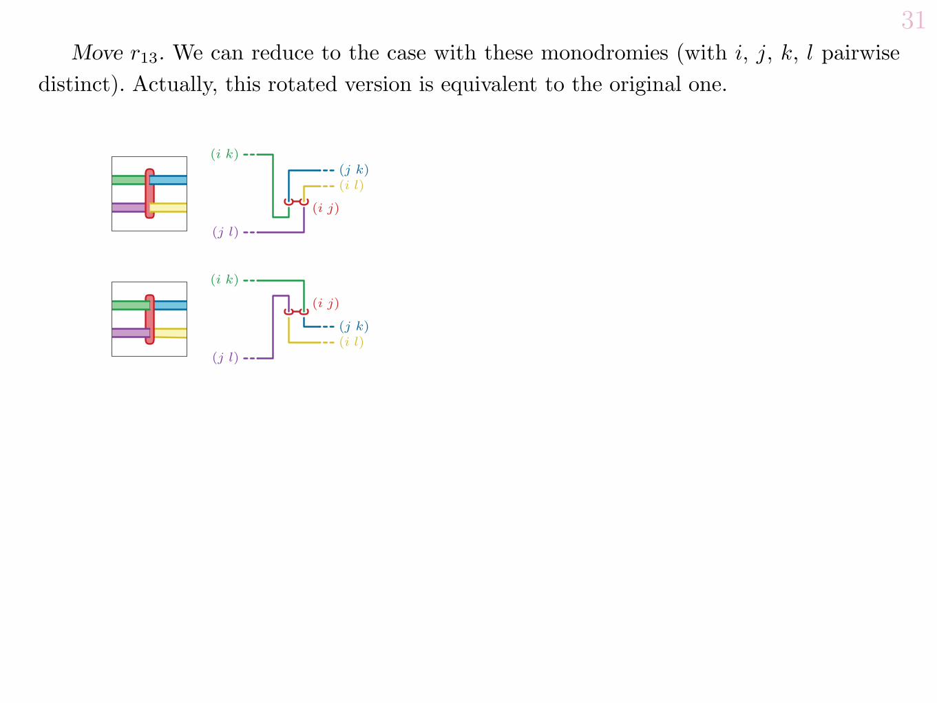
31Move r13. We can reduce to the case with these monodromies (with i, j, k, l pairwise
distinct). Actually, this rotated version is equivalent to the original one.
Move r25.
Thank you for your attention!
31Move r13. We can reduce to the case with these monodromies (with i, j, k, l pairwise
distinct). Actually, this rotated version is equivalent to the original one.
Move r25.
Thank you for your attention!
31Move r13. We can reduce to the case with these monodromies (with i, j, k, l pairwise
distinct). Actually, this rotated version is equivalent to the original one.
Move r25.
Thank you for your attention!
31Move r13. We can reduce to the case with these monodromies (with i, j, k, l pairwise
distinct). Actually, this rotated version is equivalent to the original one.
Move r25.
Thank you for your attention!
31Move r13. We can reduce to the case with these monodromies (with i, j, k, l pairwise
distinct). Actually, this rotated version is equivalent to the original one.
Move r25.
Thank you for your attention!
31Move r13. We can reduce to the case with these monodromies (with i, j, k, l pairwise
distinct). Actually, this rotated version is equivalent to the original one.
Move r25.
Thank you for your attention!
31Move r13. We can reduce to the case with these monodromies (with i, j, k, l pairwise
distinct). Actually, this rotated version is equivalent to the original one.