An Error-Correction Model of U.S. M2 Demand Yash P. Mehra Much applied research in monetary economics has been devoted to the specification of the money de- mand function. Money demand specification has im- portant policy implications. A poorly specified money demand function could yield, for example, spurious inferences on the underlying stability of money demand-a consideration of central importance in the formulation of monetary policy. This paper is concerned with one aspect of money demand specification, namely, the choice of the form in which variables enter the money demand function. It is common to specify the money demand func- tion either in log-level form or in log-difference form. The log-level form, popularized by Goldfeld’s (1974) work, has often been criticized on the ground that the levels of many economic variables included in money demand functions are nonstationary. There- fore, the regression equations that relate such variables could be subject to “the spurious regres- sion phenomenon” first described in Granger and Newbold (1974). This phenomenon, later formal- ized in Phillips (1986), refers to the possibility that ordinary least-squares parameter estimates in such regressions do not converge to constants and that the usual t- and F-ratio test statistics do not have even the limiting distributions. Their use in that case generates spurious inferences. In view of these con- siderations, many analysts now routinely specify the money demand functions in first-difference form. Quite recently, the appropriateness of even the first-difference specification has been questioned. In particular, if the levels of the nonstationary variables included in money demand functions are cointegrated as discussed in Engle and Granger (1987),’ then r Let Xrr, Xzt, and X3t be three time series. Assume that the levels of these time series are nonstationary but first differences are not. Then these series are said to be cointegrated if there exists a vector of constants (or, CY~, (~3) such that Z, = err Xrt + (~7 XT, + CYY~ Xx, is stationarv. The intuition behind this defini- tion is t;at even if-each time series is nonstationary, there might exist linear combinations of such time series that are stationary. In that case, multiple time series are said to be cointegrated and share some common stochastic trends. We can interpret the presence of cointegration to imply that long-run movements in these multiple time series are related to each other. such regressions should not be estimated in first- difference form. This is because level regressions which relate the cointegrated variables can be con- sistently estimated by ordinary least-squares without being subject to the spurious regression phenomenon described above.2 One implication of this work is that money demand functions estimated in first- difference form may be misspecified because such regressions ignore relationships that exist among the levels of the variables. Since there are potential problems with money de- mand functions specified either in level or in first- difference form, some analysts have recently begun to integrate these two specifications using the theories of error-correction and cointegration. In this ap- proach, a long-run equilibrium money demand model (cointegrating regression) is first fit to the levels of the variables, and the calculated residuals from that model are used in an error-correction model which specifies the system’s short-run dynamics.3 Such an approach permits both the levels and first-differences of the nonstationary variables to enter the money de- mand function. This approach also makes it easier to distinguish between the short- and long-run money demand functions. Thus, some variables that are in- cluded in the short-run part of the model might not be included in the long-run part and vice versa, thereby permitting considerable flexibility in the specification of the money demand function. This paper illustrates the use of the above approach by presenting and estimating an error-correction model of U.S. demand for money (MZ) in the postwar period. The money demand function presented here exhibits parameter stability. Money growth forecasts generated by this function are 2 The usual t- and F-ratio statistics can be used provided some other conditions are satisfied and other adjustments are made. See Phillips (1986) and West (1988). 3 This approach, popularized by Hendry and Richard (1982) and Hendry, Pagan and Sargan (1983) has been applied to study U.K. money demand behavior by Hendry and Ericsson (1990) and U.S. money demand behavior by Small and Porter (1989) and Baum and Furno (1990). FEDERAL RESERVE BANK OF RICHMOND 3
Transcript
An Error-Correction Model of
U.S. M2 Demand Yash P. Mehra
Much applied research in monetary economics has been devoted to the specification of the money de- mand function. Money demand specification has im- portant policy implications. A poorly specified money demand function could yield, for example, spurious inferences on the underlying stability of money demand-a consideration of central importance in the formulation of monetary policy.
This paper is concerned with one aspect of money demand specification, namely, the choice of the form in which variables enter the money demand function. It is common to specify the money demand func- tion either in log-level form or in log-difference form. The log-level form, popularized by Goldfeld’s (1974) work, has often been criticized on the ground that the levels of many economic variables included in money demand functions are nonstationary. There- fore, the regression equations that relate such variables could be subject to “the spurious regres- sion phenomenon” first described in Granger and Newbold (1974). This phenomenon, later formal- ized in Phillips (1986), refers to the possibility that ordinary least-squares parameter estimates in such regressions do not converge to constants and that the usual t- and F-ratio test statistics do not have even the limiting distributions. Their use in that case generates spurious inferences. In view of these con- siderations, many analysts now routinely specify the money demand functions in first-difference form.
Quite recently, the appropriateness of even the first-difference specification has been questioned. In particular, if the levels of the nonstationary variables included in money demand functions are cointegrated as discussed in Engle and Granger (1987),’ then
r Let Xrr, Xzt, and X3t be three time series. Assume that the levels of these time series are nonstationary but first differences are not. Then these series are said to be cointegrated if there exists a vector of constants (or, CY~, (~3) such that Z, = err Xrt + (~7 XT, + CYY~ Xx, is stationarv. The intuition behind this defini- tion is t;at even if-each time series is nonstationary, there might exist linear combinations of such time series that are stationary. In that case, multiple time series are said to be cointegrated and share some common stochastic trends. We can interpret the presence of cointegration to imply that long-run movements in these multiple time series are related to each other.
such regressions should not be estimated in first- difference form. This is because level regressions which relate the cointegrated variables can be con- sistently estimated by ordinary least-squares without being subject to the spurious regression phenomenon described above.2 One implication of this work is that money demand functions estimated in first- difference form may be misspecified because such regressions ignore relationships that exist among the levels of the variables.
Since there are potential problems with money de- mand functions specified either in level or in first- difference form, some analysts have recently begun to integrate these two specifications using the theories of error-correction and cointegration. In this ap- proach, a long-run equilibrium money demand model (cointegrating regression) is first fit to the levels of the variables, and the calculated residuals from that model are used in an error-correction model which specifies the system’s short-run dynamics.3 Such an approach permits both the levels and first-differences of the nonstationary variables to enter the money de- mand function. This approach also makes it easier to distinguish between the short- and long-run money demand functions. Thus, some variables that are in- cluded in the short-run part of the model might not be included in the long-run part and vice versa, thereby permitting considerable flexibility in the specification of the money demand function.
This paper illustrates the use of the above approach by presenting and estimating an error-correction model of U.S. demand for money (MZ) in the postwar period. The money demand function presented here exhibits parameter stability. Money growth forecasts generated by this function are
2 The usual t- and F-ratio statistics can be used provided some other conditions are satisfied and other adjustments are made. See Phillips (1986) and West (1988).
3 This approach, popularized by Hendry and Richard (1982) and Hendry, Pagan and Sargan (1983) has been applied to study U.K. money demand behavior by Hendry and Ericsson (1990) and U.S. money demand behavior by Small and Porter (1989) and Baum and Furno (1990).
FEDERAL RESERVE BANK OF RICHMOND 3
consistent with the actual behavior ,of ,M2 growth during the last two decades or.so..A key feature of the results presented here is that consumer spending is found to be a better short-run scale variable than real GNP, even though it is the latter that enters the long-run part of the modeL4
The plan of this paper is as follows. Section 1 presents the error-correction model and discusses the issues that arise in the estimation of such models. Section 2 presents the empirical results. The sum- mary observations are stated in Section 3.
I. AN ERROR-CORRECTION MONEYDEMANDMODEL:.
SPECIFICATION AND ESTIMATION
Specification of an M2 Demand Model
The error-c,orrection money demand model has two parts. The first is a long-run equilibrium money demand function
rM& = aa + al rYt - a2 (R-RM2)t + Ut (1)
where all variables are expressed in their natural logarithms and where rM2 is real M2 balances; rY, real GNP; R, a short-term nominal rate of interest; RMZ, the own rate of return on M2; and U, the long- run random disturbance term. Equation 1 says that the pubhc’s demand for real M2 balances depends upon a scale variable measured by real GNP and an opportunity cost variable measured as the differen- tial between the nominal rate of interest and the own rate of return on M2. The parameters al and aa measure respectively the .long-run income and opportunity cost elasticities. A key aspect of the specification used here is that the own rate of return on M2 is relevant in determining M2 demand (Small and Porter, 1989, and Hetzel and Mehra, 1989). The conventional specification usually omits this variable (see, for example, Baum and Furno, 1990).
The second part of the model is a dynamic error- correction equation of the form
4 The results presented here are in line with those given in Small and Porter (1989) but differ from those given in Baum and Furno (1990). The error-correction model of M2 demand reported in Baum and Furno does not exhibit parameter sta- bility. One possible reason for this is the use of inaoorooriate scale and/or bpportunity cost variables. The money der&dfunc- tion reported in Baum and Furno measures the opportunity cost variable by a short-term market rate of interest, thereby implicitly assuming that the own rate of return on M2 is zero. Further- more, real GNP is used in the long-run as well as in the short- run part of the model.
ArM& = ba”+g~rbr6~ArM2t - s
.n2 + ,FOlas ArYt - s
- ?obsr A(R -RMZ)t - s
+ x Ut-1 +Et (2)
where all variables are as defined above and where et is the. short-run random disturbance term; A,’ the first difference operator; ni(i = 1,2,3), the number of lags; and,.Ut - 1, .‘the lagged value of the long-run random disturbance term. Equation 2 gives the short- run determinants of M2 demand, which include, among others, current and past changes in the scale and opportunity cost variables and the lagged value of the residual from the long-run money demand function. The parameter X that appears on Ut _ 1 in (2) is the error-correction coefficient. At a more intuitive level, the‘ presence of .Ut - I in (2) reflects the presumption that actual Mi balances do not always equal what the public wishes to hold on the basis of the long-run’ factors specified in (1). Therefore, in the short run, the public adjusts its money balances to correct any disequilibrium in its long-run money holdings. The parameter X in (2) measures the role such disequilibria plays in explain- ing the short-run movements in money balances.5
5 It should, however, be pointed out that the size of the coeffi- cient on the error correction variable in (2) is influenced in part by the nature of serial correlation in the random disturbance term of the long-run money demand model and is not necessarily indicative of the speed of adjustment of money demand to its long-run level. To explain it further, for illustrative purposes assume the restricted simple money demand model of the form
m*r = aa + ar yt + Ut (4 where changes in money balances follow the partial-adjustment model
mt - mr-1 =6 (m’r - mr-r), 0 < 6 51 (b) The parameter 6 measures the speed of adjustment. m*. is the long-run desired level of real money balances, and other variables are as defined before. Assume now that the random disturbance term Ur in (a) is stationary and follows a simple AR( 1) process of the form
ut = P u-1 + Et; 0 5 P< 1 (4 The parameter P is determined by the nature of shocks to money demand. Note that the empirical work in the text relies on a long-run demand specification like (a), but allows for more general dynamics than embedded in (b). Equations (a), (b) and (c) imply the following reduced form equation for changes in money balances
mt - mt-r = 6ar Ayt - 6(1-p) Ut-1 + 6 ct. (4 Equation (d) resembles the error-correction model of the form (2) given in the text. As can be seen, the size of the coefficient on the lagged level of Ut depends upon two parameters 6 and P. If P is close to unity, then the error-correction parameter will be small even if 6 is large.
4 ECONOMIC REVIEW, MAY/JUNE 1991
An important assumption implicit in the above discussion is that the random disturbance term Ut is stationary. Intuitively, this assumption means that actual M2 balances do not permanently drift away from what is determined by long-run factors specified in (1). If this assumption is incorrect so that Ut is in fact nonstationary, then the regression equation (I) if estimated is subject to the spurious regression phenomenon. Furthermore, the coefficient X in (2) is likely to be zero. To see this, first-difference the equation (1) as in (3)
ArMZt = al ArYt - a2 A(R -RM&
+ Ut - Q-1 (3)
Assume now that Ut follows a first-order autoregres- sive process of the form
Ut =PUt-1 + Et
where Et is a pure white noise process. Then we can rewrite (3) as in (4)
ArMZt = al ArYt - a2 A(R -RMZ)t
+ (P-1) ut-1 + Et (4)
Equation (4) is similar in spirit to equation (2). If P is less than unity so that Ut is stationary, then P - 1 [which equals X in (Z)] is different from zero. If P = 1 so that Ut is nonstationary, then P - 1 [and X in (Z)] is zero. Hence, the dynamic error-correction specification (2) exists if Ut is a stationary variable.
It can now be easily seen that if Ut is nonstationary, then the money demand regression estimated in first- difference form is appropriate [as X in (2) is in fact zero]. On the other hand, if Ut is stationary, then the first-difference regression is misspecified because it omits the relevant variable Ut - r [as X in (2) is in fact nonzero].
Estimation of the Error-Correction Model
If the random disturbance term Ut is stationary, then the money demand regression (2) can be esti- mated in two alternative ways. The first is a two- step procedure. In the first step, the long-run equilibrium M2 demand model (1) is estimated using a consistent estimation procedure, and the residuals are calculated. In the second step, the short- run money demand regression (2) is estimated with Ut - 1 replaced by residuals estimated in step one (see, for example, Hendry and Ericsson, 1991, and Baum and Furno, 1990). The money demand regression
(5)
estimated in the first step of this procedure generates estimate@ of the long-term income and opportunity cost elasticities (al and az). The short-run money demand parameter estimates are generated in the second step.
The alternative procedure is to replace Ut _ 1 in (2) by the lagged levels of the variables and estimate the short-run and long-run parameters jointly. To explain it further, substitute (1) into (2) to obtain a com- bined equation
ArM& = do +s#lbi, ArM&- s
+ s$ob2s ArYt - s
- szobs, A(R - RM2)t - s
+ di rM&-1 + dz rYt-r
+ ds (R-RMZ)t-1 + et
where do = (bo - ao X)
di = X
dz = -X al
ds = X a2
Equation 5 can be estimated using a consistent estimation procedure and all parameters of (1) and (2) can be recovered from those of (5). For exam- ple, the error-correction coefficient X is di; the long- term income elasticity (al) is dz divided by di; and the long-term opportunity cost elasticity (az) is ds divided by di (see, for example, Small and Porter, 1989).
If one wants to test hypotheses about the long-run parameters of the money demand function (l), it is easier to do so under the second framework than
6 It should be pointed out that if all of the variables included in (1) are nonstationary, then ordinary least squares estimates of (1) are consistent. However, the usual t- and F-ratio statistics have nonstandard limiting distributions because Ur in (1) is generally serially correlated and/or heteroscedastic. This means one can not carry out tests of hypotheses about the long-run parameters in the standard fashion. Furthermore, if even a single variable in (1) is stationary, then ordinary least squares estimates are inconsistent. West (1988) in that case suggests using an in- strumental variables procedure.
FEDERAL RESERVE BANK OF RICHMOND 5
under the two-step procedure.7 The reason is that the residuals in the equilibrium model estimated in step one of the first procedure are likely to be serially correlated and possibly heteroscedastic. Hence, the usual t- and F-ratio test statistics are invalid unless further adjustments are made. In con- trast, the residuals in the money demand regression (5) are likely to be well behaved, validating the use of the standard test statistics in conducting inference. In view of these considerations, the error-correction money demand model is estimated using the second procedure, i.e., the money demand function (5).
As noted above, the long-term income elasticity can be recovered from the long-run part of the model (5), i.e., ai is dz divided by di. It may however be noted that the short-run part of the model (5) may yield another estimate of the long-term scale elas-
ticity, i.e.,szobz./(l -s$lbr,). If the same scale
variable appears in the long- and short-run parts of the model, then a “convergence condition” might be imposed to ensure that one gets the same point- estimate of the long-term scale elasticity. To explain further, assume that real income appears in the long- and short-run parts of the model and that the long- term income elasticity is unity, i.e., al = 1 in (1). This restriction implies that coefficients that appear on rY, - 1 and rM& _ 1 in (5) sum to zero. This restriction pertains to the long-run part of the model and is expressed as in (6.1)
di + dz = 0 (6.1)
Furthermore, if the long-term income elasticity com- puted from the short-run part of the model is unity, then it also implies the following
sfobz.l(l -&bi.) = 1.
Equivalently, (6.2) can be expressed as
sgobzs +s&ls = 1.
(6.2)
7 It should be pointed out that these remarks apply to the case in which the equilibrium model (1) is estimated I& ordinary least sauares. as suegested bv Enele and Graneer (1987). However. if ;he equilibria mane; demand model E estimated using the procedure given in Johansen and Juselius (1989), then one can conduct various tests of hypotheses of the long-run parameters. The approach advanced in Johansen and Juselius is, however, quite complicated.
In general, if different scale variables appear in the short- and long-run parts of the model, then these restrictions may or may not be imposed on the model.
Tests for Cointegration
An assumption that is necessary to yield reliable estimates of the money demand parameters is that Ut in (1) should be stationary. Since the levels of the variables included (1) are generally nonstationary, the stationarity of Ut requires that these nonstationary variables be cointegrated as discussed in Engle and Granger (1987). Hence, one must first test for the existence of a long-run equilibrium relationship among the levels of the nonstationary variables in (1).
Several tests for cointegration have been pro- posed in the literature (see, for example, Engle and Granger, 1987, and Johansen and Juselius, 1989). The test for cointegration used here is the one pro- posed in Engle and Granger (1987) and consists of two steps. The first tests whether each variable in (1) is nonstationary. One does this by performing a unit root test on the variables. The second step tests for the presence of a unit root in the residuals of the levels regressions estimated using the nonstationary variables. If the residuals do not have a unit root, then the nonstationary variables are cointegrated. For the case in hand, if Ut in (1) does not have a unit root, then the nonstationary variables in (1) are said to be cointegrated.
Data and the Definition of Scale Variables
The money demand regression (5) is estimated us- ing the quarterly data that spans the period 1953Q 1 to 1990524. rM2 is measured as nominal M2 deflated by the implicit GNP price deflator; rY by real GNP; R by the four- to six-month commercial paper rate and; RM2 by the weighted average of the explicit rates paid on the components of M2.
The theoretical analysis presented in McCallum and Goodfriend (1987) implies that the scale variable that appears in a typical household’s money demand relationship is real consumption expenditure. Mankiw and Summers (1986) have presented empirical evidence that in aggregate money demand regressions consumer expenditure is a better scale variable than GNP. Their reasoning is based on the observation that some components of GNP, such as business fixed investment and changes in inventories, do not generate as much increase in money balances as does consumer expenditure. The money demand regres- sions estimated. by Ma&w and Summers are in level
6 ECONOMIC REVIEW, MAY/JUNE 1991
form and use distributed lags on the scale and in- terest rate variables. Their empirical work implies that consumer expenditure is a better scale variable than GNP in the short run as well as in the long run. In contrast, Small and Porter (1989) used consumer spending as the short-run scale variable, and GNP as the long-run scale variable. Here I formally test which scale variable is appropriate in the short and long run.*
These results suggest the presence of a single unit rdot in rM&, rYt and rCt, implying chat the levels of these variables are nonstationary but the first- differences are not. The financial market opportunity cost variable (R -RM2)t does not have a unit root and is thus stationary.lO
Cointegration Test Results
II. EMPIRICAL RESULTS
Unit Root Test Results
The money demand regression (5) includes the levels and first-differences of money, income and opportunity cost variables rM&, ArM&, rYt, ArYt, (R - RM& and A(R - RM2)t. The alternative scale variable considered is real consumer expenditure: rCt and ArCt. The Augmented Dickey Fuller test9 is used to test the presence of unit roots in these variables. The test results are reported in Table 1.
The unit root test results presented above imply that except for rM& and rYt all other variables in- cluded in the money demand regression (5) are sta- tionary. If rM& and rYt are cointegrated, then (5) can be estimated by ordinary least squares and the resulting parameter estimates are not subject to the spurious regression phenomenon.
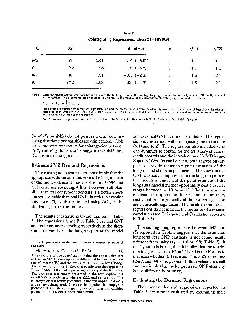
The results of testing for cointegration” between rM& and rYt are presented in Table 2. As can be seen, the residuals from a regression of rM& on rYt
* All the data (with the exception of RMZ and M2) is taken from the Citibank database. M2 for the pre-1959 period and RM2 are constructed as described in Hetzel (1989).
lo Schwert (1987) has shown that usual unit root tests may be invalid if time series are generated by moving as well as autoregressive components. In order to check for this potential bias, unit root tests were repeated using longer lags on first- differences of time series. In particular, the parameter n in Table 1 was set at 8 and 12. Those unit root test results (not reported) yielded similar inferences.
9 The unit root test procedure used here is described in Mehra 11 For a simple description of this cointegration test see Mehra (1990). (1989).
Table 1
Unit Root Test Results, 1953Ql-1990Q4
zt &:p-110)
First Unit Root
p(t:p= 0) a3 (p=l, P=O) n x2(1) x2(2)
rM2,
rYt G (R - RM2),
.97 (-2.2)
.95 (-2.5)
.94 (-2.5)
.80 (-4.2)*
Second Unit Root
.20 (2.0) 2.67 1 .76 1.59
.39 (2.5) 2.50 2 1.50 1.72
.46 (2.5) 3.13 2 .96 1.03
.57 (1.2) 9.07* 4 .37 .42
ArM2, ArYt Arc, A(R - RM2),
.59 (- 5.3)* 1 .28 .39
.31 (-6.5)* 2 .62 1.28
.29 (- 5.3)* 4 .45 .55
.09 (-7.0)* 2 .lO .68
Notes: Regressions are of the form Z, = (I +%zld, AZ,-, + P Z,-, + ,3 T + 4. All variables are in their natural logs; rM2, real balances; rY, real GNP;
rC, real consumer spending; R-RM2, tie differential between the four- to six-month commercial paper rate (RI and the own rate on M2 (RM2); T, a time trend; and A, the first-difference operator. The coefficient reported on trend is to be multiplied by 1000. The parameter n was chosen by the “final prediction error criterion” due to Akaike (1969). The coefficients P and /3 (t statistics in parentheses) are reported. a3 tests the hypothesis 6, 8) = (1,O). 2(l) and ,&2) are Chi square statistics (Godfrey, 1978) that test for the presence of first- and second-order serial correlation in the residuals of the regression.
An “*” indicates significance at the 5 percent level. The 5 percent critical value for t: P - 1=0 is 3.45 (Fuller, 1976, Table 8.5.2) and that for @s:b= 1, fl=O) is 6.49 (Dickey and Fuller, 1981, Table VI).
FEDERAL RESERVE BANK OF RICHMOND 7
x4 x2,
Table 2
Cointegrating Regressions, 1953Q111990Q4
b d (t:d=O) n x*(l) XV)
rM2 rY
rY rM2
rM2 rC
rC rM2
1.01 -.lO l-3.5)* 1 1.1 1.1
.98 -.lO t-3.51* 1 1.1 1.1
.91 -.05 (-2.3) 1 1.6 2.1
1.08 -.05 (-2.3) 1 1.6 2.1
Notes: Each row reports coefficients from two regressions. The first regression is the cointegrating regression of the form Xl, =, a + b X2, + U,, where U, is the residual. The second regression tests for a unit root in the residual of the relevant cointegrating regression and IS of the form
AUr = d U,-, + ; f,AUtTr. s=1
The coefficient reported from the first regression is b and the coefficient d is from the other regression. n is the number of lags chosen by Akaike’s final prediction error criterion. X2(l) and X*(2) are Godfrey (1978) statistics that test for the presence of first- and second-order serial correlation in the residuals of the second regression.
An “*” indicates significance at the 5 percent level. The 5 percent critical value is 3.21 (Engle and Yoo, 1987, Table 3).
(or of rYr on rM2t) do not possess a unit root, im- plying that these two variables are cointegrated. Table 2 also presents test results for cointegration between rM& and rCt; those results suggest that rM& and rCt are not cointegrated.
Estimated M2 Demand Regressions
The cointegration test results above imply that the appropriate scale variable that enters the long-run part of the money demand model (5) is real GNP, not real consumer spending. I2 It is, however, still plau- sible that real consumer spending is a better short- run scale variable than real GNP. In order to examine this issue, (5) is also estimated using ArCt in the short-run part of the model.
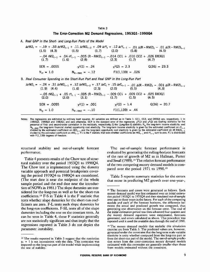
The results of estimating (5) are reported in Table 3. The regressions A and B in Table 3 use real GNP and real consumer spending respectively as the short- run scale variable. The long-run part of the model
r* The long-run money demand functions are assumed to be of the form
rM2t = aa + at rYt - aa (R -RM’&. (1) A key feature of this specification is that the opportunity cost of holding M2 depends upon the differential between a market rate of interest (Rt) and the own rate of return on M2 (RM2t). This specification thus implies that coefficients that appear on Rt and RM2t in (1) are of opposite signs but equal absolute sizes. The unit root test results presented in the text implies that (R-RM2)t is stationary, whereas rM2t and rYt are not. The cointegratjon test results presented in the text implies that rM2t and rYr are cointegrated. These results together then imply the presence of a single cointegrating vector among the variables postulated in (1). See Goodfriend (1990).
still uses real GNP as the scale variable. The regres- sions are estimated without imposing the restrictions (6.1) and (6.2). The regressions also included zero- one dummies to control for the transitory effects of credit controls and the introduction of MMDAs.and Super-NOWs. As can be seen, both regressions ap- pear to provide reasonable point-estimates of the long-run and short-run parameters. The long-run real GNP elasticity computed from the long-run parts of the models is unity, and the point-estimate of the long-run financial market opportunity cost elasticity ranges between - . 10 to - .12. The short-run co- efficients that appear on the scale and opportunity cost variables are generally of the correct signs and are statistically significant. The residuals from these regressions do not indicate the presence of any serial correlation (see Chi square and Q statistics reported in Table 3).
The cointegrating regressions between rM& and rYt reported in Table 2 suggest that the estimated long-term real GNP elasticity is not economically different from unity (ai = 1.0 or .98; Table 2). If this hypothesis is true, then it implies that the restric- tion (6.1) is also true:Fl in Table 3 is the F statistic’ that tests whether (6.1) is true. Fl is .026 for regres- sion A and .44 for regression B. Both ,values are small and thus imply that the long-run real GNP elasticity is not different from unity.
Evaluating the Demand Regressions
The money demand regressions reported in Table 3 are further evaluated by examining their
8 ECONOMIC REVIEW, MAY/JUNE 1991
Table 3
The Error-Correction M2 Demand Regressions, 1953Ql-1990Q4
A. Real GNP in the Short- and Long-Run Parts of the Model
Notes: The regressions are estimated by ordinary least squares. All variables are defined as in Table 1. Ccl, CC2, and D83Ql are, respectively, 1 in 198OQ2, 1980Q3 and 1983Ql and zero otherwise. SER is the standard error of the regression; x2(1) and &2) are Godfrey statistics for the presence of first- and second-order correlation in the residuals, respectively; Q the Ljung-Box Q statistic; N, the long-term income elasticity; and N,-a,, the long-term financial market opportunity cost elasticity. The long-term income elasticity is given by the estimated coefficient on rY,-, divided by the estimated coefficient on rM2,-t and the long-term opportunity cost elasticity is given by the estimated coefficient on (R-RML),-, divided by the estimated coefficient on rM2,-]. Fl is the F statistic that tests whether coefficients on rM2,-, and rY,-, sum to zero. Fl is distributed with F(1,139) degrees of freedom.
structural stability and out-of-sample forecast performance.
Table 4 presents results of the Chow test of struc- tural stability over the period 1953Ql to 199OQ4. The Chow test is implemented using the dummy variable approach and potential breakpoints cover- ing the period 197OQ4 to 198OQ4 are considered. (The start date is near the midpoint of the whole sample period and the end date near the introduc- tion of NOWs in 198 1.) The slope dummies are con- sidered for the long-run as well as for the short-run coefficients.‘3 F-S in Table 4 is the F statistic that tests whether slope dummies for the short-run coef- ficients are zero. F-L tests such slope dummies for the long-run coefficients. F-SL tests all of the slope dummies including the one on the constant term. As can be seen in Table 4, these F statistics generally are not statistically significant and thus imply that the regressions reported in Table 3 do not depict the parameter instability.
13 The results reported in Table 3 suggest that the restriction at = 1 is not inconsistent with the data. This constraint was imposed on the long-run part of the model while implementing the test of stability.
The out-of-sample forecast performance is evaluated by generating the rolling-horizon forecasts of the rate of growth of M2 as in Hallman, Porter and Small (1989). l4 The relative forecast performance of the two competing money demand models is com- pared over the period 1971 to 1990.15
Table 5 reports summary statistics for the errors that occur in predicting M2 growth over one-year-,
1.1 The forecasts and errors were generated as follows. Each money demand model was fist estimated over an initial estima- tion period 19.53521 to 197004 and then simulated out-of-sample over one to three years in the future. For each of the competing models and each of the forecast horizons, the difference be- tween the actual and predicted growth was computed, thus generating one observation on the forecast error. The end of the initial estimation period was then advanced four quarters and the money demand equations were reestimated, forecasts generated, and errors calculated as above. This procedure was repeated until it used the available data through the end of 1990.
1s The money demand models that underlie this simulation exercise are from Table 3. The predicted values are, however, generated under the constraint that the long-term scale variable elasticity is unity whether computed from the long-run part or from the short-run part of the model. The out-of-sample predic- tion errors from the error-correction money demand models estimated with this constraint are generally smaller than those from models estimated without the constraint.
Notes: The reported values are the F statistics that test whether slope dummies when added to equations A and B (reported in Table 3) are jointly significant. The breakpoint refers to the point at which the sample is split in order to define the dummies. The dummies take values 1 for observations greater than the breakpoint and zero otherwise. F-S tests whether slope dummies for the short-run coefficients are zero and are distributed Ft6,131) degrees of freedom. F-L tests whether slope dummies for the long-run coeffi- cients are zero and are distributed Ft2,131) degrees of freedom. F-SL tests whether all of slope dummies including the one on the constant term are zero and are distributed F(9,131) degrees of freedom.
An “*” indicates significance at the 5 percent level.
two-year-, and three-year-ahead periods. Statistics for regression A are shown within brackets. The period-by-period errors are reported only for the M2 demand regression with real consumer spending as the short-run scale variable. These results suggest two observations. The first is that the regression with real consumer spending provides more accurate forecasts of M2 than does the regression with real GNP. For all forecast horizons the root mean squared errors from regression B are smaller than those from regression A (see Table 5). The second is that the error-correction model with real consumer spending as a short-run scale variable does reasonably well in predicting the rate of growth of ML The bias is small and the root mean squared error (RMSE) is 1.0 percentage points for the one-year horizon. Moreover, the prediction error declines as the forecast horizon lengthens.
The out-of-sample M?, forecasts are further evaluated in Table 6, which presents regressions of the form
A t+s = a + b Pt+s, s = 1, ‘2, 3, (7)
where A and P are the actual and predicted values of M2 growth. If these forecasts are unbiased, then a = 0 and b = 1. F statistics reported in Table 6 test the hypothesis (a,b) = (0,l). As can be seen, these F values are consistent with the hypothesis that the forecasts of M2 growth are unbiased.
III. SUMMARY REMARKS
The money demand equations have typically been estimated either in log-level form or in log-difference form. The recent advances in time series analysis have highlighted potential problems with each of these specifications. As a result, several analysts have begun to integrate these two specifications using the theories of error-correction and cointegration. In this approach, a long-run money demand model is first fit to the levels of the variables, and the calculated residuals from that model are used in an error- correction model which specifies the system’s short- run dynamics. Such an approach thus allows both the levels and first-differences of the relevant variables to enter the money demand regression.
Using the above approach, this paper presents an error-correction model of M2 demand in the postwar period. It is shown here that real GNP, not real con- sumer spending, should enter the long-run part of the model. The point-estimate of the long-run real GNP elasticity is not different from unity. Real con- sumer spending however appears more appropriate in the short-run part of the model. The error- correction model with real consumer spending as a short-run scale variable provides more accurate out- of-sample forecasts of M2 growth than does the model with real GNP. However, both of these models are stable by the conventional Chow test over the sample period 1953Ql to 199OQ4.
The out-of-sample forecasts presented here sug- gest that M2 growth in the 1980s is well predicted by the error-correction model that uses real consumer spending as a short-run scale variable. The rate of growth in real consumer spending, which averaged 3.97 percent in the 1983 to 1988 period, decelerated to 1.2 percent in 1989 and 2 percent in 1990. The rate of growth in M2 has also decelerated over the past two years. The money demand model presented here implies that part of the recently observed deceleration in M2 growth reflects deceleration in real consumer spending and is not necessarily indicative of any instability in M2 demand behavior.
Notes: Actual and predicted values are annualized rates of growth of M2 over 4Q-to-4Q periods ending in the years shown. The predicted values are generated using the money demand equation B of Table 3. (See footnote 14 in the text for a description of the forecast procedure used.) The predicted values are generated under the constraint that the long-term scale variable elasticity is unity whether computed from the long-run part or from the short-run part of the model.
a The values in brackets are the summary error statistics generated using the money demand regression A of Table 3.
Notes: The table reports coefficients (standard errors in parentheses) from regressions of the form At,, = a+b Pr,,, where A is actual M2 growth; P predicted M2 growth; and s f= 1,2,3) number of years in the forecast horizon. The values used for A and Pare from Table 5. F3 is the F statistic that tests the null hypothesis ta,b)=(O,l), and are distributed F with degrees of freedom given in parentheses following F3.
FEDERAL RESERVE BANK OF RICHMOND 11
REFERENCES
Akaike, H. “Fitting Autoregressive Models for Prediction.” Annals of Intem&mal S&bics and Mathmatics 2 1 ( 1969): 243-47.
Baum, Christopher F. and Marilena Furno. “Analyzing the Stability of Demand for Money Equations via Bounded- Influence Estimation Techniques.” Journal of Money, Credi and Bat&g (November 1990): 465-7 1.
Dickey, David A. and Fuller, Wayne A. “Likelihood Ratio Statistics for Autoregressive Time Series with a Unit Root.” IGonotnemico 49 (July 1981): 1057-72.
Engle, Robert F. and Byund Sam Yoo. “Forecasting and Testing in a Cointegrated System.” Joamal of Econometrics 35 (1987): 143-59.
Engle, Robert F. and C. W. J. Granger. “Cointegration and Error-Correction Representation, Estimation, and Testing.” Economem~a (March 1987): 25 l-76.
Fuller, W. A. Introduction to Statistical Time Series, 1976, Wiley, New York.
Godfrey, L. G. “Testing for Higher Order Serial Correlation in Regression Equations When the Regressors Include Lagged Dependent Variables.” Econometrica 46 (November 1978): 1303-10.
Goodfriend, Marvin. “Comments on Money Demand, Expec- tations and the Forward-Looking Model.” Journal of Policy Modeling 12(Z), 1990.
Granger, C. W. J., and P. Newbold. “Spurious Regressions in Econometrics.” Journalof EconomemiGs (July 1974): 11 l-20.
Hallman, Jeffrey, J., Richard D. Porter, and David H. Small. “MZ Per Unit of Potential GNP as an Anchor for the Price Level.” Staff Study #157, Board of Governors of the Federal Reserve System (April 1989).
Hendry, D. F. and N. R. Ericsson. “An Econometric Analysis of UK Money Demand in Monetary Trends in the United States and the United Kingdom,” by Milton Friedman and Anna J. Schwartz. American Economic Review (March 1991): 8-38.
Hendry, David F., Adrian R. Pagan, and J. Denis Sargan. “Dynamic Specification.” In Handbook of Econometn&, edited by 2. Griliches and M. Intriligator. Amsterdam: North Holland, 1983.
Hendry, David F., and Jean-Francois Richard. “On the Formu- lation of Empirical Models in Dynamic Econometrics.” Journal of Econometrh 20 (1982): 3-33.
Hetzel, Robert L. “MZ and Monetary Policy.” Federal Reserve Bank of Richmond, l&no& Rti 75 (September/October 1989): 14-29.
Hetzel, Robert L., and Yash P. Mehra. “The Behavior of Money Demand in the 1980s.” J&ma~ of Money, Credit and Banking, (November 1989): 45.5-63.
Johansen, Soren and Katrina Juselius. ‘The Full Information Maximum Likelihood Procedures for Inference on Cointe- grating-with Application.” Institute of Mathematical Sta- tistics, University of Copenhagen, Reprint No. 4, January 1989.
Mankiw, N. Gregory and Lawrence H. Summers. “Money Demand and the Effects of Fiscal Policies.” Journal of Money, &dir and Banking (November 1986): 415-29.
McCallum, Bennett T. and Marvin S. Goodfriend. “Demand for Money: Theoretical Studies.” In T/re New Palgave. A Dictionary of Economics edited by John Eatwell, Munay Milgate, and Peter Newman. Vol. 1, 1987, 775-81.
Mehra, Yash P. “Real Output and Unit Labor Costs as Predictors of Inflation.” Federal Reserve Bank of Richmond, Economic Rezie~~ 76 &rIy/August 1990): 31-39.
. “Some Further Results on the Source of Shift in Ml Demand in the 1980s.” Federal Reserve Bank of Richmond, Econwnic Review 75 (September/October 1989): 3-13.
Phillips, P. C. B. “Understanding Spurious Regressions in Econometrics.” JoumaL of Econometrics 33 (1986): 3 1 l-40.
Schwert, G. W. “Effects of Model Specification on Tests for Unit Roots in Macroeconomic Data.” J&ma/ of Monetaty Economics 20 (1987): 73-103.
Small, David H. and R. D. Porter. “Understanding the Behavior of M2 and VZ.” FederaI Reserve Btdktin (April 1989): 244-54.
12 ECONOMIC REVIEW, MAY/JUNE 1991
A Total Production Index for Washington, D.C.
Dan M. Bechter, Zol’tan Kenessey, Fred Siegmund, and Ray D. Whitman ’
Introduction
This article describes the methods and procedures used in computing a new total production index for the District of Columbia.’ The new index accounts for changes in services production as well as goods production.2 The index made its public debut in a release issued March 15, 199 1, by the Center of Economic and Business Statistics of the University of the District of Columbia. That same day, The Washington Post featured the new index on the first page of its business section. In subsequent months, the Center has issued updates of the index under the release’s name, D.C. Economy.
At the national level, a monthly production index provides a timely measure of cyclical changes in economic output between calendar quarters. Quarterly figures for gross national product provide the most comprehensive measures of production; be- tween quarters, the monthly index of industrial pro- duction compiled by the Federal Reserve Board has proved to be an important and carefully watched economic indicator.
At the regional level, timely measures of output are valuable to business and government officials because economic activity in any region can differ
l Dan Bechter is a vice president at the Federal Reserve Bank of Richmond, Zoltan Kenessey is a senior economist at the Board of Governors of the Federal Reserve System, Fred Siegmund is a professor at the University of the District of Columbia, and Ray Whitman is a professor and the director of the Center of Economic and Business Statistics at the University of the District of Columbia. The views expressed are those of the authors and should not be attributed to the Federal Reserve or to the University of the District of Columbia.
r The “Total Production Index for the District of Columbia” is computed by the Center for Business and Economic Statistics of the University of the District of Columbia and was developed by the Center in cooperation with the Federal Reserve Bank of Richmond and from the experience and advice from staff at the Federal Reserve Board in Washington. The work has been facilitated by an advisory panel consisting of economists from each of these organizations, who met from time to time to review progress on the project. The authors thank Tapas Ghosh for valuable research assistance.
2 The measurement of services production draws heavily on earlier work by Zoltan Kenessey. See, in particular, Kenessey (May 1988; November 1988).
significantly from the national average,and because gross state product figures are available only after a long delay. Output indexes compiled by the Federal Reserve Banks have helped meet the demand for regional economic information used in analyzing economic growth and business cycles, and in economic policy formulation. The attention given to the Federal Reserve’s Beige Book is one example of the interest of policymakers and the public in reports on economic activity around the country.
The District of Columbia economy is different in composition from the economies of surrounding states and the nation as a whole. For example, the government-based D.C. economy has a relatively small manufacturing sector. Manufacturing indexes for Maryland and Virginia therefore provide little guidance about the current state of economic ac- tivity in the nation’s capital. The D.C. economy also behaves differently, although it is not always as insulated from the national business cycle as is com- monly believed. For example, although employment remained relatively flat in the District of Columbia during the U.S. recession of 1974-75, it declined by a larger percentage than U.S. employment over the two recessions of the early 1980s. Also, the booms associated with the D.C. metropolitan area have been much less evident in the city itself. In the past 20 years, for example, employment in the District of Columbia has grown only 20 percent, in contrast to the 89 percent increase in the entire Washington metro area. It is clear, therefore, that although economic activity in the District of Columbia is usually less volatile than in the nation as a whole, it does change in intensity and, sometimes, direction.
Many individual economic indicators are used to help track the D.C. economy. The Washington Post, for example, regularly features charts and data for several different economic sectors. It is difficult to extract from them, however, a clear sense of the general condition and direction of the economy of the District of Columbia. That is, no single indicator fits the pieces of the Washington economy together in a coherent fashion. A timely monthly index of total production does that.
FEDERAL RESERVE BANK OF RICHMOND 13
Background on Production Indexes
The definitive history of production indexes has yet to be written. More than 60 years ago, however, Arthur Burns referred to the European production indexes by Neumann-Spallart of 1887 and Armand Julin of 19 11, and to William Leonard’s 19 13 index dealing with extractive industries in America (Burns, 1930).
The Federal Reserve System has a long history of involvement in the measurement and analysis of monthly production developments. From its first issue in 19 15, the Federa/ Reserve B.&e& contained business conditions data, including some on produc- tion. After January 1919, the Bulletin reported, in more extended form, monthly data on the “physical volume of trade” (including production). The Federal Reserve Board introduced indexes of production in the Buh’etin in the spring of 1922, and in more refined form in the winter of the same year (Federal Reserve Board, March 1922 and December 1922).
Work on indexes of production was also underway outside of the Federal Reserve. Wesley C. Mitchell published an annual index number of production in 1919 (Mitchell, 1919). Mitchell and others at the National Bureau of Economic Research (NBER, incorporated in 1920) played a continuing role in U.S. macroeconomic measurement throughout the 1920s and 1930s and greatly influenced the development of production estimates in general. At Harvard University, Edmund Day produced the Harvard- Census index, also called the Day-Thomas index, by using quinquennial Census of Manufacturers data to adjust annual production indexes (Day, 1920). Walter Steward, who earlier worked at the War Pro- duction Board (led by Mitchell) and who became the director of research at the Federal Reserve Board in 1922, was among those who published articles about production index numbers in those days. During the 192Os, the U.S. Department of Commerce also issued various physical volume data and indexes of output, similar to those in the Fe&al Reserve BuL&irz, which it published in the Surwey of Curt Bushzess.
In 1927 the Federal Reserve Board introduced a new index of industrial production (back to 1919), which can be deemed the beginning of the more elaborate and advanced work on the subject in the United States.3 The index was extensively revised
J Industrial Pmduchn, With a Dexription of the Met/ldoologv, Board of Governors of the Federal Reserve Svstem. 1986. pp. 17-162.
in 1940, 1953, 1959, 1971, 1976, 1985, and most recently in 1989. Over the decades, the Federal Reserve established its preeminent role in monthly industrial output indexes (Federal Reserve Board, 1986). Meanwhile, important research efforts were made elsewhere, notably at the NBER. The work by Arthur Burns, Frederick Mills, Solomon Fabri- cant and others influenced not only the way industrial production was estimated, but also how all other com- ponents of the gross national product were measured.
The basic conceptual issues on production indexes developed by the Federal Reserve have been applied with some adaptations for use in specific regional economies. Regional production indexes compiled by the Federal Reserve Banks, principally for manufacturing, go back to the 195Os, with the earliest attempts undertaken at Atlanta, San Francisco, and Dallas. Today the Midwest Manufacturing Index of the Federal Reserve Bank of Chicago, the Mid- Atlantic Manufacturing Index of the Federal Reserve Bank of Philadelphia, the Fifth District Manufactur- ing Index of the Federal Reserve Bank of Richmond, and the Texas Industrial Production Index of the Federal Reserve Bank of Dallas command interest at the regional level among circles in business, government and academia (Kenessey, 1990).
Nationally, economic policymakers want informa- tion about developments in the various sectors and parts of the country. The uneven behavior of regional economies in recent economic expansions and con- tractions has heightened interest in this kind of information. State and local officials, many of whom are currently faced with budgetary shortfalls, clearly need better information about trends in their area economies. Consumers (and workers) also care a great deal about economic conditions affecting them; the popularity of state and metropolitan business magazines, business journals, and newspaper business sections attests to the public interest in local economic news. To help supplement the supply of state and regional economic information, the Federal Reserve Bank of Richmond calculates and publishes indexes of manufacturing output for each of the five states in the Fifth District (Bechter, et al., 1988).4 Now, the total output index for the District of Columbia, reviewed here, is available.
Production indexes are coincident, not anticipatory, indicators of economic activity. Nationally, the
4 The Fifth Federal Reserve District comprises Maryland, North Carolina, South Carolina, Virginia, most of West Virginia, and the District of Columbia. The manufacturing index for Maryland incorporates the estimate for the District of Columbia.
14 ECONOMIC REVIEW, MAY/JUNE 1991
index of industrial production is one of the four key coincident economic indicators used in identifying peaks and troughs of business cycles. Regionally, production indexes can be used similarly to provide important confirmatory evidence about the current status of output developments in particular economic areas. Regional production indexes are typically used for comparing the performance of a state or area economy with the national total and with other regions. Such analysis, whether it focuses on per- formance over time or across areas, usually high- lights the movements observed for the most recent periods (months or quarters) in a region’s economic activity. Importantly, improved regional measures of output may provide new leading indicators for swings in U.S. economic activity, as some regions may lead (and others lag) national business cycle developments.
The Concept of a Production Index
A production index is an index of the quantity of output, free of any influence of month-to-month changes in prices. 5 The focus on quantity pre- cludes an index that compares current with past dollar values of production, as such an index would measure changes in prices and production together, not just changes in production. One alternative would be to measure production in constant dollars. Such an approach, however, would require a monthly set of price deflators for each product or product group. It seems useful, therefore, to adopt a methodology that relies mainly on physical measures of produc- tion such as tons of coal or taxi miles. Such physical measures of output do not require deflation to eliminate the effect of price changes. Along with the application of proper weights for aggregation, a pro- duction index covering several products can be estimated for each month in a timely fashion.
s It is usually fairly easy to measure the change in output of a single homogenous agricultural or industrial commodity, such as bushels of #l grade durum wheat, or tons of low sulphur bituminous coal. It is quite another matter, however, even when good data are available, to arrive at a “correct” measure of change in overall production when several commodities or grades of commodities are involved. The problem of adding apples and oranges is usually addressed in an economically appealing fashion by using constant prices along with the dollar values of output in some reference period. But because the reference period is usually fixed for a time, measures of change in overall production are plagued by index number problems- for example, the sensitivity of all index numbers to the choice of weights used in the weighted average. The problem in measuring production or prices intertemporally is further com- plicated by changes in the types and qualities of items in the “market basket” over time. These problems are addressed elsewhere in the literature on index numbers.
Most production indexes are of the Laspeyres (base-weighted) type. A Laspeyres quantity index can be expressed as:
It = ig lqitpio
if lqioPio
=iE,qit( pio
iz,qiopio
)
) = iF, ~ Wio
where the summation is over the N individual goods and services included in the index, q denotes the quantities produced of these items, p denotes a term-usually price-used in weighting items in the index, t refers to the current period and o refers to the base period. The weight, wjo, assigned to the jth item and term qjt/qio in the right side of the for- mula, is that item’s share of the value of total output in the base period, or ~opjo/Cqiopio. The weights are held constant over a period of several years until changes in the relative importance of the various items of production have become so extensive that a revision of weights is warranted. Given its con- stant weights, the production index changes over time, as it should, only with changes in the output of goods and services.
As the right side of the formula shows, a quantity index covering several items can be expressed as a weighted average of the production indexes for indi- vidual items. The item weights, or product shares of the base period value of output, add up to 1. The individual and overall quantity indexes are usually ex- pressed as percentages, with 100 the value for the base year.
Application to the District of Columbia
To formulate a production index for the District of Columbia, it was first necessary to decide how much productive activity to include. An index of manufacturing output alone was not likely to be very informative; in the District of Columbia, manufac- turing consists largely of printing and publishing and is a small share of total employment, personal in- come, or production. In the District of Columbia, therefore, where the services-producing sectors dominate economic activity much more than in most of the rest of the country, it was appropriate to design an index of total production to include all significant segments of the economy: communications, con- struction, manufacturing, public utilities, public
FEDERAL RESERVE BANK OF RICHMOND 15
administration, services, trade, transportation, finance and real estate.6
Ideally, a total production index for the District of Columbia (referred to hereafter as the DC index) would draw on a broad range of physical output measures that fit neatly into the categories of the Standard Industrial Classification (SIC). In practice, ideal data series are not available. In the District of Columbia, several different agencies compile data for monthly use, and while many of these data do fit into the SIC categories, others do not. Moreover, as there are tens of thousands of different goods and services being produced, it was not practical to try to include all of them explicitly in the index. Instead, selected items of production were chosen to repre- sent the monthly changes ,in output in various sectors. In selecting representative indicators, an effort was made to include one or more series for each major field of production.
Unfortunately, data on physical units of produc- tion were available for only one-sixth of total pro- duction, as measured by gross product in the base year. Fortunately, the theory of production suggests an alternative way to estimate physical output in the absence of these data. According to production theory, which has ample empirical support in the literature (e.g., the Cobb-Douglas production func- tion), physical units of output can be expressed as a function of physical units of inputs. Moreover, over relatively short periods of time, a production func- tion can be assumed stable, and the inputs of capital and land can be assumed fixed, with production varying with changes in labor input. Together with benchmark information on output provided by gross product data, therefore, labor input data provide a method to interpolate and extrapolate monthly estimates of production.’
Thus, to help construct the DC index where product series were deficient, employment data were used, alone as proxies for quantity series, or as supplements to incomplete quantity series. For example, to measure the production of construction in progress, construction-worker hours are used along with building permits to capture the ongoing nature
6 Quantifying the output of services can present problems, but is often easier than it might seem at first blush. Haircuts are an obvious measure of barber production, for example, and court cases might be used to index the output of lawyer services.
7 The manufacturing output indexes created by the Federal Reserve Bank of Richmond use two inputs, employment and electrical power usage, to estimate changes in output. Whiie both are input measures, they are accounted for in physical units, just as is the production series, rather than in monetary terms.
of the work. Fortunately, labor data are available for all significant productive activities, so employment or production-worker hours by industry can be used as input proxies for production.
When the use of labor is applied as a proxy for production, some account must be made for changes in labor productivity over time. To adjust for the rise in productivity, past increases in average productivity are extrapolated from changes calculated between the most recent years reported by the Bureau of Economic Analysis in its gross product figures for the District of Columbia. For example, if between 1980 and 1986 the change in output of a certain good was 10 percent higher than the change in its labor input, then the average annual increase in labor productivity in the years since was about 1.6 percent, and the monthly increase was therefore assumed constant at about 0.13 percent.
In view of the federal government’s very large share (36 percent in 1986) of productive activity in the economy of the District of Columbia, productivity movements of government workers are of particular interest for estimating output changes in the area. Fortunately, an extensive effort by the U.S. Bureau of Labor Statistics (BLS) within the framework of the Federal Productivity Measurement System (FPMS) produced quantitative results relevant to this topic (BLS, 1990). For fiscal year 1988, for ex- ample, FPMS covered 342 organizations within 61 federal agencies representing 2.1 million persons, 69 percent of the executive branch civilian work force. About 3,000 different products and services were measured in the system. The majority of the 28 major governmental functions, which compose total govern- mental activity reviewed, were services-producing areas. Yet, BLS was able to find representative product measures for these areas just as for goods- producing activities.
The BLS study found that output per employee increased at an average annual rate of 1.4 percent in the 1967-88 period and 0.7 percent between 1983 and 1988. This finding suggests that the usual assumption of unchanged productivity of federal employees in estimating government output is untenable. In the context of the DC index, the BLS results provide the productivity factors necessary for estimating output changes in an important segment of the economy. Moreover, future refinements of the DC index may draw on the FPMS experience. The various government product series that the FPMS identified could be utilized to estimate monthly production directly on the basis of output data rather
16 ECONOMIC REVIEW, MAY/JUNE 1991
than indirectly via labor proxies related to inputs. Thus, the large percentage share of labor-based series could be reduced and the number of product series increased in the DC index.
In several instances, production indexes are cur- rently represented in the DC index both by an output series and by an input (employment) series. Rail transportation production, for example, is represented both by the number of AMTRAK passengers and by hours worked by railroad employees; telephone production is represented both by the number of business calls and by communica- tions employment; and so on. When an activity is represented by two series, the SIC weight is split on the basis of their relative significance or in 50-50 proportion between the output series and the labor series, respectively.
The DC index is adjusted for workdays and seasonal variations. Workdays within any month vary from year to year, and seasonal variations occur as well. In making the workday adjustments, it was necessary to establish a normal workweek for each production category. Hotels, for example, do not normally close on weekends, while many retail or banking establishments close on Sundays or perhaps on both Saturday and Sunday.
The DC index is a base-period weighted, Laspeyres-type index. Individual production indi- cators were assigned weights based on their shares of total value added in 1986, the most recent year for which gross state product data are available. The value-added weights are derived from the 1986 Gross State Product figures published by the Bureau of Economic Analysis of the U.S. Department of Commerce.
Results
The seasonally adjusted values for the DC index over the past four years are charted here along with the seasonally adjusted values of the U.S. Index of Industrial Production (Chart 1). The DC index shows the behavior of total production in the District of Columbia since early 1989 to have been quite dif- ferent from the behavior of U.S. industrial production.
Total production in the District of Columbia grew (on a December-to-December basis) at a rate of 4.0 percent in 1988, 1.2 percent in 1989, and 1.1 per- cent in 1990 despite its essentially flat path over most of that year. Chart 1 indicates that, according to the DC index, the economy of the District of Columbia
Chart 1
INDEXES OF PRODUCTION D.C. Total vs U.S. Industrial
113r 111
109 107
105
103
101
99
97 95 1 I
1987 1988 1989 1990
slowed in 1989, peaked in January 1990, showed no clear trend through December 1990, and rose in early 199 1. It should be noted that the index reflects in- creases in labor productivity assumed in connection with measuring some output components by using labor data proxies.
The DC index covers all goods- and service- producing industries included in the Standard In- dustrial Classification. Normally, production is classified into four major areas: primary production (agriculture and mining), secondary production (manufacturing and construction), tertiary production (transportation, communications, utilities, retail and wholesale trade), and quaternary production (finance, insurance, and real estate, services and public ad- ministration). In the DC index, however, production is classified in three areas-goods, tertiary services, and quaternary services-because primary produc- tive activity (agriculture and mining) is virtually nonexistent in the District of Columbia. Separate tabulations are made also for a total services index which combines tertiary and quaternary production, a private sector index which includes everything but government (federal and local) production, and a public sector index that includes only federal and local government activity. The appendix to this article tabulates the monthly values for all of these indexes from January 1987 through early 1991 (Table 5).
In the DC index, goods production accounts for about 11 percent of total production. This 11 per- cent is divided mainly between construction (7.1 per- cent) and printing and publishing (2.6 percent).
FEDERAL RESERVE BANK OF RICHMOND 17
Goods production has been volatile in recent years and has exhibited some weakness since late 1988. Chart 2 compares the behaviors of the DC index goods component with the Maryland-D.C. index of manufacturing compiled by the Federal Reserve Bank of Richmond. Construction activity in the District of Columbia dominates the DC goods index, while manufacturing activity in Maryland dominates the MD/DC manufacturing index. It is understandable, therefore, why the two indexes tell different stories about cyclical swings in these respective activities in the vicinity of the nation’s capital. In particular, the severity of the recent recession in the D.C. construc- tion sector is clearly evident.
Services production accounts for about 89 percent of total production in the District of Columbia (vs. 68 percent nationally). The growth in D.C. services production slowed to 1.8 percent in 1989 from an annual rate of 4.4 percent in 1988 (December/ December). The DC services-production index peaked in January 1990, stayed at or below that peak through the year, and then rose above it in early 199 1. By way of comparison, the national services index8 grew less rapidly in 1988, its growth did not
s An experimental index developed by Zoltan Kenessey, cir- culated by the Coalition of Service Industries.
Chart 2
INDEXES OF PRODUCTION DC Goods vs MD/DC Mfg
-- MDIDC Mfg
1987 1988 1989 1990
slow in 1989, and it did not stop growing until late in 1990. D.C. services production did decline briefly after July 1990, the month marking the begin- ning of the recent national recession.
Private production in the District of Columbia was more volatile than government production, as one would expect, partly because private production in- cludes goods production (all government production is by definition services production). The growth in private production was a vigorous 5.1 percent in 1988, then declined to 1.9 percent in 1989 and 1.2 percent in 1990. Not all of the greater volatility in private production was due to goods production; private services production was also somewhat more volatile than government (services) production. Private services production grew an estimated 5.9 percent in 1988 (compared to a 2.5 percent increase in government production), then slowed to 3.1 per- cent in 1989 and to 0.9 percent in 1990 (compared to growth of 0.1 percent and 0.9 percent in 1989 and 1990, respectively, in government production).
Tertiary services production (wholesale and retail trade, transportation, communication and utilities) and quaternary services production (finance, insur- ance, real estate, business and personal services, and government) behaved similarly in the District of Co- lumbia over the period studied. The growth in ter- tiary production was less even than the growth in quarternary production, however, as was exemplified by the sharp decline in tertiary production in late 1990.
The first results for the Total Production Index for the District of Columbia indicate that output in the nation’s capital peaked in March of 1990, but stayed roughly flat through the year, even when the U.S. economy went into recession. Components of the DC index generally confirm the stabilizing role played by the high proportion of services production in the District of Columbia. D.C. goods production, which is heavily concentrated in construction, peaked in August 1988 and has remained well below that peak through early 199 1. The DC index figures are just estimates, of course; the index likely understates the magnitude of the downturn in economic activity in the District of Columbia, because labor produc- tivity in recessions usually declines rather than rises as has been assumed for the entire period.
18 ECONOMIC REVIEW. MAY/JUNE 1991
References
Bechter, Dan M., Christine Chmura, and Richard Ko. “Fifth District Indexes of Manufacturing Output,” Federal Reserve Bank of Richmond, Economic Rtitw 74 (May/June 1988).
Burns, Arthur F. “The Measurement of the Physical Volume of Production,” Quandy Journalof Economics 44 (February 1930): 243.
Day, Edmund E. “An Index of the Physical Volume of Produc- tion,” R&w of fionomic Stat&h 2 (1920): 246-59, 309-37, 361-67.
Federal Reserve Board. “Indexes of Trade and Production,” Federal Reserve Bulletin 8 (March 19’2’2): 292-96.
“Index of Production in Selected Basic Indus- tries,” FederalRcwwe Bulletin 8 (December 1922): 1414-21.
. Ina’usmd Pnduction. 1986 Edition. With a Description of the Methodology.
Kenessey, Zokan. “Experimental Indexes of Services Produc- tion,” 50th Anniversary Conference on Research in Income and Wealth, Washington, D.C., May 1988.
. “A New Index of Service Production: A Com- panion to the Index of Industrial Production,” American Economic Association, Annual Meeting, New York, N.Y., December 1988.
. “Monthly Total Production Indexes for Regions,” Paper presented at the 37th North American Meeting of the Regional Science Association International, Boston, Massachusetts, November 9-l 1, 1990.
Mitchell, Wesley C.. Hktory of Prices During the War, War Industries Board Price Bulletin, No. 1 (1919): 44-46.
U.S. Bureau of Labor Statistics. Productivity Statistics for Federal Government Functions, Fiscal Years 1967-88 (February 1990).
FEDERAL RESERVE BANK OF RICHMOND 19
Appendix
A Tabular Walk-Through the Calculation of the Total Production Index for the District of Columbia
Table 1
Menu for Calculating a Product Component in the Total Production Index when Physical Units are Used to Measure Output
(2) data:
Physical units of output of product “i’ in month “t”
(3) data:
Workdays in month “t” for this product (these change from year to year)
Qit Ait
(4) calculate:
Daily average output of product “i” in month “t”
~21~3, or
(5) calculate:
Value of unadjusted output index for product “i” in month “P
QdAit 100 X qitlqio
= qit = Pit
(6) data:
(from earlier calculation) Seasonal factor for the month for this product2
St
(8) calculate:
Component value for product “i’ to be included in the Total Production Index’
Wio X Ian = TPI”it
(1) data:
Year & Month
(indicated by a “t” subscript)
’ qio = daily average output of this product in the base year (1987).
(7) calculate:
Value of seasonally adjusted daily output index for product “i’ in month “t”
cS/c6, or
I”it/Sit = Iait
2 The seasonal factor for a month (e.g., March) is the same from year to year, and the same for every day in the month. The seasonal factors were, computed using
the ratio-to-centered-moving-average method: each month’s index was calculated 1s the ratio of its average value over a four-year period, 1987-90, to the average value of the index during the six months before and the six months after this month in this period. The steps in table columns (6) and (7) can be skipped if the Total Production
Index is to he unadjusted for seasonal variations.
3 The constant weight wio is equal to this product’s share of the value of total production in the base year. The value of the seasonally adjusted Total Production Index is the sum of all of its components, or TPIat = ETPl’i,.
Table 2
An Example of a Total Production Index Component-Railroad Transportation- Calculated from Physical Units of Production (Number of Amtrak Passengers)
I (1)
Year & Month
(4) Daily average number of passengers for this month (7822.05 in 1987)
(5) Unadjusted index for this activity
(6) Seasonal factor
(7) (8) Seasonally The DC adjusted index index component for this value for activity this activity
(weight = 0.0022)
(2) Number of Amtrak passengers
(3) Workdays in this month
274,036 31
283,698 30
267,107 31
1988 10 8839.9 = 27403613 1
113.01= 1.0125 111.61= 0.25 = 100 x 8839.91 113.011 0.0022 x 7822.05 1.0125 111.61
1988 11
1988 12
9456.6 120.90
8616.4 110.15
1.0748 112.48 0.25
0.9445 116.63 0.26
1989 01 8238.8 105.33 0.8502 123.89 0.27
1989 02 8471.2 108.30 0.8814 122.87 0.27
20 ECONOMIC REVIEW. MAY/JUNE 1991
Table 3
Menu for Calculating a Product Component in the Total Production Index when Employment Units are Used as a Proxy for Output
(1) data:
Year & Month
(indicated by a “t’ subscript)
(2) data:
Employment units used to produce output of product “i” in month “t”
Et
(4) calculate:
Adjusted employment units used to produce output of product “i” in month “t”
c2 xc3, or
(5) calculate:
Value of unadjusted output index for product “i” in month “P
Et x Fit 100 X Lit/Li, = Lit = I”it
(6) data:
(from calculations made prior to table construction) Seasonal factor for this product for this month
Sit
(7) calculate:
Value of seasonally adjusted index for product “i” in month “t”
~51~6, or
I”it/Sit = Iair
(f-9 calculate:
Component value for product “i” to be included in the Total Production Index
Wio X Iai* = TPl”it
(3) data:
Production factor coefficient (accounts for the estimated constant monthly change in productivity for this product)
Fit
’ Li, = average monthly labor input used to produce this product in the base year (1987).
Table 4
An Example of a Total Production Index Component-Construction- Calculated from Employment Units of Production (Construction Worker Hours)
(2) Number of construction worker hours (in thousands)
(3) Construction labor production factor coefficient this month (increases 0.35%/mo.)
(5) Unadjusted index for this activity
(6) Seasonal factor
(7) Seasonally adjusted index for this activity
(8) The DC index component value for this activity
(weight = 0.0626)
(1) Year & Month
(4) Adjusted number of construction worker hours (in thousands for month) (average = 15.032 in 1987)
15.46 = 14.3 x 1.081
15.73
15.46
15.08
14.80
1988 10
1988 11
14.3
14.5
1.081
1.085
102.85 = 100 x 15.461 15.032
1.0026 102.58 = 3.66 = 102.8468/ 0.0626 x 1.0026 102.58
104.66 1.0116 103.45 3.69
1988 12 14.2 1.089 0.9913 103.76 3.70 102.85
100.31
98.48
0.9621 104.26 3.72
0.9701 101.51 3.62
1989 01 13.8
1989 02 13.5
1.093
1.097
FEDERAL RESERVE BANK OF RICHMOND 21
Table 5
Total Production Index for the District of Columbia
The federal budget is important. It is the basis for planning government programs, it is a significant element in plans of individuals in the private sector, and it is the starting point for assessing the federal government’s current impact on macroeconomic con- ditions. Past budgets are used to study significant economic questions, such as the extent to which federal fiscal actions affect aggregate output, prices, and interest rates.
The traditional statement of the federal budget provides important information about current receipts and expenditures, but is nevertheless incomplete. Actions have been taken that will require spending in the future: provision for that future spending does not, however, appear in the budget accounts. As a result, stated federal spending does not reveal the total resource demands placed on the private economy and stated federal debt does not reveal the full tax burden that taxpayers will face in the future. In other words, a stealth budget that is unseen by most observers will generate future taxing and spending.’
l The author gratefully acknowledges helpful comments from William E. Cullison, Robert Hetzel, Thomas M. Humphrey, Anatoli Kuprianov, and Marvin M. Phaup, Jr., and valuable research assistance from Craig Carlock. A version of this paper was presented to the Western Economic Association International Conference, July 1990. The views and opinions expressed in this article are solely those of the author and do not necessarily represent those of any other person or of the Federal Reserve Bank of Richmond.
1 The traditional source for fiscal information is Tire Budm of tfie United States that is prepared by the Office of Manage&en; and Budget (OMB) for each fiscal year. Its presentation of future liabilities has imoroved in recent years. The 1991 and 1992 Budget each comain a section that i’s analogous to the footnotes in acorporate annual report; that section-discusses many, but not all. of the unfunded liabilities discussed in this oaner. The . . content of that section has also changed between the two years, and has changed from similar information presented in the Special Analyses book in the set of budget documents for prior years. There is no summary table that has been consistently presented over time that would facilitate discussion of the future resource demands that the federal government has committed to placing on persons and firms in the future.
The stealth budget is not trivial. The programs discussed in this paper had unfunded liabilities in 1989 in excess of $4 trillion. To put that number in perspective, the conventionally stated gross federal debt in that year was less than $3 trillion.
Although the conventional federal budget omits important information when unfunded liabilities are present, there is a straightforward alternative that would produce a more revealing budget: explicitly state the present value of expected future spending when a program is created. In addition, each future budget could restate that amount due to either the passage of time or legislative revisions.
The next section of this paper will discuss some of the federal programs that have created unfunded liabilities. The focus will be on only those programs (1) that promise specific benefits to specific persons and thus resemble private contracts,2 or (2) for which current or past actions make future action unavoid- able. Deposit insurance, for example, promises an exact benefit to particular deposit holders; and the creation of nuclear waste as a byproduct of weapons production makes disposal or treatment essential. Other federal spending programs that predictably pay benefits but are not embodied in current legislation will not be considered. For example, if a drought reduces crop yields, it is virtually certain that Con- gress will enact a payment scheme; the exact payments to particular individuals, however, are impossible to guess.
SPECIFIC PROGRAMS
Many programs that create unfunded liabilities will be discussed in this section. Each will be briefly
2 Legislated promises are of course not exactly equivalent to private contracts. An individual may not voluntarily agree to participate in a program such as Social Security but may still be compelled to participate. Also, if the government later reneges on its promises, there is often no legal recourse for the individual.
FEDERAL RESERVE BANK OF RICHMOND 23
described. In cases where the present value of un- funded liabilities can be at least roughly estimated, an estimate will appear in Table 1 and the method- ology will be briefly explained. Each entry will be a present value of expected future real payments by the government, net of expected future real receipts, as of the end of the government’s 1989 fiscal year.3 In other cases the source of possible taxpayer liability will be mentioned in Table 2.
To understand most of the programs listed it is important to distinguish between fiscal actions and financial intermediation. Any program that is .in essence a combination of taxing and spending is a fiscal program. Many federal fiscal programs are obscured by being described in the language of insurance or banking. For example, a bona fide insurance company will attempt to set premiums on an actuarial basis and will hold sufficient reserves to pay expected future claims. A fiscal program masquerading as an insurance program will set low premiums that have little relation to risk and are insufficient to cover the expected value of future payments. Similarly, a commercial lender will attempt to charge sufficient interest or other fees to compen- sate for any credit risk; a disguised fiscal program will lend at low rates to poor risks.
Why is the language so obscure? The Appendix to this paper presents some elements of political economy that help explain the incentives for elected officials to use language that fails to reveal the full cost of many programs.
3 Pment etahe is the value of a future stream of cash flows adjusted for the time value of money. For example, a single payment P received in N years over which the market rate of interest is R would have a present value P( 1 +R) -N. For a series of payments the individual items can simply be added together. To adjust for inflation it is often helpful to express the cash flow in constant dollars, or in rea/ terms; a series of real cash flows is properly adjusted by using a real interest rate, which is the difference between a market rate of interest and expected infla- tion. In this paper a real rate of 4 percent is used in several calculations, reflecting a market rate of 8 percent and expected inflation of 4 percent-Those values are approximately correct for Sentember 1989. the narticular noint in time that is used for the calculations.’ Uncertainty is’ addressed by looking at eqoecred cash flows. An expected value is the product of the value if some event occurs times the probability of that event occurring; those products are then calculated and added over all possible events. For example, if you receive a dollar if a coin flin is heads and a dime if it is tails. the exoected value of a coin fl;b is 5.5 cents.
-Ry using these definitions, one can compute values that make sense when thev are added together. The entries in Table 1 are all present values of expecyed real cash flows.
Towe (1990) has a good discussion that relates present values of expected cash flows to government budgets, particularly his section on the “actuarial balance” of particular programs.
Deposit Insurance
Deposit insurance has become a well-known example of the type of program that can create future liabilities. It was first offered by the federal government in the 1930s and is now raising the level of federal spending. In some years the insurance system was labled “off-budget” and therefore was not included in spending and deficit calculations. In other years cash payments and expenditures were included in the budget, but no mention was made of rapidly growing future taxpayer liabilities for deposits in insolvent institutions. When major changes in the law raised the expected value of future payments to insured depositors, such as the 1980 increase in the amount of deposits covered, those higher payments did not raise stated spending or debt. Even today the budgeted liability understates the likely total taxpayer expenditure.
Deposits up to $100,000 at banks, savings and loan associations, and credit unions are explicitly insured by federal agencies. In addition, the Federal Deposit Insurance Corporation (FDIC) has treated large banks as “too big to fail” and has extended de facto insurance to uninsured depositors and other creditors.4 Prior to 1989 legislation (the Financial Institutions Reform, Recovery, and Enforcement Act, or FIRREA) depositors at savings and loan associations were insured by the Federal Savings and Loan Insurance Corporation (FSLIC); they are now insured by the FDIC’s new Savings Association In- surance Fund. Bank depositors who were insured by the FDIC are now covered by the FDIC’s Bank In- surance Fund. Credit union depositors are insured by the National Credit Union Association’s Share Insurance Fund.
Sawings and Loan Associations The FIRREA acknowledged a liability of $115 billion over three years, to be paid by taxpayers and by higher insurance fees. Many assumptions behind that number were too optimistic, however. The Secretary of the Treasury (Brady 1990) has estimated that costs will be between $90 billion and $130 billion, in addition to funds already spent.
The way that such a large liability was accrued is instructive and will briefly be described below.5 FSLIC insurance was established in 1934; it allowed
4 Todd and Thompson (1990) describe the logic and evolution of the idea that some banks are too big to fail.
5 For more complete discussions, see Benston and Kaufman (1990) or Dotsey and Kuprianov (1990).
24 ECONOMIC REVIEW. MAY/JUNE 1991
savings and loan associations to substantially increase their leverage, thereby increasing their returns but also increasing the risk that they would not be able to make promised payments to depositors and other creditors, Holding short-term liabilities and long-term assets with fixed returns, the industry was especi- ally vulnerable to interest rate risk. In the 1970s nominal interest rates rose sharply and reduced asset values and the net worth of the industry; the market value of many associations became negative. The political system responded perversely. First, the problem was denied-accounting procedures were altered to obscure the losses that had already oc- curred. Second, the problem was worsened-the Monetary Control Act in 1980 raised the amount of insurance coverage from $40,000 per account to $100,000, thereby making it easier for insolvent institutions to raise funds. By 1982 much of the savings and loan industry was economically insol- vent.6 A policy of regulatory forbearance kept in- solvent institutions from being closed. They were instead allowed to make risky loans funded by in- sured deposits. Many of the risky loans failed and thus further raised the taxpayer burden that is now being recognized.
The entry in Table 1 for unfunded savings and loan insurance is $130 billion. It represents the upper bound of the Treasury Secretary’s admitted range, which was stated in 1989 dollars. The upper bound is used since all previous official estimates have substantially understated the cost of deposit insurance for savings and loan associations. That estimate is consistent with others prepared by independent analysts; one range was given as $86.5 billion to $136.4 billion (Brumbaugh, Carron, and Litan, 1989). Confusing the issue are competing estimates that add in future nominal interest costs that would result from borrowing the funds to be spent. Those estimates are difficult to interpret and are ignored in this paper.
The official estimates may still be conservative. The perverse incentives created by deposit insurance still exist. Also, the solvency of existing thrift institu- tions is often overstated by conventional accounting
6 Economicah’y in~o&nt means that the market value of liabilities, including deposits, is greater than the market value of assets such as loans. It is possible for an institution to be solvent according to an accounting system, but to be economically insolvent. This could occur if loans are assigned higher values than realistic estimates of future cash flows, or if assets such as goodwill are given positive values on the balance sheet but not in-the market. According to Benston and Kaufman (1990), “By 1982 some two- thirds of the [savings-and-loan] industry was economically in- solvent, with aggregate negative net worth of about $100 billion.”
Table 1
Unfunded Liabilities of the Federal Government Billions of 1989 Dollars
Program
Savings and loan deposit insurance Social Security
130
Retirement and disability benefits Health benefits Railroad retirement
Federal employee retirement and disability benefits
Civil service Military Medical benefits
Pension Benefit Guarantee Fund Crop insurance Flood insurance Defense nuclear waste disposal Loans and loan guarantees by
government agencies
1,052 1,412
30
643 513 279
16 25
5 68
77
Total 4,250
Note: The sources of the estimates are described in the text. Each estimate is the present value at the end of the government’s 1989 fiscal year of expected real future spending net of any offsetting receipts.
procedures. Until those factors change it is likely that some thrifts will create additional liabilities for Savings Association Insurance Fund and the taxpayer. In addition, the official estimates assume that the assets of failed associations will be sold in a prompt and efficient manner. Kane (199 1 a), however, estimates that the disposal agency, the Resolution Trust Corporation, cost taxpayers $40 billion in its first year of operation by mismanaging the assets of failed savings and loan associations, with additional costs likely in the future.
Banks The banking industry shares some im- portant similarities with the savings and loan industry several years ago.
(1) Deposit insurance has given banks the incentive to lower their holdings of capital.
(2) Poorly capitalized banks are allowed to stay in business. One study found 30 banks without any capital on a risk-adjusted basis in mid-1989, and another 31 with capital below 3 percent of deposits (Brumbaugh and Litan, 1990). That study was based on conventional accounting data.
FEDERAL RESERVE BANK OF RICHMOND 25
(3) Banks state assets and liabilities at book value rather than market value. Many banks have thereby overstated asset values. Loans to impoverished third-world governments, for ex- ample, are routinely traded in private markets at lower values than are recognized by some large banks.
(4) Barriers to branching result in loan port- folios that are not regionally diversified and are therefore vulnerable to localized shocks to the economy. Just as banks and savings and loans in Texas in the mid-1980s were vulnerable to the weak regional economy, banks in the North- east are now feeling effects of a regional eco- nomic downturn.
(5) The FDIC is paying more to close in- solvent banks than it is receiving in premiums. In 1990 the bank insurance fund lost $3.5 billion, in 1989 it lost $2.0 million, and in 1988 it lost $4.2 billion.’
The parallels with the thrift industry are not exact. Many observers (for example, Th Economist [ 199 11 and analysts quoted in Rehm [ 199 lb]) believe that on average banks are more profitable, better capitalized, better managed, and better regulated than were savings and loan associations in the 1970s and 1980s.
Without detailed knowledge of the market value of individual banks’ assets and liabilities, it is impos- sible to estimate losses the FDIC will incur. It is therefore impossible to estimate the expected loss to taxpayers due to insurance of bank deposits and other liabilities. One estimate, Kane (1991b), puts the cost to taxpayers at roughly $40 billion. A more optimistic view has been stated by the head of the FDIC, in essence that the present value of future bank premiums for deposit insurance is large enough to close insolvent banks, pay liability holders, and rebuild the Bank Insurance Fund. This view is also held by Ely (quoted in Kleege [ 19911) who stated “Losses of this amount [$ZO to $40 billion to close insolvent banks in the near future] . . . can be fully paid by the banking industry.”
No estimate of taxpayer liability is therefore made. Instead, the face value of insurance provided banks
7 These historical figures describing the Bank Insurance Fund are from the Budget for 1991 and 1992 (1991, Section Two, p. 1115, and 1992, Part Four, p. 1105).
is entered in Table 2, consisting of the.deposits of the banking system at the end of 1989.8
Cllpdit Unions Credit unions also offer insured deposits. According to one study,9 although 86 insolvent credit unions are being allowed to remain open, another 122 have very low capital, and another 294 have substandard capital, their insurance fund is unlikely to require taxpayer assistance. Table 1 therefore contains no entry for credit unions. Their total deposits are listed in Table 2 as an insured lia- bility of the government.
Social Security
In 1935 the Social Security system was founded as a mandatory old-age pension plan with benefits loosely based on prior taxable earnings. Benefits, the tax base, and tax rates have been substantially increased over time. The most notable increase in benefits occurred when health insurance was introduced in 1965. The system has always had unfunded liabilities. At times the payroll tax collec- tions were so far below benefit levels that the necessity for major change was obvious. The last such occurrence was in 1983, when Congress cut pro- jected future benefits and substantially raised taxes. The system is now enjoying record annual surpluses of cash receipts over expenditures.
Despite its apparent prosperity, many estimates show substantial future liabilities for the system. The trust fund for hospital insurance is projected to be exhausted by 2006. lo At that point, current taxes will not pay current benefits and there will be no cushion to draw on. And as the baby boom genera- tion begins to receive retirement benefits, the retire- ment and disability funds will also decline and even- tually become exhausted.
The 1992 Budget contains a range of estimates for the present value of future liabilities for the Old Age and Survivors Insurance and the Disability Insurance Funds. Using a’midrange set of actuarial assumptions,
* On the one hand, deposits over $100,000 in banks that are not too big to fail are incorrectly included in that entry. On the other hand, some nondeposit debt of banks that are too big .to fail is implicitly insured and is incorrectly excluded from that entry. The entry in Table 2 is therefore at best an approximation.
9 The study by James R. Barth and R. Dan Brumbaugh is discussed in Rehm (1991a).
r” The source for this estimate and most others in this section is the 1992 Budget, Part II, Chapter VIIIb. A fuller explanation of the programs is given by Aaron, Bosworth, and Burtless (1989).
‘26 ECONOMIC REVIEW. MAY/JUNE 1991
the funds will become insolvent in the year 2043. Over the next 7.5 years the present value of that deficit is $1,174 billion. The entry in Table 1, $1,052 billion, is that value augmented for losses more than 75 years out, restated as a present value in 1989.
The Federal Hospital Insurance Trust Fund pays certain medical expenses of elderly Americans. Despite increases in the payroll tax rate and the tax base, spending is growing faster than revenues due to a growing elderly population and rapid growth in the cost of providing medical care. One Treasury pro- jection put the expected future deficit for this pro- gram at $312 billion in 1989. Another medical care program, Supplemental Medical Insurance, is funded primarily by general revenues. Spending for that program was $33 billion in 1990 and has been growing rapidly. Assuming that spending growth for that program is only one percent higher than infla- tion, the present value of spending for Supplemen- tal Medical Insurance is $1.1 trillion. The com- bined amount for health insurance is $1,4 12 billion and is entered in Table 1.
Another unfunded liability is a retirement pension program for railroad employees. With three retirees receiving benefits for every employee currently pay- ing taxes, benefit payments are much larger than receipts. The Railroad Retirement Board has re- ceived congressional assistance five times in the last 16 years. The 1992 Budget contains an estimate of the unfunded liability of $34 billion. That value, restated for 1989, is listed in Table 1.
Estimates of future Social Security taxes and spending are very sensitive to economic and demo- graphic assumptions such as population and produc- tivity growth, health-care expenses, interest rates, and life expectancy. Any estimated liabilities are thus extremely imprecise. Perhaps more important is the possibility of major changes in the programs. If the economic assumptions are not terribly inaccurate, the growing size of future deficits may lead to substan- tial changes in taxes, benefits, and even the struc- ture of the medical care industry.
Federal Employee Retirement Benefits
Federal employees are promised retirement and disability benefits, as are many private sector workers. Unlike private firms, the government does not fully accrue reserves to pay those benefits for workers hired before 1985. Also, in some ways the benefits are more generous than those of most private firms. For example, many federal pensions are fully
indexed for inflation. The effect is that the cost of federal programs is understated as the full person- nel costs are not recognized.
Table 1 contains an entry of $643 billion for civilian employee retirement and disability benefits, which is taken from the 1992 Budget. That amount repre- sents the excess of the present value of expected plan benefits over net assets available for benefits. The funding of retirement benefits for military personnel differs in several details from the civilian program. The 1992 Budget, nonetheless, estimates an un- funded deficit of $513 billion for pre-1985 service. That value is also listed in Table 1.
Federal retirees also receive subsidized health insurance. Agencies’ budgets include payments for persons who have already retired but make no pro- vision for future payments for current employees. An admittedly rough estimate of the present value of that amount is $155 billion, the midpoint of a range given in the 1992 Budget. No estimate is made in that document for health benefits for retired military per- sonnel, which include essentially free care in many cases at military facilities. Table 1 presents a rough estimate that the unfunded liability for health care for military retirees has the same proportion to unfunded civilian health care as the unfunded military retirement program has to the civilian retirement program.
Insurance of Private Pensions
The Pension Benefit Guaranty Corporation (PBGC) insures defined benefit pension payments promised by private firms to their workers. In 1989 almost 40 million persons were insured, with prom- ised benefits near $750 billion. Although most defined benefit plans were clearly solvent, some were obviously underfunded.
Before legislation passed in 1987 took effect, a flat premium per covered worker was charged. Premiums now vary according to book values of plan assets and liabilities, but are not completely set on an actuarial basis. Based on plans already terminated the PBGC has a deficit of more than $1 billion; the effect of future pension plan terminations has been projected by many observers to greatly exceed future premium payments at current levels.
Hirtle and Estrella (1990) have simulated pension plan behavior by using Compustat data for 1,s 12 firms that employ almost 20 million workers. They estimated that plans of those firms would generate
FEDERAL RESERVE BANK OF RICHMOND 27
future liabilities for the PBGC over the next hundred years with a present value of $27 billion; future premiums, however, would have a present value of $12 billion. Future plan terminations, therefore, have a present value of $15 billion.
That estimate may be conservative. First, it does not cover all insured workers. Hirtle and Estrella point out that as many as 31 million workers may be covered. Second, their simulations’do not allow for formation of new firms with defined benefit pen- sion plans that may become insolvent in the future. Third, their dynamic models do not allow for strategic behavior in response to incentives. For example, a firm near insolvency has the incentive to undertake risky behavior. If the risks pay off, managers and equity owners will receive a large return. If the risks fail, creditors, including the PBGC, will bear most of the loss. All three effects would make the PBGC’s unfunded liability even greater.
Another possibility is raised by the voluntary termination of defined benefit pension plans, with accrued benefits replaced with annuities issued by insurance companies that may have low quality assets. Although the PBGC does not recognize an obligation to insure such benefits, others believe that a legal or political obligation does exist; in that case the PBGC has stated that such an obligation would add “tens of billions” to the liabilities already in- sured (Rose and Wessel, 1990). That amount is not included in the tables.
The total unfunded liability of the PBGC for single-employer defined benefit pension plans can therefore be estimated as $b 16 billion. The largest part is the estimate of Hirtle and Estrella for the unfunded cost of future plan terminations, $15 billion. Adding $1 billion for the deficit from past termina- tions yields a $16 billion estimate.
Other Insurance Programs”
The government has several other programs that are described in the language of insurance. Each promises payments if certain events occur, collects periodic receipts, and may subject taxpayers to future payments if receipts fail to cover expenditures. Some of the programs include flood insurance for owners of buildings in flood-prone areas, crop insurance, war- risk insurance for airplane and ship owners, political- risk insurance for certain foreign investment projects
*I This section is based primarily on the 1992 Budget, Part Two, Chapter VIIIa.
owned by U.S. corporations, and eight life insurance programs for military veterans.
The actuarial soundness of the programs can be hard to assess. Crop insurance has recently been sub- sidized at the rate of roughly one billion dollars per year. The program’s managers are attempting to lower the federal subsidy as a fraction of receipts but are also attempting to raise the fraction of crops that are insured. The two changes would tend to have offsetting effects on total federal spending. The estimate in Table 1 therefore ignores those changes and is simply the present value of current average subsidy payments.
The entry in Table 1 also contains an amount for flood insurance. That estimate was prepared by the agency running the program, and is the amount that would be needed to satisfy policyholder claims in nine out of ten decades. For the other insurance programs mentioned above there is no estimate in Table 1. Instead the face value of the programs is included in Table 2.
Nuclear Waste from Weapons Production’2
The Department of Energy is responsible for 280 facilities in the nuclear weapons production program. Many of the facilities were built in the 1940s or 1950s and are obsolete. Unavoidable future costs have thus been created; some examples follow. Two facilities have nearly 100 million gallons of high-level wastes in “temporary” storage containers awaiting permanent storage. Leaks in those containers have been a con- tinuing problem, making the necessity for a perma- nent storage method clear. In addition to leaks of high-level wastes, low-level waste has been put directly into the ground. Substantial soil and ground- water contamination has thus occurred at several sites and needs to be cleaned up. Also, an older nuclear reactor has been taken out of service to avoid sub- stantial safety expenditures; its dismantling is another unfunded liability.
It is not clear what disposal and cleanup methods will eventually be used. As the Secretary of Energy put it, “Today’s technology is not sufficiently mature or cost-effective to assure meeting either the Depart- ment’s goals or the efficient use of public resources” (Department of Energy, 1989). As a result, any estimated cost is highly uncertain. In 1988 congres- sional testimony, one Energy Department employee
‘2 This section is based on Alvarez and Makhijani (1988), United States General Accounting Office (1988), and United States Department of Energy (1989).
* 28 ECONOMIC REVIEW. MAY/JUNE 1991
put the cost at $100 billion. The General Account- ing Office later gave a range of $lOO-$130 billion. Apparently, neither is a present value, but instead represents spending over a lengthy period. To state the numbers in the same form as the rest of the paper, it is assumed that outlays of $5 billion per year (1989 dollars) for 20 years will dispose of existing nuclear waste and put abandoned production sites in con- formity with civilian environmental standards. The present value is $68 billion. It should be empha- sized that it is a very imprecise estimate.
Loans and Loan Guarantees’3
Many government agencies have made loans to individuals and firms; the outstanding volume in 1989 was $207 billion. Programs with more than $10 billion of outstanding debt include foreign military sales, agricultural credit insurance, rural housing insurance, agricultural export credit, and rural elec- tric and telephone utilities. There are also a host of smaller loan programs.
The outstanding volume of direct loans has been declining, but has been more than replaced by loan guarantees. Federal agencies guaranteed $588 billion of primary credit (that is, net of secondary loan pools) at the end of 1989. Programs generating more than $10 billion of loan guarantees include student loans, loans to small businesses, and housing loans from the Federal Housing Administration (FHA), the Govern- ment National Mortgage Association, and the Veterans Administration (VA).
Government loans and loan guarantees enable recipients to obtain credit on better terms than would be available in private markets. Some favored parties include poor credit risks and other borrowers who commit less collateral for government credit than would be required by private creditors. Government lending to such parties creates an obvious credit risk for taxpayers. The failure to provide adequate loan loss reserves for outstanding loans certainly creates an unfunded liability.
An example of a lending agency creating an un- funded liability is the Farmers Home Administration (FmHA). The agency lends to farmers unable to obtain credit from normal commercial lenders. Ac- cording to one report,r4 many of the borrowers lose
I3 This section and the next two sections are primarily based on the Special Analyses documents (1989 and 1990), General Accounting Office (1989), and the 1992 Budget.
I4 The General Accounting Office report is cited in Bovard (1988).
money due to poor farming practices, such as inade- quate care of livestock and crops, or planting on poor land. After defaulting on an FmHA loan, such a bor- rower is then able to obtain new loans from the same agency. According to the 1991 Budget, the FmHA credit fund had therefore reached a negative net worth of $28 billion.
The 1992 Budget contains estimates for the value of expected losses on loans and loan guarantees made in 1990 and before. For direct loans the expected loss rate is 23.4 percent of the amount of outstand- ing loans. For loan guarantees the expected loss rate is 4.8 percent. Each loss rate is then applied to the volume of outstanding loans at the end of 1989 and the figure entered in Table 1.
Those figures do not include many activities of government-sponsored enterprises (GSEs), which had lent $763 billion through 1989.r5 GSEs are organizations that have federal charters and some degree of private ownership mixed with some degree of government control. Prominent GSEs include the Federal National Mortgage Association, the Federal Home Loan Banks, the Federal Home Loan Mort- gage Corporation, the Student Loan Marketing Association, the Farm Credit Banks, and the Federal Agricultural Mortgage Corporation. Debt issued by a GSE does not have explicit backing by the govern- ment but is widely believed to have an implicit guarantee. Evidence of this implicit guarantee can be seen in credit markets, where GSE debt carries a higher interest rate than comparable Treasury debt, but a lower rate than the safest corporate debt.
As with. any financial intermediary, a GSE is sub- ject to credit and interest rate risk. The 1992 Budget judges those risks to the taxpayers from current operations to be small. No attempt is therefore made to estimate any taxpayer liability that might occur due to GSE activity; the amount of their lending is listed in Table 2.
There remains the risk that a GSE could change its management strategy in ways that increase risks to the taxpayer. That potential has led to proposals to lessen or eliminate that risk. They include full privatization, increased capital requirements, or the mandatory issuance by GSEs of subordinated debt that is explicitly not guaranteed.
1s A good explanation of the structure of GSEs and the evalua- tion of their financial risk is given by the Congressional Budget Office (1991).
FEDERAL RESERVE BANK OF RICHMOND 29
Table 2
Sources of Possible Liabilities of the Federal Government
Billions of 1989 Dollars
Insured Program Amount
Insurance of bank deposits 2,175 Insurance of credit union deposits 164 War-risk insurance 239 Veterans life insurance 27 Political-risk insurance of direct investments abroad 9 Lending of government-sponsored enterprises 763
Total 3,377
Each insurec! amount is a value subject to implicit or explicit government Insurance at the end of the 1989 fiscal year. No esbmate of expected taxpayer liability is calculated.
CONCLUSION
The stealth budget is enormous. As indicated in Table 1, estimates of unfunded liabilities in a few areas of the federal budget exceeded $4 trillion. Such disparate areas as civil service retirement benefits, deposit insurance for thrift accounts, and disposal of defense-related nuclear waste will contribute to future spending. To put that number in perspective, total federal spending in 1989 was $1.1 trillion and gross federal debt at the end of the 1989 fiscal year was $2.9 trillion.
The $4 trillion estimate is most likely to err on the low side. Several federal insurance programs may produce losses, but the amount is difficult to quan- tify. The face value of that insurance approached $3.4 trillion.
The stealth budget should concern macroecono- mists. The extent to which federal debt affects con-
sumer spending has been the focus of many empirical papers, with conflicting evidence produced.r6 The existence of $4 trillion of unfunded liabilities suggests substantial measurement error in conventional time series of federal spending, debt, and deficits. In general, any conventional measurement of the wealth or income effect of fiscal actions is likely to be misspecified.
The stealth budget should also concern supporters of balanced-budget or other spending-limit legisla- tion. Current examples of such proposals would not constrain unfunded liabilities. As a result, attempts to limit stated spending may simply change the form of spending. For example, a loan guarantee to an insolvent borrower could easily replace a direct subsidy.
Finally, the stealth budget should concern anyone who believes that better information leads to better public policy choices. The magnitude of unfunded liabilities suggests that many decisions by voters and by their elected representatives have been made without a full understanding of either the govern- ment’s current fiscal position or of the full costs of programs under consideration.
While the estimates in this paper show that substantial unfunded liabilities do exist, the numerical total should be recognized as crude at best. Better estimates for many programs could be produced by the agencies themselves. Their specialists with full knowledge of the programs and with informed ac- cess to relevant data, subject to comprehensive review by interested persons outside the agencies, could reveal a wealth of information. Those estimates could then be presented in a consistent format over time to allow easy access to the estimates by non- specialists. Unfortunately, as the Appendix suggests, the very incentives to create unfunded liabilities are also incentives to obscure their costs.
16 A survey of some recent papers is Barth et al. (1991).
30 ECONOMIC REVIEW, MAY/JUNE 1991
APPENDIX
Why does the government have unfunded lia- bilities? An observer with little information might guess that simple historical accident could explain their existence. Another guess might be that poor management of basically sound programs has allowed some unfunded liabilities to emerge. In either case, a little tinkering would fix the system, elimi- nate unfunded liabilities, and make the budget more transparent.
The point of this section is to argue that the existence of unfunded liabilities is not accidental. Instead, the American political system has charac- teristics that produce incentives for politicians-that is, elected officials and their senior-appointed subordinates-to deliberately fail to fund or to fully reveal liabilities that result from current programs. To motivate this interpretation, some key features of a model of political activity will be briefly described below. A fuller discussion of most of these elements can be found in Downs (1957).
Rationally Ignorant Voters
Voters acquire information as long as the marginal benefit of doing so exceeds the marginal cost. A major benefit of voting could occur if a particular voter happened to cast the deciding ballot in an election. The expected value of voting for that reason, however, is very low since the probability that a na- tional election would be decided by a single vote is extremely low. Other benefits of an individual vote, such as expressing an opinion or promoting good citizenship, can also be small. As a result, the marginal benefit of acquiring information is typi- cally very small and voters accordingly acquire little information on candidates and issues.
Vote-Maximizing Politicians
If a politician does not maximize the number of votes received, he or she can be replaced by one who does. It is therefore assumed that all politicians are vote maximizers. A corollary is that politicians are primarily motivated by the prospect of holding office, rather than by ideology.
Interest Groups
Interest groups can lower voter costs of acquiring information on a small subset of issues, can inform
The Political Economy of Unfunded Liabilities
politicians on voter attitudes, and can acquire and distribute resources in political campaigns. Interest groups are often formed around issues that affect voter incomes and wealth, although other types of interest groups are also possible.
A political system that contains the above elements can be expected to behave in a predictable manner. A few predictions are given below.
Politicians Respond to Interest Groups
A small tax on all taxpayers may not affect many votes. If all the funds are distributed to a small number of voters represented by a single interest group, however, voting behavior of that group’s members may well be changed. If the presence or absence of that program makes a large difference to the wealth of the interest group’s members, many (who are rationally ignorant on other issues) will choose to vote for the candidate most strongly sup- porting that program.
Hidden Costs
A politician can gain support by transferring wealth to members of interest groups. To the extent that the resulting costs can be hidden from any voters who pay them, the politician can benefit from a spending program without suffering adverse conse- quences from the resulting taxes.
Optimal Ambiguity by Politicians
In order to appeal to a wide range of voters, vote- maximizing politicians will often “becloud their policies in a fog of ambiguity” (Downs, p. 136). By not stating positions clearly, a politician can attempt to appeal to a large fraction of the electorate. In con- trast, a clear statement on a controversial issue can often alienate a group of voters.
Public Interest Rhetoric
Voters observing a politician funding interest groups may conclude that his or her actions are likely to be costly. Politicians will therefore attempt to justify their actions as pursuing the public interest whether or not that interpretation is valid. Separating the actual effects from stated purposes of complex programs can be so difficult that many rationally ignorant voters will not bother to try.
FEDERAL RESERVE BANK OF RICHMOND 31
Logrolling
Suppose that a local spending program enriches only one interest group in a single congressional district. The representative of that district may sup- port similar programs in other districts in exchange for additional support for the local program. Although the support of other programs will raise taxes for constituents, the support of the local interest group may still provide more votes than are lost by the tax increase. A result is that a program benefiting only a few can obtain broad legislative support.
Summary
These elements can explain the workings of a political system, with the explanation emphasizing the incentives that lead voters and politicians to choose specific actions. Are these predicted actions actually observed? While it is beyond the scope of this article to survey a vast literature, it is appropri- ate to note that many writers have produced empirical evidence that supports key predictions of the theory sketched above. Representative articles include
Peltzman (1984), Snyder (1990), and Grier and Munger (1991). Although the model is not a com- plete description of the political system in its full complexity, it is sufficient to reveal important incen- tives for politicians to create unfunded liabilities.
Deposit insurance is perhaps the best known ex- ample of a program that creates unfunded liabilities. It lowers the funding cost of insured financial inter- mediaries by reducing the risk of loss to a depositor below that of alternatives lacking federal insurance such as money market funds. To the extent that premiums paid by a depository institution fail to cover expected future losses, that institution receives a sub- sidy. Since calculating expected future losses from such a complex program is difficult, politicians have been able to give valuable benefits to customers and owners of many financial institutions without losing votes for increasing either taxes or the re- ported federal debt. Other programs that generate unfunded liabilities similarly hide the full costs to current and future taxpayers.
32 ECONOMIC REVIEW. MAY/JUNE 1991
REFERENCES
Aaron, Henry J., Barry P. Bosworth, and Gary Burtless. Can .hhca A/ford to G?vw O.M? Paying for So&~ Secmity. The Brookings Institution, Washington, D.C., 1989.
Alvarez, Robert and Arjun Makhijani. “Radioactive Waste: Hidden Legacy of the Arms Race.” Tecknology R& (August/September 1988): 42-5 1.
Barth, James R., George Iden, Frank R. Russek, and Mark Wohar. “The Effects of Federal Budget Deficits on Interest Rates and the Composition of Domestic Output,” in Rudolph G. Penner, ed., Th Great Fiscal Erperiment. The Urban Institute Press, Washington, D.C., 1991, 69-141.
Benston, George J. and George G. Kaufman. “Understanding the Savings and Loan Debacle.” Tke Public Interest No. 99 (Spring 1990): 79-95.
Bovard, James. “Jubilee Tie at Farmers Home Administration.” The WalL Street Journal, April 26, 1988.
Brady, Nicholas F. Statement before the Senate Committee on Banking, Housing, and Urban Affairs. May 23, 1990.
Brumbaugh, R. Dan, Andrew S. Carron, and Robert E. Litan. “Cleaning Up the Depository Institutions Mess.” Bruokings Papers on EconomiG Activity (1989: 1): 243-97.
Brumbaugh, R. Dan and Robert E. Litan. “The Banks Are Worse Off Than You Think.” Cfraf~enge (January/February 1990): 4-12.
Dotsey, Michael and Anatoli Kuprianov. “Reforming Deposit Insurance: Lessons from the Savings and Loan Crisis.” Federal Reserve Bank of Richmond Economic Revho (March/April 1990): 3-28.
Downs, Anthony. An Economic Thofy of Democraq. New York: Harper and Row, 1957.
The Economist, March 16, 1991. “Congress Fiddles While the Financial System Burns,” 75-76.
Grier, Kevin B. and Michael C. Munger. “Committee Assign- ments, Constituent Preferences, and Campaign Contribu- tions.” Economic Inquiry (January 1991): 24-43.
Hirtle, Beverly and Arturo Estrella. “Alternatives for Correcting the Funding Gap of the Pension Benefit Guaranty Board.” Typescript, Federal Reserve Bank of New York, May 1990.
Kane, Edward J. “The S&L Insurance Mess.” Contemporary Zones Series 41, February 1991, Washington University, St. Louis.
“The Spreading Deposit Insurance Mess: Deja Vu All Over Again.” Speech delivered at the Federal Reserve Bank of Richmond, May 23, 1991. Summary reprinted in “As Fund for Banks Shrinks, Woes Grow.” RicnmondTim~D$at& May 26, 1991, Section G, p. 1,4.
Kleege, Stephen. “Ely Finds Banks in Fair Shape.” Th American Banker (May 24, 1991): 5.
Pelzman, Sam. “Constituent Interest and Congressional Voting.” Journal of Law and Economics (April 1984): 181-210.
Pension Benefit Guaranty Corporation. f 989 Annual Report.
Rehm, Barbara A. “Agency Faulted in Handling of the Industry’s Wounded.” Th American Banker, March 19, 1991.
“Keefe Bruyette Says Bank Woes Are Exag- gerated.“. Th Ameriian Banker, April 11, 1991.
Rose, Frederick and David Wessel. “Junk-Bond Woes Put Retirement Benefits in Danger for Many.” Th WaL Street JoumaL, February 12, 1990.
Snyder, Jr., James M. “Campaign Contributions as Investments: The U.S. House of Representatives, 1980-86.” Joumai of PoliccaL Economy (December 1990): 11951227.
Todd, Walker F. and James B. Thompson. “An Insider’s View of the Political Economy of the Too Big to Let Fail Doctrine.” Manuscript, Federal Reserve Bank of Cleve- land, June 1990, presented to the Western Economic Association International Conference, San Diego, July 1990.
Towe, Christopher M. “Government Contingent Liabilities and the Measurement of Fiscal Impact.” Working Paper 90/57, International Monetary Fund, Washington, D.C., June 1990.
United States Congressional Budget Office. Conrrol/ig tke Rt& ofhment-SponsomdIGtqhsxs. Washington, D.C., April 1991.
United States Department of Energy. Envhmmental Restoration and Waste Management: Five-Year Plan. Document DOE/S-0070, Washington D.C., 1989.
United States General Accounting Office. “Nuclear Health and Safety: Dealing with Problems in the Nuclear Defense Complex Expected to Cost Over $100 Billion.” Document GAO/RCED-88-197BR, Washington, D.C., July 1988.
. “Managing the Cost of Government: Proposals for Reforming Federal Budgeting Practices.” Document GAOIAFMD-90-1, Washington, D.C., October 1989, p. 18.
United States Office of Management and Budget. Special Analyses, Budget of tke United States -meat. Fiscal Year 1989 and Fiscal Year 1990. Part 2, Chapter F.
Budget of the United States hemmerat. Fiscal Year 1991 and Fiscal Year 1992.