Page 1
RESEARCH ARTICLE
An error-tuned model for sensorimotor
learning
James N. Ingram1*, Mohsen Sadeghi1, J. Randall Flanagan2, Daniel M. Wolpert1
1 Department of Engineering, University of Cambridge, Trumpington Street, Cambridge, United Kingdom,
2 Department of Psychology and Centre for Neuroscience Studies, Queen’s University, Kingston, ON,
Canada
* [email protected]
Abstract
Current models of sensorimotor control posit that motor commands are generated by com-
bining multiple modules which may consist of internal models, motor primitives or motor syn-
ergies. The mechanisms which select modules based on task requirements and modify
their output during learning are therefore critical to our understanding of sensorimotor con-
trol. Here we develop a novel modular architecture for multi-dimensional tasks in which a set
of fixed primitives are each able to compensate for errors in a single direction in the task
space. The contribution of the primitives to the motor output is determined by both top-down
contextual information and bottom-up error information. We implement this model for a task
in which subjects learn to manipulate a dynamic object whose orientation can vary. In the
model, visual information regarding the context (the orientation of the object) allows the
appropriate primitives to be engaged. This top-down module selection is implemented by a
Gaussian function tuned for the visual orientation of the object. Second, each module’s con-
tribution adapts across trials in proportion to its ability to decrease the current kinematic
error. Specifically, adaptation is implemented by cosine tuning of primitives to the current
direction of the error, which we show to be theoretically optimal for reducing error. This
error-tuned model makes two novel predictions. First, interference should occur between
alternating dynamics only when the kinematic errors associated with each oppose one
another. In contrast, dynamics which lead to orthogonal errors should not interfere. Second,
kinematic errors alone should be sufficient to engage the appropriate modules, even in the
absence of contextual information normally provided by vision. We confirm both these pre-
dictions experimentally and show that the model can also account for data from previous
experiments. Our results suggest that two interacting processes account for module selec-
tion during sensorimotor control and learning.
Author summary
Research in motor learning has focused on how we acquire new motor memories for
novel situations. However, in many real world motor tasks, the challenge is to select
appropriate memories for a given context. In such tasks, we are guided by two key types of
PLOS Computational Biology | https://doi.org/10.1371/journal.pcbi.1005883 December 18, 2017 1 / 31
a1111111111
a1111111111
a1111111111
a1111111111
a1111111111
OPENACCESS
Citation: Ingram JN, Sadeghi M, Flanagan JR,
Wolpert DM (2017) An error-tuned model for
sensorimotor learning. PLoS Comput Biol 13(12):
e1005883. https://doi.org/10.1371/journal.
pcbi.1005883
Editor: Adrian M Haith, Johns Hopkins University,
UNITED STATES
Received: July 21, 2017
Accepted: November 17, 2017
Published: December 18, 2017
Copyright: © 2017 Ingram et al. This is an open
access article distributed under the terms of the
Creative Commons Attribution License, which
permits unrestricted use, distribution, and
reproduction in any medium, provided the original
author and source are credited.
Data Availability Statement: All relevant data are
available in Supporting Information.
Funding: This work was financially supported by
the Wellcome Trust (to DMW; WT097803MA,
http://www.wellcome.ac.uk), the Royal Society
Noreen Murray Professorship in Neurobiology (to
DMW; https://royalsociety.org), Natural Sciences
and Engineering Research Council of Canada (to
JRF; RGPIN/04837, http://www.nserc.ca), the
Canadian Institutes of Health Research (to JRF;
82837, http://www.cihr.ca). The funders had no
role in study design, data collection and analysis,
Page 2
information. First, contextual information from vision (for example) is available before
we perform the task. Second, movement errors are available as we begin to perform the
task. Here we present a model that provides a mechanism by which these two processes
operate in parallel to enable us to tune and adapt our motor commands. We show that a
model consisting of multiple simple modules, each of which can correct errors in a single
direction only, can account for learning in multidimensional tasks. The model makes pre-
dictions about which tasks should interfere and how experience of errors alone without
any contextual information can drive learning. We confirm these predictions in a series of
experiments. The model provides a new framework for understanding the interaction
between task context and error feedback during sensorimotor control and learning.
Introduction
Current models of sensorimotor control posit that motor commands are generated by multiple
modules which can be selectively engaged depending on the requirements of the task [1–6].
Familiar examples of modular architectures include multiple internal models [1,7–9], motor
primitives [10–13] and motor synergies [14–19]. Within this framework, the mechanisms
which select modules and modify their output are critical to our understanding of sensorimo-
tor control. However, despite growing evidence for modularity from a variety of paradigms
(for review see [20]), the details of module selection and learning remain poorly understood.
Theoretically, two distinct but interacting processes for module selection have been proposed
[1]. In the first process, information about the context of the task is used to engage the appro-
priate modules. For example, before an object is grasped, visual information about the object
can be used to estimate the dynamics (for example, the centre of mass) and thereby apply
appropriate control [e.g. 21, 22–24]. In the second process, errors occurring during a move-
ment can be used to modify the contributions of the modules to the motor output for future
movements. For example, once an object has been grasped and manipulated, movement errors
can be used to update the module contribution so as to reduce errors when the object is
manipulated again [e.g. 25].
A range of studies have focused on how bottom-up errors drive trial-by-trial adaptation
and have used state-space models to capture motor learning in various tasks [10,26–28]. A
number of studies have also incorporated the use of top-down contextual information [27,29].
However, in general this contextual information has consisted of differences in movement
kinematics (for example, movements to different target locations). In contrast, contextual
information during motor tasks can change the dynamics of the task without changing the
movement kinematics (for example, differences in the size, shape and orientation of a hand-
held object). Moreover, many current state-space models only deal with scalar error, whereas
motor errors can be multi-dimensional. Here we examine the interaction of information
derived from the visual context and kinematic error in a task in which both the context (the
orientation of an object) and error direction (the displacement of the control-point on the
object) can take on continuous values. We use a two-dimensional object manipulation task in
which the desired movement kinematics are the same across differences in context and the
error is a vector rather than a simple scalar value.
We develop a novel modular architecture in which each module is one-dimensional and
therefore capable of generating force in only one direction (its preferred direction). Both the
top-down context and bottom-up errors contribute to adaptation of modules across consecu-
tive trials. Within a given trial, the motor output is determined by both the context and the
An error-tuned model for sensorimotor learning
PLOS Computational Biology | https://doi.org/10.1371/journal.pcbi.1005883 December 18, 2017 2 / 31
decision to publish, or preparation of the
manuscript.
Competing interests: The authors have declared
that no competing interests exist.
Page 3
current adaptive state of the modules. As well as reproducing results of experiments from pre-
vious studies, the model makes new predictions. Specifically, the model predicts that interfer-
ence should occur between alternating dynamic contexts only when the kinematic errors
associated with each context oppose one another. In contrast, dynamic contexts with orthogo-
nal errors should not interfere. The model also predicts that the tuning of modules to particu-
lar errors is sufficient to engage the appropriate modules, even in the absence of contextual
information normally provided by vision. Using our object manipulation paradigm we con-
firm both predictions.
Results
Subjects were required to rotate a hammer-like object clockwise (CW) and counter-clockwise
(CCW) while maintaining the handle stationary (Fig 1A and 1B). They grasped the handle of a
robotic manipulandum (the WristBOT [30]) which simulated the torques and forces associ-
ated with rotating the object. On each trial, both the visual orientation and dynamics of the
object could be varied (Fig 1B). Specifically, across the trials in each experiment, the object
could be presented at different orientations relative to the hand. In addition, the dynamics
simulated by the WristBOT could vary according to three different trial types. The trial types
consisted of exposure trials (torques and forces associated with the full object dynamics), zero-
force trials (object torques only with the handle free to translate) and error-clamp trials (object
torques with handle translation clamped by a simulated spring). Importantly, on exposure tri-
als, to prevent the handle from displacing, subjects had to generate compensatory forces to
oppose the forces associated with the circular motion of the mass. We focus on two measures
in the task. On exposure and zero-force trials, we measure kinematic error as the peak
Fig 1. Object manipulation task. A. Subjects grasped the handle of a robotic manipulandum (the WristBOT) that could
generate forces in the horizontal plane and torques around the vertical handle. A mirror-monitor system projected an image of
the object and the task into the plane of the movement. B. Subjects rotated the object (green) clockwise and counter-
clockwise (top inset) between visually presented targets (purple) and were required to keep the handle (grasp point) as still as
possible within the central home region (grey). On exposure trials, the dynamics of the object (forces and torques) were
consistent with rotating a mass (m) on the end of an 8 cm rod (r). Rotation of the object generates forces at the handle (F) that
are approximately orthogonal to the orientation (θ) of the rod. In order to maintain the handle stationary while rotating the
object, the subject must counteract these forces. The visual orientation of the object could be made ambiguous by presenting
an ambiguous object (bottom inset). The rotation and translation of the visual object (normal or ambiguous) always tracked
the rotation and translation of the WristBOT handle.
https://doi.org/10.1371/journal.pcbi.1005883.g001
An error-tuned model for sensorimotor learning
PLOS Computational Biology | https://doi.org/10.1371/journal.pcbi.1005883 December 18, 2017 3 / 31
Page 4
displacement (PD) of the handle. On error-clamp trials, we measure the force adaptation as
the ratio of the peak force generated by the subject to the peak force that the object would have
generated on the equivalent exposure trial.
The error-tuned model (ETM)
We developed a novel error-tuned model (ETM; Fig 2) to examine the interaction of context
(visual object orientation) and kinematic error (handle displacement) during adaptation in
our task (for full details see Methods). The ETM is a state-space model which consists of mmodules. Each module can generate a force in a single fixed preferred direction (θi for the ith
module). The state of each module (xðnÞi on the nth trial) represents its level of adaptation (Fig
2A, left panel). The adaptive state can change across trials and determines the magnitude of
the force produced by that module on a given trial. The preferred direction across modules
uniformly covers all directions in the two-dimensional task space.
The motor output (Fig 2A, right panel) on a given trial is the weighted vector sum across
the activity of all the modules. The weighted contribution of each module is determined by
both the adaptive state of that module (xðnÞi ) and the difference between the visual context (ori-
entation) of the object (yðnÞv ) and the preferred direction of the module (θi):
DðnÞi ¼ yi � y
ðnÞv ð1Þ
The motor output (z(n)) is given by:
zðnÞ ¼Xm
i¼1
CðDðnÞi ÞxðnÞi
cosyi
sinyi
" #
ð2Þ
where the context-dependent weighting CðDðnÞi Þ is implemented as a Gaussian tuning function
(Fig 2A, middle panel). Modules with preferred directions closest to the current context thus
receive the highest weighting.
Errors in the model (right panel of Fig 2A) result from the discrepancy between the motor
output (green vector) and the forces associated with the dynamics of the object (blue vector).
Because both the motor output and the object dynamics are represented in a two-dimensional
task space, the error on a given trial is also a two-dimensional vector (magenta vector). The
magnitude (e(n)) and direction (yðnÞe ) of the error vector both contribute to adaptation in the
model.
The adaptive state for the ith module changes based on two processes (Fig 2B):
xðnþ1Þ
i ¼ aðDðnÞi Þx
ðnÞi þ bðD
ðnÞi Þcosðyi � y
ðnÞe Þe
ðnÞ ð3Þ
First, an error-independent process (Fig 2B, top row) causes trial-by-trial decay in the adap-
tive state. This decay is context-dependent and is implemented by a Gaussian tuning function
(aðDðnÞi Þ; Fig 2B, top row, middle column). This determines the extent to which the adaptive
state of each module is retained on the next trial. Second, an error-dependent process (Fig 2B,
bottom row) causes the adaptive state of each module to change so that errors are reduced
across successive trials (for the same dynamics). This error-dependent process combines two
factors. The first factor is a context-dependent learning rate, which is implemented by a Gauss-
ian tuning function (bðDðnÞi Þ; Fig 2B, bottom row, middle panel). This ensures the greatest
weighting for errors applies to modules with a preferred direction closest to the current con-
text. The second factor is the projection of the error onto the preferred direction of each mod-
ule (cosine term multiplied by error magnitude; Fig 1B, bottom row, left panel). This ensures
An error-tuned model for sensorimotor learning
PLOS Computational Biology | https://doi.org/10.1371/journal.pcbi.1005883 December 18, 2017 4 / 31
Page 5
Fig 2. Schematic of the error tuned model (ETM). A. Motor output. The modules each have a preferred direction uniformly covering the possible object
orientations (here, 16 modules are shown by the grey peripheral objects). On the nth trial the modules each have an adaptive state indicated by the length of
the vectors (left panel). In this example, the distribution of adapted states is consistent with recent experience of an object at 270˚. On the current trial, the
object is changed to an orientation of 0˚ (blue peripheral object). In this case, the visual contextual tuning gives the greatest weight to modules with preferred
directions near 0˚ (middle panel). The motor contribution of each module (black vectors, right panel) is vector summed to produce the final motor output
(green vector). The ideal motor output is shown by the blue vector, leading to an error (magenta vector). B. Motor adaptation is driven by two processes. The
top row shows error-independent decay in which visual contextual tuning (middle panel) determines the decay of memory across modules. Here the
memory decays most for the current context (0˚) and less for more distant contexts. This leads to a set of reduced adaptive states (right panel; original states
indicated by solid line). The bottom row shows error-dependent adaptation. The left panel shows the error (magenta) as well as its projection onto each
module’s preferred direction (i.e. cosine tuning in which red vectors reflect negative magnitudes). This tuning reflects the extent that changing the adaptive
state of a module will reduce the error. These projections are modulated by the visual contextual tuning (middle panel) which is greatest for the current
context. This determines how each module updates its adaptive state in response to the error (right panel). The adaptive state on the next trial (n+1; far right
panel) is the sum of the decayed states and the state updates, leading to a reduced error on the next trial for the same orientation of the object. Note that this
schematic is not drawn to scale and exaggerates some of the changes so that they are visible. The� symbol represents element-wise multiplication across
the modules.
https://doi.org/10.1371/journal.pcbi.1005883.g002
An error-tuned model for sensorimotor learning
PLOS Computational Biology | https://doi.org/10.1371/journal.pcbi.1005883 December 18, 2017 5 / 31
Page 6
that each module is updated in proportion to the degree to which changes in its adapted state
can reduce the error on the next trial. We show that such cosine tuning for errors is optimally
efficient in that it reduces the error using the smallest change in the overall adaptive states of
the modules (see Methods). The 7 parameters in the ETM determine the shape of the three
contextual tuning functions (middle row in Fig 2).
The Context-dependent Decay Model (CDM)
The ETM differs from our previous Context-dependent Decay Model [4] in several respects.
The CDM learns only the scalar magnitude of force, with the assumption that the force is
always generated in the ideal direction (which compensates for dynamics of the object). As
such, the CDM update rule is only sensitive to the difference in magnitude between the scalar
force output and the scalar force generated by the dynamics. In contrast, the ETM is a vector-
based model which is sensitive to both the magnitude and direction of errors. As mentioned
above, the output of the ETM is a force vector and a critical requirement of the model is that
the vector error is appropriately assigned across modules during adaptation. This is imple-
mented by cosine tuning for error, which is absent in the CDM and leads to qualitatively dif-
ferent predictions between the CDM and ETM.
Experiments and model fits
We first fit both the CDM and ETM (which have 6 and 7 parameters respectively; see Methods
for details) simultaneously to three of our previously published experiments [3,4] (experiments
1, 2 and 3 in the current study; n = 12 in all experiments and conditions). Based on these fits,
we compare the models and generate novel predictions for the ETM based on the parameters
obtained. We test the predictions in two new experiments (experiments 4 and 5).
The first two experiments (Fig 3) were designed to examine error-independent decay [4]
and error-dependent adaptation [3]. In Experiment 1, subjects performed blocks of exposure
at 180˚ which alternated with probe blocks consisting of 20 error-clamp trials presented across
a range of orientations. The orientation of probe blocks was expressed relative to the exposure
blocks (ranging from Δ0˚ to Δ180˚; Fig 3A). For example, in the case of exposure at 180˚, rela-
tive probe orientations of Δ0˚ and Δ180˚ represent error-clamp trials presented at 180˚ and 0˚,
respectively. Fig 3B shows the trial-series of peak displacement (PD) and adaptation (left) as
well as the separate plots for the means across probe and re-exposure blocks, plotted for the
different probe orientations (right). The mean adaptation measured during probe blocks is
presented in the top-right plot (green background) and the mean re-exposure PD is presented
in the bottom-right plot (blue background). Experiment 2 was similar except that probe blocks
consisted of 8 zero-force trials. Fig 3C shows the results for Experiment 2 in the same format
as Fig 3B.
These experiments provide evidence for both context-dependent adaptation and context-
dependent decay. First, context-dependent adaptation was examined during probe blocks
(green background in Fig 3) at a range of orientations relative to the exposure orientation. In
both experiments, as the relative probe orientation increases (relative to the exposure orienta-
tion), the adaptation decreased progressively. Note that adaptation was measured by error-
clamp trials in Experiment 1 (Probe Adaptation in Fig 3B) whereas PD was measured by zero-
force trials in Experiment 2 (Probe PD in Fig 3C). This context-dependent pattern of adapta-
tion is purely driven by the visual orientation of the object as the movement kinematics remain
the same across all trials (see Methods). Second, context-dependent decay is evident in Experi-
ment 1 during the performance on re-exposure blocks (blue background in Fig 3B). Re-expo-
sure blocks occur immediately after each error-clamp probe block (re-exposure means in Fig
An error-tuned model for sensorimotor learning
PLOS Computational Biology | https://doi.org/10.1371/journal.pcbi.1005883 December 18, 2017 6 / 31
Page 7
An error-tuned model for sensorimotor learning
PLOS Computational Biology | https://doi.org/10.1371/journal.pcbi.1005883 December 18, 2017 7 / 31
Page 8
3B). During the error-clamp blocks, as errors are clamped to zero, the states of the modules
undergo purely error-independent decay. During re-exposure, errors are greatest following
error-clamp blocks presented near the original exposure orientation.
This pattern of context-dependent behaviour, whereby both learning and decay are greatest
for the currently executed context, has been discussed in our previous paper [4]. Specifically,
we suggest that the combination of decay and error-driven learning in the current movement
context allows the motor system to constantly probe whether its force output is unnecessarily
high while still maintaining low error. In contrast, the lower levels of learning and decay asso-
ciated with more distant contexts allows these motor memories to be preserved.
Both the ETM and CDM (see Table 1 for model parameters and Supporting S1 Table for
95% confidence limits) can account for the context-dependent behaviours detailed above (see
model fits in Fig 3; ETM red, and CDM blue). The same two experiments were also performed
on separate groups of subjects who were exposed at 0˚ rather than 180˚ [3,4]. The models fits
also included this data (see Supporting S1 Fig; R2 of CDM = 0.96 and ETM = 0.96 for exposure
at 0˚ in Experiment 1; R2 of CDM = 0.82 and ETM = 0.85 for exposure at 0˚ in Experiment 2).
See Supporting S2 Fig for 95% confidence limits on the ETM fits for both conditions (E180˚
and E0˚) for Experiment 1 and Experiment 2.
Although both the CDM and ETM can reproduce the results of these first two experiments,
they differ with regard to the third experiment. In Experiment 3 [3], subjects performed
repeated alternating blocks of exposure trials at 180˚ and 0˚ followed by a final two blocks of
zero-force de-adaptation trials (Fig 4A). Several important features are evident in the trial-
series (Fig 4B including fits of CDM and ETM plotted as in Fig 3). During the first exposure
blocks at each orientation, there are large errors which rapidly reduce. In addition, as the expo-
sure blocks continue to alternate across the trials series, there is a small increase in error (and
subsequent re-adaptation) at the start of each block. Finally, with regards to exposure blocks at
180˚ (the orientation experienced first), there is a progressive decrease in error across the first
three blocks, with performance plateauing by block four (Fig 4C).
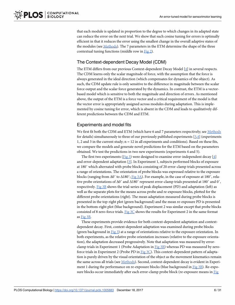
Fig 3. Experiments 1 and 2: Context-dependent adaptation and decay. A. The paradigm for experiments 1 and 2. After an initial exposure
block at 180˚ (yellow background), subjects performed alternating probe blocks presented at one of five orientations between 0˚ and 180˚ (green
background) followed by re-exposure blocks at 180˚ (blue background). B. Experiment 1 in which probe blocks consisted of 20 error-clamp trials.
The left plot shows the composite trial-series for PD (all trials) and Adaptation (error-clamp probe blocks only). Grey shading shows ±SE across
subjects. Each subject experienced the probe blocks in a pseudorandomized order so the trial-series has been rearranged in order of increasing
probe orientation (Δ0˚ to Δ180˚). The right plots show the corresponding measures averaged over the different probe blocks and over subjects
(error-bars show ±SE across subjects). Adaptation is measured from the probe blocks (right top, green background) and re-exposure PD is
measured from the re-exposure blocks (right bottom, blue background). Model fits are shown in all panels for the CDM (blue) and ETM (red).
Experimental data from [4]. C. Experiment 2, plotted as in panel B. In this case, probe blocks consisted of 8 zero-force trials. As in panel B, model
fits are shown in all panels. Experimental data from [3].
https://doi.org/10.1371/journal.pcbi.1005883.g003
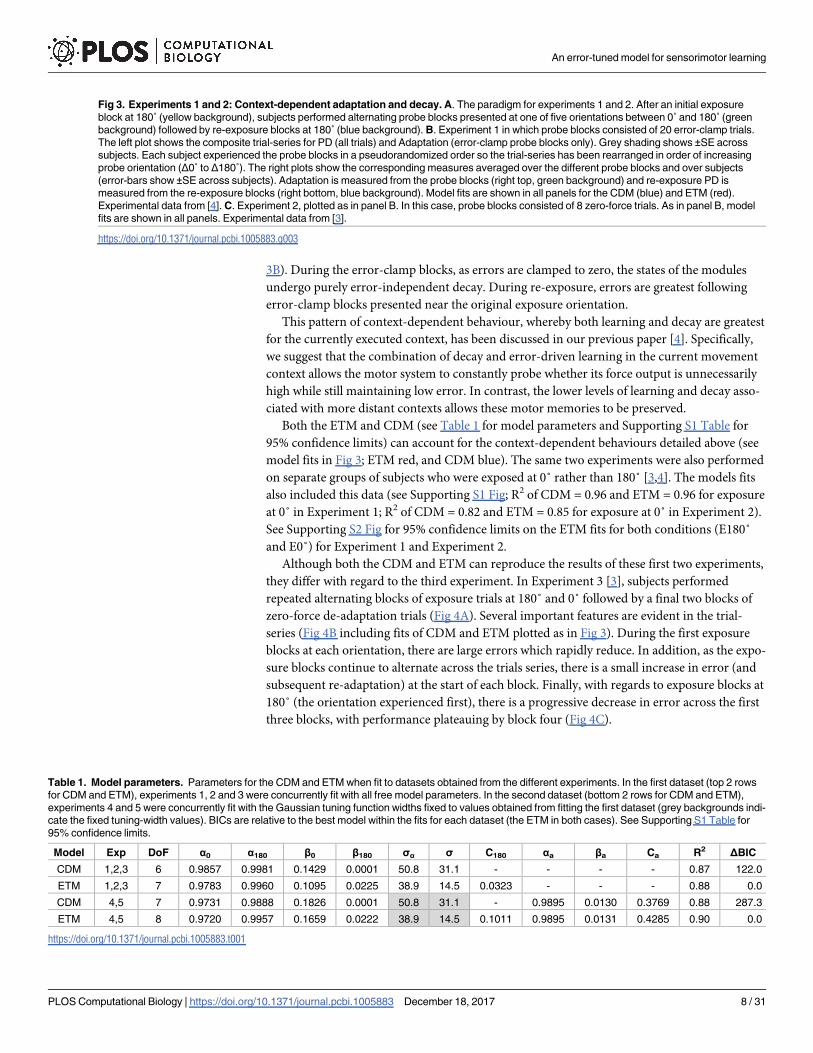
Table 1. Model parameters. Parameters for the CDM and ETM when fit to datasets obtained from the different experiments. In the first dataset (top 2 rows
for CDM and ETM), experiments 1, 2 and 3 were concurrently fit with all free model parameters. In the second dataset (bottom 2 rows for CDM and ETM),
experiments 4 and 5 were concurrently fit with the Gaussian tuning function widths fixed to values obtained from fitting the first dataset (grey backgrounds indi-
cate the fixed tuning-width values). BICs are relative to the best model within the fits for each dataset (the ETM in both cases). See Supporting S1 Table for
95% confidence limits.
Model Exp DoF α0 α180 β0 β180 σα σ C180 αa βa Ca R2 ΔBIC
CDM 1,2,3 6 0.9857 0.9981 0.1429 0.0001 50.8 31.1 - - - - 0.87 122.0
ETM 1,2,3 7 0.9783 0.9960 0.1095 0.0225 38.9 14.5 0.0323 - - - 0.88 0.0
CDM 4,5 7 0.9731 0.9888 0.1826 0.0001 50.8 31.1 - 0.9895 0.0130 0.3769 0.88 287.3
ETM 4,5 8 0.9720 0.9957 0.1659 0.0222 38.9 14.5 0.1011 0.9895 0.0131 0.4285 0.90 0.0
https://doi.org/10.1371/journal.pcbi.1005883.t001
An error-tuned model for sensorimotor learning
PLOS Computational Biology | https://doi.org/10.1371/journal.pcbi.1005883 December 18, 2017 8 / 31
Page 9
In the CDM, the increase in error between the end of one block at a particular orientation
and re-exposure to that same orientation arises purely through error-independent decay.
Importantly, however, as adaptation plateaus by the end of each block, any decay during the
subsequent block will be the same across the experiment. Therefore, the fit of the CDM pre-
dicts that performance for the 180˚ blocks should plateau after the first exposure block (from
the 2nd block; see Fig 4C blue). In contrast, in the ETM, the reduction in performance across
consecutive blocks of the same orientation is not only driven by error-independent decay, but
also by error-dependent interference between the opposing blocks. Because the force gener-
ated by the object for the two orientations (0˚ and 180˚) are in opposite directions (see red vec-
tors in Fig 4A), the kinematic errors will also tend to be in opposite directions. Therefore,
adaptation during an exposure block at 0˚ will be partially driven by a reduction in the
Fig 4. Experiment 3: Opposing dynamics. A. The paradigm consisted of alternating exposure blocks at
180˚ and 0˚ followed by two final blocks of zero-force trials (all blocks consist of 24 trials). B. Trial-series
averaged across subjects (grey shading shows ±SE across subjects). Performance was stable from the 5th
exposure cycle onwards so we omit exposure blocks after this for clarity. The fits of the models are shown in
all panels for the CDM (blue) and ETM (red). C. The PD averaged over each of the first four 180˚ exposure
blocks for the experimental data (error-bars are SE across subjects; p-values are for two-tailed paired t-tests
as indicated) and CDM and ETM fits. Experimental data from [3].
https://doi.org/10.1371/journal.pcbi.1005883.g004
An error-tuned model for sensorimotor learning
PLOS Computational Biology | https://doi.org/10.1371/journal.pcbi.1005883 December 18, 2017 9 / 31
Page 10
adaptive state of the module with a preferred direction of 180˚. This reduction in the adaptive
state of the 180˚ module arises because the error projected onto its preferred direction is nega-
tive (cosine tuning yields -1 in Eq 3). This reduces errors during the 0˚ block, but leads to
increased error during the subsequent 180˚ block, as observed in the trial-series. Moreover,
during the first two exposure blocks of the experiment, the adaptive state of modules corre-
sponding to each orientation is zero. This leads to the large errors observed during these first
two exposure blocks. Importantly, the large errors during the first 0˚ block causes substantial
reduction in the adaptive state (interference) on the 2nd 180˚ block. Over consecutive blocks,
this effect reduces (see experimental data plotted in Fig 4C). The ETM correctly predicts that
the effects of interference should reduce across the first few 180˚ blocks. Therefore, unlike the
CDM (blue plot in Fig 4C), the ETM is able to reproduce the progressive reduction of errors
across 180˚ blocks observed in the data (red plot in Fig 4C).
In addition to these qualitative differences in the predictions of the CDM and ETM in
Experiment 3, a BIC model comparison (see Methods) across all three experiments selects the
ETM over the CDM (ΔBIC = 122.0). See Supporting S2 Fig for 95% confidence limits on the
ETM fits for Experiment 3.
Interference and facilitation
The interference in Experiment 3 arises because the errors experienced on consecutive blocks
are in opposite directions. As a consequence, the modules selective for these errors (180˚ and
0˚) can both contribute to adaptation on a given block (by either increasing or reducing their
adaptive state). However, if the forces generated by the object (and the associated kinematic
errors) on consecutive blocks are orthogonal (see red vectors in Fig 5A for object orientations
at 180˚ and 270˚), the modules selective for these errors (180˚ and 270˚) cannot jointly con-
tribute to adaptation. In the ETM, this arises through the cosine tuning for error. Specifically,
there should be no change in the adaptive state of the module with a preferred direction
orthogonal to the current error. This predicts that the interference patterns observed for
opposing dynamics in Experiment 3 will not occur for orthogonal dynamics.
In addition, the ETM makes a prediction with regards to de-adaptation on zero-force
blocks. On a zero-force block, the errors (after-effects) will be in the opposite direction to
those on an exposure block. Therefore, modules with the preferred direction associated with
the de-adaptation errors will reduce their adaptive state (that is, they should de-adapt). Criti-
cally, however, the ETM predicts that modules with the opposite preferred direction will
increase their adaptive state (because this also contributes to decrease de-adaptation errors).
Therefore, zero-force trials at 0˚ should lead to facilitation (an increase) of adaptation for the
180˚ module. In contrast, zero-force trials at 270˚ should not facilitate adaptation of the 180˚
module, as the errors in this case are orthogonal.
We test the predictions of interference and facilitation in Experiment 4, in which subjects
(n = 12) performed four conditions in a randomized order (Fig 5A). In all conditions, the ori-
entation of the object alternated across successive blocks (as in Experiment 3). All odd-num-
bered blocks were at 180˚ and all even-numbered blocks were either opposing (0˚) or
orthogonal (270˚ as shown in Fig 5A). To examine interference, the first five blocks were expo-
sure blocks and we compared the change in performance between the 2nd and 3rd exposure
blocks at 180˚ (Fig 5A; purple comparison). To examine facilitation, we compared perfor-
mance on the final 180˚ zero-force block when it was preceded by either an exposure block or
a zero-force block (Fig 5A; green comparison). Subjects thus performed four conditions with
two factors: opposing versus orthogonal dynamics and exposure (E6) versus zero-force (Z6)
trials on the 6th block (Fig 5A).
An error-tuned model for sensorimotor learning
PLOS Computational Biology | https://doi.org/10.1371/journal.pcbi.1005883 December 18, 2017 10 / 31
Page 11
Fig 5. Experiment 4: Opposing versus orthogonal dynamics. A. The paradigm consisted of the first five blocks alternating between exposure at 180˚
and exposure at either 0˚ or 270˚ (opposing or orthogonal conditions; here shown as 270˚). Interference was assessed by comparing PD on the 3rd and 5th
block (purple comparison). The sixth block was either exposure (E6) or zero-force (Z6). Facilitation was assessed by comparing PD on the 7th block (Z180˚)
between E6 and Z6 conditions (dark green comparison). B. The trial-series for the four conditions (grey shading shows ±SE across subjects). Rows are
An error-tuned model for sensorimotor learning
PLOS Computational Biology | https://doi.org/10.1371/journal.pcbi.1005883 December 18, 2017 11 / 31
Page 12
The full trial-series for the four conditions and fits for the two models are shown in Fig 5B
(see Table 1 for model parameters and Supporting S1 Table for 95% confidence limits). The
results show significant interference (2nd versus 3rd exposure at 180˚) for the opposing but
not orthogonal dynamics (see purple comparisons in Fig 5B and black bar plot in Fig 5C). The
results also showed significant facilitation for the 180˚ zero-force block when this was preceded
by a zero-force block at 0˚ (opposing) compared to an exposure block at 0˚ (see dark green
comparisons in Fig 5B and black bar plot in Fig 5D). Note that because facilitation is measured
on zero-force trials, it is also manifest as an increase in PD. As predicted by the ETM, no facili-
tation was seen for the orthogonal condition. Analysis of the same measures for the fits of the
model shows that the CDM predicts neither interference nor facilitation (blue plots in Fig 5C
and 5D). In contrast, the ETM predicts both these effects observed in the data (red plots in Fig
5C and 5D). A BIC model comparison across the four conditions in Experiment 4 also selects
the ETM over the CDM (ΔBIC = 115.2). See Supporting S3 Fig for 95% confidence limits on
the ETM fits for Experiment 4.
Visually ambiguous object
The two fundamental components of the ETM that affect adaptation are the contextual tuning
functions (Fig 2A and 2B, blue curves, middle column) and the cosine tuning for kinematic
error (Fig 2B bottom left). The contextual tuning functions determine how the visual orienta-
tion of an object influence both the motor output and the changes in the adaptive state (error-
independent decay and error-dependent adaptation). However, the cosine tuning for error is
independent of the visual orientation of the object. Therefore, the ETM predicts that when
visual information about object orientation is absent or ambiguous, kinematic errors alone are
sufficient to drive adaptation of modules with the appropriate preferred directions.
In Experiment 5, we examine adaptation in the absence of contextual information by pre-
senting subjects with a visually ambiguous object (Fig 1B bottom inset; Fig 6A). Subjects
(n = 12) performed blocks of exposure trials at 180˚ which alternated with probe blocks of
error-clamp trials with orientations of 0˚ and 180˚. Critically, during the exposure blocks, the
normal object dynamics were simulated (exposure at 180˚) and the visual appearance of the
object was ambiguous with regards to its visual orientation (Fig 1B bottom inset; Fig 6A). In
this case, when the contextual information normally provided by vision is ambiguous, the con-
text-dependent tuning functions take on constant values across orientations (see Methods).
Cosine tuning in the ETM predicts that during exposure to a visually ambiguous object, the
kinematic errors experienced by subjects should still selectively adapt modules with the pre-
ferred direction appropriate for the dynamics. To test this, the normal visual orientation of the
object (and the associated contextual tuning of the output) is restored during probe blocks.
The cosine tuning for errors in the ETM predicts that adaptation measured during these probe
blocks should be largest for 180˚ compared to 0˚. Importantly, because the visual probe blocks
consist of error-clamp trials, subjects do not experience the dynamics. Rather, the probe blocks
allow us to probe what modules have adapted to the visually ambiguous dynamics.
The experimental trial-series and model fits (see Table 1 for model parameters and Sup-
porting S1 Table for 95% confidence limits) are shown in Fig 6B (left plot). The results show
that adaption is greatest for the probes at 180˚ compared to 0˚ (black bars for probe adaptation
opposing versus orthogonal dynamics and columns are E6 (exposure trials on 6th block) or Z6 (zero-force trials on 6th block). The model fits are shown in all
panels for the CDM (blue) and ETM (red). Purple and dark green arrows test for interference and facilitation, respectively. C. Interference for the opposing
and orthogonal conditions for the experimental data (black; error-bars show SE across subjects; p-values are for two-tailed paired t-tests) and the two
models (CDM in blue; ETM in red). D. Facilitation, plotted as in panel C.
https://doi.org/10.1371/journal.pcbi.1005883.g005
An error-tuned model for sensorimotor learning
PLOS Computational Biology | https://doi.org/10.1371/journal.pcbi.1005883 December 18, 2017 12 / 31
Page 13
An error-tuned model for sensorimotor learning
PLOS Computational Biology | https://doi.org/10.1371/journal.pcbi.1005883 December 18, 2017 13 / 31
Page 14
in Fig 6B, right top plot, green background), in agreement with predictions of the ETM (red
bars in the same plot). In contrast, the CDM predicts that exposure to visually ambiguous
dynamics should result in the same adaptation across all modules (blue bars in the same plot).
On re-exposure to the ambiguous object at 180˚, PD was greatest after probe blocks at 180˚
compared to 0˚ (black bars for re-exposure PD in Fig 6B, right bottom, blue background).
This arises through context-dependent decay and is also predicted by the ETM (red bars in the
same plot). Specifically, during error-clamp probe blocks, the normal visual appearance of the
object was restored. The model predicts that during such error-clamp trials, context-depen-
dent decay should occur. Thus, if the appropriate modules have adapted to the visually ambig-
uous dynamics, context-dependent decay during probe trials should also be greatest when the
visual context matches those dynamics. This leads to the difference in PD values between the 2
probe contexts in the subsequent re-exposure (re-exposure plots in Fig 6B).
A separate group of subjects (n = 12) were also exposed to the ambiguous object at 0˚ (Fig
6C; Results plotted as for 180˚ exposure in Fig 6B). In this case, adaptation and re-exposure
errors were greatest for the 0˚ probes compared to 180˚, as predicted by the ETM (see bar
plots on the right of Fig 6C). In addition, a BIC model comparison across both the 180˚ and 0˚
groups selected the ETM over the CDM (ΔBIC = 295.3). See Supporting S3 Fig for 95% confi-
dence limits on the ETM fits for Experiment 5.
Object lifting study
A recent study of object lifting is particularly relevant for the ETM model [23]. In this study,
subjects were presented with a U-shaped object that could be lifted by a handle on either the
left (L) or right (R) side (Fig 7A). The task required subjects to lift the object from a table while
minimising the tilt of the object. To do this, subjects had to apply compensatory torques on
the handle as they lifted the object (a CCW torque for the left handle and a CW torque for the
right handle). The visual location of the centre of mass relative to the grasp points is similar to
the visual orientation of the object in our task. In the lifting study, subjects performed four
consecutive blocks (8 trials each) with the context (lifting left or lifting right) alternating across
blocks (Context 1 and Context 2). Task performance was measured as the peak tilt angle of the
object during lifting and also the peak compensatory torque prior to object lift off [23].
When lifting the object for the first time, subjects used visual geometric cues about the
object (the mass, centre of mass and location of the grasp point). This allowed them to lift the
object with a small tilt angle and a torque close to that required for full compensation (first
trial, Fig 7B). However, despite almost perfect performance by the end of the first block (Con-
text 1), subjects showed significant errors when switching to the opposite handle (Context 2).
These larger errors during the second block (for Context 2) suggest that interference is occur-
ring (as observed in our experiments 3 and 4). Here, we show that the ETM can also account
for this interference observed when lifting real-world objects.
Fig 6. Experiment 5: Visually ambiguous object. A. The paradigm consisted of initial exposure to a visually ambiguous object
with dynamics at 180˚ (yellow background), after which subjects perform alternating probe blocks (20 error-clamp trials) at one of
two orientations (0˚ or 180˚; green background) followed by re-exposure to the visually ambiguous object with dynamics at 180˚. B.
The right plot shows the composite trial-series for PD (all trials) and Adaptation (error-clamp probe blocks only). Grey shading
shows ±SE across subjects. Each subject experienced the probe blocks in a pseudorandomized order. The trial-series has been
rearranged in order of probe orientation (Δ0˚ and Δ180˚). The right plots show the corresponding measures averaged over the
different probe blocks and over subjects (error-bars show SE across subjects; p-values are for two-tailed paired t-tests as
indicated). Adaptation is taken from the probe blocks (right top, green background) and re-exposure PD is taken from the re-
exposure blocks (right bottom, blue background). The model fits are shown in all panels for the CDM (blue) and ETM (red). C. A
second group of subjects was exposed to the visually ambiguous object with dynamics at 0˚. Results are plotted as in panel B.
https://doi.org/10.1371/journal.pcbi.1005883.g006
An error-tuned model for sensorimotor learning
PLOS Computational Biology | https://doi.org/10.1371/journal.pcbi.1005883 December 18, 2017 14 / 31
Page 15
We can consider the object lifting experiment within the same framework as the ETM
model (see Methods). In this case, each module can generate a torque around a single fixed
preferred oriented axis. The preferred torque axes across modules uniformly covers all orienta-
tions in the horizontal plane (corresponding to θi in the ETM). The context is the orientation
of the centre of mass relative to the handle. As the original study only used two orientations
(two grasp handles), we fit a simplified version of the ETM with only two modules (θi 2
{0˚,180˚}) which correspond to producing CCW and CW torques for the left and right han-
dles. In addition, we assumed that the initial adaptive state of both modules (x˚) was non-zero
and we include this as a fit parameter. This initial state represents existing knowledge of the
dynamics of lifting objects, which may be based on visual cues.
The ETM successfully reproduces the experimental data for both absolute peak tilt angle
and the compensating torque (Fig 7B, R2 = 0.99 across both measures). In particular, it repro-
duces the interference observed when switching from the first block (Context 1) to the second
Fig 7. Object lifting experiment. A. The lifting paradigm used in [23]. Participants lifted a U-shaped object by alternating between the right-hand and
left-hand grasp points in four blocks. B. The peak roll angle (tilt) of the object (top panel), as well as the compensation torque (bottom panel). Perfect
compensation required ±550 N.mm depending on the context. Data is plotted in black and the fits for the ETM and CDM are plotted in red and blue,
respectively. The best-fit parameters for the models (see Methods for details) are: α0 = 0.87, β0 = 0.74, β180 = 0.17, c180 = 0.0, x˚ = 0.66, and k = 15.68
for the ETM, and α0 = 0.92, β0 = 0.79, β180 = 0.00, c180 = 0.49, x˚ = 1.00 and k = 15.68 for the CDM.
https://doi.org/10.1371/journal.pcbi.1005883.g007
An error-tuned model for sensorimotor learning
PLOS Computational Biology | https://doi.org/10.1371/journal.pcbi.1005883 December 18, 2017 15 / 31
Page 16
block (Context 2). It also reproduces the interference observed during re-exposure in the third
and fourth blocks. In contrast, because the CDM does not model interference, it underesti-
mates error during the third and fourth blocks (Fig 7B, R2 = 0.97).
Discussion
We have developed a novel state-space model, the error-tuned model (ETM), which is based
on a modular architecture. Each module produces force in a particular direction (its preferred
direction) and can contribute to the net motor output in the two-dimensional task space.
Modules do not change their preferred direction, but rather change their adaptive state, which
determines their contribution to the net motor output. Critically, adaptation in the model
(changes in the adaptive state across modules) is influenced by two processes. First, top-down
contextual information (the visual orientation of the object) selectively weights the contribu-
tion of modules to the motor output. Contextual information also determines the degree to
which errors update the adaptive states of each module. Second, bottom-up information pro-
vided by the magnitude and direction of kinematic errors also influence the adaptive states
across modules. Specifically, each module is tuned to a particular error (determined by its pre-
ferred direction), and can change its adaptive state in proportion to its ability to correct the
error. This selectivity for errors is implemented by cosine tuning for error direction.
The presence of error-tuned modules in the ETM makes two predictions which we confirm
experimentally. First, cosine tuning predicts that dynamics which generate opposite kinematic
errors will interfere. This arises because adapting to dynamics which cause kinematic errors in
one direction will be partially achieved by reducing the activity (cosine tuning of -1) of mod-
ules appropriate for the opposite direction. In contrast, dynamics that generate orthogonal
errors should show little interference. This arises because the cosine tuning for orthogonal
errors (cosine tuning of 0) does not change the activity of the associated modules. We confirm
these predictions, showing that interference is eliminated for orthogonal dynamics (Fig 5).
Second, because errors can select the appropriate modules for update, the model predicts the
selective adaptation of appropriate modules even in the absence of visual context. Using a visu-
ally ambiguous object, we show that the appropriate modules can adapt based on kinematic
error in the absence of contextual information (see Fig 6). Together with the ability to account
for previous data, these new results support a modular error-tuned model of motor learning.
Evidence for modularity in sensorimotor control has come from a variety of studies [1–6].
However, the details of module selection remain poorly understood. For example, studies of
motor synergies have largely focused on extracting the patterns of muscle activity which
underlie each synergy whereas the mechanisms by which different synergies are selected for a
particular movement have received less attention [14–19]. Similarly, studies of motor learning
have commonly focused on the acquisition of new internal models whereas less is known
about the mechanisms by which these newly acquired models are selected from existing mod-
els [1,7–9]. As a result, the majority of computational models which include module selection
rely on a single simplified mechanism [10,29]. In most cases, these mechanisms do not distin-
guish between kinematic factors (such as different movement directions) and contextual fac-
tors (such as the different states of a manipulated object). Moreover, the role of movement
error in module selection, although suggested by theoretical studies [8], has received little
experimental attention. In contrast, the ETM presented in the current study combines two
mechanisms for module selection. As well as contextual information, which is the only mecha-
nism considered by most current models, the ETM includes an error-based selection mecha-
nism (cosine tuning for error).
An error-tuned model for sensorimotor learning
PLOS Computational Biology | https://doi.org/10.1371/journal.pcbi.1005883 December 18, 2017 16 / 31
Page 17
The concept of motor primitives has been previously used in sensorimotor learning models
mainly to study adaptation of reaching movements under state-dependent force-fields [12]. In
these studies, primitives were defined in position and velocity space and were fit to experimen-
tal data to study biases seen when learning different types of force fields. A recent study [5]
proposed a model based on a different form of motor primitives to explain how prospective
(i.e. predicted) errors drive sensorimotor learning. In this model, primitives are defined in
error space and are activated based on the size and sign of the prospective errors through a
Gaussian function. The proposed model could explain several features of motor learning.
However, the domain of predictions was limited to tasks with a one-dimensional error space
and under a single context (for example, reaching in a single direction). In contrast, the primi-
tives in the ETM represent force production in a two-dimensional space and they directly con-
tribute to the motor output. In addition, the ETM primitives are activated jointly by two
separate mechanisms; one based on the visual context of the environment, and the other based
on the two-dimensional kinematic error.
The ETM and the previous models [3,4] that we have fit to our object manipulation task are
all single-rate state-space models. These models have a single fast rate of adaptation which we
assume is associated with a single adaptation process. Previously, we have speculated [3,4] that
this fast single-rate adaptation process may be engaged when familiar dynamics are encoun-
tered (for example, the dynamics of everyday objects). In contrast, dual-rate state-space models
have been applied to tasks in which the dynamics are novel and unfamiliar [26]. Dual-rate
models assume that adaptation is mediated by distinct processes with different rates of adapta-
tion. For example, these processes appear to map to different (explicit versus implicit) learning
strategies [31] and appear to be independently affected by aging [32]. The relationship between
the dual-rate adaptation processes examined in these previous studies and the single-rate pro-
cess which mediates adaptation in the ETM are currently unknown. Further theoretical and
experimental work would be required to elucidate this matter.
Interference has been observed across a range of motor tasks [33–37]. The demonstration
of interference during object lifting is of particular relevance to the current study [23]. In our
current study, the task required subjects to rotate an object while preventing it from translat-
ing, whereas in the object lifting task, subjects are required to translate (lift) an object while
preventing it from rotating (tilting) by applying an appropriate torque [23]. In both cases,
visual information about the context of the object as well as the direction and magnitude of
kinematic errors can potentially contribute to adaptation across successive trials. In the ETM,
these sources of information are combined in order to update the adaptive states of an array of
modules which have different preferred directions of force output. Interference arises as a nat-
ural consequence of this modular architecture. Specifically, interference arises due to the inter-
action between errors and module output, but only when these are in opposite directions.
Therefore, the ETM can model interference in the object rotation task and in the previous
object lifting task (Fig 7). Importantly, in the current study, the ETM also correctly predicted
that the interference observed for opposing dynamics should be reduced for orthogonal
dynamics (Fig 5).
As discussed above, in the ETM, interference is a natural consequence of the interaction
between modules with opposite preferred directions. An alternative model has previously been
proposed to explain interference during object lifting [38]. In this model, interference between
the modules producing CW and CCW torques does not arise due to the interaction between
modules with opposite preferred directions (as it does in the ETM). This is because the terms
which mediate this interaction have been specifically set to zero in the model. Rather, interfer-
ence in this previous model is captured by a bias term which is added to the motor output.
Our simulations show that if modules with opposite preferred directions are allowed to
An error-tuned model for sensorimotor learning
PLOS Computational Biology | https://doi.org/10.1371/journal.pcbi.1005883 December 18, 2017 17 / 31
Page 18
interact (with non-zero interaction terms), this bias term becomes unnecessary to reproduce
interference. Moreover, it is unclear whether the bias term could generalize to account for our
results in two dimensions.
A number of studies have examined the role of contextual information in engaging sensori-
motor modules prior to movement [21,39]. For example, studies have shown that contextual
cues can reduce the interference that normally occurs between two opposing velocity-depen-
dent force-fields [39–43]. These studies show that when contextual information is provided
which distinguishes between the two fields, subjects can adapt their feed-forward motor com-
mands to the opposing dynamics. These results provide evidence that contextual information
is used to select between separate internal models of task dynamics prior to a movement. In
contrast, the role of movement errors in engaging and updating sensorimotor modules is less
well understood. Importantly for the modular framework of sensorimotor control, evidence
that movement errors can selectively engage and modify the output of specific sensorimotor
modules is also lacking. In the current study, we provide evidence that modules are indeed
tuned to movement errors so as to respond appropriately depending on their ability to correct
an error. In neurophysiological studies, similar tuning for the direction of movement errors
has also been found at the level of single neurons [e.g. 44, 45].
In the ETM, the error-based selection of modules is mediated by a cosine tuning function.
For a particular error, cosine tuning determines the extent to which each module should
change its activity so as to reduce the error progressively in the following trials. In previous
studies, cosine tuning functions have been used effectively in the analysis of various features of
the motor system, from tuning curve characteristics of motor cortical cells [46] to determining
the contribution of muscle activity in force generation [47]. It has also been shown that cosine
tuning can be an optimal solution in some cases, such as minimizing the net effect of neuro-
muscular noise in force production [48]. Here, we show mathematically that cosine tuning of
modules to the direction of error in the ETM leads to an optimal selection process akin to a
minimum intervention principle (see Methods). We demonstrate that for a particular error,
cosine tuning will reduce the error with the minimum possible change in the activity across
the modules.
Although the ETM is a high-level computational model, it is possible to speculate about its
neural implementation in the brain. For example, there are three critical components of the
ETM and these may be associated with known neural mechanisms. First, modules in the ETM
have a preferred direction of force output and cells in primary motor cortex have also been
found to have a preferred direction of action [46]. Second, contextual information about the
visual orientation of the object mediates the top-down selection of modules in the ETM and
the parietal cortex is thought to specifically encode object orientation when such information
is required by the motor system [49]. Thirdly, modules in the ETM are tuned for the direction
of kinematic errors and cells selective to error direction have been found in the cerebellum
[50]. How these and other neural mechanisms are combined for the control of movement is an
important topic for research.
The results of the current study suggest that sensorimotor modules are tuned to detect spe-
cific errors, changing their contribution to the motor output only if such a change is appropri-
ate for reducing that particular error. We have demonstrated that such a process can account
for adaptation seen when manipulating objects and also in a previous study of lifting objects.
These were specific tasks which operated in a two-dimensional space. However, modular
architectures have been implicated in a variety of different forms and across a variety of differ-
ent tasks. The selective tuning of modules to particular errors may thus be a general feature of
motor learning. In this view, across the array of possible modules which may be involved in a
particular task, a central mechanism for motor learning is the ability of each module to detect
An error-tuned model for sensorimotor learning
PLOS Computational Biology | https://doi.org/10.1371/journal.pcbi.1005883 December 18, 2017 18 / 31
Page 19
those errors which are relevant to its output. Such error-tuning may be a general principle of
sensorimotor control.
Materials and methods
Ethics statement
The study was approved by the Cambridge Psychology Research Ethics Committee. The sub-
jects (a total of 96 university students) gave written informed consent before participating and
were naïve to the purpose of the study.
The object manipulation task
The object manipulation task has been previously described [3]. Briefly, subjects were seated at
a virtual reality system and grasped the handle of a planar robotic manipulandum (the Wrist-
BOT) with their right hand (Fig 1A). The WristBOT [30] simulated the dynamics (forces and
torques) of a hammer-like object which consisted of a mass on the end of a rigid rod (Fig 1B).
Subjects grasped the object by a handle at the base of the rod (the grasp point in Fig 1B).
The virtual reality display system provided visual feedback associated with the object and
the task (Fig 1B). The visual object consisted of a circular handle (radius 0.5 cm) attached by
an 8 cm rod (width 0.2 cm) to a 4 cm square mass. The task involved rotating the object 40˚
between two visually presented targets (0.6 x 2.5 cm oriented rectangles). Subjects made alter-
nating clockwise (CW) and counter-clockwise (CCW) rotations across trials (Fig 1B) and were
asked to maintain the handle as still as possible within a central home region (1 cm radius).
The position and orientation of the object tracked the position and orientation of the Wrist-
BOT handle. The angular midpoint between the two targets defined the orientation of the
object and this could vary across trials in the experiments (the targets were thus ±20˚ relative
to the presentation orientation).
The object dynamics
The dynamics of the object were simulated as a point mass (1% of the subject’s body mass) at
the end of the rigid rod (Fig 1B). Rotating the object generated forces and torques at the handle
which were simulated by the manipulandum. The torque was associated with the moment of
inertia of the object and the force was associated with the circular motion of the mass (τ and F,
respectively in Fig 1B). Critically, the force caused the handle to displace unless subjects pro-
duced a compensatory force in the opposite direction (for full details about the object dynam-
ics see [3]). Briefly, the force generated by rotating the object is dominated by the tangential
acceleration of the mass and is approximately perpendicular to the rod. The direction of the
force depends on the orientation of the object whereas its magnitude depends on the mass and
the length of the rod. We have previously shown that subjects produce compensatory forces in
the direction which is appropriate for the visual orientation of the object from the very first
trial, even before they have experienced the dynamics in the task [24]. This is evidence that
subjects have pre-existing knowledge (an internal model) of the dynamics of such objects.
Moreover, subjects rapidly adapt the magnitude of these forces in order to minimise displace-
ment of the handle [3].
A trial began with the handle stationary within the home region and the object aligned with
the start target for that trial. The movement was cued by a tone and the appearance of the end
target (40˚ from the start target). A successful trial ended when the subject had rotated the
object to reach the end target. The end target then became the start target for the next trial
An error-tuned model for sensorimotor learning
PLOS Computational Biology | https://doi.org/10.1371/journal.pcbi.1005883 December 18, 2017 19 / 31
Page 20
(inset of Fig 1B). Subjects were required to make the movement within 400 ms, were warned if
they took longer and had to repeat the trial if the movement exceeded 500 ms.
Trial types
Subjects experienced the torque associated with rotating the object on all trials. However, the
forces generated by the manipulandum could vary according to three different trial types. On
exposure trials, subjects experienced the forces associated with rotating the object (that is, they
experienced the full dynamics of the object). On error-clamp trials, the manipulandum simu-
lated a stiff two-dimensional spring centred on the handle position at the start of the trial (the
spring constant was 40 N/cm). Error-clamp trials effectively eliminate kinematic errors [51]
and prevent error-driven adaptation. Error-clamp trials also allow the compensatory forces
produced by subjects to be measured. Finally, on zero-force trials, the manipulandum did not
produce any forces and the handle was free to move. Importantly, any forces produced by sub-
jects on zero-force trials will cause the handle to displace.
Experiments
Five experiments were performed. A partial analysis of experiments 1, 2 and 3 has been previ-
ously published and we include brief methods here (full details in [3,4,24]). All experiments
began with a familiarization phase which consisted of repeated blocks of 12 zero-force trials.
The blocks were presented at all orientations which subjects would experience during the par-
ticular experiment. Zero-force familiarization blocks for each orientation were repeated twice
and presented in a pseudorandom order. This ensured that the force output produced by sub-
jects prior to the experiment was low. Rest breaks (45 s) were given every 3–5 minutes in all
experiments.
In Experiment 1, subjects (n = 12) first performed a block of 46 exposure trials at a single
exposure orientation (E180˚; Fig 3A and 3B). They were then presented with repeating probe
blocks consisting of 20 error-clamp trials at one of five possible probe orientations (Pθ˚ relative
to the exposure orientation, Pθ = {0˚, 22.5˚, 45˚, 90˚, 180˚}). Each probe block was followed by
a re-exposure block consisting 18 exposure trials with the object at the original exposure orien-
tation (E180˚). Each of the 5 probe block orientations was repeated 3 times in a pseudorandom
order (total of 15 probe blocks). A second group (n = 12) performed the identical experiment
except that they were exposed at 0˚ (E0˚).
Experiment 2 was identical to Experiment 1 except that in this case the probe blocks con-
sisted of 8 zero-force (de-adaptation) trials (Fig 3A). Again, separate groups of subjects (n = 12
in each group) were exposed to the object at 180˚ (E180˚; Fig 3A and 3C) and 0˚ (E0˚).
In Experiment 3, subjects (n = 12) performed 20 alternating blocks of 24 trials at 180˚ and
0˚ (10 blocks of each). The first 18 blocks were exposure trials (E180˚ and E0˚ in Fig 4A) and
the last two block were zero-force trials (Z180˚ and Z0˚ in Fig 4A).
In Experiment 4, subjects (n = 12) performed four conditions in a randomized order (Fig
5A). In all conditions, the orientation of the object alternated across successive blocks (as in
Experiment 3). All odd-numbered blocks were at 180˚ and all even-numbered blocks were
either 0˚ (opposing dynamics condition; as in Experiment 3) or 270˚ (orthogonal dynamics
condition as shown in Fig 5A). The first five blocks of the four conditions were always expo-
sure blocks and the last two blocks were always zero-force blocks (Fig 5A). In the E6 condition,
an additional exposure block at either 0˚ or 270˚ was performed before the final zero-force
blocks. The four conditions thus comprised a combination of two factors: opposing versus
orthogonal dynamics and exposure (E6) versus zero-force (Z6) trials on the 6th block.
An error-tuned model for sensorimotor learning
PLOS Computational Biology | https://doi.org/10.1371/journal.pcbi.1005883 December 18, 2017 20 / 31
Page 21
In Experiment 5, subjects (n = 12) performed a block of 46 exposure trials with dynamics
corresponding to an object at 180˚. However, the rod and mass of the object were not dis-
played making the orientation visually ambiguous. To guide the appropriate rotations of the
object, the object was displayed as a disc with small bars at 0˚ and 180˚ (see bottom inset of Fig
1B and exposure object in Fig 6A). As in the other experiments, these bars had to be aligned
with the angular targets presented during the task. Importantly, the visual display of the
ambiguous object still tracked the rotation and translation of the WristBOT handle. After the
initial exposure block, subjects performed probe blocks of 20 error-clamp trials which alternat-
ing with re-exposure blocks of 18 exposure trials. Probe blocks were presented at one of two
probe orientations (P0˚ and P180˚; Fig 6A) and importantly, the normal visual object was dis-
played during the probes. During the re-exposure blocks, the visually ambiguous object was
re-displayed. Each probe orientation was repeated 3 times in a pseudorandom order. A second
group of subjects (n = 12) performed the identical experiment except that they were exposed
to the visually ambiguous object with the dynamics at 0˚ (E0˚; Fig 6C).
Analysis
On zero-force and exposure trials, the peak displacement (PD) of the handle was measured,
relative to its position at the start of the trial. Peak displacement is a measure of error, because
the task required subjects to keep the handle as still as possible as they rotate the object. A PD
of zero would thus indicate perfect performance. On error-clamp trials, the peak force pro-
duced by subjects was measured as the restoring force of the 2D simulated spring. Peak force is
a measure of the subject’s adaptation to the object dynamics. Adaptation was calculated as the
ratio of the peak force divided by the peak force that would fully compensate for the dynamics
of the object on that trial. For example, at 0.5 adaptation the peak force produced by a subject
during the rotation would be half the force generated by the object.
For experiments which included repeated blocks of probes trials (experiments 1, 2 and 5),
we first averaged trial data for each subject across the repeats for each probe orientation and
then averaged across subjects. We then created a composite trial-series consisting of the initial
exposure trials (averaged across subjects), followed by the average probe blocks in order of
increasing relative probe orientation (Δθ). These composite series were used for fitting the
models and for presenting the data. Note that as the adaptive state is very similar at the start of
each probe block, the order of the probe blocks in the composite trial series has minimal effect
on the model parameters.
The Error Tuned Model (ETM)
The Error Tuned Model (ETM) is a state-space model which implements a mixture-of-primi-
tives modular architecture. Each module (or primitive) can produce force in only a single
direction termed the module’s preferred direction (specified by θi for the ith module). There-
fore, each module can produce positive force in the direction of a 2-dimensional unit vector:
ui ¼cosyi
sinyi
" #
ð4Þ
The m modules cover the range of possible force directions uniformly across 360˚ (in the
two-dimensional task space). Each module is associated with a positive adaptive state (xðnÞi on
the nth trial) which can change over trials. The adaptive state represents the activity of that
module. We represent the ensemble of preferred module directions as Θx = [θ1,. . .,θm]T and
their adaptive states on trial n as xðnÞ ¼ ½xðnÞ1 ; . . . ; xðnÞm �T
(Fig 2A, left panel). On a given trial, the
An error-tuned model for sensorimotor learning
PLOS Computational Biology | https://doi.org/10.1371/journal.pcbi.1005883 December 18, 2017 21 / 31
Page 22
visual orientation of the object can be informative as to the direction of force required to com-
pensate for the dynamics. We define yðnÞv as this force direction based on the visual orientation
of the object and define the vector Δ(n) as the difference between this angle and the preferred
force directions of all the modules: ΔðnÞ ¼ Yx � yðnÞv (with the ith element denoted by D
ðnÞi ).
The net motor output (z(n); Fig 2A, right panel) is a vector sum of force vectors weighted by
both the adaptive states across modules and a contextual tuning function:
zðnÞ ¼Xm
i¼1
CðDðnÞi Þ � xðnÞi � ui ð5Þ
The contextual tuning function, CðDðnÞi Þ, gives greater weights to modules whose preferred
force direction is close to the direction that can compensate for the dynamics of the object,
and progressively less weight as the preferred direction deviates (Fig 2A, middle panel). The
contextual weight is represented as a Gaussian function of DðnÞi , with standard deviation σc,
scaled to have a maximum of 1 (at DðnÞi ¼ 0) and a minimum of c180 (at D
ðnÞi ¼ �180). There-
fore, the net output is affected by both the adaptive states across modules as well as contextual
information provided by vision of the object.
The adaptive states of the modules change across trials based on both error-independent
decay and error-dependent adaptation:
xðnþ1Þ ¼ αðΔðnÞÞ � xðnÞ þ βðΔðnÞÞ � cosðYx � yðnÞe Þ � e
ðnÞ ð6Þ
where� denotes element-wise vector multiplication. The first term specifies the error-inde-
pendent decay (Fig 2B, top row) and is mediated by a context-dependent retention function
α(Δ(n)), whose elements determine the extent to which the adaptive state of each module is
retained on the next trial (Fig 2B, top row, middle panel). This decay function is represented as
a Gaussian function of Δ(n) with standard deviation σα, scaled to have values between α0 and
α180, at DðnÞi ¼ 0� and D
ðnÞi ¼ �180�, respectively.
The second term specifies the error-dependent adaptation (Fig 2B, bottom row) which
updates the states based on the magnitude of the error (e(n)). The state update for each module
in response to this error is dependent on two factors. First, the error is weighted by a visual
context-dependent learning rate β(Δ(n)) which is a Gaussian function of DðnÞi with standard
deviation σβ, scaled to have a value of β0 and β180, at DðnÞi ¼ 0� and D
ðnÞi ¼ �180�, respectively
(Fig 2B, bottom row, middle panel). Therefore, in general, the module which should be able to
contribute most to reduce error (based on the visual orientation of the object) is updated the
most. The second factor modulating adaptation depends on the direction of the kinematic
error. In the model, each module can only reduce errors along its preferred force direction by
increasing or decreasing its adaptive state. Therefore, the adaptive state of each module is
changed in proportion to the component of error projected onto its preferred force direction.
This projection is calculated by multiplying the magnitude of the error (e(n)) by the cosine of
the angular difference between the error direction (yðnÞe ) and the preferred force direction for
each module (Fig 2B, bottom row, left panel).
Without loss of generality, we define the force generated by the object on exposure trials to
have unit magnitude. The kinematic error is determined by the discrepancy between the force
output of the model (which represents the force produced by the subject) and the force pro-
duced by the object. The error magnitude is also modulated by a compliance-dependent func-
tion. The error also depends on whether the trial is an exposure trial (p = 1) or a zero-force
An error-tuned model for sensorimotor learning
PLOS Computational Biology | https://doi.org/10.1371/journal.pcbi.1005883 December 18, 2017 22 / 31
Page 23
trial (p = 0):
eðnÞ ¼ fyðnÞv ;pðnÞ � ðp
ðnÞcosyðnÞv
sinyðnÞv
2
4
3
5 � zðnÞÞ ð7Þ
Here, fyðnÞv ;pðnÞ linearly maps state errors in the model to the magnitude of kinematic errors
and is specified separately for each object orientation and trial type (zero-force and exposure).
The error vector magnitude (e(n)) and angle (yðnÞe ) are then used to update the adaptive states
across modules (Eq 6). On error-clamp trials e(n) = 0.
Model fitting
The free parameters of the ETM model include: c180, σc, β0, β180, σβ, α0, α180, and σα. In the fits
and simulations, we used m = 16 modules. We set the standard deviations for the Gaussian
functions tuning functions CðDðnÞi Þ and β(Δ(n)) to be equal (σc = σβ = σ), both to reduce the
degrees of freedom in the model and because the experimental paradigms were not designed
to constrain each of these parameters separately. The number of free parameters in the ETM
was thus 7. The compliance-dependent error function (fyðnÞv ;pðnÞ) has been previously estimated
for this task and we used these values [3].
There are two measures from the experimental trial-series. On zero-force and exposure tri-
als we measure peak displacement whereas on error-clamp trials we measure adaptation. To
use all the trials to fit the model we need to represent them in the same units. Therefore, for
error-clamp trials we converted both the adaption measured on that trial, as well as the motor
output predicted by the model, to the equivalent kinematic error using Eq 7. For each experi-
ment we averaged the trial data across subjects and then fit by minimizing the mean squared
error between the empirical and predicted kinematic errors.
The 7 parameter ETM was fit simultaneously to the trial-series from experiments 1, 2 and 3.
The trial-series were obtained from 5 different groups of subjects (2 groups for the 2 condi-
tions in Experiment 1, 2 groups for the 2 conditions in Experiment 2, and 1 group for Experi-
ment 3). Experiments 4 and 5 were also fit simultaneously. Because experiments 4 and 5 only
use a limited number of object orientations (no more than three) they were not able to con-
strain the σ and σc parameters of the Gaussian tuning functions. We therefore fixed these
parameters to the values obtained from fitting the first three experiments. In Experiment 5, we
used a visually ambiguous object. On the trials where the visually ambiguous object was pre-
sented, the context-dependent tuning functions CðDðnÞi Þ, α(Δ(n)) and β(Δ(n)), were set to be
constant across all orientations. This required three additional parameters: ca, αa and βa.
To account for differences in the stiffness and other biomechanical properties across the
groups of subjects, we also included parameters that allowed the peak displacement and adap-
tation measures to be related linearly to the model predictions for each subject group. Impor-
tantly, because these additional parameters can only scale model output uniformly within each
group of subjects, they do not qualitatively influence the predictions of the model (which are
always tested within each group).
Modelling object lifting
We also fit the ETM and CDM to results from a previous study [23] in which subjects lifted a physi-
cal object using handles (grasp points) either on the left or right side of the object (Fig 7A). Subjects
were asked to lift the object while minimizing tilt. This required them to generate compensatory tor-
ques which depended on the location of the centre of mass relative to the grasp point.
An error-tuned model for sensorimotor learning
PLOS Computational Biology | https://doi.org/10.1371/journal.pcbi.1005883 December 18, 2017 23 / 31
Page 24
In the case of object lifting, each module in the ETM can generate a torque around a single
fixed preferred oriented axis (with torque direction specified by the right-hand rule). The con-
text is the orientation of the centre of mass relative to the grasp point. In general, the preferred
axes across modules would uniformly cover all orientations in the horizontal plane (corre-
sponding to θi in the ETM). However, as this previous study used only two orientations (two
grasp points), we fit a simplified version of the ETM which has two modules, θi 2 {0˚, 180˚}.
These modules correspond to producing CCW and CW torques for the left and right grasp
points. In this case, the ETM generates torques aimed at minimising object tilt (instead of
forces aimed at minimising object displacement).
The ETM with only two modules reduces the degrees of freedom of the model from 7 to
5 (because with only two orientations in the experiment, the σα and σ parameters for the
contextual tuning functions are not fit). For simplicity, we also set the retention factor for
the non-preferred module (α180) to 1. Because subjects have an initial estimate of the torque
required to lift objects in this task (for example, based on visual cues), we assumed that the
adaptive state of both modules (x˚) was initially non-zero and we also fit this parameter. We
fit absolute error from the model (e(n)) to the absolute peak object tilt from the experiment.
We included an additional fit parameter (k) which scaled the motor output to units of peak
roll. After fitting the model, we performed a linear regression to map the output of the
model (z) to the experimental torque data (see Fig 7B). The same process was repeated for
fitting the CDM.
The Context-Dependent Decay Model (CDM)
For comparison with the ETM, we also include fits of our previous context-dependent decay
model (CDM; [4]). The CDM differs from the ETM in two critical aspects. First, the CDM
describes the motor output and errors as signed scalar values rather and 2D vectors. The scalar
value for motor output in the CDM represents only the magnitude of the force required to
compensate for the object dynamics and in this case is simply the adaptive state of the cur-
rently selected module. The sign of the scalar error indicates whether the motor output on a
given trial is too small (positive errors) or too large (negative errors) to compensate for the
object dynamics on that trial. Second, because errors are signed scalars in the CDM, there is
no tuning for the direction of error. In contrast, in the ETM, tuning for the direction of error
is critical to the model and is implemented by the cosine term in Eq 6. Despite the differences
between the current ETM and previous CDM, the equations for the CDM can be expressed
using similar notation. The scalar motor output in the CDM is:
zðnÞ ¼Xm
i¼1
CðDðnÞi Þ � xðnÞi ð8Þ
where, CðDðnÞi Þ is now a binary selection function that is 1 for module i when DðnÞi ¼ 0, and is 0
otherwise. That is, only the module whose preferred direction matches the orientation of the
object contributes to the motor output. The state-update equation for the CDM is:
xðnþ1Þ ¼ αðΔðnÞÞ � xðnÞ þ βðΔðnÞÞ � eðnÞ ð9Þ
Where, the functions α(Δ(n)) and β(Δ(n)) are the retention and learning-rate functions,
respectively (as defined in the ETM). Finally, the error in the CDM is a signed scalar:
eðnÞ ¼ fyðnÞv ;pðnÞ � ðp
ðnÞ � zðnÞÞ ð10Þ
An error-tuned model for sensorimotor learning
PLOS Computational Biology | https://doi.org/10.1371/journal.pcbi.1005883 December 18, 2017 24 / 31
Page 25
Where, fyðnÞv ;pðnÞ and p(n) is the compliance-dependent error function and the trial-type indi-
cator, respectively (as in Eq 7 for the ETM). The CDM therefore has 6 parameters (the same
parameters as the ETM, excluding c180).
Model comparison
Model selection between the ETM and CDM was performed using the Bayesian Information
Criterion (BIC). The BIC for a particular model combines a ‘‘reward” for the goodness of fit
with a ‘‘penalty” for the number of free parameters:
BIC ¼ N � lnðs2
eÞ þ k � lnðNÞ ð11Þ
where s2e is the variance in the residual errors of the fit, k is the number of free parameters and
N is the number of data points (the number of trials). Taking the difference in BIC values for
two competing models approximates half the log of the Bayes factor [52]. A BIC difference of
greater than 4.6 (a Bayes factor of greater than 10) is considered to provide strong evidence in
favour of the model with the lower BIC value [53].
Bootstrap analysis
Confidence limits for the model fits, model parameters and R2 values were calculated using a
bootstrap analysis [3,26]. Specifically, 10,000 unique samples of 12 subjects were drawn with
replacement from the subject pool for each experiment (n = 12 subjects in all experiments).
The models were fit separately to the mean of each bootstrap sample, as described above. The
95% confidence limits were calculated as the 2.5 and 97.5 percentile values from the distribu-
tions for the model fits, model parameters and R2 values across the 10,000 samples. P-values
for the BIC model selection were calculated as the proportion of samples with BIC values in
favor of the selected model.
The 95% confidence limits for the model fits across the 5 experiments are shown as shaded
error-bars in the Supporting S2 and S3 Figs. The 95% confidence limits for model parameters
and R2 values, and the p-values for BIC model selection are presented in Supporting S1 Table.
Optimality of cosine error tuning
In addition to model fitting and simulations, we also show that cosine tuning for errors in the
state-update function (adaptation) is optimal in reducing the error with the minimal change in
the adaptive states of the modules (akin to the minimum intervention principle). For simplic-
ity, we consider the update rule in the absence of both contextual information and error-inde-
pendent decay.
Consider m modules with adaptive states x = [x1,. . .,xm]T. The preferred direction of each
module is given by θi (for the ith module) and each module can produce positive forces in the
direction of a 2-dimensional force vector ui = [cosθi, sinθi]T. The net motor output is the sum
of the force vectors weighted by the adaptive states:
z ¼Xm
i¼1
xi � ui ¼ Ux ð12Þ
where, U is the ensemble of force vectors over modules:
U ¼cosy1 � � � cosym
siny1 � � � sinym
" #
2�m
ð13Þ
An error-tuned model for sensorimotor learning
PLOS Computational Biology | https://doi.org/10.1371/journal.pcbi.1005883 December 18, 2017 25 / 31
Page 26
We consider a trial-series in which a constant perturbation (f) is applied and consider the
change in the adaptive state of the modules between two consecutive trials (from x(n) to x(n+1)).
The perturbation on trial n gives rise to an error vector e(n) = f−z(n), which we express in terms
of a magnitude (e(n)) and direction (θe):
eðnÞ ¼ eðnÞcosye
sinye
" #
ð14Þ
We assume an adaptation mechanism that updates the adaptive states to correct for the
error:
xðnþ1Þ ¼ xðnÞ þ b � eðnÞ � g ð15Þ
where β is the learning rate, and g is a tuning vector whose elements determine how each mod-
ule updates in response to the error. After the state update, the error on the next trial is given
by:
eðnþ1Þ ¼ f � zðnþ1Þ ¼ f � Uxðnþ1Þ ¼ f � UðxðnÞ þ b � eðnÞ � gÞ ð16Þ
Applying z(n) = Ux(n) and e(n) = f−z(n) in the above expression gives:
eðnþ1Þ ¼ eðnÞ � b � eðnÞ � Ug ð17Þ
The goal is to find the vector g such that Ug acts to directly reduce the error. Specifically,
Ug is a vector in the opposite direction to e(n) which is therefore capable of reducing the error
to zero over multiple trials. To find g we solve for the update that would reduce the error to
zero (e(n+1) = 0) in one trial (setting β = 1). Note that in practice, however, β is less than 1, and
modulates the proportion of the error that is actually corrected on a single trial. To find g with
β = 1 from Eq 17, we have:
eðnÞ � eðnÞ � Ug ¼ 0
) Ug ¼eðnÞ
eðnÞ) Ug ¼
cosye
sinye
" #
ð18Þ
Defining B ≔ [cosθe, sinθe]T, the above equation has a simple form:
Ug ¼ B ð19Þ
However, it is under-constrained as it involves two equations with m unknowns (m ele-
ments of g). Here we show that cosine tuning is the optimal solution as it allows minimum
intervention across the activity of modules. Specifically, cosine tuning minimizes the L-2 norm
of vector g (kgk). Therefore, the optimization problem is to find g such that:
g ¼ arg min ðkgkÞ
given Ug ¼ B ð20Þ
The above problem is a standard least-norm optimization problem that has the following
analytical solution [54]:
g ¼ UTðUUTÞ� 1B ð21Þ
An error-tuned model for sensorimotor learning
PLOS Computational Biology | https://doi.org/10.1371/journal.pcbi.1005883 December 18, 2017 26 / 31
Page 27
The term UUT is given by:
UUT ¼
Xm
i¼1
cos2yi1
2
Xm
i¼1
sin2yi
1
2
Xm
i¼1
sin2yi
Xm
i¼1
sin2yi
2
66664
3
77775
ð22Þ
Because the preferred module angles (θi) are uniformly distributed across the unit circle (θi
= 2π(i/m), i = 1,. . .,m), it is simple to show that:
Xm
i¼1
sinkyi ¼ 0;Xm
i¼1
coskyi ¼ 0 ð23Þ
for k = 1,2,. . . (and any integer that is not divisible by m). Using this property, the off-diagonal
elements of the matrix UUT are equal to 0 (here, k = 2). Also, using trigonometric transforma-
tions, the diagonal elements are obtained as follows:
Xm
i¼1
cos2yi ¼1
2
Xm
i¼1
ð1 � cos2yiÞ ¼m2þ
1
2
Xm
i¼1
cos2yi ¼m2
Xm
i¼1
sin2yi ¼1
2
Xm
i¼1
ð1 � cos2yiÞ ¼m2�
1
2
Xm
i¼1
cos2yi ¼m2
ð24Þ
The above leads to:
UUT ¼m2
1 0
0 1
" #
; ðUUTÞ� 1¼
2
m1 0
0 1
" #
ð25Þ
Therefore, Eq 21 can now be simplified as follows:
g ¼ UTðUUTÞ� 1B ¼ ð2=mÞUT B ð26Þ
By performing the above multiplication, given the matrices U and B defined earlier, we
obtain:
g ¼2
m
cosy1cosye þ siny1sinye
..
.
cosymcosye þ sinymsinye
2
6664
3
7775¼
2
m
cosðy1 � yeÞ
..
.
cosðym � yeÞ
2
6664
3
7775
ð27Þ
Finally, by defining w = 2/m, and introducing the vector of preferred orientations across
modules as Θ = [θ1,. . .,θm]T, we can rewrite the solution in Eq 27 as follows:
g ¼ w � cosðY � yeÞ ð28Þ
As shown, the optimal solution provided in Eq 21 for minimizing the intervention across
modules is a cosine tuning function that projects the error direction (θe) onto the preferred
module directions (Θ). The cosine tuning for error direction in the ETM is therefore optimal
under these conditions.
An error-tuned model for sensorimotor learning
PLOS Computational Biology | https://doi.org/10.1371/journal.pcbi.1005883 December 18, 2017 27 / 31
Page 28
Supporting information
S1 Table. Model parameters and 95% confidence limits. Parameters for the CDM and ETM
when fit to datasets obtained from the different experiments. In the first dataset (top 2 main
rows for CDM and ETM), experiments 1, 2 and 3 were concurrently fit with all free model
parameters. In the second dataset (bottom 2 main rows for CDM and ETM), experiments 4
and 5 were concurrently fit with the Gaussian tuning function widths fixed to values obtained
from fitting the first dataset (grey backgrounds indicate the fixed tuning-width values). BIC
values are relative to the best model (the ETM in both cases) within the fits for each dataset.
The 95% confidence limits (CL) on parameters and R2 values were calculated from a bootstrap
analysis (see Methods of the main text). P-values for model selection were calculated as the
proportion of bootstrap samples in which the BIC selected the ETM (see Methods and Table 1
in the main text for more details).
(PDF)
S1 Fig. Experiments 1 and 2 (exposure at 0˚). A. The paradigm for experiments 1 and 2 (E0˚
condition). After an initial exposure block at 0˚ (yellow background), subjects performed alter-
nating probe blocks presented at one of five orientations between 0˚ and 180˚ (green back-
ground) followed by re-exposure blocks at 0˚ (blue background). B. Experiment 1 in which
probe blocks consisted of 20 error-clamp trials. The left plot shows the composite trial series
for PD (all trials) and Adaptation (error-clamp probe blocks only). Grey shading shows ±SE
across subjects. The right plots show the corresponding measures averaged over the different
probe blocks and over subjects (error-bars show ±SE across subjects). See Fig 3B in the main
text for more details. C. Experiment 2, plotted as in panel B. In this case, probe blocks con-
sisted of 8 zero-force trials. See Fig 3C in the main text for more details.
(PDF)
S2 Fig. Experiments 1, 2 and 3 (95% confidence limits on model fits). Trial-series plots
show experimental data (black) and fits for the error-tuned model (ETM) with 95% confidence
limits (red line with pink shading) obtained from a bootstrap analysis (see main text for
details). A, B. Experiment 1 (E180˚ and E0˚ conditions; see Fig 3B in the main text for details).
C, D. Experiment 2 (E180˚ and E0˚ conditions; see Fig 3C in the main text for details). E.
Experiment 3 (see Fig 4B in the main text for details).
(PDF)
S3 Fig. Experiments 4 and 5 (95% confidence limits on model fits). Trial-series plots show
experimental data (black) and fits for the error-tuned model (ETM) with 95% confidence lim-
its (red line with pink shading) obtained from a bootstrap analysis (see main text for details).
A. Experiment 4 (see Fig 5B in the main text for details). B, C. Experiment 5 (E180˚ and E0˚
conditions; see Fig 6B and 6C in the main text for details).
(PDF)
S1 Data. Experimental data. Data for all experiments, conditions and subjects (Matlab MAT-
file and m-file description) are available in the ZIP-file.
(ZIP)
Author Contributions
Conceptualization: James N. Ingram, Mohsen Sadeghi, J. Randall Flanagan, Daniel M.
Wolpert.
Data curation: James N. Ingram.
An error-tuned model for sensorimotor learning
PLOS Computational Biology | https://doi.org/10.1371/journal.pcbi.1005883 December 18, 2017 28 / 31
Page 29
Formal analysis: James N. Ingram, Mohsen Sadeghi, J. Randall Flanagan, Daniel M. Wolpert.
Funding acquisition: J. Randall Flanagan, Daniel M. Wolpert.
Methodology: James N. Ingram, Mohsen Sadeghi, J. Randall Flanagan, Daniel M. Wolpert.
Supervision: Daniel M. Wolpert.
Writing – original draft: James N. Ingram, Mohsen Sadeghi, J. Randall Flanagan, Daniel M.
Wolpert.
Writing – review & editing: James N. Ingram, Mohsen Sadeghi, J. Randall Flanagan, Daniel
M. Wolpert.
References
1. Haruno M., Masahiko H., Wolpert D.M., and Mitsuo K. (2001). MOSAIC Model for Sensorimotor Learn-
ing and Control. Neural Comput. 13, 2201–2220. https://doi.org/10.1162/089976601750541778 PMID:
11570996
2. Donchin O., Francis J.T., and Shadmehr R. (2003). Quantifying generalization from trial-by-trial behav-
ior of adaptive systems that learn with basis functions: theory and experiments in human motor control.
J. Neurosci. 23, 9032–9045. PMID: 14534237
3. Ingram J.N., Howard I.S., Flanagan J.R., and Wolpert D.M. (2011). A single-rate context-dependent
learning process underlies rapid adaptation to familiar object dynamics. PLoS Comput. Biol. 7,
e1002196. https://doi.org/10.1371/journal.pcbi.1002196 PMID: 21980277
4. Ingram J.N., Flanagan J.R., and Wolpert D.M. (2013). Context-dependent decay of motor memories
during skill acquisition. Curr. Biol. 23, 1107–1112. https://doi.org/10.1016/j.cub.2013.04.079 PMID:
23727092
5. Takiyama K., Hirashima M., and Nozaki D. (2015). Prospective errors determine motor learning. Nat.
Commun. 6, 5925. https://doi.org/10.1038/ncomms6925 PMID: 25635628
6. Takiyama K., and Sakai Y. (2016). Balanced motor primitive can explain generalization of motor learn-
ing effects between unimanual and bimanual movements. Sci. Rep. 6, 23331. https://doi.org/10.1038/
srep23331 PMID: 27025168
7. Wolpert D.M., R.Chris M., and Mitsuo K. (1998). Internal models in the cerebellum. Trends Cogn. Sci.
2, 338–347. PMID: 21227230
8. Wolpert D.M., and Kawato M. (1998). Multiple paired forward and inverse models for motor control.
Neural Netw. 11, 1317–1329. PMID: 12662752
9. Imamizu H., Kuroda T., Miyauchi S., Yoshioka T., and Kawato M. (2003). Modular organization of inter-
nal models of tools in the human cerebellum. Proc. Natl. Acad. Sci. U. S. A. 100, 5461–5466. https://
doi.org/10.1073/pnas.0835746100 PMID: 12704240
10. Thoroughman K.A., and Shadmehr R. (2000). Learning of action through adaptive combination of
motor primitives. Nature 407, 742–747. https://doi.org/10.1038/35037588 PMID: 11048720
11. Hart C.B., and Giszter S.F. (2010). A neural basis for motor primitives in the spinal cord. J. Neurosci.
30, 1322–1336. https://doi.org/10.1523/JNEUROSCI.5894-08.2010 PMID: 20107059
12. Sing G.C., Joiner W.M., Nanayakkara T., Brayanov J.B., and Smith M.A. (2009). Primitives for motor
adaptation reflect correlated neural tuning to position and velocity. Neuron 64, 575–589. https://doi.org/
10.1016/j.neuron.2009.10.001 PMID: 19945398
13. Mussa-Ivaldi F.A., Giszter S.F., and Bizzi E. (1994). Linear combinations of primitives in vertebrate
motor control. Proceedings of the National Academy of Sciences 91, 7534–7538.
14. d’Avella A., Philippe S., and Emilio B. (2003). Combinations of muscle synergies in the construction of a
natural motor behavior. Nat. Neurosci. 6, 300–308. https://doi.org/10.1038/nn1010 PMID: 12563264
15. Ting L.H. (2004). A Limited Set of Muscle Synergies for Force Control During a Postural Task. J. Neuro-
physiol. 93, 609–613. https://doi.org/10.1152/jn.00681.2004 PMID: 15342720
16. Lee W.A. (1984). Neuromotor synergies as a basis for coordinated intentional action. J. Mot. Behav.
16, 135–170. PMID: 14713663
17. Tresch M.C., Saltiel P., and Bizzi E. (1999). The construction of movement by the spinal cord. Nat. Neu-
rosci. 2, 162–167. https://doi.org/10.1038/5721 PMID: 10195201
18. Holdefer R.N., and Miller L.E. (2002). Primary motor cortical neurons encode functional muscle syner-
gies. Exp. Brain Res. 146, 233–243. https://doi.org/10.1007/s00221-002-1166-x PMID: 12195525
An error-tuned model for sensorimotor learning
PLOS Computational Biology | https://doi.org/10.1371/journal.pcbi.1005883 December 18, 2017 29 / 31
Page 30
19. Todorov E., Li W., and Pan X. (2005). From task parameters to motor synergies: A hierarchical frame-
work for approximately-optimal control of redundant manipulators. J. Robot. Syst. 22, 691–710. https://
doi.org/10.1002/rob.20093 PMID: 17710121
20. d’Avella A., Giese M., Ivanenko Y.P., Schack T., and Flash T. (2015). Editorial: Modularity in motor con-
trol: from muscle synergies to cognitive action representation. Front. Comput. Neurosci. 9, 126. https://
doi.org/10.3389/fncom.2015.00126 PMID: 26500533
21. Gordon A.M., Forssberg H., Johansson R.S., and Westling G. (1991). Visual size cues in the program-
ming of manipulative forces during precision grip. Exp. Brain Res. 83, 477–482. PMID: 2026190
22. Ahmed A.A., Wolpert D.M., and Flanagan J.R. (2008). Flexible representations of dynamics are used in
object manipulation. Curr. Biol. 18, 763–768. https://doi.org/10.1016/j.cub.2008.04.061 PMID:
18485709
23. Fu Q., and Santello M. (2012). Context-dependent learning interferes with visuomotor transformations
for manipulation planning. J. Neurosci. 32, 15086–15092. https://doi.org/10.1523/JNEUROSCI.2468-
12.2012 PMID: 23100429
24. Ingram J.N., Howard I.S., Flanagan J.R., and Wolpert D.M. (2010). Multiple grasp-specific representa-
tions of tool dynamics mediate skillful manipulation. Curr. Biol. 20, 618–623. https://doi.org/10.1016/j.
cub.2010.01.054 PMID: 20346672
25. Johansson R.S., and Westling G. (1987). Signals in tactile afferents from the fingers eliciting adaptive
motor responses during precision grip. Exp. Brain Res. 66, 141–154. PMID: 3582528
26. Smith M.A., Ghazizadeh A., and Shadmehr R. (2006). Interacting adaptive processes with different
timescales underlie short-term motor learning. PLoS Biol. 4, e179. https://doi.org/10.1371/journal.pbio.
0040179 PMID: 16700627
27. Nozaki D., and Scott S.H. (2009). Multi-compartment model can explain partial transfer of learning
within the same limb between unimanual and bimanual reaching. Exp. Brain Res. 194, 451–463.
https://doi.org/10.1007/s00221-009-1720-x PMID: 19205679
28. Tanaka H., Krakauer J.W., and Sejnowski T.J. (2012). Generalization and multirate models of motor
adaptation. Neural Comput. 24, 939–966. https://doi.org/10.1162/NECO_a_00262 PMID: 22295980
29. Lee J.Y., and Schweighofer N. (2009). Dual adaptation supports a parallel architecture of motor mem-
ory. J. Neurosci. 29, 10396–10404. https://doi.org/10.1523/JNEUROSCI.1294-09.2009 PMID:
19692614
30. Howard I.S., Ingram J.N., and Wolpert D.M. (2009). A modular planar robotic manipulandum with end-
point torque control. J. Neurosci. Methods 181, 199–211. https://doi.org/10.1016/j.jneumeth.2009.05.
005 PMID: 19450621
31. McDougle S.D., Bond K.M., and Taylor J.A. (2015). Explicit and Implicit Processes Constitute the Fast
and Slow Processes of Sensorimotor Learning. J Neurosci 35, 9568–9579. https://doi.org/10.1523/
JNEUROSCI.5061-14.2015 PMID: 26134640
32. Trewartha K.M., Garcia A., Wolpert D.M., and Flanagan J.R. (2014). Fast but fleeting: adaptive motor
learning processes associated with aging and cognitive decline. J. Neurosci. 34, 13411–13421. https://
doi.org/10.1523/JNEUROSCI.1489-14.2014 PMID: 25274819
33. Brashers-Krug T., Shadmehr R., and Bizzi E. (1996). Consolidation in human motor memory. Nature
382, 252–255. https://doi.org/10.1038/382252a0 PMID: 8717039
34. Caithness G., Osu R., Bays P., Chase H., Klassen J., Kawato M., Wolpert D.M., and Flanagan J.R.
(2004). Failure to consolidate the consolidation theory of learning for sensorimotor adaptation tasks. J.
Neurosci. 24, 8662–8671. https://doi.org/10.1523/JNEUROSCI.2214-04.2004 PMID: 15470131
35. Gandolfo F., Mussa-Ivaldi F.A., and Bizzi E. (1996). Motor learning by field approximation. Proceedings
of the National Academy of Sciences 93, 3843–3846.
36. Karniel A., and Mussa-Ivaldi F.A. (2002). Does the motor control system use multiple models and con-
text switching to cope with a variable environment? Exp. Brain Res. 143, 520–524. https://doi.org/10.
1007/s00221-002-1054-4 PMID: 11914799
37. Krakauer J.W., Ghilardi M.F., and Ghez C. (1999). Independent learning of internal models for kine-
matic and dynamic control of reaching. Nat. Neurosci. 2, 1026–1031. https://doi.org/10.1038/14826
PMID: 10526344
38. Fu Q., and Santello M. (2015). Retention and interference of learned dexterous manipulation: interac-
tion between multiple sensorimotor processes. J. Neurophysiol. 113, 144–155. https://doi.org/10.1152/
jn.00348.2014 PMID: 25274349
39. Nozaki D., Kurtzer I., and Scott S.H. (2006). Limited transfer of learning between unimanual and biman-
ual skills within the same limb. Nat. Neurosci. 9, 1364–1366. https://doi.org/10.1038/nn1785 PMID:
17028583
An error-tuned model for sensorimotor learning
PLOS Computational Biology | https://doi.org/10.1371/journal.pcbi.1005883 December 18, 2017 30 / 31
Page 31
40. Howard I.S., Ingram J.N., Franklin D.W., and Wolpert D.M. (2012). Gone in 0.6 seconds: the encoding
of motor memories depends on recent sensorimotor States. J. Neurosci. 32, 12756–12768. https://doi.
org/10.1523/JNEUROSCI.5909-11.2012 PMID: 22972999
41. Howard I.S., Wolpert D.M., and Franklin D.W. (2015). The Value of the Follow-Through Derives from
Motor Learning Depending on Future Actions. Curr. Biol. 25, 397–401. https://doi.org/10.1016/j.cub.
2014.12.037 PMID: 25578907
42. Sheahan H.R., Franklin D.W., and Wolpert D.M. (2016). Motor Planning, Not Execution, Separates
Motor Memories. Neuron 92, 773–779. https://doi.org/10.1016/j.neuron.2016.10.017 PMID: 27817979
43. Yokoi A., Hirashima M., and Nozaki D. (2011). Gain field encoding of the kinematics of both arms in the
internal model enables flexible bimanual action. J. Neurosci. 31, 17058–17068. https://doi.org/10.1523/
JNEUROSCI.2982-11.2011 PMID: 22114275
44. Inoue M., Uchimura M., and Kitazawa S. (2016). Error Signals in Motor Cortices Drive Adaptation in
Reaching. Neuron 90, 1114–1126. https://doi.org/10.1016/j.neuron.2016.04.029 PMID: 27181058
45. Kitazawa S., Kimura T., and Yin P.B. (1998). Cerebellar complex spikes encode both destinations and
errors in arm movements. Nature 392, 494–497. https://doi.org/10.1038/33141 PMID: 9548253
46. Georgopoulos A.P., Kalaska J.F., Caminiti R., and Massey J.T. (1982). On the relations between the
direction of two-dimensional arm movements and cell discharge in primate motor cortex. J. Neurosci.
2, 1527–1537. PMID: 7143039
47. Nozaki D., Nakazawa K., and Akai M. (2005). Muscle activity determined by cosine tuning with a non-
trivial preferred direction during isometric force exertion by lower limb. J. Neurophysiol. 93, 2614–2624.
https://doi.org/10.1152/jn.00960.2004 PMID: 15647398
48. Todorov E. (2002). Cosine Tuning Minimizes Motor Errors. Neural Comput. 14, 1233–1260. https://doi.
org/10.1162/089976602753712918 PMID: 12020444
49. Milner D., and Goodale M. (2006). The Visual Brain in Action ( OUP Oxford).
50. Soetedjo R., Kojima Y., and Fuchs A.F. (2008). Complex spike activity in the oculomotor vermis of the
cerebellum: a vectorial error signal for saccade motor learning? J. Neurophysiol. 100, 1949–1966.
https://doi.org/10.1152/jn.90526.2008 PMID: 18650308
51. Scheidt R.A., Reinkensmeyer D.J., Colborn M.A., Rymer W.Z., and Mussa-Ivaldi F.A. (2000). Persis-
tence of motor adaptation during constrained, multi-joint, arm movements. J. Neurophysiol. 84, 853–
862. https://doi.org/10.1152/jn.2000.84.2.853 PMID: 10938312
52. Kass R.E., and Raftery A.E. (1995). Bayes Factors. J. Am. Stat. Assoc. 90, 773–795.
53. Jeffreys H. (1998). The Theory of Probability (OUP Oxford).
54. Boyd S.P., and Vandenberghe L. (2004). Convex Optimization (Cambridge University Press).
An error-tuned model for sensorimotor learning
PLOS Computational Biology | https://doi.org/10.1371/journal.pcbi.1005883 December 18, 2017 31 / 31