An Eulerian-Lagrangian approach to the Navier-Stokes equations. Peter Constantin Department of Mathematics The University of Chicago September 26, 2000 Abstract We present a formulation of the incompressible viscous Navier-Stokes equa- tion based on a generalization of the inviscid Weber formula, in terms of a diffusive “back-to-labels” map and a virtual velocity. We derive a generaliza- tion of the inviscid Cauchy formula and obtain certain bounds for the objects introduced. 1 Introduction This work presents an Eulerian-Lagrangian approach to the Navier-Stokes equation. An Eulerian-Lagrangian description of the Euler equations has been used in ([4], [5]) for local existence results and constraints on blow- up. Eulerian coordinates (fixed Euclidean coordinates) are natural for both analysis and laboratory experiment. Lagrangian variables have a certain theoretical appeal. In this work I present an approach to the Navier-Stokes equations that is phrased in unbiased Eulerian coordinates, yet describes objects that have Lagrangian significance: particle paths, their dispersion and diffusion. The commutator between Lagrangian and Eulerian derivatives plays an important role in the Navier-Stokes equations: it contributes a singular perturbation to the Euler equations, in addition to the Laplacian. The Navier-Stokes equations are shown to be equivalent to the system Γv =2νC ∇v 1
Transcript
An Eulerian-Lagrangian approach to theNavier-Stokes equations.
Peter ConstantinDepartment of MathematicsThe University of Chicago
September 26, 2000
Abstract
We present a formulation of the incompressible viscous Navier-Stokes equa-tion based on a generalization of the inviscid Weber formula, in terms of adiffusive “back-to-labels” map and a virtual velocity. We derive a generaliza-tion of the inviscid Cauchy formula and obtain certain bounds for the objectsintroduced.
1 Introduction
This work presents an Eulerian-Lagrangian approach to the Navier-Stokesequation. An Eulerian-Lagrangian description of the Euler equations hasbeen used in ([4], [5]) for local existence results and constraints on blow-up. Eulerian coordinates (fixed Euclidean coordinates) are natural for bothanalysis and laboratory experiment. Lagrangian variables have a certaintheoretical appeal. In this work I present an approach to the Navier-Stokesequations that is phrased in unbiased Eulerian coordinates, yet describesobjects that have Lagrangian significance: particle paths, their dispersionand diffusion. The commutator between Lagrangian and Eulerian derivativesplays an important role in the Navier-Stokes equations: it contributes asingular perturbation to the Euler equations, in addition to the Laplacian.The Navier-Stokes equations are shown to be equivalent to the system
Γv = 2νC∇v
1
where C are the coefficients of the commutator between Eulerian and La-grangian derivatives, and Γ is the operator of material derivative and viscousdiffusion. The physical pressure is not explicitly present in this formulation.The Eulerian velocity u is related to v in a non-local fashion, and one mayrecover the physical pressure dynamically from the evolution of the gradientpart of v. When one sets ν = 0 the commutator coefficients C do not enterthe equation, and then v is a passive rearrangement of its initial value. Whenν 6= 0 the perturbation involves the curvature of the particle paths, and thegradients of v: a singular perturbation. Fortunately, the coefficients C startfrom zero, and, as long as they remain small v does not grow too much.
A different but not unrelated approach ([17], ([21]) is based on a variablew that has the same curl as the Eulerian velocity u. The velocity is recoveredthen from w by applying the Leray-Hodge projection P on divergence-freefunctions. The evolution equation for w
Γw + (∇u)∗w = 0,
conserves local helicity and circulation (when ν = 0). We will refer to thisequation informally as “the cotangent equation” because it is the equationobeyed by the Eulerian gradient of any scalar φ that solves Γφ = 0. Thereexists a large literature on various aspects of the Euler equations in this andrelated formulations ([22], [25], [1], [10], [14], [18], [3], [23]).
The variable w is related to v:
w = (∇A)∗v
where A is the “back-to-labels” map that corresponds when ν = 0 to theinverse of the Lagrangian path map. When ν = 0,
u = P ((∇A)∗v)
is the Weber formula ([24]). A(x, t) is an active vector obeying
ΓA = 0,
A(x, 0) = x. Both v and A have a Lagrangian meaning when ν = 0, but thedynamical development of w is the product of two processes, the growth ofthe deformation tensor (given by the evolution of∇A) and the rearrangementof a fixed function, given by the evolution of v. In the presence of viscosity,
2
v’s evolution is not by rearrangement only. It is therefore useful to studyseparately the growth of ∇A and the shift of v.
Recently certain model equations have been proposed ([2], [15]) as modi-fications of the Euler and Navier-Stokes equations. They can be obtained inthe context described above simply by smoothing u in the cotangent equa-tion. Smoothing means that one approximates the linear zero-order nonlocaloperator u = Pw that relates u to w in the cotangent equation by applyinga smoothing approximation of the identity Jδ, thus u = JδPw. When ν = 0the models have a Kelvin circulation theorem.
In this paper we consider the Navier-Stokes equations and obtain rigorousbounds for the particle paths and for the virtual velocity v. The main boundsconcern the Lagrangian displacement, its first and second spatial derivatives,are obtained under general conditions and require no assumptions. Higherderivatives can be bounded also under certain natural quantitative smooth-ness assumptions. We define the virtual vorticity as the Eulerian-Lagrangiancurl of the virtual velocity, and derive a Cauchy formula that generalizes theclassical formula to the viscous situation. In it, the Eulerian vorticity is ob-tained from the gradient of the back to labels map and the virtual vorticity.In the absence of viscosity, the virtual vorticity is transported passively onfluid paths. In the presence of viscosity the evolution of the virtual vorticityis given by a dissipative equation in which the commutator coefficients entermultiplied by viscosity.
2 Velocity and displacement
The Eulerian velocity u(x, t) has three components ui, i = 1, 2 , 3 and is afunction of three Eulerian space coordinates x and time t. We decomposethe Eulerian velocity u(x, t):
ui(x, t) =∂Am(x, t)
∂xivm(x, t)− ∂n(x, t)
∂xi. (1)
Repeated indices are summed. There are three objects that appear in thisformula. The first one, A(x, t), has a Lagrangian interpretation. In theabsence of viscosity, A is the “back-to-labels” map, the inverse of the particletrajectory map a 7→ x = X(a, t). In the presence of viscosity we requirethis map to obey a diffusive equation, departing thus from its conventional
3
interpretation as inverse of particle trajectories. The vector
`(x, t) = A(x, t)− x (2)
will be called the “Eulerian-Lagrangian displacement vector”, or simply “dis-placement”. ` joins the current Eulerian position x to the original Lagrangianposition a = A(x, t). A(x, t) and `(x, t) have dimensions of length, ∇A isnon-dimensional. The second object in (1), v(x, t), has dimensions of veloc-ity and, in the absence of viscosity, is just the initial velocity composed withthe back-to-labels map; in this case (1) is the Weber formula ([24]) that hasbeen used in numerical and theoretical studies ([11], [12], [16]).
We refer to v as the “virtual velocity”. Its evolution marks the differencebetween the Euler and Navier-Stokes equations most clearly. The third objectin (1) is a scalar function n(x, t) that will be referred to as “the Eulerian-Lagrangian potential”. It plays a mathematical role akin to that played bythe physical pressure but has dimensions of length squared per time, like thekinematic viscosity. If A(x, t) is known, then there are four functions enteringthe decomposition of u, three v-s and one n. If the velocity is divergence-free
∇ · u = 0,
then there is one relationship between the four unknown functions.
3 Eulerian-Lagrangian derivatives and com-
mutators
When one considers the map x 7→ A(x, t) as a change of variables one canpull back the Lagrangian differentiation with respect to particle position andwrite it in Eulerian coordinates using the chain rule. Let us call this pull-backof Lagrangian derivatives the Eulerian-Lagrangian derivative,
∇A = Q∗∇E. (3)
Here
Q(x, t) = (∇A(x, t))−1 , (4)
and the notation Q∗ refers to the transpose of the matrix Q. The expressionof ∇A on components is
∇iA = Qji∂j (5)
4
where we wrote ∂i for differentiation in the i-th Eulerian Cartesian coordinatedirection,
∂i = ∇iE.
The Eulerian spatial derivatives can be expressed in terms of the Eulerian-Lagrangian derivatives via
∇iE = (∂iAm)∇m
A (6)
The commutation relations
[∇iE,∇k
E] = 0,[∇iA,∇k
A
]= 0
hold. The commutators between Eulerian-Lagrangian and Eulerian deriva-tives do not vanish, in general:[
∇iA,∇k
E
]= Cm,k;i∇m
A . (7)
The coefficients Cm,k;i are given by
Cm,k;i = {∇iA(∂k`m)}. (8)
Note that
Cm,k;i = Qji∂j∂kAm = ∇iA(∇k
EAm) = [∇iA,∇k
E]Am.
The commutator coefficents C are related to the Christoffel coefficients Γmijof the trivial flat connection in R3 computed at a = A(x, t) by the formula
Γmij = −QkjCm,k;i.
A straight Eulerian line x(s) = x0 + sm is transformed in the Lagrangian
label curve a(s) = A(x(s), t). The geodesic equation d2ai
ds2+ Γijk
daj
dsdak
ds= 0 is
equivalent to the equation d2ai
ds2+ Ci,j;k
dxj
dsdak
ds= 0. But the interest here is
not in the geometry of R3: the commutator coefficients play an importantrole in dynamics.
4 The evolution of A
We associate to a given divergence-free velocity u(x, t) the operator
∂t + u · ∇ − ν∆ = Γν(u,∇). (9)
5
We write ∂t for time derivative. We write Γ for Γν(u,∇) when the u we use isclear from the context. The coefficient ν > 0 is the kinematic viscosity of thefluid. When applied to a vector or a matrix, Γ acts as a diagonal operator, i.e.on each component separately. The operator Γ obeys a maximum principle:If a function q solves
Γq = S
and the function q has homogeneous Dirichlet or periodic boundary condi-tions, then the sup-norm ‖q‖L∞(dx) satisfies
‖q(·, t)‖L∞(dx) ≤ ‖q(·, t0)‖L∞(dx) +
∫ t
t0
‖S(·, s)‖L∞(dx)ds
for any t0 ≤ t. The operator Γν(u,∇) is not a derivation (that means anoperator that satisfies the product rule); Γ satisfies a product rule that issimilar to that of a derivation:
Γ(fg) = (Γf)g + f(Γg)− 2ν(∂kf)(∂kg). (10)
We require the back-to-labels map A to obey
ΓA = 0. (11)
By (11) we express therefore the advection and diffusion of A. We will usesometimes the equation obeyed by `
(∂t + u · ∇ − ν∆) `+ u = 0 (12)
which is obviously equivalent to (11). We will discuss periodic boundaryconditions
`(x+ Lej, t) = `(x, t),
where ej is the unit vector in the j-th direction. Some of our inequalities willhold also for the physical boundary condition that require `(x, t) = 0 at theboundary.
It is important to note that the initial data for the displacement is zero:
`(x, 0) = 0. (13)
The matrix ∇A(x, t) is invertible as long as the evolution is smooth. Thisis obvious when ν = 0 because the determinant of this matrix equals 1 for
6
all time, but in the viscous case the statement needs proof. We differentiate(11) in order to obtain the equation obeyed by ∇A
Γ(∇A) + (∇A)(∇u) = 0. (14)
The product (∇A)(∇u) is matrix product in the order indicated. We consider
ΓQ = (∇u)Q+ 2νQ∂k(∇A)∂kQ. (15)
It is clear that the solutions of both (14) and (15) are smooth as long as theadvecting velocity u is sufficiently smooth. It is easy to verify using (10) thatthe matrix Z = (∇A)Q− I obeys the equation
ΓZ = 2νZ∂k(∇A)∂kQ
with initial datum Z(x, 0) = 0. Thus, as long as u is smooth, Z(x, t) = 0and it follows that the solution Q of (15) is the inverse of ∇A.
The commutator coefficients Cm,k;i enter the important commutation re-lation between the Eulerian-Lagrangian label derivative and Γ:[
Γ,∇iA
]= 2νCm,k;i∇k
E∇mA (16)
The proof of this formula can be found in Appendix B.The evolution of the coefficients Cm,k;i defined in (8) can be computed
using (14) and (16):
Γ (Cm,k;i) = −(∂lAm)∇iA(∂k(ul))
−(∂k(ul))Cm,l;i + 2νCj,l;i · ∂l (Cm,k;j) . (17)
The calculation leading to (17) is presented in Appendix B.
5 The evolution of v
We require the virtual velocity to obey
Γv = 2νC∇v +Q∗f. (18)
7
This equation is, on components
Γν(u,∇)vi = 2νCm,k;i∂kvm +Qjifj. (19)
The vector f = f(x, t) represents the body forces. The boundary conditionsare periodic
v(x+ Lej, t) = v(x, t)
and the initial data are, for instance
v(x, 0) = u0(x). (20)
The reason for requiring the equation (18) is
Proposition 1. Assume that u is given by the expression (1) above andthat the displacement ` and the virtual velocity v obey the equations (12) andrespectively (18). Then the velocity u satisfies the Navier-Stokes equation
∂tu+ u · ∇u− ν∆u+∇p = f
with pressure p determined from the Eulerian-Lagrangian potential by
Γν(u,∇)n+|u|2
2+ c = p
where c is a free constant.
Proof. We denote for convenience
Dt = ∂t + u · ∇. (21)
We apply Dt to the velocity representation (1) and use the commutationrelation
[Dt, ∂k] g = −(∇u)∗∇g. (22)
We obtain
Dt(ui) = (∂i(DtA
m)) vm + (∂iAm)Dtvm − ∂i
(|u|2
2+Dtn
).
We substitute the equations for A (12) and for v (18):
Dt(ui) = −∂i
(|u|2
2+Dtn
)+ (∂i(ν∆Am)) vm+
8
(∂iAm){ν∆vm +Q∗mj
(2ν∂k(∇`)∗jl∂kvl + fj
)}.
Now we use the facts that
(∂iAm)Q∗mj = δij
(Kronecker’s delta), and
∂k(∇`)∗il = ∂k(∇A)∗il = ∂k(∂iAl)
to deduce
Dt(ui) = −∂i
(|u|2
2+Dtn
)+ fi
+ν(∆∂iAm)vm + ν(∂iA
m)∆vm + 2ν∂k(∂iAl)∂kvl
and so, changing the dummy summation index l to m in the last expression
Dt(ui) = −∂i
(|u|2
2+Dtn
)+ ν∆((∂iA
m)vm) + fi.
Using (1) we obtained
Dt(ui) = ν∆ui − ∂i
(|u|2
2− ν∆n+Dtn
)+ fi
and that concludes the proof.
Observation The incompressibility of velocity has not yet been used. This iswhy no restriction on the potential n(x, t) was needed. The incompressibility
∇ · u = 0 (23)
can be imposed in two ways. The first approach is static: one considers theansatz (1) and one requires that n maintains the incompressibility at eachinstance of time. This results in the equation
∆n = ∇ · (∇A)∗v) . (24)
In this way n is computed from A in a time independent manner and thebasic formula (1) can be understood as
u = P ((∇A)∗v) (25)
9
where P is the Leray-Hodge projector on divergence-free functions. The sec-ond approach is dynamic: one computes the physical Navier-Stokes pressure
p = RiRj(uiuj) + c (26)
where c is a free constant and Ri = (−∆)−12∂i is the Riesz transform for
periodic boundary conditions. The formula for p follows by taking the di-vergence of the Navier-Stokes equation and using (23). Substituting (26) inthe expression for the pressure in Proposition 1 one obtains the evolutionequation
Γn = RiRj(uiuj)− |u|
2
2+ c (27)
for n. Incompressibility can be enforced either by solving at each time thestatic equation (24) or by evolving n according to (27).
Proposition 2. Let u be given by (1) and assume that the displacementsolves (12) and that the virtual velocity solves (18). Assume in addition thatthe potential obeys (24) (respectively (27)). Then u obeys the incompressibleNavier-Stokes equations,
∂tu+ u · ∇u− ν∆u+∇p = f, ∇ · u = 0,
the pressure p satisfies (26) and the potential obeys also (27) (respectively(24)).
The same results hold for the case of the whole R3 with boundary condi-tions requiring u and ` to vanish at infinity. In the presence of boundaries,if the boundary conditions for u are homogeneous Dirichlet (u = 0) then theboundary conditions for v are Dirichlet, but not homogeneous. In that caseone needs to solve either one of the equations (24),(27) for n (with Dirichletor other physical boundary condition) and the v equation (18) with
v = ∇An
at the boundary.
Proposition 3. Let u be an arbitrary spatially periodic smooth function andassume that a displacement ` solves the equation (12) and a virtual velocity
10
v obeys the equation (18) with periodic boundary conditions and with C com-puted using A = x+ `. Then w defined by
wi = (∂iAm)vm (28)
obeys the cotangent equation
Γw + (∇u)∗w = f. (29)
Proof. The proof is a straightforward calculation. One uses (10) to write
Γwi = (∂iAm)Γvm + vmΓ(∂iA
m)− 2ν(∂k∂iAm)∂kvm.
The equation (19) is used for the first term and the equation (14) for thesecond term. One obtains
The proof ends by showing that the term in braces vanishes because of theidentity
(∂iAm)Cr,q;m = ∂q∂iA
r.
An approach to the Euler equations based entirely on a variable w ([17],[21]) is well-known. The function w has the same curl as u, ω = ∇ × u =∇×w. In the case of zero viscosity and no forcing, the local helicity w · ω isconserved Dt(w ·ω) = 0; this is easily checked using the fact that the vorticityobeys the “tangent” equation Dtω = (∇u)ω and the inviscid, unforced formof (29). The same proof verifies the Kelvin circulation theorem
d
dt
∮γ(t)
w · dX = 0
on loops γ(t) advected by the flow of u. Although obviously related, the twovariables v and w have very different analytical merits. While the growth ofw is difficult to control, in the inviscid case v does not grow at all, and inthe viscous case its growth is determined by the magnitude of C which startsfrom zero. This is why we emphasize v as the primary variable and considerw a derived variable.
11
6 Gauge Invariance
The viscous equations display a gauge invariance. The numerical meritsof different gauges for the Kuzmin-Oseledets approach in the zero viscositycase are described in ([23]). Consider a scalar function φ. If one transformsv 7→ v = v + ∇Aφ and n 7→ n = n + φ then u remains unchanged in (1):u 7→ u. The requirement that ∇E · u = 0 does not specify this arbitrary φ.
Assume now that the scalar φ is advected passively by u and diffuses withdiffusivity ν:
Γφ = 0.
Then, in view of (16), if v solves (18) then
v = v +∇Aφ
also solves (18). If n solves (27) then
n = n+ φ
also solves (27). If w solves the equation (29) then
w = w +∇Eφ
also solves (29). If φ solvesΓφ = −S
thenw = w +∇Eφ
solvesΓw + (∇u)∗w +∇ES = 0.
This allows for an incompressible gauge ∇E · w = 0. Replacing u by (I −α2∆)−1u in the cotangent equation in such a gauge one obtains isotropic al-pha models ([2], [15]). A gauge of the cotangent equation in the inviscid casehase been used for computations in the case of non-homogeneous boundaryconditions in ([8]).
The vector fields obtained by taking the Eulerian gradient of passivescalars are homogeneous solutions of (29). The vector fields obtained bytaking the Eulerian-Lagrangian gradient of passive scalars, ∇Aφ are homo-geneous solutions of (18). This can be used to show that if one choosesan initial datum for v that differs from u0 by the gradient of an arbitraryfunction φ0 there is no change in the evolution of u.
12
Proposition 4. Let each of two functions vj, j = 1, 2 solve the system
Γ(uj,∇)vj = 2νCj∇vj +Q∗jf
with periodic boundary conditions, coupled with
Γ(uj,∇)Aj = 0
with periodic boundary conditions for `j = Aj − x. Assume that the ini-tial data for Aj are the same, `j(x, 0) = 0. Assume that each velocity isdetermined from its corresponding virtual velocity by the rule
uj = P ((∇Aj)∗vj) .
Assume, moreover, that at time t = 0 the virtual velocities differ by agradient
Pv1 = Pv2 = u0.
Then, as long as one of the solutions vj is smooth one has
u1(x, t) = u2(x, t), A1(x, t) = A2(x, t)
The same kind of result can be proved for (29) using the Eulerian gaugeinvariance.
7 Virtual vorticity and a Cauchy formula
The Eulerian derivatives of the velocity u can be related to the Eulerian-Lagrangian derivatives of v. Let us define
ω(x, t) = ∇E × u(x, t) (30)
and
ζ(x, t) = ∇A × v(x, t). (31)
These are the Eulerian curl of u and, respectively the Eulerian-Lagrangiancurl of v. ζ is related to the anti-symmetric part of the Eulerian-Lagrangiangradient of v by the familiar formulae
∇iAvm −∇m
Avi = εimpζp, ζp =1
2εimp
(∇iAvm −∇m
Avi)
13
and similar relations hold for ω. Differentiating (1) and using (6) one obtains
∂uj∂xi
= Pjl
(Det
[ζ;∂A
∂xi;∂A
∂xl
]). (32)
We will take the antisymmetric part; in order to ease the calculation we willuse the mechanics notation
uj,i =∂uj∂xi
= ∇iE(uj)
The detailed form of (32) is
uj,i =1
2
(Am,jA
p,i − Am,i A
p,j
)εpmrζr − n,ij + ∂j(A
m,i vm).
The last term equals wi,j where w is defined in (28). So
uj,i − wi,j =1
2
(Am,jA
p,i − Am,i A
p,j
)εpmrζr − n,ij
Taking the anti-symmetric part and using the fact that uj,i−ui,j = wj,i−wi,jwe obtain
ωq =1
2εqij
(Det
[ζ;∂A
∂xi;∂A
∂xj
])(33)
Because of the linear algebra identity
((∇A)−1ζ)q = (Det(∇A))−1 εqij2
(Det
[ζ;∂A
∂xi;∂A
∂xj
])one has
ω = (Det(∇A)) (∇A)−1ζ. (34)
These relations are a generalization of the Cauchy formula to the viscoussituation. In the absence of viscosity, ζ is just the initial vorticity composedwith A. The quadratic expression in ∇A is just the inverse of ∇A dueto the fact that ∇A has determinant equal to 1; in the viscous case thedeterminant is no longer 1 but this form of the Cauchy formula survives. Intwo-dimensions (33, 34) become
ω = (Det(∇A)) ζ. (35)
14
A consequence of (33) or (34) is the identity
ω · ∇E = (Det(∇A)) (ζ · ∇A) (36)
that generalizes the corresponding inviscid identity ([4]). These identitieshold in the forced case also. One can prove by direct computation thatdeterminant of ∇A obeys
(∂t + u · ∇E) (Det(∇A)) = ν (Det(∇A)){Ci,k;sCs,k;i +∇E
k (Cm,k;m)}, (37)
or, equivalently
Γ(log(Det(∇A))) = ν {Ci,k;sCs,k;i} . (38)
Note also that
∇Ek log (Det(∇A)) = Cm,k;m (39)
and consequently, if ν = 0 then Cm,k;m = 0 must hold.The next task is to derive the evolution of ζ. We start with (18) and
apply the Eulerian-Lagrangian curl. We use the notation
vi;j = ∇jAvi
(thus for instance Cm,k;i = {Am,k};i) Applying ∇jA to (19) with f = 0, and
and substitute in the first two terms above. The symmetric part cancels, theanti-symmetric part is related to ζ. We obtain
Γζq = νCm,k;j∇kE (εqjiεrmiζr) + νCm,k;i∇k
E (εqjiεrjmζr) +
+2νCm,k;iεqji(∇jA∇
kE −∇k
E∇jA
)vm.
Using now the commutation relation (7) and the rule of contraction of twoεijk tensors we get the equation
Γζq = 2νCm,k;m∇kEζq − 2νCq,k;j∇k
Eζj + νCm,k;iCr,k;jεqjiεrmpζp. (41)
When ν = 0 we recover the fact that Γζ = 0, but, more importantly, ζobeys a linear dissipative equation with Cm,k;i as coefficients. Using just theSchwartz inequality pointwise we deduce
Γ|ζ|2 + ν|∇Eζ|2 ≤ 17ν|C|2|ζ|2 (42)
where|C|2 = Cm,k;iCm,k;i, |ζ|2 = ζqζq
are squares of Euclidean norms.
8 K-bounds
We are going to describe here bounds that are based solely on the kineticenergy balance in the Navier-Stokes equation ( ([6]) and references therein).These are very important, as they are the only unconditional bounds thatare known for arbitrary time intervals. We call them kinetic energy boundsor in short, K-bounds. We start with the most important, the energy balanceitself. From the Navier-Stokes equation one obtains the bound∫
|u(x, t)|2dx+ ν
∫ t
t0
∫|∇u(x, s)|2dxds ≤ K0 (43)
with
K0 = min {k0; k1} (44)
where
k0 = 2
∫|u(x, t0)|2dx+ 3(t− t0)
∫ t
t0
∫|f(x, s)|2dxds (45)
16
and
k1 =
∫|u(x, t0)|2dx+
1
ν
∫ t
t0
∫|∆−
12f(x, s)|2dxds (46)
Note that we have not normalized the volume of the domain. The prefactorsare not optimal. The energy balance holds for all solutions of the Navier-Stokes equations. We took an arbitrary starting time t0. The bound K0 is anondecreasing function of t− t0. We will use this fact tacitly below. In orderto give a physical interpretation to this general bound it is useful to denoteby
ε(s) = νL−3
∫|∇u(x, s)|2dx
the volume average of the instantaneous energy dissipation rate, by
E(t) =1
2L3
∫|u(x, t)|2dx
the volume average of the kinetic energy; for any time dependent functiong(s), we write
〈g(·)〉t =1
t− t0
∫ t
t0
g(s)ds
for the time average. We also write
F 2 =
⟨L−3
∫|f(x, ·)|2dx
⟩t
,
G2 =
⟨L−3
∫|∆−
12f(x, ·)|2dx
⟩t
and define the forcing length scale by
L2f =
G2
F 2.
Then (43) implies
2E(t) + (t− t0) 〈ε(·)〉t ≤ 4E(t0) + (t− t0)F 2 min
{L2f
ν; 3(t− t0)
}. (47)
17
After a long enough time
t− t0 ≥L2f
3ν,
the kinetic energy grows at most linearly in time
E(t) ≤ 2E(t0) + F 2
((t− t0)L2
f
ν
).
The long time for the average dissipation rate is bounded
lim supt→∞〈ε(·)〉t ≤
F 2L2f
ν= εB. (48)
These bounds are uniform in the size L of the period which we assume tobe much larger than Lf . If the size of the period is allowed to enter thecalculations then the kinetic energy is bounded by
E(t) ≤ L2L2fF
2∗
ν2+
(E(t0)− L2
L2fF
2∗
ν2
)e−
ν(t−t0)
L2
where
L2fF
2∗ = sup
tL−3
∫|(−∆)−
12f(x, t)|2dx.
This means that for much longer times
t− t0 ≥L2
ν
the kinetic energy saturates to a value that depends on the large scale. Butthe bound (47) that is independent of L is always valid; it can be written interms of
B = 4E(t0) + (t− t0)εB (49)
as
E(t) + (t− t0) 〈ε〉t ≤ B. (50)
A useful K-bound is ∫ t
t0
‖u(·, s)‖L∞(dx)ds ≤ K∞ (51)
18
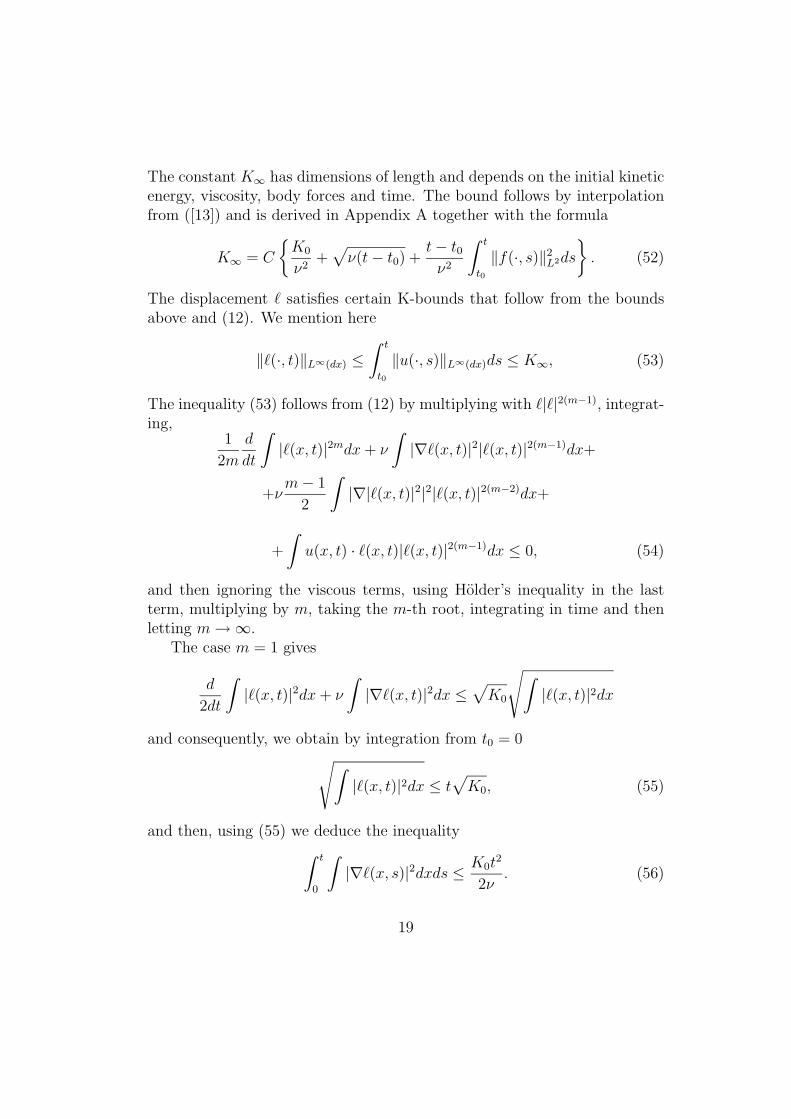
The constant K∞ has dimensions of length and depends on the initial kineticenergy, viscosity, body forces and time. The bound follows by interpolationfrom ([13]) and is derived in Appendix A together with the formula
K∞ = C
{K0
ν2+√ν(t− t0) +
t− t0ν2
∫ t
t0
‖f(·, s)‖2L2ds
}. (52)
The displacement ` satisfies certain K-bounds that follow from the boundsabove and (12). We mention here
‖`(·, t)‖L∞(dx) ≤∫ t
t0
‖u(·, s)‖L∞(dx)ds ≤ K∞, (53)
The inequality (53) follows from (12) by multiplying with `|`|2(m−1), integrat-ing,
1
2m
d
dt
∫|`(x, t)|2mdx+ ν
∫|∇`(x, t)|2|`(x, t)|2(m−1)dx+
+νm− 1
2
∫|∇|`(x, t)|2|2|`(x, t)|2(m−2)dx+
+
∫u(x, t) · `(x, t)|`(x, t)|2(m−1)dx ≤ 0, (54)
and then ignoring the viscous terms, using Holder’s inequality in the lastterm, multiplying by m, taking the m-th root, integrating in time and thenletting m→∞.
The case m = 1 gives
d
2dt
∫|`(x, t)|2dx+ ν
∫|∇`(x, t)|2dx ≤
√K0
√∫|`(x, t)|2dx
and consequently, we obtain by integration from t0 = 0√∫|`(x, t)|2dx ≤ t
√K0, (55)
and then, using (55) we deduce the inequality∫ t
0
∫|∇`(x, s)|2dxds ≤ K0t
2
2ν. (56)
19
Now we multiply (12) by −∆`, integrate by parts, use Schwartz’s inequalityto write
d
dt
∫|∇`(x, t)|2dx+ν
∫|∆`(x, t)|2dx ≤
√∫|∇u(x, t)|2dx
√∫|∇`(x, t)|2dx
−2
∫Trace {(∇`(x, t))(∇u(x, t))(∇`(x, t))∗} dx
and then use the elementary inequality(∫|∇`(x, t)|4dx
) 12
≤ C‖`(·, t)‖L∞(∫|∆`(x, t)|2dx
) 12
,
in conjunction with the Holder inequality and (53) to deduce
d
dt
∫|∇`(x, t)|2dx+ ν
∫|∆`(x, t)|2dx ≤
√∫|∇`(x, t)|2dx
√∫|∇u(x, t)|2dx+ C
K2∞ν
∫|∇u(x, t)|2dx.
We obtain, after integration and use of (43, 56)
∫|∇`(x, t)|2dx+ ν
∫ t
0
∫|∆`(x, s)|2dxds ≤ C
(K0t
ν+K2∞K0
ν2
). (57)
Recalling the bound (49, 50) on kinetic energy we have:
Theorem 1. Assume that the vector valued function ` obeys (12) and as-sume that the velocity u(x, t) is a solution of the Navier-Stokes equations (or,more generally, that it is a divergence-free periodic function that satisfies thebounds (43) and (51)). Then ` satisfies the inequality (53) together with
1
L3
∫|`(x, t)|2dx ≤ (4E0 + tεB)t2, (58)
1
L3t
∫ t
0
∫|∇`(x, s)|2dxds ≤ Bt
2ν, (59)
20
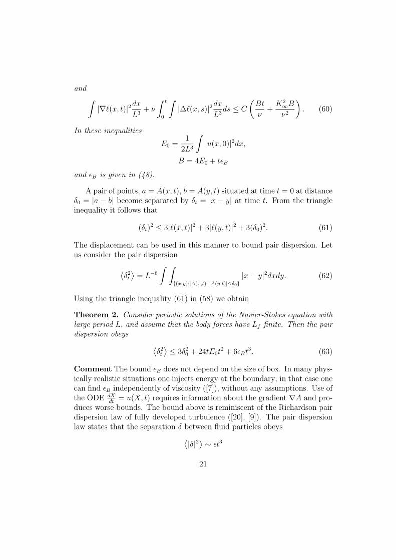
and ∫|∇`(x, t)|2dx
L3+ ν
∫ t
0
∫|∆`(x, s)|2dx
L3ds ≤ C
(Bt
ν+K2∞B
ν2
). (60)
In these inequalities
E0 =1
2L3
∫|u(x, 0)|2dx,
B = 4E0 + tεB
and εB is given in (48).
A pair of points, a = A(x, t), b = A(y, t) situated at time t = 0 at distanceδ0 = |a − b| become separated by δt = |x − y| at time t. From the triangleinequality it follows that
(δt)2 ≤ 3|`(x, t)|2 + 3|`(y, t)|2 + 3(δ0)2. (61)
The displacement can be used in this manner to bound pair dispersion. Letus consider the pair dispersion⟨
δ2t
⟩= L−6
∫ ∫{(x,y);|A(x,t)−A(y,t)|≤δ0}
|x− y|2dxdy. (62)
Using the triangle inequality (61) in (58) we obtain
Theorem 2. Consider periodic solutions of the Navier-Stokes equation withlarge period L, and assume that the body forces have Lf finite. Then the pairdispersion obeys ⟨
δ2t
⟩≤ 3δ2
0 + 24tE0t2 + 6εBt
3. (63)
Comment The bound εB does not depend on the size of box. In many phys-ically realistic situations one injects energy at the boundary; in that case onecan find εB independently of viscosity ([7]), without any assumptions. Use ofthe ODE dX
dt= u(X, t) requires information about the gradient ∇A and pro-
duces worse bounds. The bound above is reminiscent of the Richardson pairdispersion law of fully developed turbulence ([20], [9]). The pair dispersionlaw states that the separation δ between fluid particles obeys⟨
|δ|2⟩∼ εt3
21
where ε is the rate of dissipation of energy and t is time. This is supposedto hold in an inertial range, in statistical steady flux of energy, for timest that are neither too big nor too small and for unspecified initial separa-tions. The “law” can be guessed by dimensional analysis by requiring theanswer to depend solely on time and ε or can be derived using formally theHolder exponent 1/3 for velocity. A rigorous mathematical derivation fromthe Navier-Stokes equations is not available: one is faced with the difficultythat the prediction seems to require both non-Lipschitz, Holder continuousvelocities and a well defined notion of Lagrangian particle paths. LaboratoryLagrangian experiments have only recently begun to be capable of perform-ing precise Lagrangian measurements and a quantitative confirmation of theRichardson law is still not definitive ([19]).
9 ε-bounds
This section is devoted to bounds on higher order derivatives of `. Thesebounds require assumptions. We are going to apply the Laplacian to (12),multiply by ∆` and integrate. We obtain
and we bound ∣∣∣∣∫ Qji(x, t)fj(x, t)vi(x, t)|v(x, t)|2(m−1)dx
∣∣∣∣ ≤{∫|g(x, t)|2mdx
} 12m{∫|v(x, t)|2mdx
} 2m−12m
where
gi(x, t) = Qji(x, t)fj(x, t). (72)
The inequality obtained is
d
dt
∫|v(x, t)|2mdx+ νm(m− 1)
∫|∇|v(x, t)|2|2|v(x, t)|2(m−2)dx ≤
≤ 2mν
∫|C(x, t)|2|v(x, t)|2mdx+
+ 2m
{∫|g(x, t)|2mdx
} 12m{∫|v(x, t)|2mdx
} 2m−12m
(73)
Let us consider for any m ≥ 1 the quantity
q(x, t) = |v(x, t)|m.
The inequality (73) implies
d
dt
∫(q(x, t))2 + 4ν(1− 1
m)
∫|∇q(x, t)|2 ≤ 2mν
∫|C(x, t)|2(q(x, t))2dx+
+ 2m
{∫|g(x, t)|2mdx
} 12m{∫
(q(x, t))2dx
} 2m−12m
Using the well-known Morrey-Sobolev inequality{∫(q(x))6dx
} 13
≤ C0
{∫|∇q(x)|2dx+ L−2
∫(q(x))2dx
}25
and Holder’s inequality we deduce
d
dt
∫(q(x, t))2 + 4ν(1− 1
m)
∫|∇q(x, t)|2 ≤
≤ 2mνC0
{∫|C(x, t)|3dx
} 23{∫|∇q(x, t)|2dx+ L−2
∫(q(x, t))2dx
}
+ 2m
{∫|g(x, t)|2mdx
} 12m{∫
(q(x, t))2dx
} 2m−12m
Assume that, on the time interval t ∈ [0, τ ], C(x, t) obeys the smallnesscondition {∫
|C(x, t)|3dx} 1
3
≤
√2(m− 1)
C0m2(74)
for m > 1 or {∫|C(x, t)|3dx
} 13
≤√
1
4C0
(75)
for m = 1. Then
d
dt‖v(·, t)‖L2m ≤ ν(m− 1)
2m2L2‖v(·, t)‖L2m + ‖g(·, t)‖L2m
for t ∈ [0, τ ] and consequently
‖v(·, t)‖L2m ≤ ‖v0‖L2meν(m−1)t
2m2L2 +
∫ t
0
‖g(·, s)‖L2m (76)
holds on the same time interval.
11 Bounds for the virtual vorticity
We take here the body forces equal to zero, and start directly with the point-wise inequality (42). Multiplying by m|ζ|2(m−1) and integrating we obtain,as above
d
dt
∫(q(x, t))2 + 4ν(1− 1
m)
∫|∇q(x, t)|2 ≤ 17mν
∫|C(x, t)|2(q(x, t))2dx
26
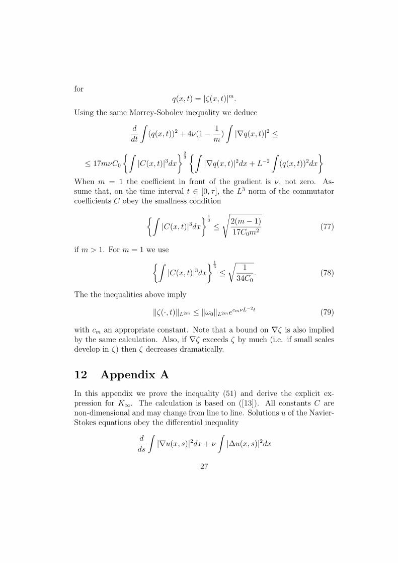
forq(x, t) = |ζ(x, t)|m.
Using the same Morrey-Sobolev inequality we deduce
d
dt
∫(q(x, t))2 + 4ν(1− 1
m)
∫|∇q(x, t)|2 ≤
≤ 17mνC0
{∫|C(x, t)|3dx
} 23{∫|∇q(x, t)|2dx+ L−2
∫(q(x, t))2dx
}When m = 1 the coefficient in front of the gradient is ν, not zero. As-sume that, on the time interval t ∈ [0, τ ], the L3 norm of the commutatorcoefficients C obey the smallness condition{∫
|C(x, t)|3dx} 1
3
≤
√2(m− 1)
17C0m2(77)
if m > 1. For m = 1 we use{∫|C(x, t)|3dx
} 13
≤√
1
34C0
. (78)
The the inequalities above imply
‖ζ(·, t)‖L2m ≤ ‖ω0‖L2mecmνL−2t (79)
with cm an appropriate constant. Note that a bound on ∇ζ is also impliedby the same calculation. Also, if ∇ζ exceeds ζ by much (i.e. if small scalesdevelop in ζ) then ζ decreases dramatically.
12 Appendix A
In this appendix we prove the inequality (51) and derive the explicit ex-pression for K∞. The calculation is based on ([13]). All constants C arenon-dimensional and may change from line to line. Solutions u of the Navier-Stokes equations obey the differential inequality
d
ds
∫|∇u(x, s)|2dx+ ν
∫|∆u(x, s)|2dx
27
≤ C
ν3
(∫|∇u(x, s)|2dx
)3
+C
ν
∫|f(x, s)|2dx.
The idea of ([13]) was to divide by an appropriate quantity to make use ofthe balance (43). The quantity is
(G(s))2 =
(γ2 +
∫|∇u(x, s)|2dx
)2
where γ is a positive constant that does not depend on s and will be specifiedlater. Dividing by (G(s))2, integrating in time from t0 to t and using (43)one obtains ∫ t
t0
‖∆u(·, s)‖2L2(G(s))−2ds ≤
C
(K0
ν5+
1
νγ2+
1
ν2γ4
∫ t
t0
‖f(·, s)‖2ds
).
The three dimensional Sobolev embedding-interpolation inequality for peri-odic mean-zero functions
‖u‖L∞ ≤ C‖∇u‖12
L2‖∆u‖12
L2
is elementary. From it we deduce
‖u(·, s)‖L∞ ≤ C‖∇u(·, s)‖12
L2(G(s))12
[‖∆u(·, s)‖L2G(s)−1
] 12
Integrating in time, using the Holder inequality, the inequality (43) and theinequalities above we deduce∫ t
t0
‖u(·, s)‖L∞ ≤ Cr
where the length r = r(γ, t, ν,K0) is given in terms of six length scales
K0
ν2= r0,
ν2
γ2= r1,
(t− t0)γ2
ν= r2,
(γ(t− t0))23 = r3,
t− t0ν2
∫ t
t0
‖f(·, s)‖2L2ds = r4
andr5 =
√ν(t− t0).
28
The expression for r is
r = r0 + (r0)34 (r1)
14 + (r0)
12 (r2)
12 + (r0)
14 (r3)
34 +
(r0)14 (r4)
14 (r5)
12 + (r0)
34 (r4)
14
(r1
r2
) 14
The choice
γ4 =ν3
t− t0entrains
r1 = r2 = r3 = r5
reducing thus the number of length scales to three, the energy viscous lengthscale r0, the diffusive length scale r5 and the force length scale r4. The boundbecomes
K∞ = C(r0 + r4 + r5)
i.e. (52).
13 Appendix B
We prove her the commutation relation (16). We take an arbitrary functiong and compute [Γ, Lig]) where Γ = Γν(u,∇) and Li = ∇i
A. We use first (10):
[Γ, Lig] = Γ (Qji∂jg)−Qji∂jΓg =
Γ(Qji)∂jg +QjiΓ∂jg − 2ν∂k(Qji)∂k∂jg −Qji∂jΓg =
(commuting in the last term ∂j and Γ)
Γ(Qji)∂jg − 2ν∂k(Qji)∂k∂jg −Qji∂j(uk)∂kg =
(changing names of dummy indices in the last term)
(Γ(Qji)−Qki∂k(uj)) ∂jg − 2ν∂k(Qji)∂k∂jg =
(using (15))
2νQjp(∂l∂kAp)(∂kQli)∂jg − 2ν∂k(Qji)∂k∂jg =
29
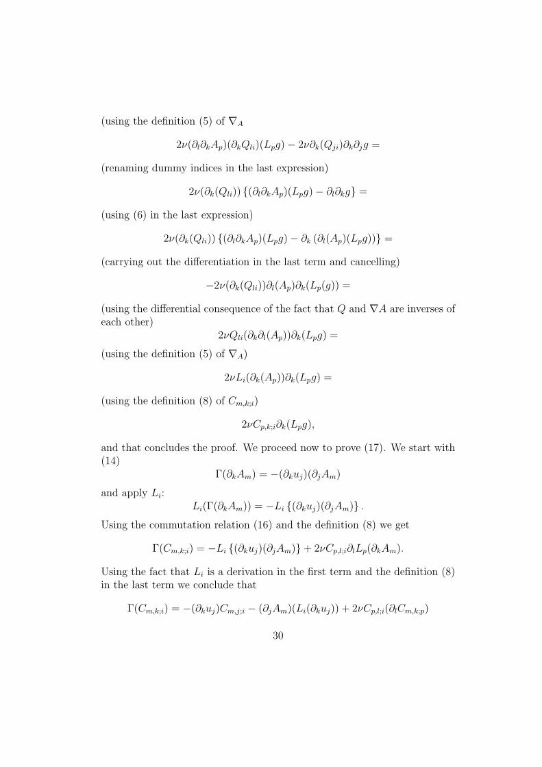
(using the definition (5) of ∇A
2ν(∂l∂kAp)(∂kQli)(Lpg)− 2ν∂k(Qji)∂k∂jg =
(renaming dummy indices in the last expression)
2ν(∂k(Qli)) {(∂l∂kAp)(Lpg)− ∂l∂kg} =
(using (6) in the last expression)
2ν(∂k(Qli)) {(∂l∂kAp)(Lpg)− ∂k (∂l(Ap)(Lpg))} =
(carrying out the differentiation in the last term and cancelling)
−2ν(∂k(Qli))∂l(Ap)∂k(Lp(g)) =
(using the differential consequence of the fact that Q and ∇A are inverses ofeach other)
2νQli(∂k∂l(Ap))∂k(Lpg) =
(using the definition (5) of ∇A)
2νLi(∂k(Ap))∂k(Lpg) =
(using the definition (8) of Cm,k;i)
2νCp,k;i∂k(Lpg),
and that concludes the proof. We proceed now to prove (17). We start with(14)
Γ(∂kAm) = −(∂kuj)(∂jAm)
and apply Li:Li(Γ(∂kAm)) = −Li {(∂kuj)(∂jAm)} .
Using the commutation relation (16) and the definition (8) we get
which is (17). We compute now the formal adjoint of ∇iA
(∇iA)∗g = −∂j(Qjig) = −∇i
A(g)− (∂j(Qji))g
(with (6))(∇i
A)∗g = −∇iA(g)− {(∂jAp)Lp(Qji)} g =
(using the fact that Q is the inverse of ∇A)
(∇iA)∗g = −∇i
A(g) +QjiCp,j;pg.
Acknowledgments. This work is a continuation of research startedwhile the author was visiting the Department of Mathematics of PrincetonUniversity, partially supported by an AIM fellowship. Part of this workwas done at the Institute for Theoretical Physics in Santa Barbara, whosehospitality is gratefully acknowledged. This research is supported in part byNSF- DMS9802611.
References
[1] T. F. Buttke, Velicity methods: Lagrangian methods which preservethe Hamiltonian structure of incompressible flow, in Vortex flows andrelated numerical methods, NATO Adv. Sci. Inst. Ser. C Math. Phys.Sci. 395, J.T. Beale edtr, Kluwer Boston (1993), 39.
[2] Shiyi Chen, Ciprian Foias, Darryl D Holm, Eric Olson, Edriss S Titi,Shannon Wynn, A connection between the Camassa-Holm equationsand turbulent flows in channels and pipes, Phys. Fluids, 11 (1998),2343-2353.
[3] A. J. Chorin, Vortex phase transitions in 2 1/2 dimensions, J. Stat. Phys76 (1994), 835.
[4] P. Constantin, An Eulerian-Lagrangian approach for incompressible flu-ids: Local theory, http://arXiv.org/abs/math.AP/0004059.
[5] P.Constantin, An Eulerian-Lagrangian approach to fluids, preprint 1999,(www.aimath.org).
[6] P. Constantin, C. Foias, Navier-Stokes equations, University of ChicagoPress, Chicago, 1988.
31
[7] C. Doering, P. Constantin, Energy dissipation in shear driven turbu-lence, Phys.Rev.Lett. 69 (1992), 1648-1651.
[8] W. E, J. G. Liu, Finite difference schemes for incompressible flows inthe velocity-impulse density formulation, J. Comput. Phys. 120 (1997),67-76.
[9] U. Frisch, Turbulence, Cambridge Univ ersity Press, Cambridge, 1995.
[10] S. Gama, U. Frisch, Local helicity, a material invariant for the odd-dimensional incompressible Euler equations, in NATO-ASI Theory ofsolar and planetary dynamos M.R.E. Proctor edtr, Cambridge U. Press,Cambridge (1993), 115.
[11] M. E. Goldstein, Unsteady vortical and entropic distortion of potentialflows round arbitrary obstacles, J. Fluid Mech. 89 (1978), 433-468.
[12] M. E. Goldstein, P. A. Durbin, The effect of finite turbulence spatialscale on the amplification of turbulence by a contracting stream, J. FluidMech. 98 (1980), 473-508.
[13] C. Guillope, C. Foias, R. Temam, New a priori estimates for the Navier-Stokes equations in dimension 3, Commun. PDE 6 (1981),329-359.
[14] D. D. Holm, Lyapunov stability of ideal compressible and incompress-ible fluid equilibria in three dimensions, in Sem. Math. Sup. 100, Univ.Montreal Press, Montreal (1986), 125.
[15] D.D. Holm, J. E. Marsden, T. Ratiu, Euler-Poincare models of idealfluids with nonlinear dispersion, Phys. Rev. Lett. 349 (1998), 4173-4177.
[16] J. C. R. Hunt, Vorticity and vortex dynamics in complex turbulent flows,Transactions of CSME, 11 (1987), 21-35.
[17] G. A. Kuzmin, Ideal incompressible hydrodynamics in terms of the vor-tex momentum density, Phys. Lett 96 A (1983), 88-90.
[18] J. J. Maddocks, R.L. Pego, An unconstrained Hamiltonian formulationfor incompressible fluid flows, Commun. Math. Phys. 170 (1995), 207.
32
[19] J. Mann, S. Ott and J.S. Andersen, Experimental study of relative tur-bulent diffusion, Riso National Laboratory, Denmark Riso-R-1036(EN)(1999).
[20] A. S. Monin and A. M. Yaglom, Statistical Fluid Mechanics M.I.T. Press,Cambridge, 1987.
[21] V. I. Oseledets, On a new way of writing the Navier-Stokes equation.The Hamiltonian formalism, Commun. Moscow Math. Soc. (1988), Russ.Math. Surveys 44 (1989), 210 -211.
[22] P. Roberts, A Hamiltonian theory for weekly interacting vortices, Math-ematica 19 (1972), 169-179.
[23] G. Russo, P. Smereka, Impulse formulation of the Euler equations: gen-eral properties and numerical methods, J. Fluid Mech. 391 (1999), 189-209.
[24] J. Serrin, Mathematical principles of classical fluid mechanics, (S.Flugge, C. Truesdell Edtrs.) Handbuch der Physik, 8 (1959), 125 -263,p.169.
[25] A. V. Tur, V. V. Yanovsky, Invariants in dissipationless hydrodynamicmedia, J. Fluid Mech. 248 (1993), 67.


![Eulerian-Lagrangian Formulation for Compressible Navier ......Eulerian-Lagrangian Formulation for Compressible Navier-Stokes Equations 3 [ ,D t] ( u ) · , (10) we can obtain the evolution](https://static.documents.pub/doc/80x56/60aae98a3d03cb7e180eb311/eulerian-lagrangian-formulation-for-compressible-navier-eulerian-lagrangian.jpg)


