AN EVALUATION OF A PRESENCE-ABSENCE SURVEY TO MONITOR MONTEZUMA QUAIL IN WESTERN TEXAS A Thesis by CRISTELA GONZALEZ SANDERS Submitted to the College of Graduate Studies Texas A&M University-Kingsville in partial fulfillment of the requirements for the degree of MASTER OF SCIENCE August 2012 Major Subject: Range and Wildlife Management
Transcript
AN EVALUATION OF A PRESENCE-ABSENCE SURVEY TO MONITOR
MONTEZUMA QUAIL IN WESTERN TEXAS
A Thesis
by
CRISTELA GONZALEZ SANDERS
Submitted to the College of Graduate Studies Texas A&M University-Kingsville
in partial fulfillment of the requirements for the degree of
MASTER OF SCIENCE
August 2012
Major Subject: Range and Wildlife Management
AN EVALUATION OF A PRESENCE-ABSENCE SURVEY TO MONITOR
(Chairman of Committee) ______________________________ ______________________________ Leonard A. Brennan, Ph.D. Louis A. Harveson, Ph.D. (Member) (Member) ______________________________ ______________________________
Robert M. Perez Scott E. Henke, Ph.D. (External Member) (Head of Department)
and Del Rio Route (n = 20 survey points) for July–August 2008. If points within a
xi
single habitat type did not have a single detection throughout the 5 surveys, they were
removed because analysis was not reaching convergence (n = 25 survey points)…..102
VITA ............................................................................................................................... 109
xii
LIST OF FIGURES Figure 1. Elephant Mountain Wildlife Management Area (TX) terrain, 18 July 2008. .. 13 Figure 2. Alpine grasslands dominated by native grasses on plateau at Elephant Mountain Wildlife Management Area (TX), 15 July 2008. ............................................. 14 Figure 3. Woody and grassland vegetation at Davis Mountains Preserve (TX), 6 August 2007................................................................................................................................... 16 Figure 4. Uvalde Route (TX) (n = 25 survey points), where callback surveys were conducted during July–August 2008. ............................................................................... 18 Figure 5. Aerial map of Elephant Mountain Wildlife Management Area that was used for callback surveys and vegetation sampling during July–August 2007. ............................. 21 Figure 6. Davis Mountains Preserve (n = 20 survey points), there were additional points on the Davis Mountains Preserve (n = 10) not shown on this map. Callback surveys were conducted during July–August 2008 in different vegetation communities. ..................... 23 Figure 7. Del Rio Road Route (TX) (n = 20 survey points), callback surveys were conducted during July–August 2008. ............................................................................... 24 Figure 8. Example how profile board and Robel pole measurements were conducted at Davis Mountains Preserve (TX), 5 August 2008. ............................................................. 28 Figure 9. A) Allium sp. with flower found at Davis Mountain Preserve (TX), 15 April 2007. B) Allium sp. without flower found at Elephant Mountain Wildlife Management Area (TX), 28 July 2007. .................................................................................................. 29 Figure 10. Oxalis sp. found at Davis Mountains Preserve (TX), 4 August 2007. ........... 30 Figure 11. Cyperus sp. found at Davis Mountains Preserve (TX), 29 July 2007. ........... 31
xiii
Figure 12. Texas Parks and Wildlife Department Vegetation types of Texas used to
distinguish vegetation types for callback surveys in 2008 survey season (TPWD 2000c).
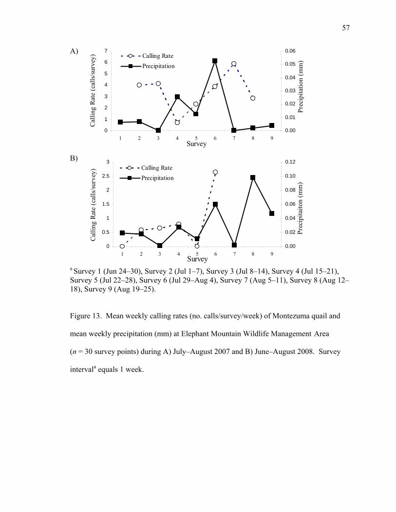
........................................................................................................................................... 32 Figure 13. Mean weekly calling rates (no. calls/survey/week) of Montezuma quail and mean weekly precipitation (mm) at Elephant Mountain Wildlife ManagementArea ....... 57 Figure 14. Mean weekly calling rates (no. calls/survey/week) of Montezuma quail and mean weekly precipitation (mm) at Davis Mountains Preserve (n = 30 survey points) during A) July–August 2007 and B) June–August 2008. Survey intervala equals 1 week. ........................................................................................................................................... 58 Figure 15. Probability of detection and vegetation height (dm) at Elephant Mountain Wildlife Management Area (n = 30 survey points) during A) July–August 2007 and B) June–August 2008. ............................................................................................................ 66 Figure 16. Probability of detection and vegetation height (dm) at Davis Mountains Preserve (n = 30 survey points) during A) July–August 2007 and (n = 10 survey points) during B) June–August 2008. ........................................................................................... 67 Figure 17. Probability of detection and vegetation height (dm) at Elephant Mountain Wildlife Management Area (n = 30 survey points in 2007, and n = 30 survey points in 2008) and Davis Mountains Preserve (n = 30 survey points in 2007 and n = 10 survey points in 2008) during A) July–August 2007 and B) June–August 2008. ........................ 68 Figure 18. Predictive map of occurrence of Montezuma quail based on vegetation type and elevation in west Texas. ............................................................................................. 71
xiv
LIST OF TABLES Table 1. Habitat variables measured during survey season 2007 and 2008 with indication
of whether they were removed from the analysis. ............................................................ 35
Table 2. Analysis 1 a priori occupancy models for Program PRESENCE based on
micro-scale habitat characteristics. All model combinations for analysis are shown. ..... 39
Table 3. Analysis 1 a priori detection models for Program PRESENCE at a micro-scale
based on weather variables and vegetation height. All model combinations for analysis
are shown. ......................................................................................................................... 40
Table 4. Analysis 2 a priori detection models for Program PRESENCE at a micro-scale
based on weather variables and vegetation height. All model combinations for analysis
are shown. ......................................................................................................................... 42
Table 5. Analysis 3 a priori occupancy models for Program PRESENCE based on
macro-scale habitat characteristics to develop predictive distribution map. All model
combinations for analysis are shown ................................................................................ 43
Table 6. Analysis 3 a priori detection models for Program PRESENCE based on weather
variables. All model combinations for analysis are shown. ............................................. 46
Table 7. Monthly mean ( ) weather variables (temperature, wind, and humidity) for
Elephant Mountain Wildlife Management Area (Elephant Mountain WMA), Davis
Mountains Preserve (Davis MP), Del Rio Route (DRR), and Uvalde Road Route (UVR)
for July–August 2007 (N = 150 surveys/study site) and June–August 2008 (N = 150
surveys/study site). Units for temperature are Celsius (°C), wind (km/hr) and humidity
Table 14. Analysis 1 top 10 a priori microhabitat models for Montezuma quail evaluated
using Akaike’s Information Criterion (AIC) in Program PRESENCE 2.3. Models
evaluated occupancy (psi) as a function of 3 micro- habitat variables (food-plant density
[m2], percent grass cover, and vegetation height [cm]) and probability of detection (p) as
a function of weather (time, temperature, and wind), survey date, and vegetation height
[dm]. The AIC values, relative differences in AIC (Δ AIC), AIC model weights (w),
xvii
model likelihood (AIC weight divided by the AIC weight of the best model), and number
of parameters (K) are given for each model. Models are for Elephant Mountain Wildlife
Management Area and Davis Mountains Preserve subset data (n = 40 survey points) for
June–August, 2007 and July–August 2008. ...................................................................... 63
Table 15. Analysis 2 top 10 a priori weather and vegetation height models (Analysis 2)
for Montezuma quail evaluated using Akaike’s Information Criterion (AIC) in Program
PRESENCE 2.3. Models evaluated probability of detection (p) as a function of the
constant function, survey specific function, and weather (time [am/pm], temperature [°F],
wind [mph] and vegetation height [dm]. The AIC values (AIC), relative differences in
AIC (Δ AIC), AIC model weights (w), model likelihood (AIC weight divided by the AIC
weight of the best model), and the number of parameters (K) are given for each model.
Models are for Elephant Mountain Wildlife Management Area (n = 30 survey points),
Davis Mountains Preserve (n = 30 survey points) in June–August 2007. ........................ 65
Table 16. Analysis 3 top 10 a priori macro-models for Montezuma quail evaluated using
Akaike’s Information Criterion (AIC) in Program PRESENCE 2.3. Models evaluated
occupancy (psi) as a function of 5 macrohabitat variables (habitat- suitability type [High,
Moderate, or Low], slope [°], and elevation [m]), and probability of detection (p) as a
constant function, survey specific function, and weather (time [am/pm], temperature [°F],
and wind [mph]). The AIC values (AIC), relative differences in AIC (Δ AIC), AIC model
weights (w), model likelihood (AIC weight divided by the AIC weight of the best model),
and the number of parameters (K) are given for each model. Models are for Elephant
Mountain Wildlife Management Area (n = 30 survey points), Davis Mountains Preserve
(n = 30 survey points), Uvalde Road Route (n = 25 survey points), and Del Rio Route (n
xviii
= 20 survey points) for July–August 2008. If points within a single habitat type did not
have a single detection throughout the 5 surveys, they were removed because analysis
was not reaching convergence (n = 25). ........................................................................... 69
1
CHAPTER I BACKGROUND ON MONTEZUMA QUAIL Literature Review on Life History and Ecology
Movements.—Montezuma quail populations are found in suitable habitats in
Arizona, New Mexico, and Texas south along Sierra Madre woodlands of Mexico to
Oaxaca (Stromberg 2000). During the breeding season (Feb–Sep) pairs will generally
remain well spaced over the habitat usually distanced 100–200 m apart (Stromberg
2000). During nesting season and winter (Aug–Jan), adults with young remain in coveys,
often feeding, walking, and resting within a few square meters of each other (Stromberg
2000). The size of the covey’s home range varies depending on the size of the covey and
the number of coveys in an area but on average it is about 5.67–6.07 ha (Brown 1976).
No seasonal migrations in elevations or long-distance movements have been documented
with data from band recoveries or observations of individually marked birds (Stromberg
2000).1
Food habits.—Montezuma quail forage primarily by digging for underground
plant organs, such as rhizomes and tubers of flatsedges (Cyperus spp.) and corms of
woodsorrels (Oxalis spp.) (Bristow and Ockenfels 2000). Food selection changes
seasonally with roots and tubers eaten year-round. Acorns (Quercus spp.) may be taken
during the dry season when available, and with monsoonal rains, insects become the
dominant food source (Stromberg 2000). Insects consumed during the summer are
grasshoppers (Orthoptera), ants (Formicidae), and beetles (Coleoptera) (Bishop1964,
Bishop and Hungerford 1965, Brown 1978). During the fall, a variety of seeds such as
panic grass (Panicum spp.), morning glory (Ipomoea spp.), nightshade (Solanum spp.), This thesis follows the style of Journal of Wildlife Management.
2
brodiaea (Brodiaea spp.), yucca (Yucca spp), and lupine (Lupinus spp.) are consumed,
this reflects the abundance of food items available (Stromberg 2000). Montezuma quail
do not need to drink free standing water (Stromberg 2000). Adults rarely drink water, but
chicks drink more often (Stromberg 2000). Underground plant organs consumed by
Montezuma quail contain high water content and probably represent an important source
of water for this bird (Holdermann and Holdermann 1998).
Habitat.—Bristow and Ockenfels (2004) found that during the pairing season
(Apr–Jun), Montezuma quail prefer oak (Quercus spp.) -woodland habitats that contain a
minimum tree canopy of 26% and grass canopy of 51–75% cover at 20-cm height to
provide optimum cover availability. Montezuma quail can exist in areas with relatively
few oak trees, although quail densities are often lower than typical in oak-woodland
habitat (Bristow and Ockenfels 2000). Montezuma quail are dependent upon perennial
bunch grasses for escape, thermal cover, and for nest construction (Wallmo 1954,
Leopold and McCabe 1957, Bishop 1964, Brown 1978). Livestock grazing and cover
availability are considered important factors affecting Montezuma quail distribution and
density (Bristow and Ockenfels 2004).
Population Estimation Techniques
Auditory counts.—Audio playback techniques have been successful in luring,
capturing, and surveying a variety of birds (Johnson et al. 1981). Sorola (1986) stated
that auditory playbacks may be suitable for presence-absence surveys for Montezuma
quail. Females produce a musical descending call that is owl-like, or a quavering series
of metallic whistles with an average of 9 separate notes slowly descending in pitch which
is referred to as the flock assembly call (Fuentes 1903, Swarth 1909, Leopold and
3
McCabe 1957, Levy et al. 1966, Brown 1976). This call is much louder and lower-
pitched during breeding season (Bishop 1964). Buzz calls are only produced by males; it
is an “insect-like” descending whistle combined with a buzz that has an intangible
quavering quality (Bishop 1964, Stromberg 2000). Buzz calls can be heard up to 200 m
in quiet, calm conditions (Bishop 1964, Brown 1976). Bishop (1964) and Levy et al.
(1966) found that females produce descending calls in early mornings and evenings.
Males within 200–300 m respond with a buzz call and approach the calling female
(Stromberg 2000). During monsoons of July–September, females and males call
throughout the day (Levy et al. 1966, Brown 1976). Males return buzz calls when
recordings are played; individual males reveal their location as they respond to playback
of previously recorded buzz calls (Levy et al. 1966).
Line and point transects.—Due to the Montezuma quail’s cryptic plumage
coloration and “freeze” behavior, it is almost impossible to conduct any type of line
transects or point transects to survey this species. Males have bright, contrasting
plumage; however, they are almost always invisible in their grassland habitats
(Stromberg 2000). Individuals often are first detected as they leap straight up from the
observer’s feet (Stromberg 2000). One can hike for days in suitable habitat and never
observe these quail, unknowingly walking past many coveys (Stromberg 2000). Thus,
traditional survey methods used for other quail species such as Gambel’s quail
(Callipepla gambelii) and scaled quail (C. squamata) do not perform well when used on
Montezuma quail (Bristow and Ockenfels 2000).
Trapping and bird dogs.—Some of the trapping techniques for Montezuma quail
were compared by Hernández et al. (2006) in the Chihuahuan Desert. Funnel traps,
4
modified funnel traps, and feeding stations were evaluated for capturing Montezuma
quail. However, they were unable to capture Montezuma quail using funnel traps or
modified funnel traps despite seeing Montezuma quail in the immediate region. Pre-
baiting had no significant effect in trapability (Hernández et al. 2006). Stromberg (1990)
on the other hand was able to trap Montezuma quail using funnel traps but reported a low
capture success (0.008–0.012 birds/trap-day). Brown (1976) used dogs for surveying and
capturing Montezuma quail. Other researchers have implemented modifications to
Brown’s technique for determining distribution and abundance of Montezuma quail
(Holdermann 1992, Bristow and Ockenfels 2000). Survey methods, such as mark-
recapture and using indirect scratch signs, also proved unsuccessful for Montezuma quail
(Bristow and Ockenfels 2000).
Occupancy modeling.―The use of presence-absence information to monitor
spatial and temporal changes in wildlife populations has a long history; however, until
recently, its application has been limited (Vojta 2005). Presence-absence information has
been difficult to interpret because animal detectability is not constant in time or space
(Vojta 2005). Geissler and Fuller (1987) were the first to propose that detection
probabilities could be estimated from repeated surveys at the same sites. Azuma et al.
(1990) showed that trials across a randomized sample of sites could be used to estimate
the proportion of sites occupied by a species while adjusting for imperfect detection.
Zielinski and Stauffer (1996) incorporated home-range size into sampling unit
distribution and used a simulation model to estimate the sample sizes needed to observe
specified levels of decline in populations for fishers (Martes pennanti) and American
martens (M. americana) (Vojta 2005). Nichols and Karanth (2002) recommended
5
treating sites as individual animals. The detection-nondetection history became
equivalent to capture-recapture data in the model. MacKenzie et al. (2002) made a major
contribution to presence-absence information by demonstrating that detection histories
could be incorporated directly into a maximum likelihood estimation model resulting in
the simultaneous estimate of detection probabilities and occupancy rates.
Recent developments in presence-absence monitoring approaches may provide an
effective method for monitoring Montezuma quail populations. In a monitoring context,
using the presence-absence technique, the proportion of monitoring sites (i.e., habitat
patches or quadrants) within a region where species is present can be used as an index for
population size or species abundance. This is particularly true at large scales, for cryptic,
low-density and/or territorial species (MacKenzie 2005). The ability to estimate changes
in occupancy between two time periods has implications for exploring metapopulation
dynamics (Vojta 2005). Rates of colonization and local extinction can now be estimated
and relationships can be formally tested between colonization rates and isolation of
landscape patches, and between extinction rates and patch sizes (Vojta 2005).
6
LITERATURE CITED Azuma, D. L., J. A. Baldwin, and B. R. Noon. 1990. Estimating the occupancy of
spotted owl habitat areas by sampling and adjusting for bias. General Technical
Report PSW-124. U. S. Forest Service, Berkeley, California, USA.
Bishop, R. A. 1964. The Mearns quail (Cyrtonyx montezumae mearnsi) in southern
Arizona. M.S. Thesis, University of Arizona, Tuscon.
Bishop, R.A. and C.R. Hungerford. 1965. Seasonal food selection of Arizona
Mearns’quail. Journal of Wildlife Management 29:813–819.
Bristow, K. D., and R. A. Ockenfels. 2000. Effects of human activity and habitat
conditions on Mearns’ quail populations. Federal Aid in Wildlife Restoration
Project W-78-R. Arizona Game and Fish Department Research Branch Technical
Guidance, Bulletin No. 4, Phoenix, USA.
Bristow, K. D., and R. A. Ockenfels. 2004. Pairing season habitat selection by
Montezuma quail in southeastern Arizona. Journal of Wildlife Management
57:532–538.
Brown, R. L. 1976. Mearns’ quail census technique. Federal Aid in Wildlife
Restoration Project W-78-R-15, Work Plan 1, Job 1. Arizona Game and Fish
Department, Phoenix, Arizona, USA.
Brown, R.L. 1978. An ecological study of Mearn’s quail. Arizona Game and Fish
Department Federal Aid in Wildlife Restoration final report. Project W-78-R-22,
Phoenix. Arizona.
Fuentes, L. A. 1903. With the Mearns quail in southwestern Texas. Condor 5:113–116.
7
Geissler, P. H., and M. R. Fuller. 1987. Estimation of the proportion of an area occupied
by an animal species. Proceedings of the Section on Survey Research Methods of
the American Statistical Association 1986:533-538.
Hernández, F., L. A. Harveson, and C. Brewer. 2006. A comparison of trapping
techniques for Montezuma quail. Wildlife Society Bulletin 34:1212–1215.
Holdermann, D. A. 1992. Montezuma quail investigations. New Mexico Game and
Fish Department Professional Servides Contract 80-516-41-83, Santa Fe, USA.
Holdermann, D.A. and R. Holdermann. 1998. Some aspects of the ecology of yellow
nutsedge, Gray’s woodsorrel and pocket gophers in relation to Montezuma Quail
in the Sacramento Mountains, New Mexico. New Mexico Ornithological Society
Bulletin 26: 31.
Johnson, R. R., B. T. Brown, L. T. Haight, and J. M. Simpson. 1981. Playback
recordings as a special avian censusing technique. Pages 66–75 in C. J. Ralph and
J. M. Scott, editors. Estimating the numbers of terrestrial birds. Cooper
Ornithological Society, Studies in Avian Biology No. 6. Allen. Lawrence,
Kansas, USA.
Leopold, S., and R. A. McCabe. 1957. Natural history of the Montezuma quail in
Mexico. Condor 59:3–26.
Levy, S. H., J. J. Levy, and R. A. Bishop. 1966. Use of tape recorded female quail calls
during the breeding season. Journal of Wildlife Management 30:426–428.
MacKenzie, D. 2005. What are the issues with Present-Absence data for wildlife
managers? Journal of Wildlife management 69:849–860.
8
Mackenzie, D. I., J. D. Nichols, G. B. Lachman, S. Droege, J. A. Royle, C. A.
Langtimm. 2002. Estimating site occupancy rates when detection probabilities
are less than one. Ecology 83:2248–2255.
Nichols, J. D., and K. U. Karanth. 2002. Statistical concepts: assessing spatial
distributions. Pages 29–38 in K. U. Karanth and J. D. Nichols, editors.
Monitoring tigers and their prey: a manual for wildlife managers, researchers, and
conservationists. Centre for Wildlife Studies, Bangalore, India.
Olson, G. S., R. G. Anthony, E. D. Forsman, S. H. Ackers, P. J. Loschl, J. A. Reid, K.
M. Dugger, E. M. Glenn, and W. J. Ripple. 2005. Modeling of site occupancy
dynamics for northern spotted owls, with emphasis on the effects of barred owls.
Journal of Wildlife Management 69:918–932.
Sorola, S. K. 1986. Investigation of Mearns’ quail distribution. Texas Parks and
Wildlife Department Final Report Project W-108-R-9, Austin, USA.
Stromberg, M. R. 1990. Habitat, movements and roost characteristics of Montezuma
quail in southeastern Arizona. Condor 92:229–236.
Stromberg, M. R. 2000. Montezuma quail (Cyrtonyx montezumae). Account 524 in A.
Poole and F. Gill, editors. The birds of North America. The Academy of Natural
Sciences, Philadelphia, Pennsylvania, and The American Ornithologists’ Union,
Washington, D. C., USA.
Swarth, H. S. 1909. Distribution and molt of the Mearns quail. Condor 11:39–43.
Vojta, C.D. 2005. Old dog, new tricks: innovations with presence-absence information.
Journal of Wildlife Management 69:845–848.
9
Wallmo, O.C. 1954. Nesting of Mearns quail in southeastern Arizona. Condor 56:125–
128.
Zielinski, W. J., and H. B. Stuffer. 1996. Monitoring Martes populations in California:
survey design and power analysis. Ecological Applications 6:1254–1267.
10
CHAPTER II
AN EVALUATION OF PRESENCE-ABSENCE SURVEYS TO MONITOR
MONTEZUMA QUAIL IN WESTERN TEXAS
INTRODUCTION The secretive nature and cryptic plumage of Montezuma quail (Cyrtonyx montezumae)
makes obtaining basic ecological information on this species difficult. Very little data
currently exist on the ecology or population status of Montezuma quail in Texas
(Hernández et al. 2006a, Harveson et al. 2007). This lack of knowledge is problematic
because the range and population size of Montezuma quail have declined over the past
century (Oberholser 1974, Gehlbach 1981).
Several challenges have impeded the development of an effective population
monitoring program for Montezuma quail such as their occurrence on vast, inaccessible
landscapes, relatively low densities, and low detectability. Researchers have attempted to
develop monitoring techniques for the species but have had limited success (Brown 1976,
Bristow and Ockenfels 2000, Robles et al. 2002, Hernández et al. 2006b). These have
included call counts, dig counts, maps of foraging signs, line drive techniques, radio
telemetry, and mark-recapture (Brown 1976, Bristow and Ockenfels 2000, Stromberg
2000, Robles et al. 2002, Harveson et al. 2006, Hernández et al. 2006b,). 2
Recent advancements in monitoring techniques involving the use and application
of presence-absence information can provide a practical solution for reliably monitoring
rare or elusive species over large scales (Thompson 2004, MacKenzie et al. 2005).
Geissler and Fuller (1987) proposed that data from repeated surveys to the same sites
could be used to estimate detection probabilities, and Azuma et al. (1990) demonstrated This thesis follows the style of Journal of Wildlife Management.
11
that repeat site visits could also be used to estimate occupancy (i.e., proportion of sites
occupied by a species) while accounting for imperfect detection. The ability to obtain
unbiased occupancy estimates has implications from a monitoring perspective because
occupancy can be used as a surrogate for population size, particularly for cryptic or low-
density species at large scales (MacKenzie 2005, Vojta 2005). In addition, occupancy
estimation permits proper characterization of habitat models and resource selection
functions (Vojta 2005, MacKenzie 2006).
Given recent theoretical developments of presence-absence surveys, the use of
occupancy estimation for monitoring Montezuma quail populations’ warrants evaluation.
The purpose of my research was to use a presence-absence approach to estimate
occupancy and detection probability of Montezuma quail in Texas. If the call-back
surveys are conducted during June–August, then, they can be used as a tool to monitor
Montezuma quail distributions. Specifically, the main objectives were to:
1. Estimate occupancy rate and detection probability of Montezuma quail
using presence-absence information obtained via repeated, call-back
surveys;
2. Evaluate relationships between calling rate of Montezuma quail with
precipitation; and
3. Develop a distribution map based on resource-selection functions for
Montezuma quail that describe the probability of occupancy as a
function of habitat characteristics.
12
STUDY AREA My study was conducted on 4 study areas: 1) Elephant Mountain Wildlife Management
Area (Elephant Mountain WMA; Brewster County), 2) Davis Mountain Preserve of The
Nature Conservancy (Davis MP; Fort Davis County, 3) a survey road route I called the
Uvalde route (UVR; Uvalde, Real, Edwards, and Val Verde counties), and 4) a second
survey road route I called the Del Rio route (DRR; Val Verde, Terrell, Pecos, and
Brewster counties).
Elephant Mountain Wildlife Management Area (Elephant Mountain WMA) is a
9,300 ha Texas Parks and Wildlife Department holding located approximately 40 km
south of Alpine, Brewster County, Texas, USA (Hughes 1993, Hernández et al. 2006b)
(Figure 1). Elephant Mountain WMA has an approximate elevation of 1,900 m and rises
about 609 m above the surrounding lowlands (Hughes 1993). Mean annual precipitation
ranges from 38–51 cm with most of the precipitation occurring during July–August.
Soils vary in texture, and are developed from outwash materials from the surrounding
mountains (Correll and Johnston 1979). The top of the mountain consists of an
undulating plain that dips eastward and is dominated by desert grassland vegetation. The
mesa drops off sharply along steep slopes, cliffs and ledges to the surrounding lowlands.
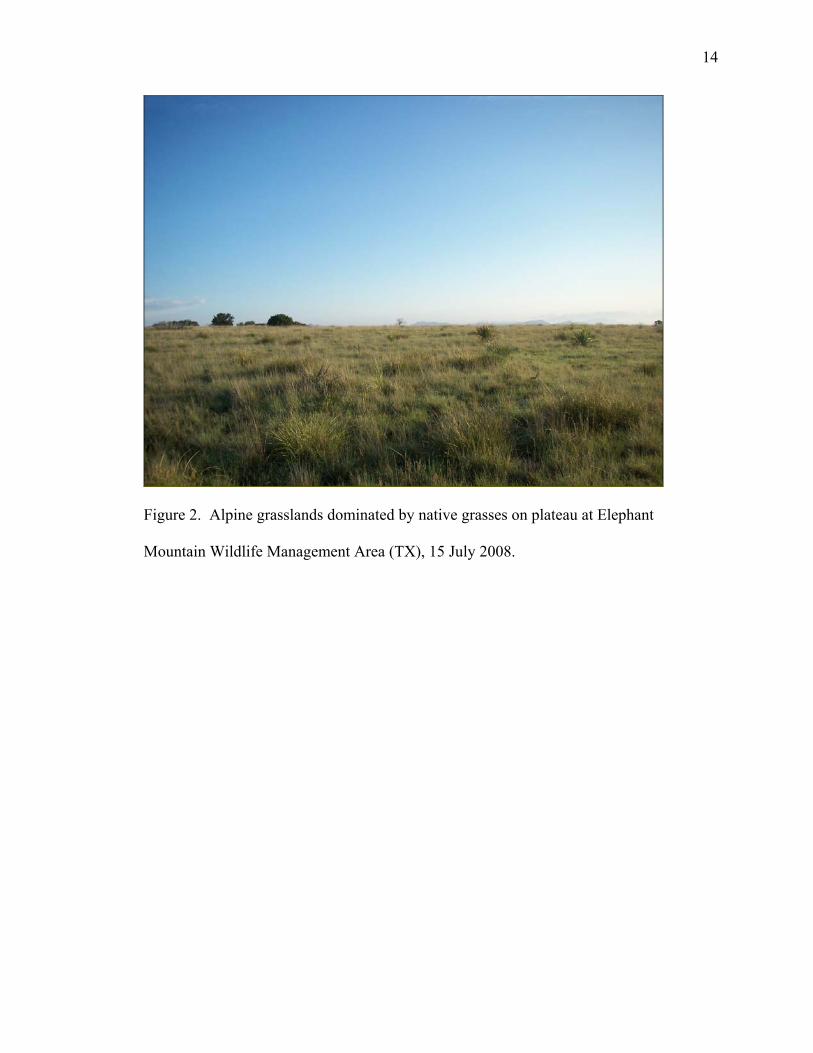
Vegetation on Elephant Mountain WMA consists of alpine grasslands dominated by
native grasses including sideoats grama (Bouteloua curtinpendula), black grama
(Bouteloua eriopoda), tobosa grass (Pleuraphis mutica), and bristlegrass (Setaria spp.)
(Figure 2). Woody vegetation is characterized by sparse patches of small shrubs
including oak (Quercus spp.), mountain laurel (Sophora secundiflora), and fragrant
13
Figure 1. Elephant Mountain Wildlife Management Area (TX) terrain, 18 July 2008.
14
Figure 2. Alpine grasslands dominated by native grasses on plateau at Elephant
Mountain Wildlife Management Area (TX), 15 July 2008.
15
sumac (Rhus trilobata) (note: these are mostly associated with steep slopes, ravines, and
the edges of exposed bedrock and talus) (Hernández et al. 2006b).
The Davis Mountain Preserve (Davis MP) is an 11,500-ha privately owned nature
preserve in Jeff Davis County, Texas (The Nature Conservancy 2006). The Davis MP is
located approximately 40 km north of Fort Davis in the central region of the Davis
Mountains. The Davis Mountains, along with the Guadalupe and Chisos mountains,
form the “sky islands” of the Trans-Pecos ecoregion (Warshal 1995, DeBano and
Ffolliott 2005). The Davis Mountains Preserve contains Mount Livermore, the second
tallest peak in Texas at 2,225 m. Annual precipitation ranges from 28.2–56.9 cm
occurring mainly during the monsoon season (Jun–Sep). Soils are drained, hilly to steep,
loamy, shallow to deep, and non-calcareous (Soil Conservation Service 1977). Dominant
vegetation types are perennial grasslands, evergreen oak, oak-conifer woodlands, and
oak-conifer forests (Figure 3). The Davis MP is comprised of a continuous extensive
habitat for Montezuma quail; whereas, Elephant Mountain WMA is a small island
habitat. Perennial flowing drainages are common with alluvial soils and mountainous
peaks that range in elevation from 1,500–2,200 m (King 2003). The Davis MP has not
been grazed by livestock since its purchase in the early 1990s, but some herbivores
include elk (Cervus elaphus) and deer (Odocoileus spp.). The Davis MP has
reintroduced fire to the Davis Mountains ecosystem to reduce unnatural fuel loads and
catastrophic wildfire threats and to mimic natural ecosystem processes (The Nature
Conservancy 2006).
The Uvalde Route (UVR) included the following counties; Uvalde, Real,
Edwards, and Val Verde. The UVR began outside of Leaky on Ranch Road 337 due
16
Figure 3. Woody and grassland vegetation at Davis Mountains Preserve (TX), 6 August
2007.
17
west to Campwood. It continued north along Ranch Road 55 to Rocksprings where it
joins Ranch Road 337 to Carta Valley. Upon reaching Highway 227, it continued due
south on Highway 227 until reaching Del Rio, Texas (Figure 4). The area surveyed
included counties that are known as sheep-goat-cattle operations (Albers and Gehlbach
1990). The Edwards Plateau is an uplifted and elevated region originally formed from
marine deposits of sandstone, limestone, shales, and dolomites 100 million years ago
during the Cretaceous Period when this region was covered by an ocean (Texas Parks and
Wildlife Department 2007a). The Edward Plateau region was comprised primarily of
grassland savanna with shrubs and low trees along rocky slopes and drainages (Correll
and Johnston 1970; Stanford 1976; Weniger 1988; Hatch, Gandhi, and Brown 1990;
Baccus and Eitniear 2007). Before European settlement, recurrent fires suppressed
woody plants and maintained the open, grassy nature of the landscape on relatively level
ground but not on steeper slopes and canyon walls (Weniger 1988; Baccus and Eitniear
2007). European settlement brought fences, cows, sheep, goats, and control of fire
(Baccus and Eitniear 2007). Livestock continuously grazed in fenced pastures, disrupting
the natural movement patterns of native grazing animals that allowed plants to rest and
recover from grazing (Baccus and Eitniear 2007). When Bailey and Oberholser surveyed
the plateau, most of the area had already been overgrazed by cattle, goats, and sheep, and
most of the grasses had been depleted and replaced by less desirable woody shrubs
(Schmidly 2002). Many of the plants found in the Edwards Plateau include oaks
Weather.―I recorded time of day, temperature, humidity, and wind speed during
each survey. Temperature, humidity and wind speed were measured using a Kestrel 3000
wind meter (Nielsen-Kellerman Co. Boothwyn, PA).
Precipitation data for Elephant Mountain WMA was obtained from the National
Oceanic and Atmospheric Administration (NOAA; http://www.weather.gov/climate
/index.php?wfo=alp) center from the Alpine-Casparis Municipal weather station for July–
August 2007 and June–August 2008. Precipitation data for Davis MP was obtained from
the National Oceanic and Atmospheric Administration (NOAA; http://www.weather.gov/
climate/index.php?wfo=mid) center from Midland/Odessa weather station for Fort Davis
for July–August 2007 and June–August 2008. I partitioned precipitation data into the
same weekly periods that were used for mean weekly calling rates that were previously
defined.
Vegetation Sampling
Microhabitat.—I quantified 2 habitat characteristics (vegetation structure and
food-plant density) at survey points at Elephant Mountain WMA and Davis MP for
subsequent use in resource-selection functions. Variables quantifying vegetation
structure consisted of percent herbaceous coverage (percent litter, forb, grass, and bare
27
ground), vegetation height, and visual obstruction that were measured using a
Daubenmire frame (Bonham et. al 2004), Robel pole (Robel 1969), and vegetation profile
board (Nudds 1977), respectively.
I established 4 30-m transects at each point radiating in the 4 cardinal directions. I
measured vegetation structure at 10 m, 20 m, and 30 m plot along each transect. For
herbaceous coverage, I visually estimated % litter, % forb, % grass, and % bare ground
using a Daubenmire frame. I obtained vegetation height readings using a Robel pole
(Figure 8) from a 4 m distance at 1 m height in each of the 4 cardinal directions (Robel
1969). In addition, I estimated visual obstruction for each of 4-dm strata (0–10, 10–20,
20–30, 30–40) using a profile board following the protocol used for vegetation height (4
m distance, 1 m height, 4 cardinal directions) (Nudds1977). Food-plant density was
determined using a 1- × 1-m frame at 10 m, 20 m, and 30 m plot along each transect. I
recorded the number of individual plants of Allium spp. (Figure 9A–B), Oxalis spp.
(Figure 10), and Cyperus spp. (Figure 11) and calculated food-plant density from this
data.
Macrohabitat.—The macro-scale variables measured at all survey points included
aspect, elevation, slope, and vegetation type. I determined aspect and elevation using
ArcGIS® 9.2. Aspect was given a north, east, south, or west direction depending on the
direction the mountain slope faced. Elevation (m) data was collected from ArcGISTM
Digital Elevation Model (DEM) at a 1 km resolution from the UTM projected coordinate
WGS 1984 UTM ZONE 14. I used the Vegetation types of Texas map as a reference that
was originally made by Texas Parks and Wildlife Department (Figure 12: TPWD 2007c).
28
Figure 8. Example how profile board and Robel pole measurements were conducted at
Davis Mountains Preserve (TX), 5 August 2008.
29
A) B)
Figure 9. A) Allium sp. with flower found at Davis Mountain Preserve (TX), 15 April
2007. B) Allium sp. without flower found at Elephant Mountain Wildlife Management
Area (TX), 28 July 2007.
30
Figure 10. Oxalis sp. found at Davis Mountains Preserve (TX), 4 August 2007.
31
Figure 11. Cyperus sp. found at Davis Mountains Preserve (TX), 29 July 2007.
32
Figure 12. Texas Parks and Wildlife Department Vegetation types of Texas used to
distinguish vegetation types for callback surveys in 2008 survey season (TPWD 2000c).
33
Slope was determined using a Suunto® KB-14 clinometer (Shreveport, LA). To estimate
slope, I first marked my eye level on the profile board, stepped 15 m down slope from the
profile board and measured slope by viewing my eye level through the clinometer. Slope
was collected in degrees. For areas that I did not have access to, slope was obtained
using ArcGISTM 3DTM analyst which is a three-dimensional visualization, topographic
analysis, and surface creation.
My study area encompassed 13 vegetation types. Since the number of survey
points ranged considerably within each vegetation type, I grouped these initial 13
vegetation types into 4 habitat-suitability categories (high, moderate, low, and none) in
order to reduce the number of covariates. Categorization was based on the percentage of
survey points in each habitat type sampled with Montezuma quail detections, information
from prior studies, or observation. High suitability consisted of >50% of survey points
with detections, moderate with at least 26–50% of survey points with detections, low
with 11–25% of survey points with detections, and none with 0–10% of survey points
with detections. For vegetation types not surveyed, I categorized areas as “low” or
“none” depending if areas were sympatric or
allopatric to historical or known Montezuma quail distributions. Sympatric areas were
considered “low” and allopatric areas “none”.
Statistical Analysis
Calling rates and precipitation.―I conducted a Pearson Correlation analysis in
Program SAS on weekly calling rates (calls/survey) and weekly precipitation (mm). I
partitioned weekly calling rates (calls/survey) and precipitation (mm) data into the same
weekly periods that were previously defined. This analysis was conducted for Elephant
34
Mountain WMA and Davis MP separately for each year, pooled across sites for each
year, and pooled across sites and years. Analysis for UVR and DRR was not possible
since the survey points were too spaced out that not any one weather station would have
given a good representation of the precipitation from the area that survey call-back
surveys were conducted.
Occupancy and detection probability.―Prior to conducting any analysis in
Program PRESENCE, I ran a Pearson Correlation Matrix in Program SAS on all of the
variables I had measured throughout my field season. There was a total of 13 micro-scale
habitat variables, 4 weather variables, and 19 macro-scale habitat variables (Table 1). By
using the correlation matrix I was able to reduce the number of variables that were used
in the 3 different analyses ran in Program PRESENCE. Table 1 shows a summary of the
variables measured throughout the field season in 2007 and 2008 with the rationale and
indication as to whether they were removed from my analysis. Using biologically
meaningful variables and a correlation coefficient value of ≥0.60 helped determine which
variables of the set were to remain in the subsequent analysis.
I conducted 3 different analyses in Program PRESENCE. These different
analyses were necessary because not all points had microhabitat data and not all points
were surveyed in both years. Analysis 1 was designed to evaluate the influence of
microhabitat on occupancy and the influence of weather and vegetation height on
probability of detection (Psi [micro-scale], P [weather + vegetation height]). Data for
this analysis was a subset from 2008 (n = 30 survey points from Elephant Mountain
WMA; n = 10 survey points from Davis MP). Not all of 2008 data could be used in this
35
Table 1. Habitat variables measured during survey season 2007 and 2008 at Elephant Mountain Wildlife Management area and Davis
Mountains Preserve with indication of whether they were removed from the analysis.
Scale Initial variable Removed Reason:
Micro-scale Habitat
%Grass cover Has biological importance due to food or for predator concealment.
%Forb cover Has biological importance due to food or for predator concealment.
%Bare ground cover Percent bare ground affects Montezuma quail movements and cover.
%Litter X Percent litter was correlated with %bare ground in 2007, %litter was theleast biologically important.
Allium spp. density X I thought it would be better if I added up the three important plant species (food-plant density) that I measured because Montezuma quail consume all three plantspecies in their diets.
Oxalis spp. density X I thought it would be better if I added up the three important plant species (food-plant density) that I measured because Montezuma quail consume all three plantspecies in their diets.
Cyperus spp. density X I thought it would be better if I added up the three important plant species (food-plant density) that I measured because Montezuma quail consume all three plantspecies in their diets.
Food-plant density Food-plant density was kept because it was the sum of 3 plant species measured (Allium pp., Oxalis spp., and Cyperus spp.) instead of each plant species indivi-dually. It reduced my variables by 3.
36
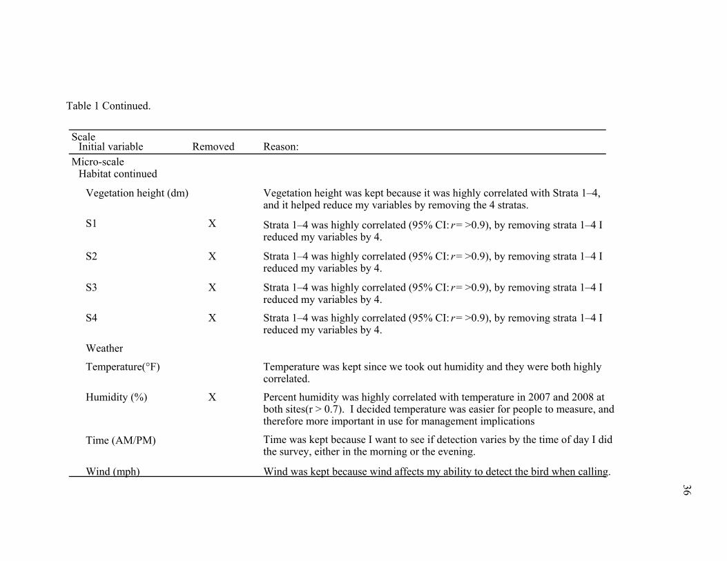
Table 1 Continued.
Scale Initial variable Removed Reason:
Micro-scale Habitat continued
Vegetation height (dm) Vegetation height was kept because it was highly correlated with Strata 1–4, and it helped reduce my variables by removing the 4 stratas.
S1 X Strata 1–4 was highly correlated (95% CI: r = >0.9), by removing strata 1–4 I reduced my variables by 4.
S2 X Strata 1–4 was highly correlated (95% CI: r = >0.9), by removing strata 1–4 I reduced my variables by 4.
S3 X Strata 1–4 was highly correlated (95% CI: r = >0.9), by removing strata 1–4 I reduced my variables by 4.
S4 X Strata 1–4 was highly correlated (95% CI: r = >0.9), by removing strata 1–4 I reduced my variables by 4.
Weather
Temperature(°F) Temperature was kept since we took out humidity and they were both highly correlated.
Humidity (%) X Percent humidity was highly correlated with temperature in 2007 and 2008 at both sites(r > 0.7). I decided temperature was easier for people to measure, and therefore more important in use for management implications
Time (AM/PM) Time was kept because I want to see if detection varies by the time of day I didthe survey, either in the morning or the evening.
Wind (mph) Wind was kept because wind affects my ability to detect the bird when calling.
37
Table 1 Continued.
Scale Initial variable Removed Reason:
Macro-scale
Slope (°) I wanted to see if occupancy varies by the degree of slope.
Elevation (m) I wanted to see if occupancy varies at different elevations.
Aspect (N, E, S, W) X Aspect did not help explain occupancy or probability of detection so I removedit since I thought it was the one with least biological importance. It reduced my covariates by 4.
Vegetation type 13 vegetation types were categorized into 4 different habitat suitability types(high, moderate, low, and none) based on calling rates.
38
analysis because there were some survey points within these study areas for which I did
not have access to (i.e., call-back surveys were conducted from the side of the road) and
therefore no microhabitat data. A priori models for the influence of habitat on occupancy
at the micro-scale were constructed based on the knowledge of needs of Montezuma
quail for food, concealment from predators, and movement (Table 2). A priori models
for probability of detection were built on the knowledge of their calling phenology,
weather, and concealment from predators (Table 3). I modeled occupancy and
probability of detection simultaneously (P. Doherty, Colorado State University, personal
communication). That is, I modeled a particular detection model with each possible
occupancy model.
Analysis 2 represented an additional assessment of the influence of weather and
vegetation height on probability of detection. This analysis used data from 2007
(Elephant Mountain WMA [n = 30 survey points]; Davis MP [n = 30 survey points]). I
modeled occupancy as constant (1) because occupancy rates were almost 1.0 for both
study sites in 2007 indicating that all points were located in optimum habitat. A priori
models for probability of detection were analyzed based on knowledge Montezuma quail
calling phenology, influence of weather, and need for concealment from predators (Table
4).
Analysis 3 was designed to evaluate the influence of macrohabitat variables on
occupancy in order to develop a predictive occupancy map and assess the influence of
weather on probability of detection. Data used for the macrohabitat models were from
Table 2. Analysis 1 a priori occupancy models for Program PRESENCE based on micro-scale habitat characteristics. All model
combinations for analysis are shown.
Variable Model Basis Explanation0 ψ (.) No influence Constant occupancy
1 ψ (food density) Food Presence influenced by primary food plantsψ (grass cover) Concealment (horizontal) Presence influenced by predation vulnerabilityψ (vegetation height) Concealment (vertical) Presence influenced by predation vulnerability
2 ψ (food density + grass cover) Food + Concealment (horizontal)ψ (food density + vegetation height) Food + Concealment (vertical)
3 ψ (food density + grass cover + vegetation height)
40
Table 3. Analysis 1 a priori detection models for Program PRESENCE at a micro-scale based on weather variables and vegetation
height. All model combinations for analysis are shown.
Variable Model Basis Explanation 0 p(.) No influence Constant detection
1 p(survey) Calling phenology Calling varies through season p(time) Calling phenology Calling varies through day p(temperature) Weather Activity varies with heat p(wind) Weather Audibility varies with wind p(vegetation height) Habitat Visual detectability varies with cover
Table 9. Ranking of habitat types into habitat-suitability categoriesa (high, moderate, low, and none) based on the percentage of
survey points with Montezuma quail detections at Elephant Mountain Wildlife Management Area, Davis Mountains Preserve, Uvalde
Route, and Del Rio Route in June–August 2008. (N = Number of survey points, D = Number of survey points with detections, d = %
of survey points with detections [D / N]).
High = Montezuma quail were detected at >50% of survey points; Moderate = survey points that had at least 25–50% detections per habitat type; Low = survey points that had at least 10–25% detection per habitat type; None = survey points that had 0–10% detection per habitat type.
Habitat Type N D d Habitat-suitabilityYucca (Yucca spp.) Ocotillo ( Fouquieria splendens )shrub 12 7 58 HighGray Oak (Quercus spp.)-Pinyon Pine (Pinus cembroides )-Alligator Juniper (Juniperus spp.) Parks / Woods
Table 10. Comparison of habitat variables (mean and standard error) by habitat-suitabilitya type (high, moderate, and low) at Elephant
Mountain Wildlife Management Area (N = 30 survey points) and Davis Mountains Preserve (N = 10 survey points) in June–August
2008.
aHigh = Montezuma quail were detected at >50% of survey points, Moderate = survey points that had at least 25–50% detections per habitat type, Low = survey points that had at least 10–25% detection per habitat type.
compared to the remaining habitat types in 2008 (Table 13). Mean calls/pt was 79–99%
greater in high-suitability habitat compared to the remaining habitat types during 2008
surveys (Table 13).
Occupancy and Probability of Detection
I documented high occupancy at both Elephant Mountain WMA (95% CI: 98–100%)
and Davis MP (95% CI: 94–100%) in 2007. Occupancy rates decreased for both
Elephant Mountain WMA (95% CI: 47–90%) and Davis MP (95% CI: 79–100%) in
2008. I documented a low probability of detection during individual surveys at Elephant
Mountain WMA (95% CI: 30–53%) and Davis MP (95% CI: 30–65%) in 2007.
Probability of detection decreased for both Elephant Mountain WMA (95% CI: 14–28%)
and Davis MP (95% CI: 0–20%) in 2008. These decreases in occupancy and probability
of detection again were expected due to the change in survey points between years.
Based on the probability of detection results for each study site and the formula used in
Program SAS, I determined that surveys would have to be repeated 4–5 times in order to
ensure ≥ 90% probability of detection at a point given a Montezuma quail is present.
Habitat Modeling
I began with 17 a priori variables (13 habitat and 4 weather) deemed biologically
relevant to Montezuma quail prior to modeling occupancy and probability of detection at
the microhabitat scale. I reduced this suite to 8 variables (5 habitat + 3 weather) based on
correlation analysis. This decrease in number of variables reduced the number of
microhabitat model combinations that needed to be run from more than one trillion
models to 4,875. Of these 4,875, I removed an additional 4,651 because I deemed them
biologically irrelevant.
61
Table 13. Mean number of birds calling/point and mean calls/point of Montezuma quail
in different habitat-suitability typesa (High, Moderate, and Low). Habitat suitability
types included surveys conducted in Elephant Mountain Wildlife Management Area (N =
150 surveys), Davis Mountains Preserve (N = 150 surveys) in Jun–Aug 2007 and 2008,
and for Uvalde Road Route (N = 125 surveys), and Del Rio Route (N = 100 surveys) in
June–August 2008.
aHigh = Montezuma quail were detected at >50% of survey points, Moderate = survey points that had at least 25–50% detections per habitat type, Low = survey points that had at least 10–25% detection per habitat type, None = survey points that had 0–10% detection per habitat type.
states/texas/ preserves/art6647.html (Accessed December 2007).
Thompson, W. L. 2004. Sampling rare or elusive species. Island Press, Washington
DC, USA.
Vojta, C.D. 2005. Old dog, new tricks: innovations with presence-absence information.
Journal of Wildlife Management 69:845–848.
Warshall, P. 1995. Southwestern sky island ecosystems. In: E. T. LaRoe, editor. Our
living resources: a report to the nation on the distribution, abundance, and health
of U.S. plants, animals, and ecosystems. United States Department of the
Interior, Washington, D.C.. Pp. 318–322
83
Weniger, D. 1988. Vegetation before 1860. Pages 17–24 in B. Amos and F. R.
Gehlbach, eds., Edwards Plateau vegetation. Waco, Tex.: Baylor University
Press.
84
APPENDICES
85
Appendix 1. Statistical Analysis System formula used to determine the number of field
visits required for a 95% detection probability, based off of the probability of detection
Analysis 3 results.
TITLE ‘Calculation of # of visits required for detection.’; OPTIONS PS=60 LS=90 CENTER FORMDLIM=’ ’; DATA RAWDATA ; P=0.004 ; MAX=0.95 ; ADD = P ; TOTAL = P ; n = 1 ;
in1: ADD = ADD* (1-P) ; n+1; TOTAL = TOTAL + ADD; IF TOTAL < MAX THEN DO ; OUTPUT ; GO TO IN1 ; END ; ELSE STOP ; LABEL P= ‘Detection Probability’ MAX=’Probability Upper Limit’ Total= ‘Overall Detection Probability’ n= ‘# of Visits’; PROC PRINT LABEL ; BY P MAX ; VAR TOTAL ; ID n ; RUN ; QUIT ;
VITA Name: Cristela Gonzalez Sanders Place of birth: Eagle Pass, Texas Parents: San Juana Infante and Pedro Gardea Educational background: M.S., Range and Wildlife Management Texas A&M University–Kingsville B.A., Range and Wildlife Management Texas A&M University-Kingsville Work experience: March 2011–Present:
Rangeland Management Specialist Natural Resources Conservation Service Baird, Texas.
September 2009– February 2011: Rangeland Management Specialist
Natural Resources Conservation Service Lampasas, Texas.
January 2007– present: Graduate Research Assistant, Texas A&M University–Kingsville, Caesar Kleberg Wildlife Research Institute, Kingsville, Texas. May 2005–August 2006: Field Technician, Texas A&M University–Kingsville, Caesar Kleberg Wildlife Research Institute, Kingsville, Texas.