AN EVALUATION OF THE ALTMAN Z-SCORE MODEL IN PREDICTING

CORPORATE BANKRUPTCY FOR CANADIAN PUBLICLY LISTED FIRMS

by

Mohammad Ali Reza Ahmed

ACCA Chartered Member – Association of Chartered Certificate Accountants, 2015

BSc Applied Accounting – Oxford Brookes University, 2009

and

Daksha Govind

BSc Finance (minor law) – University of Mauritius

PROJECT SUBMITTED IN PARTIAL FULFILLMENT OF

THE REQUIREMENTS FOR THE DEGREE OF

MASTER OF SCIENCE IN FINANCE

In the Master of Science in Finance Program

of the

Faculty

of

Business Administration

© Mohammad Ali Reza Ahmed 2018

© Daksha Govind 2018

SIMON FRASER UNIVERSITY

FALL 2018

All rights reserved. However, in accordance with the Copyright Act of Canada, this work

may be reproduced, without authorization, under the conditions for Fair Dealing.

Therefore, limited reproduction of this work for the purposes of private study, research,

criticism, review and news reporting is likely to be in accordance with the law, particularly

if cited appropriately.

ii

Approval

Name: Ahmed, Mohammad Ali Reza & Govind, Daksha

Degree: Master of Science in Finance

Title of Project: An evaluation of the Altman Z score model in predicting

corporate bankruptcy for Canadian publicly listed firms

Supervisory Committee:

___________________________________________

Professor Christina Atanasova

Senior Supervisor

Associate Professor, Finance

___________________________________________

Dr Victor Song

Second Reader

Lecturer, Finance

Date Approved: ___________________________________________

Note (Don’t forget to delete this note before printing): The Approval page must be only one page

long. This is because it MUST be page “ii”, while the Abstract page MUST begin on page “iii”. Finally,

don’t delete this page from your electronic document, if your department’s grad assistant is producing

the “real” approval page for signature. You need to keep the page in your document, so that the

“Approval” heading continues to appear in the Table of Contents.

iii

Abstract

The purpose of this study is to assess the effectiveness of Altman’s Z score in

predicting corporate bankruptcy for Canadian listed companies. First, we estimate

Altman’s original model and test the efficiency of the cut-off region, coefficients and the

variables used. Secondly, we add Cash Flow from Operation (CFO) to Total Liabilities

(TL) ratio as a sixth variable to improve Altman’s (1968) standard Z score model. By

testing and comparing these models using a sample of 70 bankrupt firms against a

population sample of 1,047 non-distressed firms, this study determines which models has

a higher discriminating ability. While Altman’s research focuses on manufacturing

companies, for the purpose of this study, we selected firms from five sectors; energy,

consumer discretionary, consumer staples, industrials and materials. We use Multiple

Discriminant Analysis (MDA) to compare the predictive abilities of these models. Our

results show that the cut-off regions and the coefficients used by Altman should be time-

varying and that our augmented model produces better results, when removing the effects

of outliers.

Keywords: Altman Z score, MDA, Six variable model, RD-CA model, CFO to

Total Liability ratio, Canada, Corporate Bankruptcy, Bankruptcy prediction.

iv

Dedication

I would like to dedicate this thesis equally to my mother Dr. Mahjabeen Sultana

Begum and my wife Shaila Shams who have been immensely supportive of my work. I

would also like to dedicate this work to my father, Dr. Farid Ahmed who has been an

inspiration for me since I was little and naïve. Last but not the least, I would like to dedicate

this work to the hundreds of MSc students to come in the future cohorts – May you find

the same amount of enjoyment that I felt undertaking this thesis and this Master of Finance.

Mohammad Ali Reza Ahmed

I would like to dedicate this thesis to my parents, Parmeelabye Govind and Sanjai

Govind without whom I would not have been able to pursue this Master degree in finance.

I would also like to thank my sisters, Yajna Govind and Bhavna Govind for their

unflinching support.

Daksha Govind

v

Acknowledgements

We would like to thank Professor Christina Atanasova for her continuous support and

mentorship throughout the process of writing this paper.

Without Professor Christina Atanasova’s insightful inspiration, sound guidance and

instruction it would not have been possible to complete this thesis within such a short

period. It has been a tremendously rewarding and cheerful experience working with her.

Further, we would like to thank Dr. Victor Song for his time and commitment to review

this master thesis.

vi

Table of Contents

Approval .......................................................................................................................................... ii

Abstract .......................................................................................................................................... iii

Dedication ....................................................................................................................................... iv

Acknowledgements .......................................................................................................................... v

Table of Contents ............................................................................................................................ vi

List of Figures ............................................................................................................................... vii

List of Tables ................................................................................................................................ viii

Glossary ........................................................................................................................................... ix

1: Introduction ................................................................................................................................ 1

1.1 Purpose of Study and Overview .............................................................................................. 1

1.2 Motivations.............................................................................................................................. 2

1.3 Background ............................................................................................................................. 4

2: Literature Review ...................................................................................................................... 8

3: Methodology ............................................................................................................................. 11

3.1 Data ....................................................................................................................................... 11

3.2 Brief overview of Methodology ............................................................................................ 11

3.3 Periodic analysis of Z-Score ................................................................................................. 12

3.4 Sample Selection of Bankrupt Firms ..................................................................................... 12

3.5 Construction of Non-Bankrupt Strata Sample ....................................................................... 13

3.6 Multiple Discriminant Analysis (MDA) ............................................................................... 13

3.7 MDA result robustness checks .............................................................................................. 14

3.8 Choice of Accounting Ratios ................................................................................................ 16

3.9 Selection between 5 or 6 variables ........................................................................................ 19

3.10 Selection of optimum sample ................................................................................................ 19

3.11 Comparison of the three models ............................................................................................ 20

3.12 Comparison of Altman Z-score to RD-CA model ................................................................ 20

4: Results ....................................................................................................................................... 23

4.1 The changes in Altman Z-Score ............................................................................................ 23

4.2 MDA and comparison of the 5-variable and 6-variable models ........................................... 24

4.3 Initial comparison between the three models ........................................................................ 26

4.4 The RD-CA final model ........................................................................................................ 29

5: Conclusion and Further Studies ............................................................................................. 31

5.1 Conclusion ............................................................................................................................. 31

5.2 Further Studies ...................................................................................................................... 32

Appendices .................................................................................................................................... 34

Bibliography.................................................................................................................................. 36

vii

List of Figures

Figure 1 - Corporate Bankruptcies in Canada 2000-2017 ................................................................ 4

Figure 2 - Assets and Liabilities of Insolvent Businesses in Canada ............................................... 5

Figure 3 - Corporate Insolvency shares by Top Five Sectors ........................................................... 6

Figure 4 - Mean Z Score 2003-2018 .............................................................................................. 23

Figure 5 - Standard Deviation of Z-Score 2003-2018 .................................................................... 23

Figure 6 - Wilks Lambda for the 20 Samples ................................................................................. 24

Figure 7- Variable factor correlations ............................................................................................ 25

Figure 8 - RD-CA model Discriminant Analysis centroids ........................................................... 26

Figure 9 - Frequency Distribution of Altman Z-Score for Canadian Firms ................................... 27

Figure 10 - Frequency Distribution of the J-UK Model for Canadian Firms ................................. 28

Figure 11 - Frequency Dstribution of the RD-CA Model for Canadian Firms ............................. 28

Figure 12- Z Score Frequency Distribution from 2003 to 2017 ..................................................... 34

viii

List of Tables

Table 1 - Statistical method matrix ................................................................................................ 14

Table 2- MDA Robustness check tables......................................................................................... 25

Table 3 - Type I and Type II error on sample ................................................................................ 26

Table 4 - Statistical Summary and comparison of the three models .............................................. 27

Table 5 - Type I and II error comparison RD-CA (pf) vs Altman whole population ..................... 29

Table 6 - Type I and II error comparison RD-CA vs Altman whole population ............................ 29

Table 7 - Wilks' Lambda of 5 variable and 6 variable RD-CA model samples ............................. 35

Table 8 - Statistical Summary of 6-variable models ...................................................................... 35

ix

Glossary

TSE Toronto Stock Exchange

LSE London Stock Exchange

NYSE New York Stock Exchange

AI Artificial Intelligence

NF Non-Failed or Healthy Firms

EBIT Earnings before Interest and Tax

NF Non Failed Firms or Non-Bankrupt Firms or Healthy firms

MT

Algorithm

Mersenne Twister algorithm

Firms The terms Firms and Companies have been used interchangeably in the

following literature

Delete this feature and heading if you are not using a glossary in your thesis.

Critical note: Never delete the section break below !!!!! This break enables the

differential page numbering between the preliminary roman numeral section and the main

body of your document, in Arabic numbering.

If you cannot see the section break line, turn on the “Show/Hide button on your menu

bar.

Do NOT delete this reminder until just before printing final document.

DO delete these paragraphs of instructional text from your final document.

1

1: Introduction

1.1 Purpose of Study and Overview

In the wake of the 2008 financial crisis, corporate bankruptcy has become an issue

of paramount importance. Despite being developed in the 1960s, Altman’s Z score is still

extensively used to predict corporate bankruptcy. While Altman (1968) proved the efficacy

of his model using manufacturing firms during the period from 1946 to 1965, this study

examines how effective his model is in predicting bankruptcy for a sample of Canadian

firms for the period of 1998 to 2017. Our research question also examines whether the

original Z score can be improved upon.

The purpose of this study is firstly to provide an in-depth analysis of this popular

Z-score model in the perspective of the Canadian Publicly listed companies. Secondly, to

extend the original model by adding CFO to Total Debt ratio as the sixth variable, hereafter

referred to as the RD-CA model, and thirdly, to investigate whether the new model created

has a higher bankruptcy predictability than the original model.

To arrive at the RD-CA model, data have been collected over the years 1998 to

2017. This study is broken down into 3 further sections for better understanding and to

assist the reader to delve deeper into the subject matter.

Section 2 provides a literature review that summarizes the important studies in the

field of Z-score and associated improvement studies. The section also undertakes a detailed

analysis of past research material to ascertain the best practices in improving and

2

determining the Z-score variables. It also approaches the different methods used in testing

the precision of Z-scores as a predictor for bankruptcy.

Section 3, Data and Methodology explains in detail the source of Data and how the

Data has been obtained. The section goes further to give a clear overview of the

methodologies used in this study. It starts with the methodologies used to derive the

coefficients of the revised Z-score model along with a revised version of the J-UK model

with an added CFO to Debt ratio. Our revised coefficients and added variable are then used

to derive a new model which has been called RD-CA model.

Section 4 contains the results of the study where all the four models – the original

Altman’s Z-score, the revised Altman’s Z-score, the J-UK model and the RD-CA model

are compared and contrasted.

Finally, Section 5 summarizes and concludes from the results and earlier sections

to give the reader a definitive direction in terms the predictive ability of the RD-CA model

versus Altman’s original Z score.

1.2 Motivations

2018 marks the 50th anniversary of the seminal paper by Edward I Altman, in which

he presented the then revolutionary bankruptcy prediction model, widely known today as

the Altman’s Z-Score (Altman E. I., 1968). In his study, he pioneered the use of Multiple

Discriminant Analysis (MDA) technique to build a bankruptcy prediction model powered

by five financial ratios.

Prior to his paper, bankruptcies were modelled prevalently by univariate ratio

analysis models, such as the classic study conducted by Beaver which established a

3

platform for further multivariate models (Beaver, 1966). Much work has been done since,

on improving the multivariate Altman Z-Score model and usage of Multiple Discriminant

Analysis (MDA) has been rife. However, other technologies such as logistic regression

(Logit) models have been developed in later years, the best known of them being the

Ohlson’s O-Score (Ohlson, 1980). More recently, increasing computing power has seen

the development of a variety of AI techniques such as neural networks, genetic algorithms,

case-based reasoning and recursive partitioning (Richard H.G. Jackson, 2013). Despite the

advent of such newer techniques, the use of Altman’s Z-score has not receded in popularity.

In fact, renowned research and investment management firms such as the Morningstar, to

this day, do not shy away from comparing their much-coveted structural Distance to

Default model to the Z-score to boast their efficacy (Morningstar, Inc., 2009).

Interestingly, even though Altman’s Z-score was based on US firms and subsequent

studies have spanned over all the continents from Africa to Asia, Australia and Europe, it

is evident that in-depth studies to the Canadian Market is comparatively lacking. Recently,

a research was undertaken which incorporated Beaver’s paper and added the use of the

CFO to Total Debt ratio to the original model and tested its efficacy for British publicly

listed companies (Jeehan Almamy, 2016). The paper concluded that the 6th variable in their

“J-UK” model indeed was an improving factor on the Z-score and the companies sampled

were the ones listed in the British stock markets. Such studies have also been conducted

for the US market indeed by Altman himself in 1968, when he tested the efficacy of this

6th variable in 1968, but no such study was recently undertaken for the Canadian stock

market, in spite of the TSE being comparable to the NYSE or the LSE.

4

1.3 Background

Corporate bankruptcy carries costs and negative externalities affecting stakeholders

both within the company and externally. Even though established models such as

Modigliani and Miller (1958) strongly proposed the benefits of debt, many authors have

demonstrated later that the costs of bankruptcy often outweigh the benefits of higher debts

(Myers, 1966). Several papers have since studied the costs of such events and classified

such costs into different categories such as direct, indirect (or “shortfall”) and loss of tax

credits costs (Altman E. I., A Further Empirical Investigation of the Bankruptcy Cost

Question, 1984) (James S. Ang, 1982) or costs borne by different parties (Branch, 2002).

Detailed studies on the costs of bankruptcies have come up with a variety of results such

as the administrative costs being a function of firm size (James S. Ang, 1982) whilst others

have explored the fact that the ratio of bankruptcy costs to firm size falls as firm size

increases (Warner, 1977). Some researchers have even argued that direct bankruptcy costs

do exist but do not dictate the reorganization decisions post eventum (Timothy C G Fisher,

2005). Nonetheless, it is quite evident that, categorisation or not, corporate bankruptcies

do carry costs.

Figure 1 - Corporate Bankruptcies in Canada 2000-2017

1000

3000

5000

7000

9000

11000

2000 2003 2006 2009 2012 2015

No

. of

Ban

kru

ptc

ies

Year

5

Bankruptcy in Canada is also not a new phenomenon. Exploring the past 17 years

of bankruptcy data from 2000-2017, it can be deduced that Canada has been enjoying a

steady 7.23% average annualised fall in corporate bankruptcies since 2000 (

Figure 1) (Office of the Superintendent of Bankruptcy Canada, 2018).

Figure 2 - Assets and Liabilities of Insolvent Businesses in Canada

However, a closer look at the aggregate of “shortfall or deficit” which is the

difference of liabilities from the assets shows that the costs of bankruptcy have increased

drastically between 2007 and 2016 ( Figure 2).

As an example, the number of corporate bankruptcies in Canada in the year of 2007

was 6,293 and the average deficit per business was 916,733 CAD dollars. In contrast, the

number of corporate bankruptcies in 2016 fell by 57% since 2007 to 2,700 but the average

deficit increased 6.5 times to more than 6 million CAD dollars. The net effect was a deficit

increase of 182% over the 9 years or an annualized average increase of 20%. The results

suggest that corporate bankruptcies have become a rarer but much more precarious

phenomenon over the years.

The number of firms going bankrupt has fallen as an overall trend falling almost

12% on an annualized average rate. However, in recent years, a small number of very large

0

6

12

18

2007 2010 2013 2016

CA

D $

Bill

ion

s

Filing Year

Assets ($M) Liabilities ($M) Deficit

6

business insolvency filings have had a disproportionately large effect on the average deficit

of the insolvency filings. For example, in 2016, the average deficit of insolvency filings

was $16 billion which is three times the deficit of the $5.2 billion figure of 2015. The

lowest average deficit was in 2012 standing at $3.6 billion. The deficit is the difference

between the assets and liabilities of a business at the time of bankruptcy filing.

This premise thus sets the stage for us to investigate further into corporate

bankruptcy models to help improve the warning systems set in place to prevent such

calamities.

Further analysis into Canadian corporate bankruptcy data also reveals that over the

years, the construction has consistently been most bankrupt-prone sector while the

accommodation and food services bankruptcies has increased steadily to take the second

place in this infamous list (Office of the Superintendent of Bankruptcy Canada, 2019).

Figure 3 - Corporate Insolvency shares by Top Five Sectors

On the other hand, the sectors of retail trade, manufacturing and transportation and

warehousing have all seen declining trends in such events. These trends also assist in

identifying the sectors for which it is pertinent to carry out prediction model studies.

5%

10%

15%

20%

2007 2010 2013 2016

% S

har

e

Construction ManufacturingRetail Trade Transportation and Warehousing

Accommodation and Food Services

7

The 5 sectors of energy, consumer discretionary, consumer staples, industrials and

materials were specifically chosen since they comprise of almost 50% of the Canadian

GDP while the rest of the sectors comprise a little less than 50% of the total GDP.

Moreover, other sectors such as Financial, health care and information technology have

very low levels of Total Assets compared to revenue, due to the service nature of their

business.

Finally, the Altman model was specifically designed for the non-service sector,

which has aided in the decision of choosing the specific sectors.

8

2: Literature Review

This study is based primarily on three key pieces of literature. The first piece of

literature was related to the detailed foundation of the Altman’s Z-score which came from

his works published in 1983 (Altman E. I., Corporate Financial Distress, 1983) and 2002

(Altman E. I., Bankruptcy,Credit Resik, and High Yield Junk Bonds, 2002). Both of these

references gave detailed explanations into his methodology, results and conclusions. The

second piece of primary literature pertained to the choice of financial ratios. The earliest

research of note and relevancy to this study was conducted by William H. Beaver in 1966

where he utilized a univariate approach by analysing 30 accounting ratios subdivided into

six groups:- Cash-flow ratios, Net-Income Ratios, Debt to Total Asset Ratios, Liquid-Asset

to Total Asset Ratios, Liquid-Asset to Current Debt Ratios and Turnover Ratios (Beaver,

1966). The third piece of literature gave a more contemporary reference to the combination

of Beaver’s work and Altman’s work to add a 6th variable to the original model for UK

listed corporations (Jeehan Almamy, 2016). The author’s in this study referred to their

model as the J-UK model.

The Altman Model can be looked at as a sum of three parts. The first part is the

variables themselves, the second part is the coefficients attached to each variable and the

third part is the cut-off ranges that dictate the judgment on resultant Z-scores. This model

has stayed exactly same since 1968 for the first two parts discussed above. The cut-off

points, the third part, as originally published by Altman as 1.81-2.99 has also not changed

over the years (Altman E. I., Z-Score History & Credit Market Outlook, 2017).

9

One reason for this lack of evolution in the model has been because of its success

in producing excellent results to testing, both for differing industries and for differing

regions. These results have led researchers to believe in the model to great extents. One

study used Z score, as a “fact”— to identify small and medium firm health in Tuxtepec,

Mexico, where 75% were identified as healthy while 25% were either in the grey zone or

alerted as bankrupt (Hernandez, 2018). Similar studies conducted for NIFTY 50 index

(Sanesh, 2016), Industrial Listed companies in Italy (Celli, 2015), insurance companies

listed in the Amman Stock exchange (Al-Manaseer & Al-Oshaibat, 2018) and the

Indonesian listed Banking Industry (Muammar Khaddafi, 2017) illustrated the reliability

of the Altman Model. However, two of the above papers at some point indicated the need

for a revised Z-score range for the specific regions.

This however does not mean that the model has not been challenged. In fact,

previous literature has proved time and again that some or all of the three parts have room

for improvement.

For example, Muminovic in his paper concluded that even though the Z-score

model was prevalent in the Serbian capital market, keeping the model coefficients and

variables the same, while making minor cosmetic accounting changes, produced inaccurate

results- thus indicating the need for a revised model, both in terms of coefficients and in

terms of cut-off ranges (Muminović, 2013).

Thai et. al used the original Altman model to study the predictability of the model

for Malaysian firms. In their study, they found out that the model produced excellent results

for data 5 years prior to bankruptcy with X1 being the highest discriminating variable.

10

However, they also improvised the cut-off scores and used four ranges instead of the

original three (Thai, Goh, Teh, Wong, & Ong, 2014).

The MDA methods used in deriving the model has also been tested. In fact, one of

the few recent Canadian studies on the Altman Z model was conducted in 2017, which

attempted to create a hybrid Forecasted Artificial Neural Network (FANN) model to best

the Altman model (Mohammad Mahbobi, 2017). The study concluded to be successful,

however, it also exposed that artificial neural network (ANN) models and LOGIT models

do not behave better than the Z model.

The use of Discriminant Analysis has been tested multiple times. A study on 33

failed vs 33 NF listed firms in USA, controversially concluded Factor Analysis as a better

alternative to Discriminant Analysis only after ignoring the “grey zones” for both models

(Chi, 2012). Logit models have also been used as alternative methods without comparing

to MDA (Kim & Gu, 2010) and also compared with MDA methods (Affes & Hentati-

Kaffel, 2016) to give contradicting results on superiority of either method.

Finally, the J-UK model that this study endeavors to replicate has used the same

MDA methods but, as discussed before, have made changes to all the three parts, variables,

coefficients and ranges in an effort to make a better model.

Finally, each paper mentioned here has tried to look at one aspect of the model,

which this study has tried to change by examining all three aspects in order to evaluate the

Altman Z-score model.

11

3: Methodology

3.1 Data

A short overview of the steps taken in this study is provided below and explained

in more details in the later sections. All data were obtained from the Bloomberg LP terminal

and missing data was collected from the SEDAR website (SEDAR, 2018).

3.2 Brief overview of Methodology

This section gives a brief description of the steps taken to arrive at the RD-CA

model. The first step was to analyse the Z-scores of each year starting from 2003 to 2017

in view to evaluate the effectiveness of Altman’s original cut-off region. Next, a sample of

Bankrupt firms was collected and only 5 sector specific firms were chosen from the

selection.

The dataset contained 70 bankrupt firms from the 5 sectors. The next step involved

drawing 20 samples of healthy firms from a list of 1,047 companies. The sample of 70

bankrupt firms was then combined with each sample of 70 healthy firms. The MDA was

conducted on 20 samples of 70 healthy firms and 70 bankrupt firms using Altman’s original

5 variables model. We then ran the MDA for another 20 samples of 70 healthy firms and

70 bankrupt firms based on Altman’s 5 variables model plus the sixth CFO to total debt

variable and compared the results of both models. Of the 20 samples, the sample with the

most optimum statistical characteristics was chosen to form the RD-CA model.

The three models original Altman Z-score, J-UK model and the RD-CA model were

examined against the sample of 1074 NF and 70 bankrupt firms for separation and other

statistical characteristics. Finally, recognizing the ineffectiveness of the J-UK model, only

12

the original Altman Z-score model and the RD-CA model were compared to illustrate the

efficacy of the RD-CA model.

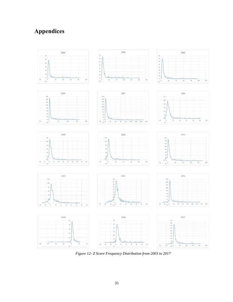
3.3 Periodic analysis of Z-Score

To understand the effectiveness of the Z-score or rather the cut-off points, an

analysis is necessary. This intuition was backed by Altman himself, when he claimed that

the Z-scores have been changing year over year on a Z-score golden jubilee interview event

(Larry Cao, CFA, CFA Institute, 2019). To conduct the analysis, the Z-scores for each year

starting from 2003 to 2017 were compiled and statistical operations were performed to find

the mean, median, standard deviation and kurtosis. The kurtosis was particularly used

instead of skew since the “tailedness” of the data was given more importance due to

outliers. To remove the effects of outliers, the highest 10% and the lowest 10% results were

omitted. Frequency distribution tables were drawn for each list and finally frequency

distribution graphs were produced to illustratively understand the movement of the Z-

scores over the years mentioned above. Error! Reference source not found. in the

Appendix depicts all 15 years.

3.4 Sample Selection of Bankrupt Firms

To obtain the sample of bankrupt firms, data points were collected from the

Bloomberg databases and examined from the years of 1998 to 2017. A query for the field

of companies that filed for bankruptcy for the mentioned years resulted in a total 174 firms.

From the sample of 174 companies, only the companies relevant to the sectors of

energy, consumer discretionary, consumer staples, industrials and materials were taken

into consideration. Moreover, companies which had not started operations, and which did

13

have notable operating activities prior to going bankrupt were disregarded. This left only

70 bankrupt companies in the sample.

3.5 Construction of Non-Bankrupt Strata Sample

To construct the sample of Non-Bankrupt (NF) companies for the random sampling

process, for each sector and each year, firm data was queried on Bloomberg to receive

separate lists of companies. Within these lists, for specific bankrupt firms, the

corresponding prior year of bankruptcy filing was referenced in the collected NF firm lists

and Total Asset sizes were filtered at a range of +/- 50% of the referred bankrupt firm. To

construct its strata of sample firms, the NF list of 2007 was looked at and only firms with

an asset size in the range of 2.75- 6.18 Billion were chosen. Finally, duplicate firms within

the same year and firms that filed for bankruptcy in succeeding years up to 2017 were

omitted.

3.6 Multiple Discriminant Analysis (MDA)

As mentioned earlier, different models before Altman`s 1968 paper used univariate

models to predict corporate failures. The superiority of Altman`s model lay not only in his

multivariate model of prediction but also in the approach that resulted into the multivariate

model. Statistical tools are useful in different contexts and often times using the wrong

statistical methods result in undesirable results. As a rule of thumb, when dependent

variables are qualitative and independent variables are quantitative then discriminant

analysis should be used. The table below gives a guidance on the different methodologies

that should be utilized in different situations.

14

Table 1 - Statistical method matrix

Dependent Variables

Independent

Variables

Quantitative Qualitative

Quantitative Regression Discriminant Analysis/

Binary Regression

Qualitative

Hypothesis Testing/

Regression with dummy

variables

Cross-tab/ Chi-squared

test

For the purpose of this paper, we will use the multiple discriminant analysis (MDA)

to assess the effectiveness of Altman Z score in classifying firms, based on their

characteristics, into bankruptcy and non-bankruptcy. The MDA is a dimension reduction

technique which attempts to draw a cut off line between the two group classifications. It

does so by simultaneously maximizing the distance between the mean of both groups and

minimizing the spread within each group (Brighman & Daves, 2012).

3.7 MDA result robustness checks

To test the robustness of the MDA results, several checks were performed. These

are explained below.

After obtaining the coefficient from the MDA, the first test that we will carry out

is the Wilks’ Lambda which is a measure of means differences which assesses the ability

of the discriminant function in classify firms into bankruptcy and non-bankruptcy. The

lambda value calculated will range between 0 and 1. The higher the lambda value, the

lower is the function’s ability to discriminate.

15

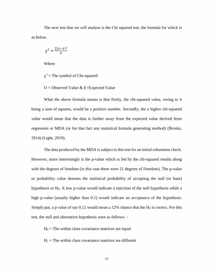
The next test that we will analyse is the Chi squared test, the formula for which is

as below.

𝜒2 =∑(𝑂−𝐸)2

𝐸

Where

2 = The symbol of Chi-squared

O = Observed Value & E=Expected Value

What the above formula means is that firstly, the chi-squared value, owing to it

being a sum of squares, would be a positive number. Secondly, the a higher chi-squared

value would mean that the data is further away from the expected value derived from

regression or MDA (or for that fact any statistical formula generating method) (Brooks,

2014) (Light, 2019).

The data produced by the MDA is subject to this test for an initial robustness check.

However, more interestingly is the p-value which is fed by the chi-squared results along

with the degrees of freedom (in this case there were 21 degrees of Freedom). The p-value

or probability value denotes the statistical probability of accepting the null (or base)

hypothesis or H0. A low p-value would indicate a rejection of the null hypothesis while a

high p-value (usually higher than 0.1) would indicate an acceptance of the hypothesis.

Simply put, a p value of say 0.12 would mean a 12% chance that the H0 is correct. For this

test, the null and alternative hypothesis were as follows: -

H0 = The within class covariance matrices are equal

H1 = The within class covariance matrices are different

16

This test is pertinent since the within class covariance matrices being the same

would mean that the independent variables X1 to X6 perform in identical manners in both

failed and NF firms. This in return would mean that no amount of analysis would produce

discriminating results (Brooks, 2014).

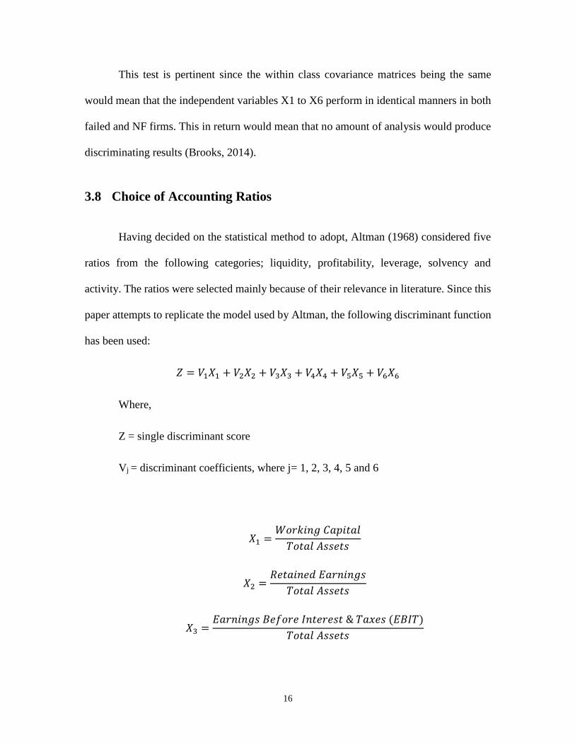
3.8 Choice of Accounting Ratios

Having decided on the statistical method to adopt, Altman (1968) considered five

ratios from the following categories; liquidity, profitability, leverage, solvency and

activity. The ratios were selected mainly because of their relevance in literature. Since this

paper attempts to replicate the model used by Altman, the following discriminant function

has been used:

𝑍 = 𝑉1𝑋1 + 𝑉2𝑋2 + 𝑉3𝑋3 + 𝑉4𝑋4 + 𝑉5𝑋5 + 𝑉6𝑋6

Where,

Z = single discriminant score

Vj = discriminant coefficients, where j= 1, 2, 3, 4, 5 and 6

𝑋1 =𝑊𝑜𝑟𝑘𝑖𝑛𝑔 𝐶𝑎𝑝𝑖𝑡𝑎𝑙

𝑇𝑜𝑡𝑎𝑙 𝐴𝑠𝑠𝑒𝑡𝑠

𝑋2 =𝑅𝑒𝑡𝑎𝑖𝑛𝑒𝑑 𝐸𝑎𝑟𝑛𝑖𝑛𝑔𝑠

𝑇𝑜𝑡𝑎𝑙 𝐴𝑠𝑠𝑒𝑡𝑠

𝑋3 =𝐸𝑎𝑟𝑛𝑖𝑛𝑔𝑠 𝐵𝑒𝑓𝑜𝑟𝑒 𝐼𝑛𝑡𝑒𝑟𝑒𝑠𝑡 & 𝑇𝑎𝑥𝑒𝑠 (𝐸𝐵𝐼𝑇)

𝑇𝑜𝑡𝑎𝑙 𝐴𝑠𝑠𝑒𝑡𝑠

17

𝑋4 =𝑀𝑎𝑟𝑘𝑒𝑡 𝑉𝑎𝑙𝑢𝑒 𝑜𝑓 𝐸𝑞𝑢𝑖𝑡𝑦

𝐵𝑜𝑜𝑘 𝑉𝑎𝑙𝑢𝑒 𝑜𝑓 𝑇𝑜𝑡𝑎𝑙 𝐿𝑖𝑎𝑏𝑖𝑙𝑖𝑡𝑖𝑒𝑠

𝑋5 =𝑆𝑎𝑙𝑒𝑠

𝑇𝑜𝑡𝑎𝑙 𝐴𝑠𝑠𝑒𝑡𝑠

𝑋6 =𝐶𝑎𝑠ℎ 𝐹𝑙𝑜𝑤 𝑓𝑟𝑜𝑚 𝑂𝑝𝑒𝑟𝑎𝑡𝑖𝑜𝑛𝑠 (𝐶𝐹𝑂)

𝑇𝑜𝑡𝑎𝑙 𝐴𝑠𝑠𝑒𝑡𝑠

𝑋1 =𝑊𝑜𝑟𝑘𝑖𝑛𝑔 𝐶𝑎𝑝𝑖𝑡𝑎𝑙

𝑇𝑜𝑡𝑎𝑙 𝐴𝑠𝑠𝑒𝑡𝑠 The denominator consists of the net working capital which is

current assets minus the current liabilities. This ratio indicates the liquidity position of the

firm. It helps stakeholders to understand how much assets are tied up in working capital or

how much fund is available to meet short term financial obligations. A low working capital

to total assets ratio would normally imply financial difficulties experienced by companies.

It could also be interpreted as an early signal to bankruptcy where companies are unable to

pay creditors and suppliers and as a result of which production slows down and sales

contract. (Charles, 1942) is a strong proponent of this ratio and uses it as a leading indicator

for firm cessation.

𝑋2 =𝑅𝑒𝑡𝑎𝑖𝑛𝑒𝑑 𝐸𝑎𝑟𝑛𝑖𝑛𝑔𝑠

𝑇𝑜𝑡𝑎𝑙 𝐴𝑠𝑠𝑒𝑡𝑠 This ratio uses “cumulative profitability over time” to

indicate a firm’s ability to generate income for reinvestment rather than using debt or equity

financing. One of the disadvantages of using this ratio, however, is that it is in favour of

well-established firms at the expense of newly-formed firms. The rationale is that since

newly-established firms have just started operations, they did not have enough time to

generate high earnings. This would result in low retained earnings to total assets which

would imply that those firms are more likely to be classified as bankrupt. The argument

18

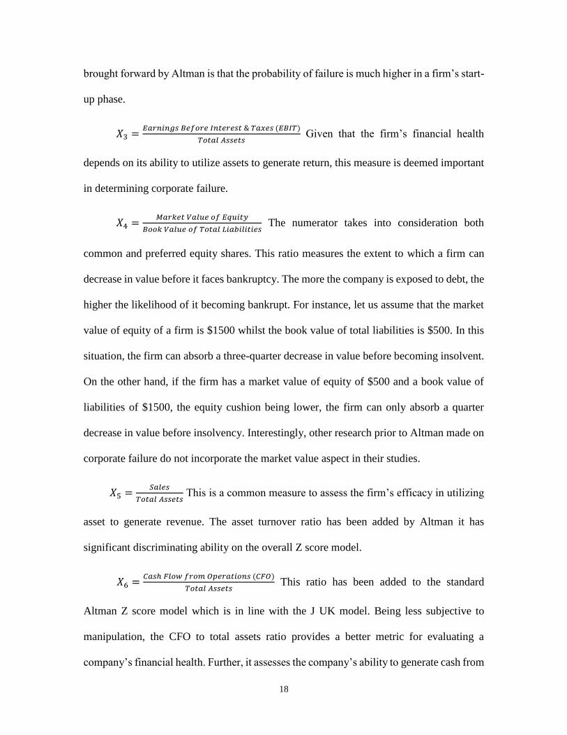
brought forward by Altman is that the probability of failure is much higher in a firm’s start-

up phase.

𝑋3 =𝐸𝑎𝑟𝑛𝑖𝑛𝑔𝑠 𝐵𝑒𝑓𝑜𝑟𝑒 𝐼𝑛𝑡𝑒𝑟𝑒𝑠𝑡 & 𝑇𝑎𝑥𝑒𝑠 (𝐸𝐵𝐼𝑇)

𝑇𝑜𝑡𝑎𝑙 𝐴𝑠𝑠𝑒𝑡𝑠 Given that the firm’s financial health

depends on its ability to utilize assets to generate return, this measure is deemed important

in determining corporate failure.

𝑋4 =𝑀𝑎𝑟𝑘𝑒𝑡 𝑉𝑎𝑙𝑢𝑒 𝑜𝑓 𝐸𝑞𝑢𝑖𝑡𝑦

𝐵𝑜𝑜𝑘 𝑉𝑎𝑙𝑢𝑒 𝑜𝑓 𝑇𝑜𝑡𝑎𝑙 𝐿𝑖𝑎𝑏𝑖𝑙𝑖𝑡𝑖𝑒𝑠 The numerator takes into consideration both

common and preferred equity shares. This ratio measures the extent to which a firm can

decrease in value before it faces bankruptcy. The more the company is exposed to debt, the

higher the likelihood of it becoming bankrupt. For instance, let us assume that the market

value of equity of a firm is $1500 whilst the book value of total liabilities is $500. In this

situation, the firm can absorb a three-quarter decrease in value before becoming insolvent.

On the other hand, if the firm has a market value of equity of $500 and a book value of

liabilities of $1500, the equity cushion being lower, the firm can only absorb a quarter

decrease in value before insolvency. Interestingly, other research prior to Altman made on

corporate failure do not incorporate the market value aspect in their studies.

𝑋5 =𝑆𝑎𝑙𝑒𝑠

𝑇𝑜𝑡𝑎𝑙 𝐴𝑠𝑠𝑒𝑡𝑠 This is a common measure to assess the firm’s efficacy in utilizing

asset to generate revenue. The asset turnover ratio has been added by Altman it has

significant discriminating ability on the overall Z score model.

𝑋6 =𝐶𝑎𝑠ℎ 𝐹𝑙𝑜𝑤 𝑓𝑟𝑜𝑚 𝑂𝑝𝑒𝑟𝑎𝑡𝑖𝑜𝑛𝑠 (𝐶𝐹𝑂)

𝑇𝑜𝑡𝑎𝑙 𝐴𝑠𝑠𝑒𝑡𝑠 This ratio has been added to the standard

Altman Z score model which is in line with the J UK model. Being less subjective to

manipulation, the CFO to total assets ratio provides a better metric for evaluating a

company’s financial health. Further, it assesses the company’s ability to generate cash from

19

its operations as opposed to other sources of funding. The CFO to total assets ratio is hence

considered to be of significant importance predicting corporate bankruptcy.

3.9 Selection between 5 or 6 variables

The MDA described in Section 3.6 was undertaken 40 times. 20 times for the

sample with 6 variables and 20 times with 5 variables. After conducting the checks

presented in Section 3.7, one special check, the Wilk’s lambda, was taken as a measure of

explicability of the models. The Wilk’s lambda was then plotted concurrently for the

respective 5 and 6 variable MDA and compared to derive the final choice of the number of

variables to choose in the final sample.

3.10 Selection of optimum sample

Once the MDA analysis was undertaken for all 20 samples, the samples were then

compared on all the robustness checks explained earlier. On top of these robustness checks,

the formulae generated from the MDA was applied on the whole population of 1074 NF

firms plus the 70 failed firms to produce their respective RD-CA scores. Once these scores

were produced, frequency distribution exercises were undertaken, and frequency

distribution curves were drawn for each of the 1144 Z scores separately for each sample.

Within each sample (produced by the original MDA sample formulae), the RD-CA score

frequency distribution curve of the 70 Failed firms were superimposed on the 1074 NF

score distributions. The peak separations were spotted for each category and the a

“separation of peaks” was calculated as the following formula: -

𝑃𝑒𝑎𝑘 𝑆𝑒𝑝𝑎𝑟𝑎𝑡𝑖𝑜𝑛 = (𝑃𝑒𝑎𝑘 𝑜𝑓 𝑁𝐹 𝐹𝑖𝑟𝑚𝑠) − (𝑃𝑒𝑎𝑘 𝑜𝑓 𝐹𝑎𝑖𝑙𝑒𝑑 𝐹𝑖𝑟𝑚𝑠)

20

Following this exercise, the means, standard deviations and kurtosis of each

category were calculated. A similar separation of means was also calculated. Once these

results were tabulated, (please see index), the manual choice-by-observation was

processed.

For the choice, initially all sample formulae were rejected which either had a

negative peak separation or a negative mean separation. This was done since a negative

separation in either case indicates strongly that the expected RD-CA scores have resulted

in higher values for failed firms when compared with NF firms.

3.11 Comparison of the three models

The tests described in Section 3.8 were also conducted on the Altman Z-score and

the J-UK model by applying the respective formulae to the sample of 1074+70 firms. The

resultant score data were then fed into separate Frequency distribution graphs with similar

superimpositions as 3.9. Similar tests of separation, mean, standard deviation and kurtosis

were also conducted to arrive at the two finalist models between the three models.

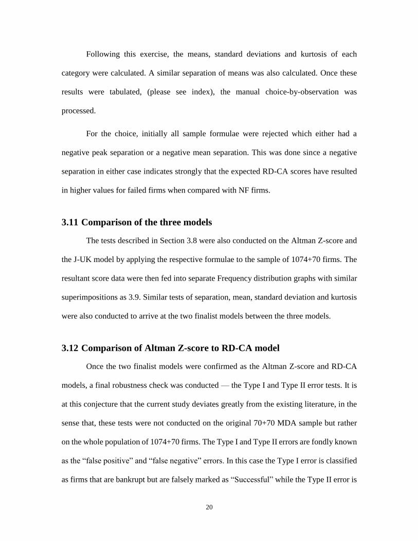
3.12 Comparison of Altman Z-score to RD-CA model

Once the two finalist models were confirmed as the Altman Z-score and RD-CA

models, a final robustness check was conducted — the Type I and Type II error tests. It is

at this conjecture that the current study deviates greatly from the existing literature, in the

sense that, these tests were not conducted on the original 70+70 MDA sample but rather

on the whole population of 1074+70 firms. The Type I and Type II errors are fondly known

as the “false positive” and “false negative” errors. In this case the Type I error is classified

as firms that are bankrupt but are falsely marked as “Successful” while the Type II error is

21

misclassifying the NF firms as bankrupt (Altman E. I., Predicting Corporate Bankruptcy:

The Z Score Model - Empirical Results, 1983). The following table depicts the Type I and

Type II error

Actual Group

Membership

Predicted Group Membership

Bankrupt Non-Bankrupt

Bankrupt Firms Correct Misclassified Type I

NF Firms Misclassified Type II Correct

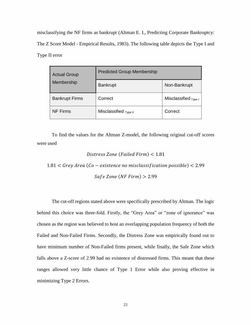
To find the values for the Altman Z-model, the following original cut-off scores

were used

𝐷𝑖𝑠𝑡𝑟𝑒𝑠𝑠 𝑍𝑜𝑛𝑒 (𝐹𝑎𝑖𝑙𝑒𝑑 𝐹𝑖𝑟𝑚) < 1.81

1.81 < 𝐺𝑟𝑒𝑦 𝐴𝑟𝑒𝑎 (𝐶𝑜 − 𝑒𝑥𝑖𝑠𝑡𝑒𝑛𝑐𝑒 𝑛𝑜 𝑚𝑖𝑠𝑐𝑙𝑎𝑠𝑠𝑖𝑓𝑖𝑐𝑎𝑡𝑖𝑜𝑛 𝑝𝑜𝑠𝑠𝑖𝑏𝑙𝑒) < 2.99

𝑆𝑎𝑓𝑒 𝑍𝑜𝑛𝑒 (𝑁𝐹 𝐹𝑖𝑟𝑚) > 2.99

The cut-off regions stated above were specifically prescribed by Altman. The logic

behind this choice was three-fold. Firstly, the “Grey Area” or “zone of ignorance” was

chosen as the region was believed to host an overlapping population frequency of both the

Failed and Non-Failed Firms. Secondly, the Distress Zone was empirically found out to

have minimum number of Non-Failed firms present, while finally, the Safe Zone which

falls above a Z-score of 2.99 had no existence of distressed firms. This meant that these

ranges allowed very little chance of Type 1 Error while also proving effective in

minimizing Type 2 Errors.

22

To find the values of the RD-CA model, a series of 4 ranges were used. The first

range was the centroid range as produced by the MDA. The second was the peak separation

ranges of the failed and NF firms. Since the Failed firms in the 70+70 sample produced 2

peaks a third range was also used in a similar fashion. Lastly, the fourth range was the peak

separation ranges produced by the 1074+70 population. The results were tabulated and

compared to arrive at the conclusion.

23

4: Results

4.1 The changes in Altman Z-Score

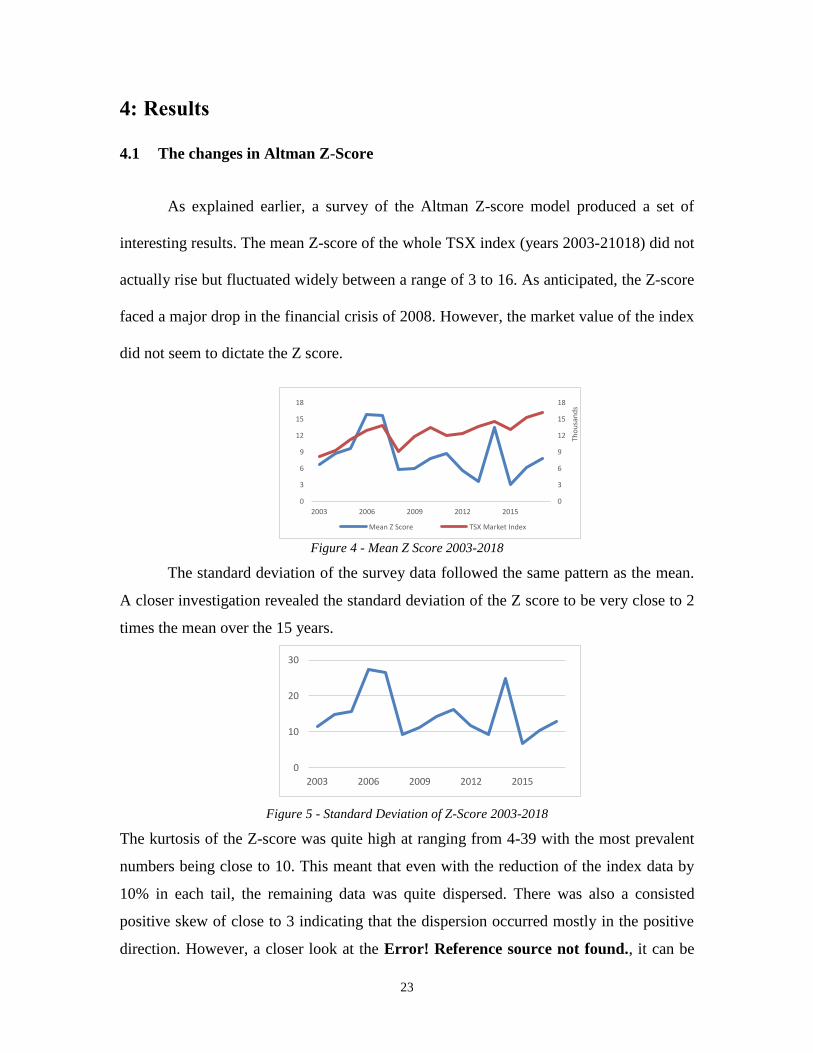
As explained earlier, a survey of the Altman Z-score model produced a set of

interesting results. The mean Z-score of the whole TSX index (years 2003-21018) did not

actually rise but fluctuated widely between a range of 3 to 16. As anticipated, the Z-score

faced a major drop in the financial crisis of 2008. However, the market value of the index

did not seem to dictate the Z score.

Figure 4 - Mean Z Score 2003-2018

The standard deviation of the survey data followed the same pattern as the mean.

A closer investigation revealed the standard deviation of the Z score to be very close to 2

times the mean over the 15 years.

Figure 5 - Standard Deviation of Z-Score 2003-2018

The kurtosis of the Z-score was quite high at ranging from 4-39 with the most prevalent

numbers being close to 10. This meant that even with the reduction of the index data by

10% in each tail, the remaining data was quite dispersed. There was also a consisted

positive skew of close to 3 indicating that the dispersion occurred mostly in the positive

direction. However, a closer look at the Error! Reference source not found., it can be

0

3

6

9

12

15

18

0

3

6

9

12

15

18

2003 2006 2009 2012 2015

Tho

usa

nd

s

Mean Z Score TSX Market Index

0

10

20

30

2003 2006 2009 2012 2015

24

seen that the distribution was at the same time very densely populated around the peak

while the rest of the population was sparsely populated to make the tails longer than usual.

4.2 MDA and comparison of the 5-variable and 6-variable models

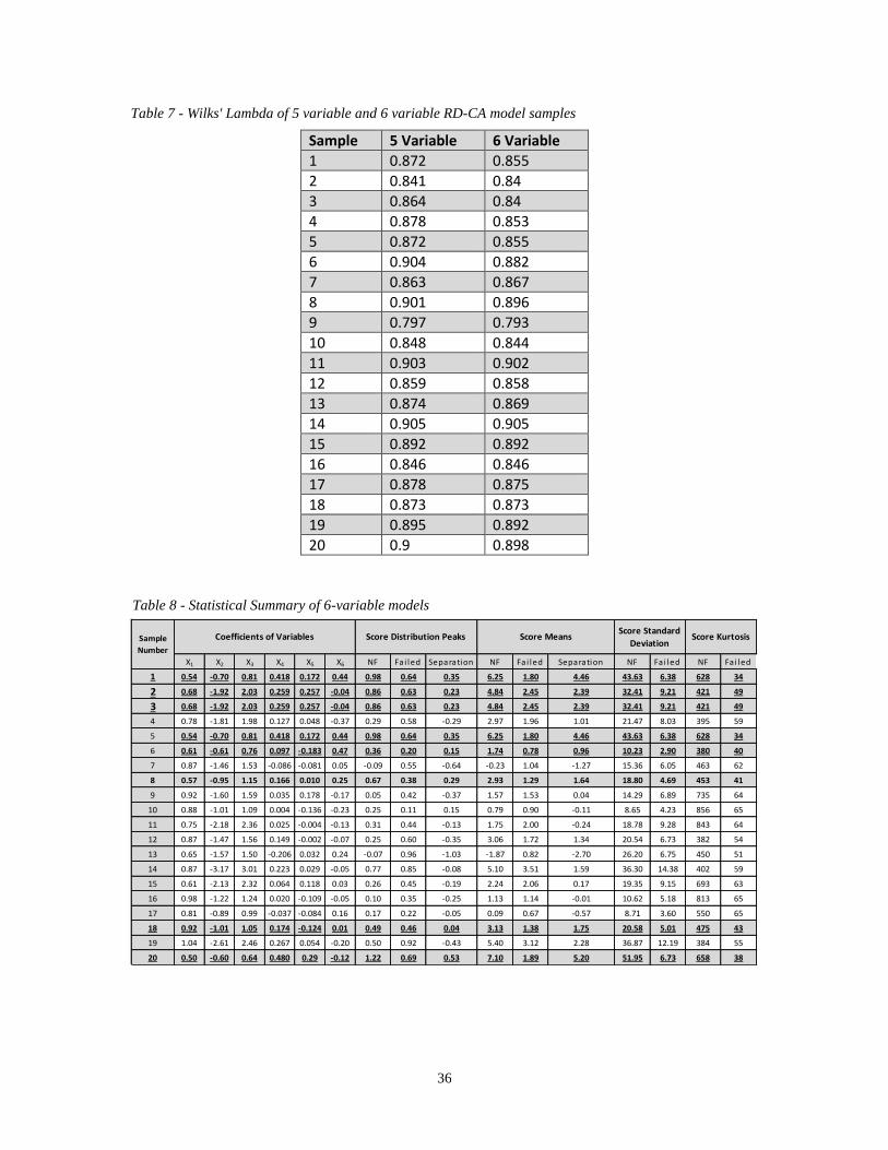
Following the multiple discriminant analysis of the 20 samples, the Wilks’ lambda

of each sample was compared. Table 7 (in the Appendix) illustrates the Wilks’ lambda

across the 20 samples while Error! Reference source not found.6 displays the results

graphically. As depicted from the graph, the 5-variable model lags the 6-variable model by

a small margin and adding a sixth variable to the model decreases the Wilks’ lambda of

respective MDA.

Figure 6 - Wilks Lambda for the 20 Samples

Thus, the resultant 6-variable formulae were taken to derive the resultant optimum

RD-CA model. The statistical summary of the scores from the 1074+70 population are

depicted in Table 7. As a comparison, the Wilks’ lambda of the finally chosen sample

twenty was 0.898 for the 6-variable model when compared with 0.900 for the 5-variable

model.

The resultant RD-CA score distribution peaks, the NF-Failed firm score means,

standard deviations and kurtosis were recorded in Table 8, with the 8 samples that passed

the basic statistical tests highlighted. Sample 20 was chosen from the 8 samples since it

0.79

0.81

0.83

0.85

0.87

0.89

0.91

1 2 3 4 5 6 7 8 9 10 11 12 13 14 15 16 17 18 19 20

6 Variable 5 Variable

25

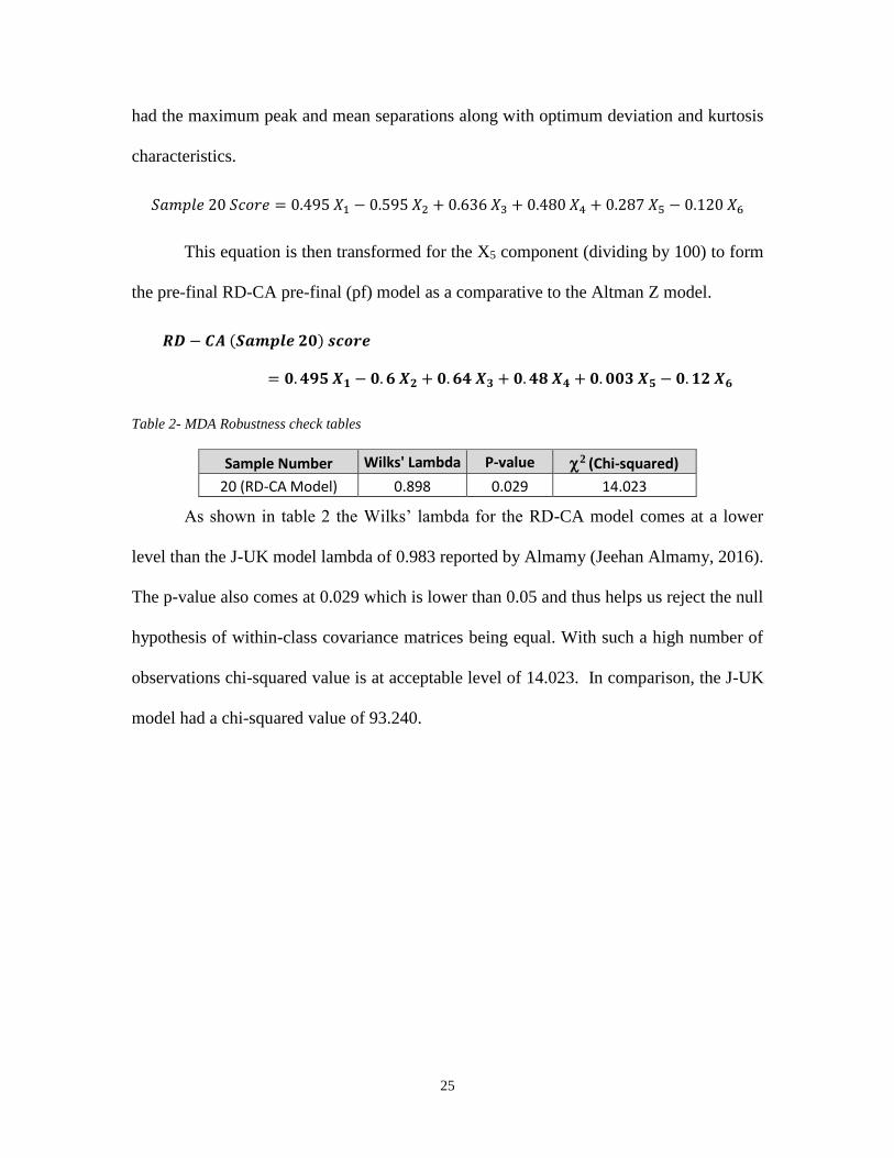
had the maximum peak and mean separations along with optimum deviation and kurtosis

characteristics.

𝑆𝑎𝑚𝑝𝑙𝑒 20 𝑆𝑐𝑜𝑟𝑒 = 0.495 𝑋1 − 0.595 𝑋2 + 0.636 𝑋3 + 0.480 𝑋4 + 0.287 𝑋5 − 0.120 𝑋6

This equation is then transformed for the X5 component (dividing by 100) to form

the pre-final RD-CA pre-final (pf) model as a comparative to the Altman Z model.

𝑹𝑫 − 𝑪𝑨 (𝑺𝒂𝒎𝒑𝒍𝒆 𝟐𝟎) 𝒔𝒄𝒐𝒓𝒆

= 𝟎. 𝟒𝟗𝟓 𝑿𝟏 − 𝟎. 𝟔 𝑿𝟐 + 𝟎. 𝟔𝟒 𝑿𝟑 + 𝟎. 𝟒𝟖 𝑿𝟒 + 𝟎. 𝟎𝟎𝟑 𝑿𝟓 − 𝟎. 𝟏𝟐 𝑿𝟔

Table 2- MDA Robustness check tables

Sample Number Wilks' Lambda P-value 2 (Chi-squared)

20 (RD-CA Model) 0.898 0.029 14.023

As shown in table 2 the Wilks’ lambda for the RD-CA model comes at a lower

level than the J-UK model lambda of 0.983 reported by Almamy (Jeehan Almamy, 2016).

The p-value also comes at 0.029 which is lower than 0.05 and thus helps us reject the null

hypothesis of within-class covariance matrices being equal. With such a high number of

observations chi-squared value is at acceptable level of 14.023. In comparison, the J-UK

model had a chi-squared value of 93.240.

26

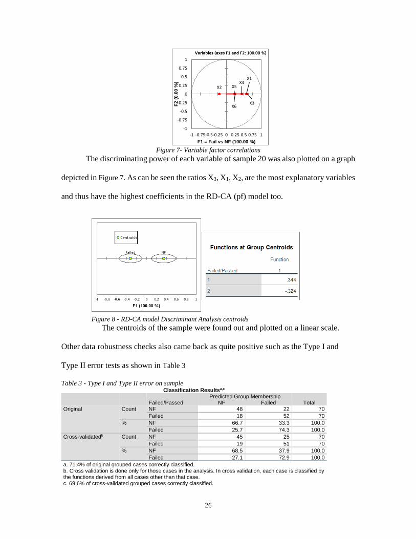
Figure 7- Variable factor correlations

The discriminating power of each variable of sample 20 was also plotted on a graph

depicted in Figure 7. As can be seen the ratios X3, X1, X2, are the most explanatory variables

and thus have the highest coefficients in the RD-CA (pf) model too.

The centroids of the sample were found out and plotted on a linear scale.

Other data robustness checks also came back as quite positive such as the Type I and

Type II error tests as shown in Table 3

Table 3 - Type I and Type II error on sample Classification Resultsa,c

Failed/Passed

Predicted Group Membership Total NF Failed

Original Count NF 48 22 70

Failed 18 52 70

% NF 66.7 33.3 100.0

Failed 25.7 74.3 100.0

Cross-validatedb Count NF 45 25 70

Failed 19 51 70

% NF 68.5 37.9 100.0

Failed 27.1 72.9 100.0

a. 71.4% of original grouped cases correctly classified. b. Cross validation is done only for those cases in the analysis. In cross validation, each case is classified by the functions derived from all cases other than that case. c. 69.6% of cross-validated grouped cases correctly classified.

X1

X2

X3

X4X5

X6

-1

-0.75

-0.5

-0.25

0

0.25

0.5

0.75

1

-1 -0.75-0.5-0.25 0 0.25 0.5 0.75 1

F2 (

0.0

0 %

)

F1 = Fail vs NF (100.00 %)

Variables (axes F1 and F2: 100.00 %)

Figure 8 - RD-CA model Discriminant Analysis centroids

27

As can be seen the model had accuracy of 70% which was quite high when

compared to the J-UK model which subdivided its results to before and after crisis results

and had varying ranges of accuracy between 67% to 81%.

4.3 Initial comparison between the three models

Once the pre-final model was chosen, it was used to receive the scores of all the

1074+70 sample of firms. The same was done for the Altman Z-score and the J-UK model.

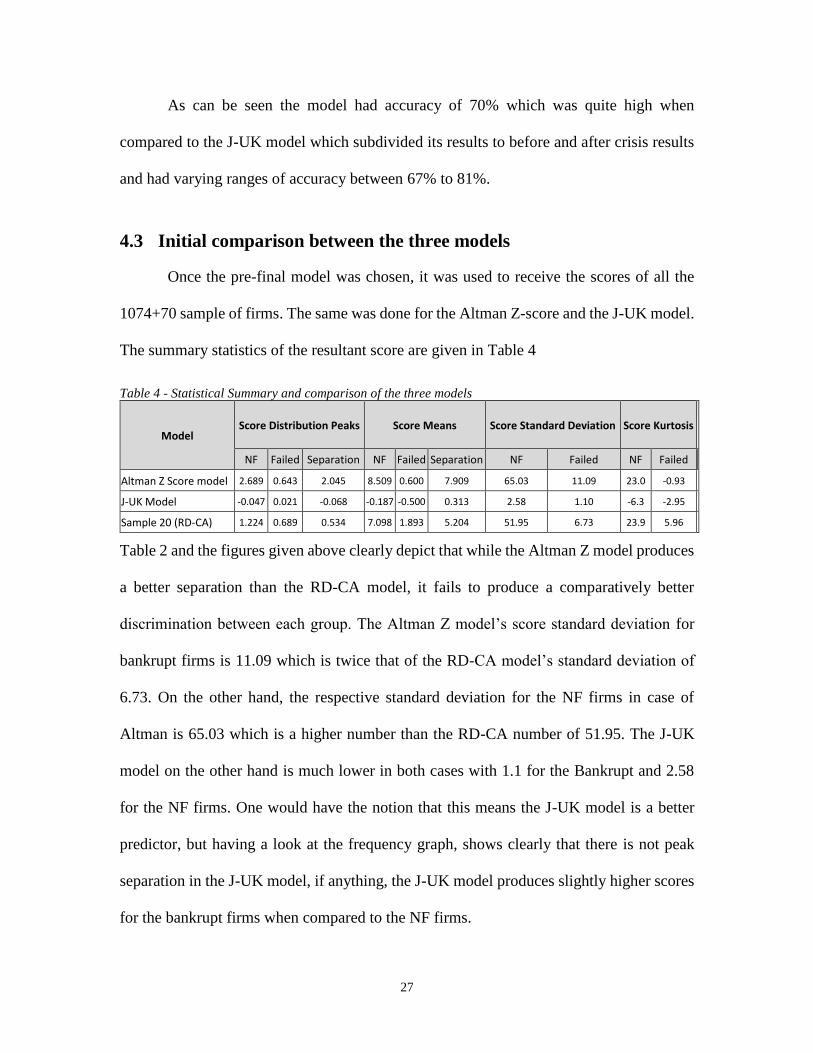
The summary statistics of the resultant score are given in Table 4

Table 4 - Statistical Summary and comparison of the three models

Model Score Distribution Peaks Score Means Score Standard Deviation Score Kurtosis

NF Failed Separation NF Failed Separation NF Failed NF Failed

Altman Z Score model 2.689 0.643 2.045 8.509 0.600 7.909 65.03 11.09 23.0 -0.93

J-UK Model -0.047 0.021 -0.068 -0.187 -0.500 0.313 2.58 1.10 -6.3 -2.95

Sample 20 (RD-CA) 1.224 0.689 0.534 7.098 1.893 5.204 51.95 6.73 23.9 5.96

Table 2 and the figures given above clearly depict that while the Altman Z model produces

a better separation than the RD-CA model, it fails to produce a comparatively better

discrimination between each group. The Altman Z model’s score standard deviation for

bankrupt firms is 11.09 which is twice that of the RD-CA model’s standard deviation of

6.73. On the other hand, the respective standard deviation for the NF firms in case of

Altman is 65.03 which is a higher number than the RD-CA number of 51.95. The J-UK

model on the other hand is much lower in both cases with 1.1 for the Bankrupt and 2.58

for the NF firms. One would have the notion that this means the J-UK model is a better

predictor, but having a look at the frequency graph, shows clearly that there is not peak

separation in the J-UK model, if anything, the J-UK model produces slightly higher scores

for the bankrupt firms when compared to the NF firms.

28

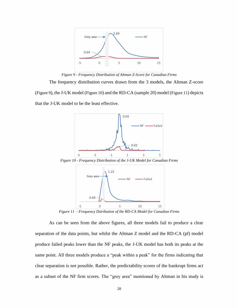
Figure 9 - Frequency Distribution of Altman Z-Score for Canadian Firms

The frequency distribution curves drawn from the 3 models, the Altman Z-score

(Figure 9), the J-UK model (Figure 10) and the RD-CA (sample 20) model (Figure 11) depicts

that the J-UK model to be the least effective.

Figure 10 - Frequency Distribution of the J-UK Model for Canadian Firms

Figure 11 - Frequency Dstribution of the RD-CA Model for Canadian Firms

As can be seen from the above figures, all three models fail to produce a clear

separation of the data points, but whilst the Altman Z model and the RD-CA (pf) model

produce failed peaks lower than the NF peaks, the J-UK model has both its peaks at the

same point. All three models produce a “peak within a peak” for the firms indicating that

clear separation is not possible. Rather, the predictability scores of the bankrupt firms act

as a subset of the NF firm scores. The “grey area” mentioned by Altman in his study is

2.69

0.64

-5 0 5 10 15

NFGrey area

0.03

0.02

-5 -3 -1 1 3 5

NF Failed

1.22

0.69

-5 0 5 10 15

NF FailedGrey area

29

rather the separation “width” within the peaks of each group. This helps us reject the J-UK

model as a viable alternative for the Altman Z model.

It is also quite interesting to see how the RD-CA (pf) model produces peaks with

much less standard deviation which in return results in a “narrower” grey area. This grey

area has been defined as the “zone of ignorance” by Altman (Altman E. I., Establishing a

practical cutoff point, 1983).

In the final step, however it can be seen that the RD-CA (pf) does not fair well

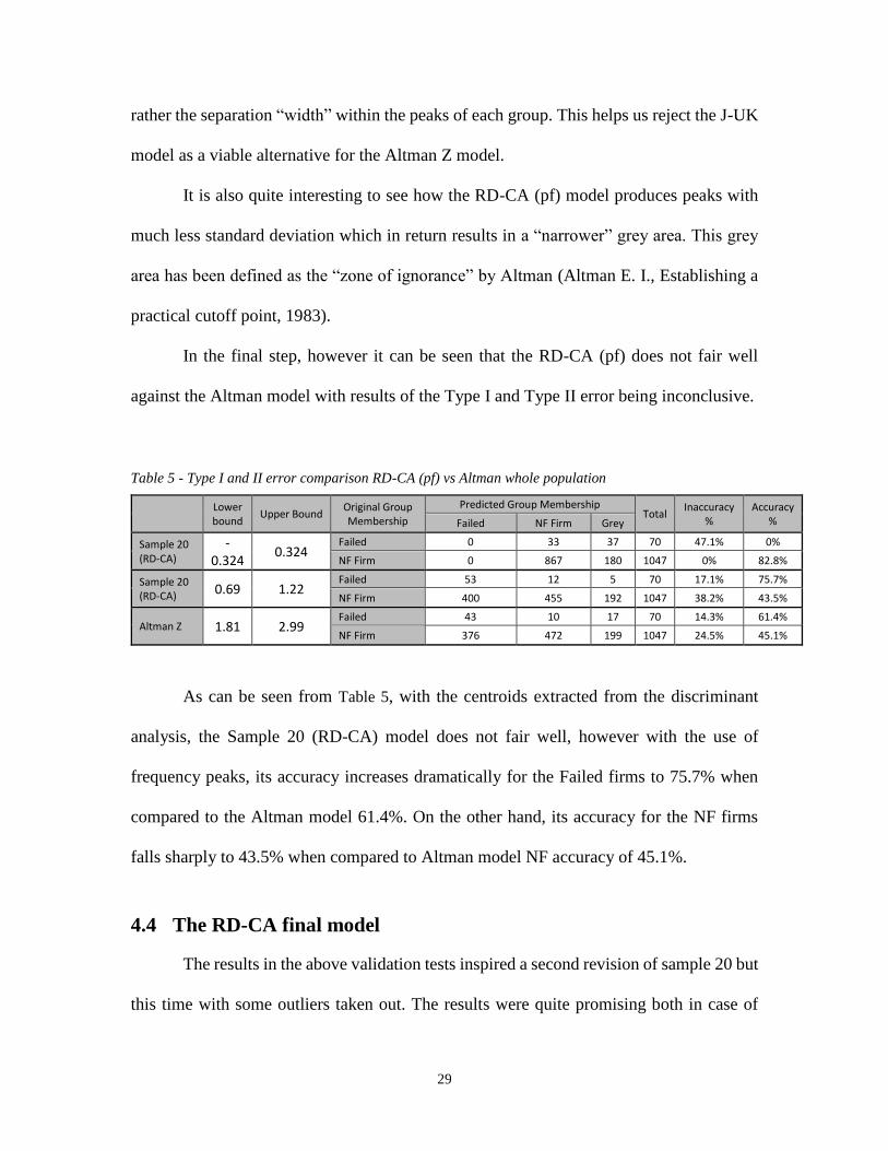
against the Altman model with results of the Type I and Type II error being inconclusive.

Table 5 - Type I and II error comparison RD-CA (pf) vs Altman whole population

Lower bound

Upper Bound Original Group Membership

Predicted Group Membership Total

Inaccuracy %

Accuracy % Failed NF Firm Grey

Sample 20 (RD-CA)

-0.324

0.324 Failed 0 33 37 70 47.1% 0%

NF Firm 0 867 180 1047 0% 82.8%

Sample 20 (RD-CA)

0.69 1.22 Failed 53 12 5 70 17.1% 75.7%

NF Firm 400 455 192 1047 38.2% 43.5%

Altman Z 1.81 2.99 Failed 43 10 17 70 14.3% 61.4%

NF Firm 376 472 199 1047 24.5% 45.1%

As can be seen from Table 5, with the centroids extracted from the discriminant

analysis, the Sample 20 (RD-CA) model does not fair well, however with the use of

frequency peaks, its accuracy increases dramatically for the Failed firms to 75.7% when

compared to the Altman model 61.4%. On the other hand, its accuracy for the NF firms

falls sharply to 43.5% when compared to Altman model NF accuracy of 45.1%.

4.4 The RD-CA final model

The results in the above validation tests inspired a second revision of sample 20 but

this time with some outliers taken out. The results were quite promising both in case of

30

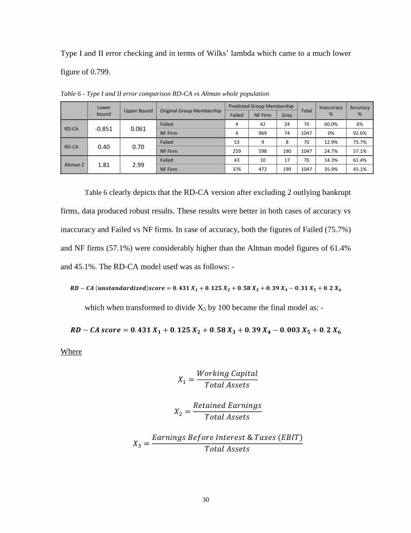
Type I and II error checking and in terms of Wilks’ lambda which came to a much lower

figure of 0.799.

Table 6 - Type I and II error comparison RD-CA vs Altman whole population

Lower bound

Upper Bound Original Group Membership Predicted Group Membership

Total Inaccuracy

% Accuracy

% Failed NF Firm Grey

RD-CA -0.851 0.061 Failed 4 42 24 70 60.0% 6%

NF Firm 4 969 74 1047 0% 92.6%

RD-CA 0.40 0.70 Failed 53 9 8 70 12.9% 75.7%

NF Firm 259 598 190 1047 24.7% 57.1%

Altman Z 1.81 2.99 Failed 43 10 17 70 14.3% 61.4%

NF Firm 376 472 199 1047 35.9% 45.1%

Table 6 clearly depicts that the RD-CA version after excluding 2 outlying bankrupt

firms, data produced robust results. These results were better in both cases of accuracy vs

inaccuracy and Failed vs NF firms. In case of accuracy, both the figures of Failed (75.7%)

and NF firms (57.1%) were considerably higher than the Altman model figures of 61.4%

and 45.1%. The RD-CA model used was as follows: -

𝑹𝑫 − 𝑪𝑨 (𝒖𝒏𝒔𝒕𝒂𝒏𝒅𝒂𝒓𝒅𝒊𝒛𝒆𝒅)𝒔𝒄𝒐𝒓𝒆 = 𝟎. 𝟒𝟑𝟏 𝑿𝟏 + 𝟎. 𝟏𝟐𝟓 𝑿𝟐 + 𝟎. 𝟓𝟖 𝑿𝟑 + 𝟎. 𝟑𝟗 𝑿𝟒 − 𝟎. 𝟑𝟏 𝑿𝟓 + 𝟎. 𝟐 𝑿𝟔

which when transformed to divide X5 by 100 became the final model as: -

𝑹𝑫 − 𝑪𝑨 𝒔𝒄𝒐𝒓𝒆 = 𝟎. 𝟒𝟑𝟏 𝑿𝟏 + 𝟎. 𝟏𝟐𝟓 𝑿𝟐 + 𝟎. 𝟓𝟖 𝑿𝟑 + 𝟎. 𝟑𝟗 𝑿𝟒 − 𝟎. 𝟎𝟎𝟑 𝑿𝟓 + 𝟎. 𝟐 𝑿𝟔

Where

𝑋1 =𝑊𝑜𝑟𝑘𝑖𝑛𝑔 𝐶𝑎𝑝𝑖𝑡𝑎𝑙

𝑇𝑜𝑡𝑎𝑙 𝐴𝑠𝑠𝑒𝑡𝑠

𝑋2 =𝑅𝑒𝑡𝑎𝑖𝑛𝑒𝑑 𝐸𝑎𝑟𝑛𝑖𝑛𝑔𝑠

𝑇𝑜𝑡𝑎𝑙 𝐴𝑠𝑠𝑒𝑡𝑠

𝑋3 =𝐸𝑎𝑟𝑛𝑖𝑛𝑔𝑠 𝐵𝑒𝑓𝑜𝑟𝑒 𝐼𝑛𝑡𝑒𝑟𝑒𝑠𝑡 & 𝑇𝑎𝑥𝑒𝑠 (𝐸𝐵𝐼𝑇)

𝑇𝑜𝑡𝑎𝑙 𝐴𝑠𝑠𝑒𝑡𝑠

31

𝑋4 =𝑀𝑎𝑟𝑘𝑒𝑡 𝑉𝑎𝑙𝑢𝑒 𝑜𝑓 𝐸𝑞𝑢𝑖𝑡𝑦

𝐵𝑜𝑜𝑘 𝑉𝑎𝑙𝑢𝑒 𝑜𝑓 𝑇𝑜𝑡𝑎𝑙 𝐿𝑖𝑎𝑏𝑖𝑙𝑖𝑡𝑖𝑒𝑠

𝑋5 =𝑆𝑎𝑙𝑒𝑠

𝑇𝑜𝑡𝑎𝑙 𝐴𝑠𝑠𝑒𝑡𝑠

𝑋6 =𝐶𝑎𝑠ℎ 𝐹𝑙𝑜𝑤 𝑓𝑟𝑜𝑚 𝑂𝑝𝑒𝑟𝑎𝑡𝑖𝑜𝑛𝑠 (𝐶𝐹𝑂)

𝑇𝑜𝑡𝑎𝑙 𝐴𝑠𝑠𝑒𝑡𝑠

As noted, the value of X5 Sales to Total Assets should have positively affected the RD-CA score

since increasing sales ratios should positively impact a firm’s health.

32

5: Conclusion and Further Studies

5.1 Conclusion

The first conclusion of the study is that the Altman-Z score cut-off range 1.81 < 𝑍 < 2.99

should be updated regularly instead of being used as a fixed range. This is especially true

since the Z score of market index for Canada is a dynamic variable and the numerators and

denominators of the equation do not move in the same proportion from one year to the

next. This results in the prevalent Z-scores (which is in fact a very small range) to move

much higher than the cut-off ranges. This phenomenon in-turn could render the model

useless in its predictability usage. Hence, extreme care must be exercised when assessing

firm health on this metric and performance measurement must be relative to the levels

persistent in the market at the time of assessment.

Secondly, it is observed that adding a sixth variable to the model produces modest

improvements through the robustness checks such as Wilks’ lambda, which could indicate

that a 5 variable model might suffice.

It has also been clarified through this study that, the cut-off scores indeed are not

ranges that should not be viewed as having supreme conclusive power since these ranges

or rather their peaks overlap each other, and no “real” discrimination happens with the use

of MDA.

However, it has been proved beyond doubt that the coefficients of the model do need

to be changed since the discriminating power of the original Altman model seems to be

fading. This change, along with a more dynamic computation of cut-off ranges has

33

produced the RD-CA model which exceptionally outmatches the Altman Z-score model in

precision.

5.2 Further Studies

This study, though detailed, is not free from limitations, of which there are several.

The first remarkable limitation is the use of 5 sectors. Since the advent of the Altman Z-

score, it has been used extensively for all firms across all sectors and has been a staple

name in the financial and investment analysis industry. It is with this notion that the study

was intended. The intention was to produce a generalized scoring model to predict

corporate failure. However, after all the analysis and as already explained in the concluding

remarks, it seems that when it comes to scoring, there is no one-size-fits-all equation.

Therefore, further studies could be conducted with individual sectors to produce a series of

scoring models. It is the belief of the researchers of this study that such methodology would

most definitely produce robust separation in the MDA process.

It is a strong recommendation of the researchers that further research be focused

not only on MDA but also on Factor Analysis since such processed might be more suited

for the categorical classification and separation activities.

Secondly, this study focuses on only six variables. The foundations of this belief

have been Altman himself and Beaver, but numerous other researchers have also had

influence on such decision. This study does not in itself test the efficacy of other ratios to

any extent. It is the belief of the researchers in this study that, due to changing times, the

importance of other financial ratios might very well have increased, and further separate

univariate and multivariate studies could be conducted to produce excellent models.

34

Thirdly, the production of other ratios should also focus on a decreasing reliance

on Total Assets as the dominant denominator in the equation. It is the belief of the

researchers that due to this fact alone, the asset size would drastically affect any prediction

model scores, be it Z-scores or RD-CA scores.

Fourthly, the final RD-CA model provided an unexpected result in having a

negative impact of X5, the sales to total assets ratio. This is in-line with the studies for the

J-UK model and should be further investigated to unearth the reasoning behind such

peculiarities.

Finally, it has been proven through this study that the “centroid theory” does not

hold and the presence of the “peak-within-the-peak” phenomenon of the failed firms within

the non-failed firms. It is thus of great importance that further research should focus on the

frequency distribution curves to derive robust results.

35

Appendices

Figure 12- Z Score Frequency Distribution from 2003 to 2017

36

Table 7 - Wilks' Lambda of 5 variable and 6 variable RD-CA model samples

Sample 5 Variable 6 Variable

1 0.872 0.855

2 0.841 0.84

3 0.864 0.84

4 0.878 0.853

5 0.872 0.855

6 0.904 0.882

7 0.863 0.867

8 0.901 0.896

9 0.797 0.793

10 0.848 0.844

11 0.903 0.902

12 0.859 0.858

13 0.874 0.869

14 0.905 0.905

15 0.892 0.892

16 0.846 0.846

17 0.878 0.875

18 0.873 0.873

19 0.895 0.892

20 0.9 0.898

X1 X2 X3 X4 X5 X6 NF Fai led Separation NF Fai led Separation NF Fai led NF Fai led

1 0.54 -0.70 0.81 0.418 0.172 0.44 0.98 0.64 0.35 6.25 1.80 4.46 43.63 6.38 628 34

2 0.68 -1.92 2.03 0.259 0.257 -0.04 0.86 0.63 0.23 4.84 2.45 2.39 32.41 9.21 421 49

3 0.68 -1.92 2.03 0.259 0.257 -0.04 0.86 0.63 0.23 4.84 2.45 2.39 32.41 9.21 421 49

4 0.78 -1.81 1.98 0.127 0.048 -0.37 0.29 0.58 -0.29 2.97 1.96 1.01 21.47 8.03 395 59

5 0.54 -0.70 0.81 0.418 0.172 0.44 0.98 0.64 0.35 6.25 1.80 4.46 43.63 6.38 628 34

6 0.61 -0.61 0.76 0.097 -0.183 0.47 0.36 0.20 0.15 1.74 0.78 0.96 10.23 2.90 380 40

7 0.87 -1.46 1.53 -0.086 -0.081 0.05 -0.09 0.55 -0.64 -0.23 1.04 -1.27 15.36 6.05 463 62

8 0.57 -0.95 1.15 0.166 0.010 0.25 0.67 0.38 0.29 2.93 1.29 1.64 18.80 4.69 453 41

9 0.92 -1.60 1.59 0.035 0.178 -0.17 0.05 0.42 -0.37 1.57 1.53 0.04 14.29 6.89 735 64

10 0.88 -1.01 1.09 0.004 -0.136 -0.23 0.25 0.11 0.15 0.79 0.90 -0.11 8.65 4.23 856 65

11 0.75 -2.18 2.36 0.025 -0.004 -0.13 0.31 0.44 -0.13 1.75 2.00 -0.24 18.78 9.28 843 64

12 0.87 -1.47 1.56 0.149 -0.002 -0.07 0.25 0.60 -0.35 3.06 1.72 1.34 20.54 6.73 382 54

13 0.65 -1.57 1.50 -0.206 0.032 0.24 -0.07 0.96 -1.03 -1.87 0.82 -2.70 26.20 6.75 450 51

14 0.87 -3.17 3.01 0.223 0.029 -0.05 0.77 0.85 -0.08 5.10 3.51 1.59 36.30 14.38 402 59

15 0.61 -2.13 2.32 0.064 0.118 0.03 0.26 0.45 -0.19 2.24 2.06 0.17 19.35 9.15 693 63

16 0.98 -1.22 1.24 0.020 -0.109 -0.05 0.10 0.35 -0.25 1.13 1.14 -0.01 10.62 5.18 813 65

17 0.81 -0.89 0.99 -0.037 -0.084 0.16 0.17 0.22 -0.05 0.09 0.67 -0.57 8.71 3.60 550 65

18 0.92 -1.01 1.05 0.174 -0.124 0.01 0.49 0.46 0.04 3.13 1.38 1.75 20.58 5.01 475 43

19 1.04 -2.61 2.46 0.267 0.054 -0.20 0.50 0.92 -0.43 5.40 3.12 2.28 36.87 12.19 384 55

20 0.50 -0.60 0.64 0.480 0.29 -0.12 1.22 0.69 0.53 7.10 1.89 5.20 51.95 6.73 658 38

Sample

Number

Score Distribution Peaks Score MeansScore Standard

DeviationScore KurtosisCoefficients of Variables

Table 8 - Statistical Summary of 6-variable models

37

Bibliography

Affes, Z., & Hentati-Kaffel, R. (2016). Predicting US banks bankruptcy: logit versus Canonical

Discriminant analysis. Documents de travail du Centre d’Economie de la Sorbonne, Vol

16. Al-Manaseer, S. R., & Al-Oshaibat, S. D. (2018). Validity of Altman Z-Score Model to Predict

Financial Failure: Evidence From Jordan. International Journal of Economics and

Finance, Vol 10 (08) pp. 181-189.

Altman, E. I. (1968). Financial Ratios, Discriminant Analysis and the Prediction of Corporate

Bankruptcy. The Journal of Finance, Vol. 23, No. 4. (Sep., 1968), pp. 589-609.

Altman, E. I. (1983). Corporate Financial Distress. New York: John Wiley & Sons.

Altman, E. I. (1983). Establishing a practical cutoff point. In E. I. Altman, Corporate Financial

Distress (pp. 119-120). New York: John Wiley & Sons.

Altman, E. I. (1983). Predicting Corporate Bankruptcy: The Z Score Model - Empirical Results.

In E. I. Altman, Corporate Financial Distress (pp. 111-112). Toronto: John Wiley &

Sons.

Altman, E. I. (1984). A Further Empirical Investigation of the Bankruptcy Cost Question. The

Journal of Finance, Vol. 39, No. 4, pp. 1067-1089.

Altman, E. I. (2002). Bankruptcy,Credit Resik, and High Yield Junk Bonds. Massachusets:

Blackwell Publishers Inc. .

Altman, E. I. (2017). Z-Score History & Credit Market Outlook. CTTMA, New Haven Lawn

Club. New Havent, CT: Turnaround Management Association.

Beaver, W. H. (1966). Financial Ratios As Predictors of Failure. Journal of Accounting Research,

Vol. 4, Empirical Research in Accounting: SelectedStudies 1966, pp. 71-111.

Branch, B. (2002). The costs of bankruptcy. International Review of Financial Analysis, Vol 11,

pp. 39-57.

Brighman, E., & Daves, P. (2012). Multiple Discriminant Analysis. In E. Brighman, & P. Daves,

Intermediate Financial Management (pp. Web Extension 25A, 25B). Ohio: South-

Western Cengage Learning.

Brooks, C. (2014). Introductory Econometrics. Cambridge: Cambridge University Press.

Celli, M. (2015). Can Z-Score Model Predict Listed Companies’ Failures in Italy? An Empirical

Test. International Journal of Business and Management, Vol 10 (03) pp. 57-66.

Charles, M. L. (1942). Financing Small Corporations in Five Manufacturing Industries, 1926-36.

New York: National Bureau of Economic Research - Financial Research Program.

Chi, Y. (2012). A Comparative Study of Altman’s Z-score and A Factor Analysis Approaches to

Bankruptcy Predictions. MSc Finance Thesis, Saint Mary's University, pp. 1-43.

Hernandez, C. C. (2018). Small and Medium Size Companies Financial Durability Altman Model

Application. Mediterranean Journal of Social Sciences, Vol 9 No. 2 pp. 9-15.

James S. Ang, J. H. (1982). The Administrative Costs of Corporate Bankruptcy: A Note. The

Journal of Finance, Vol 37 No.1 pp. 219-226.

Jeehan Almamy, J. A. (2016). An evaluation of Altman's Z-score using cash flow ratio to predict

corporate failure amid the recent financial crisis: Evidence from the UK. Journal of

Corporate Finance, Vol 36, pp. 278-285.

Kim, H., & Gu, Z. (2010). A Logistic Regression Analysis for Predicting Bankruptcy in the

Hospitality IndustryHyunjoon KimZheng GuFollow this and additional works

at:https://scholarworks.umass.edu/jhfmThis Refereed Article is brought to you for free

and open access by ScholarWorks. Journal of Hospitality Financial Management, Vol 14

(01) Article 24.

38

Larry Cao, CFA, CFA Institute. (2019, November 25). The Altman Z-Score after 50 Years: Use

and Misuse. Retrieved from CFA Institute:

https://blogs.cfainstitute.org/investor/2016/02/09/the-altman-z-score-after-50-years-use-

and-misuse/

Light, C. (2019, Nov 25). Caitlin Light, Department of Language and Linguistic Science.

Retrieved from University of Pennsylvania:

https://www.ling.upenn.edu/~clight/chisquared.htm

Makoto Matsumoto, T. N. (1998). Mersenne Twister: A 623-Dimensionally Equidistributed

Uniform Pseudo-Random Number Generator. ACM Transactions on Modeling and

Computer Simulation, Vol. 8, No. 1 pp. 3-30.

Microsoft. (2018, November 25). Microsoft Office Support CONCATENATE function. Retrieved

from Office Support Excel: https://support.office.com/en-us/article/concatenate-function-

8f8ae884-2ca8-4f7a-b093-

75d702bea31d?NS=EXCEL&Version=90&SysLcid=1033&UiLcid=1033&AppVer=ZX

L900&HelpId=xlmain11.chm60384&ui=en-US&rs=en-US&ad=US

Mohammad Mahbobi, R. S. (2017). Likelihood of financial distress in Canadian oil andgas

market: An optimized hybrid forecasting approach. Journal of Economic & Financial

Studies, Vol 05 (03) pp. 12-25.

Morningstar, Inc. (2009, July). Comparing Models of Corporate Bankruptcy Prediction: Distance

to Default vs. Z-Score . Chicago, Illinois, USA.

Muammar Khaddafi, F. M. (2017). Analysis Z-score to Predict Bankruptcy in Banks Listed in

Indonesia Stock Exchange. International Journal of Economics and Financial Issues, Vol

7 (03) pp. 326-330.

Muminović, S. (2013). Revaluation and Altman's Z-score- The Case of the Servian Capital

Market. International Journal of Finance and Accounting, 2(1) pp. 13-18.

Myers, A. A. (1966). Problems in the Theory of Optimal Capital Structure. The Journal of

Financial and Quantitative Analysis, Vol. 1, No. 2 pp. 1-35.

Office of the Superintendent of Bankruptcy Canada. (2018, November 25). Insolvency statistics

in Canada (bankruptcies and proposals). Retrieved from Statistics and research - Office

of the Superintendent of Bankruptcy Canada: http://strategis.ic.gc.ca/eic/site/bsf-

osb.nsf/eng/h_br01011.html

Office of the Superintendent of Bankruptcy Canada. (2019, November 25). Ten-Year Insolvency

Trends in Canada 2007-2016. Retrieved from Government of Canada -ISE Development

Canada: https://www.ic.gc.ca/eic/site/bsf-osb.nsf/vwapj/10year-Insolvency-Trends-

Report-EN.pdf/$file/10year-Insolvency-Trends-Report-EN.pdf

Ohlson, J. A. (1980). Financial Ratios and the Probabilistic Prediction of Bankruptcy. Journal of

Accounting Research, Vol. 18, No. 1, pp. 109-131.

Richard H.G. Jackson, A. W. (2013). The performance of insolvency prediction and credit risk

models in the UK: A comparative study. The British Accounting Review, Vol. 45 pp. 183-

202.

Sanesh, C. (2016). The analytical study of Altman Z score on NIFTY 50 Companies. IRA-

International Journal of Management & Social Sciences, Vol 03 Issue 03 pp. 2455-2267.

SEDAR. (2018, November 25). Search Database. Retrieved from System for Electronic

Document Analysis and Retrieval (SEDAR):

https://www.sedar.com/search/search_en.htm

Thai, S., Goh, H., Teh, B., Wong, J., & Ong, T. (2014). A Revisited of Altman Z - Score Model

for Companies Listed in Bursa Malaysia. International Journal of Business and Social

Science, Vol 5 No. 12 pp. 197-207.

Timothy C G Fisher, J. M. (2005). The Irrelevance of Direct Bankruptcy Costs to the Firm's

Financial Reorganization Decision. Journal of Emplirical Legal Studies, Vol 2, Issue 1,

pp. 151-169.

39

Warner, J. B. (1977). Bankruptcy Costs: Some Evidence. The Journal of Finance, Vol 32, No.2,

Papers and Proceedings of the Thirty-Fifth Annual Meeting of the American Finance

Association, Atlantic City, New Jersey pp. 337-347.