Journal of Molecular Structure (Theochem), 221 (1991) 193-211 Elsevier Science Publishers B.V., Amsterdam 193 AN EXAMINATION OF THE SITE-SITE REPRESENTATION OF THE He-H2AND He-N, POTENTIALS* BRIAN HUDSON and JOHN N. MURRELL** School of Chemistry and Molecular Sciences, University of Sussex, Brighton BNl9QJ (Gt. Britain) (Received 15 November 1989) ABSTRACT An analysis has been made of the efficacy of the isotropic site-site model in representing the intermolecular potentials of He-H2 and He-N2 without assuming an analytic form for the site- site interactions. The performance of the method is poor unless the sites are displaced from the nuclei of the diatomic molecules and unless the potential is divided into long- and short-range contributions which are then treated separately. With these levels of flexibility the model is mod- erately successful. INTRODUCTION There are two common approaches to constructing analytical functions for intermolecular potentials. The first is to make a multipolar expansion about the centres of mass of both molecules; the second is to sum the pair interactions between sites distributed among the molecules [ 1,2]. Providing that sufficient terms are taken, and the functions used do not diverge at short distances, both methods should be capable of giving an essentially exact representation of the potential. However, in their truncated forms the performance of both methods may be rather poor. In the bipolar-expansion method the long-range terms are often based on the electric multipole moments of the molecules but these terms may diverge if the distance between the interacting centres is smaller than typical intra- molecular distances. In the site-site method it is usual to adopt isotropic in- teraction terms between the sites placed at the nuclei; this imposes a very con- siderable restriction on the anisotropy of the total potential. The site-site model does seem to be the better approach as the size of the interacting molecules increases, and even for small molecules it has now been *Dedicated to Professor Rudolph Zahradnik **Author to whom correspondence should be addressed. 0166-1280/91/$03.50 0 1991- Elsevier Science Publishers B.V.
AN EXAMINATION OF THE SITE-SITE REPRESENTATION OF THE He-H2AND He-N, POTENTIALS*
BRIAN HUDSON and JOHN N. MURRELL**
School of Chemistry and Molecular Sciences, University of Sussex, Brighton BNl9QJ (Gt. Britain)
(Received 15 November 1989)
ABSTRACT
An analysis has been made of the efficacy of the isotropic site-site model in representing the intermolecular potentials of He-H2 and He-N2 without assuming an analytic form for the site- site interactions. The performance of the method is poor unless the sites are displaced from the nuclei of the diatomic molecules and unless the potential is divided into long- and short-range contributions which are then treated separately. With these levels of flexibility the model is mod- erately successful.
INTRODUCTION
There are two common approaches to constructing analytical functions for intermolecular potentials. The first is to make a multipolar expansion about the centres of mass of both molecules; the second is to sum the pair interactions between sites distributed among the molecules [ 1,2]. Providing that sufficient terms are taken, and the functions used do not diverge at short distances, both methods should be capable of giving an essentially exact representation of the potential. However, in their truncated forms the performance of both methods may be rather poor.
In the bipolar-expansion method the long-range terms are often based on the electric multipole moments of the molecules but these terms may diverge if the distance between the interacting centres is smaller than typical intra- molecular distances. In the site-site method it is usual to adopt isotropic in- teraction terms between the sites placed at the nuclei; this imposes a very con- siderable restriction on the anisotropy of the total potential.
The site-site model does seem to be the better approach as the size of the interacting molecules increases, and even for small molecules it has now been
*Dedicated to Professor Rudolph Zahradnik **Author to whom correspondence should be addressed.
established as the more economical method, at least for the representation of the electrostatic energy [ 3,4]. However, the use of small numbers of sites in- teracting isotropically has proved inadequate in some cases that have been examined in detail. Price [ 51, for example, has shown that for the Nz dimer the use of anisotropic atom-atom potentials is much better than isotropic site- site terms where the position of the sites was optimized.
In testing a model it is normal to optimize parameters in a function to a set of data. The site-site interaction potentials are often represented by simple analytical forms, such as the Lennard-Jones and Born-Mayer functions that have been widely tested for interatomic potentials. The adequacy of the model is then limited by the adequacy of the function. It is, however, possible to test the isotropic site-site model in the simplest case of closed-shell atom-homo- nuclear diatomic interactions without making any assumptions on the form of the site-site function. Moreover, if the model does not work well for this case it is unlikely to be more generally useful. It is for this reason that we examine in this paper the efficiency of the site-site model for the two systems He-H, and He-N,.
THE POTENTIAL SURFACES
The He-H2 potential-energy surface chosen for use in this work was calcu- lated by Senff and Burton [ 61; it is the most extensive and probably the most accurate He-H2 surface yet published. The calculations were carried out using a supermolecule approach with two basis sets, one of 78 and the other of 105 independent functions, denoted as basis A and basis B, respectively. Electron correlation was taken into account using the coupled electron-pair approxi- mation with pair natural orbitals [ 7-91.
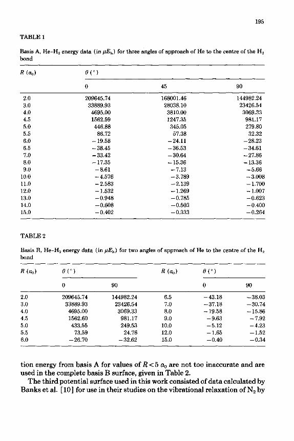
Basis A was used to calculate the potential energy for three angles of ap- proach of He to Hz over a range of R, the distance between the centres of mass, from 2.0 a, to 15.0 a, and an Hz bond length of 1.449 Q. The result was divided into its various components (i.e. the SCF energy and the intra- and inter- correlation energies) and is given in Tables V, VII and VIII of ref. 6. Senff and Burton believe this surface to be slightly inadequate in the van der Waals re- gion due to basis incompleteness affecting the intercorrelation energy; also, the long-range region is dominated by rounding errors and it proved necessary to extrapolate the potential using the formula C (0) /R6, where the values of C for the different angles of approach were deduced from the values of the poten- tial at 9 a,,. The resulting total energy is given in Table 1.
Basis B was used to obtain an improved representation of the intercorrela- tion energy to add to the basis A SCF and intracorrelation energies, these re- sults are given in Table IX of ref. 6. Unfortunately, due to the cost of these calculations, they were carried out only for values of 0 of 0” and 90” and R ranging from 5.0 a, to 15.0 h. It is thought that the values of the intercorrela-
195
TABLE 1
Basis A, He-H2 energy data (in $$,) for three angles of approach of He to the centre of the H, bond
tion energy from basis A for values of R < 5 cq, are not too inaccurate and are used in the complete basis B surface, given in Table 2.
The third potential surface used in this work consisted of data calculated by Banks et al. [lo] for use in their studies on the vibrational relaxation of Nz by
196
collision with He atoms, supplemented with data obtained using the HFDl function of Fuchs et al. [ 111.
The ab initio calculations of Banks et al. were performed using the self- consistent electron-pairs method [ 12,131 with the coupled electron-pair ap- proximation. This method uses wavefunctions which explicitly include all elec- tron configurations which are singly or doubly excited relative to the SCF de- terminant and account for some effects of higher excited configurations implicitly. The basis set consisted of [ 6s4p2d] functions on each nitrogen atom and [5s2p] on the He atom.
The potential was calculated for three different nitrogen bond lengths and two values of 8 over a range of R from 3 a0 to 10 a,. The interaction energies at some selected geometries were recalculated using more extensive basis sets as a test of the surface, this led to the belief that the surface was quite accurate.
For the purposes of this study it was necessary to extend the range of R beyond 10 a,,; this was done by calculating the interaction energy for R > 10 a~ using the HFDl function of McCourt et al. This function consisted of three angle-dependent terms: (1) an exponential with a series of Legendre polyno- mials as an exponent for representing the short-range repulsion; (2 ) a simple series consisting of terms in which R was multiplied by a damping function to represent the induction energy; and (3) a series of dispersion terms each of which is represented by a series based on Legendre polynomials. The repulsion and induction terms were fitted to calculated SCF interaction energies, these were made using a basis set of roughly double-c plus polarization quality for a range of atom-molecule configurations. Since there is little accurate data for the anisotropic dispersion coefficients for the He-N2 interaction, these were
TABLE 3
Comparison of He-N2 energy data (in PI?,,) of McCourt et al. (HFDl) and Banks et al. for two angles of approach of He to the centre of the N, bond
estimated from the highly accurate data available for the N,-N, and He-He interactions using a combination rule.
In their later paper [ 141, McCourt et al. compared this potential-energy function with four other recent He-N, potentials, they conclude that HFDl is probably the most accurate.
An estimate of the percentage difference between the HFDl potential-en- ergy surface at values of R > 10 a, and that which the calculations of Banks et al. would have given in this region, was made by comparing surface energies at selected points for which data were available. These estimates are given in Table 3 and helped to produce the complete composite surface given in Table 4.
DETERMINATION OF THE SITE-SITE INTERACTIONS
The interaction sites were chosen to be the He atom nucleus and two points on the molecular internuclear axis displaced a distance A on either side of the centre of mass. With the molecule and atom in the T configuration it was then possible to write the intermolecular interaction energy as a sum of two iden- tical terms, VA(r), where r is the site-site distance, each representing the in- teraction between the atom and one of the two equivalent sites in the molecule (Fig. 1).
Applying a cubic spline interpolation to the equality V( R ) = 2 VA (r ) , pro- vided tables of VA(r) for selected values of A in the range (approximately) 0.1-1.0 a,, for values of r in the range (again approximately) 2.0-20.0 uo.
If the site-site model is an exact representation of the complete potential then there will be a value of A such that the potential for the linear contigu-
198
ration will be exactly represented by the sum of two terms (see Fig. 2 ) :
V(R) = VA(R- A) + VA@+ A) (1)
Because of the method used to determine VA(r) , this expression can be applied onlywhen (R-A)>r,,and (R+A)<r,,.
A least-squares criterion was used to measure the success of the fit with the difference between the V(R) data and the sum of the site-site functions taken at intervals of 0.05 a, over the range of R in question.
This procedure was first applied to the two He-H, surfaces where an attempt was made to fit the largest possible range of the linear data consistent with the limitations mentioned above. The errors in the fit were virtually identical for both surfaces and are given in Table 5 for the basis-A data. Plots of the most
Fig. 1. The potential V(R) can be written as the sum of two identical site-site functions VA(r).
. R+A
He H H __---
- R-A~tA-A-
Fig. 2. The potential at R is written as the sum of the site-site function VA(r) evaluated at r=R-Aandr=R+A.
TABLE 5
Error (in @,,) in fit tn 0” and 45 ’ basis-A data of the He-H, surface
Fig. 3. He-H, (short-range fit) linear basis-A data fitted with the site-site function.
-50.1. ; 6 i a 5 10 il 12 13 14
Fig. 4. He-H, (long range) linear basis-A data fitted with the site-site function.
200
__
” 3.60
Iis
3.20
2.80 L
2.40
\
2.00
1 .60
0.80
0.40
0.00 _
c I.1
ab initio
A = 0.49 _-__
b = 0.7245 _ _
5. 11: -_-
II P = 0.00
0. III
-4o_.
-45_
Fig. 5. He-H, (short range) 45” basis-A data fitted with the site-site function.
ab initio
--- n = 0.49
- _- __ A = 0.7245
-50 I I 5 G 7 8 9 10 11 12 13 14
R/h
Fig. 6. He-H, (long range) 45” basis-A data fitted with the site-site function.
201
-25
-50
-75 t 4
A = 0.2 lowest broken line
A F 1.2 highest broken line
6 8 I I ,
IO 12 14 16 18
R/a.
Fig. 7. Plots of ab initio data for the T (lower line) and linear configurations (upper line); the increment of A is 0.2 a,.
accurate fit, with A=O.48 a,,, are given in Figs. 3 and 4, again for the basis-A data.
With A=O.49 a, and using the basis-A data the site-site potential can be fitted to the 45” configuration data, this is illustrated in Figs. 5 and 6. The error in this fitting was found to be approximately half that obtained for the linear configuration, rather as one might expect. The error data are given in Table 5. This suggests that any conclusion regarding the reliability of the site- site model reached by comparing the linear- and the T-configuration data will not be contradicted by the data for the 45” configuration.
Figure 7 shows how the fit of the site-site functions to the linear data changes for different values of A and suggests that it might be fruitful to attempt to fit the long- and short-range interaction energies separately. To this end, the T- configuration energy of basis B was separated into a short-range contribution defined as the total energy at values of R < 6.4 a, and a long-range contribution defined as the total interaction energy at values of R > 6.4 %, the distance 6.4
202
TABLE 6
Error in fit to simple short-range data: basis B, He-H, surface
Error in fit to simple long-range data: basis B, He-H2 surface
A (ao)
0.80 0.85 0.86 0.87
Error (@I,)
2.59 1.61 1.55 1.52
A (ao)
0.88 0.89 0.90 1.00
Error (P&J
1.58 1.70 1.87 4.90
uf I
-5
-10
-15
-20 I
Fig. 8. He-H2 (simple long-range function) linear basis-B data fitted with the site-site function.
203
a, being the position of the minimum energy. The limits on the range of R over which it was possible to represent the linear data by the site-site functions are:
Short-range limits x-A>2.0 a,; x+ A~6.4 a, (2)
Long-range limits x-A> 6.4 %; x+ A< 15.0 6
Since the maximum value of A used was 1.0 a~ this meant that it was possible to fit the short-range and the long-range between the values 3.0 a, and 5.4 Q, and 7.4 a, and 14.0 ~0, respectively.
The fitting procedure over these shorter ranges of R was the same as that used over the whole range of R described above. The result was two optimum values of A, a value of 0.48 CQ, for the short-range energy and a value of 0.87 ao for the long-range energy. The results of the fitting procedure are given in Tables 6 and 7. A plot of the short-range result proved in~stin~ishable from Fig. 3 and is not given here, while that of the long-range result is given in Fig. 8.
These calculations were repeated using the basis-A data and similar results were obtained, the two optimum values of A being 0.48 a, and 0.82 ao for the short- and long-range energies, respectively.
A variant on the previous method is to divide the T-configuration data into two by adopting a simple functional form for the short-range part of the po- tential and then define the long-range part as the total energy minus the short- range energy. This procedure constituted the third attempt to tit the linear data with unctions derived from the T-conflation data.
For both sets of He-I-I2 data it was decided that a reasonable short-range potential could be defined as the total potential from 2.0 a, to 4.5 a, extrapo- lated by the simple exponential function A exp ( - bR). The corresponding long- range function incorporates most of the potential well and, to ensure that it approached the axis at 4.5 a, smoothly, it was decided to give it a value of - 5.0 J&& at the point R = 5.0 G. The resulting T-conjuration data for both bases are given in Table 8.
Using the procedure described above, these functions (referred to as the ‘exponential’ short-range and the ‘exponential’ long-range functions) were fit- ted to the appropriate linear data. The short-range functions were fitted over their whole length in the belief that the errors introduced in fitting the poten- tial well and the long-range region would be relatively small.
It proved impossible to fit the minimum in the exponential long-range func- tion to the minimum in the linear data, so it was decided to fit the exponential long-range functions between 7.0 a, and 14.0 a0 and thereby ensure a good fit in the long range at the expense of a bad fit at the well.
The result of this procedure was that the short range linear data from both bases could be fitted best with the relevant exponential short-range site-site functions using A = 0.48 q,; the error data are given in Table 9. The graphs for
204
TABLE 8
Short- and long-range exponential energy data (,a&) for the He-H, surface
the fit were identical to the short range fit shown in Fig. 3 and are not given here.
The long-range linear data were best fitted using site-site functions deter- mined using a value of A of 0.82 CQ for the basis-A data and 0.87 a~ for the basis-
205
TABLE 10
Error in fit to exponential long-range energy data (in &,) for the He-H, surface
B data; the data for these fits are given in Table 10, while their graphs proved virtually identical to those in Fig. 8 and are not given here.
Using the data given in Table 4 an attempt was made to reproduce the linear potential for the He-N, system using its T-configuration data and the site- site model. Exactly the same procedures and methods were adopted for this system as have been described for the He-H, system, except that we used only linear and T-configuration data as there are none for the 45’ configuration.
The site-site function derived from the T-configuration data was first used to reproduce the linear data over the range of R from 4.5 a0 to 20.0 q,. The results, given in Table 11, show the errors in the fit to be a minimum for A= 1.13 u,,. The short- and long-range parts of this fit are shown in Figs. 9 and 10, respectively.
The energy minimum for the T configuration is situated at approximately R = 6.75 o,,; this led to the simple short- and long-range functions being defined as the total potential energy at values of R less than and more than this value, respectively. As the maximum value of A used in this fit was 1.5 %, the limits on the range of R over which the site-site functions could be fitted to the linear data were found to be 4.5-5.25 q, for the short-range function and 8.25-20.5 a, for the long-range function. The first of these ranges is far too narrow for the results of any fitting procedure to be of value, so only the long-range potential
8000
----_ A = 1.13
---_ A = 0.00
4.50 5.00 5.50 6.00 6.50 ;
W a, Fig. 9. He-N2 (long range) linear data fitted in the short-range region.
_ I
ab initlo i \ ----Ar1.13
uf 1 j ; .--- A-O.00
0 I I
-25.
-50. I
-- -75 L
4 , 6 8 10 I 2~ 14 lfi 1%
Fig. 10. He-N2 linear data fitted in the long-range region. wa,
TABLE 12
Error in the fit of the simple long-range data for the He-N, surface
A (4 Error (I&,) A (4 Error (14,)
207
1.30 9.62 1.43 5.73
1.40 5.89 1.44 5.83
1.41 5.76 1.45 6.01
1.42 5.70
----- A = 1.0372
____-- - A = 0.00
409 8.5 10.5 12.5 145 16.5 18.5
R/ a,
Fig. 11. He-N2 (simple long-range function) linear data fitted in the long-range region.
data were fitted. The results of the fit are given in Table 12 and Fig. 11 and show the errors to be a minimum for A= 1.42 a,,.
Finally, the T-configuration potential was divided into a short-range repul- sive potential defined as the total potential between R = 3.0 a, and 4.5 a, and as the simple exponential function, given above, for R > 4.5 uo. The correspond- ing long-range function was defined as the total potential minus this short- range potential in exactly the same way as for the He-H, surfaces. These “ex- ponential” potentials are given in Table 13.
The repulsive potential was fitted over the linear data range 4.5-20.5 a, and produced an optimum value of A of 1.12 a,,. The attractive potential was fitted
208
TABLE 13
Short- and long-range exponential data for the He-N, surface
over a range of R from 8.5 a, to 20.5 %, no attempt being made to fit the region of the potential well. This fit produced an optimum value of A of 1.01 Q. The data are given in Tables 14 and 15, respectively, with almost identical results given in Figs. 10 and 11.
CONCLUSIONS
Irrespective of the range of ii over which the data are fitted, the procedure always produces only one optimum value of A. The errors increase smoothly as values of A increasingly different from the optimum value are used in the fitting; there is no suggestion that these errors may at some point begin to decrease and produce a second minimum in the error curve.
There are two values of A which may a priori be thought of as having special significance: A = 0 and A = half the diatomic bond length. The potential curves for these values are plotted in the appropriate diagrams only where they are significantly different from those curves already shown. In all cases these val- ues produce very poor fits to the linear data and are seen to be of no particular impo~ance.
The site-site potentials resemble slightly stretched versions of the T-config- uration potentials with energy values exactly half the value of the correspond- ing T-configuration energy. The potentials are most similar to the T-configu- ration potential in those regions where that potential has the steepest gradient and the lowest value. In such regions, for example that shown in Fig. 10, the optimum value of A is proportional to the difference in the position on the axis of corresponding features in the T- and linear-configuration data. The opti- mum value of A of the short-range fit for the He-N, interaction (as shown in Fig. 10) is 1.13 Q,, almost exactly the difference in R values between the short- range potentials in the two configurations.
In the case of the He-H, infraction, the short-range region of the T-config- uration potential is considerably less steep than the corresponding region in the He-N, interaction (Fig. 3). When these energies are halved, the site-site potential that results resembles the T-configuration potential moved to smaller values of R. The optimum value of A in this case, at 0.48 a~, is considerably larger than the difference in R between ~orrespon~ng points in the short- range region of the T and linear conjurations, which is approximately 0.2 a~. The facts that the fit of the long-range region requires both a different value of A and a larger value of A than that for the short range are both explained by these observations.
The exponential short-range functions are very similar to the simple short- range functions and the fact that both types require almost the same value of A to provide the best fit is not surprising. The exponential long-range functions are also very similar to the simple long-range functions, although for the He- N, interaction this function is not at all successful.
210
From the considerations mentioned above, it is clear that attempts to fit the region of the potential well will only succeed when the well in the T-configu- ration potential is significantly deeper than the linear-potential well or when the two wells are situated at similar values of R.
Since the fitting procedure consists essentially of pushing the features of the T-configuration potential to higher values of R to match similar features of the linear potential at those R values, it is essential, for the method to work at all, that the features of the linear-configuration potential be at higher R values than those of the T-configuration potential.
Whether or not a single pair of sites with one value of A can be used to reproduce satisfactorily the entire surface will depend on the system in ques- tion. In the case of the two systems considered here, Figs. 3 and 4 suggest that such an approach can provide a very satisfactory result.
The success of the site-site method in this work has implications for the method of representing interactions by an infinite expansion in a series of known functions such as Legendre functions
V(r~R,e)=~V,(r,R)P,(cos8) 1
(3)
where r is the diatomic bond length, R is the distance between the atom and the centre of mass of the diatom and 8 is the angle between r and R. Such expansions tend to be very slowly convergent in the repulsive region of the potential and many terms are required for the fit to be accurate. To evaluate K terms in this expansion it is necessary to calculate sets of points in the (r,R) plane for K different values of 8. However, writing the interaction as a sum of two site-site interactions requires the evaluation of the potential for only two angles
V(r,R$) = V,,(r) + v,,(R,) + VU(&) (4)
Multiplying such a sum by P, (cos 0) and integrating over 8 allows eqn. (3 ) to be obtained to infinite order.
REFERENCES
1 G.C. MaitIand, M. Rigby, E.B. Smith and W.A. Wakeham, Intermolecular Forces Their Or- igin and Determination, CIarendon Press, Oxford, 1981.
2 B. Pullman (Ed. ) , Intermolecular Interactions: From Diatomics to Biopolymers, Wiley, New York, 1978.
3 J.T. Brobjer and J.N. Murrell, Chem. Phys. Lett., 77 (1981) 601. 4 A.J. Stone, Chem. Phys. Lett., 83 (1981) 233. 5 S.L. Price, Mol. Phys., 58 (1986) 651. 6 U.E. Senff and P.G. Burton, J. Phys. Chem., 89 (1985) 797. 7 R. Ahhichs, H. Lischka, V. Staemmler and W. Kutzelnigg, J. Chem. Phys., 62 (1975) 1225. 8 W. Meyer, J. Chem. Phys., 58 (1973) 1017.
211
9 W. Meyer, Int. J. Quantum Chem. Symp., 5 (1971) 59. 10 A.J. Banks, D.C. Clary and H.J. Werner, J. Chem. Phys., 84 (1986) 3788. 11 R.R. Fuchs, F.R.W. McCourt and A.J. Thakkar, J. Phys. Chem., 88 (1984) 2036. 12 J.M. Bowman and S. Leasure, J. Chem. Phys., 66 (1977) 288. 13 R. Schinke and P. McGuire, Chem. Phys., 31 (1978) 391. 14 F.R. McCourt, R.R. Fuchs and A.J. Thakkar, J. Chem. Phys., 80 (1984) 11.