GRIPS GRIPS GRIPS GRIPS Discussion Paper Discussion Paper Discussion Paper Discussion Paper 10 10 10 10-27 The lion’s share. An experimental analysis of polygamy in orthern igeria. By By By By Alistair Munro, Alistair Munro, Alistair Munro, Alistair Munro, Bereket Kebede, Bereket Kebede, Bereket Kebede, Bereket Kebede, Marcela Tarazona Marcela Tarazona Marcela Tarazona Marcela Tarazona-Gomez Gomez Gomez Gomez, and Arjan Verschoor and Arjan Verschoor and Arjan Verschoor and Arjan Verschoor Dec Dec Dec Dec 2010 2010 2010 2010 National Graduate Institute for Policy Studies 7-22-1 Roppongi, Minato-ku, Tokyo, Japan 106-8677
Transcript
GRIPS GRIPS GRIPS GRIPS Discussion PaperDiscussion PaperDiscussion PaperDiscussion Paper 10101010----22227777
The lion’s share.
An experimental analysis of polygamy in �orthern �igeria.
ByByByBy
Alistair Munro,Alistair Munro,Alistair Munro,Alistair Munro, Bereket Kebede,Bereket Kebede,Bereket Kebede,Bereket Kebede,
Across many countries around the world, polygamy is a familiar and apparently robust social institution. Its
most typical form is polygyny, where a husband has two or more wives and in this form it is found commonly
in more than 50 countries world-wide.i Though widespread and seemingly integral to the culture of many
societies, the empirical investigation of polygyny has attracted very little attention from economists. In this
paper we add to the small pool of data, by reporting an experiment with polygynous couples in the northern
Nigerian state of Kano. Given the lack of data on economic behaviour amongst polygynous families, we
concentrate on some simple questions. As with monogamous families, the most straightforward questions to
consider with polygyny are household efficiency and intra-household allocation. Are monogamous
households more efficient than polygamous? In polygynous households, which wife receives the greater
share of incomes? How are resources allocated? These questions provide a starting point for our design
which employs two versions of a one-shot voluntary contribution game: one with a fixed rule of allocating the
communal pool and one in which the husband must make the allocation. The experiment is part of a much
wider programme that investigates patterns of conjugality in several countries. As such it runs in parallel with
near identical experiments on monogamous couples in the same location. In addition we run a follow-up
household survey 1-2 months later, in which wives and husbands are interviewed. In this way we tie our
experimental results to more traditional forms of household data
To offer a quick preview of our results, broadly speaking we find that both types of households in our sample
are equally inefficient in their decisions. In terms of payoffs, senior wives in polygyny fare no worse that
wives in monogamous households, but polygynous husbands do better than their monogamous counterparts.
Most clearly, second wives are disadvantaged compared to their co-spouses when men control the allocation
of resources.
Background.
* This study forms part of “The Intra-Household allocations of resources: Cross-Cultural Tests, Methodological Innovations and Policy Implications”, a project jointly funded by the UK’s ESRC and DFID (RES-167-25-0251). As such the work has benefited greatly at all stages from the expertise and close cooperation of the other members of the team, Cecile Jackson and Nitya Rao. We are also grateful for financial support from the JSPS-funded Global COE “The Transferability of East Asian Development Strategies and State Building”, and for helpful comments received from Takashi Yamano, Yukichi Mano, seminar participants at FASID, Tokyo, Economic Science Association meeting, Melbourne, 2010 and the World Bank. We are especially thankful to the hard-working efforts of our local team, led by Kabiru Bello and Dr. Habu under the guidance of Dr Wakili, the director of the Centre for Democratic Research and Training in Kano.
- 4 -
Table 1 provides some summary statistics about the incidence of polygyny in sub-Saharan Africa - the part of
the world where incidence is highest - over the last 25 years. The percentages of women in polygynous
marriages vary significantly across countries, but are generally higher in the west of Africa. In several
countries, over one third of married women share their husband with one or more wives and while the
percentage doing so has declined over the period, the trend is gentle in most countries and absent in some.
Table 1. Polygyny in sub-Saharan Africaii
% Wives with one or more co-wives
Country Year Country Year
Benin 1996 2001 2006 Mali 1987 2001 2006
49.4 45.4 42.6 45 42.4 39.2
Burkina Faso 1993 1998-99 2003 Mauretania 2001
50.9 54.6 48.4 11.2
Burundi 1987 Mozambique 1997 2003
11.6 27.3 24.2
Cameroon 1991 1998 2004 Namibia 1992 2000 2005
38.2 32.7 30 24.2 12.4 5.5
Chad 1998 2003 Niger 1992 2001 2006
39.1 39 36 37.6 35.7
Cote d'Ivoire 1994 1998 Nigeria 1990 2003 2008
36.4 34.8 40.8 35.7 32.7
Eritrea 1995 2002 Rwanda 1992 1999 2005
6.9 9.3 14.2 12.1 11
Ethiopia 2000 Senegal 1987 1997 2005
13.6 46.5 46 39.5
Gabon 2000 Sierra Leone 2008
21.1 37.3
Ghana 1988 2000 2008 South Africa 1998
32.6 22.5 18.6 6.8
Guinea 1999 2005 Sudan 1989
53.3 53 20.1
Kenya 1988 2003 2008 Swaziland 2007
23.4 16.4 13.3 18.3
Liberia 1986 2007 Tanzania 1992 1997
38 16.3 26.9 28
Madagascar 1992 2003 2007 Togo 1988 1998
5.9 3.1 3.1 52.3 42.8
Malawi 1992 2000 Uganda 1988 2001 2006
20.4 17 34.1 32.2 28.1
Zambia 1992 2001 2007
17.6 15.8 14.4
Source DHS surveys various years. The data includes the most recent and the earliest data for each country.
Nigeria is therefore one of a significant number of countries where polygyny is common and apparently
stable in the sense that it has shown but a slow and erratic tendency to decline in the modern era. According
to the 2008 Demographic and Health Survey, iii
41.9% of married women in the largely Muslim North-west
region of Nigeria (where our study is located) reported having one or more co-wives. Conversely, 27.1% of
married husbands reported two or more wives in the same region. For husbands, this compares to 24.2%
reported for same region in a 1999 survey and a national average of 18.7% in 2008. For wives in north-west
- 5 -
Nigeria, 37.2% reported one or more co-wives in 1999, and 32.7% nationally report one or more co-wives in
2008. Polygyny is more common in rural areas by about six percentage points, more common amongst
individuals with lower education levels and common at all wealth levels. In the vast majority of polygynous
marriages, 2 wives are married to one man, but 2.6% of married men in 2008 reported having 3 or more
wives.
We focus on the Hausa people, the largest ethnic group in the north of Nigeria who also live in large
numbers in neighbouring countries such as Niger. Hausa are Muslims and practice female seclusion as a
cultural norm for married women (Hill, 1969). Married women do not generally go out in daylight except for
occasions such as marriage ceremonies or to seek medical help (Calloway, 1984, Robson 2004). Among the
Hausa, the reality of female seclusion varies with the nature of the settlement and the prosperity of the family.
In general, it is more complete in urban areas and amongst higher income families (Calloway, 1984). In
dispersed settlements away from the main towns there can be relatively little seclusion. Although seclusion
limits their physical mobility, women have a significant degree of economic autonomy. They engage in
various small scale enterprises and many are highly active producers and traders of craft and food products.
In this regard, children act as intermediaries with girls to the fore, hawking goods, passing messages and
learning the skills of the marketplace. In Robson, 2004, girls spend twice as much time per week on trading
as they do on domestic work and four times as much time as boys do.
What money wives earn is usually for themselves, accounts are kept strictly separately from their partners
and spent according to their own priorities. “In Kano [the main city of the region], a woman's trade is so
individual that a husband will actually buy prepared food from his wife for his meals.” Calloway, 1984, p. 440.
Meanwhile men are responsible for providing normal consumption goods, housing and investing in
agriculture. Divorce is relatively common and frequently initiated by women (in 86% of cases according to
Solivetti, 1994). Jackson, 1993, reports a lifetime average of 2.3 marriages per woman amongst Hausa,
while Calloway concludes that around 50% of women will at some stage in their lives go through the process
of divorce, emphasizing that remarriage is the overwhelming norm for pre-menopausal women and occurs
rapidly because most women who would otherwise face social isolation. Overwhelmingly in our survey, both
men and women state that, upon divorce men and women typically retain their own property, including land,
livestock, tools, cash and housing. Older boys and girls usually go with fathers, while younger children,
especially girls, are more likely to go with mothers.
Population density is relatively high and most farming is intensive. Crops include wheat, rice, millet, sorghum,
maize, cowpeas and groundnuts. There is some livestock farming and vegetables. The practice of seclusion
means that while they engage heavily in agricultural processing activities for their own profit, married Hausa
women play little role in cultivation, which is carried out largely by men with the aid of children (Hill, 1969;
Jackson, 1985).iv Hausa is a patrilineal society and one patrilocal extended family normally occupies a single
compound with separate dwellings for each wife.
- 6 -
Theory Background.
Although polygyny is common, interest in it from an economic perspective has been intermittent and
economic theories about it are correspondingly rare. In Becker’s pioneering, discussion, variation in male
productivity is given as one possible reason for polygyny. Total output maybe higher when more than one
female is matched with some males, compared to a situation where only monogamy matches are allowed.
Given such efficiency and a competitive marriage market, polygyny may result. A complete dynamic model is
provided by Telfit, 2005 (see also Lagerloef, 2005 and Gould et al 2008) who formalises and then calibrates
a growth model in which the form of the marital contract drives rates of savings and hence the process of
economic development. In this model there are diseconomies of scale in child rearing for individual women.
When polygyny is allowed and fertility is sufficiently high, men use their children as a savings vehicle (with
the investment recouped through a bride price) and this lowers physical investment and therefore the capital
stock compared to an economy where only monogamy is possible. High fertility is central to this story as it
means that all men can potentially marry provided the age gap at marriage between men and women is
sufficiently large.
One assumption of the dynamic model is constant returns for the production of children as a function of
number of wives. In Becker’s 1981 analysis he raised the possibility of diminishing returns because one
input (the husband) is fixed. Significant diseconomies in polygyny might also arise through the constant
rivalry between wives regularly described in qualitative interviews with polygynous families, Solivetti, 1994 or
Strassmann, 1997, or simply through free-riding in the provision of household public goods. In one of the few
empirical investigations of polygamy, Kazianga and Klonner, 2009, use evidence of child mortality in Mali, to
argue against the efficiency of polygyny. Meanwhile, Mammen, 2004, considers a similar data set for Cote
d’Ivoire, and concludes that, “This evidence is consistent with the
notion that co-wives compete for resources from the husband and invest only in their own children, which
may result in inefficient investments in the household’s children.” P. 28. Against this, there may be some
significant economies of scale in marriage size, such as through the division of labour. After all, in standard
economic models of the marriage market it is this division that drives the efficiency advantages of marriage
over singlehood, and it would seem quite reasonable to suppose that there are continued gains from greater
household size. For the purposes of designing an experiment, and in the absence of a detailed theory of the
polygynous household and a body of evidence on its efficiency, it seems reasonable to take as a starting
point the assumption that households types are of equal efficiency:
Efficiency H0: In their decisions, polygynous and monogamous households are of equal efficiency.
Perhaps the most complete microeconomic model of polygyny is provided in Bergstrom’s (1994) well-known
but unpublished paper. Bergstrom’s primary focus is on the intra-household allocation process. He supposes
that for women there are first increasing then decreasing returns to scale in the production of children, f (see
Figure 1) from the investment of resources, r. Given a low enough turning point in the production function, it
is then optimal for a husband who cares only about his own consumption and the number of his surviving
- 7 -
children to marry more than one wife and then allocate resources equally to the spouses when child
productivity is symmetric.
Figure 1. Bergstrom's model of the family.
Formally, consider a husband with income Y who must divide it between his own consumption and
investments, r1 and r2 in the production of children from his two families. He maximizes the payoff function,
)()()( 2121 rfrfrrYu ++−−
Where u(.) is his utility from personal consumption. The first order conditions yield:
)()( 21 rfrf ′=′
Where ‘ indicates a first derivative. If all functions are concave (or as above, have low enough turning points),
then at the maximum r1 = r2. That is, the husband allocates equal funds to the two families and produces
equal numbers of children, f(r1)=f(r2). Thus our basic null hypothesis about allocation is,
Allocation H0: A polygynous husband will allocate funds equally between wives.
Alternatively, we might imagine the allocation of incremental resources ∆Y, given existing numbers of
children f(r1) and f(r2) which may or may not be equal. In this context, the optimal solution is to allocate
relatively more to the family where the marginal productivity of resources is highest. If f is concave this
means allocating marginal resources (more) towards the family with the fewest number of children. This
produces an alternative hypothesis:
Allocation H1: A polygynous husband will allocate relatively more funds to the wife who has fewer children.
We view the null and alternative as a useful organising device in what follows, but it comes from a
deliberately simple and naïve model (Bergstrom describes it as ‘a crude caricature of the reality of
polygamous marriage markets’ which is probably overstating the point). As the author, says, though,
- 8 -
“Because the structure is simple and easily understood, it should be quite possible to test it in applications”
(p. 18 Bergstrom, 1994) and that is the spirit in which we use it.
It is worth considering briefly how in reality, two types of ways allocation may differ from the equalising
principles behind H0 and H1. First, the model is ex ante, whereas in practice the husband will usually have
posterior information on his wives’ fertility and on the probabilities of children passing safely to adulthood.
This may mean tilting allocation of resources towards the wife who has a higher future chance of producing
offspring. Meanwhile, the needs and demands of children will depend on their age profile. Smaller children
are more likely than older children to suffer serious and prolonged harm from under-provision of nourishment
(Maluccio et al, 2009), but at the same time their total needs are smaller.
Secondly, the allocation of resources might depend on the bargaining power of wives. We noted earlier that
divorce was common in our target site and it is often initiated by women. Whether this gives relatively more
power to senior or junior wives is unclear. Women only usually retain custody of young children, suggesting
that it is older women who have most to lose from divorce, but divorce can be emotionally and financially
disruptive when the bonds between partners are more numerous, making more salient the fear of divorce for
a husband in a longer-established family. The overall effects of these forces is unclear, but Izugbara and
Ezeh, 2010, quote the view that “P in polygynous marriages in Islamic northern Nigeria, husbands allocate
resources to their wives based on the number of children they have; the wife with the most children attracts
the greatest proportion of his resources.” P. 200
These models relate allocations to demographic factors and measures of bargaining power. Alternatively,
allocation in the household may be rule based, either because of social norms or because simple rules can
reduce the transaction costs of repeated negotiation over resources. Solivetti, 1994, attests that local
interpretation of Koranic law in northern Nigeria favours equal treatment of wives while Ware, 1979 reporting
on polygyny elsewhere in Nigeria finds a perceived norm of preferential treatment for senior wives in the
opinions of her married subjects.
Design.
To test efficiency and to examine male allocation within polygyny, we have two relevant treatments. In
treatment 1, each subject, i, separately and privately receives an endowment of Ei = 400 Nairas. Each
person then chooses an investment, xi from the set {0, 100, 200, 300, 400}. The investments of the n players
are summed and multiplied by 1.5 and then each player receives a fraction 1/n of the total.
The first treatment can be thought of as a benchmark. In the second treatment each subject separately and
privately receives the same 400 Nairas as in treatment 1 and makes an investment decision from the same
choice set. The investments are summed and multiplied in the same manner, but then the husband chooses
how much to allocate to each person in the household. The husband’s decision is made using the strategy
method – i.e. after he has made his investment decision, he must propose a binding allocation of payouts for
- 9 -
each possible investment by his wife. For monogamous couples, this means 5 conditional allocations. For
polygynous couples we would need 25 conditional allocations. Under the circumstances of the experiment,
this was logistically impossible, so we selected a subset of 5 possible investment combinations. If one of
these combinations matched the actual pattern of investment, then the conditional allocation was binding. If it
did not match we asked the husband to make an actual allocation once the true investment pattern was
revealed to him.
There is an issue in voluntary contribution games about the best way to compare games with different
numbers of players. Consider a game where rewards are linear in investments. Endowment is E(n), and the
multiplier for contributions is m(n). Thus if no-one contributes, per person payoffs are A(n) = E(n) and if
everyone contributes all of her or his endowment the per person payoff is B(n) = E(n).m(n). Meanwhile the
private marginal return on investment is C(n) = m(n)/n. It follows that B = nAC, so that not all of A, B and C
can be independent of n. If C and B are constant then the per person payoff when no one contributes must
fall inversely with n. Similarly if A and C are constant then B must be proportional too n. We took the view
that it was most important that, if everyone were completely selfish each person would end up with the same
payoff independently of household size and secondly if the household were unitary, payoff per person would
be independent of household size. This dictates that we keep constant the endowment per person across
conjugal types and we keep constant m (=1.5). So, the private marginal return to individual investment is 0.5
in a 3 person game, compared to 0.75 in the two person game.v
The private endowment Ei was known only to individual i., whereas the common account and the final
allocation from that account was common knowledge. We told participants that,
The exact amount will vary between people, but you will receive something between 0 and 400
Nairas. [Show the envelope.] Your husband will receive a similar envelope and he will receive an
amount of money between 0 and 400 Nairas. He does not know how much you have in your
envelope and you won’t be told how much he has in his envelope. (Instruction for a wife in the
monogamy case).vi
This practice of asymmetric information is designed to mimic the typical household situation, in line with
Iversen et al, 2006. Asymmetric information about individual resources and spending is a familiar part of
household behaviour in many cultures, including the Hausa (Calloway, 1984). Our follow-up survey (see
below) amongst participants confirms this. It is worthwhile stressing that in this experiment the total surplus
maximizer has no incentive to withhold contributions, even with asymmetric information, but of course
players with different motives may wish to hide some or all of their endowment from their partner. Here this
could be achieved by not placing some of the endowment in the common pool, but because there are other
motives for not investing which apply even if endowments are common knowledge, we cannot interpret all
failures to invest as evidence of deceit. vii
The clearest evidence of attempts to conceal resources is provided
where the potential investor also controls the allocation (i.e. the husband in treatment 2).
- 10 -
The experiments took place on five consecutive days in July 2009. The locations were five villages (i.e. one
village per day) around 1-2 hour’s drive south along sealed roads from the edge of Kano, the third largest city
in Nigeria. The villages had been pre-selected in the month leading up to the main fieldwork using local
informants and prior visits by members of the research team. The major selection criteria were size (we
needed to recruit 80 couples from each place), rural location and separation from the other sites (to limit the
possibility of cross-contamination). The actual experimenters were 12 (6 female and 6 male) local
researchers recruited through the advice of local partners from Bayero University, Kano. Most of them had
some background in Sociology or Economics. Some of them had experience with the implementation of
household surveys. All of them had very good English. The experimenters received five days of training. The
first day of training was used for explaining the principles of how to run experiments (what to do and what not
to do with examples) and presenting all the treatments to be played in Nigeria. On days 2 and 3
experimenters practised in Hausa (and sometimes in English so that the team leaders could understand). On
day 4 we ran a pilot using a small sample of subjects. The fifth day of training was used to give individual
and collective feedback on the pilot, to explain the logistics for the game days and to distribute the material
needed for the first 5 game days. The experiments used scripts translated into Hausa and then back-
translated into English. Each experimenter was also used to compare the English and the Hausa versions of
2 or 3 treatments. Discrepancies were corrected by the experimenters during training in the Hausa version.
The schedule for the 5 game days was as follows: 4 treatments in the morning and 4 treatments in the
afternoonviii
(including one polygamous treatment in the morning and one in the afternoon). In each location
16 polygamous couples and 16 monogamous couples took part in the relevant treatments. In four of the five
locations, no suitable public building was available for the experiments, so maize plantations were used
instead with people sitting on the ground. On the second day a village school was used.
Secrecy about endowments was ensured by calling one household at a time and separating each person,
with the husband going to one location with one researcher and each of the wives going separately to
another location with other researchers. Each spouse removed from their envelope what they wanted to
keep for themselves, with the remainder left for the common account. A helper collected their envelopes and
recorded the decisions.
Results.
Tables 2 and 3 set out some background information from the accompanying survey.ix
Table 2. Background information on households.
Household size Children
Age of wife at marriage
Age of husband at marriage
Current Age of husband
Husband's Income (Naira per year)
Monogamy 5.9 3.2 16 26 36.7 126,014
Polygyny 10.7 5.1 42.0 203,717
First marriage 6.5 3.4 15 23
Second marriage 4.1 1.8 18 32
Note: all variables are means. Income figures exclude household where husbands reported no income.
- 11 -
We see that the typical polygynous family is larger than its currentlyx monogamous counterpart, has a higher
income, the husband is older and as measured by the number of radios, wealthier.xi In our monogamous
sample, around 20% of male subjects and 10% of female subjects report having been married before. With
spousal death (usually a wife) accounting for 30% of cases in which marriages ended, it suggests that our
sample has relatively low divorce rates compared to the standard view of the region (e.g. in Jackson, 1993 or
Calloway, 1984). There is some evidence of a bimodal shape in the second wife ages: only 30 out of 220
monogamous marriages involve a wife who married at age 20 or over; only 7 (out of 80) first marriages had
the same status, whereas 23 out of 78 second marriages involved women who were at least aged 20. This
would accord with Last (1984) view of a mixed motive for second marriages, at least some of which were not
for the purpose of producing children.
When we asked polygynous spouses about cooperation and allocation practices differences emerged
between husbands and wives, as documented in Table 3. Largely, spouses reported equal allocation of time
and money to wives, but with some favouring of first wives in decision-making. First wives were less likely to
claim a major say in decisions, compared to second wives’ perceptions of the first wives’ role. Conversely,
first wives granted second wives a greater say in decision-making than second wives claimed was the reality.
Second wife 1.3 2.6 96.2 0.0 0.0 How husband splits money between wives (%)
All to first wife
75% to first wife
Half to each wife
25% to first wife
None to first wife
Other, specify
Husband 10 11.3 73.8 0 0 5
First Wife 2.5 8.9 84.8 3.8 0 0
Second wife 0 10.3 82.1 7.7 0 0
We also asked questions about cooperation, both generally and specifically. Answers were largely consistent
between household partners: about 90% agreed that the wives cooperated most of the time, with the
remainder stated that the wives cooperated sometimes (the remaining alternatives were rarely and never).
For specific tasks, namely for childrearing, cooking, buying provisions and agriculture the percentages
stating that wives cooperated most of the time were lower, but still always the majority response by all three
spouses.
Meanwhile, around 65% of husbands stated that they would not hide any part of a windfall from their wives.
The percentage was very similar for women, across family types, but second wives were slightly more likely
- 12 -
to state that they would hide all of a windfall (20.5%) compared to first wives (15%) and wives in monogamy
(15%).
Table 4 sets out the mean investment levels in the common pool across the experiment at both the
household and individual level. xii
A basic feature is that, across all types of spouses in the different
treatments and marriages, subjects rarely invest all of their endowments. Thirteen out of 80 men invest all
their endowment in treatment 1 and 11 place everything in the common pool in treatment 2. For women, the
corresponding numbers are just one and two. In fact, the majority of subjects invest half or less of their
endowments and as a result the mean rate of investment across the whole experiment is less than 50%.xiii
A
second basic feature of this data is the lack of variation across treatments at the level of the household and
the lack of variation across household types, though it appears that the sign of treatment effects differs
between marital groups. Median tests accept the null hypotheses that rates of household investment are the
same across treatments within marital groups and across marital groups within treatments. The smallest p-
value is 0.105 for a test of the effect of treatment within polygynous households. Husbands invest more than
wives, but there is no significant difference between the behaviour of first and second wives in polygyny and
no significant difference between wives in polygyny and monogamy.
Table 4. Mean investment levels as a fraction of endowment.
Treatment 1
Treatment 2
Median test, treatments p-value
Overall
Monogamy 0.459 0.503 0.311
Polygyny 0.500 0.469 0.106
Husbands
Monogamy 0.486 0.565 0.069
Polygyny 0.594 0.513 0.043
Median test, husbands p-value 0.043 0.069
Wives
Monogamy 0.431 0.444 0.644
Polygyny 0.453 0.447 0.412
Polygyny, Wife 1 0.475 0.425 0.085
Polygyny, Wife 2 0.431 0.469 0.644
Paired test, husbands and wives, monogamy 0.202 0.041
Paired test, husbands and 1st wives, polygyny 0.022 0.026
Paired test, husbands and 2nd
wives, polygyny 0.018 0.222
Paired test, wives, polygyny 0.300 0.478
Notes: All non-paired tests are tests of medians. Paired tests are signed rank tests. Results are
reported as p-values, two sided.
Table 5 shows mean payoffs, that is rewards including any part of the endowment that is kept back by the
spouse from the common pool. Recall that if all subjects invest no endowment, then the payoff is 400 Nairas
- 13 -
per person, while if all endowments are given to the common pool and distributed equally, the result is 600
Naira per person. Overall mean rewards cluster around the 500 Nairas per person mark, and per person
payoffs vary little with treatment and household type. However, disaggregated rewards are more sensitive to
treatment and family type. In treatment 1, polygynous husbands invest more than their monogamous
counterparts and more than their wives. The equal split rule enacted for this treatment means that the
rewards of their higher investment are shared around the family. As a result, the payoffs for polygynous
wives are significantly higher than husbands’ payoffs in treatment 1. In treatment 2, polygynous husbands
invest less than in treatment 1 and less than monogamous men. They also claim more from the eventual
allocation. As a result, polygynous men earn significantly more than monogamous men and more than their
wives. However, first wives in polygynous households do no worse than women in monogamy: it is second
wives whose earnings are significantly lower when men control the allocation.
Table 5. Payoffs (Nairas).
Treatment 1
Treatment 2
Median test, treatments.
p-values
Overall (per person)
Monogamy 491.9 500.7
Polygyny 500.0 496.3
Husbands
Monogamy 480.6 518.8 0.037
Polygyny 462.5 572.5 0.000
Median test, p-value, husbands 0.372 0.044
Wives
Monogamy 503.1 482.5 0.222
Polygyny, Wife 1 510.0 481.3 0.027
Polygyny, Wife 2 527.5 435.0 0.073
Paired test, husbands and wives, monogamy 0.202 0.240
Paired test, husbands and 1st wives, polygyny 0.020 0.002
Paired test, husbands and 2nd
wives, polygyny 0.014 0.000
Paired test, wives, polygyny 0.302 0.042
Wives in monogamy versus first wives in polygyny 0.820 0.780
Notes: All non-paired tests are tests of medians. Paired tests are signed rank tests. Results are
reported as p-values for a two sided alternative hypothesis.
Table 6 sets out the patterns of allocation in polygynous and monogamous households in treatment 2. In
each cell in the section of the matrix dealing with polygyny, there are three entries, representing the
allocation to the husband, to the first wife and to the second wife respectively. With the monogamy column
the first of the two entries is for the man and the second is for the wife. For polygynous families the rows and
columns represent the first and second wife’s investment. For monogamy the rows show the wife’s
conjectured investment level. Some basic patterns are apparent: in all cells, men take the lion’s share of the
- 14 -
proceeds. As investment levels rise, rewards rise for all parties with some sharing of the rewards of greater
investment. On the whole, first and second wives earn closely related amounts. Yet, whatever the level of
investment, it is notable that mean allocations to second wives are always lowest. This is particularly stark in
the case where the second wife’s investment is four times that of the first. In fact in only one household did
the second wife actually get allocated more than the first in any actual allocation.xiv
In the conditional
allocations, there were 13 cases of higher allocations to second wives (4 from the same household),
compared to 62 cases of higher allocations to first wives and 125 equal shares.
Thus the naïve null and alternative hypotheses are both basically wrong – there is neither equal allocation of
resources between families nor are there greater transfers to wives with fewer children. xv
Table 6. Mean Conditional allocations by husbands in treatment 2 (Naira).
Polygyny Monogamy
Wife 1’s
investment
Wife 2’s
investment
Husband Wife 1 Wife 2 Wife’s
investment
Husband Wife
100 100
267.5
178.1
161.9 0 206.3
131.3
100 400 472.5
292.6
291.4 100 272.0 215.5
400
100 490.0
308.1
256.9 200 363.8 272.5
300
300 548.8
337.5
317.5 300 441.3 346.3
400
400 627.5
435.6
424.4 400 516.0 422.5
Still considering treatment 2, for each wife we take the difference between her conditional allocation when
she invests 100 and when she invests 400. In the case of polygyny, the other wife’s conditional investment is
held constant at 100 Nairas. The results are reported in Table 7, where we see that the marginal return to
wives is lower under polygyny. According to this table, wife 1 obtains a higher return than wife 2 from wife
2’s marginal investment.
- 15 -
Table 7. Marginal returns.
N Wife 1’s investment Wife 2’s investment
Polygyny
Return to wife 1 40 0.433 0.432
Return to wife 2 40 0.317 0.382
Return to husband 40 0.742 0.683
Monogamy:
Return to wife 40 0.690 -
Return to husband 40 0.810 -
Note: table shows mean marginal return from investment of 1 more Naira. Thus within each
household, the sum of returns to spouses equals 1.50.
Table 8 shows the actual returns on investment for partners in the husband-controlled allocation. In other
words for each woman we divide her actual allocation by her investment and then average across
households. In a few cases, there is no investment, so this is omitted from the relevant sub-sample. For
polygynous households we break the sub-sample down further, according to whether the first wife’s
investment was higher than the second wife’s investment etc. A number of features are readily apparent from
this table. First, male returns are higher than females for polygynous households. For monogamous
households the male and female figures are almost the same. Secondly, within polygynous households, the
returns to wife 1 are higher than returns for wife 2. However, this pattern of returns depends critically on
relative investment levels. Recall the earlier statement that first wives are rarely allocated less, but that
typically both wives are allocated similar amounts by the husband. In this situation, the wife who invests
more than her co-wife faces reduced returns. Table 8 shows this by breaking down the polygynous
households according to which wife invested more. We can see that when the first wife invests less she does
particularly well, relatively. Conversely, when a wife invests more her returns are attenuated by the
equalising nature of male allocation.
Table 8. Returns on actual investment
Polygynous Monogamous
∆I > 0 ∆I ≥ 0 ∆I = 0 ∆I < 0 All
Wife 1 1.0 1.39 1.57 2.36 (9) 1.62(38) 1.62
Wife 2 1.75(8) 1.46(28) 1.34 0.87 1.29(39) -
Husband 2.05 1.88 1.79 2.52 2.02 1.61(37)
N 9 29 20 11 40 40
∆I = wife 1’s investment – wife 2’s investment. In each column, the sub-sample size is
usually equal to the value of N; exceptions are shown in parentheses and represent cases
where the wife or husband made no investment.
Regression.
- 16 -
We relate behaviour in the experiment to the results of the survey in two parts. In the first part we consider
the investment decisions across all treatments and groups. Table 9 reports the results. In the second part,
reported in subsequent tables, we concentrate on allocation behaviour in the polygynous households who
faced treatment 2.
In Table 9, in all cases the dependent variable is the fraction of endowment invested. Since this value is
censored at zero and 1, the models estimated are tobit. Arguably, with a categorical dependent variable
another type of model might be more appropriate. Yet, we do not get qualitatively different results if we use
OLS or ordered logit.
For the equation with controls, we try a large number of variables, very few of which have any explanatory
power. The equations shown are representative, in that they induce the few variables that have significant
explanatory power across many specifications, along with some (insignificant) variables that might be
expected to be correlated with investment. It is notable that men without formal education invest less,
compared to men with some formal education. For male investment intentions, the other significant variables
are female clothing share and male age. Female clothing share is often used as a measure of female
bargaining power (e.g. Lundberg et al, 1988). Here men invest more when more clothing expenditure is on
adult women.
For women there is a similar paucity of significant explanatory controls. Higher male income is associated
with higher levels of female investment, whereas when wives perceive their husbands to have more leisure,
they are less likely to invest. Apart from the constant, there are no variables that are significant in both men
and women’s equations.
- 17 -
Table 9. Tobit Models of Investment.
Men’s investment Female investment
Basic With
controls Basic With
controls
Constant 0.501 0.359 Constant 0.431 0.437
(0.000) (0.000) (0.000) (0.000)
Polygyny 0.117 0.107 Polygyny 0.023 0.015
(0.098) (0.135) (0.577) (0.706)
Male control 0.078 0.060 Male control 0.015 0.032
(0.270) (0.375) (0.727) (0.464)
Polygny x Male control -0.170 -0.141 Polygny x Male control -0.019 -0.053
(0.090) (0.142) (0.742) (0.341)
Number of children 0.012 Number of Children 0.008
(0.214) (0.325)
Male Age 1.001 Male Age -0.050
(0.094) (0.449)
Husband's income 0.085 Husband's income 0.262
(0.449) (0.000) Male has no formal education -0.122
Female has no formal education -0.025
(0.015) (0.396)
Wife owns land -0.062 Wife owns land -0.049
(0.787) (0.558)
Female clothing share 0.376 Female Age -0.600
(0.008) (0.579)
Male has more leisure -0.061
(0.082)
Female Income -0.242
(0.284)
Observations 160 153 240 220
Invest nothing 6 6 7 6
Invest all 24 21 12 11
LR chi-squared value 3.32 22.88 F-statistic 0.11 2.36
Prob 0.33 0.01 Prob. 0.94 0.009
Notes. 1. A p-value for a two-tailed test that the coefficient is equal to zero is in parentheses under
the estimated coefficient. 2. Female clothing share is the share of total clothing expenditure spent on adult females. 3. The LR chi-squared value is for a test that the equation has a whole has no explanatory
power. The corresponding p-value is entered beneath it. 4. For the female equations, errors are clustered at the household level. 5. The F-statistic and the associated probability below it are for the null hypothesis that the
equation has no explanatory power. 6. To make the coefficients easier to display, the income coefficients have been multiplied by
1,000,000. Meanwhile, the wife owns land and age coefficients are multiplied by 1,000.
We now turn to the allocation data. For polygynous households in treatment 2, let yi i = h, w1, w2, be the
allocation to the husband, senior wife and junior wife respectively. We are interested in estimating equations
of the form:
- 18 -
22
11
ww
ww
hh
Xy
Xy
Xy
εγ
εα
εβ
+=
+=
+=
Where X is a matrix of explanatory variables that can include features of the marriage, and household
characteristics as well as investment levels of the 3 partners. The symbols α, β and γ represent parameter
vectors and εis are error terms. A feature of the allocation data from treatment 2 is that about 40% (15/40) of
polygynous husbands give equal shares to wives on all occasions. Figure 2 illustrates this point, showing the
relative allocations of money, (yw1 - yw2), by polygynous husbands in all cases where wives had invested
different amounts. There is a sharp spike in the data at zero, a feature amplified if the data from all the
allocation decisions is included. The sharp difference in behaviour between husbands suggests an
underlying population that contains a mix of two types: equal splitters – defined as males who always set yw1
= yw2 in our experiment - and husbands who tend to favour the first wife, but more generally, relate relative
allocations (yw1 - yw2) to investment levels and other factors. Our ungainly label for this type is ‘non-equal
splitters’.
020
40
60
80
Fre
quency
-400 -200 0 200 400Allocation to wife 1 - allocation to wife 2
Figure 2. Allocation to Wives in Treatment 2
Table 10 first reports a probit model which investigates the factors correlated with whether husbands are
equal splitters. The explanatory power of this model is limited (it correctly predicts 79.5% of outcomes), but it
suggests that households where husbands perceive leisure to be equally distributed are more likely to be
equal splitting.xvi
Interpreting the impact of age and years of marriage is more complex because the
correlation between age and years of first marriage is 0.9, while the correlation between age and years of
second marriage is 0.49. Suppose we add 1 year to age and to both the years married variables, then the
probability of equal splitting increases. Alternatively if we keep the age of the husband constant, but raise the
- 19 -
gap between the lengths of marriages by one year, the probability of equal splitting goes down. That is the
more senior the first wife is, compared to the junior wife, the lower the probability the husband splits
resources equally.
In polygyny, the husband must split the allocation between 3 partners, but given total investment, two
allocation decisions (e.g. to husband and first wife), must determine the third. In fact for husbands who
always split their wives’ allocation equally, there is only one decision: how much to keep for himself. This
second equation is estimated and presented in the final column in Table 10.
Table 10 Equal splitters
Probit, equal splitter =1
Husband’s allocation to self, Random effects one
way panel
Constant -6.230 216.968
(0.012) (0.375)
Male investment 0.082
(0.824)
Wife 1 investment 0.628
(0.000)
Wife 2 investment 0.595
(0.000)
Husband income x 1000 0.00011 0.014
(0.082) (0.809)
No. children, 1st 7.879
(0.752)
No. children, 2nd
16.548
(0.256)
Years married, 1st -0.231 5.466
(0.025) (0.472)
Years married, 2nd
0.177 -0.220
(0.025) (0.108)
Male age 0.171 -5.596
(0.036) (0.488)
One or both wives have land in own name 0.650
(0.263)
“Spouses have same leisure time” 1.557
(0.066)
N 38 101
No. groups - 15
Notes. Equal splitter = 1 if husband always gives wives equal shares of the allocation, 0 otherwise. P-values for 2-tailed t-test in parentheses. Independent variables based on husband’s answers. As a reference point, mean reported income for husbands is 96,000Naira.
For non-equal splitters, we concentrate on the relative treatment of the wives and so estimate the following
pair of equations:
22
11
ww
ww
Xy
Xy
εγ
εα
+=
+=
- 20 -
Since it is possible that the error terms in the equations are correlated, we use a seemingly unrelated (SUR)
one-way random effects model for an unbalanced panel (Biorn, 2004).xvii
Table 11. One-way random effect estimation on polygynous husband’s allocation
No controls With controls
Husband’s allocation to first wife, yw1
Constant 62.619 -26.025
(0.006) (0.799)
Male investment 0.120 0.191
(0.206) (0.169)
Wife 1 investment 0.529 0.539
(0.000) (0.000)
Wife 2 investment 0.386 0.381
(0.000) (0.000)
Husband income x 1000 0.056
(0.081)
No. children, 1st 5.374
(0.372)
No. children, 2nd
0.777
(0.953)
Years married, 1st -3.635
(0.400)
Years married, 2nd
1.077
(0.786)
Male age 2.556
(0.485)
Equation 2. Husband’s allocation to second wife (yw2)
Constant -6.325 -157.925
(0.725) (0.032)
Male investment 0.308 0.246
(0.000) (0.019)
Wife 1 investment 0.338 0.332
(0.000) (0.000)
Wife 2 investment 0.581 0.610
(0.000) (0.000)
Husband income x 1000 0.068
(0.004)
No. children, 1st -2.736
(0.539)
No. children, 2nd
8.772
(0.349)
Years married, 1st -6.808
(0.029)
Years married, 2nd
1.861
(0.516)
Male age 6.341
(0.016)
Chi-squared 45.5 69.9
Independence test probability 0.000 0.000
N 129 129
No. groups 23 23
Numbers in parentheses are p-values for two-sided t-tests of the null hypothesis that a coefficient is zero. Chi-squared value reported is for a Breusch-Pagan test of
- 21 -
independence between the equations (1 d.f.). The p-value for this test is reported in the subsequent row.
We can see that adding the controls makes little difference to the coefficients on the investment variables.
The allocation to the wives is sensitive to their own investment, but also to the investment of their co-wives.
The coefficient on own investment is relatively higher, compared to the parameter value for the co-wife and
the coefficients are symmetric, suggesting that at the margin the husbands do not favour one wife over the
other. It is also noticeable that the coefficients on investments are small, given that the sum of marginal
returns to a person’s investment must add up to 1.5. In other words the econometric results reflect the fact
that husbands take the major share of any marginal investment.
If we concentrate on the final column in this table we see that the major difference in the treatment of the
wives is in the constant term. Essentially, second wives start 130 Naira behind first wives in the allocation.
Both wives receive more generous treatment if the husband is richer, but there is no significant effect of the
number of children on the allocation. When men are married to the first wives longer then the second wives
receive less money. However first wives do not benefit – the money is kept by the husband. Against this,
older men are more generous to second wives.
If we compare the behaviour of equal splitters and non-equal splitters, we see that in both Tables the
husband’s allocated earnings are closely related to investment values. The coefficients on male investment
differ sharply between household types, whereas those for female investment are the more or less the
same.xviii
We tried different sets of variables for the different equations, but this conclusion was not altered.
To sum up, across the two equations, there is a series of cumulative factors in the husband’s allocation rule
that favour the first wife over the second. Differences in the number of children are not the immediate cause
of this asymmetry, but none of these points should obscure the fact that is the husband who is most favoured
in the allocation.
Conclusions.
Polygynous households are a significant building block of many societies, yet evidence of their economic
functioning is scarce. We have run an experiment with polygynous and monogamous households in the
north of Nigeria and gathered survey data on their economic and marital circumstances. In both types of
families, spouses rarely invested all their endowments into a common fund. In fact the most common
decisions were to invest half of the endowment or just one quarter. As a result, mean levels of investment
were low (and low compared to most other locations in which we have run similar experiments). A key
feature of the data though, is the similarity of behaviour by spouses in monogamous and polygynous
families: as measured by the percentage of total endowment invested into a common pool, there is no
efficiency loss with polygamy and no efficiency gain either.
Compared to the situation where the common pool is split evenly amongst participants, male control of the
- 22 -
allocation yields higher male investment in monogamy, but lower investment under polygyny. For polygynous
women investment is lower in the male control treatment. With polygyny, the allocation of investment made
by men favours first wives over their juniors, but above all it favours men, who are the only partners who
consistently earn a rate of return above the 1.5 multiple offered by the experimenters to the household as a
whole. Though our results are confined to two treatments, it is worth noting that in the other treatments faced
by monogamous couples there are no substantial differences to the behaviour we observe in this sub-sample.
In other words, there is nothing to suggest that are results on efficiency are due only to the treatments. In
keeping with much of the survey-based evidence on intra-household allocation in West Africa, our results are
therefore incompatible with simple models that assume household efficiency.
Our experimental results on polygyny are also incompatible with theories in which there is always equal
allocation to the wives. Instead, we have evidence of a mixture of households. In some families, rules of
equal splitting seem to be followed, though even here, the lower investment made by senior wives mean they
have a higher average rate of return. Amongst families where equal splitting rules are not followed, senior
wives have a higher marginal and average rate of return. This evidence of a mix of households may help
reconcile the fragments of geographically scattered yet contradictory evidence on intra-household resource
allocation that are available for polygyny. For instance in an early study of Hausa, Barkow, 1972, writes, “A
gift to one wife means a gift to all wives and the gifts must be of equal value” p. 322, whereas Leroy et al,
2007, conclude that children of first wives in northern Ghana fare better nutritionally, than their half-siblings.
Meanwhile in results that come closest to mirroring ours, Gibson and Maice, 2006, find that controlling for
age and other variables, first wives have a higher body mass index (BMI) compared to monogamous women
and second wives (who rank last) amongst agro-pastoralists in rural Ethiopia.
There is no evidence in our results that the advantage from seniority is motivated by the higher number of
children in first marriages. On this point, it is worth noting the positive correlation between seniority and
numbers of children and the relatively small numbers of children in second families in our sample. It is
theoretically possible that a larger sample would establish a clear relationship between number of children
and the total allocation to each household. All we can say is that our data suggests an advantage to first
wives that goes beyond that conferred by the number of children she has. Our household survey evidence
suggests that many households are aware of seniority rules, and there is a corroborating theme running
through the ethnographic research on local patterns of conjugality.xix
For instance, Smith, (1971) in
describing the Hausa conjugal contract includes the obligation to ‘obey his chief wife’ (1971: 60) while Cohen,
(1971) argues that ‘polygyny most adversely affects the fate of the second wife in a two-wife family (p. 143)
and concludes,
‘a senior wife is the most authoritative figure among the wives, and faced with one junior wife, the
superior position of the senior tends to make her the winner more often than the loser in any
competitive struggles that ensue. However, when the husband marries a second junior wife, the
tables are turned; now the single junior has an ally and, in this triadic situation, the most common
recourse is for the two junior wives to form a coalition against the senior’ (Cohen: 143-4).
- 23 -
What is the value of a seniority rule, why is it stable? We obviously cannot answer that within our experiment,
but a number of quite different theories are potentially consistent with the practice. Age related seniority rules
can be incentive devices to keep workers loyal to a firm in a situation where shirking is possible (Lazear,
1984). In theory, higher payments to the senior wife could play a similar role in polygynous households, with
husbands keeping younger wives loyal to the marriage by offering higher earnings with age. These analogies
would work best when there is “promotion” and “retirement” for wives. Barkow, 1972, argues that being
divorced is particularly common for post-menopausal Hausa women, but what evidence that is available
suggests that it is the position of junior wives that is more unstable (Cohen, 1971). Alternatively, older wives
may have more power, either through a greater understanding of how to bargain successfully in the marriage
or through the accumulation of separately owned assets during the marriage or through some kinds of
community-enforced norms. This asset theory seems attractive given that in our sample wealth is typically
separately owned and normally is kept by the owner in the wake of divorce. All that we can state at this stage
however, is that there is no evidence in support of it in the econometrics.
- 24 -
i This is a conservative figure drawn from various sources including, UN Population Division, 2000, Tertilt,
2005 and Demographic and Health Surveys. In approximately 30 countries, the percentage of married men
with two or more wives exceeds 10%. In other 25 or so, the percentage is below 10% but above 5%. In some
cases, the data is over 20 years old and therefore may be inaccurate.
ii For most countries there is evidence of a slow rate of decline in the incidence of polygyny. A cursory look at
the data suggests that this is associated with urbanisation (rates of polygyny are significantly lower in urban
communities) and female education (more highly educated women are less likely to be in polygynous
households).
iii 2008 Demographic and Health Surveys (http://www.measuredhs.com/statcompiler); The sample size is
5336 men for the figures given here.
iv Scattered through rural areas south of Kano there are also villages for Maguzawa, a non-Islamic group
who do not practice wife seclusion and who were sampled for our examination of monogamous couples.
Maguzawa women may sometimes be hired by Hausa households for agricultural work.
v Thus this game mimics a household in which economies of scale are limited, as if for instance the
investment goes towards a collective food budget. If the game were supposed to mimic contributions to a
pure household public good such as a communal light source or radio, then it would be more appropriate to
allow C to be constant.
vi In fact though endowments varied across the various treatments in our experiment they did not vary within
treatments.
vii For the monogamous couples, we have some parallel treatments which are identical except all
endowments and investments are revealed to both partners. In these comparisons there are no treatment
effects, either for men or for women. The lack of an effect from changes in information is in line with our
research in other countries, with Mani, 2008 for northern India and with Munro et al, 2006 for the UK, but it is
in contrast to Ashraf, 2009 who does find an impact on male behaviour from altering the information set for
Philippine couples.
viii It is worth repeating that there were other treatments on monogamous couples. Within monogamous
couples, assignment to treatment was random. For the polygamous couples we alternated treatments
(morning and afternoon).
ix Six of the first polygynous marriages were levirate and 1 of the second marriages.
x Of course some monogamous families may become polygynous at a later date. Since this is not uncommon
men and women may anticipate it in their decision-making.
xi We have fairly detailed information on ownership of a variety of assets, along with values. Some types (e.g.
cars) are too infrequently held to be useful indicators of household wealth and some valuations (particularly
- 25 -
for land holdings) are not credible. Typically though, measures of wealth are higher with polygynous
households; patterns of radio ownership can be seen as a metonymy for this aspect of our data.
xii Only two male subjects out of 160 and seven women out of 240 fail our checks of understanding.
xiii It’s worth making a brief comparison to Iversen et al, 2006 and results from other locations, such as North
and South India and Ethiopia for the same games. The overall investment levels here are lower than
elsewhere. In some locations in Uganda, for instance, Iversen et al, obtain investment rates of 80%, with the
majority of subjects investing all their endowments. At other sites there are also responses to treatment,
though as with this location, small aggregate household responses tend to hide larger, but offsetting changes
in men and women’s behaviour.
xiv Contrast this with the women interviewed in Calloway, 1984, who “P assert that men are not impartial,
and that often disproportionate resources go to support younger wives and their children.” P. 404.
xv Senior wives have more children, so there is an obvious implicit rejection of the hypothesis that the family
with fewer children receives more, but the hypotheses can be rejected explicitly. In only 3 households does
the husband have more children with the second wife. So reanalysing the data on the basis of relative
household size does not change the conclusion.
xvi In ¾ of cases husbands and wives separately state that wives have more leisure time.
xvii There is also the issue of the potential endogeneity of male investment. Using the equation for husband’s
allocation to self and the independent variables from Table 9 as instruments we run a Hausman test,
accepting the null hypothesis of no endogeneity with a p-value of 0.933.
xviii We cannot perform significance tests on the difference between the corresponding coefficients for the
two households. However, as a check we ignore the second equation and just pool the data on male
allocation, estimating a model which allows different coefficients for the two household types. We find a
significant difference between the coefficients for male investment for the two types of household. The
coefficients on wives’ investment do not differ between types.
xix Indeed, the translation of the term ‘uwar gida’ is ‘senior or only wife’ in Abraham’s, (1975), dictionary of the
Hausa language.
- 26 -
References
1. Abraham R.C., 1975, Dictionary of the Hausa language London: University of London
Press.
2. Ashraf, N. 2005, Spousal Control and Intra-Household Decision Making: An Experimental
Study in the Philippines, Job Market Paper no. 1, Harvard University.
3. Barkow, Jerome H. 1972, Hausa Women and Islam, Canadian Journal of African Studies,
6(2), Special Issue: The Roles of African Women: Past, Present and Future, 317-328.
4. Bateman, I. and A. Munro 2003, Testing economic models of the household: an
experiment, CSERGE working paper, University of East Anglia, Norwich, UK.
5. Becker, G. S. 1991, A Treatise on the Family, Cambridge, Massachusetts and London,
England: Harvard University Press.
6. Becker, G. S. 1974, A Theory of Marriage: Part II, Journal of Political Economy, 82(2),
S11-S26.
7. Bergstrom, T. C. 1994, On the Economics of Polygyny, Department of Economics,
University of California Santa Barbara, Paper 1994A.
8. Biørn Erik, 2004, Regression systems for unbalanced panel data: a stepwise maximum
likelihood procedure Journal of Econometrics 122 (2004) 281 – 291
9. Browning, M. and P-A Chiappori 1998, Efficient intra-household allocations: a general
characterisation and empirical tests, Econometrica, 66 (6): 1241–1278.
10. Callaway, Barbara J., 1984 Ambiguous Consequences of the Socialisation and Seclusion
of Hausa Women, The Journal of Modern African Studies, 22, 3 (Sep.), 429-450.
11. Caldwell, John C., and Pat Caldwell. 1987, The Cultural Context of High Fertility in Sub-
Saharan Africa. Population and Development Review. 13 (September): 409–37.
12. Caldwell, John C., Pat Caldwell, and I. O. Orubuloye. 1992, The Family and Sexual
Networking in Sub-Saharan Africa: Historical Regional Differences and Present-Day
Implications. Population Studies 46 (3): 385–410.
13. Cohen, Ronald, 1971, Dominance and defiance: a study of marital instability in an
Islamic African society Washington: American Anthropological Association,
Anthropological Studies No. 6.
14. Gibson, Mhairi A. and Ruth Mace, 2006, Polygyny, Reproductive Success And Child
Health In Rural Ethiopia: Why Marry A Married Man?, Journal of Biosocial Science, 39,
287–300, doi:10.1017/S0021932006001441 .
15. Gould, Eric D., Omer Moav, and Avi Simhon, 2008, The Mystery of Monogamy. American
Economic Review, 98(1): 333–57.
16. Grossbard, A. 1978, Towards a Marriage Between Economics and Anthropology and a
General Theory of Marriage, American Economic Review P&P, 68(2), 33-37.
17. Guner, Nezih, 1999, An Economic Analysis of Family Structure: Inheritance Rules and
Marriage Systems. Manuscript, Univ. Rochester.
18. Haddad, L., J. Hoddinott and H. Alderman, 1997, Intrahousehold resource allocation in
- 27 -
developing countries: Methods, models and policy, John Hopkins University Press,
Baltimore.
19. Hartung, John. 1982, Polygyny and Inheritance of Wealth. Current Anthropology 23
(February): 1–12.
20. Hill, Polly, 1969, Hidden Trade in Hausaland, Man, New Series, 4(3), 392-409
21. Iversen, V., C. Jackson, B. Kebede, A. Munro, and A. Verschoor, 2006, What’s love got to
do with it? An experimental test of household models in East Uganda, Discussion Papers
in Economics 06/01, Department of Economics, Royal Holloway University of London.
22. Iversen, V., C. Jackson, B. Kebede, A. Munro, and A. Verschoor, 2011, Do spouses
realise cooperative gains? Experimental evidence from rural Uganda, World Development,
forthcoming
23. Izugbara Chimaraoke O. and Alex C. Ezeh, 2010, Women and High Fertility in Islamic
Northern Nigeria, Studies in Family Planning, 41(3) 193–204
24. Katz, E. 1992, Household Resource Allocation When Income Is Not Pooled: A Reciprocal
Claims Model of the Household Economy. In Understanding How Resources Are
Allocated Within Households. Policy Brief 8. Washington, D.C.: International Food Policy
Research Institute.
25. Kazianga, Harounan and Stefan Klonner, 2009, The Intra-household Economics of
Polygyny: Fertility and Child Mortality in Rural Mali, MPRA Paper No. 12859.
26. Kuhn, Peter, 1989, Seniority and distribution in a two-worker trade union, The Quarterly
Journal of Economics.
27. Jackson, C., 1985, The Kano River Irrigation Project, Kumarian Press
28. Jackson, Cecile 1993, Doing What Comes Naturally? Women and Environment in
Development, World Development, Vol. 21, No. 12, 1947-1963.
29. Jacoby, H., 1995, The Economics of Polygyny in Sub-saharan Africa: Female Productivity
and the Demand for Farm Wives in Cote d’Ivoire, Journal of Political Economy 103, 938-
971.
30. Lagerloef, N.-P. 2005, Sex, Equality, and Growth, Canadian Journal of Economics, 38:
807–31.
31. Last M, 1992, The importance of extremes: the social implications of intra-household
variation in child mortality. Social Science and Medicine 35(6):799-810
32. Lazear, E. P, 1981, Agency, earnings profiles, productivity, and hours restrictions, The
American Economic Review, 71, No. 4 (Sep.), 606-620.
33. Leroy, Jef L., Abizari Abdul Razak and Jean-Pierre Habicht, 2008, Only Children of the
Head of Household Benefit from Increased Household Food Diversity in Northern Ghana,
Journal of Nutrition, 138(11), 2258-2263, doi:10.3945/jn.108.092437.
34. Lundberg, S. and R. Pollak 1993, Separate spheres bargaining and the marriage market,
Journal of Political Economy, 101 (6): 988-1010.
35. Maluccio John A., John Hoddinott, Jere R. Behrman, Reynaldo Martorell, Agnes R.
Quisumbing and Aryeh D. Stein, 2009, The Impact of Improving Nutrition During Early
- 28 -
Childhood on Education among Guatemalan Adults, Economic Journal, 119(4), 734-763.
36. Mammen, Kristin, 2004. All for One or Each for Her Own: Do Polygamous Families Share
and Share Alike?, Working Paper, Columbia University.
37. Peters, E. H., A. N. Unur, J. Clark and W.D. Schulze 2004, Free-Riding and the Provision
of Public Goods in the Family: A Laboratory Experiment,” International Economic Review,
45 (1): 283-299.
38. Robson, Elspeth, 2000, Wife seclusion and the spatial praxis of gender ideology in
Nigerian Hausaland. Gender, Place and Culture: Journal of Feminist Geography 7, 179–
199.
39. Robson, Elspeth, 2004, Children at work in rural northern Nigeria: patterns of age, space
and gender, Journal of Rural Studies, 20(2), April 193-210
40. Schildkrout, E., 1982 Dependence and Autonomy: The Economic Activities of Secluded -
Women and work in Africa,
41. Sen, A. 1990, Gender and Cooperative Conflicts. In I. Tinker (ed.): Persistent Inequalities:
Women and World Development, Oxford University Press, Oxford.
42. Smith M.G., 1971, The economy of Hausa communities of Zaria, A report to the Colonial
Social Science Research Council, HMSO London. First published 1955. Johnson Reprint
Corporation.
43. Solivetti, Luigi M. 1994, Family, marriage and divorce in a Hausa community: A
sociological model, Africa: Journal of the International African Institute 64(2): 252–271.
44. Strassmann, B., 1997, Polygyny as a Risk Factor to Child Mortality among the Dogon, 29
Current Anthropology 38, 688-695.
45. Tertilt, Michèle. 2005, Polygyny, Fertility, and Savings. Journal of Political Economy,
113(6): 1341–71.
46. Tertilt, Michèle. 2006. Polygyny, Women’s Rights, and Development.” Journal of the
European Economic Association, 4(2-3): 523–30.
47. Thomas, D. 1990, Intrahousehold resource allocations – an inferential approach, Journal
of Human Resources, 25 (4): 635-64.
48. Timaeus, Ian and Angela Reynar. 1998, Polygynists and their wives in sub-Saharan
Africa: An analysis of five Demographic and Health Surveys.” Population Studies 52 145-
162.
49. Udry, C. 1996, Gender, Agricultural Production and the Theory of the Household, Journal
of Political Economy, 104 (5): 1010-1046.
50. U.N. Population Division, 2000, World Marriage Patterns 2000. New York: U.N.
Population Division, Department of Economic and Social Affairs.
51. Ware, H. 1979, Polygyny: women's views in a transitional society, Nigeria 1975, Journal
of Marriage and the Family 41 (1), 185-95.
52. Widner J and Mundt A., 1998, Researching social capital in Africa, Africa 68 (1): 1-23.
- 29 -
Appendix. Instructions for the Male control treatment.
Instructions for Participants
[General introduction: To be read at the beginning of ALL investment treatments and
sessions. Prior to the experiment you will need to make or buy coloured cards for each
participant. Say Blue for men and Yellow and Red for women. On entering the venue
each man receives a Blue card. Within each household one wife gets Yellow and one
wife gets Red. The allocation is random.
Welcome. Thank you for taking the time to come today. [Introduce EXPERIMENTERS and
the assistants.] You can ask any of us questions during today’s programme.
We have invited you here because we want to learn about how married couples in this area
take decisions. We will ask you to make decisions about money. Whatever money you win
today will be yours to keep.
What you need to do will be explained fully in a few minutes. But first we want to make a
couple of things clear.
• First of all, this is not our money. We belong to a research organization, and this
money has been given to us for research.
• Second, this is a study about how you make decisions. Therefore you should not
talk with others. This is very important. Please be sure to obey this rule because it
is possible for one person to spoil the activity for everyone. I’m afraid that if we
find you talking with others, we will have to send you home, and you will not be
able to earn any money here today. Of course, if you have questions, you can
ask one of us.
• Third, the study has two parts: today’s exercise is one, but we will also visit you in
your homes in the coming weeks to ask both the husband and the wives a
number of questions.
• Finally, make sure that you listen carefully to us. You will be able to make a good
amount of money here today, and it is important that the instructions are clear for
you so that you can follow them.
• Does everyone in the room have a coloured card (check)?
- 30 -
Would wives with red cards now please go with [Thea] and wives with yellow cards please go
with [Thelma] and husbands with [Theo]? The task will then be explained to you. [You need
to be careful that each room now contains only 1 person from each household]
[Instructions for each wife]
In a moment I will give you an envelope containing money. The exact amount will vary
between people, but you will receive something between 0 and 400 nairas. [Show the
envelope.] Your husband will receive a similar envelope and he will also receive an amount of
money between 0 and 400 Nairas. He doesn’t know how much you have in your envelope
and you won’t be told how much he has in his envelope. The other wife (sister?) will also
receive a similar envelope with some amount of money between 0 and 400 Nairas. Again she
won’t know how much you have or how much your husband has. None of you will know what
the others have.
You have to decide how much money to take out of the envelope and how much to leave in.
Any money you take out of the envelope is yours to keep. Your husband and sister wife will
be making the same decision with their envelopes. You can only take nothing, 100, 200, 300
or 400 Nairas out of the envelope. Other amounts are not allowed. So please remember: you
can only take nothing, 100, 200, 300 or 400 Nairas out.
After you have made your decision and your husband and your sister have made their
decisions we will bring you together again. We will put all the money that you and you all have
left in your envelopes into one envelope. We call it, the common envelope. To whatever is in
the common envelope we will add another half again. So, if there are 200 Nairas in the
common envelope we will add another 100 Nairas to make the total 300. If there are 800
Nairas in the common envelope we will add another 400 Nairas to make a total of 1200
Nairas and so on.
Each of you will know the total amount of money in the common envelope.
After that your husband will decide how to split the money in the common envelope. He has to
decide how much to give to you, how much to give to your sister and how much to keep for
herself. In a moment we will give you some time to think about how much money you want to
leave in your envelope.
Let me ask some questions to check whether you understood the instructions.
- 31 -
1. If you have 400 Nairas in your envelope and you take out 200 Nairas how much will
be left in the envelope? [record the answer, correct participant if necessary]
2. If you each put 200 Nairas into the common envelope how much will there be in total
(before we add anything)?
3. How much we will add if there is 400 Nairas in the common envelope?
[Record each answer, correct participant if necessary]
[Responses to common questions: to be used only when subjects ask]
1. If you are asked whether the husband and wives will have the same amounts in their
envelopes, answer: possibly, possibly not.
2. If you are asked what ‘what should I do’, you should say that it is ‘your decision and I
am not allowed to offer advice’
3. If you are asked precise arithmetical questions then answer them precisely. E.g if I
put in 400 Nairas and my husband and sister puts in nothing how much will you add
to the total?’ Answer: 200 Nairas.
[Once the experimenter is sure that the participant has understood the activity, give
him/her some time to make his/her decision in private. DON’T FORGET TO KEEP
RECORD OF THIS DECISION. YOU NEED TO TRANSFER THIS INFORMATION TO THE
EXPERIMENTER WORKING WITH THE HUSBAND.]
1. If your husband had 400 Nairas in his envelope, how much do you think he would take out?
Thank you. We will now rejoin your husband and sister and put the money from your two
envelopes into the common envelope.
[Bring husband and wives together & resolve the game.]
[Experimenter looks up the allocation decision and executes it. Subjects are given their
money and thanked]
[Instructions for husbands]
In a moment I will give you an envelope containing money. The exact amount will vary
between people, but you will receive something between 0 and 400 Nairas. [Show the
envelope.] Your wives will each receive a similar envelope and they will each receive an
- 32 -
amount of money between 0 and 400 Nairas. They don’t know how much you have in your
envelope and you won’t be told how much they have in their envelopes. None of you will
know what the others have.
You have to decide how much money to take out of the envelope and how much to leave in.
Any money you take out of the envelope is yours to keep. Your wives will be making the same
decision with their envelope. You can only take nothing, 100, 200, 300 or 400 Nairas out of
the envelope. Other amounts are not allowed. So please remember: you can only take
nothing, 100, 200, 300 or 400 Nairas out.
After you have made your decision and your wives have made their decisions we will bring
you together again. We will put all the money that you and your wives have left in your
envelopes into one envelope. We call it, the common envelope. To whatever is in the
common envelope we will add another half again. So, if there are 200 Nairas in the common
envelope we will add another 100 Nairas to make the total 300. If there are 320 Nairas in the
common envelope we will add another 400 Nairas to make a total of 480 Nairas and so on.
All of you will know the total amount of money in the common envelope and who put it in.
After that you will decide how to split the money in the common envelope. You have to decide
how much to give to each of your wives and how much to keep for yourself.
In a moment we will give you some time to think about how much money you want to leave in
your envelope. After you have made your decision, we will ask you some questions about
how you want to divide the money in the common envelope between yourself and your wives.
Let me ask some questions to check whether you understood the instructions.
1. If you have 400 Nairas in your envelope and you take out 200 Nairas how much will
be left in the envelope? [record the answer, correct participant if necessary]
2. If you each put 200 Nairas into the common envelope how much will there be in total
(before we add anything)?
3. How much we will add if there is 400 Nairas in the common envelope?
[Record each answer, correct participant if necessary]
[Responses to common questions: to be used only when subjects ask]
1. If you are asked whether the spouses will have the same amounts in their envelopes,
answer: possibly, possibly not.
- 33 -
2. If you are asked what ‘what should I do’, you should say that it is ‘your decision and I
am not allowed to offer advice’
3. If you are asked precise arithmetical questions then answer them precisely. E.g if I
put in 400 Nairas and my wives puts in nothing how much will you add to the total?’
Answer: 200 Nairas.
[Once the experimenter is sure that the participant has understood the activity, give
him/her some time to make his/her decision in private. DON’T FORGET TO KEEP
RECORD OF THIS DECISION.]
[Continuation of instructions for husbands. You need to quietly receive the actual
amounts left in their envelopes by the Red and Yellow wives. Put these amounts into
the question below,.]
You have left [Y] Nairas in the envelope. In a few minutes we will put all the money into one
envelope, the common envelope.
[For the questions which follow, read off the amounts from these tables.
Amount added to common pool
Y↓ Wives→ 0 100 200 300 400 500 600 700 800
0 0 50 100 150 200 250 300 350 400
100 50 100 150 200 250 300 350 400 450
200 100 150 200 250 300 350 400 450 500
300 150 200 250 300 350 400 450 500 550
400 200 100 300 140 400 450 500 550 600
Total amount in the common pool
Y↓ Wives→ 0 100 200 300 400 500 600 700 800
0 0 150 300 450 600 750 900 1050 1200
100 150 300 450 600 750 900 1050 1200 1350
200 300 450 600 750 900 1050 1200 1350 1500
300 450 600 750 900 1050 1200 1350 1500 1650
400 600 750 900 1050 1200 1350 1500 1650 1800
1. Your wife with the Red card has left RED Nairas in her envelope. Your wife with the
Yellow card has left YELLOW Nairas in her envelope. We add [read off first table]
Nairas to the [Total] Nairas that are already in the common envelope. There will then
be [read off second table] Nairas in the common envelope.
- 34 -
[Making the decision.]
You now have to decide how to split the money. You cannot change your mind later on.
1. Your wife with the Red card has left RED Nairas in her envelope. Your wife with the
Yellow card has left YELLOW Nairas in her envelope so that there is [read off second
table] Nairas in the common envelope. How do you want to split the money? How
much for you [write down]; and how much for your wife with the Red card and how
much for you wife with the Yellow card. [Write down & check sums]?
[Review and change as is necessary]
Thank you. We will now rejoin your wife and put the money from your two envelopes into the
common envelope.
[Bring husband and wives together & resolve the game.]
[Experimenter looks up the allocation decision and executes it. Subjects are given their

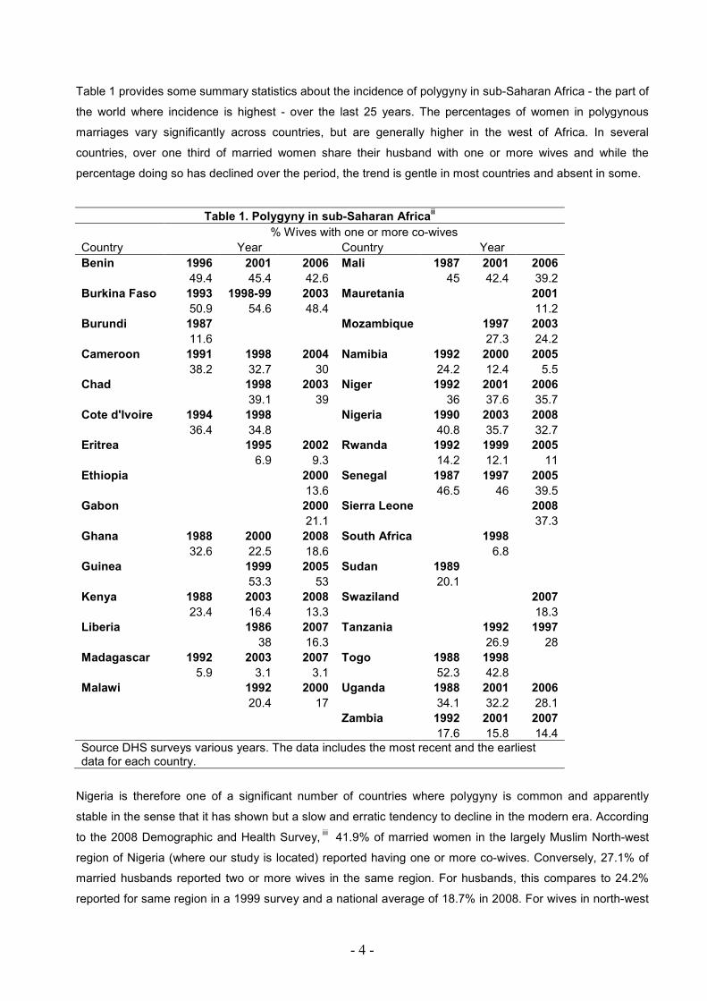


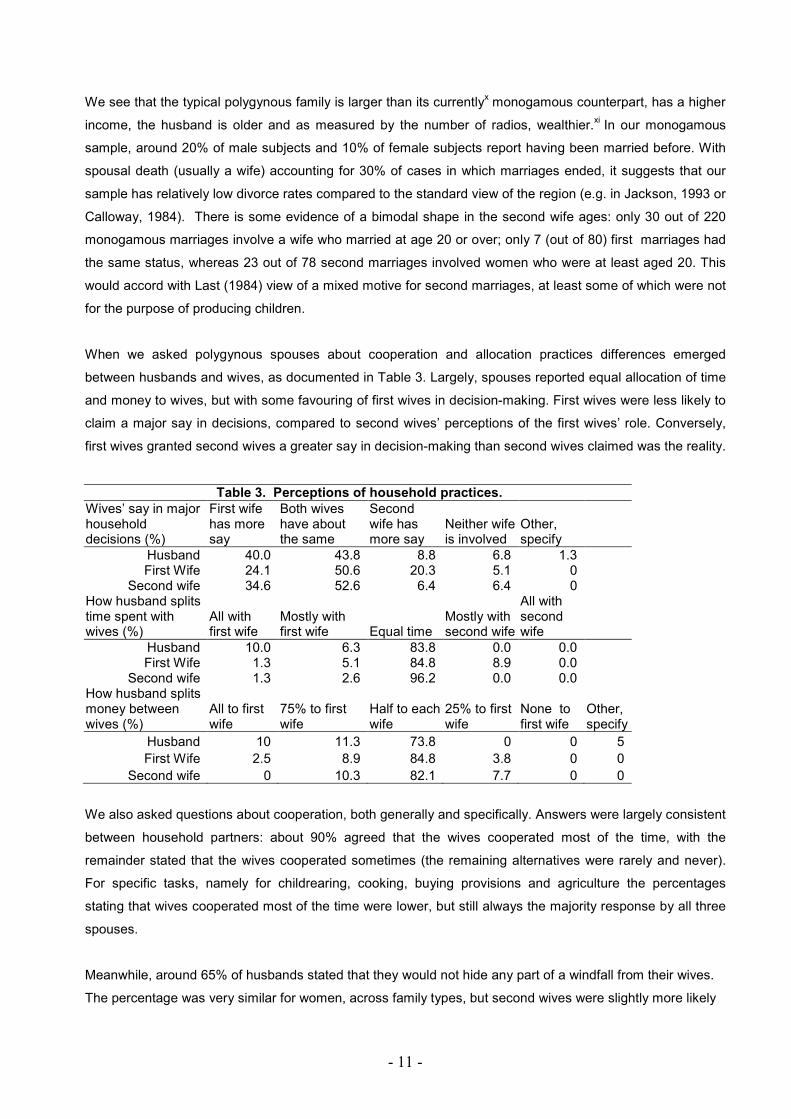
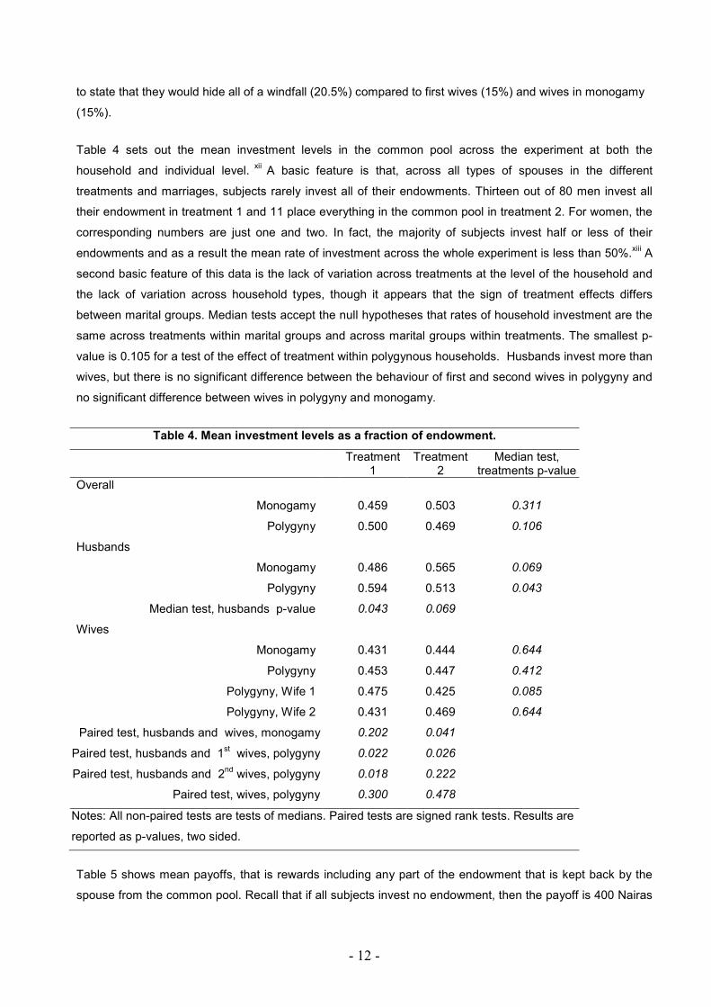

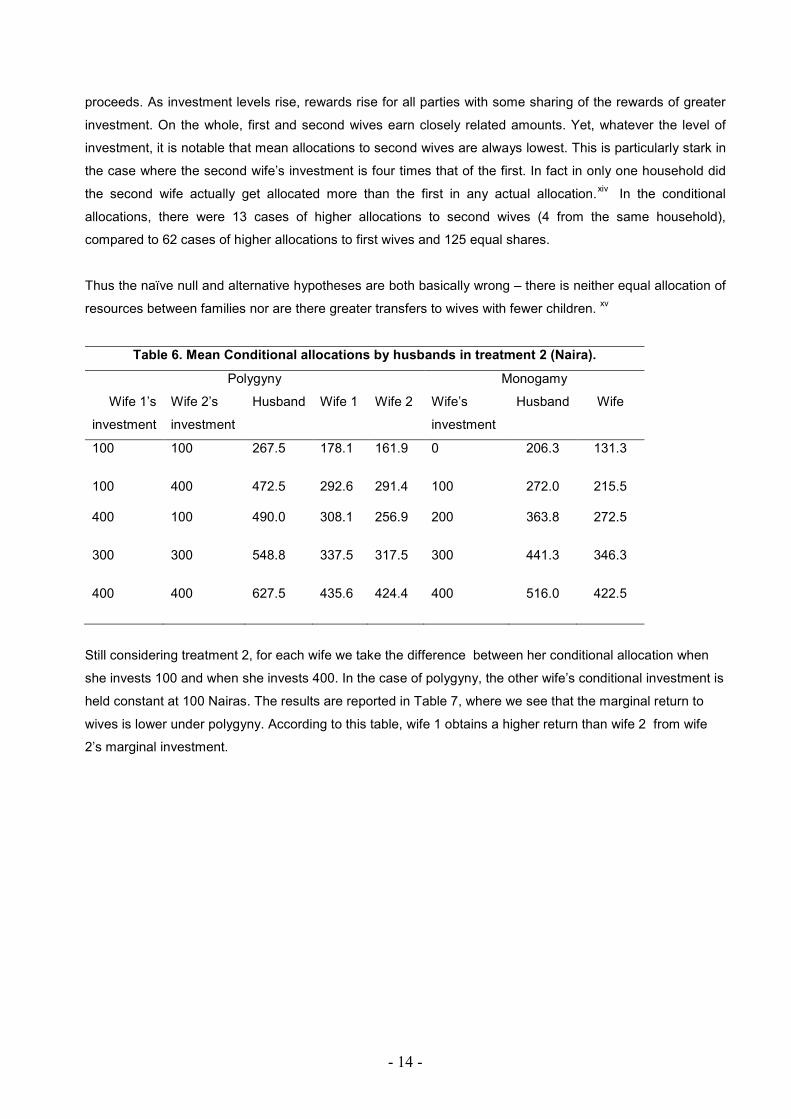
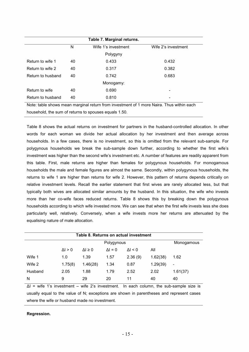
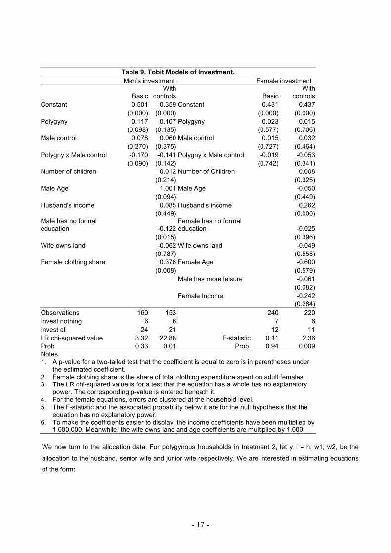
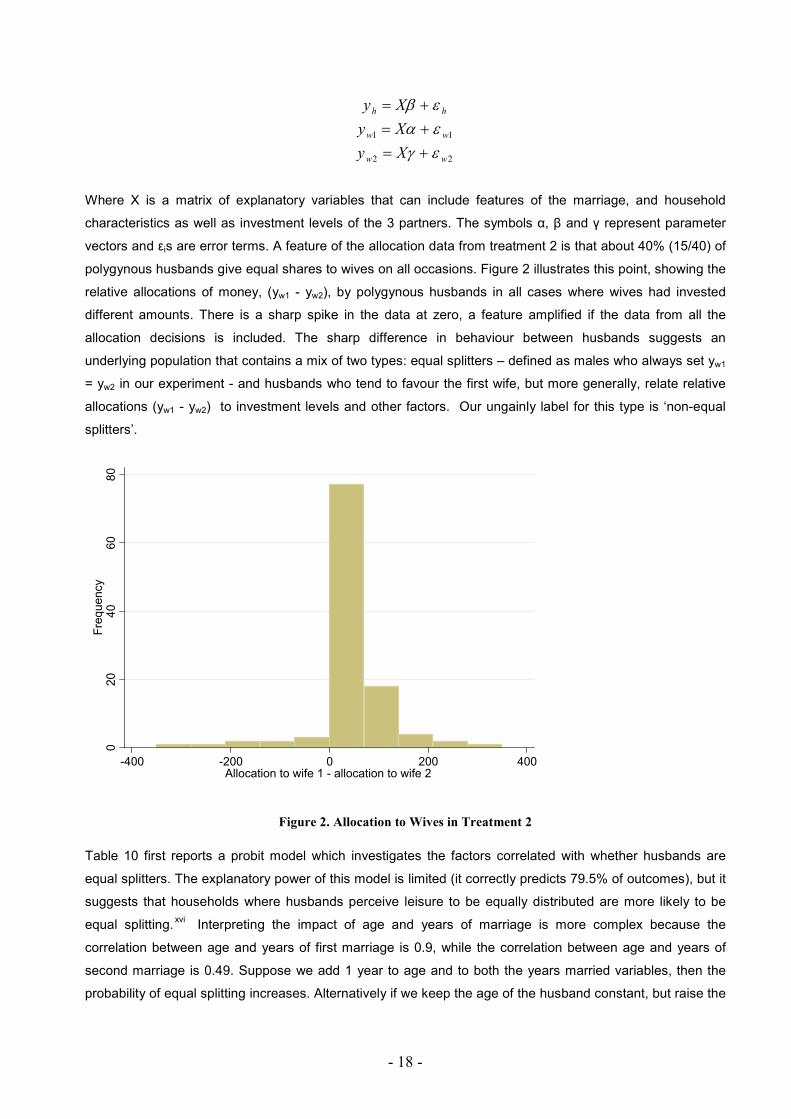
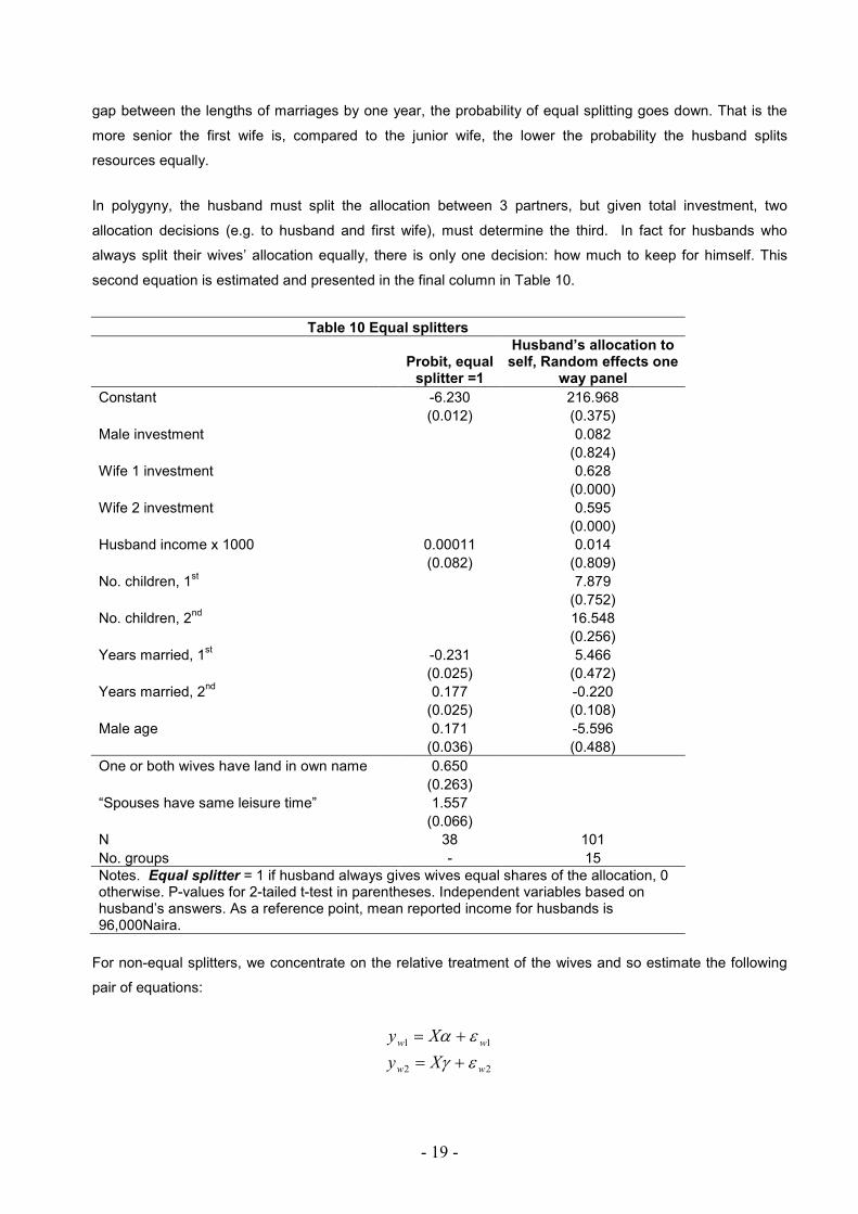
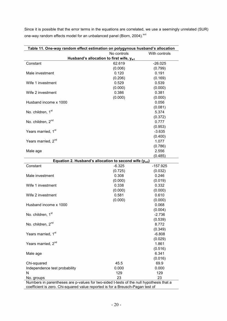


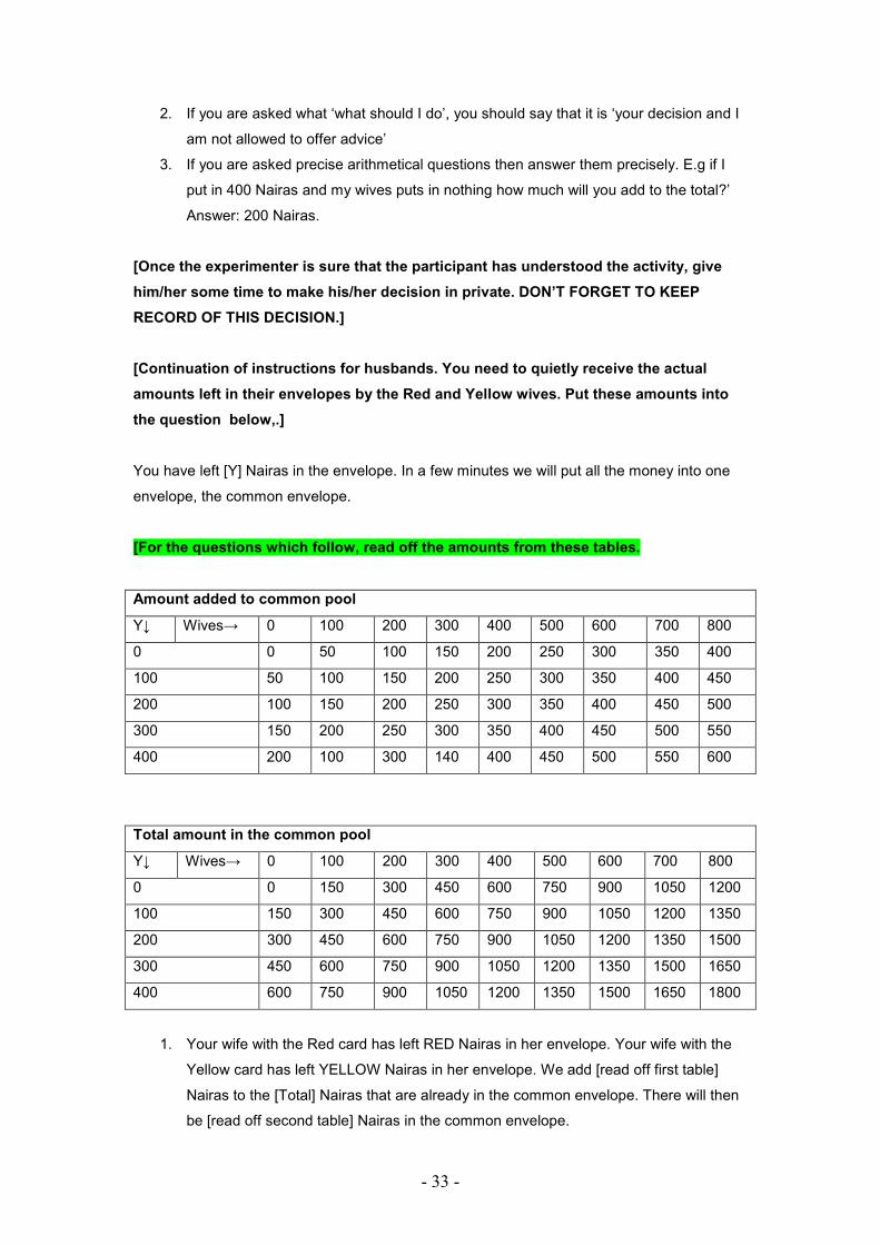


![Polygamy Nigeria exp02[1] - gov.uk...The Lion’s Share: an Experiment on Polygamy in Northern Nigeria. Alistair Munro**, Cecile Jackson*, Bereket Kebede*, Nitya Rao*, Marcela Tarazona*,](https://static.documents.pub/doc/80x56/5e908c84f1b031267a448cfa/polygamy-nigeria-exp021-govuk-the-lionas-share-an-experiment-on-polygamy.jpg)


