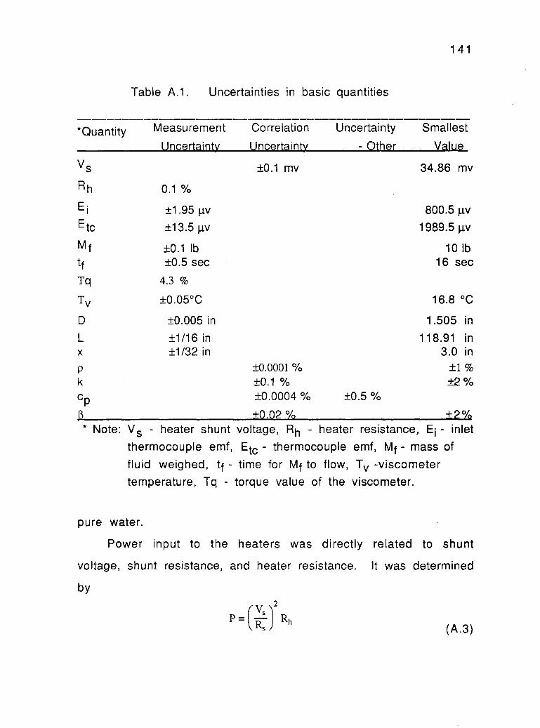
AN ABSTRACT OF THE THESIS OF YongJin Kim for the degree of Doctor of Philosophy in Mechanical Engineering presented on April 27. 1990 Title: An Experimental Study of Combined Forced and Free Convective Heat Transfer to Non-Newtonian Fluids in The Thermal Entry Region of a Horizontal Pipe Redacted for Privacy Abstract approved: James R. Welty \, The case of combined free and forced convection heat transfer in non-Newtonian fluids was experimentally investigated in uniformly-heated horizontal tubes with laminar flow in the thermal entry region. Velocity profiles were fully developed at the entrance to the heated sections of the tubes. Aqueous solutions of sodium carboxymethylcellulose(CMC) were used; their behavior showed a reasonably good fit into the power-law model, 't = K Yn. A range of polymer concentrations was chosen to attain several degrees of pseudoplastic behavior. The power-law constants, K and n, were determined using a rotational viscometer. The test sections used were made of copper with inside diameters of 3.823 cm and 5.042 cm and lengths of approximately 300 cm. Twenty two of 25 total runs displayed noticeable secondary
Transcript
AN ABSTRACT OF THE THESIS OF
YongJin Kim for the degree of Doctor of Philosophy in Mechanical
Engineering presented on April 27. 1990
Title: An Experimental Study of Combined Forced and Free
Convective Heat Transfer to Non-Newtonian Fluids in
The Thermal Entry Region of a Horizontal Pipe
Redacted for PrivacyAbstract approved:
James R. Welty \,
The case of combined free and forced convection heat transfer
in non-Newtonian fluids was experimentally investigated in
uniformly-heated horizontal tubes with laminar flow in the thermal
entry region. Velocity profiles were fully developed at the entrance
to the heated sections of the tubes. Aqueous solutions of sodium
carboxymethylcellulose(CMC) were used; their behavior showed a
reasonably good fit into the power-law model, 't = K Yn. A range of
polymer concentrations was chosen to attain several degrees of
pseudoplastic behavior. The power-law constants, K and n, were
determined using a rotational viscometer.
The test sections used were made of copper with inside
diameters of 3.823 cm and 5.042 cm and lengths of approximately
300 cm.
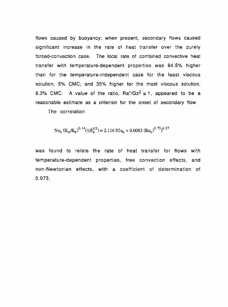
Twenty two of 25 total runs displayed noticeable secondary
flows caused by buoyancy; when present, secondary flows caused
significant increase in the rate of heat transfer over the purely
forced-convection case. The local rate of combined convective heat
transfer with temperature-dependent properties was 84.5% higher
than for the temperature-independent case for the least viscous
solution, 5% CMC; and 35% higher for the most viscous solution,
8.3% CMC. A value of the ratio, Ra*/Gz2 -a- 1, appeared to be a
reasonable estimate as a criterion for the onset of secondary flow.
where ab indicates the average bulk condition. They claimed this
equation to have ±40% accuracy.
Yousef and Tarasuk [169] examined the influence of free
convection with air in the entrance region of a horizontal tube.
Three regions in the entry region were considered; those were 1)
near the tube inlet where free convection is dominant, 2) further
downstream where forced convection becomes dominant, and 3) far
from the tube inlet where the mean Nusselt number becomes
constant. They found that free convection had a significant effect
12
on heat transfer near the entrance to the tube. Comparisons were
also made with several correlations used in combined convection in
an isothermal horizontal tube.
In the thermal entrance region for flow in horizonal tubes with
uniform wall heat flux, experimental work on laminar combined
convective heat transfer was carried out by McComas and Eckert
[95], Mori et al [109], Hussain and McComas [63], and Lichtarowicz
[83] for air; Shannon and Depew [141], Petukhov and Polyakov
[127,128], Kupper, Hauptmann, and lqbal [77], and Berg les and
Simonds [10] for water; and Shannon and Depew [140] for ethylene
glycol.
Using a boundary layer model, Siegwarth and co-workers [151]
studied the effect of secondary flow for the cases of Pr=1 and
P rw) in a heated horizontal tube. The temperature at the inside
surface did not vary circumferentially when a uniform heat flux
was specified at the outer wall of the tube. They obtained a
solution for the case Pr---)oo in the fully developed region as follows:
Nu = 0.471 Ra1/4 (2.2)
which agrees quite well with the experimental data of Siegwarth
and Hanratty [150] using a 2.5-inch I.D., 1-inch thick aluminum pipe.
Ra indicates p213ga3AT cp/kg where a means tube radius. It is noted
that the boundary condition used [151] is different from the uniform
circumferential heat flux condition applied to thin-wall tubes.
A theoretical analysis of combined forced and free convective
heat transfer in laminar boundary layer flows was done by Acrivos
13
[2]. The momentum equation, coupled with the energy equation
including the gravitational force term in two-dimensional flows
was solved. He used GrPr1/3/Re2 for large Prandtl numbers and
Gr/Re2 for Pr«1 as controlling parameters which indicate the
relative importance of forced and free convection.
The experimental investigation by Morcos and Berg les [108] on
combined convection in fully developed laminar flow throughout a
uniformly-heated horizontal pipe yielded the following correlations:
Nuf = {( GrP11."
(4.36)2f
+ 0.055(2.3)
for 3x10⁴ < Ra < 106, 4 < Pr < 175, and 2 < Pw < 66 where Pw is tube
wall parameter, hdi 2/Kwt. d1 and t indicate inside tube diameter
and tube thickness, respectively. f means the evaluation of
properties at fluid film temperature. Combined laminar convection
has also been investigated experimentally, in uniformly-heated
horizontal tubes, by Depew, Franklin and Ito [35].
Numerous analytical solutions on combined convective heat
transfer have been proposed for fully developed Newtonian flow by
Faris and Viskanta [41], Hwang and Cheng [64], Newell and Bergles
[112] and Hong, Morcos, and Bergles [62]. Cheng and Ou [19]
investigated combined laminar convection in the thermal entrance
region of horizontal tubes with uniform wall heat flux for large
Prandtl number fluids. From their theoretical results, asymptotic
Nusselt numbers for the fully-developed case were evaluated as
Nu. = 4.36 + 0.286 (Ra)1/4
14
(2.4)
Nu. = 3.4 + 0.303 (Ra*)1/4 for Ra*>10 (2.5)
where Ra = gf3a4q"/v2k and Ra* = gf3(Twavg-Tb)(2a)3/vk. a and v are
the radius of tube and the kinematic viscosity, respectively. Nu,. is
the asymptotic Nusselt number.
Analytical solutions have been examined by a number of
investigators for combined convective heat transfer in a horizontal
pipe with an isothermal boundary. Of note are papers by Ou and
Cheng [120], Hieber and Sreenivasan [60], and Hieber [59]. Hieber
and Sreenivasan obtained a solution using the large-Prandtl-number
assumption in the entrance region where the velocity and the
temperature fields are developing simultaneously.
Yao [167,168] obtained asymptotic solutions for the developing
entry length problem by perturbing the solution for developing flow.
Hishida, Nagano and Montesclaros [61] generated numerical
predictions for combined convection in the entrance region of an
isothermally heated horizontal pipe, which are reported to be
applicable to a fluid of arbitrary Prandtl number. Hieber [58]
attempted to establish a correlation which includes all
experimental heat transfer results for laminar mixed convection in
an isothermal horizontal tube. His correlation was found to be good
for (Gr Pr)1/4 44. Data beyond this range fit the laminar
correlation of Eubank and Proctor [40] quite well.
In recent years Coutier and Greif [29] have investigated
15
laminar flow and heat transfer within a horizontal isothermal tube
both experimentally and theoretically. Since free convection
effects coupled to axial motion create a three-dimensional flow
inside the horizontal tube, they analyzed the flow behavior and the
heat transfer using a three-dimensional numerical model. Their
numerical results for the temperature profiles in a developing flow
throughout the entire length of the short exchange tube agreed well
with the data from their experiments and with numerical data from
Ou and Cheng [120). Secondary flow was observed over the entire
range of conditions they considered.
2.2 Laminar convective heat transfer to non-Newtonian fluids
The non-linear relationship between the stress tensor and the
deformation strain tensor makes convective heat transfer to non-
Newtonian fluids difficult to model by numerical and analytical
methods. Many empirical models [152, p. 6-9) have been proposed in
the literature for non-Newtonian fluids. Most commonly used for
research on fluid dynamics and heat transfer of non-Newtonian
fluids is the power-law or Ostwald-de Waele model
Txy = -K (du/dy)n (2.6)
where K is the consistency index and n is the flow behavior index.
For Newtonian fluids K is the coefficient of viscosity and n is equal
to 1. The present study also employs the power-law model.
16
The simple classical problems of fluid dynamics and heat
transfer up to about 1960 have been well reviewed by Metzner [98]
and Metzner and Gluck [100]. Bassett [8] and Shenoy and Mashelkar
[147] have also reviewed in detail the publications on convective
heat transfer to non-Newtonian fluids. The following sections will
be limited to a review of laminar convective heat transfer to non-
Newtonian fluids in both external and internal flows.
2.2.1 External flows
The theoretical analysis of flow past an external surface with
power-law fluids under laminar forced convection has been
presented by Acrivos, Shah and Petersen [4]. They applied
similarity variables to the momentum equations, and estimated
local heat transfer rates using Lighthill's approximate formula. It
was assumed that the thermal boundary layer is much thinner than
the shear layer, i.e., their modified Prandtl number was very large.
Schowalter [136] showed that similar solutions exist for
external flows of pseudoplastic power-law fluids. For two-
dimensional flow the solutions were analogous to those obtained
for Newtonian fluids. For three-dimensional flow, however,
similarity solutions were much more restrictive than for Newtonian
fluids.
A numerical solution for forced convection flow of power-law
fluids under a right-angle wedge with an isothermal surface was
obtained by Lee and Ames [80] by solving the boundary-layer
17
equations. The transformation group method, which has been
described by Ames [6], was used for their numerical approach.
Transformations of the boundary-layer equations for cases of
a steady-state boundary layer, an unsteady-state bounday layer, the
thermal boundary layer, simultaneous free and forced convection,
and free convection in general for pseudoplastic and dilatant fluids
has been presented by Berkowski [11] without completing to analyze
rigorous solutions and the implications of various dimensionless
groups encountered for different problems.
Denn [34] extended boundary-layer solutions to include the
entire class of wedge (Falkner-Skan) flows for elastic fluids with
shear dependent viscous and normal stress relations. He obtained a
set of ordinary differential equations for the boundary layer flow of
a general elastic fluid away from the leading edge of the submerged
object. It was concluded from his several solutions that the effect
of fluid elasticity on drag depends on both the system geometry and
fluid parameters.
Tien et at [158] first investigated the thermal instability of a
horizontal layer of an inelastic power-law fluid heated from below.
Critical Rayleigh numbers were obtained as functions of the flow
behavior index; the critical Rayleigh number was shown to decrease
with the flow behavior index. It was assumed that instability
would occur at the minimum temperature gradient at which a
balance can be steadily maintained between the kinetic energy
dissipated by viscosity and the internal energy released by the
buoyancy.
Ozoe and Churchill [121], Parmentier et at [123], and
18
Parmentier [122] have also investigated the problem of free
convection in a horizontal layer of an inelastic non-Newtonian fluid
heated from below. Shenoy and Mashelkar [146] have suggested that
the Ellis fluid model (see chapter I.), as used by Ozoe and Churchill
[121], is superior to the model used by Tien et al.
A theoretical study of free convective heat transfer to power-
law fluids with steady, laminar boundary layer flow from
arbitrarily shaped two dimensional or axisymmetric bodies was
recently carried out by Chang, Jeng, and Dewitt [15]. The effect of
the convective term in the governing momentum equation was
included even though non-Newtonian fluids generally have high
Prandtl numbers. Universal functions, which are independent of
geometry, were obtained.
Parmentier [122] and Parmentier et al [123] emphasized that,
for pseudoplastic fluids ( 0.3 < n < 1 ), the structure of thermal
convection cells at steady state is the same as for Newtonian
fluids. They also found that for values of n below 0.3 the fluid
deformation tends to become more localized and significant regions
of stagnant fluid develop.
Pierre and Tien [129] and Tsuei and Tien [159] have obtained
experimental results for free convection of a non-Newtonian fluid
in a horizontal layer
19
Vertical flat plate
Laminar free convective heat transfer to power-law fluids
was examined by Acrivos [1] for the case of a vertical plate with
constant temperature. He developed an expression for the local
Nusselt number from the exact asymptotic solution of the
appropriate laminar boundary layer equations. His solution can be
applied to a two-dimensional surface or a surface of revolution
about an axis of symmetry when the power-law Prandtl number,
pcp )( K 2 /(n+1)L(n-1)/2(n+1) [gi3 (TwT.:,)]3(n-1)12(n+1)
is greater than 10.
An experimental investigation of free convective heat transfer
in a non-Newtonian fluid was made by Reilly et al [131]. Their
results were consistent with Acrivos' [1] analytical results.
Na and Hansen [111] have shown that similarity solutions for
laminar free convection of non-Newtonian fluids can be obtained by
using group theoretic methods. Studies on laminar free convection
to non-Newtonian fluids have been also conducted by Tien [155],
Dale [30], Dale and Emery [31 ], and Kleppe and Marner [71]. Tien
[155] obtained approximate solutions using an integral method and
the power-law model with high Prandtl number situations for cases
of an isothermal plate, a non-isothermal plate, and a plate with
uniform heat flux.
Dale and Emery [31] measured and predicted numerically the
20
local heat transfer, temperature, and velocity distributions
between a vertical constant flux plate and several concentrations
of pseudoplastic fluids. Flow indices varied from 0.395 to 1.0, and
the fluid consistencies were 30 to 2300 times those of water. The
heat transfer in their study was expressed as the following
generalized non-Newtonian correlation:
where
Nux= C (Gr* Pr*x)(3n+2) (2.7)
* gi3(1Tjx(n+2)/(2n)Grx =
K )2/(2n)CpJ (2.8)
* C (K )1/(2-n) 2(1-n)/(2-n)X -_ Pk X
(2.9)
By transforming the governing partial differential equations
into ordinary differential equations, Chen and Wollersheim [18]
solved the problem of laminar free convective heat transfer for the
case of a vertical plate with uniform heat flux. Solutions for
constant heat flux and variable wall temperature were also
obtained for laminar free convective heat transfer to a power-law
fluid from a vertical flat plate by Shenoy [142].
Shenoy and Mashelkar [147] have discussed the appropriate
boundary and compatibility conditions in detail. These conditions
21
were not satisfied for the velocity and temperature profiles used by
Tien's [155]. These conditions were later used by Shenoy and
Ulbrecht [145] who obtained an integral solution for laminar free
convective heat transfer from an isothermal vertical flat plate to a
power-law fluid.
A theoretical analysis for laminar mixed convective heat
transfer to inelastic non-Newtonian fluids in external flows has
been studied by Kubair and Pei [75] for the case of a vertical flat
plate with constant wall temperature. They concluded that:
1. the combined effects of free and forced convection for non-
Newtonian laminar boundary-layer flow are satisfactorily
characterized by the dimensionless group, P = Gr'/Re'2/(2-n),
where a modified Reynolds number
pu2-nxnRe'
and a modified Grashof number
jx(n+2)/(2-n)Gr' =
2/(2-n)
(2.10)
(2.11)
2. based on the asymptotic limits in pure flows, the effect of
free convection is negligible for P < 0.1 and the effect of
forced convection is apparent even at P = 5.0 for Newtonian
fluids. At higher Prandtl numbers the free convection effect
22
may be predominant at somewhat lower values of P both for
Newtonian and non-Newtonain fluids.
3. for opposing flows the phenomenon of zero shear is strongly
influenced by non-Newtonian behavior.
However, a number of errors were later found in their analysis.
Shenoy [143] pointed out that the controlling parameter, P, would be
constant only under limited conditions, which Sparrow et al [153]
have specified and explained in the case of Newtonian fluids under
combined convection flow. He also indicated that the continuity
equation is not satisfied by their dimensionless groups. Their
statement that their boundary equations reduce correctly to the
Newtonian forms and does not have this limitation was found to be
incorrect.
Churchill [24] has presented a correlation for laminar
assisting combined convection flow of Newtonian fluids, which is
also valid for non-Newtonian power-law fluids. The form of the
correlation is
Nu3 =Nu3x,F +Nu3x,N
x,M (2.12)
where Nux,M' Nux,F' and Nux,N are local Nusselt numbers based on
the local distance x on the heat-transferring surface for mixed,
forced, and free convection, respectively. Later Ruckensten [132]
has established his correlation [24] using an approximate
interpolation procedure. Using the form above, Shenoy [143] has
proposed an equation for predicting the combined convective heat
23
transfer rate to the flow of power-law fluids past an isothermal
vertical flat plate. For pure forced-convective heat transfer the
correlating equation is from Acrivos et al [4]. The relation of
Shenoy and Ulbrecht [145] was used for the free convective heat
transfer term. Greatest accuracy for non-Newtonian fluids would
be cases of large Prandtl numbers.
Although the power-law model, which is a two-parameter
model, is popular for solving many engineering problems, the
Sutterby and Ellis model (three-parameter model) turns out to be
more useful, particularly when the stresses or strain rates are
small. Laminar free convection from a vertical flat plate has been
analyzed by Shenoy and Mashelkar [146] who used these two time-
independent models.
Lin and Shih [84] analyzed laminar mixed convection vertically
static or moving plates and power-law fluids for both the
prescribed surface temperature and prescribed wall heat flux cases.
The local similarity method [85,86] has been employed to
demonstrate nonsimilarity due to buoyancy effects, non-Newtonian
behavior, and moving boundary conditions. They showed that the
method of local similarity is useful for the study of power-law
fluids.
Vertical cylinder
Recently, Wang and Kleinstreuer [162] numerically investi-
gated laminar mixed convection with power-law fluids adjacent to
24
vertical slender cylinders. Using a coordinate transformation and
an implicit finite-difference method, they solved the non-similar
problem to examine the effects of transverse curvature, power-law
index, buoyancy parameter, and generalized Prandtl number on the
local heat transfer and skin friction coefficients. Thermal boundary
conditions used were both constant temperature and uniform heat
flux.
Horizontal cylinder
An experimental investigation for free convective heat
transfer from a horizontal cylinder to moderately elastic drag-
reducing polyethylene oxide solutions has been carried out by Lyons
et al [88]. They observed a decrease in Nusselt numbers, compared
to Newtonian fluids, with increased polymer concentration without
any quantitive comparison.
Local free convective heat transfer from a horizontal
isothermal cylinder to non-Newtonian power-law fluids has been
investigated numerically and experimentally by Gentry and
Wollersheim [47]. The local Nusselt numbers obtained experi-
mentally showed good agreement with their [47] similarity and
integral solutions.
Using concentrated corn starch suspensions in aqueous sucrose
solutions, Kim and Wollersheim [70] obtained experimental data for
free convection from a horizontal cylinder to dilatant fluids with
both isothermal and uniform heat flux surface boundaries. Their
data for an isothermal horizontal cylinder were in excellent
25
agreement with the theoretical solutions presented by Gentry and
Wollersheim [47].
In the case of external flows of viscoelastic fluids Shenoy
[144] obtained an expression for combined laminar forced and free
convective heat transfer in the stagnation region of an isothermal
horizontal cylinder using an approximate procedure. The correlation
which was obtained using a similar manner to Ruckenstein [132] and
Shenoy [143] is of the form:
NU3avR,M = u3avR,F + Nti3avR,N (2.13)
He noted the effects of viscoelasticity as well as free convection
to increase the heat transfer. Based on the radius of the cylinder
indicate average Nusselt number forNU3avR,M' Nu3avR,F and NU3avR,N
mixed convection, forced convection, and free convection,
respectively.
Ng and Hartnett [114] recently reported an experimental study
for free convection to horizontal wires, whose diameters were of
the same order or smaller than the boundary layer thickness of free
convection. Test fluids were Carbopol 960 and Carbopol 934, which
are both pseudoplastic. In order to reduce the results for the three
temperatures tested to a single curve, a reduced shear rate, 7r = 7
exp(B/T), which is a form proposed by Christiansen et al [23], was
introduced. The constant B was determined experimentally. By
transforming Acrivos' [1] analytical results into a new set of
26
dimensionless Ng and Hartnett [113] showed that the Nusselt
number may be expressed as
Nu = C RaN 1/(3n+1) (2.14)
where RaN indicates the Rayleigh number for power-law fluids. A
final equation based on their experimental data is
Nu = (0.761 + 0.431 n) RaN
Sphere
1/{2(3n+1)} (2.15)
A solution of the two-dimensional boundary layer equations
obtained by Acrivos et al [4] has also been presented for forced
convective heat transfer from a sphere to power-law fluids at large
Reynolds numbers. By using a Mangler-type transformation [135],
Acrivos [1] has provided and extended the theory for free convective
heat transfer from a two-dimensional surface to the three-
dimensional axisymmetric case.
Amato and Tien [5] carried out an experimental investigation
on free convective heat transfer from isothermal spheres to
aqueous polymer solutions of CMC-7H and Polyox WSR-FRA. The
local heat transfer variation on a sphere as a function of the
angular distance from the stagnation point showed good agreement
with the values of Acrivos [1].
Yamanaka and Mitsuishi [166] examined combined forced and
27
free convective heat transfer from spheres to aqueous solutions of
some polymers. They correlated their experimental data with an
empirical equation obtained by extending the Newtonian correlation
for combined convective heat transfer using the power-law model.
They applied the method proposed by Acrivos and Goddard [3] to
derive this equation. Solutions of 2.61% MC (methylcellulose), 5.52%
CMC, 0.74% SPA (sodium polyacrylate), and 1.48% PEO (polyethylene
oxide) were used as test liquids. Their equation correlated the
experimental data at Peclet numbers below 1000 and small
Reynolds numbers with a maximum and a mean deviation of 67.7%
and 29.3%, respectively. Since polymer solutions generally have
high Prandtl numbers, Peclet numbers are large in most cases.
2.2.2 Internal flows
For external flows the boundary development layer is
continuous. However, for internal flows, such as flows through
heated or cooled tubes, the boundary layer development is
constrained. While very few studies involving free convective heat
transfer to non-Newtonian fluids in internal flows have been
conducted, many studies on forced-convective heat transfer to non-
Newtonian fluids have been carried out by numerous investigators.
Parallel plates
Temperature profiles for flow between two parallel plates,
with one stationary and the other moving at constant velocity, have
28
been obtained by Tien [156]. He has provided temperature profiles
for two cases: both plates maintained at constant temperatures, and
one plate maintained at constant temperature while the other is
insulated.
Tien [157] also extended the asymptotic solutions of the
classical Graetz-Nusselt problem to the case with a non-Newtonian
fluid flowing between parallel plates. Instead of an exact velocity
profile, the approximation developed by Schechter [133] was used.
Both studies [133,157] were carried out for the Power-law model.
Matsuhisa and Bird [94] summarized many solutions to flow
problems using the Ellis model. Problems considered were
isothermal flow between flat plates, in circular tubes, in a film
flowing along an inclined plate, in annuli (axial, tangential and
radial), and nonisothermal flow in circular tubes with both uniform
heat flux and constant temperature wall conditions.
A numerical approach was attempted by Vlachopoulos and John
Keung [161] to examine heat transfer to a power-law fluid flowing
between parallel plates with constant wall temperature. As the
flow index, n, increased, the bulk temperature and the local Nusselt
number were observed to decrease. These results agree with Tien's
[157] work. It was also concluded that viscous dissipation had a
significant effect on heat transfer in a parallel plate channel.
Horizontal pipe
Analytical studies by Lyche and Bird [87] and Schenk and Van
29
Laar [134] can be considered as extensions of the classical Graetz-
Nusselt problem. They used velocity profiles appropriate to the
power-law model and the Prandtl-Eyring model, respectively. A
separation of variables similar to that used by Sellars, Tribus, and
Klein [138] for a Newtonian fluid was employed in Lyche and Bird's
work for a power-law pseudoplastic fluid.
By using ammonium alginate, applesauce and banana puree
which are predominantly pseudoplastic in character, Charm and
Merrill [17] investigated the heat transfer behavior of these fluids
in streamlined flow.
Analytical studies employing the power-law model have also
been conducted by Whiteman and Drake [164], Wissler and Schechter
[165], Pawlek and Tien [125], Foraboschi and de Federico [42] and
Kumar [76].
The analogy between heat and momentum transfer was
extended by Metzner and Friend [99], to include non-Newtonian
fluids in turbulent flow through circular tubes. The analogy was an
extention of the theoretical relationship for Newtonian systems
suggested by Friend and Metzner [45].
Data for a polymer solution of water-carbopol were acquired
by Metzner and Gluck [100]. They accounted for buoyancy effects in
non-Newtonian flows in an isothermal circular pipe. The equation
Eubank and Procter [40] proposed was modified using the power-law
model in the following form:
0.4 1/30.141 /33n+1
Nup = 1.75 (- (K) [G, + 12.6( Grw Pr, IT)
30
(2.16)
where Ko and Kw are the consistency indices evaluated at the bulk
and wall conditions, respectively. All physical properties were
evaluated at wall temperatures and wall shear rates. Gee and Lyon
[46], Griskey and Wiehe [51], Forsythe and Murphy [44], and Collins
and Filisko [28] also took polymer melt data in circular tubes with
isothermal walls.
A temperature-dependent power-law model was used by Hanks
and Christiansen [54], Christiansen and Craig [22], Korayem [72], and
Forsyth and Murphy [44], and by Cochrane [25]. Christiansen and
Jensen [21] used a temperature-dependent Powell-Eyring model in
obtaining their solutions. Christiansen and Craig proposed the
following simple temperature dependent equation to represent the
pseudoplastic rheology:
ti = K [S exp(AH/RuT)]n (2.17)
where S is shear rate, Ru is the universal gas constant, AH is the
activation energy per mole for flow, and k, n, and A H/R u are
empirical constants which are presumably independent of
temperature. They solved the governing equations numerically for
heating of both Newtonian and non-Newtonian fluids, for steady,
laminar flow and heat conduction to a flow without free convection
and thermal energy generation in circular tubes with constant
31
surface temperature. They also took experimental data for two
pseudoplastic fluids, a 3% water suspension of CMC and a 0.75%
water solution of CPM (carboxypolymethylene), under conditions
where free convection was negligible. Comparisons between the
estimated Nusselt numbers and measured Nusselt numbers gave a
mean deviation of ±7%.
By adding the possibility of viscous dissipation to the power-
law model, Gill [48] obtained a series solution. The eigenvalues are
functions of a rheology parameter, n. For each new n, a new set of
eigenvalues must be calculated.
Instead of viscous dissipation, slurry flow with uniform heat
generation was considered in the region of Gzx <25n by Michiyoshi
and Matsumoto [102]. Using the Bingham plastic model, Michiyoshi
[101] and Michiyoshi et al [103] also investigated the heat transfer
for slurry flow in both the fully-developed and the thermal entry
regions with internal heat generation.
Using the power-law model and a numerical solution of the
continuity, momentum, and energy equations for two dimensional
flow, McKillop [96] obtained results on convective heat transfer for
pseudoplastic fluids. For the case of fully developed entry flow, a
7.5% increase in Nux for a change in n from 1 to 0.5 and a 119%
increase in Nux for a change in n from 1 to 0 were observed at Gzx =
100n.
An experimental study for heating and cooling of pseudo-
plastic fluids (water-CMC, water-carbopol, water-polyox and ethyl
alcohol-carbopol) under isothermal surface temperature heating and
32
cooling conditions was carried out by Oliver and Jensen [118]. They
showed that the free convection effect did not depend on the 'L/D
ratio, and the correlation equation suggested by Metzner and Gluck
[100] did not fit their data. They presented the following
relationship,
0.14
Nu!) = 1.75(K
-) [Gz + 0.0083 (GI., Prv,)0.75,1/3
,, (2.18)
They showed that the heat transfer rate was affected more by
buoyancy than by either non-Newtonian or temperature-dependent
viscosity effects. They claimed that less viscous non-Newtonian
fluids increase heat transfer by as much as 100%.
Inman [65] obtained power-law solutions for the fully-
developed region and circumferentially-varying heat flux, using a
rheological model that is not temperature-dependent.
Using the Ellis model, laminar heat transfer to non-Newtonian
fluids was studied for both isothermal uniform heat flux boundaries
by Mitsuishi and Miyatake [104]. They obtained eigenvalues for 5
values of the flow behavior index, n, for each solution.
Laminar heat transfer in a circular tube with uniform wall
heat flux was investigated by Mizushina et al [107] employing the
power-law with temperature-dependent consistency (K), and
applying a correction term (Kb/Kw)0.1/n" to Bird's [12] asymptotic
solutions. They also took data for glycerol, which is Newtonian, and
aqueous solutions of CMC in the range, 10< Gzx < 300, which
33
includes the end of the developing region and the beginning of fully-
developed conditions. Significant data scatter suggests that
possible buoyant effects were not considered.
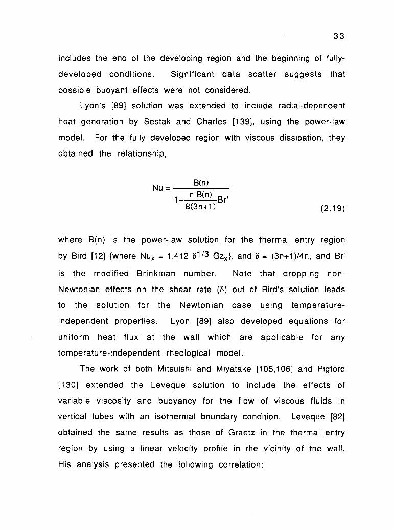
Lyon's [89] solution was extended to include radial-dependent
heat generation by Sestak and Charles [139], using the power-law
model. For the fully developed region with viscous dissipation, they
obtained the relationship,
BNu
B(n)
1 n B(n)Br'
8(3n+1) (2.19)
where B(n) is the power-law solution for the thermal entry region
by Bird [12] {where Nux = 1.412 81/3 Gzx}, and 8 = (3n+1)/4n, and Br'
is the modified Brinkman number. Note that dropping non-
Newtonian effects on the shear rate (8) out of Bird's solution leads
to the solution for the Newtonian case using temperature-
independent properties. Lyon [89] also developed equations for
uniform heat flux at the wall which are applicable for any
temperature-independent rheological model.
The work of both Mitsuishi and Miyatake [105,106] and Pigford
[130] extended the Leveque solution to include the effects of
variable viscosity and buoyancy for the flow of viscous fluids in
vertical tubes with an isothermal boundary condition. Leveque [82]
obtained the same results as those of Graetz in the thermal entry
region by using a linear velocity profile in the vicinity of the wall.
His analysis presented the following correlation:
Num = 1.75 81/3 Gz1/3
34
(2.20)
where 8 the shear rate ratio is equal to iew/8V/D with 7 W a function
of Gz,11b/11w, and Gr. The quantities 7 W and ri represent wall shear
rate and apparent viscosity, respectively. By evaluating 8x at the
axial mean wall temperature up to that point, they attempted to
compensate for the inaccuracy that resulted from specifying a
uniform shear all along the pipe wall. The difference between
Bird's result and their solution is only in the method used to
evaluate 8.
Han et al [53] reported the results of a study on axial pressure
distributions for the flow of molten polyethylene and polystyrene
through a circular tube (L/D = 4) at shear rates from 100 to 500
sec-1.
Cochrane [25,26] presented a numerical solution for the
coupled energy and momentum equations describing steady state
laminar flow of temperature-dependent power-law fluids. Pipe
flow and channel flow between two flat, parallel plates were
considered. A rheological model, ti = K eAH/RuT)n, was employed
to obtain results for both heating [25] and cooling [26]. When values
for dimensionless heat flux (4) = q"D/KT;), n, Pri, and AFI/RuTi were
taken as 2.0, 1, 1000, and 5, respectively, Nux increased by 5% at
Gzx = n/4 x 105 and by 14% at Gzx = 71/4 x 102 compared to the
temperature-independent solution.
Khabakhpasheva et at [69] and Kutateladze et at [78] showed
what was apparently the same set of data for the flow of a 1%
35
what was apparently the same set of data for the flow of a 1%
aqueous solution of polyacrilamide which is viscoelastic. No
elastic effects were found in circular tubes where conditions were
those of fully-developed, steady, laminar flow without free
convection.
Using temperature-dependent power-law fluids, the boundary
layer equations for flow in the entrance region with a uniform
velocity specified at the entrance were solved by Bader et al [7].
Their results were compared with data taken for aqueous
hydroxyethylcellulose and sucrose aqueous HEC alone. Entrance
Prandtl numbers ranged from 144 to 270, and the two fluids with n
= 0.85 and n = 0.62 were used. Their results, however, were hard to
interpret.
For fully-developed turbulent flow of power-law fluids at
large Prandtl numbers, a new correlation on heat transfer rates was
made by Krantz and Wasan [74].
By using a non-linear plastic (t = To + no in), Shul'man et al
[148] analyzed convective heat transfer in a circular pipe, to
include dissipation. The boundary layer equations with a uniform
wall heat flux were solved by Etchart and Welty [39], using a
temperature-dependent Powell-Eyring model. Rheological data for
several non-Newtonian fluids taken from the literature were used
in their analysis. They found that temperature effects on viscosity
had a major influence on heat transfer for the fluids analyzed. Heat
transfer was also affected, but to a lesser degree by non-Newtonian
flow behavior. They stated that the effect of viscous heat
36
dissipation on heat transfer would be significant for highly viscous
fluids with viscosities exhibiting moderate to heavy temperature
sensitivity. They also observed that the pressure drop is
significantly reduced when a fluid exhibits a temperature-
dependent viscosity.
Payvar [126] obtained fully developed temperature distri-
butions and asymptotic Nusselt numbers for three popular models -
the power-law, the Bringham plastic, and the Ellis model for a
uniform wall heat flux, considering the effect of viscous
dissipation using a procedure similar to that which he used for
parallel flat plates.
By employing a temperature-dependent non-linear plastic
model, the momentum and energy equations in the absence of radial
velocity terms were solved numerically by Forrest and Wilkinson
[43]. They obtained results for both heating and cooling. Viscous
dissipation effects were shown in their additional results.
For the thermal entry region flow, Bassett and Welty [9]
initiated an experimental study to determine the heat transfer rate
to laminar, forced flow of pseudoplastic fluids in a uniformly
heated circular pipe with fully developed velocity profiles at the
entrance, where Graetz number values varied between 240 and
38,000. They found that the local heat transfer rate was influenced
by temperature-dependent viscous properties much more than non-
Newtonian effects. They also observed that the intensity of
secondary flow patterns decreased with more viscous fluids and
increasing flow rate, and increased as the flow moved downstream.
Effects of viscous heating were not detected in the flow of fluids
37
tested with Brinkman numbers greater than 4.22 x 10³.
Experimental data, exclusive of two out of 26 runs, where free
convection was explicit in the results, were correlated as
Nux = 1.85 Gzx1/3-0.0318x (2.21)
which determines the heat transfer rate within 10% with a mean
error of 3.57% for flows without significant free convection
effects. Their experimental investigations led to conclusions that
the local wall shear rate controls the heat transfer rate and that
the shear rate is more profoundly influenced by temperature-
dependent viscous properties than by non-Newtonian behavior. They
also accounted for secondary flow due to buoyancy which can affect
the rate of heat transfer substantially far upstream of the usual
onset of full thermal development.
Laminar convective heat transfer of power-law pseudoplastic
fluids (methyl ether of cellulose, carboxypoly-methylene) in
circular conduits was investigated by Mahalingam et al [90), using
boundary conditions of uniform heat flux with a step change in heat
flux. Variations in the shear stress with shear rate for
temperatures between 80 F and 150 F were plotted for each
concentration to evaluate n and K. The exponent, n, was found to be
practically independent of temperature except for two
concentrations of methocel. Even these n values did not vary
greatly with temperature. So it was claimed that n may be assumed
a constant with temperature in any theoretical analysis. The
38
factor, K, was observed to decrease with increasing temperature
for each concentration. One of Bassett's conclusions [8] noted that
temperature-dependent fluid rheology is generally more important
in regard to the rate of heat transfer than the degree of
pseudoplasticity. The coefficient, K, was correlated as K = a ebt
where a and b are constants. Their [90] final correlation accounting
for pseudoplasticity, radial viscosity variation with temperature,
and free convection is of the form:
Kw
Nub 1)-1/3
= 1.46 [Gzb + 0.0083 (Grwprw)0.75]1/3(rb- 1-
(2.22)
where the absence of L/D in the free convection term is noted.
From a comparison of the numerical results with experimental data,
they concluded that analytical methods already available for the
Newtonian case may be extended to the non-Newtonian case.
Lakshminarayanan et al [79] studied heat transfer for heating
and cooling of pseudoplastic fluids in turbulent flow through
circular tubes. Experimental heat transfer data were correlated for
the heating and cooling of various aqueous polymer solutions
obeying the power-law model, allowing for the effect of
generalized Reynolds number and Prandtl number. They proposed the
following correlations for n' = 0.86-0.98, NRe,gen = 5000-22500, and
= 9-32:NPr,gen
N = 0.0710(N )-0.67 for heating (2.23)St Re, gen) Pr, gen
39
-0.33(N )4).67 for cooling (2.24)Nst = 0.0440(NRe, gen')
Pr, gen'
where
NRe, g en =DTIV2n p
8,1_1K( 3n+14n
Cp
KC 34n)11( 8V )11-1
Pr' k 4n J D J
(2.25)
(2.26)
n' indicates the slope of log versus s log (8V/D) plot.
Bird, Armstrong and Hassager [13] expressed laminar heat
transfer results in the thermally developing region by the following
asymptotic relationships:
for uniform heat flux
3n+1Nux 1.41 (4n
1
Gz3=(2.27)
where Gz > 25n, and for constant temperature
1
33n+1 )Nux = 1.16 (-4n
(2.28)
where Gz > 33n. The factor, [(3n+1)/4n]1/3, accounts for non-
Newtonian effect.
Gottifredi et al [49] developed a simple new analytical
approach to estimate local and mean heat fluxes for a constant wall
40
temperature to a fluid flowing in the laminar regime. They claimed
that their procedure could be applied to the analysis of both plane
and cylindrical geometries with the axial velocity distribution
given as an analytical function of position without any limitation on
the range of Graetz numbers. A marching technique was used and
comparisons were made with previous numerical estimates. The
agreement was very good.
Joshi and Bergles [67] investigated heat transfer with laminar
flow of two water-methocel pseudoplastic solutions in a circular
tube. Their following correlated equation was in generally good
agreement with the experimental data of Bassett and Welty [9]:
Nu vp,n
( Nuvp y Nucpm
Nu cp,n )\ Nucp,n=1
-0303 1
4.36 1 + (0.381 X+ )818
(2.29)
where, vp, and, cp, mean variable property and constant property,
respectively.
Cho and Hartnett [20] have described heat transfer and fluid
mechanics for non-Newtonian fluids in circular pipe flow. Laminar
heat transfer in the thermal entrance region of a circular pipe was
also reviewed by tabulating empirical correlations for uniform heat
flux and isothermal boundaries. Friction and heat transfer for
viscoelastic fluids were studied experimentally in turbulent pipe
flow of viscoelastic aqueous solutions of polyacrilamide by
Hartnett and Kwack [55], employing variables such as polymer
41
concentration, polymer and solvent chemistry, pipe diameter, and
flow rate. They also included a study of degradation effects. They
concluded that the friction factor and the dimensionless heat
transfer rate of the flowing fluid are determined only by the
Reynolds number, the Weissenberg number, and the dimensionless
distance. They suggested that their approach should be applicable
to other polymer solutions.
Vertical cylinders
Heat transfer studies on the vertical turbulent flow of water-
clay, water-powdered aluminum, ethylene glycol-graphite, and
ethylene glycol-aluminum slurries were carried out by Orr andDallavalle[119] for an isothermal wall. Their final correlation was
expressed as
)0.80( )0.33( )0.14
(11n3 0.027k Ps ) ks (2.30)
where s means suspension or slurry.
De Young and Scheele [33] and Marner and Rehfuss [93] studied
free convection in vertical pipes with constant heat flux conditions
for both upward and downward flow. Numerical solutions were
obtained for a power-law fluid. De Young and Scheele showed,
graphically, that the ratio Gr/Re at the maximum velocity varies
with the pseudoplasticity index n for both heated upflow and heated
downflow. It was seen from their figures that pseudoplastic fluids
42
set up flow instabilities earlier due to buoyancy effects. For
heated downward flow, opposite effects for the case of heated
upflow could not be predicted for a fluid with a power-law index
(less shear thinning) greater than n = 0.5 at a given value of Gr/Re.
It appeared that the critical Gr/Re increased with n and that, for
both upflow and downflow, the limiting Gr/Re was higher for
dilatant fluids than for pseudoplastic fluids. Unlike the case of
heated upflow, a decrease in the Nusselt number was found as
pseudoplasticity increased.
Marner and Rehfuss [93] showed three fully-developed velocity
profiles for n = 0.5. The velocity profile became more distorted
with an increasing Gr/Re. Nusselt numbers, flow stability, and
pressure drop were significantly affected by these velocity
distribution changes. As the pseudoplasticity index, n, decreased
the Nusselt number increased very significantly for a given value of
Gr/Re. While non-Newtonian effects tended to reduce the Nusselt
number in contrast to buoyancy effects for dilatant fluids, with
pseudoplastic fluids the buoyancy effects and non-Newtonian
behavior tend to increase the Nusselt number. They also observed
that the pressure drop increased with buoyancy, and that this effect
was much more significant for dilatant fluids than for
pseudoplastic fluids.
Combined convective heat transfer in a vertical tube with
upward flow for isothermal walls was investigated both
theoretically and experimentally by Marner and McMillan [92]. They
observed a point of maximum velocity profile distortion to exist
43
where an increase in dimensionless axial distance increased the
local Nusselt number. They also found that the pressure drop
increased with Gr/Re for all values of n. They obtained
experimental heat transfer data for carbopol solutions, which were
in agreement with theoretical predictions within ±15%.
Using a finite difference method to solve the coupled
continuity, momentum, and energy equations, Marner and Hovland
[91] investigated the simultaneous effects of viscous dissipation
and combined free and forced convection of power-law fluids for
fully-developed laminar flow in a vertical tube with uniform wall
heat flux. All properties were assumed to be constant except for
density which was considered a function of temperature. Velocity
profiles and Nusselt numbers were obtained as functions of the
flow behavior index(n), Gr/Re, and the product of E and Pr where E is
the Eckert number. Their results showed that the velocity profile
was distorted due to viscous dissipation. The Nusselt number
decreased while the friction factor increased with increased
viscous dissipation. Their numerical solutions are quite restrictive
because the power-law consistency index was assumed to be a
constant.
Rectangular duct
Fully-established friction factors for both purely viscous and
viscoelastic fluids in laminar and turbulent flow were measured in
a square duct by Hartnett et at [56]. Laminar friction factors for
44
both non-Newtonian fluids were in good agreement with the
equation for laminar circular pipe flow, 16/Re*. Turbulent friction
factors for purely viscous power-law fluids flowing through
rectangular ducts were in good agreement with the Dodge and
Metzner equation [37] for circular pipe flow of power-law fluids
with Re' replaced by Re*. Asymptotic friction factors for
viscoelastic fluids in turbulent flow through rectangular ducts
correlated well with circular tube expressions when compared at a
fixed Reynolds number, pVDh/rla, based on the apparent viscosity
evaluated at wall , and Dh is the hydraulic diameter. It was also
observed that the asymptotic fully-developed turbulent friction
factors in a square duct are much higher than the results of the
corresponding circular pipe at the some values of Re* (the Kozicki
Reynolds number).
Laminar heat transfer to a viscoelastic fluid flowing through a
rectangular channel was recently investigated by Hartnett and
Kostic [57]. In general, viscoelastic fluids behave as purely viscous
non-Newtonian fluids in fully-developed laminar pipe-flow because
the elastic properties of the fluid are not significant. High heat
transfer rates were measured compared with values for a purely
viscous fluid or a Newtonian fluid. Mena and co-workers [97] also
found higher heat transfer coefficients for viscoelastic fluids in
laminar flow through rectangular ducts than those for Newtonian
fluid. The elastic effects of a viscoelastic fluid, that make the
normal forces act differently on the boundaries, cause secondary
flows which produce a significant increase in heat transfer. The
friction factor, however, was unaffected by the presence of
45
elasticity in both studies [57,97]. They used an aqueous
polyacrylamide solution in a 0.5-aspect-ratio-rectangular-duct.
Rayleigh numbers ranged from 5,000 to 50,000 in their heat
transfer measurements. By comparing Nusselt numbers for the
viscoelastic fluid runs with the values for the water runs, they
concluded that a secondary flow, which was produced along both
upper and lower walls under the thermal boundary conditions given,
increased the heat transfer. They also found the effect of
elasticity on the pressure drop of a viscoelastic fluid to be
relatively small. Their measured dimensionless pressure drop
agreed well with the fully established friction factor, f = 16/Re*,
where
Re* = pVDh/[8 (a+/2-n)K](2.31)
and the constants a and b are 0.7276 and 0.2440, respectively. For a
circular duct a = 0.75 and b = 0.25 reduces the Re* to the
generalized Reynolds number introduced by Metzner [1965].
Tachibana and co-workers [154] reported a numerical analysis
of steady laminar flow of an inelastic power-law fluid (n < 1) in the
inlet region of rectangular ducts using finite-difference methods.
They also investigated experimentally the axial pressure
distributions from the entry region up to the fully-developed region
in rectangular ducts. Their results are as follows:
(a) In the inlet region with a power-law fluid the pressure
46
drop and the velocity in the duct center are smaller than with
a Newtonian fluid. Both pressure drop and velocity increase
with an increase in the the increasing power-law index. As in
the case of a Newtonain fluid, however, both the velocity in
the duct center and the pressure drop of a power-law fluid
decrease with an increase in the aspect ratio of the duct.
(b) The velocity profile in a power-law fluid is flatter than in
a Newtonian fluid.
(c) The entry region, with a power-law fluid, is longer than
that for a Newtonian fluid and decreases with an increasing
power-law index.
Others
An experimental study of the secondary and main flows was
carried out for viscoelastic polymer solutions, in an abrupt 2-to-1
circular expansion, by Halmos and Boger [52]. They measured the
developing centerline velocity and reattachment lengths for flow
through the abrupt circular expansion and observed that the
predevelopment of the flow field for viscoelastic fluids, which
decreases the size of the secondary cell, is directly related to
elasticity. It was also shown that the reattachment lengths of the
secondary cell are 13% and 29% less than those for inelastic fluids
at the same conditions. The size of the secondary cell is always
equal to or smaller than the inelastic prediction. They did not find
any significant deviation from inelastic behavior for We < 0.047.
47
We =VO
(2.32)
where 0, the Maxwell relaxation time, is expressed as
Pll -P22
2ti2Y (2.33)
V and D indicate the average velocity in the upstream tube and the
upstream tube diameter, respectively. P1
P22 means the normal
stress difference. For We > 0.12 the onset of flow instabilities
were detected in their measurements.
Non-Newtonian heat transfer in non-circular tubes has been
studied by Oliver [116] and Oliver and Karim [117]. Oliver and Karim
showed experimentally that flattened tubes produced higher
laminar-flow heat transfer coefficients than tubes of circular
cross-section. They stated that this increase is due to an increase
in the tube-wall shear rate and secondary flow patterns which
develop in viscoelastic liquids. The effect of secondary flows was
largest for a 1.5-aspect ratio. The aspect ratio was defined as the
ratio of the length of major axis of the flattened tube cross-section
to that of the minor axis.
48
Chapter 3. EXPERIMENTAL DESIGN AND SET UP
3.1 Experimental design
Appreciable free convection is known to occur with internal
laminar flows where Graetz numbers are greater than 10. To
achieve this value one needs either very low flow rates or very long
heated sections. The length of the test sections that could be
accommodated in the available facility was 10 ft. The entrance
sections were selected to be approximately 5 ft for flow
development. These entry lengths were found sufficient to ensure
fully-developed flow for all flow conditions used.
The flow remained straight from the entrance section inlet
through the exit of the test section. As discussed earlier, the test
fluids were dilute aqueous solutions of Carbose D-65. Their
behavior is pseudoplastic, and the degree of non-Newtonian flow
behavior increases with increasing concentration of solute.
Aqueous CMC displays flow behavior indices, n, as low as 0.6, and
maintains consistent behavior over a wide range of shear rates.
These fluids are non-toxic and their characteristics are well known.
They are also relatively inexpensive. They have been used
extensively by other non-Newtonian investigators.
Test section diameters of 1.5 and 2.0 inches were used in this
work. In general, smaller-diameter test sections have a large-
wall-thickness to diameter ratio, increasing the possibility of
significant heat conduction in the wall. Since the buoyancy
49
parameter Gr* varies directly with D4, smaller diameters also
reduce buoyancy effects.
The maximum possible Reynolds number was estimated for
each test section using the following Newtonian model, which is
conservative:
Le = 0.0575 D Re (3.1)
where Le is an entry length for fully-developed flow and D is inside
diameter of the test tube. The maximum Reynolds numbers for
fully-developed flow were 708 and 529 for the small and large test
sections, respectively.
The pressure drop along the entry and test sections was
estimated for this flow rate using the relationship [152, P 110],
AP=2K(324--II VnLri Rn+1
(3.2)
Values for AP were always found to be within the maximum
allowable pressure drop considering flange design, plastic wall
strength, pumping losses, and the possibility of viscous dissipation.
To avoid two-phase flow, the maximum design wall
temperature was chosen to be 185°F (85°C). Inlet temperatures
were adjusted to room temperature to minimize the possibility of
heat transfer to or from the fluid in the flow development section.
To reach this wall temperature for a range of flow rates, the
maximum power input required was estimated based on the Graetz
50
solution. This power input was scaled up by 50% to account for an
increase in heat transfer due to property variation with
temperature. The largest design value of input power was 6576
watts for the largest flow rate.
Therm couple Junction
Small Test Tube
Heating Strip
Large Test Tube
Figure 3.1. Cross section of test tubes
Axial locations selected for thermocouple placement were 3,
9, 18, 30, 48, 68, 91, and 117 inches from test section entrance.
These positions were chosen, based on the Graetz solution, to
capture important temperature information. The temperatures at
the bottom, side, and top of the tube wall at each axial position
were measured to examine the possible presence of buoyancy
effects. Figure 3.1 shows both test sections schematically.
Thermocouples could not be placed precisely at the positions 90°
and 180° in the small test section and 90° in the large test section
51
due to the equally-spaced heating strips. They were placed as close
as possible to these positions which were positioned at 0°,
98.2°,and 163.6° from the bottom in the small test section and at
0°, 102.9°, and 180° from the bottom in the large test section.
Keeping these design criteria in mind, flow rates for each fluid
and each test section were calculated for the desired range in
performance parameters. Six concentrations of CMC were employed
to cover the range in flow behavior, 0.6 < n < 1.0. In each run, the
power applied was that necessary to achieve a maximum wall
temperature of 185°F (85°C). Local heat tranfer rates were
collected for 127 < Gzx < 27474 and 5832 < Rax < 238011.
52
3.2 Experimental setup
3.2.1 Flow loop system
Figure 3.2 shows a schematic diagram of the entire test
apparatus. The pump drew fluid from the feed tank through a short
span of 2-inch piping. The fluid then flowed through 1.5-inch piping
to the tube side of the heat exchanger. Tap water was used on the
shell side for cooling. The test fluid continued to flow through 1.5-
inch piping to a static mixer which was used to eliminate any
temperature gradients. The fluid then passed through a 10-inch-
long viewing section. The bulk temperature was measured just
after the viewing section. The flow then entered one of the two
test sections. These were uniformly heated by electrical
resistance heaters attached to the walls. Wall temperature
measurements were taken at various axial positions along the test
section. The temperature measuring system consisted of
thermocouples, a reference junction, and a Leeds and Northrup K-4
potentiometer. A data acquisition system was used to record the
other miscellaneous temperatures. The data acquisition system
was not employed for wall temperature readings due to its
unacceptable accuracy.
Another static mixer was located at the exit to the test
section just before measuring the bulk temperature. The flow was
then directed to a weigh tank where the flow rate was determined.
The fluid entering the pump was mixed in the tank to keep it in a
Enclosure Boundary
Entrance Sections
--XView
Window
StaticMixer
Thermocouples
110 0 0 0 0 0Test Sections
Heat Exchanger
(EI
To Drain City Water-ix
By -Pass
Pump
Weigh Tank
Tank Mixer
001:40.1*
11
F77774:771.777:---1)
Figure 3.2. Schematic diagram of test loop
IIII
mominminominiomort
4a
Feed
Tank
Scale
54
uniform state.
The enclosure surrounding the apparatus extended from a point
1 ft upstream of the inlet flanges to the end of the static mixer
beyond the outlet of the test section. It was 24 inches wide, and 18
inches deep, and was filled with loose, vermiculite insulation.
3.2.2 Apparatus
Details of the apparatus are presented in this section.
Tank mixer
A 240 V DC motor, rated at 1/3 HP at 1750 rpm drove the tank
mixer through a 5 to 1 gear reduction unit. A 110 volt variable
transformer coupled to a 2:1 step-up transformer and a full wave
bridge rectifier supplied power. A 4-inch diameter, 3 blade, paddle
stirrer, which was scaled up from a design recommended by Union
Carbide Corp, was used for the mixing of water-soluble polymers.
Pump
A Moyno, 2L4, "progressing cavity" type was used. It had a tool
steel rotor and a Buna N rubber stator. The rotor was 18 inch long
and 1.5 inch in diameter. The fluid was pushed along in a cavity as
the rotor turned within the stator like a screw conveyer. The
manufacturer rated this pump at 24 gpm at 1200 rpm for fluids
whose viscosity ranged from 1 cp to 1000 cp. The output was
reported to be reduced to 9 gpm at 450 rpm for a 2500-5000 cp
55
fluid. As the exit pressure was increased to 80 psig, it was also
noted that these outputs dropped to from 24 to 22 gpm and from 9
to 6.7 gpm, respectively. Although the capacity was reduced by
increasing pressure and/or increasing viscosity, it provided a
steady, almost positive displacement flow. It also provided a flow
with less shearing action than a centrifugal pump or a gear pump.
A 240 volt DC motor rated at 2 HP and 1750 rpm drove the
pump. A V-belt and sheaves were used to reduce speed. Bassett [8]
noted that a 3.061 speed reduction resulted from the sheaves whose
diameters were 2.65 and 8.0 inches. Power was supplied to the
motor armature by a 220-volt variable transformer. Smoothing was
provided by 2000 gf of capacitance. Power was supplied to the
field with a line voltage of 208 V and a full-wave bridge rectifier.
Rectifier output was smoothed with 20 gf of capacitance.
Heat exchanger
The shell-and-tube heat exchanger with 2 tube passes had
about 20 ft2 of heat exchange area. The tubes were 5 ft long and
3/4 inch in diameter. City water was used in the shell side.
Static mixers
Construction of the static mixers was based upon a design
patented by Kenics Company. It consisted of a series of "bow tie"
elements. These elements were fabricated from 0.10 inch, annealed
aluminum sheet. They were formed from rectangular pieces 1.939
inches wide and 3.25-inches long by holding one end while the other
56
end was twisted 180 degrees. The number of clockwise elements
was equal to that of counter-clockwise elements. The ends were
notched and joined at right angles with epoxy glue. Element twist
directions were alternated in the joining process. This mixer was
designed to split, develop, and turn the flow with each new element.
A total of N elements would divide the flow into 2 N strata, the size
of each being D/2 N. Ten elements coated with epoxy paint were
inserted into a 2-inch, "hi-temp" PVC pipe 30 inches long.
Entrance sections
A slip-on type of standard 150 psi PVC flange was cemented on
each entrance section for attachment to the test sections.
Test sections
Stainless steel sleeves were silver-soldered to the both ends
of each test section and threaded. In addition to providing positive
mounting, the use of stainless steel helped to minimize heat loss.
A transition bushing was constructed from CPVC to provide the
minimum disturbance of flow between two different inside
diameters of both sections. PVC flanges connected the test
sections to other portions of the system.
a. Small section
A 10-ft, 13/32-inch-long piece of 1.505-inch ID, hard drawn,
copper tubing was used as the basic structure for this test section.
Its outside diameter was 1.625 inch; the wall thickness was 0.060
inch.
57
b. Large section
A 1.985-inch ID, 0.070-inch wall copper tube, having a length
of 10 ft, 7/32 inch, was used; the outside diameter was 2.125 inch.
A diagram of the test section assembly is shown in figure 3.3.
Power supply for heater
A Sorensen model DCR 300-35A, regulated DC supply, was used
to supply power to the heating elements. The rated output was 0-
300 volts and 0-35 amps.
3.2.3 Test section
(1) Design of heated section
Methods for providing energy input considered were Jou lean
heating of the pipe wall and wrapping the pipe with resistance wire
or ribbon. Joulian heating of the pipe wall was attractive, however,
very high currents would be required to achieve the needed power
level. This was a problem that could not be solved. The method
chosen was to attach heating strips to the tube surface. These
closely-spaced longitudinal strips were made . of Kanthal A-1,
produced by Kanthal Corporation. The Kanthal strips were 3/8-inch
wide and 0.035-inch thick. The electrical resistance of this
material is 0.05219 ohm/ft. Although this method required a great
deal of construction time and careful work, there was a lower risk
of developing local hot spots than with helically-wound wire or
ribbon, and the uniform heat flux boundary condition could be
Do,E
PVC flange(socket)
PVC PIPE
Di,E
PVC flange(threaded)
Stainless steel sleeve
Copper tube
Di,T
:/"wl
Rubber gasket
Figure 3.3. Assembly at test-section entrance
Do,T
59
achieved.
Two design criteria were established. One was that the
heating element area be near to that of the inside tube surface. The
other was determined by the capacity of the available power supply.
Overall heater resistance was targeted in the range 3.7 < R < 12
ohms.
The heater for the small test section consisted of eleven
119.219-inch strips. A simple series electric circuit was used to
supply energy; connections were made by silver-soldering copper
strips at the ends. The total resistance was 5.7035 ohm. The
heater area and the design spacing were 87.2% of the inside wall
area and about 95 mils, respectively. For the large section 14 of
the same size strips were used; each strip was 118.906-inch long.
The electric circuit was made by connecting the ends as was done
with the small section. The total resistance was 7.2400 ohm. The
heater area is 84.2% of the inside area of the tube, and the design
spacing was about 107 mils.
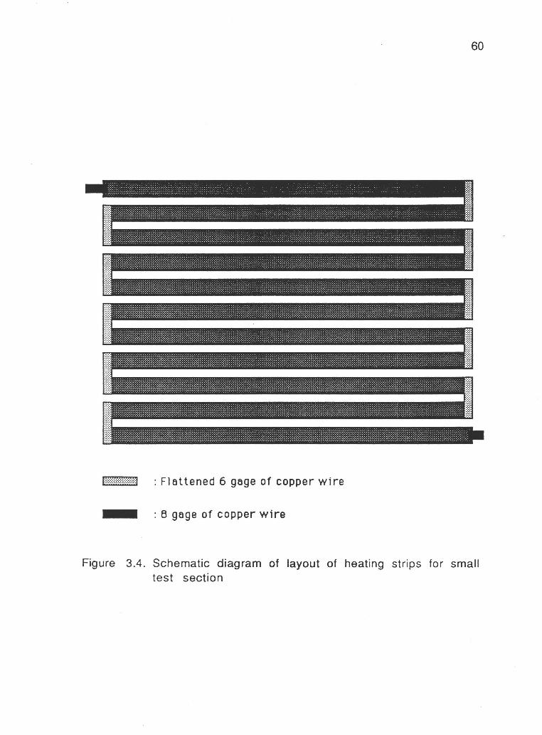
Figures 3.4 and 3.5 show schematic diagrams of the layout of
the heating elements for both test sections.
(2) Construction
Heating elements had to be electrically insulated from the tube
wall. In order to provide good insulation, a 3.5-mil double-coated
polyester film with a rubber-resin adhesive on each side, with a
width of 1.5 inches, was applied in longitudinal strips along the
outside wall of the copper tubes. This tape was specified by the
61
: Flattened 6 gage of copper wire: 8 gage of copper wire
Figure 3.5. Schematic diagram of layout of heating strips for largetest section
62
manufacturer to have a high dielectric strength and capable of
withstanding 130°C. A 1.25-inch width of woven glass tape was
placed longitudinally over the polyester film. The glass tape was
able to withstand temperatures up to 180°C. Using the thermal
conductivities of each material (0.24056 W/m°K for the poly-
esterfilm and 0.16666 W/m°K for the woven glass tape) the
temperature drop across the insulation was estimated to be about
19°C for the maximum heat flux used in the present study.
A formidable effort was required to attach the heating
elements onto the tape while maintaining even spacing. Each strip
was 10-ft long The desired spacing was accomplished after many
trials.
Electrical connections between heating strips were made by
silver-soldering a copper strip across the ends. This process was
repeated until a complete series curcuit was made. Special care
was taken during the soldering to minimize damage to the
insulation.
Precise locations for the thermocouple attachments were
measured and noted on the tape. Then the same polyester film was
wound 2 times around the heating elements. Additional polyimide
film was wound once over the entire tape for a better thermalinsulation. Marks for the thermocouple positions were visible
through this transparent tape.
(3) Other details
Holes were cut in the insulating tape, at desired thermo-
63
couple locations. The insides of the holes were cleaned and the
thermocouples were carefully attached to the bottom wall of the
hole with a paste that was both highly conducting and temperature
resistant. Each thermocouple was also covered with an epoxy for
added strength.
In each test section 24 thermocouples were placed at axial
locations, 3, 9, 18, 30, 48, 68, 91, and 117 inches downstream from
the beginning of the heating section. An additional thermocouple
was mounted at the bottom of the each test section just prior to
the exit. Readings for this location were monitored by the data
acquisition system to establish that the maximum design wall
temperature was maintained. Each thermocouple was at a depth of
30 mils. Three thermocouples were placed on the top, side, and at
the bottom of the tube at each axial position. A relatively low
thermally-conductive epoxy, Omegabond 100, was also used for
permanent bonding of the thermocouple. Additional Omegabond 100
was packed around the exposed thermocouple wires for thorough
insulation from the heating elements. Finally two coats of
polyurethane insulation were sprayed over the entire test section.
Photographs are shown in Figure 3.6 through Figure 3.10, which
show respectively: 1) an overall view of test apparatus, 2) test
sections with heating strips attached, 3) test sections in place
with the loose insulation removed from the enclosure, 4) weigh
tank, feed tank, and pump, 5) entrance sections, heat exchanger, and
static mixer.
64
Figure 3.6. Overall view of test apparatus*
*Numbers in the figure indicate the following:1. weigh tank 2. tank mixer 3. scale 4. entrance sections5. switch boxes 6. power supply 7. ice bath container8. potentiometer 9. standard cell 10. constant voltage supply11. viscometer 12. data acquisition system
65
Figure 3.7. Test sections with heating strips attached
66
Figure 3.8. Test sections with surrounding insulation removed
67
Figure 3.9. View of weigh tank, feed tank, tank mixer, andpump
r r 1
imp
:o t rrt ,Tx..
Figure 3.10 View of entrance sections, heat exchanger, and staticmixer
68
3.2.4 Viscometer
The Viscotester VT500 manufactured by the Haake Company in
West Germany, a kind of rotational viscometer, was used for
evaluating the non-Newtonian character of the test fluids. The
viscosity measurement system consisted of the viscometer, a
tempering vessel, rotors and beaker, a constant temperature
circulator, and a temperature sensor. Its speed range varied from 2
to 500 rpm.
The principle of rotational viscometers is to measure the
resistance of a fluid against the inner cylinder which rotates at a
defined rotational speed while the outer cylinder is held stationary
(Searle system). It develops a Couette flow in the annular gap
between the rotating inner cylinder and stationary concentric outer
cylinder. Figure 3.11 shows a schematic diagram of the rotational
viscometer.
69
Torque sensor
Rotor
Figure 3.11. Schematic diagram of the rotational viscometer
70
Chapter 4. MEASUREMENT SYSTEM
4.1 Temperature measurement
Forty eight wall temperature readings and the inlet and outlet
fluid temperature readings were taken at each operating condition
by means of a potentiometer. Ten additional temperature readings
were recorded using a data acquisition system. This system
consisted of an HP 3421A data acquisition/ control unit, an HP-87
computer, and an HP-IB interface.
Copper-constantan thermocouples insulated with teflon were
used. Appropriate lengths were cut to fit each location of the
measuring site, the potentiometer, the data acquisition system, ice
bath, and switch boxes. Copper-constantan thermocouples were
also used for the other 10 measurement locations including those
for the inlet and outlet fluid temperatures.
Twenty five thermocouples were attached to each test section,
all but one were wired to the potentiometer through the
thermocouple switch boxes and ice bath reference junction. The
other was mounted at the bottom of the wall just prior to the end
of the test section. In order to check the wall temperature and
assure steady state, this one was connected to the 3421A data
acquisition/control unit. A null detector, constant voltage supply,
and standard cell were used in conjunction with the Leeds and
Northrup 7554 type K-4 potentiometer. Figure 4.1 shows a
schematic diagram of the temperature measurement system.
71
Thermocouple probes were used to measure flow temperatures
at 4 locations, these being in the main flow at the outlet of the
feed tank, just prior to the entrance sections, just after the outlet
mixer, and at the inlet to the shell side of the heat exchanger.
Another thermocouple probe was used in an auxilary capacity to
measure the room temperature near the entrance sections.
Five thermocouples were also attached at the following
locations: 6 inches upstream of the inlet on the top of the outside
surface of each entrance section, 1 inch downstream of the last
wall thermocouple on the outside wrap of each test section, and in
the vicinity of the end of the entrance sections.
To verify steady state operation of the flow system, the wall
temperatures at the bottom near the end of the test section, at the
inlet to the entrance section, at the inlet to the heat exchanger, and
on the outside wrap of the test section were continuously checked
using the data acquisition system. The system required less than 2
hours to reach steady state.
4.2 Thermocouple calibration
Calibration of each thermocouple was made using the same
circuit as shown in Figure 4.1 before they were mounted in the
apparatus. They were calibrated using a Fluke 2180A RTD digital
thermometer, the Haake constant temperature circulator, and the
K-4 potentiometer. The maximum error of the thermometer was
±0.1 °C over the temperature range used during the calibration.
Figure 7.22 shows a comparison of the present experimental
results with those of the Bassett and Welty [9] correlation which
does not account for free convection effects. The present data
follow a different slope from their correlation. At the highest
value of Gz (Gz = 27,000) the present results are 9% lower than the
Bassett and Welty prediction, however the present data generally
show higher heat transfer rates up to 42% higher at Gz = 127.
In Figure 7.23 the present heat transfer results are compared
1 1 1
0 Conditions:8j=1 .081
Pr Wi=4932A H/RuT = 5.6X38.6Br-0 0
i
Gz
Figure 7.20. Comparison of experimental results with Cochrane'snumerical solution
Gz
Figure 7.21. Comparison of experimental results with Cochrane'snumerical solution
1 1 2
Gz
Figure 7.22. Comparison with Bassett and Welty results
1 1 3
with a correlation of Mahalingam et al [90] which was obtained
from 23 data points displaying buoyancy effects. The present data
display considerable scatter for Ra evaluated at the wall
temperature. The difference between the present data and their
equation ranged from 3.3% to 35.9%, with the mean deviation being
15.1% below their predicted values.
Figure 7.24 shows a comparison between the present heat
transfer results and those of Joshi [6l X+ < 0.013; our results
show higher heat transfer rates than his. The present heat transfer
rates are 22.1%, 16.3%, 12.3%, 38.7%, and 27.9% higher at X+ =
0.00078, 0.00096, 0.00179, 0.00320, and 0.0109, respectively. X+
indicates a dimensionless distance, 2 (x/D)/(Re Pr) or 7t/(2 Gz).
Excluding 3 runs, which showed noticeable buoyancy effects,
the best correlation for this work was obtained using the
dimensionless parameters,
=Gzb + 0.0083 (Rab)°.75
and
7c2 = Nub (KW /Kb )0.14 . 1 / 3 3
These parameters have been employed to correlate tube flow
data for a Newtonian fluid with free convection effects using the
viscosity ratio, µw /µb, instead of KW /Kb [115]. With this change
they were found to be valid for a non-Newtonian fluid also. A
better correlation was obtained in the present work using Ra
evaluated at bulk flow conditions while Mahalingam et al correlated
1 1 4
10000
Gz + 0.0083 Re75
1 00 0 00
Figure 7.23. Comparison with results of Mahalingam et al
100
Z 0
0 .0001 .001
x+
.01
Figure 7.24. Comparison with Joshi results
1 1 5
116
their 23 data points with Ra evaluated at wall conditions.
Considering radial viscosity variation with temperature, non-
Newtonian effects, both forced and free convection effects, the
correlation obtained in the present study is
, ,..1/3Nub (Kw/Kb)
o .14li/Ow = 2.116 [GZb ± 0.0083 (Rab)0.7510.27 (7.2)
which gave the value of the coefficient of determination, R2, of
0.973 and detailed information on statistical analysis of this
regression fit is included in Appendix I. The present data and their
correlation equation are shown in Figure 7.25.
1 00
loo 1000
Gz + 0.0083 R'75
1 0 0 00
Figure 7.25. Correlation of data from present runs
1 0 0 00 0
1 1 8
Chapter 8. CONCLUSIONS AND RECOMMENDATIONS
This experimental study has provided data for the combined
free and forced convective heat transfer to pseudoplastic fluids in
the thermal entry region of uniformly heated, horizontal pipes.
Viscometric data for the test fluids used were seen to fit the
power-law model. The following conclusions can be drawn:
1. The local rate of combined convective heat transfer for a
fluid with temperature-dependent properties, especially viscosity,
except at high Graetz numbers where buoyancy effects were
relatively small, is greater than equation (7.1) which is a
temperature-independent property solution.
2. The local rate of combined convective heat transfer is
84.5% higher than predicted by the temperature-independent
solution at Gz = 231 for a solution with 5% CMC, and 35% higher
than predicted by the temperature-independent solution at Gz = 140
for a CMC concentration of 8.3 percent.
3. The local rate of combined convective heat transfer of non-
Newtonian fluids where significant free convection effects occur is
greater than for purely forced convection due to their additional
free convection effects caused by secondary flows.
4. Local heat transfer rates are higher than those expressed by
the correlation reported by Bassett and Welty [9], which does not
account for free convection effects. For example results of this
study are 42% higher at a value of Gz = 127.
5. Both temperature-dependent fluid properties and free
1 1 9
convection effects are significant factors on the total heat transfer
rate. Heat transfer rates are increased by as much as 384% for Gzx
= 681 and Rax = 154100 over the classic constant value of 4.364 for
full thermal development. Non-Newtonian effects accounted for by
the term, 81/3,are relatively small.
6. Free convection effects become greater for less viscous
fluids due to their greater buoyancy effects; and this increase
becomes greater as the flow progress downstream.
7. Using estimated values of Ra* and Gz at transition the
parameter Ra*/Gz2 varied from 0.1, for Ra* = 3.20 x 10⁵ and Gz =
2069, to 1.9 for Ra* = 1.84 x 10⁶ and Gz = 981. A value of the ratio,
Ra*/Gz2, near unity appears to be a reasonable estimate as a
transition criterion.
8. The dimensionless parameters, ni =Gzb + 0.0083 (Rab)°75
and 7t2 = Nub (Kw/Kb)014 (1/8w 1 /3) represent the data of this work
well, including combined free- and forced-convection heat transfer
behavior. Equation (7.2) expresses the rate of heat transfer for
flows with temperature-dependent properties, free convection
effects, and non-Newtonian effects .
9. Viscous heating for fluids with Brinkman numbers as high
as 1.7 x 10⁻⁴ did not influence heat transfer rates.
It is recommended that future work address:
1. Experimental investigations with highly-viscous pseudo-
plastic fluids to determine viscous dissipation effects
2. Flow patterns and associated heat transfer behavior for
turbulent flows of pseudoplastic fluids in uniformly-heated
120
horizontal pipes
3. The heat transfer behavior of dilatant fluids and Bingham
plastic fluids in uniformly-heated horizontal pipes
4. The development of alternative techniques to determine the
flow patterns characteristic of secondary flows in pseudoplastic
fluids
121
BIBLIOGRAPHY
Acrivos, A., "A Theoretical Analysis of Laminar NaturalConvection Heat Transfer to Non-Newtonian Fluids," AIChE. J.,Vol. 6, No. 4, 584-590 (1960).
2. Acrivos, A.,"On the Combined Effect of Forced and FreeConvection Heat Transfer in Laminar Boundary Layer Flows,"Chem. Eng. Sci.. Vol. 21, 343-352 (1966).
3. Acrivos, A. and J. D. Goddard, "Asymptotic Expansions forLaminar Forced-Convection Heat and Mass Transfer," J. FluidMech., Vol. 23, 273-291(1965).
4. Acrivos, A., M. J. Shah, and E. E. Petersen, "Momentum and HeatTransfer in Laminar Boundary-Layer Flows of Non-NewtonianFluids Past External Surface," AIChE J., Vol. 6, No. 2, 312-317(1960).
5. Amato, W. S. and C. Tien, "Free Convection Heat Transfer fromIsothermal Spheres in Polymer Solutions," Int. J. Heat MassTransfer., Vol 19, 1257-1266 (1976).
6. Ames, W. F., Nonlinear Partial Differential Equations,Academic Press, New York (1965).
7. Bader, H. J., A. A. Mckillop, and J. C. Harper, "An Experimentaland Analytical Study of Entrance Flow of Non-NewtonianFluids," Heat Transfer 4:Rh1. (1970).
8. Bassett, C. E., "An Experimental Study of Forced ConvectionHeat Transfer to Non-Newtonian Fluids in the Thermal EntranceRegion of a Horizontal, Uniformly Heated, Circular Pipe," Ph.D.Thesis, Oregon State University, Corvallis (1975).
9. Bassett, C. E., and J. R. Welty, "Non-Newtonian Heat Transfer inthe Thermal Entrance Region of Uniformly, Heated, Horizontalpipes," AIChE J., Vol. 21, No. 4, 699-706 (1975).
122
10. Berg les, A. E. and R. R. Simonds, "Combined Forced and FreeConvection for Laminar Flow in Horizonal Tubes with UniformHeat Flux," Int. J Heat Mass Transfer, Vol. 14, 1989-2000(1971).
11. Berkowski, B. M., "A Class of Self-Similar Boundary LayerProblems for Rheological Power-Law Fluids," Int. Chem. Eng.,Vol. 6, No. 2, 187-201 (1966).
12. Bird, R. B., "Zur Theorie des Warmeubergangs an Nicht-Newtonsche Flussigkeiten bei Laminarer Rohrstromung,"Chemie.-Ingenieur.- Technik., Vol. 31, 569-572 (1959).
13. Bird, R. B., R. C. Armstrong, and 0. Hassager, Dynamics ofPolymeric liquid, Vol. I, Wiley, New York (1977).
14. Brown, A. R. and M. A. Thomas, "Combined Free and ForcedConvection Heat Transfer for Laminar Flow in HorizontalTubes," J. Mech. Eng. Sci., Vol. 7, 440-448 (1965).
15. Chang, T. A., D. R. Jeng, and K. J. Dewitt, "Natural Convectiion toPower-Law Fluids from Two-Dimensional or AxisymmetricBodies of Arbitrary Contour," Int. J Heat Mass Transfer, Vol.31, No. 3, 615-624 (1988).
16. Campo, A. and C. Schuler, "Heat Transfer in Laminar Flowthrough Circular Tubes Accounting for Two-Dimensional WallConduction," Int. J Heat Mass Transfer. Vol. 31, No. 11, 2251-2259 (1988).
17. Charm, S. E. and E. W. Merrill, "Heat Transfer Coefficients inStraight Tubes for Pseudoplastic Food Materials in StreamlineFlow," Food Research, Vol. 24, 319-331 (1959).
18. Chen and Wollersheim, "Free Convection at a Vertical Platewith Uniform Flux Condition in Non-Newtonian Power-LawFluids," J. Heat Transfer, Vol 95, 123-124 (1973).
19. Cheng, K. C. and J. W. Ou, "Free Convection Effects on Graetz
123
Problem for Large Prandtl Number Fluids in Horizontal Tubeswith Uniform Wall Heat Flux," Proceedings of the Fifth Int. J.Heat Transfer Conference, Vol. 3, 159-163 (1977).
20. Cho, Y. I. and J. P. Hartnett, "Non-Newtonian Fluids in CircularPipe Flow," Adv. Heat Transfer, 59-141 (1982).
21. Christiansen, E. B. and G. E. Jensen, "Energy Transfer to Non-Newtonian Fluids in Laminar Flow," Progress in InternationalResearch on Thermodynamic and Transport Properties, ed. by J.F. Masi and Tsai, New York, Academic Press, 738-747 (1962).
22. Christiansen, E. B. and S. E. Craig, "Heat Transfer to Pseudo-plastic Fluids in Laminar Flow," AIChE J., Vol. 8, 154-160(1962).
23. Christiansen, E. B., S. E. Craig, and T. R. Carter, "The Effect ofTemperature on The Consistency of Fluids," Trans. Soc. Rheol,Vol. 10, No. 1, 419-430 (1966).
24. Churchill, S. W., "A Comprehensive Correlating Equation forLaminar, Assisting, Forced and Free Convection," AIChE J., Vol23, 10-16 (1977).
25. Cochrane, G. F., "A Numerical Solution for Heat Transfer toNon-Newtonian Fluids with Temperature-Dependent Viscosityfor Arbitrary Conditions of Heat Flux and SurfaceTemperature," Ph.D. Thesis, Oregon State Univ., Corvallis(1969).
26. Cochrane, G. F., "Cooling of Newtonian and Non-NewtonianFluids with Temperature-Dependent Viscosity," Albuquerque,1972. 13 numb.leaves. (University of New Mexico. College ofEngineering. Bureau of Engineering Research. Technical ReportME-61 (71) SAN-183-2 on Sandia contract 51-0059, task 2).
27. Colburn, A. P. "A Method of Correlating Forced Convection HeatTransfer Data and a Comparison with Fluid Friction," Trans. ofAIChE, Vol. 29, 174 (1933).
124
28. Collins, E. A. and F. E. Filisko, "Temperature Profiles forPolymer Melts in Tube Flow," AIChE J., Vol. 16, No. 3, 339-344(1970).
29. Coutier, J. P. and R. Greif, "An Investigation of Laminar MixedConvection Inside a Horizontal Tube with Isothermal WallConditions," Int. J. Heat Mass Transfer, Vol. 28, No. 7, 1293-1305 (1985).
30. Dale, J. D., "Laminar Free Convection of Non-Newtonian Fluidsfrom a Vertical Flat Plate with Uniform Surface Heat Flux,"Ph. D. Thesis, University of Washington, Seat le (1969).
31. Dale, J. D. and A. F. Emery, "The Free Convection of Heat from aVertical Plate to Several Non-Newtonian PseudoplasticFluids," J. Heat Transfer, Vol. 94, 64-72 (1972).
32. De young, S. H.and G. F. Scheele, "Natural Convection DistortedNon-Newtonian Flow in a Vertical Pipe," AIChE J., Vol. 16,712-717 (1970).
33. Del Casal, E., and W. N. Gill, A Note on Natural ConvectionEffects in Fully Developed Horizontal Tube Flow," AIChE J., Vol.8, 570-574 (1962).
34. Denn, M. M., "Boundary Layer Flows for a Class of ElasticFluids," Chem. Eng. Sci., Vol. 22, No.3, 395-405 (1967).
35. Depew C. A., J. L. Franklin, and C. H. Ito, Combined Free andForced Convection in Horizontal, Uniformly Heated Tubes,"ASME Paper No. 75-HT-17 (1975).
36. Depew, C. A. and S. E. August, "Heat Transfer Due To CombinedFree and Forced Convection in a Horizontal and IsothermalTube," Trans, ASME. Series C. J. Heat Transfer, Vol 93, 380-384 (1971).
37. Dodge, D. W. and A. B. Metzner, "Turbulent Flow of Non-Newtonian Fluids," AICHE J., Vol. 5, 189-204 (1959).
125
38. Etchart, D. Y. "A Pipe Entry Length Solution for Heat Transferand Flow in Powell-Eyring Fluids with Temperature-DependentViscosity and Constant Flux Boundary Condition," M.S. Thesis,Corvallis, Oregon State University (1971)
39. Etchart, D. Y. and J. R. Welty, "Numerical Solution for HeatTransfer and Pressure Drop for Pseudoplastic Fluids in LaminarPipe Flow with Constant Wall Heat Flux," AICHE 17th NationalHeat Transfer Conference, Heat Transfer and Energy ConversionDivision, 59-68 (1977).
40. Eubank, C. C. and W. S. Procter, "Effect of Natural Convection onHeat Transfer with Laminar Flow in Tubes," M.S. Thesis,Massachussetts Institute of Technology (1951).
41. Faris, G. N. and R. Viskanta, "An Analysis of Laminar CombinedForced and Free Convection Heat Transfer in a Hoizontal Tube,"Int.J. Heat Mass Transfer, Vol 12, 1295-1309 (1969).
42. Foraboschi, F. P. and I. de Federico, "Heat Transfer in LaminarFlow of Non-Newtonian Heat-Generating Fluids," Int. J. HeatMass Transfer, Vol. 7, 315-325 (1964).
43. Forrest, G. and W. L. Wilkinson, "Laminar Heat Transfer toTempeature-Dependent Bingham Fluids in Tubes," Int. J. HeatMass Transfer, Vol. 16, 2377-2391 (1973).
44. Forsyth, T. H. and N. F. Murphy, "Temperature Profiles of MoltenFlowing Polymers in a Heat Exchanger," AICHE J., Vol. 15, 758-763 (1969).
45. Friend, W. L. and A. B. Metzner, "Turbulent Heat Transfer InsideTubes and The Analogy Among Heat, Mass, and MomentumTransfer," AICHE J., Vol.4, 393-402 (1958)
46. Gee, R. E. and J. B. Lyon, "Nonisothermal Flow of Viscous Non-Newtonian Fluids," Ind. Eng. chem., Vol. 49, 956-960 (1957).
47. Gentry, C. C. and D. E. Wollersheim, "Local Free Convection toNon-Newtonian Fluids from a Horizontal Isothermal Cylinder,"
126
J. Heat Transfer, Vol 96, 3-8 (1974).
48. Gill, W. N., "Heat Transfer in Laminar Power Law Flows withEnergy Source," AIChE J., Vol. 8, 137-138 (1962).
49. Gottifredi, J. C., et al., "Heat Transfer To Newtonian and Non-Newtonian Fluids Flowing In A Laminar Regime," Int. J. HeatMass Transfer, Vol. 26, No.8, 1215-1220 (1983).
50. Graetz, L., "Lieber die warmeleitungsfahigkeit von flussig-keiten," Ann. Physik Chemie, Vol. 25, 337-357 (1885).
51. Griskey, R. G. and I. A. Wiehe, "Heat Transfer to Molten FlowingPolymer," AICHE J., Vol. 12, 308-312 (1966).
52. Halmos, A. L. and D. V. Boger, "Flow of Viscoelastic PolymerSolutions Through an Abrupt 2-to-1 Expansion," Tran. of theSociety of Rhea logy, Vol. 20(2), 253-264 (1976).
53. Han, C. D., M. Charles, and W. Philippoff, "Measurement of theAxial Pressure Distribution of Molten Polymers in FlowThrough a Circular Tube," Trans. the Society of Rheoloay, Vol.13(4), 455-466 (1969).
54. Hanks, R. W. and E. B. Christiansen, "The laminar nonisothermalflow of non-Newtonian fluids," AICHE J., Vol. 7, 519-523(1961).
55. Hartnett, J. P. and E. Y. Kwack, "Prediction of Friction and HeatTransfer for Viscoelastic Fluids in Turbulent Pipe Flow,"Reprinted from Int. J. of Thermophysics, Vol. 7, No. 1, 53-63(1986)
56. Hartnett, J. P., E. Y. Kwack, and B. K. Rao, "HydrodynamicBehavior of Non-Newtonian Fluids in a Square Duct,"Rheology, 30(s), S45-S59 (1986).
57. Hartnett, J. P. and M. Kostic, "Heat Transfer to a ViscoelasticFluid in a Laminar Flow through a Rectangular Channel," Int. J.
127
Heat Mass Transfer, Vol. 28, No. 6, 1147-1155 (1985).
58. Hieber, C. A., "Laminar Mixed Convection in an Isothermal Tube:Correlation of Heat Transfer Data," Int. J. Heat Mass Transfer,Vol. 25, 1737-1746 (1982).
59. Hieber, C. A., "Mixed convection in an Isothermal HorizontalTube: Some Recent Theories," Int. J. Heat Mass Transfer, Vol.24, 315-322 (1981).
60. Hieber, C. A. and S. K. Sreenivasan, "Mixed Convection inIsothermally Heated Horizontal Pipe," Int. J. Heat MassTransfer, Vol. 17, 1337-1348 (1974).
61. Hishida, M., Y. Nagano, and M. S. Montesclaros, Combined Forcedand Free Convection in the Entrance Region of an IsothermallyHeated Horizontal Pipe," J. Heat Transfer, Vol. 104, 153-159(1982)
62. Hong, S. W., S. M. Morcos, and Berg les A. E., Analytical andExperimental Results for Combined Forced and Free LaminarConvection in Horizontal Tubes," Proceedings of the Fifth Int.Heat Transfer Conference, Vol. 3, 154-158 (1974).
63. Hussain, N. A. and S. T. McComas, "Experimental Investigationof Combined Convection in a Horizontal Circular Tube withUniform Heat Flux," Heat Transfer 1970, Vol. 4, NC 3.4 (1970).
64. Hwang, G. J. and K. C. Cheng, "Boundary Vorticity Method forConvective Heat Transfer with Secondary Flow - Application tothe Combined Free and Foeced Convection in Horizontal Tubes,"Heat Transfer 1970, Vol. 4, Paper No. NC 3.5, ElsevierPublishing Co., Amsterdam (1970).
65. Inman, R. M., "Heat transfer to Laminar Non-Newtonian Flow ina Circular Tube with Variable Circumferential WallTemperature or Heat Flux," Cleveland, Ohio, 1965 22p. (U.S.National Aeronaautics and Space Administration, TechnicalNote D-2674)
128
66. Jackson, T. W., J. M. Spur lock, and K. R. Purdy, "Combined Freeand Forced Convection in a Constant Temperature HorizontalTube, " AIChE J., Vol. 7, 38-45 (1961)
67. Joshi, S. D. and A. E. Berg les, "Experimental Study of LaminarT..kn CIntAi of KInn_KlatAftnnian Ph " .1
Erratum67* Joshi, S. D., "Heat Transfer in In-Tube Flow of Non-Newtonian
Fluids," Ph.D. Thesis, Ames, Iowa State University (1978).
69. Khabakhpasheva, E. M., V. I. Popov, and B. V. Perepelitsa, "HeatTransfer in Viscoelastic Fluids," Heat Transfer 4:Rh2 (1970).
70. Kim, C. B. and D. E. Wollersheim, Free Convection Heat Transferto Non-Newtonian, Dilatant Fluids from a Horizontal Cylinder,"J. Heat Transfer, Vol. 98, 144-148 (1976).
71. Kleppe, J. and W. J. Marner, "Transient Free Convection in aBingham Plastic on a Vertical Flat Plate," J. Heat Transfer,Vol. 94, 371-376 (1972).
72. Korayem, A. Y., "Non- Isothermal Lamianr Flow of Non-Newtonian Fluids in the Entrance Region of a Pipe," Ph. D.Thesis. Davis, California, Univ. of California at Davis, 1964.121 numb. leaves.
73. Knudsen, J. G. and D. L. Katz, Fluid Dynamics and Heat Transfer,Robert E. Krieger Publishing Company, Hungtington, New York(1979).
74. Krantz, W. B. and D. T. Wasan, "Heat, Mass, and MomentumTransfer Analogies for the Fully Developed Turbulent Flow ofPower Law Fluids in Circular Tubes," AICHE J., Vol. 17, 1360-1367 (1971).
75. Kubair, V. G. and D. C. Pei, "Combined Laminar Free and ForcedConvection Heat Transfer to Non-Newtonian Fluids," Int. J. Heat
129
Mass Transfer, Vol. 11, 855-869 (1968).
76. Kumar, R., "Heat Transfer in Laminar Flow of Bingham MaterialThrough a Circular Pipe," Appl. Sci. Res., Sect. A, Vol. 15, 87-96 (1965).
77. Kupper, A., E. G. Hauptmann and M. lqbal, "Combined Free andForced Convection in a Horizontal Tube under Uniform HeatFlux," Solar Energy, Vol. 12, 439-446 (1969).
78. Kutateladze, S. S., et al., "Hydraulic Resistance and HeatTransfer in Stabilized Flow of Non-Newtonian Fluids," HeatTransfer - Soviet Research, Vol. 2(6), 114-123 (1970).
79. Lakshminarayanan, M. S., R. Lalchanpani, and M. R. Rao,"Turbulent Flow Heat Transfer to Non-Newtonian Fluids inCircular Tubes," Indian J. Technology, Vol. 14, 521-525 (1976).
80. Lee, S. Y. and W. F. Ames, "Similarity Solutions for Non-Newtonian Fluids," AICHE J., Vol. 12, NO. 4, 700-708 (1966).
81. Lee, W. Y., Y. I. Cho, and J. P. Hartnett, "Thermal ConductivityMeasurements of Non-Newtonian Fluids," Lett Heat MassTransfer, Vol. 8, 255-259 (1981).
82. Leveque, J., Anna les des Mines, Ser. 12, 13:201, 305 and 381(1928).
83. Lichtarowicz, A., "Combined Free and Forced ConvectionEffects in Fully Developed Laminar Flow in Horizontal Tubes,"Heat and Mass Transfer by Combined Forced and FreeConvection, Institute of Mechanical Engineers. London, 13-16(1972).
84. Lin, H. T. and Y. P. Shih, "Combined Laminar Free and ForcedConvection from A Vertical Plate to Power Law Fluids," Chem.Eng. Comm., Vol. 7, 327-334 (1980).
85. Lin, H. T. and Y. P. Shih, "Laminar Boundary Layer Heat Transfer
130
to Power-Law Fluids," Chem. Eng. Comm., Vol 4, 557-562(1980).
86. Lloyd, J.R. and E. M. Sparrow,"Combined Forced and FreeConvection Flow on Vertical Surfaces," Int. J. Heat MassTransfer. Vol. 13, 434-438(1970).
87. Lyche, B. C. and R. B. Bird, "The Graetz-Nusselt Problem for aPower-Law Non-Newtonian Fluid," Chem. Eng. Sci., Vol. 6, 35-41 (1956).
88. Lyons, D. W., J. W. White, and J. D. Hatcher, "Laminar NaturalConvection Heat Transfer in Dilute Aqueous PolymerSolutions," Ind. Eng. Chem. Fundam., Vol. 11, 586-588 (1972).
89. Lyon, R. N., "Liquid Metal Heat Transfer Coefficients," Chem.Eng. Progr. Symo. Ser. No. 2, 47, 75-79 (1951).
90. Mahalingam, R., L. 0. Tilton, and J. M. Coulson, Heat Transfer inLaminar Flow of Non-Newtonian Fluids," Che. Eng. Sci.,Vol. 30,921-929 (1975).
91. Marner, W. J. and H. Hovland, "Viscous Dissipation Effects inFully Developed Combined Free and Forced Non-NewtonianConvection in a Vertical Tube," Warme- and Stoffubertragung,Vol. 6, No. 4, 199-204 (1973).
92. Marner, W. J. and H. K. McMillan, "Combined Free and ForcedLaminar Non-Newtonian Convection in a Vertical Tube withConstant Wall Temperature," Chem. Eng. Sci.. Vol. 27, 473-488(1972).
93. Marner, W. J. and R. A. Rehfuss, "Buoyancy Effects on FullyDeveloped Non-Newtonian Flow in a Vertical Tube," The Chem.Eng. J., Vol. 3, 294-300 (1972).
.94 Matsuhisa, S. and R. B. Bird, "Analytical and NumericalSolutions for Laminar Flow of the Non-Newtonian Ellis Fluid,"AICHE J., Vol. 11, 588-595 (1965).
131
95. McComas, S. T. and E. R. G. Eckert, Combined Free and ForcedConvection in a Horizontal Circular Tube," J. Heat Transfer,Trans. ASME, Series C, Vol. 88, 147-153 (1966).
96. McKiliop, A. A., "Heat Transfer for Laminar Flow of Non-Newtonian Fluids in Entrance Region of a Tube," Int. J. HeatMass Transfer, Vol. 7, 853-862 (1964).
97. Mena, B., G. Best, P. Bautista, and T. Sanchez, "Heat Transfer inNon-Newtonian Flow through Pipes," Rheol. Acta 17, 455-457(1978).
98. Metzner, A. B., "Heat Transfer in Non-Newtonian Fluids," Adv.Heat Transfer, Vol. 2, 357-397 (1965).
99. Metzner, A. B. and P.S. Friend, "Heat Transfer to Turbulent Non-Newtonian Fluids," Ind. Eng. Chem., Vol. 51, 879-882 (1959).
100. Metzner, A. B. and D. F. Gluck, Heat Transfer to Non-NewtonianFluids under Laminar-Flow Conditions," Chem. Eng. Sci., Vol.12, 185-190 (1960).
101. Michiyoshi, I., "Heat Transfer of Slurry Flow with Internal HeatGeneration," Bull. JSME, Vol. 5, 315-319 (1962).
102. Michiyoshi, I. and R. Matsumoto, "Heat Transfer of Slurry Flowwith Internal Heat Generation," Bull. JSME, Vol. 7, 376-384(1964).
103. Michiyoshi, I., R. Matsumoto, and M. Hozumi, "Heat Transfer ofSlurry Flow with Heat Generation, Bull. JSME, Vol.6, 496-504(1963).
104. Mitsuishi, N. and 0. Miyatake, "Laminar Heat Transfer to Non-Newtonian Ellis Model Fluids in Cylindrical Tubes," Chem. Eng.Japan, Vol. 5, 82-86 (1967).
105. Mitsuishi, N. and 0. Miyatake, "Heat Transfer of Non-NewtonianLaminar Flow in Tubes with Constant Wall Heat Flux," Kagaku
132
Kogaku, Vol. 32, 1222-1227 (1968).
106. Mitsuishi, N. and 0. Miyatake, "Heat Transfer with Non-Newtonian Laminar Flow in a Tube Having a Constant Wall HeatFlux," Int. Chem. Eng., Vol. 9, 352-357 (1969).
107. Mizushina, T., et al., "Laminar Heat Transfer to Non-NewtonianFluids in a Circular Tube (Constant Heat Flux)," Kagaku Kogaku,Vol. 31, 250-255 (1967).
108. Morcos, S. M. and A. E. Berg les, "Experimental Investigation ofCombined Forced and Free Laminar Convection in HorizontalTubes," ASME J. Heat Transfer, Vol. 97, 212-219 (1975).
109. Mori, Y., K. Futagami, S. Tokuda, and M. Nakamura, "ForcedConvective Heat Transfer in Uniformly Heated Horizontal Tubes- 1st report: Experimental Study on the Effect of Buoyancy,"Int. J. Heat Mass Transfer, Vol. 9, 453-463 (1966).
110. Morton, B. R., "Laminar Convection in Uniformlyl HeatedHorizontal Pipes at Low Rayleigh Numbers," Quart. J. Mech.Appl. Math., Vol. 12, 410-422 (1959).
111. Na, T. Y. and A. G. Hansen, "Possible Similarity Solutions of theLaminar Natural Nonvection Flow of Non-Newtonian Fluids,"Int. J. Heat Mass Transfer, Vol. 9, NO. 3, 261-262 (1966).
112. Newell, P. H., Jr. and A. E. Berg les, "Analysis of Combined Freeand Forced Convection for Fully Developed Laminar Flow inHorizontal Tubes," ASME J. Heat Transfer, Vol. 92, 83-89(1970).
113. Ng, M. L. and J. P. Hartnett, "Natural Convection in Power LawFluids," Int. Commun. Heat Mass Transfer, Vol. 13, No. 1, 115-120 (1986).
114. Ng, M. L. and J. P. Hartnett, "Free Convection Heat Transfer fromHorizontal Wires to Pseudoplasatic Fluids," Int. J. HeatTransfer, Vol. 31, No. 2, 441-447 (1988).
133
115. Oliver, D. R., "The Effect of Natural Convection on Viscous FlowHeat Transfer in Horizontal Tubes," Chem. Eng Sci., Vol. 17,335-350 (1962).
116. Oliver, D. R., "Non-Newtonian Heat Transfer: an InterestingEffect Observed in Noncircular Tubes," Trans. Inst. Chem. Engrs,Vol. 47, T18-T20 (1969)
117. Oliver, D. R. and R. B. Karim, "Laminar Flow Non-Newtonian HeatTransfer in Flattened Tubes," Can. J. Chem. Eng., Vol. 49, 236-240 (1971).
118. Oliver, D. R. and V. G. Jenson, "Heat Transfer to PseudoplasticFluids in Laminar Flow in Horizontal Tubes," Chem. Eng. Sci.,Vol. 19, 115-129 (1964).
119. Orr, C. and J. M. Dallavalle, "Heat Transfer Properties ofLiquid-Solid Suspensions," Chem. Eng. Prog., Ser. 9, Vol. 50,29-45 (1954).
120. Ou, J. W. and K. C. Cheng, "Natural Convection Effects on GraetzProblem in Horizontal Isothermal Tubes," Int. J. Heat MassTransfer, Vol. 20, 953-960 (1977).
121. Ozoe, H. and S. W. Churchill, "Hydrodynamic Stability andNatural Convection in Ostwald-de Waele and Ellis Fluids: TheDevelopment of a Numerical Solution," AICHE J., Vol. 18,1196-1207 (1972).
122. Parmentier, E. M., "A Study of Thermal Convection in Non-Newtonian Fluds," J. Fluid Mech., Vol. 84, Part 1, 1-11 (1978).
123. Parmentier, E. M., D. L. Turcotte, and K. E. Torrance, "Studies ofFinite Amplitude Non-Newtonian Thermal Convection withApplication to Convection in the Earth's Mantle," J. Geophy.Res., Vol 81, 1839-1846 (1976).
124. Pattison, D. A. "Motionless inline mixers stir up broadinterest," Chemical Engineering, 94-96 (May 19, 1969).
134
125. Pawlek, R. A. and C. Tien, "Laminar Heat Transfer to Non-Newtonian Fluids in Entrance Region of Circular Conduit," Can.J. Chem. Eng., Vol. 42, 222 (1964).
126. Payvar, P., "Asymptotic Nusselt Numbers for Dissipative Non-Newtonian Flow Through Ducts," Appl. Sci. Res., Vol. 27, 297-306 (1973).
127. Petukhov, B. S. and A. F. Polyakov, "Experimental investigationof heat traansfer during viscous gravitational flow of liquid inhorizontal pipe," Teplofizika Vysokikh Temperature, Vol. 5,87-95 (1967)
128. Petukhov, B. S. and A. F. Polyakov, "Effect of Free Convection onHeat Transfer during Forced Flow in Horizontal Pipe,"Teplofizika Vysokikh Temperature, Vol. 5, 348-351 (1967).
129. Pierre, C. St. and C. Tien, "Experimental Investigation ofNatural Convection Heat Transfer in Confined Space for Non-Newtonian Fluid," Can. J. Chem. Eng., Vol. 41, 122-127 (1963).
130. Pigford, R. L., "Nonisothermal Flow and Heat Transfer InsideVertical Tubes," Chem. Eng. Progr. Symp., Ser.No. 17, Vol. 51,79-92 (1955).
131. Reilly, I. G., C. Tien, and M. Adelman, "Experimental Study ofNatural Convection Heat Transfer from a Vertical Plate in aNon-Newtonian Fluid," Can. J. Chem. Eng., Vol. 43, 157-160(1965).
132. Ruckenstein, E., "Interpolating Equations Between Two LimitingCases for the Heat Transfer Coefficient," AICHE J., Vol. 24,940-941 (1978).
133. Schechter, R. S., "On the Steady Flow of a Non-Newtonian Fluidin Non-Circular Tubes," paper presented at the 43rd AIChENational meeting at Tulsa, Okla., Sept. 25-28 (1960).
134. Schenk, J. and J. Van Laar, "Heat Transfer in Non-NewtonianLaminar Flow in Tubes," Appl. Sci. Res., Sec. A., Vol. 7, 449-462
136. Schowalter, W. R., "The Application of Boundary-Layer Theoryto Power-Law Pseudoplastic Fluids: Similar Solutions," AICHE
Vol. 6, No. 1, 24-28 (1960).
137. Seider, E. N. and G. E. Tate, "Heat Transfer and Pressure Drop ofLiquids in Tubes," Industrial and Engineering Chemistry, Vol28, 1429-1436 (1936)
138. Sellars, J. R., M. Tribus, and S. J. Klein, "Heat Transfer toLaminar Flow in a Round Tube or Flat Conduit-the GraetzProblem Extended," Trans. ASME, Vol. 78, 441-448 (1956).
139. Sestak, J. and M. E. Charles, "Limiting Values of Nusselt Numberfor Heat Transfer to Pipeline Flow of Non-Newtonian Fluidswith Arbitrary Internal Heat Generation," Chem. Eng. Progr.Symp. Ser. No. 82, 64, 212-218 (1968).
140. Shannon, R. L., and C. A. Depew, "Combined Forced and Free andForced Convection Laminar Convection in a Horizontal Tubewith Uniform Heat Flux," J. Heat Transfer,Trans. ASME, SeriesC, Vol. 90, 353-357 (1968).
141. Shannon, R. L., and C. A. Depew, "Forced Laminar FlowConvection in a Horizontal Tube with Variable Viscosity andFree-Convection Effects," J. Heat Transfer, Trans. ASME, SeriesC, Vol. 91, 251-258 (1969).
142. Shenoy, A. V., "Natural Convection Heat Transfer to Non-Newtonian Fluids: Studies in The External Flow of Inelastic andViscoelastic Fluids under Laminar and Turbulent conditions,"Ph. D. Thesis, University of Salford, U. K. (1977).
143. Shenoy, A. V., "A Correlating Equation for Combined LaminarForced and Free Convection Heat Transfer to Power-Law
136
Fluids," AICHE J., Vol. 26, 505-507 (1980).
144. Shenoy, A. V., "Combined Laminar Forced and Free ConvectionHeat Transfer to Viscoelastic Fluids," AICHE J., Vol. 26, 683-686 (1980).
145. Shenoy, A. V. and J. J. Ulbrecht, "Temperature Profiles forLaminar Natural Convection Flow of Dilute Polymer Solutionspast an Isothermal Vertical Flat Plate," Chem. Eng.Commun.,Vol. 3, 303-324 (1979).
146. Shenoy, A. V. and R. A. Mashelkar, "Laminar Natural ConvectionHeat Transfer to a Viscoelastic Fluid," Chem. Eng. Sci,, Vol. 33,769-776 (1978).
147. Shenoy, A. V. and R. A. Mashelkar, "Thermal Convection in Non-Newtonian Fluids," Adv. Heat Transfer, Vol. 15, 143-224(1982).
148. Shul'man, Z. P., V. M. Gorislavets, V. A. Rozhkov, and V. V.Uryadova, "Convective Heat Transfer to a Non-LinearViscoplastic Medium in a Circular Tube Allowing forDissipation," Int. Chem. Eng., Vol. 11, No. 2, 325-331 (1971).
149. Siegel, R., E. M. Sparrow, and T. M. Hallman, "Steady LaminarHeat Transfer in a Circular Tube with Prescribed Wall HeatFlux," Appl. Sci. Res., Sec. A, 7, 386-392 (1958).
150. Siegwarth, D. P. and T. J. hanratty, "Computational andExperimental Study of the Effect of Secondary Flow on theTemperature Field and Primary Flow in a Heated HorizonalTube," Int. J. Heat Mass Transfer, Vol. 13, 27-42 (1970).
151. Siegwarth., D. P., R. D. Mikesell, T. C. Readal, and T. J. Hanratty,"Effect of Secondary Flow on the Temperature Field andPrimary Flow in a Heated Horizontal Tube," Int. J. Heat MassTransfer, Vol. 12, 1535-1552 (1969).
152. Skelland, A. H. P., Non-Newtonian flow and heat transfer,Wiley, New York (1967).
137
153. Sparrow, E. M., R. Eichhorn, and J. L. Gregg, "Combined Forcedand Free Convection in a Boundary Layer Flow," Phys. of Fluids.Vol. 2, 319-328 (1959).
154. Tachibana, M., N. Kawabata, and H. Genno, "Steady Laminar Flowof Power-Law Fluids in the Inlet Region of Rectangular Ducts,"J. Rheology, Vol. 30, No. 3, 517-538 (1986).
155. Tien, C., "Laminar Natural Convection Heat Transfer fromVertical Plate to Power-Law Fluid," Appl. Sci. Res.. Vol. 17,233-248 (1967).
156. Tien, C., "The Extension of Couette Flow Solution to Non-Newtonian Fluid," Can. J. Chem. Eng., Vol. 39, 45 (1961).
157. Tien, C., Laminar Heat Transfer of Power-Law Non-Newtonianfluid The Extension of Graetz-Nusselt Problem," Can. J. Chem.Eng., Vol. 40, 130-134 (1962).
158. Tien, C., H. S. Tsuei, and Z. S. Sun, "Thermal Instability of aHorizontal Layer of Non-Newtonian Fluid Heated From Below,"Int. J. Heat Mass Transfer, Vol. 12, 1173-1178 (1969).
159. Tsuei, H. S. and C. Tien, "Free Convection Heated Transfer inHorizontal Layer of Non-Newtonian Fluid," Can. J. Chem. Eng.,Vol. 51, 249-251 (1973).
160. Van Wazer, J. R., et al, "Viscosity and Flow Measurements.", Alaboratory handbook of rheology, New York, Interscience, 58-59 (1963).
161. Vlachopoulos, J. and C. K. John Keung, "Heated Transfer to aPower-Law Fluid Flowing Between Parallel Plates," AICHE J.,Vol. 18, 1272-1274 (1972).
162. Wang, T. Y. and C. Kleinstreuer, "Combined Free-ForcedConvection Heat Transfer between Vertical Slender Cylindersand Power-Law Fluids," Int. Heat Mass Transfer, Vol. 31, No. 1,91-98 (1988).
138
163. Welty, J. R., C. E. Wicks, and R. E. Wilson, Fundamentals ofMomentum. Heat. and Mass Transfer, 3rd edition, John Wiley &Sons.
164. Whiteman, I. R. and D. B. Drake, "Heat Transfer to Flow in aRound Tube With Arbitrary Velocity Distribution," Tran. ASME,Vol. 80, 728-732 (1958).
165. Wissler, E. H. and R. S. Schechter, "The Gretz-Nusselt Problem(with Extension) For a Bingham Plastic," Che. Eng. Pro.g. symp.,Ser. 29, Vol. 55, 203-208 (1959).
166. Yamanaka, A. and N. Mitsuishi, "An Experimental Study onCombined Forced and Natural Convective Heat Transfer fromSpheres to Power-Law Fluids," H. T. Jpn. Res., Vol. 6, No. 4, 85-91 (1977).
167. Yao, L. S., "Entry Flow in Heated Straight Tube," ASME, J. FluidMechanics, Vol. 88, 465-483 (1978).
168. Yao, L. S., "Free-Forced Convection in the Entry Region ofHeated Straight Pipe," ASME, J. Heat Transfer, Vol. 100, 212-219 (1978).
169. Yousef, W.W. and J.D. Tarasuk, "Free Convection Effects onLaminar Forced Convection Heat Transfer in a HorizontalIsothermal Tube," J. Heat Transfer, Vol. 104, 145-152 (1982).
APPENDICES
139
APPENDIX A. Error analysis
140
ANALYSIS OF ERROR
This section includes the estimates for errors in measured
data and dimensionless parameters used in the present work.
For the case when Y is a given function of independent
variables X1, X2, X3,...,Xn; Wy is the uncertainty interval for the
quantity, Y; and W1, W2, W3,...,Wn are the uncertainty intervals for
the independent variables; if the uncertainties in the independent
variables are all given with the same odds, then WY is given as
2 2 -Ny 2 (W7 = ( W (kW3)ax, 1 ax2 2 3 wn) (A.1)
where Y = f(X1 ,X2,X3,...,Xn) and the independent variables X1, X2,
X3,..Xn are measured quantities. If Y is comprised of products and
quotients of the measured variables, then the following equation is
obtained from equation (A.1):
2 2WY N1S/3( Wy2 Wv'3 WXn
Y = 1 +
X2x2 2
2 A .n.2 31 X, (A.2)
The uncertainties from various sources for the basic
quantities used in generating the results in this thesis are shown in
Table A.1. The smallest value measured for the quantity is shown in
the last column. Entries under "Uncertainties other sources" are
as expressed by Bassett [8], and were obtained under the assumption
that fluid properties other than viscosity were equal to those of
thermocouple emf, Etc thermocouple emf, Mf - mass offluid weighed, tf - time for Mf to flow, Tv -viscometertemperature, Tq torque value of the viscometer.
pure water.
Power input to the heaters was directly related to shunt
voltage, shunt resistance, and heater resistance. It was determined
by2
VsP = () Rh
Rs (A.3)
142
An additional uncertainty (4.72%) in the power supplied to the fluid
resulted from heat losses to the enclosure. Thus, the square of the