The Pennsylvania State University The Graduate School College of Engineering AN EXPERIMENTAL STUDY OF FLAME RESPONSE MECHANISMS IN A LEAN-PREMIXED GAS TURBINE COMBUSTOR A Dissertation in Mechanical Engineering by Stephen Peluso Submitted in Partial Fulfillment of the Requirements for the Degree of Doctor of Philosophy August 2012
Transcript
The Pennsylvania State University
The Graduate School
College of Engineering
AN EXPERIMENTAL STUDY OF FLAME RESPONSE MECHANISMS IN A
LEAN-PREMIXED GAS TURBINE COMBUSTOR
A Dissertation in
Mechanical Engineering
by
Stephen Peluso
Submitted in Partial Fulfillment of the Requirements
for the Degree of
Doctor of Philosophy
August 2012
The dissertation of Stephen Peluso was reviewed and approved* by the following:
Domenic A. Santavicca Professor of Mechanical Engineering Dissertation Advisor Chair of Committee
Robert J. Santoro George L. Guillet Professor of Mechanical Engineering Director of the Propulsion Engineering Research Center
Stephen R. Turns Professor of Mechanical Engineering
Adri van Duin Associate Professor of Mechanical Engineering
Randy L. Vander Wal Associate Professor of Energy and Mineral Engineering and Materials
Science and Engineering
Karen A. Thole Professor of Mechanical Engineering Department Head of Mechanical and Nuclear Engineering
*Signatures are on file in the Graduate School
iii
Abstract
The heat release rate response of a swirl-stabilized, turbulent, lean-premixed
natural gas-air flame to velocity oscillations was investigated in an atmospheric variable-
length research combustor with a single industrial gas turbine injector. Operating
conditions were similar to realistic gas turbine conditions with the exception of mean
combustor pressure. Flame response was characterized across a range of frequencies and
velocity oscillation magnitudes during self-excited and forced flame investigations.
The variable-length combustor was used to determine the range of preferred
instability frequencies for a given operating condition. Flame stability was classified
based on combustor pressure oscillation measurements. Velocity oscillations in the
injector barrel were calculated from additional pressure measurements using the two-
microphone method. CH* chemiluminescence emission was used to quantify heat
release rate. A filtered photomultiplier tube measured global emission and flame
structure was characterized using an intensified CCD camera.
Self-excited and forced global flame responses were compared in the linear and
transition into the nonlinear regimes. For cases in this study, the gain and phase between
velocity and heat release rate oscillations agreed across a range of velocity oscillation
magnitudes, validating the use of forcing measurements to measure flame response to
velocity oscillations. Analysis of the self-excited flame response indicated the saturation
mechanism responsible for limit-cycle behavior can result from nonlinear driving or
damping processes in the combustor.
iv
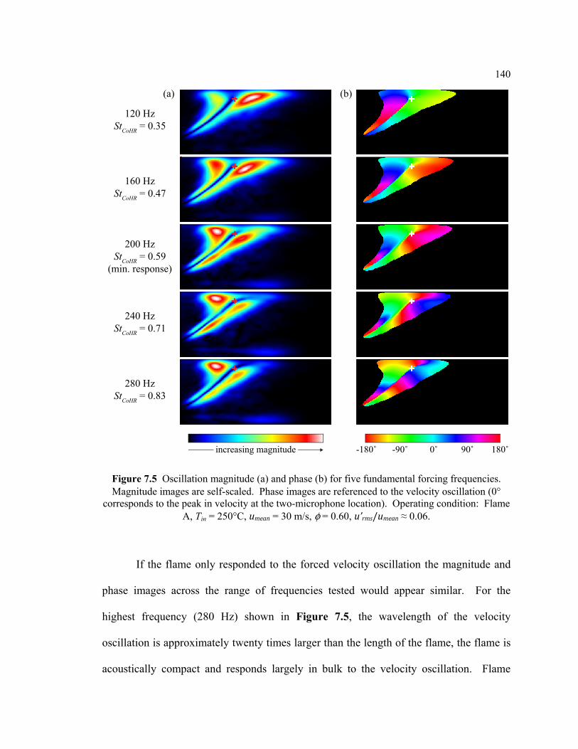
Global flame response to forced velocity oscillations between 100 and 440 Hz
was measured over a wide range of operating conditions. Nearly all measurements
showed similar qualitative behavior; gain decreased with increasing frequency until
reaching a minimum value at a frequency fmin. After reaching a local minimum, gain
increased with frequency. The frequency of minimum response fmin varied with operating
condition and was found to be related to the mean velocity in the injector umean and a
characteristic flame length determined from stable flame imaging. In addition, the phase
between velocity oscillations and heat release rate oscillations scaled with mean velocity
and flame length.
The global response of the flame was separated into acoustic and convective
components by modeling the response of the flame to a purely acoustic wavelength
velocity oscillation. The phase of the reconstructed convective response was
characteristic of a response to a flow disturbance originating from the end of the injector
centerbody, the anchoring point of the flame. Phase-synchronized imaging of select
flames over a range of frequencies showed global flame response was controlled by the
interaction between axial velocity oscillations and vortical disturbances shed from the
injector centerbody throughout the flame brush.
v
Table of Contents
List of Figures .............................................................................................................. viii
List of Tables ............................................................................................................... xiv
Nomenclature ............................................................................................................... xv
Acknowledgements ...................................................................................................... xviii
2.3 Pressure, Velocity, and Global Chemiluminescence Signal Analysis ............ 43 2.3.1 Linear Spectrum and Single-sided Power Spectral Density ................. 43 2.3.2 Forced and Self-excited Flame Signal Analysis Comparison .............. 44 2.3.3 Two-microphone Method for Calculating Velocity Oscillations ......... 47 2.3.4 Coherence and Single-sided Cross Spectral Density (SSCSD) ............ 51 2.3.5 Uncertainty in the Slope of a Linear Fit ............................................... 52
2.4 Flame Image Processing ................................................................................. 53 2.4.1 Forward and Inverse Abel Transforms ................................................. 53
3.1 Effect of Combustor Length (LC) on Stability ................................................ 63 3.1.1 Oscillation Mode Shape ....................................................................... 65 3.1.2 Pressure and Frequency of Self-excited Instabilities ............................ 68
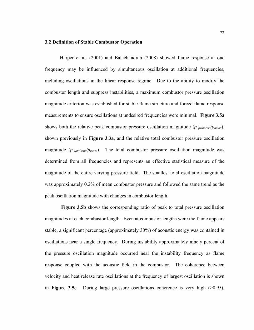
3.2 Definition of Stable Combustor Operation ..................................................... 72
Chapter 6 Global Flame Response ............................................................................... 95
6.1 Operating Conditions ...................................................................................... 96 6.2 Example Flame Transfer Function ................................................................. 97 6.3 All Flame Transfer Functions ......................................................................... 100
6.3.1 Strouhal number (StCoHR) Scaling ......................................................... 101 6.3.2 Frequency of Minimum Gain Response ............................................... 109
6.4 Separation of Acoustic and Convective Flame Response Components ......... 119 6.4.1 Acoustic Flame Response Component Model ..................................... 119 6.4.2 Total, Acoustic, and Convective Flame Phase Response ..................... 121
Chapter 7 Local Flame Response ................................................................................ 131
7.1 Operating Conditions, Global Flame Response, and Structure Comparison .. 131 7.2 Spatially-resolved Flame Dynamics ............................................................... 136
7.2.1 Stable and Time-averaged Flame Structure Comparison ..................... 136
vii
7.2.2 Magnitude and Phase of Local Heat Release Rate Oscillation ............ 138 7.2.3 Spatially-resolved Heat Release Rate Distribution and Fluctuation .... 142
Figure 1.1 New (left) and damaged (right) gas turbine combustor burner assembly (from Huang and Yang, 2009, originally from Goy et al., 2005.) ........ 2
Figure 1.2 Combustion instability process description (modified from Zinn and Lieuwen, 2005). .................................................................................................... 5
Figure 1.3 Heat release rate response to velocity perturbations path (Lieuwen and Cho, 2005). ..................................................................................................... 9
Figure 1.4 Linear and nonlinear flame response regimes. ......................................... 11
Figure 1.5 Conical, V-flame, and M-flame configurations. The flame front is represented by the red dashed lines. Arrows indicate flow direction. ................. 14
Figure 2.1 Schematic of research combustor. Flow is from left to right. ................. 31
Figure 2.2 Schematic of injector geometry and pressure transducer locations. ......... 33
Figure 2.3 Schematic of fused quartz and variable-length combustors. .................... 35
Figure 2.4 Siren and valves used to control forced velocity oscillation. ................... 37
Figure 2.5 Examples of stable (a) and time-averaged (b) flame projection images (operating condition: Tin = 250°C, umean = 40 m/s, φ = 0.65). The faint hexagons present in both images result from the fiber optic bundles in the camera that connect the intensifier to the CCD. Both images are self-scaled. Radial and axial distances are in centimeters. ...................................................... 40
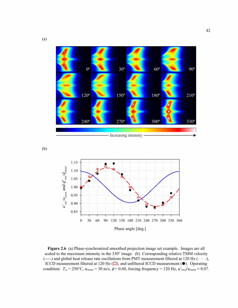
Figure 2.6 (a) Phase-synchronized smoothed projection image set example. Images are all scaled to the maximum intensity in the 330° image. (b) Corresponding relative TMM velocity (–––) and global heat release rate oscillations from PMT measurement filtered at 120 Hz (– – –), ICCD measurement filtered at 120 Hz (), and unfiltered ICCD measurement (). Operating condition: Tin = 250°C, umean = 30 m/s, φ = 0.60, forcing frequency = 120 Hz, u’rms/umean ≈ 0.07. ............................................................... 42
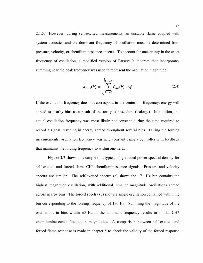
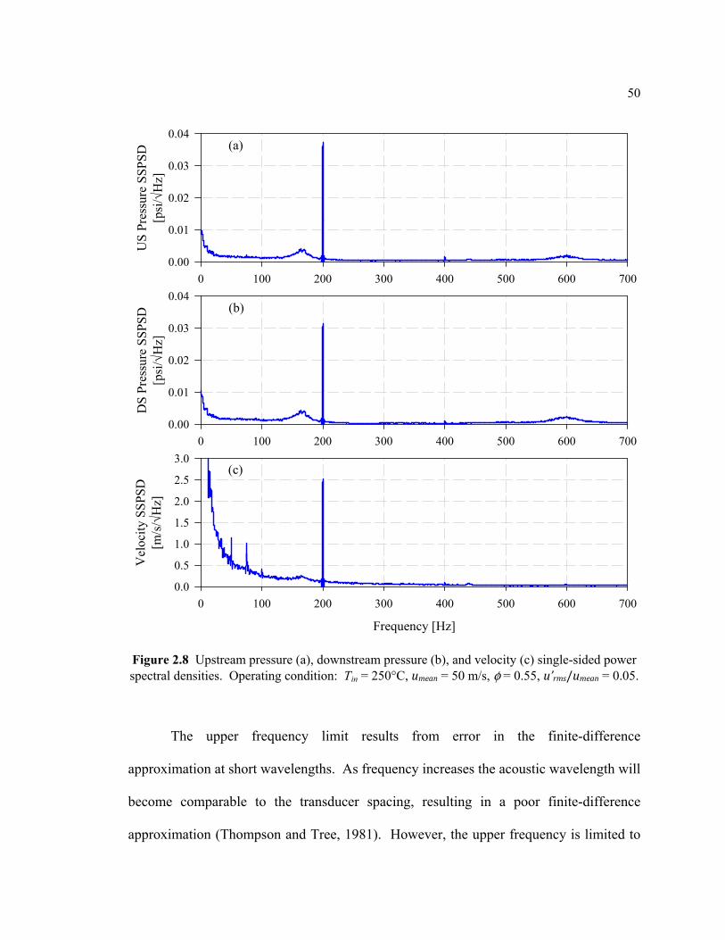
Figure 2.7 CH* single-sided power spectral densities for forced (a & b) and self-excited (c & d) flames. Operating condition: Tin = 250°C, umean = 40 m/s, φ = 0.65, u’rms/umean = 0.10 (forced), LC = 18 in. (self-excited). ............................. 46
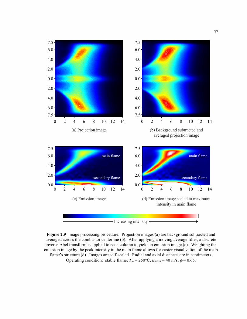
Figure 2.9 Image processing procedure. Projection images (a) are background subtracted and averaged across the combustor centerline (b). After applying a moving average filter, a discrete inverse Abel transform is applied to each column to yield an emission image (c). Weighting the emission image by the peak intensity in the main flame allows for easier visualization of the main flame’s structure (d). Images are self-scaled. Radial and axial distances are in centimeters. Operating condition: stable flame, Tin = 250°C, umean = 40 m/s, φ = 0.65. ........................................................................................................ 57
Figure 2.10 Mean flame sheet location (black line) in the main and secondary flames. The image is scaled to the maximum intensity in the main flame. Radial and axial distances are in centimeters. Operating condition: stable flame, Tin = 250°C, umean = 40 m/s, φ = 0.65. ....................................................... 59
Figure 2.11 Examples of emission (a) and revolved (b) flame images. Images are self-scaled. Radial and axial distances are in centimeters. Operating condition: stable flame, Tin = 250°C, umean = 40 m/s, φ = 0.65. .......................... 60
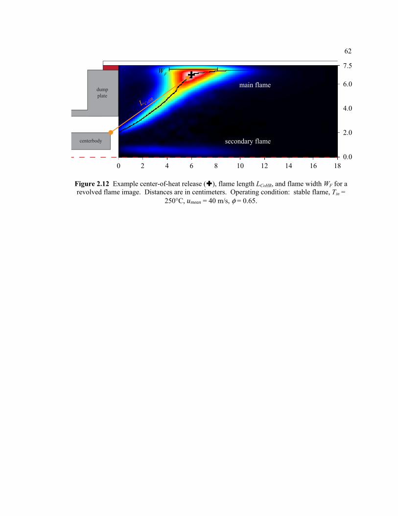
Figure 2.12 Example center-of-heat release (), flame length LCoHR, and flame width WF for a revolved flame image. Distances are in centimeters. Operating condition: stable flame, Tin = 250°C, umean = 40 m/s, φ = 0.65. ......... 62
Figure 3.1 Combustor pressure single-sided power spectral densities for combustor lengths between 18 in. and 59 in. Operating condition: Tin = 250°C, umean = 40 m/s, φ = 0.65. .......................................................................... 65
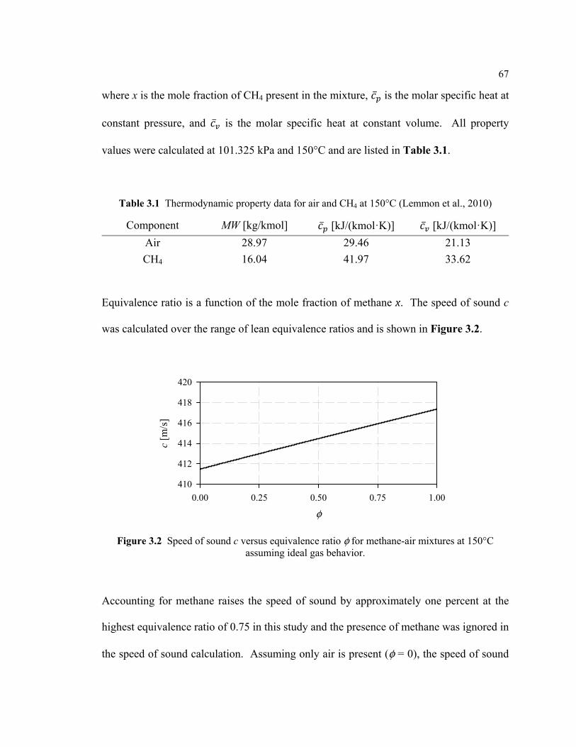
Figure 3.2 Speed of sound c versus equivalence ratio φ for methane-air mixtures at 150°C assuming ideal gas behavior. ................................................................. 67
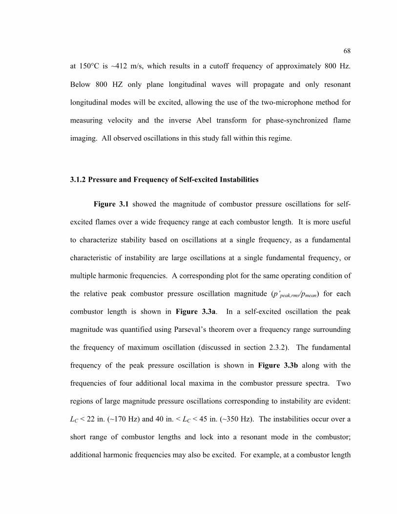
Figure 3.3 (a) Relative peak combustor pressure oscillation magnitude, (b) corresponding frequency of oscillation () and additional frequencies of local maxima in combustor pressure () versus LC. Operating condition: Tin = 250°C, umean = 40 m/s, φ = 0.65. .......................................................................... 70
Figure 3.4 Relative peak combustor pressure oscillation magnitude versus the phase difference between pressure and heat release rate oscillations. Operating condition: Tin = 250°C, umean = 40 m/s, φ = 0.65. ............................... 71
Figure 3.5 Relative peak and total combustor pressure oscillation magnitudes (a), the ratio between peak and total pressure oscillation magnitudes (b), and coherence between velocity and heat release rate (c) versus LC. Operating condition: Tin = 250°C, umean = 40 m/s, φ = 0.65. ................................................ 74
x
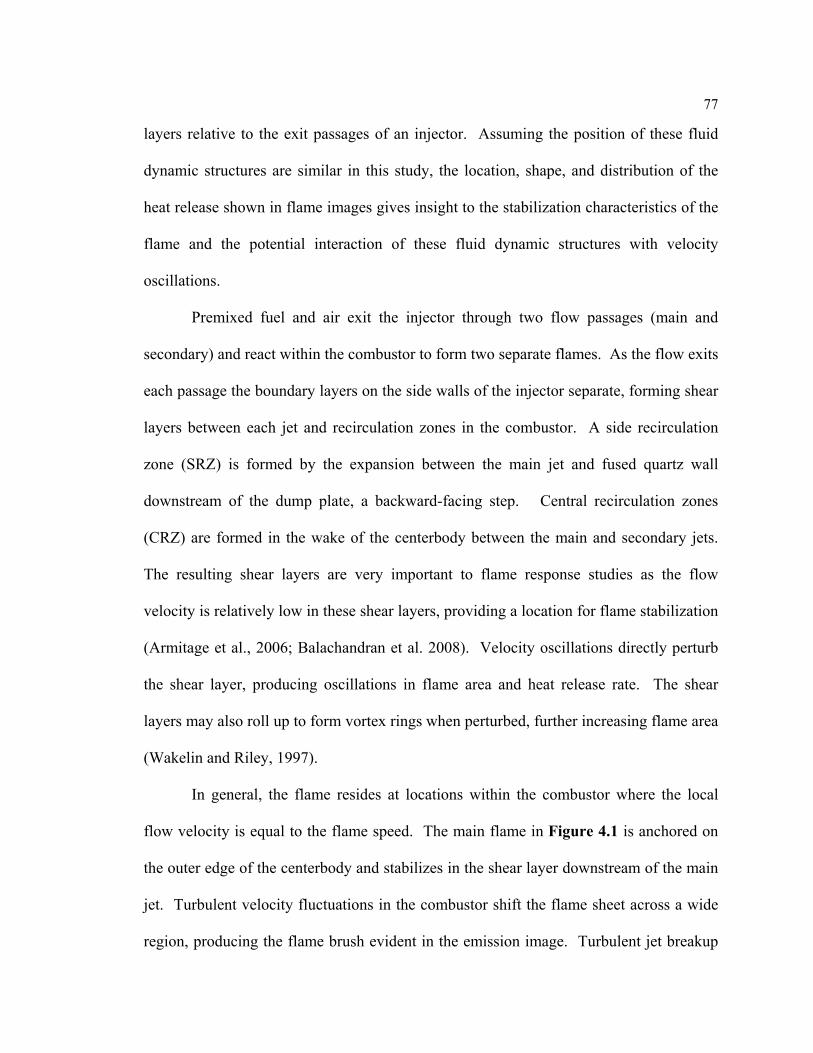
Figure 4.1 (a) Stable flame emission image with mean flame sheet location (black lines) for both main and secondary flames. Image is scaled to peak intensity in the main flame. Operating condition: Tin = 250°C, umean = 40 m/s, φ = 0.65. (b) Corresponding schematic of side recirculation zone (SRZ), central recirculation zones (CRZ), and jet locations. Radial and axial distances are in centimeters. ................................................................................. 78
Figure 4.2 Center-of-heat release locations in context of the combustor of both emission and revolved flame images for eighty-eight operating conditions. ....... 80
Figure 4.3 Percent difference between predicted LCoHR and measured LCoHR of revolved images. ................................................................................................... 83
Figure 4.4 Stable flame width (WF) versus flame length (LCoHR) with line-of-best fit. .......................................................................................................................... 84
Figure 5.1 Relative flame response magnitude (a) and phase (b) between velocity and heat release rate for self-excited and forced flames. Operating condition: Tin = 250°C, umean = 40 m/s, φ = 0.65. Forced 1, Forced 2, Forced 3, Self-excited ........................................................................................................ 86
Figure 5.2 Frequency of heat release rate, pressure, and velocity oscillations (a) and coherence between velocity and heat release rate (b). Operating condition: Tin = 250°C, umean = 40 m/s, φ = 0.65. Forced 1, Forced 2, Forced 3, Self-excited ....................................................................................... 88
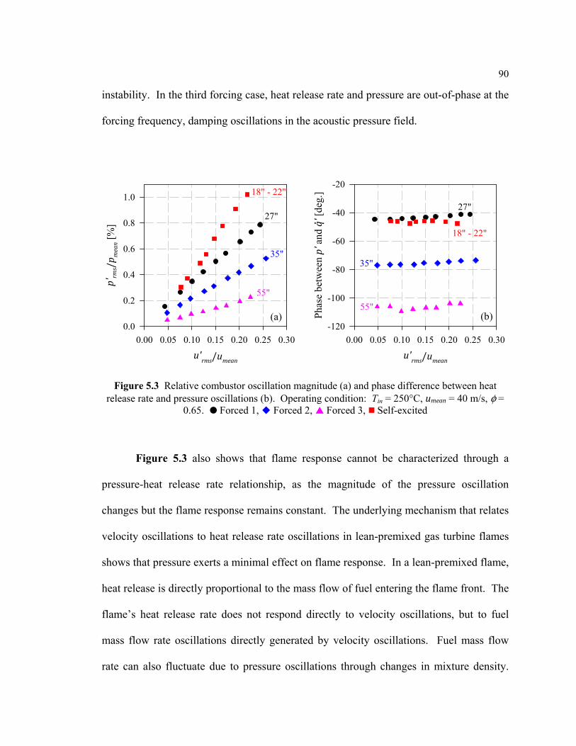
Figure 5.3 Relative combustor oscillation magnitude (a) and phase difference between heat release rate and pressure oscillations (b). Operating condition: Tin = 250°C, umean = 40 m/s, φ = 0.65. Forced 1, Forced 2, Forced 3, Self-excited ........................................................................................................ 90
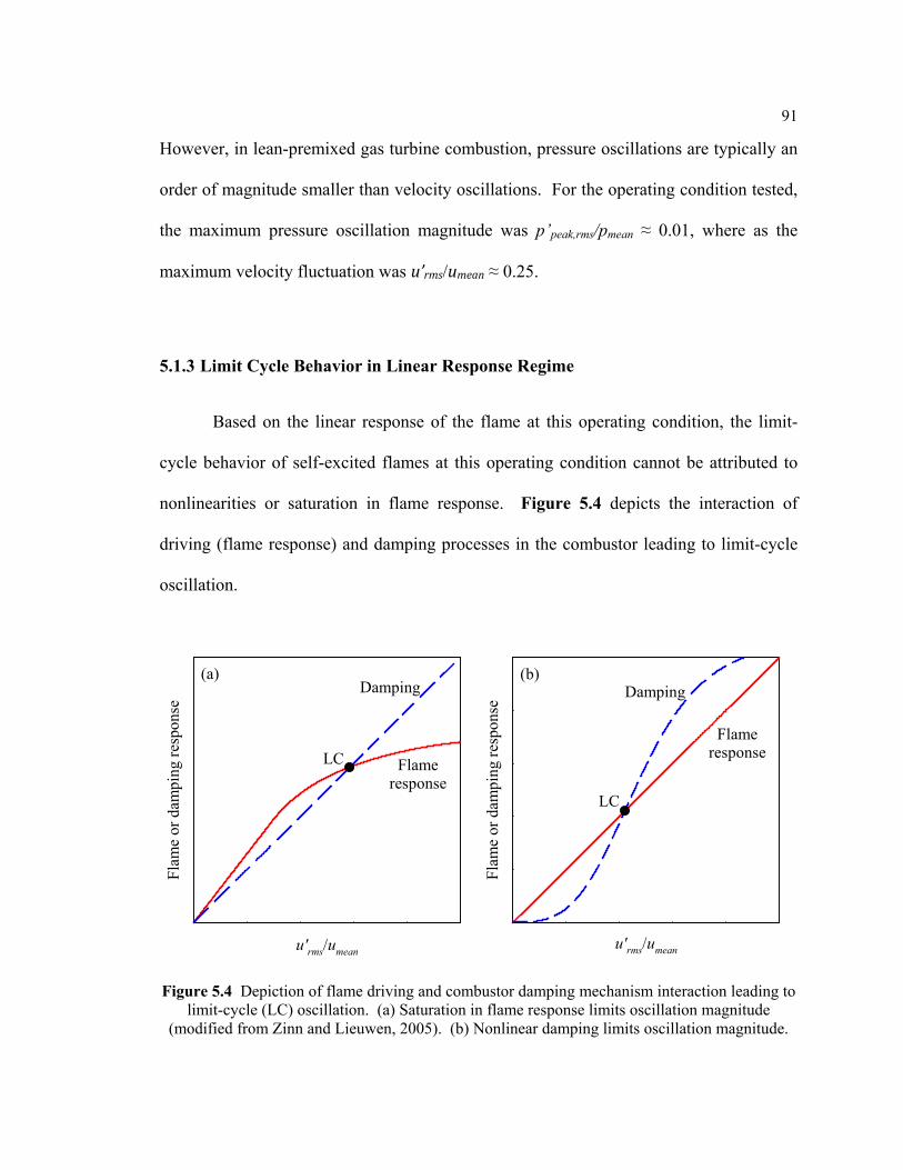
Figure 5.4 Depiction of flame driving and combustor damping mechanism interaction leading to limit-cycle (LC) oscillation. (a) Saturation in flame response limits oscillation magnitude (modified from Zinn and Lieuwen, 2005). (b) Nonlinear damping limits oscillation magnitude. ............................... 91
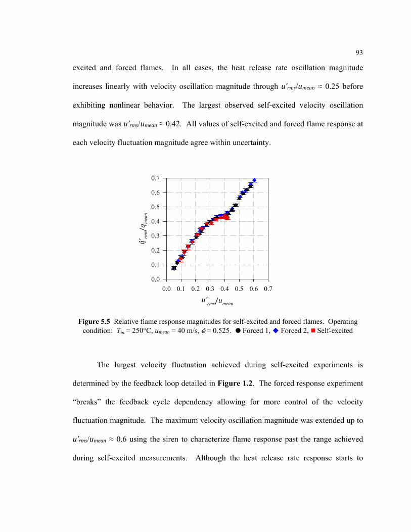
Figure 5.5 Relative flame response magnitudes for self-excited and forced flames. Operating condition: Tin = 250°C, umean = 40 m/s, φ = 0.525. Forced 1, Forced 2, Self-excited ................................................................... 93
Figure 6.1 Example flame transfer function gain (a) and phase (c) for a single operating condition. The coefficient of variation between measurements at each forcing frequency are included for both gain (b) and phase (d). Operating condition: Tin = 250°C, umean = 30 m/s, φ = 0.65, u’rms/umean ≈ 0.05. ...................................................................................................................... 105
xi
Figure 6.2 Flame transfer function gain (a) and phase (c) versus forcing frequency for a thirty-eight unique operating conditions. The coefficient of variation between flame transfer functions (CVFF) and the variation in a single flame transfer function (CV1) are included for both gain (b) and phase (d). ......................................................................................................................... 106
Figure 6.3 Flame transfer function gain (a) and phase (c) versus StCoHR for a thirty-eight unique operating conditions. The coefficient of variation between flame transfer functions (CVFF) and the variation in a single flame transfer function (CV1) at each forcing frequency are shown for both gain (b) and phase (d). The coefficient of variation between flame transfer functions after plotting versus StCoHR (CVSt) is indicated by the black dashed line. ............ 107
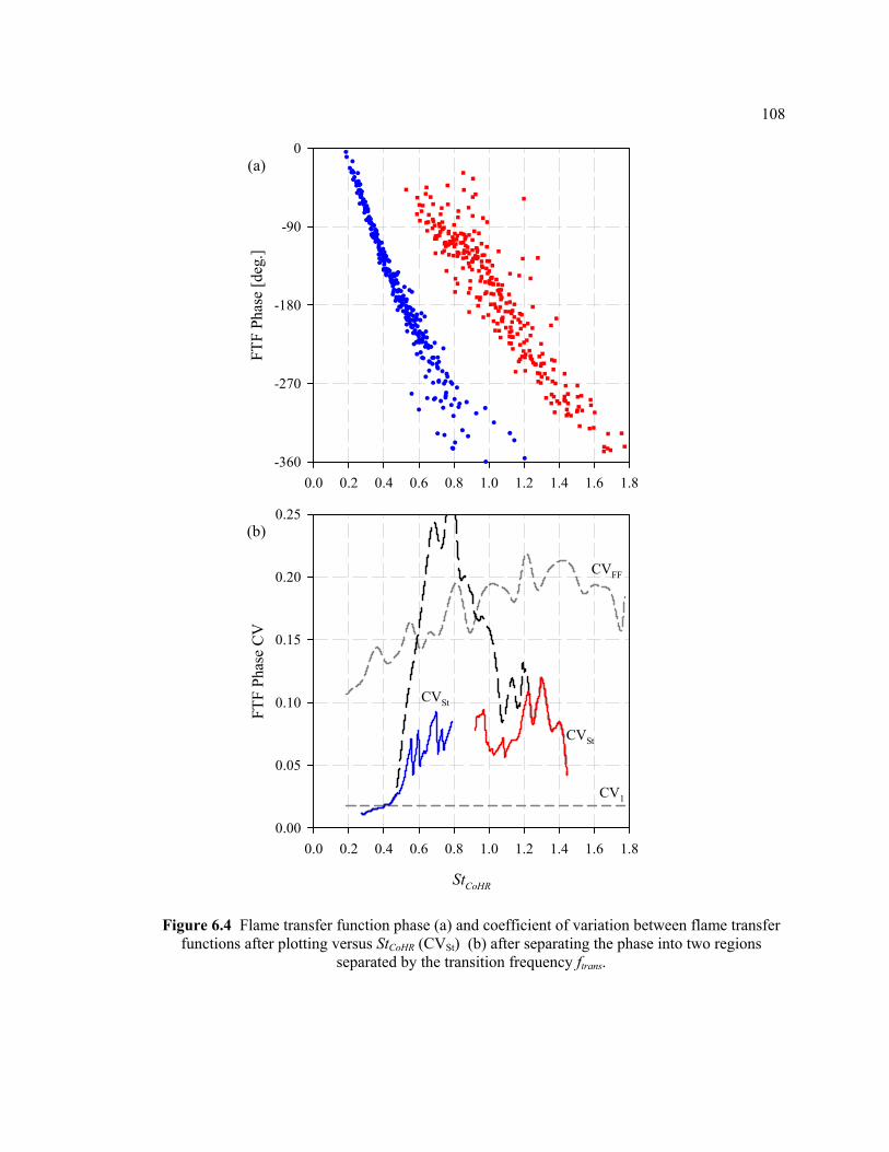
Figure 6.4 Flame transfer function phase (a) and coefficient of variation between flame transfer functions after plotting versus StCoHR (CVSt) (b) after separating the phase into two regions separated by the transition frequency ftrans. ....................................................................................................................... 108
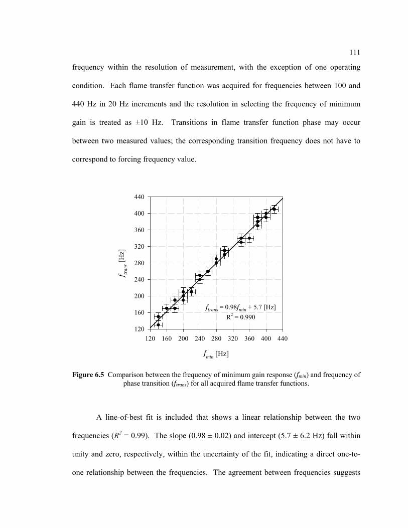
Figure 6.5 Comparison between the frequency of minimum gain response (fmin) and frequency of phase transition (ftrans) for all acquired flame transfer functions. .............................................................................................................. 111
Figure 6.6 Frequency of minimum flame response versus mean axial velocity. Thirty-six minimum responses were observed but several data points overlap. .. 113
Figure 6.7 Strouhal number values at frequency of minimum response versus flame length. Lines are predicted values of Strouhal number based on a vortical disturbance from the centerbody end (CB), interaction between swirl number oscillations and a vortical disturbance from the centerbody end (SW-CB), and interaction between axial velocity oscillations and vortical disturbance from the centerbody end (u’-CB). ..................................................... 118
Figure 6.8 Example of the phase difference between velocity and heat release rate oscillations for measured (FTF), modeled acoustic, and reconstructed convective oscillations between 100 and 440 Hz. Operating condition: Tin = 250°C, umean = 30 m/s, φ = 0.60, u’rms/umean ≈ 0.05. ............................................ 122
Figure 6.9 All phase differences between velocity and heat release oscillations for measured (FTF), modeled acoustic, and reconstructed convective oscillations versus (a) frequency and (b) StCoHR. ................................................... 124
Figure 6.10 Phase differences with lines-of-best fit for the measured, modeled acoustic, and reconstructed convective components of flame response at low StCoHR. .................................................................................................................... 125
xii
Figure 6.11 Convective component of flame response with calculated phase delays for convective perturbations from the centerbody end (CB) and swirler vane exit (SW). ..................................................................................................... 129
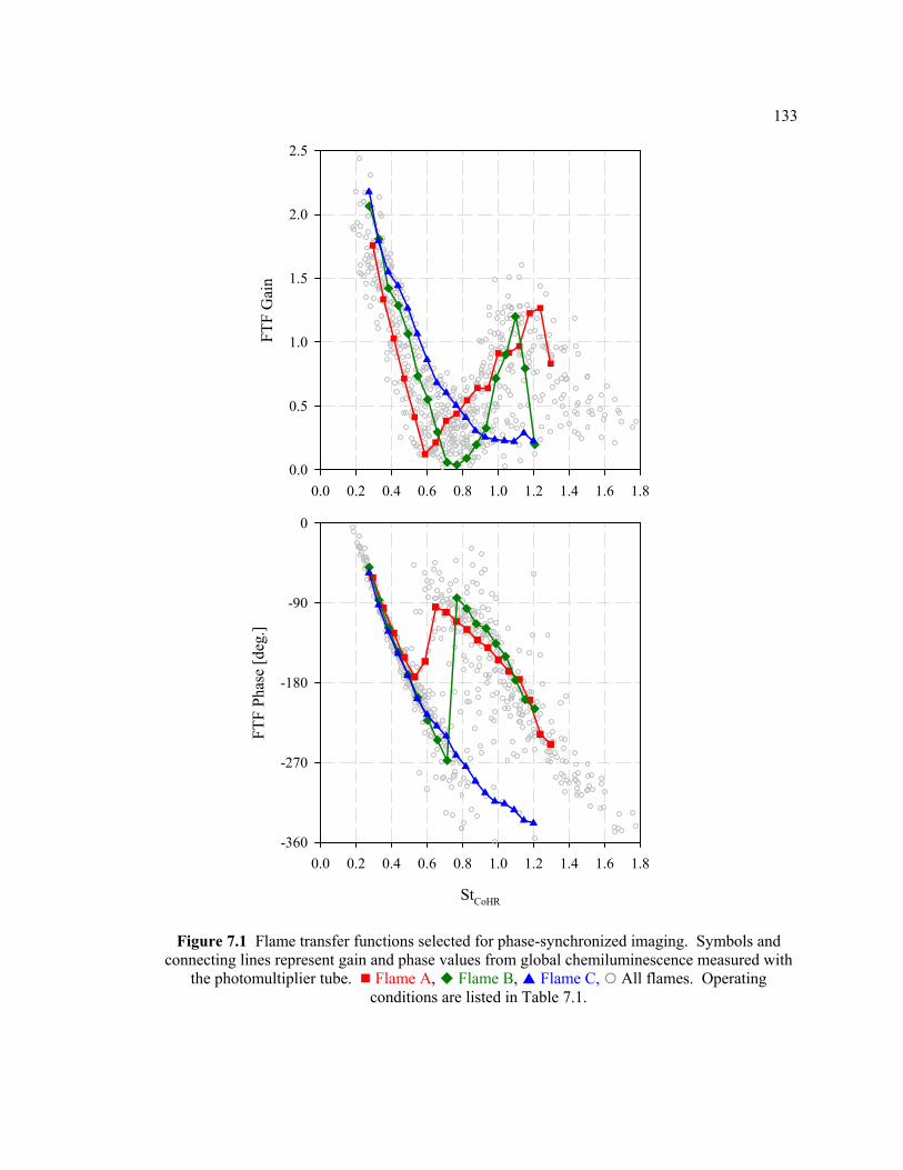
Figure 7.1 Flame transfer functions selected for phase-synchronized imaging. Symbols and connecting lines represent gain and phase values from global chemiluminescence measured with the photomultiplier tube. Flame A, Flame B, Flame C, All flames. Operating conditions are listed in Table 7.1. ........................................................................................................................ 133
Figure 7.2 StCoHR values of all phase-synchronized image sets. Symbols represent gain and phase determined from global chemiluminescence acquired measured with the ICCD camera. Lines represent gain and phase determined from chemiluminescence measured with the photomultiplier tube. Flame A, Flame B, Flame C, All flames. Operating conditions are listed in Table 7.1. ................................................................................................ 134
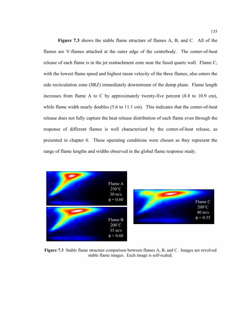
Figure 7.3 Stable flame structure comparison between flames A, B, and C. Images are revolved stable flame images. Each image is self-scaled. ................. 135
Figure 7.4 Stable and time-averaged images (a) and corresponding flame length LCoHR and width WF (b). Operating condition: Flame A, Tin = 250°C, umean = 30 m/s, φ = 0.60, u’rms/umean ≈ 0.06. .................................................................... 137
Figure 7.5 Oscillation magnitude (a) and phase (b) for five fundamental forcing frequencies. Magnitude images are self-scaled. Phase images are referenced to the velocity oscillation (0° corresponds to the peak in velocity at the two-microphone location). Operating condition: Flame A, Tin = 250°C, umean = 30 m/s, φ = 0.60, u’rms/umean ≈ 0.06. .................................................................... 140
Figure 7.6 Phase-synchronized flame (a) and fluctuation (b) images of Flame A at a frequency of 120 Hz. Operating condition: Tin = 250°C, umean = 30 m/s, φ = 0.60, u’rms/umean ≈ 0.06. ................................................................................. 143
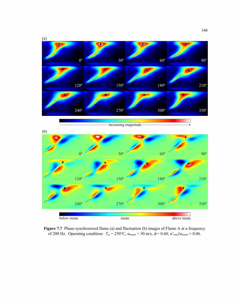
Figure 7.7 Phase-synchronized flame (a) and fluctuation (b) images of Flame A at a frequency of 200 Hz. Operating condition: Tin = 250°C, umean = 30 m/s, φ = 0.60, u’rms/umean ≈ 0.06. ................................................................................. 146
Figure 7.8 Oscillation magnitude (a) and phase (b) for six fundamental forcing frequencies. Magnitude images are self-scaled. Phase images are referenced to the velocity oscillation (0° corresponds to the peak in velocity at the TMM location). Operating condition: Flame B, Tin = 200°C, umean = 35 m/s, φ = 0.60, u’rms/umean ≈ 0.06. ........................................................................................ 149
xiii
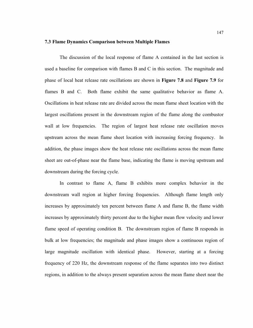
Figure 7.9 Oscillation magnitude (a) and phase (b) for five fundamental forcing frequencies. Magnitude images are self-scaled. Phase images are referenced to the velocity oscillation (0° corresponds to the peak in velocity at the TMM location). Operating condition: Flame C, Tin = 200°C, umean = 40 m/s, φ = 0.55, u’rms/umean ≈ 0.06. ........................................................................................ 150
xiv
List of Tables
Table 1.1 Analytical (A), computational (C), and experimental (E) studies investigating the interaction of multiple response mechanisms in premixed flames. ................................................................................................................... 27
Table 3.1 Thermodynamic property data for air and CH4 at 150°C (Lemmon et al., 2010) ............................................................................................................... 67
Table 6.1 Independent parameters varied and ranges for flame response measurements. ...................................................................................................... 96
Table 6.2 Linear fit properties of flame transfer function phase and convective component phase. Operating condition: Tin = 250°C, umean = 30 m/s, φ = 0.60, u’rms/umean = 0.05. ........................................................................................ 123
Table 6.3 Linear fit properties of flame transfer function phase and convective component phase. ................................................................................................. 126
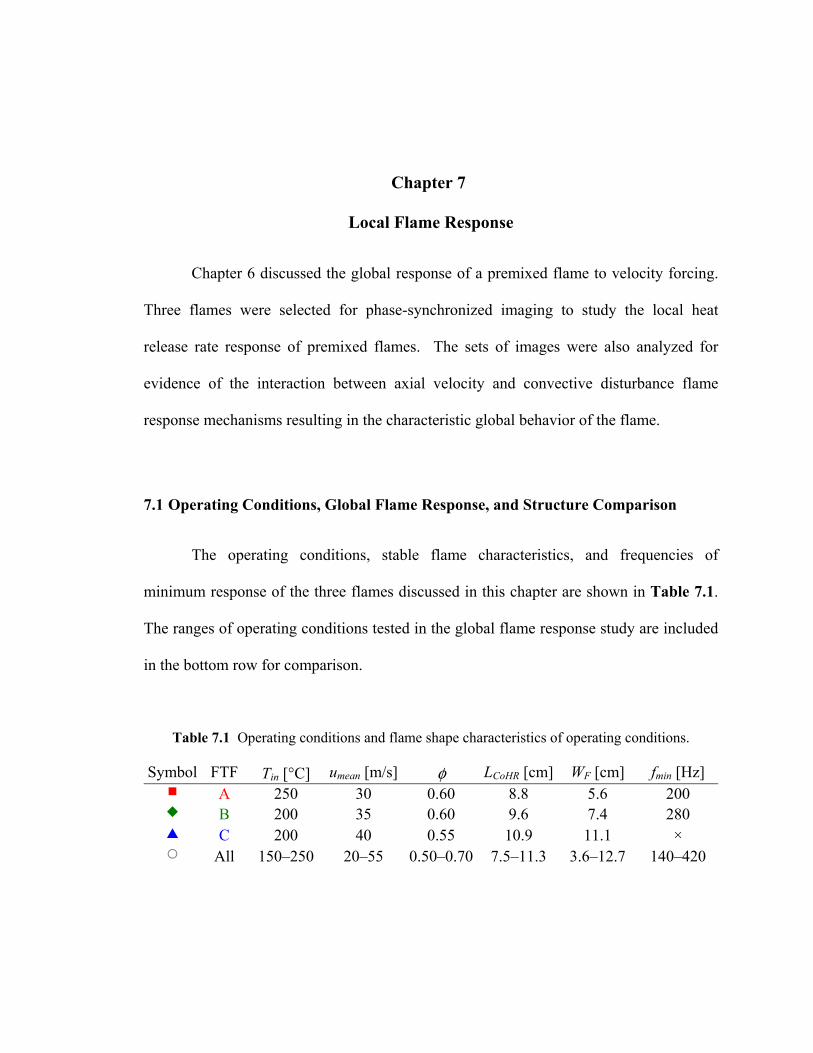
Table 7.1 Operating conditions and flame shape characteristics of operating conditions. ............................................................................................................. 131
xv
Nomenclature
A Area, or Amplitude of oscillation
a.i.u. Arbitrary intensity unit
c Speed of sound, m/s
f Frequency, Hz
fs Sampling frequency, samples/s
FTF Flame transfer function
G Single-sided power spectral density or FTF gain
i, k Index variables
I Projection image
j Imaginary unit √−1
J Bessel function
L Length
MW Molecular weight, kg/kmol
N Number of samples
p Pressure
Heat release
Coefficient of determination
Ru Universal gas constant
S Flame speed
St Strouhal number
t Time
xvi
T Temperature, °C or Period, s
TMM Two-microphone method
u Velocity, m/s
V Volume
W Width
x, r, y, z Spatial coordinate
Greek Symbols
α Flame angle
Ratio of specific heats
ε Emission image
Δ Difference
φ Equivalence ratio
λ Wavelength
θa,b Phase of quantity a relative to quantity b
ρ Density, kg/m3
σ(a) Absolute uncertainty of quantity a
ω Angular frequency, rad/s
∇ Gradient
xvii
Subscripts
acs Acoustic quantity
CoHR Center-of-heat release
C Combustor
conv Convective quantity
ds Downstream
f, F Flame
fund Fundamental frequency
in Injector inlet
L Laminar
mean Arithmetic mean
min Minimum value
mix Mixture
rms Root-mean-square
trans Transition
us Upstream
Superscripts
′ Fluctuation
* Excited species
→ Vector field
· Rate
xviii
Acknowledgements
I thank my advisor, Dr. Domenic Santavicca, for his patience, valuable guidance,
and encouragement during my graduate study. I would also like to thank Dr. Santoro, Dr.
Turns, Dr. van Duin, and Dr. Vander Wal for serving on my doctoral committee and their
guidance and assistance.
I also express my gratitude to Dr. Bryan Quay for designing the combustor
facility, sharing his extensive knowledge of instrumentation and measurement
techniques, and his guidance on setting up and running the experiment used in this study.
I thank Dr. Jong Guen Lee and Dr. Kyutae Kim both for the helpful discussions related to
this research. I would also like to thank Larry Horner for fabricating most of the facility
used in this study and his advice on modifications and Sally Mills, Virginia Smith, and
John Raiser for all of their help and assistance.
I also thank my fellow students in the Turbulent Combustion Lab, Nick Bunce,
Simone D’Emidio, Alex de Rosa, Brian Jones, Hyung Ju Lee, Bridget O’Meara, Poravee
Orawannukul, Janith Samarasingh, and Mike Szedlmayer for their friendship, support,
and assistance and I am thankful for the time spent with them over the last six years.
The research reported in this dissertation was sponsored by Solar Turbines, Inc. I
especially thank Jim Blust and Ramu Bandaru for their support of this project.
Finally, I thank my parents, my sister Amanda, and my brother Thomas for their
love and support.
Chapter 1
Introduction
1.1 Gas Turbine and Combustion Instability Background
Gas turbines operating on natural gas are a major component of the electrical
energy production system in the United States, producing approximately twenty-five
percent of all electrical energy in 2011 (US DOE/EIA, 2012). Industrial gas turbines
occupy a unique role in electrical production; they are used primarily in mid-merit or
peaking power plants due to the ability to start (zero to full load) on the order of minutes
and adjust power output on the order of seconds to match demand (Walsh and Fletcher,
2004). Almost all other power production methods provide base load power production
due to limited time response ability. Even with an increased focus on nuclear and
renewable energy in the United States over the next few decades, gas turbines will remain
a vital component of electrical energy production (US DOE/EIA, 2011).
Early conventional gas turbines used diffusion flame combustors resulting in
reliable performance and high stability. Unfortunately, diffusion flames generate high
reaction zone temperatures that result in elevated oxides of nitrogen (NOx) production.
Starting in the mid-1980s, emission limits led to the development of dry low NOx lean-
premixed gas turbines (LPGT). Fuel and air are mixed before the flame zone in lean-
premixed combustion, eliminating stoichiometric regions that result in elevated flame
temperature. The overall reaction zone temperature is reduced, limiting thermal NO
2
production. Prior to the development of lean-premixed gas turbines, water or steam was
injected into the combustor to lower the temperature in the reaction zone; “dry” indicates
additional water is not required. Current low NOx systems without additional exhaust gas
treatment are capable of achieving less than 9 ppmv NOx in the exhaust at 15% excess
oxygen (Baird et al., 2010). This represents a significant improvement over conventional
combustors which produced several hundred ppmv NOx (US EPA, 1993).
Unfortunately, lean-premixed combustion systems are vulnerable to combustion
instabilities. Combustion instabilities are relatively high amplitude oscillations sustained
by coupling between flame heat release and system acoustics. They are self-excited
oscillations, involving complex interaction between the acoustic pressure field, particle
velocity field, local flame heat release, and system boundaries. Large instabilities can
cause flame flashback, blow-off, and increase vibration resulting in structural damage to
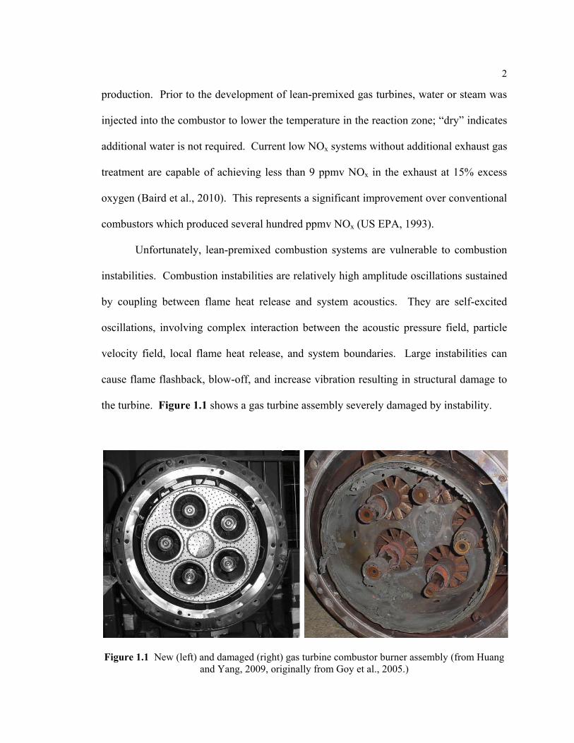
the turbine. Figure 1.1 shows a gas turbine assembly severely damaged by instability.
Figure 1.1 New (left) and damaged (right) gas turbine combustor burner assembly (from Huang and Yang, 2009, originally from Goy et al., 2005.)
3
Pressure fluctuations damaged welds on the fuel lines in one of the five injectors,
altering the fuel injection path into the combustor and flame location. The resultant
change in flame position melted the diffusion plate on the burner assembly face.
Many combustion systems, including both diffusion and lean-premixed gas
turbine configurations, are potentially sensitive to combustion instabilities for two
primary reasons: (i) the energy required to drive pressure oscillations is typically a small
fraction of the energy released by chemical reaction, and (ii) most combustion systems
are nearly fully closed chambers with limited damping (Huang and Yang, 2009). Lean-
premixed gas turbine systems are particularly sensitive to combustion instabilities for
additional reasons. The equivalence ratio of the flame is typically close to the lean
blowout limit to reduce flame temperature. During unstable combustion, the equivalence
ratio of the reactants can fluctuate due to coupling between the fuel delivery system and
pressure oscillations in the combustor. If the equivalence ratio drops below the lean
blowout limit, the flame will extinguish. Once the equivalence ratio increases above the
lean blowout limit the flame can reignite, generating large variations in heat release
(Lieuwen and McManus, 2003). Flames in lean-premixed gas turbines are typically short
compared to longitudinal acoustic wavelengths and can be considered acoustically
compact, allowing for easy coupling between heat release and system acoustics (Huang
and Yang, 2009). Conventional diffusion flame combustors are typically supplied
secondary dilution or film cooling air through the liner to reduce the temperature of
combustion products and protect the liner wall. These liners contain many small
apertures that act as acoustic attenuators, potentially dampening resonant pressure
4
fluctuations in the combustor. Current premixed combustors use limited secondary air,
reducing the dampening effects present in older conventional systems (Keller, 1995).
This study focuses directly on one process associated with combustion
instabilities: the heat release rate response of a flame to velocity oscillations, also
referred to as flame response to velocity oscillation. The following sections describe the
overall combustion instability process and the specific role of flame response within the
overall process is discussed.
1.2 Combustion Instability Cycle
Typical combustion instabilities occur at or near frequencies related to the
resonant acoustic modes of the overall combustion system. Lower frequency instabilities
occur at bulk (Helmholtz-resonator type) or longitudinal modes and are usually on the
order of several hundred hertz in gas turbine systems. Higher frequency instabilities
occur at transverse (radial, azimuthal, or tangential) modes and are typically on the order
of several thousand hertz (Zinn and Lieuwen, 2005). Instabilities associated with
longitudinal modes are examined in this study.
1.2.1 Instability Feedback Cycle
The feedback cycle necessary to sustain an instability in a premixed combustor is
shown in Figure 1.2. The overall cycle is divided into three processes: (1) heat release
rate oscillations couple with pressure oscillations, (2) pressure oscillations couple with
5
velocity oscillations, and (3) velocity oscillations couple with heat release rate
oscillations, completing the cycle.
Figure 1.2 Combustion instability process description (modified from Zinn and Lieuwen, 2005).
Positive coupling between properties in all three processes is necessary to
maintain unstable combustion. Each process is described in more detail in the following
three sections. The feedback process is inherently cyclical; the numbering used is only
for identification purposes. Coupling between heat release rate and pressure was
identified first by Lord Rayleigh (1878) as critical to the feedback process and is
described in the following section.
1.2.1.1 Process 1 – Heat Release Rate/Pressure Coupling (Rayleigh’s Criterion)
In order for unstable combustion to be maintained, a perturbation in heat release
rate must positively couple with the acoustic pressure field in the combustor. Lord
Rayleigh first proposed the correct conditions for coupling during the mid-1870s,
proposing that
Heat release rate oscillations q'
Pressure oscillations p'
Velocity oscillations u'
13
2
∙
6
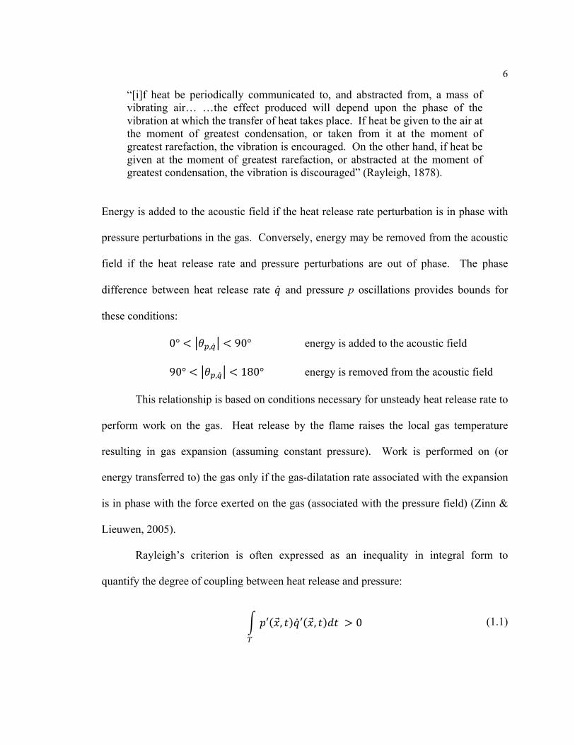
“[i]f heat be periodically communicated to, and abstracted from, a mass of vibrating air… …the effect produced will depend upon the phase of the vibration at which the transfer of heat takes place. If heat be given to the air at the moment of greatest condensation, or taken from it at the moment of greatest rarefaction, the vibration is encouraged. On the other hand, if heat be given at the moment of greatest rarefaction, or abstracted at the moment of greatest condensation, the vibration is discouraged” (Rayleigh, 1878).
Energy is added to the acoustic field if the heat release rate perturbation is in phase with
pressure perturbations in the gas. Conversely, energy may be removed from the acoustic
field if the heat release rate and pressure perturbations are out of phase. The phase
difference between heat release rate and pressure p oscillations provides bounds for
these conditions:
0° < , < 90° energy is added to the acoustic field
90° < , < 180° energy is removed from the acoustic field
This relationship is based on conditions necessary for unsteady heat release rate to
perform work on the gas. Heat release by the flame raises the local gas temperature
resulting in gas expansion (assuming constant pressure). Work is performed on (or
energy transferred to) the gas only if the gas-dilatation rate associated with the expansion
is in phase with the force exerted on the gas (associated with the pressure field) (Zinn &
Lieuwen, 2005).
Rayleigh’s criterion is often expressed as an inequality in integral form to
quantify the degree of coupling between heat release and pressure:
′( , ) ′( , ) > 0 (1.1)
7
If the two perturbations are in phase, Rayleigh’s criterion is satisfied and the above
integral is positive. If the perturbations are out of phase, heat release rate perturbations
will damp pressure perturbations and the integral is negative.
1.2.1.2 Process 2 – Pressure/Velocity Coupling
Satisfaction of Rayleigh’s criterion is necessary for sustaining unstable
combustion, but not sufficient. Pressure perturbations generated by heat release rate
perturbations must couple with other fluid properties in the combustor to sustain the
feedback cycle. The fluid properties of most importance in the feedback cycle are
particle velocity (or simply velocity) and equivalence ratio as they directly relate to the
fuel flow rate into the flame. In perfectly premixed systems, pressure perturbations only
generate velocity perturbations, modulating the mixture mass flow rate.
However, land-based gas turbines operate in partially premixed (also called
technically premixed) mode where fuel is injected a short distance upstream of the flame
and may not fully and uniformly mix with inlet air before reaching the flame. In these
systems, pressure perturbations can generate both velocity and equivalence ratio
perturbations. The relationship between pressure, particle velocity, and equivalence ratio
perturbations depends on several factors, including combustor geometry and boundary
conditions, fuel injection location and method, and the characteristic impedance of the
medium.
8
This study focuses on the heat release response of fully premixed flames to
velocity oscillations. Fuel and air are mixed upstream of a choking plate to ensure a
mixture with a constant and uniform equivalence ratio, eliminating the possibility of
equivalence ratio oscillations, which may be present in an actual gas turbine. There is
often confusion with terminology as industry uses the term premixed to distinguish newer
combustors from older, diffusion flame combustor designs. In this study, premixed (or
fully premixed, completely premixed, perfectly premixed) indicates zero equivalence
ratio variation in the inlet mixture. Partially premixed (or technically premixed) mixtures
would allow for variation in equivalence ratio.
1.2.1.3 Process 3 – Velocity/Heat Release Rate Coupling (Flame Response)
The last relationship necessary to complete the feedback cycle is the heat release
rate response of the flame to velocity perturbations. Inlet perturbations may be amplified
or attenuated by the flame, depending on flame structure and operating condition. In
general, the heat release rate from a laminar premixed gas/air flame is:
= ∆ℎ (1.2)
where is the density of the unburned gas, is the laminar flame speed, Af is the flame
surface area, and ∆ℎ is the heat of reaction per unit mass of the unburned mixture.
Heat release rate fluctuations result from fluctuations in any of the four quantities
in the right-hand side of Eq. 1.2. The density of the unburned gas scales directly with
pressure fluctuations; however, pressure fluctuations are usually only a few percent of
absolute mean pressure during combustion instabilities in gas turbines (Lieuwen, 2002),
9
and the density of the unburned mixture may be treated as constant when characterizing
flame response. Laminar flame speed is pressure dependent, but the small variation in
pressure during an instability again allows for the assumption of a constant value. Local
velocity perturbations wrinkle a premixed flame front, producing flame area fluctuations.
In addition, flame wrinkling produces time varying perturbations in flame speed through
flame stretch, which result in perturbations in heat release rate. Wang et al. (2009)
showed that stretch effects on flame speed are negligible at the lower perturbation
frequencies (long perturbation wavelengths) investigated in this study and the flame
speed is also assumed constant. Following the above assumptions, relative fluctuations in
heat release rate from a premixed flame are directly proportional to the relative
fluctuation in flame surface area:
′ = ′, (1.3)
Velocity perturbations generate heat release rate perturbations by periodically altering the
mass flow of fuel into the flame front. Flame surface area must then modulate to account
for periods of increased (or decreased) fuel flow. Figure 1.3 illustrates the relationship
between velocity fluctuations and heat release rate fluctuations in premixed flames.
Figure 1.3 Heat release rate response to velocity perturbations path (Lieuwen and Cho, 2005).
Heat release rate q'
Flame area A'
Particle velocity u' ∙
10
Several local flow disturbances, including vortical disturbances and swirl number
fluctuations, may interact with the flame and produce local fluctuations in velocity and
flame surface area. These mechanisms are reviewed in section 1.3.
Global flame response can be characterized using a flame transfer function (FTF).
The flame transfer function is a construct used to quantify the relationship between
overall heat release rate oscillations from a flame subject to oscillations in velocity. For a
premixed flame, the flame transfer function directly relates the relative mixture velocity
and heat release rate oscillations:
FTF( , ) = ′( )⁄′( )⁄ (1.4)
where is the time-averaged heat release rate from the flame, is the mean
mixture velocity upstream of the flame, ′ and ′ are the corresponding fluctuation
magnitudes of heat release rate and velocity oscillations, f is the frequency of oscillation,
and A is the amplitude of the velocity oscillation.
The flame transfer function is complex; both the magnitude and phase of the heat
release rate response are characterized. The magnitude of the flame transfer function is
referred to as “gain” and quantifies the ability of the flame to amplify or damp the
relative velocity oscillation magnitude in the heat release rate response. The phase of the
flame transfer function represents the delay between velocity oscillations travelling into
the flame base and corresponding global heat release rate oscillations from the flame.
Flame response is also divided into two regimes based on gain: linear and
nonlinear. In the linear regime, flame response scales linearly with velocity oscillation
magnitude (gain is constant in the linear regime). As the magnitude the velocity
11
oscillation increases, nonlinearities in flame response result in heat release rate response
saturation and the gain of the flame transfer function becomes dependent on the
amplitude of the inlet velocity oscillation (Figure 1.4).
Figure 1.4 Linear and nonlinear flame response regimes.
u'/umean
q'/q m
ean
Linearregime
Nonlinearregime
Gain
·
12
1.2.2 Instability Feedback Process Summary
Although the details involved in each of the above processes are necessary to
understand the feedback cycle, the overall stability of a system can be determined by
comparing acoustic energy supplied by perturbations in heat release rate to acoustic
energy lost through damping (Zinn, 1986):
′( , ) ′( , ) ≥ ( , ) (1.5)
where Di represents damping processes and V is the overall combustion system volume.
The left-hand side of Eq. 1.3 (referred to as Rayleigh’s integral) expresses the
total energy added by the heat release process to the acoustic energy field throughout the
combustor during a cycle. The inner integral (Eq. 1.1) describes the local phase
relationship between heat release rate and pressure, which must be in phase (Rayleigh’s
criterion) for the integral to be positive. The right-hand side expresses the acoustic
energy lost through damping processes throughout the combustor during a cycle.
Damping processes primarily include acoustic radiation, viscous dissipation, heat transfer
through the combustor chamber walls, and convection of acoustic energy out of the
overall system. For conditions where energy transferred from heat release rate
oscillations to pressure oscillations is greater than energy lost through damping (the
above inequality is satisfied), the oscillation magnitude will increase. Eventually
nonlinearities in driving and/or damping mechanisms lead to limit-cycle oscillations. For
these conditions energy added to the acoustic pressure field equals energy removed from
the acoustic pressure field and the magnitude of the oscillations stabilize.
13
1.3 Flame Response Literature Review
Combustion instabilities have influenced the development of many combustion
systems, including liquid rocket propulsion systems (Penner and Datner, 1955), early
conventional diffusion style gas turbines, and industrial furnaces (Putnam, 1971). There
is substantial overlap between flame response research in different combustion systems
and the following sections contain studies completed in both aircraft propulsion and
power generation gas turbine combustors. However, all of the studies discussed,
regardless of the device, were completed with premixed gaseous fuel and air. Section
1.3.1 reviews early studies that provide the framework and motivation for recent flame
response studies. Flame-vortex interaction as a driving mechanism of flame response is
reviewed in section 1.3.2. Studies that describe global characteristics and controlling
parameters of flame response are reviewed in section 1.3.3. Studies of nonlinear flame
response behavior are reviewed in section 1.3.4. Finally, studies that account for the
interaction between multiple flame response driving mechanisms are discussed in section
1.3.5. In certain investigations, the regime under study was not clearly stated; in general,
studies conducted with velocity oscillation amplitudes less than 10% of the mean velocity
are considered in the linear regime in the following review.
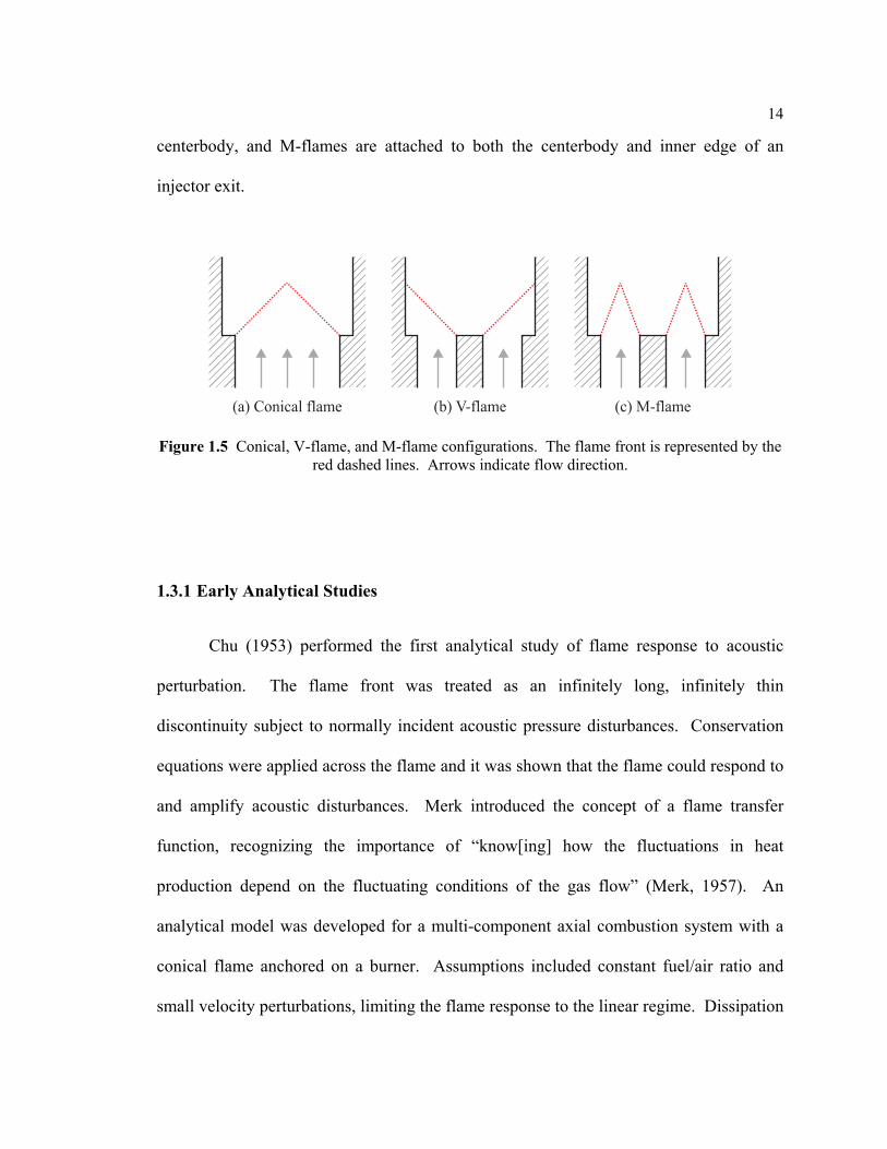
Three flame configurations, illustrated in Figure 1.5, were used in the following
reviewed studies and are referred to in the following sections. Flame configuration is
defined based on the flame attachment location relative to flow direction and the
termination location of the flame sheet. Conical flames are attached around the base
circumference of the flame, V-flames are attached only to the outer edge of an injector
14
centerbody, and M-flames are attached to both the centerbody and inner edge of an
injector exit.
Figure 1.5 Conical, V-flame, and M-flame configurations. The flame front is represented by the red dashed lines. Arrows indicate flow direction.
1.3.1 Early Analytical Studies
Chu (1953) performed the first analytical study of flame response to acoustic
perturbation. The flame front was treated as an infinitely long, infinitely thin
discontinuity subject to normally incident acoustic pressure disturbances. Conservation
equations were applied across the flame and it was shown that the flame could respond to
and amplify acoustic disturbances. Merk introduced the concept of a flame transfer
function, recognizing the importance of “know[ing] how the fluctuations in heat
production depend on the fluctuating conditions of the gas flow” (Merk, 1957). An
analytical model was developed for a multi-component axial combustion system with a
conical flame anchored on a burner. Assumptions included constant fuel/air ratio and
small velocity perturbations, limiting the flame response to the linear regime. Dissipation
(a) Conical flame (b) V-flame (c) M-flame
15
of acoustic energy was accounted for through acoustic radiation out of the combustor
exit. The primary focus was to determine the frequencies of excitation where Rayleigh’s
criterion is satisfied; however, the study did incorporate all important coupling
parameters identified in Figure 1.2 for a premixed system.
Kaskan and Noreen (1955) proposed that fluctuations in flame area due to
velocity fluctuations were the driving mechanism for heat release rate fluctuations in
premixed flames based on observations of vortex shedding from a bluff body during an
instability. Rogers and Marble (1956) used spark schlieren photographs and high-speed
video to observe vortex shedding from a flame holder edge in a rectangular combustor.
The frequency of the vortex shedding was found to occur at the combustion instability
frequency. The authors also offered the first explanation to close the feedback cycle
between pressure and heat release rate perturbations shown in Figure 1.2. Velocity
oscillations generate vortices, which entrain varying quantities of reactants, resulting in
heat release rate oscillations after a delay. These heat release rate oscillations will couple
with the acoustic pressure field in the combustor if Rayleigh’s criterion is satisfied,
feeding energy back into velocity oscillations and closing the instability cycle. The
observations of Kaskan and Noreen (1955) and Rogers and Marble (1956) initiated
numerous studies on flame-vortex interaction as the driving mechanism for premixed
flame response; several of these studies are summarized in section 1.3.2.
Markstein (1964) introduced the transport equation often used to model flame
response behavior in analytical (linear form) and simplified computational (nonlinear
form) studies. Commonly referred to as the G-equation, the equation describes the
motion of an infinitely thin flame front subject to velocity perturbations:
16
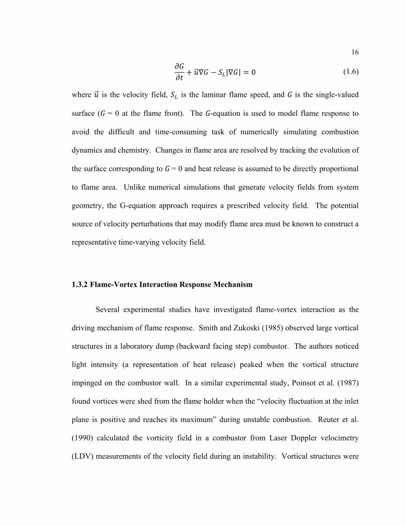
+ ∇ − |∇ | = 0 (1.6)
where is the velocity field, is the laminar flame speed, and G is the single-valued
surface (G = 0 at the flame front). The G-equation is used to model flame response to
avoid the difficult and time-consuming task of numerically simulating combustion
dynamics and chemistry. Changes in flame area are resolved by tracking the evolution of
the surface corresponding to G = 0 and heat release is assumed to be directly proportional
to flame area. Unlike numerical simulations that generate velocity fields from system
geometry, the G-equation approach requires a prescribed velocity field. The potential
source of velocity perturbations that may modify flame area must be known to construct a
representative time-varying velocity field.
1.3.2 Flame-Vortex Interaction Response Mechanism
Several experimental studies have investigated flame-vortex interaction as the
driving mechanism of flame response. Smith and Zukoski (1985) observed large vortical
structures in a laboratory dump (backward facing step) combustor. The authors noticed
light intensity (a representation of heat release) peaked when the vortical structure
impinged on the combustor wall. In a similar experimental study, Poinsot et al. (1987)
found vortices were shed from the flame holder when the “velocity fluctuation at the inlet
plane is positive and reaches its maximum” during unstable combustion. Reuter et al.
(1990) calculated the vorticity field in a combustor from Laser Doppler velocimetry
(LDV) measurements of the velocity field during an instability. Vortical structures were
17
shed in the wake of the flame holder at the instability frequency and moved at the local
convection velocity through the flame.
Schadow and Gutmark (1992) summarized experimental studies on vortex
shedding during low frequency combustion instabilities in dump and bluff-body
combustors in a review paper. They note numerous studies showed vortical structures
formed in the shear layer between the high velocity jets and lower velocity wake regions
downstream of bluff-bodies or recirculation zones formed downstream of rearward facing
step in dump combustors. Peaks in heat release were also correlated with the interaction
between vortical structures shed in multiple shear layers or in flame-wall interaction
regions. Schadow and Gutmark concluded that the main driving mechanism completing
the feedback cycle between pressure and heat release rate is the generation of vortical
structures and their interaction with the flame. Ducruix et al. (2003) separated flame
response due to vortex interaction into two mechanisms: flame area altered in the
presence of a vortex moving with the flow and vortex interaction with a boundary
resulting in a “sudden ignition of fresh material” producing a large variation in heat
release rate.
1.3.3 Controlling Parameter and Characteristic Global Response Studies
Multiple studies have been completed that focus on the controlling parameters
and characteristic global response of premixed flames. These studies provide a
framework for investigating the characteristics of the flame response and predicting the
behavior of flames based on operating condition and flame structure.
18
A numerical study by Marble and Candel (1977) of a 2D, acoustically compact V-
flame used an integral technique to solve conservation equations across a thin flame sheet
disturbed by small amplitude planar acoustic waves. The authors identified reduced
frequency ⁄ and a representation of flame angle ⁄ as two controlling
parameters of flame response ( is angular frequency, is flame length, is mean
flow velocity upstream of the flame front, and is laminar flame speed). These
parameters have been found in numerous studies since to control flame response. Values
of reduced frequency where flame response peaked (indicated by pressure fluctuations)
lead the authors to
“infer… …that the vorticity shed from the distorted flame front is such as to enhance the distortion and that when this pattern has a characteristic length that is a simple fraction of the flame length, the energy which the combustion process feeds into fluctuation of the fluid field is a maximum.”
The reduced frequency is referred to in later studies as a flow or convective Strouhal
number (St). It represents the ratio between a characteristic length of a flame ( ) and the
wavelength of a convective disturbance ( ) traveling through the flame:
= 2 (1.7)
Flame response is controlled by the ratio between these two length scales; the global
response of the flame is a strong function of the fraction or number of convective
perturbations present in the flame at any instant.
Fleifil et al. (1996) developed an analytical model of a conical laminar flame
subject to a bulk velocity oscillation. In a bulk velocity oscillation the entire flame is
modulated simultaneously by assuming the wavelength of the velocity oscillation is much
19
longer than the flame length. The authors found the “flame pattern”, or spacing of
wrinkles that develop along the flame front, are determined by a flame Strouhal number ⁄ ( is angular frequency, is pipe radius, and is laminar flame speed). At low
values of flame Strouhal number, wrinkles that perturb the flame area are eliminated by
the propagation of the flame changing the flame shape quickly to adapt to the
instantaneous velocity distribution. Therefore, during an oscillation in velocity “the
flame surface area changes accordingly and without time delay” at low flame Strouhal
numbers. The magnitude of the oscillation in flame surface area is directly proportional
to the velocity oscillation magnitude (flame transfer function gain = 1). As the flame
Strouhal number increases the flame is not capable of adjusting rapidly to the velocity
oscillation and wrinkles persist along the flame front resulting in a decrease in the
magnitude of flame response.
Baillot et al. (1992) performed an experimental study of a premixed laminar flame
subject to forced flow oscillations. A laser tomography system was used to capture
instantaneous images of the unburned gas field seeded with oil. Flame area was
determined from the edge of the unburned gas field. The experiments showed the total
flame area responded at the frequency of forcing and was deformed by waves
propagating through the flame at a speed proportional to the mean flow velocity. In
addition, the flame experienced larger relative oscillations in total area (25%) than
velocity oscillations (10%), indicating the flame is capable of amplifying inlet velocity
oscillations. Earlier analytical flame response models showed the flame acted like a low
pass filter; perturbations at low frequencies are passed unaltered while higher frequency
20
perturbations are damped in the flame’s response. These models did not capture the
potential amplification behavior of premixed flames shown in experimental studies.
Schuller et al. (2002) measured the response of a laminar premixed conical flame
to small velocity perturbations. PIV measurements in the reactants showed the velocity
perturbation traveled downstream at approximately the mean convection velocity. Axial
flame cross sections showed large coherent wrinkles generated in the flame front were
spaced at convective wavelengths associated with the mean flow velocity. Using global
CH* chemiluminescence emission to measure heat release rate, flame transfer function
gain was found to equal to unity at low forcing frequencies. In other words, the
magnitude of the heat release rate oscillation from the flame was equal to the magnitude
of the velocity oscillation imposed on the flame at low frequencies. As forcing frequency
increased, flame transfer function gain initially decreased, reached a minimum response
value, and started to increase. A convective velocity model was utilized with the G-
equation to computationally predict flame response. Bulk velocity models were shown to
be valid only for perturbations with convective wavelengths much longer than flame
(very low frequencies). Comparison between measurements and computations showed
that a convective velocity model is necessary for predicting flame response at higher
frequencies. A similar computation analysis was performed by Schuller et al. (2003) on
both laminar conical and V-flames using a convective velocity model. V-flames were
found to be more responsive to velocity perturbation than conical flames. The difference
in flame response results from the anchoring condition; a V-flame has less flame area
than a conical flame located near the anchoring point. Under the assumption that the
flame always remains anchored (valid for small velocity perturbations) the increase in
21
relative surface area of the conical flame near the attachment point limits fluctuations in
flame area. V-flames have a larger relative percentage of flame area downstream from
the anchoring point. The downstream sections of flame will experience larger variations
in position, leading to larger variations in flame area and heat release rate.
Based on the study by Marble and Candel (1977) described previously in this
section, additional analytical (Lieuwen, 2005) and experimental (Kim et al., 2009) flame
studies have identified flame structure, length, and angle as governing parameters of
global flame response. Lieuwen (2005) showed in an analytical study the response of
conical and V-flames decreased with increasing flow Strouhal number, but increased with
flame angle for fixed values of Strouhal number, demonstrating the importance of flame
structure on characteristic response.
Kim et al. (2009) found overall flame structure switched from V-flame to M-
flame as the flame as flame length decreased in an experimental study of a turbulent,
swirl-stabilized premixed natural gas and hydrogen flame. Although hydrogen
enrichment was not used during experiments covered in this dissertation, flame length
was varied by changing mixture inlet temperature, mean velocity, and equivalence ratio.
Kim et al. also showed the flame transfer function phase of turbulent flames were directly
proportional to a convective Strouhal number. In general, as flame length increases, the
time required for a velocity oscillation to travel through the flame increases relative to the
forcing period, resulting in a linear increase in flame transfer function phase.
22
1.3.4 Premixed Nonlinear Flame Response
The nonlinear flame response behavior of premixed flames has also been studied
to understand flame behavior that results in saturation of the flame response. Although
the underlying response mechanisms are identical to those present in linear response
studies, the nonlinear behavior of the flame lends insight to the processes important
during self-excited instabilities that result in limit-cycle behavior. Dowling (1997)
proposed a heat release saturation mechanism and applied a computational model to
predict limit-cycle behavior in a laminar premixed flame. The flame was modeled as an
anchored, infinitely-thin sheet perpendicular to mean flow. Heat release was directly
proportional to fuel mass flow into the flame front, which in turn was directly
proportional to flow velocity in the linear regime. If the instantaneous velocity is
negative (flow reversal), the heat release from the flame is zero. In order to maintain a
mean heat release relative to mean flow velocity, heat release is capped at twice the mean
heat release for instantaneous velocities above twice the mean velocity. The piecewise
relationship between heat release and velocity results in flame response saturation.
Results from the computation model showed nonlinear heat release response to a linear
velocity oscillation.
Lieuwen and Neumeier (2002) and Bellows et al. (2006) measured the response
of a premixed turbulent flame to velocity oscillations. Analysis of pressure signals
acquired at high forcing levels showed nonlinear flame response results from saturation
in heat release rate as acoustic processes remained in the linear regime during limit-cycle
instabilities. While liquid and solid rockets experience large relative pressure
23
fluctuations (p’/pmean ~ 50%) during instability, pressure fluctuations in lean-premixed
gas turbine systems typically peak at a few percent during limit-cycle operation. Gas
dynamic processes remain linear for small pressure fluctuations, as the pressure
fluctuations will have a negligible effect on the local speed of sound. In the
computational study previously mentioned, Dowling (1997) also showed that large
velocity and heat release fluctuations are maintained in the presence of small pressure
fluctuations.
Balachandran et al. (2005) measured the nonlinear response of a bluff-body
stabilized turbulent premixed air-ethylene flame to velocity perturbations. Flame surface
density measurements were used to image the flame front during forcing; the authors
found saturation in heat release was accompanied by the appearance of a coherent vortex
shed off the bluff-body. Although flame area increased near the vortex, imaging showed
destruction of flame area downstream of the vortex leading to saturation in overall heat
release. In addition, multiple methods for measuring heat release from a turbulent
premixed flame were tested and compared: global OH* and CH* chemiluminescence
emission, two-dimensional local OH* phase-synchronized images, flame surface density
using OH planar laser-induced fluorescence (PLIF), and local heat release rate from
simultaneous OH and CH2O PLIF. Flame surface density and the simultaneous OH and
CH2O PLIF measurements provided a direct measurement of flame area. All four
methods provided similar values for global flame response, indicating that flame area
fluctuations result in heat release rate fluctuations for premixed flames and validating the
use of chemiluminescence as a marker for heat release rate in turbulent flame studies.
24
Balachandran et al. (2008) performed an experimental study with a turbulent
premixed flame subject to imposed velocity oscillations with two harmonic frequency
components of varying magnitude. The study focused on the nonlinear regime; in
general, the addition of forcing at the harmonic frequency decreased flame response, but
also extended the linear regime to higher fundamental frequency forcing magnitudes.
Phase-locked OH PLIF was used as a direct measurement of flame area/heat release. It
was found that the presence of harmonics reduced “flame annihilation events”
(destruction of flame surface area) which reduced the magnitude of heat release
oscillations.
1.3.5 Multiple Mechanism Interaction Studies
Several analytical, computational, and experimental studies have been completed
where the combined effect of multiple flame response mechanisms on global response
was investigated. The mechanisms considered in the following studies are flame area
changes due to (i) axial velocity fluctuations, (ii) vortical structures shed from a shear
layer in the injector, (iii) swirl number fluctuations due to axial and azimuthal velocity
fluctuations, and (iv) dissipation of flame surface wrinkles due to kinematic restoration.
Although all of these mechanisms may be present in the global response of an actual
flame, each of the studies considers the interaction between only two mechanisms. Table
1.1 summarizes the approach (analytical, computational, or experimental), flow regime
(laminar or turbulent), flame response regime (linear or nonlinear) and the mechanisms
investigated in each of these studies.
25
Preetham et al. (2008) modeled laminar premixed conical and wedge-shaped
flames and found global flame response depends on local flame response to axial velocity
fluctuations and vortical structures convected by the mean flow. Axial velocity
fluctuations generate fluctuations in mean flame area, and vortical structures
simultaneously generate fluctuations in local flame wrinkling throughout the entire flame.
Global heat release response in the linear regime was found to result from a direct
superposition of the effects of both distrubances on local heat release.
Shanbhogue et al. (2009) measured the response of a bluff-body stabilized
premixed natural gas-air flame to small velocity perturbations (less than 3% of mean
velocity). Local flame response was characterized using the amplitude of the flame sheet
fluctuation over one perturbation cycle. Two distinct response regions were noted: flame
near-field and far-field. In the near-field, flame response grew with increasing axial
distance until reaching an overall maximum. Flame response was primarily controlled by
the anchoring condition in the near-field; attachment to the bluff-body prevented
significant flame movement in the flame base, limiting changes in local flame area.
Growth was attributed to vortical structures shed off the bluff-body increasing flame area.
In the far-field, flame response decayed with increasing axial distance. Dissipation of
vortical structures and flame propagation normal to itself (kinematic restoration) resulted
in a smoothing of flame surface and a reduction in heat release. Normalizing the axial
flame response by velocity oscillation magnitude showed the flame response is linear
(scales with velocity oscillation magnitude) in the near-field but nonlinear in the far-field.
This result was unexpected as other studies have shown the flame transfer function tends
to remain linear over the range of low forcing levels (1-3%) used in this study.
26
Lee et al. (2010) studied the response of a swirl-stabilized, lean-premixed
turbulent flame to small velocity perturbations (u’/umean ≈ 0.05). Phase-synchronized
CH* images showed global flame response dependence on the constructive or destructive
interaction between local flame response to axial velocity and vortical disturbances
traveling through the flame.
In a series of experimental, analytical, and computational studies, Palies et al.
(2010, 2011b, 2011c) investigated the response of a turbulent, swirl-stabilized premixed
flame to velocity forcing. The authors note the presence of a swirler adds an oscillating
azimuthal velocity component to the flow field. The combined axial and azimuthal
velocity oscillations generated oscillations in effective swirl number, flame angle, and
flame surface area near the root of the flame. In the experimental study (2010), phase-
synchronized OH* chemiluminescence emission image sets were divided into lower (near
the flame root) and upper (near the flame tip) windows and the local response of the
flame to axial and azimuthal velocity perturbations was characterized. Heat release rate
oscillations near the flame root resulted from oscillations in flame area generated by the
changes in the swirl number. Heat release rate oscillations near the flame tip were
attributed to large vortices shed from the injector exit at a peak in axial velocity. These
vortices convect with the mean flow and cause rollup of the flame tip, generating large
fluctuations in flame surface area. This study was completed with relatively high forcing
levels (u’/umean ≈ 0.5) and rollup was clearly evident in the phase-synchronized image
sets. Flame rollup appeared to be large enough to roll the flame tip near the flame base,
potentially interfering with the attempt to separate out the flame response to each
mechanism.
27
In a corresponding analytical study, Palies et al. (2011b) modeled the response of
the experimentally observed turbulent swirling flame to axial and azimuthal velocity
perturbations using the G-equation. The phase difference between the axial velocity
perturbation (traveling at an acoustic velocity) and the azimuthal velocity perturbation
(traveling at a convective velocity) was found to be an important parameter in
determining the global response of the flame.
Palies et al. (2011c) furthered this analytical study using large eddy simulation to
show that interaction between swirl number fluctuations and vortex shedding control
flame response. The flame transfer function was shown to depend on swirler location,
indicating that the phase between the swirl number fluctuation and production of vorticity
at the flame holder is a controlling parameter of global flame response.
Table 1.1 Analytical (A), computational (C), and experimental (E) studies investigating the interaction of multiple response mechanisms in premixed flames.
Authors ApproachFlow
regimeFlame response
regime Flame response driving
mechanisms
Lieuwen et al. (2008)
A,C Lam. Linear axial velocity oscillations /
vortical disturbances
Shanbhogue et al. (2009)
E Turb. Linear and nonlinear
vortical disturbances / kinematic restoration
Lee et al. (2010)
E Turb. Linear axial velocity oscillations /
vortical disturbances
Palies et al. (2010)
E Turb. Nonlinear vortical disturbances /
swirl number fluctuations
Palies et al. (2011b)
A Turb. Linear vortical disturbances /
swirl number fluctuations
Palies et al. (2011c)
C Turb. Nonlinear vortical disturbances /
swirl number fluctuations
28
1.4 Motivation, Objectives, and Outline of Dissertation
Self-excited combustion instabilities remain a serious issue hindering the
operation of lean-premixed gas turbines. Computational models are necessary in the
design and development phase to predict the stability characteristics of a combustor to
prevent expensive redesigns and modifications. To aid in the development of these
models, the underlying flame response mechanisms that control global flame response
must be characterized.
The primary focus of this work is to study the heat release rate response of a
swirl-stabilized, turbulent, lean-premixed natural gas-air flame to velocity oscillations in
an atmospheric pressure gas turbine research combustor. The specific objectives are to
(1) characterize global flame response in the linear regime based on controlling
parameters determined from stable flame structure measurements and (2) analyze the
combined influence of multiple flame response mechanisms on global flame response.
Chapter 1 provided an overview of combustion instabilities with a focus on flame
response studies pertaining to premixed gaseous fuel-air flames.
Chapter 2 gives a detailed description of the experimental setup, measurement
techniques, and data analysis procedures used in this study. The research combustor used
in this study contained an industry designed injector and the operating conditions studied
were comparable to actual gas turbine operating conditions, with the exception of mean
combustor pressure. Overall combustor length was capable of being varied, allowing for
a study of the self-excited behavior of the flame.
29
The self-excited characteristics of the combustor are discussed in chapter 3, along
with criteria used to define stable and unstable combustor behavior. In chapter 4, stable
flame images are used to quantify several characteristic parameters of turbulent flame
structure previously reported as controlling parameters of flame response.
In chapter 5, a comparison is made between self-excited and forced flame
response. Flame response is quantified throughout this dissertation using the flame
transfer function concept discussed in section 1.2.1.3. In self-excited experiments
velocity oscillations occurred naturally as part of the instability cycle, where as forced
experiments required the use of a siren to introduce velocity oscillations at known
frequencies and magnitudes. A comparison is also made for each of the coupling
relationships described in section 1.2.1 between self-excited and forced flames and
potential saturation mechanisms for limit-cycle oscillations are discussed.
Global flame response behavior across a wide range of operating conditions is
discussed in chapter 6. Multiple controlling parameters defined in previous studies are
examined to determine the dominant driving mechanism of flame response in this study.
The response of the flame is also examined as two separate components, one long
wavelength acoustic component and a separate convective component. In chapter 7,
phase-synchronized flame imaging is used to quantify local oscillations in heat release
rate. Evidence of flame response to axial velocity oscillations and vortical disturbances is
observed in the image sets.
Chapter 2
Experimental Techniques
The experimental techniques used in this study are discussed in this chapter. The
experimental setup is described in section 2.1 and instrumentation is discussed in section
2.2. Data analysis is divided into two sections. Processing related to one-dimensional
time-varying signals is discussed in section 2.3 while image processing techniques are
described in section 2.4.
2.1 Experimental Setup
All measurements were completed in an atmospheric, variable-length, lean-
premixed research combustor with a single industrial gas turbine injector. Although
termed atmospheric, combustion occurs in an enclosed chamber to prevent equivalence
ratio fluctuations due to external air entrainment. Actual mean pressure in the combustor
chamber was approximately one psig due to restrictions in the downstream section. An
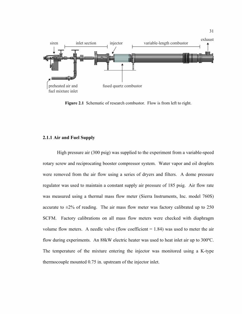
overall view of the experimental setup is provided in Figure 2.1. The primary
components of the system include an air heater, siren, inlet section, injector, fused quartz
combustor, variable-length combustor, and exhaust system. The overall length of the
experiment was approximately three meters.
31
Figure 2.1 Schematic of research combustor. Flow is from left to right.
2.1.1 Air and Fuel Supply
High pressure air (300 psig) was supplied to the experiment from a variable-speed
rotary screw and reciprocating booster compressor system. Water vapor and oil droplets
were removed from the air flow using a series of dryers and filters. A dome pressure
regulator was used to maintain a constant supply air pressure of 185 psig. Air flow rate
was measured using a thermal mass flow meter (Sierra Instruments, Inc. model 760S)
accurate to ±2% of reading. The air mass flow meter was factory calibrated up to 250
SCFM. Factory calibrations on all mass flow meters were checked with diaphragm
volume flow meters. A needle valve (flow coefficient = 1.84) was used to meter the air
flow during experiments. An 88kW electric heater was used to heat inlet air up to 300ºC.
The temperature of the mixture entering the injector was monitored using a K-type
thermocouple mounted 0.75 in. upstream of the injector inlet.
siren inlet section
preheated air and fuel mixture inlet
fused quartz combustor
injectorexhaust
variable-length combustor
32
A fuel manifold supplied natural gas (approximately 95% methane) to the
experiment. A series of gas regulators and a heater were used to prevent excessive
cooling of the natural gas during sudden expansions. Gas flow was metered to the
experiment at 200 psig using a needle valve and mass flow rate was measured using a
thermal mass flow meter (Teledyne Hastings 300 Series). A series of baffles encouraged
mixing and a choked inlet to the combustor prevented pressure oscillations from varying
the fuel flow rate.
2.1.2 Injector Design
The industrial injector used in this study was a Solar Turbines, Inc. production
model used in the Taurus 70 (T70) line of combustors. The T70 is a dry lean-premixed
low emission combustor used for electric energy production, gas compression, or liquid
pumping with a maximum rated electric power output of approximately 7.5 MW. In the
actual gas turbine twelve injectors are arranged in an annular configuration around a
section of the injector. Minor modifications were made to the barrel and main fuel
manifold to allow for measurement access.
A single axial swirler generates an azimuthally swirling flow, enhancing flame
stabilization. The swirling flow induces a low pressure central region in the combustor,
generating an inner recirculation zone to entrain burnt products near the centerbody face
that mix with fresh reactants to stabilize the flame (Lefebvre, 1999). A recessed
33
centerbody provides an anchoring location for the main flame and an additional flow
passage for a pilot flame.
Figure 2.2 Schematic of injector geometry and pressure transducer locations.
Two flow paths are available through the injector: main and centerbody. Under
actual field operation air is split between the two paths with approximately 5% of the
total air flow entering through the centerbody. Centerbody air is used to cool the
upstream face of the centerbody exposed to the combustor and supply air for a pilot
flame. Pilot flames are secondary higher equivalence ratio premixed flames or diffusion
flames used for stabilization during actual gas turbine operation (Karim et al., 2003). In
this study fuel and air were premixed well upstream (L/D ≈ 50) of the injector; the
main flame
secondary flame
swirler
combustor pressure transducer port
upstream pressure transducer port
downstream pressure transducer port fused quartz tube
dump plane
main air/fuelmixture
main air/fuelmixture
secondary air/fuelmixture
centerbody
dumpplate
34
mixture flowed through the air line used for the pilot flame resulting in a secondary flame
with the same equivalence ratio as the main flame during all measurements.
A stainless-steel dump plate was mounted flush with the injector barrel exit. The
dump plate was water-cooled to prevent warping and contained an access port for
combustor pressure measurement. Two access ports (upstream and downstream) for
pressure transducers were machined into the outer casing of the injector body to allow
pressure measurement in the main mixture flow. The pressure signals from the upstream
and downstream transducers were used to calculate velocity fluctuations (section 2.3.3).
2.1.3 Optically-accessible Combustor
A fused quartz tube (type GE 214, inner diameter = 150 mm, wall thickness = 3
mm, length = 305 mm) provided complete optical access for global chemiluminescence
emission measurement and flame imaging. The ends of the tube were secured to the
dump plate and a water-cooled transition section using high-temperature RTV-silicone.
An additional port in the dump plate allowed access for ignition fuel and high voltage
spark igniter used to ignite a diffusion flame during startup.
The external surface of the quartz tube was actively cooled with room
temperature air supplied by a cooling ring positioned concentric with the tube. Static
pressure inside the combustor was measured using a digital static pressure gauge (Omega
model DPG1000B-05G) and varied between 0.7 psig and 1.6 psig depending on
operating condition.
35
2.1.4 Variable-length Combustor
Overall combustor length can be continuously varied between 18 in. and 60 in.
using a plug centered in a double-wall stainless steel combustor section. Combustor
length is defined as the distance between the downstream end of the dump plate (the
dump plane) and base of the plug head (Figure 2.3). Changing the combustor length
alters the frequency of acoustic modes and mode shape of the overall system, enabling
the system to be tuned to ensure stable combustion during stable flame imaging and
forced flame response measurements. The plug consisted of a stainless steel cone-shaped
head cooled with distilled water flowing through channels behind the upstream face. The
water was then sprayed on the back of the head for additional cooling. Distilled water
was used to prevent precipitation fouling at the high temperatures found downstream of
the flame. A pump elevated the water pressure to approximately 150 psig in the plug to
increase flow through the spray nozzles and raise the boiling point of the water to prevent
vaporization within the plug head.
Figure 2.3 Schematic of fused quartz and variable-length combustors.
combustor length (Lc)
fused quartz combustor
dump plate
moveable plug
double-walled variable-length combustor
water-cooled transition section
water spray
cooling air
cooling air
36
The plug cone rested on two Kovar alloy bearings and was moved using a
horizontal translation table driven by a computer controlled stepper motor. Combustion
products from the flame flowed between the plug head and inner wall of the double-
walled stainless steel combustor section (~89% reduction in area). The double-walled
combustor section was comprised of two concentric stainless steel pipes. Room
temperature air flowed between the tubes to actively cool the inner tube. Mufflers were
used on the main and cooling air exhausts to reduce noise.
2.1.5 Siren
A rotor-stator siren was used to modulate the mixture flow during forcing
measurements. The rotor was driven by a brushless DC motor (VEXTA model
BLFM6400-A). Modulation frequency was set using a digital motor driver (VEXTA
model BLFD400S2) with feedback control attached to the DC motor. Feedback control
maintained the set driving frequency to within one hertz during forcing. The maximum
modulation frequency was 500 Hz.
Two globe valves were used to varying the amount of flow through the siren,
allowing for control of the modulation level. In general, the maximum achievable
modulation level decreased with increasing modulation frequency. An incremental
encoder (BEI model H25) connected to the siren drive shaft provided a trigger signal
used during phase-synchronized imaging of forced flames.
37
Figure 2.4 Siren and valves used to control forced velocity oscillation.
2.2 Instrumentation and Measurement Techniques
2.2.1 Data Acquisition
Pressure and global chemiluminescence signals were recorded nearly
simultaneously (one microsecond delay between signal acquisitions) using a National
Instruments PCI-6259 data acquisition board with a BNC-2110 connector block. All
self-excited and global FTF measurement signals were recorded with a sampling rate of
fs = 8192 samples/second for 8 or 32 seconds. The records were then divided into one-
second long sets (N = 8192 samples) and each set was processed separately, leading to a
final frequency resolution of Δf = 1 Hz. A LabVIEW interface was used to manage data
recording and allowed for near real-time views of all signals.
preheated air and fuel mixture inlet
sirenmotor
siren valve
bypass valve
38
2.2.2 Pressure Oscillation Measurement
Pressure measurements served two primary purposes: characterize the magnitude
of self-excited combustion instabilities (combustor pressure transducer) and measure
pressure fluctuations to calculate velocity fluctuations using the two-microphone method
(upstream and downstream transducers) The two-microphone method (TMM) is
discussed in section 2.2.3. The piezoelectric pressure transducers used were PCB model
112A22 (integrated charge converter) and model 112A04 (separate inline charge
converter). All transducers were water cooled and recessed mounted to prevent
overheating. The voltage outputs of all converters were amplified by a factor of ten using
a PCB model 482A16 signal conditioner.
2.2.3 Global Heat Release Rate Measurement
An accurate measurement of heat release rate is needed to quantify the flame’s
response to velocity perturbations. Global chemiluminescence emission has been used in
numerous flame studies based on experiments that show that for a fixed fuel lean
equivalence ratio, global chemiluminescence is directly proportional to fuel mass flow
and heat release rate (Clark, 1958; Hurle et al., 1968; Lee et al, 2005). In this study, CH*
chemiluminescence emission was measured using a photomultiplier tube (PMT) with a
432 ± 5 nm band-pass filter and series of lenses to focus the emission onto the detector.
In addition to simplicity, global chemiluminescence has shown good agreement with
more complex global measurements of heat release rate and local measurements of flame
area (Balachandran et al., 2005).
39
2.2.4 Flame Imaging
Two-dimensional CH* chemiluminescence emission images were acquired to
characterize flame shape, structure, and changes in spatial and temporal heat release
distribution during forcing measurements. Images were acquired using a 430 ± 5 nm
filtered intensified charge-coupled device (ICCD) camera. Raw images are projection
(line-of-sight) views of CH* chemiluminescence emission from the flame. Assuming
axisymmetric flow, a discrete inverse Abel transform (Dasch, 1992; Alvarez et al., 2002)
can be applied to the raw images to extract an axial cross-section (section 2.4.2). Flame
image acquisition was sub-divided into two types based on the purpose of the
measurement: stable/time-averaged imaging and phase-synchronized imaging.
2.2.4.1 Stable and Time-averaged Flame Imaging
Stable and time-average flame images represent average flame position and
shape. The images were acquired using a Princeton Instruments model 576G ICCD
camera with a 60 mm f/2.8 Nikkor lens operating in “Shutter” mode. The images were
acquired with low gain, long exposure time, and multiple accumulations. Low gain was
used to decrease noise amplification associated with high gains. Long exposure times
and multiple accumulations allowed for increased signal acquisition. Figure 2.5 shows
examples of (a) stable and (b) time-averaged projection images acquired at the same
operating condition. Stable and time-averaged refer to the nature of the flame under
study; the measurement technique is identical during both measurements.
40
Figure 2.5 Examples of stable (a) and time-averaged (b) flame projection images (operating condition: Tin = 250°C, umean = 40 m/s, φ = 0.65). The faint hexagons present in both images result from the fiber optic bundles in the camera that connect the intensifier to the CCD. Both
images are self-scaled. Radial and axial distances are in centimeters.
A pseudo self-scaled colormap is applied to each image. Black/cool colors
represent areas with lower heat release rate than white/warm colors. Self-scaled indicates
the colormap of each image is scaled to the minimum and maximum intensities present
only in the image. A comparison in intensity between separate images requires a shared
colormap. The smaller secondary flame anchored on the pilot hole edge is visible in both
images. The widening of the flame brush in the time-averaged image is due to the
presence of velocity fluctuations ( = 0.20⁄ ) higher than background turbulent
Phase-synchronized images were acquired using a Princeton Instruments PI-MAX
ICCD camera (model 7467-0008) with a 50 mm f/1.8 Nikkor lens. The images show the
temporal and spatial evolution of heat release during forced flame measurements. All
images were acquired with an exposure time of 1 24⁄ the forcing period, high gain, and
sixty accumulations. The relatively short exposure times (50-350 μs) were necessary to
approximate the instantaneous heat release distribution of the flame at multiple phases
within one cycle. Due to the short exposure time, high gain was required to amplify
chemiluminescence emission from the flame and sixty accumulations further increased
the signal. Figure 2.6a shows an example of a projection image set acquired at twelve
phase angles during a forcing experiment. Figure 2.6b shows the corresponding relative
velocity and global heat release rate oscillations versus phase angle at the forcing
frequency of 120 Hz. PMT and ICCD measurements of heat release rate are shown and
agree within a few percent.
The camera was triggered off an incremental encoder attached to the siren. The
encoder provided a clean trigger signal to ensure accumulations are captured at the
correct phase angle within a cycle. However, the trigger signal from the encoder does not
necessarily correspond to distinct part of the forcing cycle and a delay was added to the
encoder signal to account for the phase difference between the encoder and velocity at the
TMM. The delay was determined from a measurement prior to the recording of phase-
synchronized image data and was checked during the measurement at each phase angle to
ensure no variation in the delay occurred.
42
(a)
(b)
Figure 2.6 (a) Phase-synchronized smoothed projection image set example. Images are all scaled to the maximum intensity in the 330° image. (b) Corresponding relative TMM velocity
(–––) and global heat release rate oscillations from PMT measurement filtered at 120 Hz (– – –), ICCD measurement filtered at 120 Hz (), and unfiltered ICCD measurement (). Operating
condition: Tin = 250°C, umean = 30 m/s, φ = 0.60, forcing frequency = 120 Hz, u’rms/umean ≈ 0.07.
Increasing intensity
0º 30º 60º 90º
120º 150º 180º 210º
240º 270º 300º 330º
Phase angle [deg.]
0 30 60 90 120 150 180 210 240 270 300 330 360
u'rm
s/um
ean
and
q'rm
s/ qm
ean
0.85
0.90
0.95
1.00
1.05
1.10
1.15
··
43
2.3 Pressure, Velocity, and Global Chemiluminescence Signal Analysis
The numerical techniques used to analyze one-dimensional time-varying discrete
data are discussed in the following sub-sections. Sections 2.3.1 through 2.3.3 cover
techniques used to analyze raw signals while sections 2.3.4 and 2.3.5 describe the
techniques used to determine the coherence between signals and the uncertainty in linear
fits respectively.
2.3.1 Linear Spectrum and Single-sided Power Spectral Density
Pressure, velocity, and chemiluminescence signals were analyzed in the
frequency-domain to characterize response at or near the perturbation frequency. A Fast-
Fourier Transform (FFT) was used to calculate a signal’s linear spectrum:
= ∆ (2.1)
where a is the time-domain quantity of interest, Δt is the time between acquired samples,
A is the linear spectrum of a, k is the frequency-domain index, i is the index of the time-
domain sample, j is the imaginary unit, and N is the number of samples. The phase of the
perturbation was determined from the angle between the real and imaginary component
of the linear spectrum at the frequency of interest. The signal’s single-sided power
spectral density (SSPSD) was then calculated from the linear spectrum and Parseval’s
theorem was used to calculate fluctuation magnitudes. The single-sided power spectral
density is given by the piecewise function:
44
≡ 1 | | for = 0
(2.2)≡ 2 | | for1 ≤ ≤ 2 − 1
≡ 1 ⁄ for = 2
where a is the time-domain quantity of interest, T is the period of the acquired signal, A is
the linear spectrum of a, k is the frequency-domain index, and N is the number of
samples. Parseval’s theorem relates the root-mean-square (rms) magnitude of a signal in
the frequency-domain to the magnitude of a signal in the time-domain:
( ) = ( ) ∙ ∆ (2.3)
where k is the index of the bin corresponding to the frequency of interest, arms(k) is the
corresponding time-domain rms magnitude of a at the frequency of interest, Gaa(k) is the
single-sided power spectral density value, and Δf is the frequency resolution (Mitra,
2006). Parseval’s theorem allows for the magnitude of oscillations at a single frequency
to be isolated from background noise. The pressure field in the combustor used in this
study contains relatively high oscillations across multiple frequency ranges due to the
turbulent nature of the flow and oscillations at the desired frequency must be isolated to
remove the effect of background noise on oscillations.
2.3.2 Forced and Self-excited Flame Signal Analysis Comparison
During forcing measurements, the frequency of the velocity oscillation generated
by the siren was controlled to within a hertz using the controller described in section
45
2.1.5. However, during self-excited measurements, an unstable flame coupled with
system acoustics and the dominant frequency of oscillation must be determined from
pressure, velocity, or chemiluminescence spectra. To account for uncertainty in the exact
frequency of oscillation, a modified version of Parseval’s theorem that incorporates
summing near the peak frequency was used to represent the oscillation magnitude:
( ) = ( ) ∙ ∆ (2.4)
If the oscillation frequency does not correspond to the center bin frequency, energy will
spread to nearby bins as a result of the analysis procedure (leakage). In addition, the
actual oscillation frequency was most likely not constant during the time required to
record a signal, resulting in energy spread throughout several bins. During the forcing
measurements, oscillation frequency was held constant using a controller with feedback
that maintains the forcing frequency to within one hertz.
Figure 2.7 shows an example of a typical single-sided power spectral density for
self-excited and forced flame CH* chemiluminescence signals. Pressure and velocity
spectra are similar. The self-excited spectra (a) shows the 171 Hz bin contains the
highest magnitude oscillation, with additional, smaller magnitude oscillations spread
across nearby bins. The forced spectra (b) shows a single oscillation contained within the
bin corresponding to the forcing frequency of 170 Hz. Summing the magnitude of the
oscillations in bins within ±5 Hz of the dominant frequency results in similar CH*
chemiluminescence fluctuation magnitudes. A comparison between self-excited and
forced flame response is made in chapter 5 to check the validity of the forced response
46
measurement. If the differences in signal processing described above are not accounted
for in the analysis of signals from the two different measurements any observed
disagreement may be due to processing technique instead of actual physical differences
between measurements.
Figure 2.7 CH* single-sided power spectral densities for forced (a & b) and self-excited (c & d) flames. Operating condition: Tin = 250°C, umean = 40 m/s, φ = 0.65, u’rms/umean = 0.10 (forced),
LC = 18 in. (self-excited).
0 100 200 300 400 500
CH
* S
SP
SD
[a.
i.u./ √
Hz]
0.00
0.05
0.10
0.15
0.20
0.25
0 100 200 300 400 500
CH
* S
SP
SD
[a.
i.u./ √
Hz]
0.00
0.05
0.10
0.15
0.20
0.25
Frequency [Hz]
155 160 165 170 175 180 185
CH
* SS
PSD
[a.
i.u./ √
Hz]
0.00
0.05
0.10
0.15
0.20
0.25
Frequency [Hz]
155 160 165 170 175 180 185
CH
* SS
PSD
[a.
i.u./ √
Hz]
0.00
0.05
0.10
0.15
0.20
0.25
(a) (c)
(b) (d)
47
2.3.3 Two-microphone Method for Calculating Velocity Oscillations
Velocity oscillations near the base of the flame must be determined to provide an
input fluctuation (u’) for the premixed flame transfer function. Several methods exist to
measure velocity, including hot-wire anemometry and laser-doppler velocimetry (LDV).
Hot-wire anemometry could not be used due to the elevated inlet mixture temperature (>
200°C) and LDV would have required additional optical access in the injector barrel and
particle seeding. In addition, a single hot-wire or LDV measurement provides a point
velocity measurement at a single radial location while an average axial velocity
oscillation across the injector radius is needed. To eliminate the problems associated
with hot-wire anemometry and LDV, the two-microphone method was used to calculate
velocity oscillations from pressure measurements (Waser and Crocker, 1984).
Two pressure transducers separated by 1.25 in. were used to measure an axial
pressure gradient, assuming a finite difference approximation. The two pressure
transducers were recessed mounted in the outer wall of the injector between the swirler
and injector exit, as shown in Figure 2.2. Assuming incompressible, inviscid flow and
neglecting body forces, particle acceleration is related to the axial pressure gradient using
Eq. 2.5, a linearized form of conservation of momentum for flow in the x-direction:
+ 1 = 0 (2.5)
where u is axial velocity, p is pressure, and ρ is mixture density (Waser and Crocker,
1984). Although the natural gas-air mixture is compressible, the incompressible
assumption is valid for flows at low Mach numbers. The maximum Mach number of
operating conditions tested is approximately 0.14, less than the critical Mach number of
48
0.3 recommended for an incompressible flow assumption (Anderson, 1991). In addition,
pressure oscillations during combustion instabilities are typically only a few percent,
producing negligible density oscillations. The Reynolds number of the flow inside the
injector is relatively high (approximately 15,000-25,000 based on the range of mean
velocities and injector annulus height) for the operating conditions tested, indicating
inertial effects are much larger than viscous effects and permitting the use of the inviscid
assumption (Acheson, 1990). No body forces act in the axial flow direction. It also must
be assumed spatial variations in the axial, azimuthal, and radial velocity components are
negligible between the two microphones to remove the convective acceleration term and
yield a relationship between unsteady acceleration ( ⁄ ) and pressure gradient.
Finally, several studies (Balachandran, 2005; Lee, 2009a) compared axial velocity
magnitude and phase values between two-microphone and hot-wire anemometry
measurements in injectors similar to the one used in this dissertation. Both studies found
good agreement between the measurement techniques for frequencies up to 500 Hz,
supporting the use of the technique in similar gas turbine injector studies.
Applying the finite difference approximation and Fourier transform to Eq. 2.5
yields Eq. 2.6:
= −∆ (2.6)
where U is the velocity linear spectrum, Pds and Pus are the pressure linear spectrums of
the downstream and upstream locations respectively, ω is angular frequency, ρ is mixture
density, Δx is the spacing between the transducers, and j is the imaginary unit (Waser and
Crocker, 1984). Example upstream pressure (a), downstream pressure (b), and velocity
49
(c) single-sided power spectral densities from a forced flame experiment are shown in
Figure 2.8. The mixture was forced at 200 Hz and the siren and bypass valves were
adjusted to produce an oscillation magnitude u’rms/umean = 0.05 at the TMM location. The
spectra shows pressure oscillation magnitudes at 200 Hz approximately equal to 0.03 psi,
approximately an order of magnitude above background pressure oscillations at other
frequencies.
The velocity linear spectrum calculated using Eq. 2.6 is complex, but does not
estimate the mean flow velocity. Mean velocity was calculated using the geometric open
area of the nozzle at the two-microphone location, density of the mixture, and
measurement of total mass flow. Densities were calculated from temperature and static
pressure measurements assuming ideal gas behavior.
2.3.3.1 Frequency Limits of the Two-microphone Method
The two-microphone method is subject to both lower and upper frequency limits
(Waser and Crocker, 1984). As frequency decreases, the acoustic wavelength of the
pressure perturbation increases and the actual pressure gradient between the upstream and
downstream pressure transducers is reduced. Calculated particle velocity will be
inaccurate if the actual difference in pressure between transducers is comparable to
pressure fluctuations associated with turbulence. The velocity single-sided power
spectral density in Figure 2.8c illustrates this limit; as frequency decreases towards zero,
the velocity magnitude increases asymptotically.
50
Figure 2.8 Upstream pressure (a), downstream pressure (b), and velocity (c) single-sided power spectral densities. Operating condition: Tin = 250°C, umean = 50 m/s, φ = 0.55, u’rms/umean = 0.05.
The upper frequency limit results from error in the finite-difference
approximation at short wavelengths. As frequency increases the acoustic wavelength will
become comparable to the transducer spacing, resulting in a poor finite-difference
approximation (Thompson and Tree, 1981). However, the upper frequency is limited to
0 100 200 300 400 500 600 700
US
Pre
ssur
e S
SP
SD
[psi
/ √H
z]
0.00
0.01
0.02
0.03
0.04
0 100 200 300 400 500 600 700
DS
Pre
ssur
e S
SP
SD
[psi
/ √H
z]
0.00
0.01
0.02
0.03
0.04
Frequency [Hz]
0 100 200 300 400 500 600 700
Vel
ocit
y S
SP
SD
[m/s
/ √H
z]
0.0
0.5
1.0
1.5
2.0
2.5
3.0(c)
(b)
(a)
51
500 Hz during forcing by the siren used to modulate the mixture and the highest
frequency self-excited instability observed was approximately 600 Hz. At 600 Hz, the
1.25 in. spacing between upstream and downstream transducers is less than 5% of the
wavelength of an acoustic oscillation, well within the upper frequency limit of the two-
microphone method.
2.3.4 Coherence and Single-sided Cross Spectral Density (SSCSD)
Turbulent fluctuations in the combustor lead to noisy pressure, velocity, and
chemiluminescence signals. In order for the flame transfer function to accurately
quantify the flame’s heat release rate response to velocity oscillations, the two signals
must be highly related, otherwise noise present in the system may corrupt the
measurement. In addition, pressure signals at the upstream and downstream pressure
transducers must be highly associated for the two-microphone method to provide an
accurate measurement of particle velocity (Seybert and Soenarko, 1981). The level of
association was quantified in this study using the spectral coherence (or coherence)
between two signals. Coherence provides an estimate for the causality between two
signals provided the relative phase between signals is stable. The coherence between
two signals was calculated using:
= ̅∗ ̅̅ ̅ (2.7)
where a and b are the time-domain signals compared, ̅ and ̅ are the mean single-
sided power spectral densities (Eq. 2.2) of a and b over multiple records respectively, ̅
52
is the mean single-sided cross-spectral density (SSCSD) of a and b over multiple records
(Eq. 2.8), and ̅ ∗ is the complex conjugate of the single-sided cross spectral density of a
and b (Mitra, 2006).
The single-sided cross-spectral density needed to calculate coherence is given by:
≡ 1 ∗ for = 0
(2.8) ≡ 2 ∗ for1 ≤ ≤ 2 − 1
≡ 1 ⁄∗ ⁄ for = 2
where T is the period of the acquired signals, A and B are the linear spectrum of a and B,
k is the frequency-domain index, and N is the number of samples.
Multiple records of each signal are required to calculate coherence as the
steadiness of the relative phase between signals must be determined. Low coherence may
result from either random fluctuations in the combustor producing unrelated signals or
changes in the relative phase between signals over time.
2.3.5 Uncertainty in the Slope of a Linear Fit
In the linear regime, the slope of the relative heat release rate response versus
relative velocity fluctuation magnitude yields the gain of the flame transfer function
(Figure 1.4). Simple linear regression was used to find the slope and intercept of a line
of best fit (Taylor, 1997). The relative uncertainty in the slope was calculated using:
53
( )| | = √√ − 2 (2.9)
where a is the slope of the line of best fit, σ(a) is the absolute uncertainty of the slope, R2
is the coefficient of determine of the linear fit, and N is the number of samples used in the
linear fit (Higbie, 1991). Determination of the uncertainty was necessary to compare
results from self-excited and forced experiments in Chapter 5.
2.4 Flame Image Processing
This section details the procedures and algorithms used to process flame image
data for stable, time-averaged, and phase-synchronized images. After a discussion of the
inverse Abel transform used in this study, the procedure used to process all images is
listed, followed by definitions of several metrics used to quantify the flame’s structure
and local heat release rate response.
2.4.1 Forward and Inverse Abel Transforms
An inverse Abel transform was applied to all acquired projection images.
Projection images ( , ) are line-of-sight integrated views of the flame’s
chemiluminescence emission. Assuming the flame’s emission is axisymmetric, applying
an inverse Abel transform yielded an emission image ( , ), a two-dimensional,
infinitely thin axial cross-section of the emission distribution from the flame.
54
The Abel transform was discovered by Niels Henrik Abel (1802 – 1829) in 1826.
Although used to analyze axisymmetric image data in modern times, the Abel transform
was discovered in pursuit of a general solution to the tautochrone problem. A
tautochrone is a special curve that results in a constant travel time independent of starting
position for objects sliding along the curve subject to a uniform gravitation field
(assuming zero friction). The tautochrone was researched in an attempt to improve the
consistency of timekeeping devices. Abel generalized the problem to find the equation of
the curve that results in a given travel time as a function of starting height, discovering
the first integral transform in the process (Simmons, 1991). The inverse Abel transform
is given by (Abel, 1826; translated by Tamarkin, 1959):
( ) = − 1 ′( )√ − (2.10)
where ( ) is the emission intensity at radial location and ( ) is the projection
intensity at location . If experimental data were fitted by analytical functions, Eq. 2.10
could be used to directly integrate the analytical expression to yield the emission values.
In this study the acquired projection data were discrete and did not conform to a
Gaussian, polynomial, or other simple function that can be easily differentiated and
integrated. A discrete form of the inverse Abel transform was necessary to transform
the projection images.
55
2.4.2 Discrete Inverse Abel Transform Algorithm
Discretization of Eq. 2.10 results in two difficulties inherent in most discrete
inverse Abel transforms that may result in inaccurate transforms or increased noise in the
emission image (Dasch, 1992; Yuan, 2003):
1. the integrand is undefined at = 2. the first derivative of the projection data ′( ) must be approximated from
discrete data
To avoid the discontinuity present in the integrand at = the inverse Abel transform
can be performed in the frequency-domain using a Hankel-Fourier algorithm (Álvarez et
al., 2002). Projection-slice theorem (also referred to as Fourier slice theorem) states that
for a 2D axisymmetric function the zeroth-order Hankel transform ( ) of that function is
equivalent to applying an Abel transform ( ) followed by a Fourier transform ( ): = (2.11)
Hankel-Fourier algorithms first apply a Fourier transform to the projection data followed
by an inverse Hankel transform to yield the inverse Abel transform (Bracewell, 1956):
= (2.12)
The discrete form Hankel-Fourier inverse Abel transform used in this study is given by
(Álvarez et al., 2002):
= 12 [(2 + 1)∆ ] ( ) cos 2 + 1 2 + 1 (2.13)
where ( ): calculated emission value at radial location : number of samples in one half of the projection vector ∆ : spatial spacing between projection values ( ): projection value at location : zero-order Bessel function of the first kind
56
The inverse Abel transform is one part of the procedure used to calculate emission
data from projection data described in the following section.
2.4.3 Image Processing Procedure
The procedure used to extract emission data from projection data was similar for
stable, time-averaged, and phase-synchronized images:
1. Eight (stable or time-averaged flames) or sixty (phase-synchronized flames) images were acquired at a specific exposure time and camera gain. Camera exposure time was limited to several hundred microseconds for phase-synchronized measurements and sixty images were required to achieve reasonable signal levels. Stable and time-averaged flame measurements were made with exposure times of several hundred milliseconds and fewer images were necessary to resolve the flame. The images were then summed to yield a single raw image
2. At the end of the experiment, eight or sixty images were acquired with identical
camera settings but without combustion. The images were then summed to yield a single background image
3. The background image was subtracted from the raw image
4. Regions outside of the fused quartz combustor were cropped out of the
background-subtracted image
5. The cropped image was averaged across the combustor centerline
6. A moving-average filter (5 × 5) was applied to the averaged image to reduce noise
7. The inverse Abel transform was applied to the smoothed image column by column to produce the corresponding emission image
Figure 2.9 shows example (a) raw and (b) background-subtracted averaged projection
images along with the final emission image with two different color scales (c & d).
57
Figure 2.9 Image processing procedure. Projection images (a) are background subtracted and averaged across the combustor centerline (b). After applying a moving average filter, a discrete inverse Abel transform is applied to each column to yield an emission image (c). Weighting the
emission image by the peak intensity in the main flame allows for easier visualization of the main flame’s structure (d). Images are self-scaled. Radial and axial distances are in centimeters.
(a) Projection image (b) Background subtracted and averaged projection image
(c) Emission image (d) Emission image scaled to maximum intensity in main flame
7.56.0
4.0
2.0
0.0
2.0
4.0
6.07.5
0 2 4 6 8 10 12 14
7.56.0
4.0
2.0
0.0
2.0
4.0
6.07.5
0 2 4 6 8 10 12 14
7.56.0
4.0
2.0
0.00 2 4 6 8 10 12 14
7.56.0
4.0
2.0
0.00 2 4 6 8 10 12 14
Increasing intensity
main flame
secondary flame
main flame
secondary flame
58
2.4.4 Processed Image Analysis Methods
After the emission image has been calculated, several processes were used to
calculate metrics used to define flame structure and shape. The equations, calculation
procedures, and example images are discussed in the following sections.
2.4.4.1 Mean flame sheet
Based on the exposure time and averaging required to image the flame, an
instantaneous “snapshot” of the flame sheet was not possible. In addition, the flame is
highly turbulent and any single representation of the flame sheet location may not be
useful in characterizing the flame’s structure. All of the resulting emission images
showed a flame brush, or the extent and distribution of the flame sheet movement within
the combustor. The intensity of any pixel in the image is related to the residence time of
the flame sheet in that specific location and the emission image shows the heat release
distribution in the combustor, not the location of the flame sheet.
A mean flame sheet location was extracted by selecting the pixel of maximum
intensity in each column in both the main and secondary flames. An example is shown in
Figure 2.10. The black line through the center of each flame is the location of the mean
flame sheet. The turbulent nature of the flame excludes this mean flame sheet from
accurately representing the flame area at any instant; however, the mean sheet is useful in
determining changes in the location of the flame and flame angle during velocity
oscillations.
59
Figure 2.10 Mean flame sheet location (black line) in the main and secondary flames. The image is scaled to the maximum intensity in the main flame. Radial and axial distances are in
The emission image is infinitely thin and does not account for the radial
distribution of heat release from the flame. To represent the location and magnitude of
heat release in context of the combustor, the emission images were radially weighted to
yield “revolved” images that account for the circumferential heat release distribution
from the flame. While a revolved image does not physically represent the location of
heat release in a slice of the flame, it does provide a better representation of the location
of heat release relative to the injector. Figure 2.11 shows an example of an emission
image (a) and the corresponding revolved image (b). Revolved images were produced by
multiplying each pixel in an emission image by 2 , where is the radial distance from
the pixel to the combustor centerline.
main air/fuel
7.5
6.0
4.0
2.0
0.00 2 4 6 8 10 12 14 16 18
centerbody
dumpplate
combustor centerline
secondary air/fuel
fused quartz tube
main flame
secondary flame
60
Figure 2.11 Examples of emission (a) and revolved (b) flame images. Images are self-scaled. Radial and axial distances are in centimeters. Operating condition: stable flame, Tin = 250°C,
umean = 40 m/s, φ = 0.65.
2.4.4.3 Flame center-of-heat release (CoHR), length (LCoHR), and width (WF)
Numerous studies (summarized in section 1.3.3) have shown that flame response
is partially controlled by a characteristic flame length. In laminar conical flame studies
the characteristic flame length is typically the length of the flame from base to tip. In
turbulent flame studies, especially those that involve interaction with a boundary, the
downstream “end” of the flame is not clearly defined. However, turbulent flame studies
(Kim et al., 2010; Ranalli et al., 2011) have used a characteristic distance between the
flame anchoring point and a location of significant heat release. In this study, the flame’s
center-of-heat release (CoHR) represents the location of largest heat release. Although
similar to the location of maximum heat release, the center-of-heat release calculation
uses the intensity and location of multiple pixels in a weighting function to generate a
(a) Emission image (b) Revolved image
Increasing intensity
7.56.0
4.0
2.0
0.00 2 4 6 8 10 12 14
7.56.0
4.0
2.0
0.00 2 4 6 8 10 12 14
main flame
secondary flame
main flame
secondary flame
61
single metric that describes the location where the majority of heat is released from the
flame. The and coordinates of the center-of-heat release are calculated using
equations identical to center-of-mass calculations, except mass is replaced by intensity:
= ′=1 ′=1
= ′=1 ′=1
where ′is the top 10% of values in either the emission or revolved image and N is the
number of pixels in the image.
The center-of-heat release is necessary to calculate two characteristic length
scales of each flame: flame length LCoHR and width WF. The base of the main flame is
anchored on the outer edge of the centerbody. The characteristic length of the flame
(LCoHR) is then the distance between the outer edge of the centerbody and the center-of-
heat release. It represents the distance a disturbance must travel before interacting with
the location of significant heat release from the flame. All flames observed in this study
interact with the fused quartz tube resulting in heat release distribution along the tube,
and a separate length scale WF is also used to characterize flame shape. Flame width WF
was calculated as the full width at half max of the intensity profile of the
coordinate of the center-of-heat release. Chapter 4 discusses the fluid dynamic structures
present in the combustor that result in this distribution and the impact of both parameters
on flame response is discussed in Chapters 6 and 7. Figure 2.12 shows an example of
the center-of-heat release, flame length LCoHR, and flame width WF for a revolved flame
image.
62
Figure 2.12 Example center-of-heat release (), flame length LCoHR, and flame width WF for a revolved flame image. Distances are in centimeters. Operating condition: stable flame, Tin =
250°C, umean = 40 m/s, φ = 0.65.
7.5
6.0
4.0
2.0
0.00 2 4 6 8 10 12 14 16 18
main flame
secondary flame
L CoHR
centerbody
dumpplate
WF
Chapter 3
Combustion Instability Characteristics
Forced flame response measurements must be completed in the absence of self-
excited instabilities to prevent interaction between responses at multiple frequencies that
may potentially alter the flame’s response at the desired frequency. However, there is
ambiguity in the defining characteristics of a “stable” operating condition, as the
combustor always exhibits preferred frequencies of amplified oscillations. In this
chapter, example self-excited measurements are discussed to illustrate characteristics of
self-excited instabilities (section 3.1) and the criteria used during forced flame response
measurements for a stable operating condition are defined (section 3.2).
3.1 Effect of Combustor Length (LC) on Stability
Several studies (Gonzalez-Juez et al., 2005; Lee et al., 2009b; Tran et al., 2009)
modified combustor stability by varying combustor geometry or adding restrictions in the
flow path. In this study combustor geometry was altered by varying the combustor
length. Varying the combustor length affects the relationship between pressure and heat
release rate and between pressure and velocity, changing the driving and damping
responses of the combustor. Combustor lengths where the driving response dominates
the damping response result in a self-excited instability (Eq. 1.5). Self-excited flames
were achieved for most operating conditions by varying the combustor length; however,
64
the frequency and magnitude of excitation during self-excited instabilities were not easily
controlled.
Changes in combustor pressure spectra with respect to combustor length are
shown in Figure 3.1 (operating condition: Tin = 250°C, umean = 40 m/s, φ = 0.65). The
figure shows a single-sided power spectral density for each combustor length.
Combustor length was varied in ½ in. increments from 18 in. to 59 in. The magnitude of
the pressure oscillation at each frequency is shown using a logarithmic color scale.
Based on the Nyquist-Shannon sampling theorem (Shannon, 1949) for a sampling rate of
fs = 8192 samples/second the maximum frequency resolved was 4096 Hz; however, the
figure range has been reduced to 75 through 950 Hz for clarity. Oscillations greater than
background turbulence above 600 Hz were not observed during any component of this
study.
Pressure oscillations occur at all frequencies due to the highly turbulent flow
inside the combustor. Although pressure oscillations at multiple frequencies were
amplified, oscillations at a single frequency typically dominate each combustor length for
this operating condition. Combustion instabilities are evident by an increase in pressure
oscillation magnitude over a small frequency range. Two regions of strong instability are
visible in Figure 3.1: LC < 22 in. (~170 Hz) and 40 in. < LC < 45 in. (~350 Hz). Prior to
a discussion of the characteristics of these regions the mode shape of the excited response
in the combustor is discussed to ensure the techniques used to quantify flame response
are appropriate. The pressure and frequency characteristics of these two regions are
discussed in section 3.1.2.
65
Figure 3.1 Combustor pressure single-sided power spectral densities for combustor lengths between 18 in. and 59 in. Operating condition: Tin = 250°C, umean = 40 m/s, φ = 0.65.
3.1.1 Oscillation Mode Shape
All amplified self-excited oscillations observed resulted from the flame coupling
with longitudinal acoustic modes of the overall combustion system. In general, lower
frequency oscillations (on the order of several hundred hertz) are associated with
longitudinal modes; however, the cutoff frequency below which only plane waves may
propagate was calculated to confirm the excited oscillations are longitudinal. The two-
microphone method and inverse Abel transform are only valid assuming plane wave
2018 25 30 35 40 45 50 55 59
200
100
300
400
600
500
700
800
900
Combustor length LC [in.]
Freq
uenc
y [H
z]
90
100
110
120
130
140
150
Pres
sure
osc
illat
ion
mag
nitu
de [d
B re
. 2.9
×10-9
psi
]
66
propagation and symmetry about the combustor centerline, respectively. These
conditions would be violated if radial or azimuthal modes were excited.
The overall combustor was comprised of components with circular cross-sections.
The cutoff frequency f11 for a circular cross-section is given by (Kinsler et al., 2000):
= 2 (3.1)
where R is the radius of the combustor component, c is the speed of sound, and J11 is the
zero of the extrema of the Bessel function of the first kind corresponding to the first
nonplanar mode (J11 = 1.84). In order to find a lower bound for the cutoff frequency the
lowest mixture inlet temperature (Tin = 150°C) and the largest radius inlet section of the
combustor (R = 0.15 m) were used to calculate the speed of sound. Assuming ideal gas
behavior, the speed of sound was calculated using:
= (3.2)
where is the ratio of specific heats of the mixture, Ru is the universal gas constant,
Tin is the mixture inlet temperature, and MWmix is the molecular weight of the mixture.
Although natural gas comprised a small percentage of the mixture, it was accounted for
in calculating the speed of sound and was assumed to be entirely methane (CH4). The
molecular weight and ratio of specific heats of the mixture were calculated using
equations (3.3) and (3.4) respectively:
= + (1 − ) (3.3)
= ̅ , + (1 − ) ̅ ,̅ , + (1 − ) ̅ , (3.4)
67
where x is the mole fraction of CH4 present in the mixture, ̅ is the molar specific heat at
constant pressure, and ̅ is the molar specific heat at constant volume. All property
values were calculated at 101.325 kPa and 150°C and are listed in Table 3.1.
Table 3.1 Thermodynamic property data for air and CH4 at 150°C (Lemmon et al., 2010)
Equivalence ratio is a function of the mole fraction of methane x. The speed of sound c
was calculated over the range of lean equivalence ratios and is shown in Figure 3.2.
Figure 3.2 Speed of sound c versus equivalence ratio φ for methane-air mixtures at 150°C assuming ideal gas behavior.
Accounting for methane raises the speed of sound by approximately one percent at the
highest equivalence ratio of 0.75 in this study and the presence of methane was ignored in
the speed of sound calculation. Assuming only air is present (φ = 0), the speed of sound
φ0.00 0.25 0.50 0.75 1.00
c [m
/s]
410
412
414
416
418
420
68
at 150°C is ~412 m/s, which results in a cutoff frequency of approximately 800 Hz.
Below 800 HZ only plane longitudinal waves will propagate and only resonant
longitudinal modes will be excited, allowing the use of the two-microphone method for
measuring velocity and the inverse Abel transform for phase-synchronized flame
imaging. All observed oscillations in this study fall within this regime.
3.1.2 Pressure and Frequency of Self-excited Instabilities
Figure 3.1 showed the magnitude of combustor pressure oscillations for self-
excited flames over a wide frequency range at each combustor length. It is more useful
to characterize stability based on oscillations at a single frequency, as a fundamental
characteristic of instability are large oscillations at a single fundamental frequency, or
multiple harmonic frequencies. A corresponding plot for the same operating condition of
the relative peak combustor pressure oscillation magnitude (p’peak,rms/pmean) for each
combustor length is shown in Figure 3.3a. In a self-excited oscillation the peak
magnitude was quantified using Parseval’s theorem over a frequency range surrounding
the frequency of maximum oscillation (discussed in section 2.3.2). The fundamental
frequency of the peak pressure oscillation is shown in Figure 3.3b along with the
frequencies of four additional local maxima in the combustor pressure spectra. Two
regions of large magnitude pressure oscillations corresponding to instability are evident:
LC < 22 in. (~170 Hz) and 40 in. < LC < 45 in. (~350 Hz). The instabilities occur over a
short range of combustor lengths and lock into a resonant mode in the combustor;
additional harmonic frequencies may also be excited. For example, at a combustor length
69
of 41 in. the largest oscillation occurred at a frequency of 365 Hz and the second largest
oscillation occurred at a first harmonic frequency of 730 Hz. Oscillations in heat release
rate and velocity accompany the large pressure oscillations due to the coupling processes
illustrated by Figure 1.2; these oscillations are discussed in the context of flame response
in Chapter 5. The largest pressure oscillation magnitude occurred at a combustor length
of 18 in. and was approximately 1.1% of mean combustor pressure. For oscillations in
pressure of a few percent the acoustic field remains well within the linear regime
(Lieuwen, 2002). In the nonlinear acoustic regime variation in the speed of sound due to
pressure oscillations is significant and will alter the pressure field by inducing response at
additional frequencies. Harmonic pressure oscillations observed during instability in this
study were due to the acoustic field coupling with heat release response from the flame,
not nonlinear behavior of the acoustic field.
Even in the absence of large oscillations preferred frequencies are evident. For
example, oscillations at frequencies around 500 Hz were amplified for combustor lengths
between 27 in. and 30 in. The peak pressure oscillations at these frequencies were
approximately 0.1% of mean combustor pressure, an order of magnitude smaller than the
largest oscillation magnitude for this operating condition.
Figure 3.3b also shows the complex resonance characteristics of the combustor.
The overall combustor is comprised of multiple acoustic elements, resulting in resonant
frequencies and mode shapes that are not simple functions of the geometry of a single
acoustic element (Dowling and Stow, 2003). However, over short ranges of combustor
length the frequency of the largest pressure oscillation will decrease with increasing
combustor length, another indication the excited modes are longitudinal modes associated
70
with the overall length of the system. Several non-harmonic resonant longitudinal modes
were excited at each combustor length. For example, at a combustor length of 27 in. the
frequencies of the five largest oscillations were 161, 503, 609, 794, and 856 Hz, all non-
harmonic frequencies.
Figure 3.3 (a) Relative peak combustor pressure oscillation magnitude, (b) corresponding frequency of oscillation () and additional frequencies of local maxima in combustor pressure
() versus LC. Operating condition: Tin = 250°C, umean = 40 m/s, φ = 0.65.
18 20 25 30 35 40 45 50 55 59
p'pe
ak, r
ms /
p mea
n
0.000
0.002
0.004
0.006
0.008
0.010
0.012
Combustor length (LC) [in.]
18 20 25 30 35 40 45 50 55 59
Fre
quen
cy [
Hz]
100
200
300
400
500
600
700
800
900(b)
(a)
71
Figure 3.4 shows the relative peak pressure oscillation magnitude versus phase
difference between pressure and heat release rate oscillations at the frequency of largest
response for all combustor lengths. The figure illustrates that satisfaction of Rayleigh’s
criterion is necessary for instability to be maintained as the phase difference for large
pressure oscillations was always within ±90 deg. Smaller pressure oscillations also
exhibited phase differences between pressure and heat release rate within ±90 deg. At
these frequencies sufficient acoustic energy is removed by damping within the system or
the flame response is too low to maintain instability, resulting in relatively low pressure
oscillations. A comparison is made in Chapter 5 between heat release rate-pressure
coupling for self-excited and forced flames to illustrate satisfaction of Rayleigh’s
criterion is only necessary under self-excited conditions.
Figure 3.4 Relative peak combustor pressure oscillation magnitude versus the phase difference between pressure and heat release rate oscillations. Operating condition: Tin = 250°C, umean = 40
m/s, φ = 0.65.
Phase difference between q' and p' [deg.]
-180 -135 -90 -45 0 45 90 135 180
p'pe
ak, r
ms /
p mea
n
0.000
0.002
0.004
0.006
0.008
0.010
0.012
72
3.2 Definition of Stable Combustor Operation
Harper et al. (2001) and Balachandran (2008) showed flame response at one
frequency may be influenced by simultaneous oscillation at additional frequencies,
including oscillations in the linear response regime. Due to the ability to modify the
combustor length and suppress instabilities, a maximum combustor pressure oscillation
magnitude criterion was established for stable flame structure and forced flame response
measurements to ensure oscillations at undesired frequencies were minimal. Figure 3.5a
shows both the relative peak combustor pressure oscillation magnitude (p’peak,rms/pmean),
shown previously in Figure 3.3a, and the relative total combustor pressure oscillation
magnitude (p’total,rms/pmean). The total combustor pressure oscillation magnitude was
determined from all frequencies and represents an effective statistical measure of the
magnitude of the entire varying pressure field. The smallest total oscillation magnitude
was approximately 0.2% of mean combustor pressure and followed the same trend as the
peak oscillation magnitude with changes in combustor length.
Figure 3.5b shows the corresponding ratio of peak to total pressure oscillation
magnitudes at each combustor length. Even at combustor lengths were the flame appears
stable, a significant percentage (approximately 30%) of acoustic energy was contained in
oscillations near a single frequency. During instability approximately ninety percent of
the pressure oscillation magnitude occurred near the instability frequency as flame
response coupled with the acoustic field in the combustor. The coherence between
velocity and heat release rate oscillations at the frequency of largest oscillation is shown
in Figure 3.5c. During large pressure oscillations coherence is very high (>0.95),
73
indicating a high degree of coupling between velocity and heat release rate at the
frequency of largest excitation. For combustor lengths where the pressure oscillation
magnitude was smaller, the coherence decreases substantially to less than 0.75, indicating
the oscillations are mostly decoupled.
Based on the self-excited characteristics discussed, stable flame structure and
forced flame measurements were only performed if the peak combustor pressure
oscillation magnitude was less than 0.1% of mean combustor pressure (p’peak,rms/pmean <
0.1%) prior to use of the siren. If this condition was satisfied, the ratio between peak and
total combustor pressure oscillation magnitude was typically less than 0.4 (p’peak,rms/
p’total,rms < 0.4) and the coherence between velocity and heat release rate at the frequency
of largest pressure oscillation was typically less than 0.75. The relatively low ratio
between peak and total pressures indicates the acoustic field is not dominated by a single
frequency and the siren can be used to introduce and drive flame response at a single
frequency. The low coherence indicates that heat release rate oscillations are not coupled
with driving mechanisms in the combustor and the heat release rate response from a
forced flame results from the velocity oscillations artificially introduced into the
combustor through the siren. With the exception of self-excited measurements made for
direct comparison with forced response measurements discussed in Chapter 5, regions of
self-excited instability were avoided in the remainder of this study.
74
Figure 3.5 Relative peak and total combustor pressure oscillation magnitudes (a), the ratio between peak and total pressure oscillation magnitudes (b), and coherence between velocity and
heat release rate (c) versus LC. Operating condition: Tin = 250°C, umean = 40 m/s, φ = 0.65.
18 20 25 30 35 40 45 50 55 59
p'pe
ak, r
ms /
p mea
n a
nd p
' tota
l, rm
s /p m
ean
0.000
0.002
0.004
0.006
0.008
0.010
0.012
18 20 25 30 35 40 45 50 55 59
p'pe
ak, r
ms /
p'to
tal,
rms
0.0
0.2
0.4
0.6
0.8
1.0
total
peak
(b)
(a)
Combustor Length (LC) [in.]
18 20 25 30 35 40 45 50 55 59
Coh
eren
ce b
etw
een
u' a
nd q
'
0.5
0.6
0.7
0.8
0.9
1.0(c)
Chapter 4
Stable Flame Structure Characterization
Multiple studies (summarized in section 1.3.3) have shown that the flame’s
response to velocity perturbations is a strong function of flame structure. In addition,
most potential controlling parameters require a quantification of an aspect of the flame’s
structure, such as a characteristic length or angle. This chapter discusses flame structure
and the relevant metrics used to quantify flame structure necessary to characterize flame
response across a range of operating conditions. Section 4.1 contains the independent
operating parameters varied during this study and the range of operating conditions. The
large scale fluid dynamic structures present in the combustor and the consequences on
flame response are discussed in section 4.2. Metrics used to quantify flame structure are
discussed in section 4.3. These metrics are used later to define controlling parameters in
a global flame response study in Chapter 6.
4.1 Operating Conditions
Stable flame images were acquired at eighty-eight unique operating conditions.
Combustor length was varied to achieve stable operation as defined in section 3.2. All
flames were premixed natural gas and air at approximately atmospheric pressure. Table
4.1 lists the values of the independent parameters varied during this study; however, a
stable flame could not be achieved across every combination of these parameters. For
76
example, it was not possible to stabilize low equivalence ratio flames at higher mean
velocities as the flame would blow-off the injector centerbody and extinguish.
Inlet temperature Tin [°C] 150, 200, 250, 280, 300 Equivalence ratio φ 0.475, 0.50, 0.525, 0.55, 0.60, 0.65, 0.70
Mean velocity umean [m/s] 20 – 55 (5 m/s increments)
Two dependent parameters also varied between measurements: combustor length and
mean combustor pressure. Combustor length was varied purposefully between 25 and 38
inches to damp self-excited instabilities. Mean combustor pressure varied between 0.70
psig and 1.60 psig (approximately 6% of absolute mean combustor pressure) due to
changes in inlet temperature, equivalence ratio, mean velocity, and combustor length.
4.2 Flame Structure
All stable flames in this study were V-flames: each main flame was attached only
to the outer edge of the injector centerbody. A smaller secondary flame anchored on the
edge of the pilot passage was also observed for all operating conditions.
Figure 4.1a shows a stable flame emission image scaled to the peak intensity of
the main flame. A corresponding schematic of the implicit jet and recirculation zone
locations is shown in Figure 4.1b. Although the large scale fluid dynamic structures in
the combustor were not directly visualized, similar studies performed with swirl-
stabilized injectors show the presence and locations of jets, recirculation zones, and shear
77
layers relative to the exit passages of an injector. Assuming the position of these fluid
dynamic structures are similar in this study, the location, shape, and distribution of the
heat release shown in flame images gives insight to the stabilization characteristics of the
flame and the potential interaction of these fluid dynamic structures with velocity
oscillations.
Premixed fuel and air exit the injector through two flow passages (main and
secondary) and react within the combustor to form two separate flames. As the flow exits
each passage the boundary layers on the side walls of the injector separate, forming shear
layers between each jet and recirculation zones in the combustor. A side recirculation
zone (SRZ) is formed by the expansion between the main jet and fused quartz wall
downstream of the dump plate, a backward-facing step. Central recirculation zones
(CRZ) are formed in the wake of the centerbody between the main and secondary jets.
The resulting shear layers are very important to flame response studies as the flow
velocity is relatively low in these shear layers, providing a location for flame stabilization
(Armitage et al., 2006; Balachandran et al. 2008). Velocity oscillations directly perturb
the shear layer, producing oscillations in flame area and heat release rate. The shear
layers may also roll up to form vortex rings when perturbed, further increasing flame area
(Wakelin and Riley, 1997).
In general, the flame resides at locations within the combustor where the local
flow velocity is equal to the flame speed. The main flame in Figure 4.1 is anchored on
the outer edge of the centerbody and stabilizes in the shear layer downstream of the main
jet. Turbulent velocity fluctuations in the combustor shift the flame sheet across a wide
region, producing the flame brush evident in the emission image. Turbulent jet breakup
78
occurs as the jet progresses downstream, broadening the shear layers and flame brush
further. Eventually the main jet and shear layer impinge on the fused quartz wall,
forming a jet reattachment zone. In a review of studies on turbulent flow reattachment,
Eaton and Johnston (1981) noted that the reattachment zone is highly turbulent with
frequent flow reversals. The majority of heat release from the flame in Figure 4.1a is
located in the highly turbulent reattachment zone near the fused quartz wall.
Figure 4.1 (a) Stable flame emission image with mean flame sheet location (black lines) for both main and secondary flames. Image is scaled to peak intensity in the main flame. Operating
condition: Tin = 250°C, umean = 40 m/s, φ = 0.65. (b) Corresponding schematic of side recirculation zone (SRZ), central recirculation zones (CRZ), and jet locations. Radial and axial
distances are in centimeters.
7.5
6.0
4.0
2.0
0.00 2 4 6 8 10 12 14 16 18
centerbody
dumpplate
main flame
secondary flame
7.5
6.0
4.0
2.0
0.00 2 4 6 8 10 12 14 16 18
centerbody
dumpplate
SRZ
CRZ
CRZ
main jet
secondary jet
reattachment zone
(a)
(b)
79
The flow is split in the reattachment zone, and a fraction flows upstream towards
the dump plate, forming the previously mentioned side recirculation zone. Flow in the
side recirculation zones may reach relatively large mean velocities with large velocity
fluctuations (Bradshaw and Wong, 1972). Hot products from the flame are entrained in
the recirculation zones, raising the temperature of incoming reactants in the main jet and
aiding flame stabilization in the shear layer. Depending on the operating condition, the
flame may spread further downstream along the combustor wall or back into the side
recirculation zone.
4.3 Flame Structure Metrics
Heat release from the flame is distributed over a wide region in the combustor for
all observed flames and the global response of a flame to velocity perturbation is directly
related to the unique distribution of heat release in each flame. However, in order to
characterize and compare flame response between different flames a representative
location must be chosen that adequately represents the location of significant heat release
and the evolution of the heat release distribution between operating conditions. In this
study the center-of-heat release was chosen to represent the heat release distribution of
each flame. The procedure for calculating the center-of-heat release was described in
section 2.4.4.3.
80
The following sub-sections describe trends in the center-of-heat release location,
flame length LCoHR, and flame width WF for all stable flames observed in this study.
These metrics are used in Chapter 6 to calculate controlling parameters.
4.3.1 Emission and Revolved Image Center-of-Heat Release and Flame Length
Center-of-heat release locations were calculated for both emission and revolved
stable flame images for all operating conditions listed in Table 4.1. Figure 4.2 shows all
center-of-heat release locations in the fused quartz combustor.
Figure 4.2 Center-of-heat release locations in context of the combustor of both emission and revolved flame images for eighty-eight operating conditions.
Center-of-heat release locations for both emission and revolved stable flame
images fall along two well defined curves. The majority of locations calculated from
0
zCoHR [cm]
r CoHR
[cm
]
dumpplate
centerbody
0 1 2 3 4 5 6 7 8 9 10
1
2
3
4
5
6
7
EmissionRevolved
81
revolved images are within one centimeter of the fused quartz combustor wall, indicating
the region of dominate heat release is located in the jet reattachment zone. Revolved
center-of-heat release locations are always at a larger radial and axial location than
emission center-of-heat release locations relative to the injector centerbody. While the
difference between revolved and emission locations appears small, the revolved center-
of-heat release provides a more representative location for the majority of heat release
from the flame as it accounts for the azimuthal distribution of heat release, and is used to
calculate flame length LCoHR in the remainder of this dissertation..
Flame length varied between 6.9 cm and 11.3 cm, a difference of approximately
40% relative to the longest flame. Nonlinear regression analysis was used to determine
the effects of the three independent parameters varied in this study on flame length. All
measured revolved flame lengths LCoHR (response values) were fit to an exponential
model with inlet temperature Tin, equivalence ratio φ, and mean velocity umean as
independent variables (predictor values). The exponential model used in this study was:
= [cm] (4.1)
where A is a coefficient and B, C, and D are exponents to be determined from the
nonlinear regression analysis. The MATLAB statistics function nlinfit was used with a
robust fitting algorithm to perform the regression analysis (The MathWorks Inc., 2012).
The coefficient and exponents were calculated as:
= 171 . . . [cm] (4.2)
The sign of each exponent gives insight to the individual effect of each independent
parameter on flame length through changes in flow velocity and/or flame speed. The
82
mean velocity umean exponent is positive, indicating that flame length increases as mean
velocity increases in the injector barrel. There is a direct relationship between mean
velocity in the injector and the flow velocity in the combustor and increasing the velocity
forces the flame further downstream. The inlet temperature Tin exponent is negative,
indicating flame length decreases with increasing inlet temperature. Flame speed
increases with increasing reactant temperature, allowing for the flame to stabilize in
higher flow velocity regions present in the upstream region of the combustor. Finally, the
fit shows a nearly inverse relationship between flame length and equivalence ratio.
Increasing the equivalence ratio increases the laminar flame speed for a natural gas-air
flame over the range of lean equivalence ratios in this study (Liao et al., 2004).
The percent difference between measured and predicted flame lengths from the
The percent differences for all flames versus measured LCoHR are shown in Figure
4.3. The largest differences are approximately 5%, but the majority of differences are
less than 2%, suggesting the flame length evolves in a predicable manner with changes in
operating condition. In addition, the low values of percent difference suggests the
nonlinear fit can be used to accurately calculate flame lengths for operating conditions
that were not tested, provided the operating condition falls within the range of measured
operating conditions. This method can be used to determine flame lengths from a limited
number of experiments or numerical simulations.
83
Figure 4.3 Percent difference between predicted LCoHR and measured LCoHR of revolved images.
4.3.2 Flame Width (WF)
Flame structure may also be characterized by a flame width WF, an effective size
of the large heat release region in the jet reattachment zone (illustrated in Figure 2.12).
Stable flame width (WF) versus flame length (LCoHR) is shown in Figure 4.4. The
relationship between width and length is nearly linear (R2 = 0.97) with a line of best fit:
= 2.7 − 18.2 [cm] (4.4)
This linear relation is only valid for the flame structure measurements in this study and
the measured flame widths appear to deviate from linearity near the extremes of the fit.
However, the high coefficient of determination indicates the flame width evolves in a
controlled manner with flame length. A reduced number of experiments or simulations,
combined with nonlinear and linear fits may allow for the flame structure of new
conditions to be determined.
LCoHR [cm]
6 7 8 9 10 11 12
Exp
erim
ent-
Fit
ted
Dif
fere
nce
[%]
0
1
2
3
4
5
6
84
The slope of the line of best fits shows that stable flames experience a larger
variation in width than length with changes in operating condition; for every unit change
in flame length the flame width increases by a factor of approximately 2.7. This suggests
that flame length may not be the only controlling parameter of flame response in highly
turbulent flames. The flame width increases both upstream and downstream of the
center-of-heat release in the reattachment zone and it is unclear how to define a single
characteristic flame length relative to the flame anchoring point.
Figure 4.4 Stable flame width (WF) versus flame length (LCoHR) with line-of-best fit.
LCoHR [cm]
6 7 8 9 10 11 12
WF [
cm]
2
4
6
8
10
12
14
Chapter 5
Comparison between Self-excited and Forced Flame Response
The stability of an unforced flame was characterized by varying the combustor
length and measuring the corresponding combustor pressure oscillation magnitude and
frequency (Chapter 3). During a self-excited instability, large oscillations in velocity and
heat release rate result from coupling between the flame and system acoustics at the
instability frequency. A self-excited flame’s heat release response can then be quantified
using the same flame transfer function concept used to describe forced flame response
(Eq. 1.4). In this chapter self-excited and forced flame response are compared in the
linear (section 5.1) and transition into the nonlinear (section 5.2) regimes. The
differences between overall combustor response and the consequences on limit-cycle
behavior are also discussed.
5.1 Linear Flame Response Regime
Based on the observed frequencies of unstable self-excited flames, a single
frequency was selected (170 Hz) for comparison with forcing measurements in the linear
response regime. Self-excited instabilities were observed over a combustor length range
of LC = 18 – 22 in for the first operating condition in this study (Tin = 250°C, umean = 40
m/s, φ = 0.65). The instability frequencies varied between 167 and 173 Hz due to the
slight change in combustor length and correspond to a longitudinal mode associated with
86
the overall combustor geometry. Forcing measurements were then completed to compare
self-excited and forced flame response at 170 Hz. Three combustor lengths were chosen
(27, 35, and 55 inches) where the flame is stable based on the criteria outlined in section
3.2 and the forcing measurement was repeated at 170 Hz with varying velocity oscillation
levels.
5.1.1 Self-excited and Forced Flame Response Comparison
Figure 5.1 shows a comparison between the self-excited and forced flame
response. Figure 5.1a shows the relative global heat release rate oscillation magnitude
versus inlet velocity oscillation magnitude at the fundamental oscillation frequency.
Figure 5.1 Relative flame response magnitude (a) and phase (b) between velocity and heat release rate for self-excited and forced flames. Operating condition: Tin = 250°C, umean = 40 m/s,
Figure 5.1b shows the phase difference between velocity and heat release rate
oscillations, equivalent to the phase of the flame transfer function. The phase difference
between velocity and heat release fluctuations for all four data sets shows good
agreement; the largest difference between self-excited and forced measurements is
approximately 13° or 4% of one cycle. The phase difference is related to the time delay
between velocity oscillations in the injector and heat release rate oscillations from the
flame. As the mean velocity was held constant in all measurements, the agreement
between the self-excited and forced measurements indicates the distance the velocity
oscillation traveled to generate a heat release rate oscillation remained constant.
88
Figure 5.2a shows the frequency of the self-excited and forced oscillations.
While the frequency during forced measurements was directly controlled, the frequency
of self-excited oscillations varies with combustor length due to the flame coupling with
the acoustic field. As the combustor length increases, the frequency of oscillation
decreases, but only by 6 Hz. Coherence values between velocity and heat release at the
fundamental frequency are shown in Figure 5.2b. Coherence at the fundamental
frequency is excellent (>0.99) for all forcing measurements and remains above 0.94
during all self-excited measurements, indicating high correlation between velocity and
heat release oscillations.
Figure 5.2 Frequency of heat release rate, pressure, and velocity oscillations (a) and coherence between velocity and heat release rate (b). Operating condition: Tin = 250°C, umean = 40 m/s, φ =
The previous section compared only flame response between self-excited and
forced measurements. However, the overall system response changes with combustor
length and provides additional insight to the combustion instability feedback process.
The effect of changing combustor length on the relationship between combustor pressure
and velocity oscillation magnitudes is shown in Figure 5.3a.
In general, the magnitude of the combustor pressure oscillation is larger during
self-excited unstable flame measurements than forced flame measurements due to
positive coupling between heat release rate and pressure (Rayeigh’s criterion) necessary
to maintain the instability. Forcing measurements were completed at stable combustor
lengths; therefore, heat release and pressure oscillations must be out-of-phase or pressure
oscillations must be sufficiently damped at these lengths to prevent feedback resulting in
an unstable flame. The relationship between the magnitudes of pressure and velocity
oscillations is highly linear for all cases, indicating the acoustic pressure field remains in
the linear regime (Ingard and Ising, 1967).
Figure 5.3b shows the phase difference between combustor pressure and heat
release rate. In the self-excited and first two forced cases, Rayleigh’s criterion for
positive coupling between heat release rate and pressure is satisfied. This indicates the
heat release process is adding energy to the acoustic field, amplifying the combustor
pressure oscillation magnitude. The first two forcing cases were completed at stable
lengths and pressure oscillations were sufficiently damped to prevent self-excited
90
instability. In the third forcing case, heat release rate and pressure are out-of-phase at the
forcing frequency, damping oscillations in the acoustic pressure field.
Figure 5.3 Relative combustor oscillation magnitude (a) and phase difference between heat release rate and pressure oscillations (b). Operating condition: Tin = 250°C, umean = 40 m/s, φ =
0.65. Forced 1, Forced 2, Forced 3, Self-excited
Figure 5.3 also shows that flame response cannot be characterized through a
pressure-heat release rate relationship, as the magnitude of the pressure oscillation
changes but the flame response remains constant. The underlying mechanism that relates
velocity oscillations to heat release rate oscillations in lean-premixed gas turbine flames
shows that pressure exerts a minimal effect on flame response. In a lean-premixed flame,
heat release is directly proportional to the mass flow of fuel entering the flame front. The
flame’s heat release rate does not respond directly to velocity oscillations, but to fuel
mass flow rate oscillations directly generated by velocity oscillations. Fuel mass flow
rate can also fluctuate due to pressure oscillations through changes in mixture density.
u'rms/umean
0.00 0.05 0.10 0.15 0.20 0.25 0.30
p'rm
s/p mea
n [%
]
0.0
0.2
0.4
0.6
0.8
1.0
u'rms/umean
0.00 0.05 0.10 0.15 0.20 0.25 0.30
Pha
se b
etw
een
p' a
nd q
' [de
g.]
-120
-100
-80
-60
-40
-20
(a) (b)
·18" - 22"
27"
35"
55"
55"
35"
27"
18" - 22"
91
However, in lean-premixed gas turbine combustion, pressure oscillations are typically an
order of magnitude smaller than velocity oscillations. For the operating condition tested,
the maximum pressure oscillation magnitude was p’peak,rms/pmean ≈ 0.01, where as the
maximum velocity fluctuation was u’rms/umean ≈ 0.25.
5.1.3 Limit Cycle Behavior in Linear Response Regime
Based on the linear response of the flame at this operating condition, the limit-
cycle behavior of self-excited flames at this operating condition cannot be attributed to
nonlinearities or saturation in flame response. Figure 5.4 depicts the interaction of
driving (flame response) and damping processes in the combustor leading to limit-cycle
oscillation.
Figure 5.4 Depiction of flame driving and combustor damping mechanism interaction leading to limit-cycle (LC) oscillation. (a) Saturation in flame response limits oscillation magnitude
(modified from Zinn and Lieuwen, 2005). (b) Nonlinear damping limits oscillation magnitude.
u'rms/umean
Fla
me
or d
ampi
ng r
espo
nse
u'rms/umean
Fla
me
or d
ampi
ng r
espo
nse
LC
LC
Damping Damping
Flameresponse
Flameresponse
(a) (b)
92
Most combustion instability models assume saturation in flame response as the
nonlinear mechanism limiting oscillation magnitude (a). The damping response of the
combustor remains linear, and the magnitude of pressure, velocity, and heat release rate
oscillations increase until the response of the flame saturates. When the energy supplied
to the acoustic field equals the energy removed by damping, the magnitude of the
oscillations stabilize, reaching a limit-cycle value. The self-excited and forced flame
response provided in the previous section show limit cycle behavior in the linear flame
response regime, indicating that nonlinearities in damping limit oscillation magnitude in
this case (b).
5.2 Nonlinear Flame Response Regime
A second operating condition (Tin = 250°C, umean = 40 m/s, Φ = 0.525) tested
during this study showed nonlinear flame response in both self-excited and forced flames
at high velocity oscillation magnitudes. The measurement procedure was identical to the
procedure used in the previous section. During self-excited measurements, the frequency
of the oscillations varied between 150 and 160 Hz due to the change in combustor length
over a short distance. Two forcing measurements were completed at bounding
frequencies after the combustor was tuned to a stable flame operating length: 150 Hz
(Forced 1) and 160 Hz (Forced 2).
Figure 5.5 shows the relative heat release rate oscillation magnitude versus
relative velocity oscillation magnitude at the fundamental oscillation frequency for self-
93
excited and forced flames. In all cases, the heat release rate oscillation magnitude
increases linearly with velocity oscillation magnitude through u’rms/umean ≈ 0.25 before
exhibiting nonlinear behavior. The largest observed self-excited velocity oscillation
magnitude was u’rms/umean ≈ 0.42. All values of self-excited and forced flame response at
each velocity fluctuation magnitude agree within uncertainty.
Figure 5.5 Relative flame response magnitudes for self-excited and forced flames. Operating condition: Tin = 250°C, umean = 40 m/s, φ = 0.525. Forced 1, Forced 2, Self-excited
The largest velocity fluctuation achieved during self-excited experiments is
determined by the feedback loop detailed in Figure 1.2. The forced response experiment
“breaks” the feedback cycle dependency allowing for more control of the velocity
fluctuation magnitude. The maximum velocity oscillation magnitude was extended up to
u’rms/umean ≈ 0.6 using the siren to characterize flame response past the range achieved
during self-excited measurements. Although the heat release rate response starts to
u'rms/umean
0.0 0.1 0.2 0.3 0.4 0.5 0.6 0.7
q'rm
s/q mea
n
0.0
0.1
0.2
0.3
0.4
0.5
0.6
0.7
·
94
saturate after u’rms/umean ≈ 0.25, the forcing measurements show the flame response
increases again with velocity oscillation magnitude past u’rms/umean ≈ 0.45.
At this operating condition, self-excited flame response exhibited both linear
(u’rms/umean < 0.25) and nonlinear (u’rms/umean > 0.25) behavior. For conditions in the
linear regime, the final limit cycle amplitude was restricted by nonlinearities in damping
(Figure 5.4a). However, this operating condition also shows saturation behavior in
flame response (Figure 5.4b) resulting in limit-cycle behavior.
5.3 Conclusions
Flame response measurements presented show that premixed forced flame
response to single frequency velocity oscillations accurately represents the response of a
self-excited flame in the linear regime and transition into the nonlinear regime. Pressure
oscillations were found to exert minimal influence on flame heat release rate due to the
relatively low pressure oscillation level. Velocity oscillations, in both this experiment
and actual gas turbines, are approximately an order of magnitude larger that pressure
oscillations, producing flame heat release rate oscillations through changes in flame area
(section 1.2.1.3). Finally, linearity in flame response observed during self-excited
measurements indicates nonlinear damping mechanisms may result in the limit-cycle
behavior of combustion instabilities and must be accounted for in reduced order modeling
of gas turbine combustion systems.
Chapter 6
Global Flame Response
The results and discussion in chapter 5 show that flame response may be
measured during self-excited instabilities. However, it is difficult to control the
frequency and magnitude of self-excited oscillations, as the final limit-cycle oscillation is
determined by the complex interaction between flame response and the acoustic
characteristics of the combustor. Introducing a forced velocity oscillation with controlled
frequency and magnitude into a normally stable flame allows for flame response to be
measured over a wide range of conditions.
In this chapter, the global heat release rate response of a flame to velocity
oscillations in the linear regime is discussed. The response of the flame was quantified
using the flame transfer function concept expressed in Eq. (1.4). Section 6.1 describes
the operating conditions tested during flame response measurements. Section 6.2
discusses the gain and phase of an example flame transfer function and the qualitative
similarities between all measured flame transfer functions. Comparisons are also made to
previous studies of laminar and turbulent premixed flames. All global flame response
measurements and the flow Strouhal number, a controlling parameter used to normalize
flame response, are discussed in section 6.3. A discussion of trends observed in the
frequency of minimum response of each operating condition is also included in section
6.3. Based on the global response characteristics, the response of the flame is separated
96
into acoustic and convective components in section 6.4 to determine the origin of the
convective disturbance.
6.1 Operating Conditions
Thirty-eight flame transfer functions were acquired across a range of unique
operating conditions. The independent parameters varied are listed in Table 6.1 and
prior to the start of each flame response measurement the combustor length was varied to
ensure self-excited oscillations were minimized. Mean absolute combustor pressure was
approximately one atm, but varied slightly with operating condition. All flames were
premixed natural gas and air and were only attached to the outer edge of the injector
centerbody (V-flame structure).
Table 6.1 Independent parameters varied and ranges for flame response measurements.
Independent parameter Value
Inlet temperature Tin [°C] 150, 200, 250 Equivalence ratio φ 0.50, 0.55, 0.60, 0.65, 0.70
Mean velocity umean [m/s] 20 – 55 (5 m/s increments) Forcing frequency f [Hz] 100 – 440 (20 Hz increments)
Velocity oscillation magnitude (u’rms/umean) nominally 0.05, range 0.04 – 0.06
All flame transfer functions were acquired with a relatively low velocity oscillation
magnitude of five percent (u’rms/umean = 0.05) to test the flame response in the linear
regime. Due to difficultly in controlling of the amount of mixture flow through the siren
the actual velocity oscillation magnitude varied between four and six percent (u’rms/umean
= 0.04 – 0.06) between tests. However, the flame response is normalized by the actual
97
relative velocity oscillation magnitude and the slight variation in forcing magnitude does
not affect the final transfer function in the linear flame response regime examined in this
study. The forcing frequency was varied between 100 and 440 Hz in 20 Hz increments in
all tests, covering part of the range of longitudinal self-excited instabilities observed
during actual gas turbine operation with the T70 injector.
6.2 Example Flame Transfer Function
All acquired flame transfer functions exhibit qualitatively similar gain and phase
behavior to the example shown in Figure 6.1. Each data point represents the mean of
thirty-two separate one-second measurements at each forcing frequency. Figure 6.1a
shows gain versus forcing frequency with error bars indicating one standard deviation
between measurements at each frequency. Gain initially decreases until reaching a
minimum value at a frequency of f = 200 Hz. The frequency of minimum gain response
is denoted by fmin and varies with operating condition. After reaching a minimum value,
gain increases with increasing forcing frequency. For several operating conditions gain
reaches a local maximum at higher frequencies and then decreases. For this operating
condition, gain is above unity below 130 Hz and between 390 and 430 Hz signifying the
flame is amplifying the relative velocity oscillation in its heat release rate response. This
agrees with other experimental studies of both laminar (Baillot et al., 1992) and turbulent
premixed V-flames (Kim et al., 2009), and analytical studies of laminar V-flames with a
convective velocity disturbance (Schuller et al., 2003), that the flame is capable of
amplifying velocity oscillations, indicating the presence of at least one convective
mechanisms include all mechanisms where flame area perturbations result from
disturbances that travel at convective velocities, such as flame-vortex interaction or flame
area fluctuations due to swirl number fluctuations.
Although flame response measurements were limited to frequencies between 100
and 440 Hz, the behavior of the flame outside this range may be inferred from other
studies. Polifke and Lawn (2007) proved in a theoretical model that flame transfer
function gain approaches unity as the forcing frequency approaches zero hertz for a
premixed flame. The flame response below 100 Hz could not be measured due to the low
frequency limit of the two-microphone method and siren design; however, the gain
should reach a local maximum below 100 Hz and tend towards unity at zero forcing
frequency.
Figure 6.1c shows flame transfer function phase versus forcing frequency along
with error bars indicating one standard deviation between measurements at each
frequency. The phase represents the delay between velocity oscillations measured at the
two-microphone location (u’) and heat release rate oscillations from the flame ( ′). Initially, phase decreases with increasing forcing frequency, following a quasi-linear
relationship with frequency. At f = 200 Hz the phase exhibits a discontinuity of
approximately 90°, transitioning to a separate quasi-linear relationship with forcing
frequency. Most operating conditions exhibit a similar transition and the frequency of
transition is denoted by ftrans.
Values of the coefficient of variation (CV1) between gain and phase
measurements at each frequency are shown in Figure 6.1b and d, respectively. The
99
coefficient of variation is used as a measure of the relative uncertainty in any single flame
transfer function gain or phase value at each forcing frequency. The coefficient of
variation for gain is defined as the standard deviation of all gain measurements [ ( )] normalized by the mean gain value at each forcing frequency:
( ) = [ ( )], ( ) (6.1)
For this operating condition the coefficient of variation of gain varies with frequency
between 0.05 and 0.12. The variation between measurements is most likely due
variations in the velocity oscillation magnitude calculated using the two-microphone
method due to the sensitivity of the measurement to turbulent pressure fluctuations
present in the injector. The coefficient of variation of flame transfer function phase is
defined as the standard deviation of all phase measurements [ ( )]at each forcing
frequency normalized by one full cycle.
( ) = [ ( )]360° (6.2)
A full cycle was chosen as the normalization parameter; the resulting coefficient of
variation represents a measure of variation between phase measurements relative to a full
cycle, not the mean phase value. A full cycle is used as an absolute scale does not apply
to the phase component of the flame transfer function, and the phase value relative to a
full cycle is more significant than the phase relative to a single mean value. The
coefficient of variation in phase is approximately 0.02 (or 7°) at each forcing frequency
indicating the variation between repeated measurements is small.
100
The flame transfer function gain, phase, and respective coefficients of variation
for a single operating condition shown in Figure 6.1 are qualitatively similar to all
acquired flame transfer functions. The flame transfer functions for all operating
conditions are compared in the following section to illustrate common characteristics of
global flame response.
6.3 All Flame Transfer Functions
The gain and phase of all flame transfer functions versus forcing frequency are
shown in Figure 6.2a and c. The large number of measurements (684 data points) in
each plot prevents clear trends from being observed; however, Figure 6.2a shows gain is
typically higher at low forcing frequencies and decreases initially with increasing
frequency. In addition, Figure 6.2c shows the phase difference between the velocity
oscillation and global heat release rate oscillation generally decreases with increasing
forcing frequency. It is not simple to generalize flame behavior with forcing frequency
beyond these two observations, and frequency normalization is applied in the following
section to illustrate flame response dependence on a convective reduced frequency. Prior
to this discussion, the coefficient of variation between all flame transfer function gain and
phase values at each forcing frequency (CVFF) is determined to provide a measure of the
variation observed across all measurements. Plotting all of the flame transfer functions
versus a normalized parameter would ideally reduce the variation to the coefficient of
variation observed within a single flame transfer function at each frequency (CV1)
101
Figure 6.2b and d show the coefficient of variation between all flame transfer
functions (CVFF) and the mean coefficient of variation within a single transfer function
(CV1) for gain and phase respectively. The dotted line indicating CV1 represents a mean
value of the variation measured between repeated data sets acquired at the same condition
and is approximately 8% for gain and 2% for phase across all operating conditions and
frequencies. The coefficient of variation between all flame transfer functions versus
frequency CVFF represents the variation between all data sets and changes significantly
with forcing frequency. CV1 and CVFF are used to illustrate the effectiveness of
normalizing forcing frequency by the mean velocity umean and flame length LCoHR of each
operating condition in collapsing flame response across different operating conditions.
6.3.1 Strouhal number (StCoHR) Scaling
Marble and Candel (1977) first suggested flame response scales with a convective
reduced frequency, commonly referred to as a convective or flow Strouhal number (St).
More recent experimental, computational, and analytical studies (summarized in section
1.3.3) have shown flame response scales with a characteristic flame length and velocity.
In this study, mean axial velocity in the injector umean and flame length LCoHR from the
centerbody end to the center-of-heat release of a revolved flame image were chosen as
the appropriate length and velocity scales to define the flow Strouhal number:
StCoHR = (6.3)
102
Figure 6.3a and c show flame transfer function gain and phase plotted versus
StCoHR for all operating conditions. All gain curves collapse to a degree and the plot
shows the general behavior exhibited by the example flame transfer function in Figure
6.1a. Gain is generally high at low values of StCoHR and decreases until a minimum
response around StCoHR = 0.75; however, the StCoHR of minimum response varies between
approximately 0.5 and 1.0 across all measured flame response curves. The collapse in
phase is even more distinct, especially for values of StCoHR less than 0.5. Two quasi-
linear response regimes are formed surrounding the transition StCoHR of each operating
condition. The collapse in gain and phase values with a controlling parameter based on a
convective velocity indicates a convective flame response mechanism comprises the large
percentage of the flame’s total response. In addition, the collapse in phase also indicates
that the center-of-heat release can be used as a representative location of the flame’s heat
release and that the flame length represents the dominate length scale of each flame.
The coefficients of variation calculated from gain and phase values plotted versus
StCoHR (CVSt) are shown in Figure 6.3b and d. CVSt is similar to CVFF except it is
calculated at constant values of Strouhal number, not forcing frequency. It represents the
variation between flame response gain and phase values at each operating condition when
all curves are plotted versus StCoHR. If all curves were self-similar and scaled exactly with
the Strouhal number, CVSt will approach the variation in any single measurement, CV1.
The same forcing frequencies were studied for each flame transfer function
measurement allowing for CVFF to be directly calculated at each forcing frequency value.
However, due to the differences in flame length and mean velocity between operating
conditions, the values of StCoHR of each operating condition are unique. In order to
103
compare transfer functions, common values of StCoHR are necessary. Gain and phase
were interpolated at 200 values of StCoHR between 0.18 and 1.77, the minimum and
maximum values of StCoHR across all operating conditions. Data points were not
extrapolated and CVSt was only calculated at interpolated values of StCoHR with twenty or
more flame transfer functions.
CVFF is included on both plots for comparison; however, a direct comparison
between CVFF and CVSt at any single StCoHR value is not appropriate as a one-to-one
relationship between forcing frequency and StCoHR does not exist. In general, normalizing
the forcing frequency by flame length and mean velocity reduces the variation between
flame response curves, indicating that flame response is at least partially controlled by the
ratio of the wavelength of a convective disturbance to the length of the flame. This is in
agreement with several other studies that reported a reduced frequency or flow Strouhal
number as a controlling parameter of flame response (section 1.3.3). The reduction in
variation occurs especially at low values of Strouhal number, corresponding to low
frequencies. The variation in gain CVSt starts at approximately 0.1 and increases with
Strouhal number, but remains below CVFF across the range of frequencies tested. The
coefficient of variation CVSt in phase is comparable to CV1 at the lowest values of
Strouhal number, indicating that the phase values collapses within the uncertainty of any
single flame response measurement when plotted versus Strouhal number.
The coefficient of variation in phase between all flame transfer functions after
plotting versus Strouhal number spikes around StCoHR = 0.8 and even increases above the
coefficient of variation calculated between all flame transfer functions at each forcing
frequency. However, this appears to results from the transition behavior observed in all
104
phase responses. Figure 6.4a shows the flame transfer function phase values versus
Strouhal number split across the Strouhal number corresponding to the frequency of
transition. The corresponding coefficients of variation are shown in Figure 6.4b.
Plotting versus Strouhal number reduces the coefficient of variation by approximately a
factor of two, if not greater, over certain ranges of Strouhal number.
105
Figure 6.1 Example flame transfer function gain (a) and phase (c) for a single operating condition. The coefficient of variation between measurements at each forcing frequency are
included for both gain (b) and phase (d). Operating condition: Tin = 250°C, umean = 30 m/s, φ = 0.65, u’rms/umean ≈ 0.05.
100 150 200 250 300 350 400 440
FT
F G
ain
0.0
0.4
0.8
1.2
1.6
2.0
100 150 200 250 300 350 400 440
FT
F P
hase
[de
g.]
-360
-270
-180
-90
0
Frequency [Hz]
100 150 200 250 300 350 400 440
FT
F G
ain
CV
0.0
0.1
0.2
0.3
0.4
0.5
0.6
0.7
Frequency [Hz]
100 150 200 250 300 350 400 440
FT
F P
hase
CV
0.00
0.05
0.10
0.15
0.20
0.25
(a)
(b)
(c)
(d)
fmin
ftrans
106
Figure 6.2 Flame transfer function gain (a) and phase (c) versus forcing frequency for a thirty-eight unique operating conditions. The coefficient of variation between flame transfer functions (CVFF) and the variation in a single flame transfer function (CV1) are included for both gain (b)
and phase (d).
100 150 200 250 300 350 400 440
FT
F G
ain
0.0
0.5
1.0
1.5
2.0
2.5
100 150 200 250 300 350 400 440
FT
F P
hase
[de
g.]
-360
-270
-180
-90
0
Frequency [Hz]
100 150 200 250 300 350 400 440
FT
F G
ain
CV
0.0
0.1
0.2
0.3
0.4
0.5
0.6
0.7
Frequency [Hz]
100 150 200 250 300 350 400 440
FT
F P
hase
CV
0.00
0.05
0.10
0.15
0.20
0.25
(c)(a)
(d)(b)
variation between all FTF(CVFF)
mean variation in a single FTF (CV1)
variation between all FTF(CVFF)
mean variation in a single FTF (CV1)
107
Figure 6.3 Flame transfer function gain (a) and phase (c) versus StCoHR for a thirty-eight unique operating conditions. The coefficient of variation between flame transfer functions (CVFF) and the variation in a single flame transfer function (CV1) at each forcing frequency are shown for both gain (b) and phase (d). The coefficient of variation between flame transfer functions after
plotting versus StCoHR (CVSt) is indicated by the black dashed line.
0.0 0.2 0.4 0.6 0.8 1.0 1.2 1.4 1.6 1.8
FTF
Gai
n
0.0
0.5
1.0
1.5
2.0
2.5
0.0 0.2 0.4 0.6 0.8 1.0 1.2 1.4 1.6 1.8
FT
F P
hase
[de
g.]
-360
-270
-180
-90
0
StCoHR
0.0 0.2 0.4 0.6 0.8 1.0 1.2 1.4 1.6 1.8
FT
F G
ain
CV
0.0
0.1
0.2
0.3
0.4
0.5
0.6
0.7
StCoHR
0.0 0.2 0.4 0.6 0.8 1.0 1.2 1.4 1.6 1.8
FT
F P
hase
CV
0.00
0.05
0.10
0.15
0.20
0.25
(c)(a)
(d)(b) CVFF CVFF
CV1 CV1
CVStCVSt
108
Figure 6.4 Flame transfer function phase (a) and coefficient of variation between flame transfer functions after plotting versus StCoHR (CVSt) (b) after separating the phase into two regions
separated by the transition frequency ftrans.
0.0 0.2 0.4 0.6 0.8 1.0 1.2 1.4 1.6 1.8
FT
F P
hase
[de
g.]
-360
-270
-180
-90
0
StCoHR
0.0 0.2 0.4 0.6 0.8 1.0 1.2 1.4 1.6 1.8
FT
F P
hase
CV
0.00
0.05
0.10
0.15
0.20
0.25
(a)
(b)
CVFF
CV1
CVSt
CVSt
109
6.3.2 Frequency of Minimum Gain Response
The previous section demonstrated the importance of flame length and mean
velocity as controlling parameters of flame response and indicates a convective
disturbance is present. However, it is difficult to extract additional information on the
nature and origin of the convective disturbance using the previous analysis. In this
section, the frequencies of minimum response (fmin), a characteristic of thirty-six out of
thirty-eight flame response measurements acquired in this study, are examined to isolate
the effect of individual flame response mechanisms on each flame. Early flame response
studies explained the minimum in flame transfer function gain due to the interaction of a
single convective perturbation with the flame. A minimum response results if the
wavelength of the convective disturbance is equal to the flame’s length (StCoHR = 1); heat
release rate fluctuations occur locally throughout the flame but cancel out to produce a
low global response. Later studies that incorporate multiple flame response mechanisms
(summarized in section 1.3.5) reported minimum response occurs due to multiple
mechanisms interacting out-of-phase within the flame. Frequencies of minimum
response can be predicted based on the origin of the potential disturbance, flame
structure, and operating condition. In sections 6.3.2.2 through 6.3.2.4, estimates of
predicted frequencies of minimum response and the corresponding flow Strouhal
numbers of minimum response for pairs of flame response mechanisms are developed.
The predicted Strouhal numbers are compared with measured values of minimum
response in section 6.3.2.5 for evidence of each previously suggested flame response
mechanism.
110
The studies referenced in sections 1.3.3 and 1.3.5 suggest a minimum in response
may result from:
1. Single convective perturbation wavelength = characteristic length of the flame
(Marble and Candel, 1977)
2. Velocity oscillation and vortical disturbance out-of-phase in flame (Preetham et
al., 2008; Lee et al., 2010)
3. Swirl number oscillation and vortical disturbance out-of-phase at the flame base
(Palies et al., 2010, 2011b, 2011c)
4. Vortical disturbance and kinematic restoration affecting local flame response, but
canceling out in the response of the entire flame (Shanbhogue et al., 2009)
Evidence of kinematic restoration smoothing out fluctuations in flame area produced by
vortical disturbances cannot be observed in the global response of the flame; phase-
synchronized images are analyzed in Chapter 7 for evidence of local heat release rate
oscillations in the flame’s near-field and far-field in an analysis similar to Shanbhogue et
al. (2009). Prior to a discussion of the predicted frequencies, similarities observed
between gain and phase behavior related to the frequency of minimum response are
discussed in the following section.
6.3.2.1 Comparison between Frequencies of Minimum Gain and Phase Transition
Thirty-six of the thirty-eight flames studied exhibit a distinct frequency of
minimum gain (fmin) and frequency of phase transition (ftrans). Figure 6.5 shows ftrans
versus fmin to illustrate minimum response and phase transition occur at the same
111
frequency within the resolution of measurement, with the exception of one operating
condition. Each flame transfer function was acquired for frequencies between 100 and
440 Hz in 20 Hz increments and the resolution in selecting the frequency of minimum
gain is treated as ±10 Hz. Transitions in flame transfer function phase may occur
between two measured values; the corresponding transition frequency does not have to
correspond to forcing frequency value.
Figure 6.5 Comparison between the frequency of minimum gain response (fmin) and frequency of phase transition (ftrans) for all acquired flame transfer functions.
A line-of-best fit is included that shows a linear relationship between the two
frequencies (R2 = 0.99). The slope (0.98 ± 0.02) and intercept (5.7 ± 6.2 Hz) fall within
unity and zero, respectively, within the uncertainty of the fit, indicating a direct one-to-
one relationship between the frequencies. The agreement between frequencies suggests
fmin [Hz]
120 160 200 240 280 320 360 400 440
f tran
s [H
z]
120
160
200
240
280
320
360
400
440
ftrans = 0.98fmin + 5.7 [Hz]
R2 = 0.990
112
the mechanism, or interactions among mechanisms, that results in frequencies of
minimum response also produce a transition in flame transfer function phase.
6.3.2.2 Single Convective Disturbance from Centerbody End
Figure 6.6 shows the frequency of minimum response versus mean velocity for
all flame transfer functions. Although thirty-six of the thirty-eight acquired flame
transfer functions exhibit distinct frequencies of minimum response only twenty-seven
data points are visible as the values of several operating conditions overlap. In general,
the frequency of minimum response increases with increasing mean velocity. For a
single convective disturbance, minimum in gain results if the wavelength of the
disturbance is equal to a characteristic length of the flame. Therefore, as mean velocity
increases, oscillation frequency must also increase to produce the same convective
wavelength:
= (6.4)
Comparing the convective wavelength of the disturbance to a characteristic flame length
and rearranging yields an expression for the predicted frequency of minimum response:
= ⁄ = 1 (6.5)
= (6.6)
113
Figure 6.6 Frequency of minimum flame response versus mean axial velocity. Thirty-six minimum responses were observed but several data points overlap.
Rearranging Eq. 6.6 shows the value of the Strouhal number at the predicted minimum
frequency is unity:
= , = 1 (6.7)
Equivalence ratio and inlet temperature were also varied resulting in different frequencies
of minimum response at each mean velocity. The nonlinear flame length fit shown in
section 4.3.1 indicates flame structure has a strong dependence on both equivalence ratio
and inlet temperature. At any fixed value of mean velocity, longer flames tend to exhibit
higher frequencies of minimum response, counter to the single response mechanism
explanation. Although changes in flame length between operating conditions are
relatively small, changes in flame width are larger as the flame spreads further
umean [m/s]
20 25 30 35 40 45 50 55
f min
[H
z]
120
160
200
240
280
320
360
400
440
114
downstream and back upstream into the side recirculation zone, distributing heat release
over a wider region in the combustor. Based on this observation, the flame length does
not fully capture the heat release distribution of the flame, and a simple comparison of the
convective disturbance wavelength to the length of the flame will not allow for
predictions of frequencies of minimum response.
6.3.2.3 Swirl Angle Oscillation and Vortical Disturbance Shed from Centerbody
Palies et al. (2011b) indicates the phase difference between the axial and
azimuthal velocity oscillations at the flame base results in amplification or attenuation of
the flame’s response. The velocity oscillation interacts with the swirler, producing an
azimuthal velocity oscillation that convects downstream, producing a swirl number
oscillation at the flame base. After a short acoustic delay the velocity oscillation also
produces a vortical disturbance shed from the centerbody end. The phase difference
between the swirl angle oscillation and vortical disturbance at the flame base is given by
the difference between the convective and acoustic delay from the swirler exit to the
centerbody end:
θu',v' = − (6.8)
where ω is angular frequency, LSW-CB is the distance between the swirler exit and
centerbody end, umean is the mean axial velocity in the injector, and c is the speed of
sound based on the inlet mixture composition and temperature. A minimum in gain
results from the oscillations arriving out-of-phase at the flame base. All observed flames
115
were anchored to the outer edge of the centerbody. The distance between the swirler exit
and flame base is fixed for all conditions and mean axial velocity umean does not vary
with forcing frequency. Therefore, the frequency of minimum response can be predicted
from the mean axial velocity and distance between the swirler and centerbody end;
knowledge of the heat release distribution in the combustor is not required to determine if
the two perturbations are in- or out-of-phase. The angular frequency of minimum
response corresponds to the two perturbations out-of-phase ( radians) at the flame base:
− = (6.9)
where n = 1, 3, 5, etc. Substituting frequency for angular frequency provides an
expression for the predicted frequency of minimum response fmin:
− = 2 (6.10)
The speed of sound is at least a factor of ten larger than the mean velocities tested in this
study. Therefore, ⁄ is typically less than ten percent of ⁄ and is
assumed negligible. The predicted frequency of minimum response is:
≈ 2 (6.11)
The predicted Strouhal number of minimum flame response is then calculated by
multiplying Eq. 6.11 by ⁄ and rearranging:
≈ 2 (6.12)
, ≈ 2 (6.13)
116
6.3.2.4 Axial Velocity Oscillation and Vortical Disturbance Shed from Centerbody
The oscillating axial velocity produces a vortical disturbance from the outer edge
of the centerbody end. The oscillating velocity field directly disturbs flame area and the
vorticity generated at the flame’s base travels through the flame, wrinkling the flame
front and producing heat release rate fluctuations. A minimum in flame response may
result if the velocity oscillation and vortical disturbance act out-of-phase within the
flame. The phase relationship between the two disturbances varies with distance from the
centerbody end. In the absence of a computational physical model of the flame, a single
point is chosen to represent heat release from the flame. The center-of-heat release
(CoHR) is used based on the collapse of flame transfer function phase with Strouhal
number. The phase difference between the two disturbances is given by:
θu',conv = − (6.14)
Following the same procedure used in the last section, the above expression is rearranged
and simplified to yield an expression for the predicted values of Strouhal number of
minimum response:
− , = (6.15)
− , = 2 (6.16)
117
The term containing the speed of sound is assumed negligible compared to the term
containing the mean velocity, yielding an approximation for the predicted frequency of
minimum response:
≈ 2 (6.17)
Rearranging terms and multiplying both sides by flame length over mean velocity yields:
≈ 2 (6.18)
, ≈ 2 (6.19)
6.3.2.5 Comparison between Predicted Values of Strouhal Number of Minimum Response
Values of Strouhal number at the measured frequency of minimum response are
shown in Figure 6.7. In addition, the predicted Strouhal numbers of minimum response
developed in the prior three sections are shown.
Based on Figure 6.7, the dominant flame response mechanisms are unclear. The
Strouhal number of minimum response is bounded by values predicted by a single
convective disturbance (CB) and the interaction between a vortical disturbance and the
axial velocity oscillation (u’-CB). However, the measured values of Strouhal number at
minimum response increase with increasing flame length, similar to the trend predicted
by the interaction between swirl number oscillations and vortical disturbances (SW-CB).
One possible explanation for this agreement is that the distance between the swirler exit
and centerbody end LSW-CB (~8.5 cm) is very similar to all measured flame lengths LCoHR
118
(7.5 – 11.3 cm) in this study. This results in predicted Strouhal numbers of minimum
response similar to the same values predicted from the interaction between the velocity
oscillation and vortical disturbance:
, ≈ 2 ≈ 2 (6.20)
Based on these results, the component of the heat release rate of the flame due to the
convective disturbance (either a vortical disturbance or swirl number oscillation) is
isolated and compared to predicted convective phase values in the following section.
Figure 6.7 Strouhal number values at frequency of minimum response versus flame length. Lines are predicted values of Strouhal number based on a vortical disturbance from the
centerbody end (CB), interaction between swirl number oscillations and a vortical disturbance from the centerbody end (SW-CB), and interaction between axial velocity oscillations and
vortical disturbance from the centerbody end (u’-CB).
LCoHR [cm]
7 8 9 10 11
StCo
HR,
min
0.0
0.2
0.4
0.6
0.8
1.0CB
SW-CB
u'-CB
119
6.4 Separation of Acoustic and Convective Flame Response Components
Previous experimental, analytical, and computational studies of premixed flame
response (summarized in section 1.3) indicate that both acoustic (bulk) velocity
oscillations and convective disturbances from multiple sources are mechanisms driving
the total heat release response from the flame. The total heat release rate response is
measured using the flame transfer function concept; however, individual measurements
of acoustic and convective response components are not possible. In order to separate
out the components, the total heat release response ( ′) was treated as a function of two
separate response components, an acoustic response ( ) to the velocity oscillation and
a convective response ( ) to a convective disturbance:
′ = f( , ) (6.21)
Assuming the acoustic and convective heat release rate responses are independent and
linear, the total response can be expressed as the sum of the individual responses:
′ = + (6.22)
where ′ is the measured total response, is the modeled acoustic response, and
is the reconstructed convective response. By measuring the total flame response
and modeling the acoustic component, the convective component can be reconstructed.
6.4.1 Acoustic Flame Response Component Model
The flame is assumed to be “acoustically compact” at all operating conditions and
frequencies investigated. For an acoustically compact flame, the wavelength of an
120
acoustic wave is much larger than any length scale associated with the flame (λacs > 10
LCoHR based on all measured flame lengths). Assuming an acoustically compact flame
will respond in bulk to acoustic velocity oscillations, the acoustic heat release rate
response component ( ) is modeled as a sinusoidal oscillation at the frequency of
interest:
= √2 , cos 2 + , (6.23)
where , is the root-mean-square magnitude of the acoustic heat release oscillation,
f is the frequency of oscillation, t is time, and , is the phase difference between
velocity oscillations at the two-microphone location and acoustic heat release oscillations
from the flame. The magnitude of the acoustic heat release oscillation is assumed equal
to the measured magnitude of the velocity oscillation at the two-microphone location for
an acoustically compact flame:
, = (6.24)
This model replicates the behavior of early analytical flame models at low frequencies.
Fleifil et al. (1996) and Schuller et al. (2002) showed analytically that laminar flames
subjected to velocity oscillations with wavelengths much longer than a characteristic
flame length respond in “bulk”, or with a heat release oscillation magnitude
approximately equal to the velocity oscillation magnitude. At low frequencies, the flame
is able to adjust rapidly, conforming to the instantaneous velocity distribution after a
short delay. The change in flame area is, therefore, directly related to the change in
velocity, and the relative oscillation magnitude in flame area is equal to the relative
oscillation magnitude in velocity. The term “acoustic” is used to describe this behavior
121
to indicate that the flame is responding directly to a velocity oscillation with an acoustic
wavelength based on the oscillation frequency and local speed of sound, and not the
convective velocity. This explanation has been shown in numerous studies to not fully
describe flame response; convective velocity disturbances are required to produce the
characteristic shape and time delay of observed flame response.
The phase , represents the acoustic delay between the two-microphone
location and heat release from the flame. Although heat release from the flame is
distributed, a characteristic distance is required for the model. Based on the acoustically
compact flame assumption, the heat release from the flame is treated as if it acts at the
center-of-heat release:
, = −2 , + , [rad.] (6.25)
where , is the distance between the two-microphone location, and end of the
centerbody, , is the axial distance between the centerbody end and center-of-heat
release, and c is the speed of sound. The speed of sound was calculated assuming ideal
gas behavior using Eq. (3.2) and the molecular weight and ratio of specific heats for each
mixture.
6.4.2 Total, Acoustic, and Convective Flame Phase Response
Examples of the total, acoustic, and convective heat release rate phase responses
across the range of forcing frequencies for one operating condition are shown in Figure
6.8. Linear fits of the flame transfer function phase and reconstructed convective heat
122
release rate component phase are used to extrapolate the behavior of the flame to
frequencies less than 100 Hz. The coefficient of determination (R2), slope, and intercept
of both linear fits are shown in Table 6.2. As forcing frequency decreases, the
wavelength of all oscillations increases. At a forcing frequency of zero hertz the phase
delay between velocity oscillations and heat release rate oscillations should be zero, but
the flame transfer function phase appears to intercept at 74.5°. However, the intercept of
the reconstructed convective heat release rate component is -6.7°, close to 0° predicted
from theory. The limiting behavior of the flame transfer function near zero forcing
frequency appears to result from the interaction between separate responses to velocity
oscillation and the convective disturbance.
Figure 6.8 Example of the phase difference between velocity and heat release rate oscillations for measured (FTF), modeled acoustic, and reconstructed convective oscillations between 100 and 440 Hz. Operating condition: Tin = 250°C, umean = 30 m/s, φ = 0.60, u’rms/umean ≈ 0.05.
Frequency [Hz]
0 50 100 150 200 250 300 350 400440
Pha
se d
iffe
renc
e be
twee
n u'
and
q' c
ompo
nent
s [d
eg.]
-270
-180
-90
0
90
acoustic
FTF
convective
.
123
Table 6.2 Linear fit properties of flame transfer function phase and convective component phase. Operating condition: Tin = 250°C, umean = 30 m/s, φ = 0.60, u’rms/umean = 0.05.
R2 Slope [deg/Hz] Intercept [deg.] Flame Transfer Function 0.99 -1.38 74.5
Convective 0.98 -1.03 -6.7
The flame transfer function (FTF), acoustic heat release rate component (acs.),
and convective heat release rate component (conv.) phase versus forcing frequency for all
operating conditions are shown in Figure 6.9a. The reconstructed convective component
results in a larger phase difference due to a lower propagation velocity than the velocity
oscillation and overlaps with the total phase difference values. The same phase
components are plotted versus Strouhal number in Figure 6.9b. The acoustic phase
values are based on acoustic velocities and do not scale well with a convective Strouhal
number. However, as demonstrated in section 6.3.1, the total phase for all operating
conditions scales well with Strouhal number and the reconstructed convective phase
exhibit similar linear behavior at low values of StCoHR. As Strouhal number increases past
0.5, the convective component phase levels off. Multiple convective disturbances may be
present in the flame at higher Strouhal numbers and interact, producing more complex
phase behavior.
124
Figure 6.9 All phase differences between velocity and heat release oscillations for measured (FTF), modeled acoustic, and reconstructed convective oscillations versus (a) frequency and (b)
StCoHR.
StCoHR
0.00 0.25 0.50 0.75 1.00 1.25 1.50 1.75
Pha
se d
iffe
renc
e be
twee
n u'
and
q' c
ompo
nent
s [d
eg.]
-360
-270
-180
-90
0
Frequency [Hz]
0 50 100 150 200 250 300 350 400 440
Pha
se d
iffe
renc
e be
twee
n u'
and
q' c
ompo
nent
s [d
eg.]
-360
-270
-180
-90
0acoustic
FTF
conv.
acoustic
FTF
conv.
(a)
(b)
·
·
125
The phase difference between velocity oscillation at the two-microphone location
and heat release rate of the measured flame response, modeled acoustic component, and
reconstructed convective component at low values of Strouhal number are shown in
Figure 6.10. Lines-of-best fit are also shown; the corresponding linear fit properties for
the measured flame response and convective component of phase are shown in Table 6.3.
Both the total and convective flame response phase are highly linear in this region with
coefficients of determination of 0.96 and 0.95 respectively. Although total phase
intercept is approximately 90°, the reconstructed convective component phase is
approximately 7°, near the zero value predicted as forcing frequency decreases.
Figure 6.10 Phase differences with lines-of-best fit for the measured, modeled acoustic, and reconstructed convective components of flame response at low StCoHR.
StCoHR
0.0 0.1 0.2 0.3 0.4 0.5
Pha
se d
iffe
renc
e be
twee
n u'
and
q' c
ompo
nent
s [d
eg.]
-270
-180
-90
0
90
acoustic
FTF
convective·
126
Table 6.3 Linear fit properties of flame transfer function phase and convective component phase.
R2 Slope [deg] Intercept [deg.] Flame Transfer Function 0.96 -540 89.4
Convective 0.95 -406 7.2
6.4.2.1 Convectively Compact Flame Model
Vortical disturbances shed from the centerbody end and swirl number oscillations
are both potential convective disturbances that produce the convective heat release rate
component of the total flame response. These disturbances result from the velocity
oscillation interacting with separate surfaces inside the injector. Assuming the
disturbances move at the local flow velocity, the disturbances will have different delay
times between production and interaction with the flame as the distance each disturbance
travels is different.
The flame is acoustically compact (λacs > LCoHR) in all cases investigated. If the
flame is also convectively compact (λconv > LCoHR) the global convective heat release rate
may be treated as acting at a single location. The convectively compact assumption is
only valid at the lowest forcing frequencies in this study or in the limiting behavior of the
flame as forcing frequency approaches zero. As the frequency increases to several
hundred hertz, the wavelength of the convective perturbation becomes comparable to the
length of the flame and the distribution of heat release from the flame cannot be
neglected. Assuming all heat release is concentrated at the center-of-heat release the
127
phase delay between the convective heat release rate response and the convective
perturbation is:
= − 2 − , [rad.] (6.27)
where 2 ⁄ is the convective phase delay from the disturbance source to the
center-of-heat release and , is the phase delay between the velocity oscillation at
the two-microphone location and the generation of the convective perturbation. Both
swirl fluctuations and vorticity production result from the oscillating velocity field
interacting with shear layers in the injector (swirler or centerbody end respectively) and
the production of these disturbances may occur after a delay relative to the peak in
velocity oscillation.
Palies et al. (2011a) showed the axial and azimuthal velocity oscillations are in
phase at the swirler exit. In addition, Poinsot et al. (1987) found vorticity production
occurs in phase with the velocity oscillation; therefore, the phase delay between the
velocity oscillation and produced convective disturbance is zero for both cases
( , = 0). The phase delay for the vortical disturbance is a function of flame length
and mean velocity and can be expressed as a function of Strouhal number:
= −2 = −2 [rad.] (6.28)
The phase delay for the swirl number oscillation is a function of both the distance
between the swirler exit (LSW,CB) and axial flame length:
= −2 , + [rad.] (6.29)
128
This phase delay can also be expressed in terms of Strouhal number, but with an
additional dependence on flame length and swirler-centerbody separation distance:
= −2 , + ∙ [rad.] (6.30)
= −2 , + [rad.] (6.31)
= −2 , + [rad.] (6.32)
= −2 , + 1 [rad.] (6.33)
The phase of the convective heat release rate component calculated in the
previous section is shown again in Figure 6.11. Lines show the predicted phase from
vortical disturbances shed from the centerbody end (CB) and the range of predicted phase
values from swirl number oscillations (SW). The calculated convective phase values
agree well with values predicted from heat release rate oscillations resulting from a
vortical disturbance shed from the centerbody at low frequencies. As forcing frequency
increases, the wavelength of the convective disturbance decreases and the convectively
compact assumption is invalid. At higher frequencies, the convective phase values
deviate from linearity and the local response of the flame to disturbance must be
accounted for.
129
Figure 6.11 Convective component of flame response with calculated phase delays for convective perturbations from the centerbody end (CB) and swirler vane exit (SW).
6.5 Conclusions
The forced global response of a turbulent, swirl-stabilized premixed flame to
velocity oscillations was studied over a range of mean velocities, equivalence ratios, and
inlet temperatures. All acquired flame transfer functions exhibited qualitatively similar
behavior. As the frequency of the velocity oscillation increased, flame transfer function
gain decreased to a minimum value before increasing. The frequency of minimum
response was found to coincide with a transition in the phase response of each flame, and
indicates the presence of multiple driving mechanisms in the total response of the flame.
StCoHR
0.00 0.25 0.50 0.75 1.00 1.25 1.50 1.75
Pha
se d
iffe
renc
e be
twee
nu'
and
q' c
ompo
nent
s [d
eg.]
-360
-270
-180
-90
0
CBSW
·
130
It was shown that the gain and phase of the flame transfer function is
characterized by a flow Strouhal number (StCoHR) based on mean velocity umean and a
characteristic distance between the end of the centerbody and each flame’s center-of-heat
release LCoHR. For values of StCoHR below 0.5, the phase response of all flames collapsed,
with the variation in phase response between flames approximately equal to the
uncertainty in the phase response of any single flame.
The heat release response of the flame was separated into acoustic and convective
components. The acoustic component was modeled and subtracted from the measured
total heat release response to yield the convective component. In the convectively-
compact regime (low values of StCoHR), the convective flame response component is
characterized by a velocity disturbance originating from the attachment point of each
flame to the injector centerbody.
Chapter 7
Local Flame Response
Chapter 6 discussed the global response of a premixed flame to velocity forcing.
Three flames were selected for phase-synchronized imaging to study the local heat
release rate response of premixed flames. The sets of images were also analyzed for
evidence of the interaction between axial velocity and convective disturbance flame
response mechanisms resulting in the characteristic global behavior of the flame.
7.1 Operating Conditions, Global Flame Response, and Structure Comparison
The operating conditions, stable flame characteristics, and frequencies of
minimum response of the three flames discussed in this chapter are shown in Table 7.1.
The ranges of operating conditions tested in the global flame response study are included
in the bottom row for comparison.
Table 7.1 Operating conditions and flame shape characteristics of operating conditions.
Symbol FTF Tin [°C] umean [m/s] φ LCoHR [cm] WF [cm] fmin [Hz] A 250 30 0.60 8.8 5.6 200 B 200 35 0.60 9.6 7.4 280 C 200 40 0.55 10.9 11.1 × All 150–250 20–55 0.50–0.70 7.5–11.3 3.6–12.7 140–420
132
Flame length increases from flame A to flame C due to decreases in flame speed
(decreasing inlet temperature and equivalence ratio) and increasing mean flow velocity.
The width of the flame represents the nature of the flame to “spread” along the combustor
wall after the flame starts to impinge on the wall; flame width also increases from flame
A to C as a larger percentage of the flame resides in the jet re-attachment zone along the
combustor wall. The frequency of minimum response also increases from flame A to
flame B; however, flame C does not exhibit a minimum in flame transfer function gain.
Figure 7.1 shows the flame transfer function gain and phase of all operating
conditions versus StCoHR. The flame transfer functions of the three flames are
qualitatively similar. Gain decreases to a minimum before increasing with increasing
forcing frequency (except for flame C). The gain of flame C decreases but does not
exhibit a clear minimum response. Flame transfer function phase is comprised of two
separate quasi-linear regions separated by a transition between regions at a forcing
frequency that corresponds to the frequency of minimum gain fmin. However, the three
transfer functions are quantitatively different, including different values of fmin.
Five sets of phase-synchronized images were acquired for flames A and C, while
six sets were acquired for Flame B. The procedure used to acquire phase-synchronized
image sets was discussed in section 2.4. The values of StCoHR where phase-synchronized
image sets were acquired are shown in Figure 7.2. Symbols represent gain and phase
values determined from the phase-synchronized images while the lines represent values
determined from global measurements using a filtered photomultiplier tube. Agreement
in gain between the two measurement methods is less than ten percent, where as phase
values agree within a few degrees for all acquired phase-synchronized image sets.
133
Figure 7.1 Flame transfer functions selected for phase-synchronized imaging. Symbols and connecting lines represent gain and phase values from global chemiluminescence measured with
the photomultiplier tube. Flame A, Flame B, Flame C, All flames. Operating conditions are listed in Table 7.1.
0.0 0.2 0.4 0.6 0.8 1.0 1.2 1.4 1.6 1.8
FT
F G
ain
0.0
0.5
1.0
1.5
2.0
2.5
StCoHR
0.0 0.2 0.4 0.6 0.8 1.0 1.2 1.4 1.6 1.8
FT
F P
hase
[de
g.]
-360
-270
-180
-90
0
134
Figure 7.2 StCoHR values of all phase-synchronized image sets. Symbols represent gain and phase determined from global chemiluminescence acquired measured with the ICCD camera.
Lines represent gain and phase determined from chemiluminescence measured with the photomultiplier tube. Flame A, Flame B, Flame C, All flames. Operating conditions
are listed in Table 7.1.
0.0 0.2 0.4 0.6 0.8 1.0 1.2 1.4 1.6 1.8
FT
F G
ain
0.0
0.5
1.0
1.5
2.0
2.5
StCoHR
0.0 0.2 0.4 0.6 0.8 1.0 1.2 1.4 1.6 1.8
FT
F P
hase
[de
g.]
-360
-270
-180
-90
0
135
Figure 7.3 shows the stable flame structure of flames A, B, and C. All of the
flames are V-flames attached at the outer edge of the centerbody. The center-of-heat
release of each flame is in the jet reattachment zone near the fused quartz wall. Flame C,
with the lowest flame speed and highest mean velocity of the three flames, also enters the
side recirculation zone (SRZ) immediately downstream of the dump plane. Flame length
increases from flame A to C by approximately twenty-five percent (8.8 to 10.9 cm),
while flame width nearly doubles (5.6 to 11.1 cm). This indicates that the center-of-heat
release does not fully capture the heat release distribution of each flame even through the
response of different flames is well characterized by the center-of-heat release, as
presented in chapter 6. These operating conditions were chosen as they represent the
range of flame lengths and widths observed in the global flame response study.
Figure 7.3 Stable flame structure comparison between flames A, B, and C. Images are revolved stable flame images. Each image is self-scaled.
Flame C200˚C40 m/sφ = 0.55
Flame A250˚C30 m/sφ = 0.60
Flame B200˚C35 m/sφ = 0.60
136
7.2 Spatially-resolved Flame Dynamics
Flame A is discussed in this section to illustrate changes in flame structure and
local heat release rate oscillations in the presence of forced velocity oscillations. The
general trends discussed apply to all phase-synchronized image sets and the local
responses of flames A, B, and C are compared in section 7.3.
7.2.1 Stable and Time-averaged Flame Structure Comparison
at five forcing frequencies. The stable flame image was acquired using the method
discussed in section 2.2.4.1. Each time-averaged image was generated by averaging
twelve phase-resolved images acquired in thirty degree increments over the forcing cycle.
The velocity oscillation magnitude varied slightly between forcing frequencies but was
approximately six percent of mean velocity. Center-of-heat release is indicated in each
image by a plus sign () and all images are scaled to the peak intensity of the stable
flame image. The corresponding length and width of the stable flame and time-averaged
flames are shown in Figure 7.4b. Flame length and width decrease slightly with
increasing forcing frequency; however, the decrease in both parameters is only a few
percent over the range of frequencies measured. The mean velocity was held constant for
each flame. Changes in StCoHR are almost entirely due to changes in forcing frequency as
both the flame length and mean velocity are constant between forcing frequencies.
137
(a)
(b)
Figure 7.4 Stable and time-averaged images (a) and corresponding flame length LCoHR and width WF (b). Operating condition: Flame A, Tin = 250°C, umean = 30 m/s, φ = 0.60, u’rms/umean ≈ 0.06.
120 HzStCoHR = 0.35
160 HzStCoHR = 0.47
200 HzStCoHR = 0.59
240 HzStCoHR = 0.71
280 HzStCoHR = 0.83
Stable
Stable 120 Hz 160 Hz 200 Hz 240 Hz 280 Hz
LC
oHR o
r W
F [
cm]
5.0
5.5
6.0
6.5
7.0
7.5
8.0
8.5
9.0
WF
LCoHR
138
A visual comparison of the flame images and the minor variation in flame length
and width indicates that the distribution of heat release from a forced flame averaged over
the forcing cycle is very similar to the heat release distribution of a stable flame.
Therefore, flame structure metrics calculated from stable flame images apply to forced
flames, and spatially resolved heat release measurements are not necessary for all
operating conditions to determine a characteristic flame length or width scale. It is
important to note that this study was completed at low velocity oscillation magnitudes.
As velocity oscillation magnitude increases, the flame will spread over a broader region
in the combustor. The flame may enter the side recirculation zone during velocity
oscillation troughs or spread further downstream along the combustor wall during
velocity oscillation peaks, resulting in a significantly different averaged heat release
distribution than the heat release distribution of a stable flame.
7.2.2 Magnitude and Phase of Local Heat Release Rate Oscillation
Figure 7.5 shows the magnitude (a) and phase (b) of local heat release rate
oscillations for each of the five forcing frequencies. Magnitude and phase were
determined from the single-sided power spectral density and angle of the linear spectrum
of each pixel respectively following the procedure outlined in section 2.3.1. Phase
images are referenced to a peak in velocity oscillation at the two-microphone location. A
mask was applied to each phase image to block low intensity regions (corresponding to
low heat release rate) outside the main flame for clarity. Pixels with a mean intensity less
than five percent of the maximum intensity in each image were masked. This method of
139
analyzing spatially-resolved oscillations in heat release rate is similar to a method used
by Freitag et al. (2006) in a study of premixed flame response at elevated mean pressure.
The magnitude images show the locations within the flame brush that experience
the largest oscillation in heat release rate during the velocity oscillation cycle; these
regions do not directly correspond to the center-of-heat release of a stable flame,
indicated in each image by the red plus sign. In addition, oscillations in heat release rate
in the base of each flame are separated into upstream and downstream regions
surrounding the mean flame sheet location determined from a stable flame image. The
thin black/blue region that originates at the flame anchoring point and terminates near the
center-of-heat release corresponds to the mean flame sheet location from a stable flame
image.
These observations indicate that the locations of largest heat release rate
oscillation do not occur at the locations of largest heat release rate (center-of-heat release
and mean flame sheet location) necessarily. The flame experiences detectable upstream
and downstream movement during each cycle about a mean position due to the forced
velocity oscillation. Peaks in velocity force the flame further downstream while troughs
allow the flame to retreat upstream, across the mean flame sheet location. The phase
images shown in Figure 7.5b show further evidence of this motion. Comparing phase
values across the mean flame sheet shows the upstream and downstream locations are
completely out-of-phase (180°) at every radial location along the flame base in each
image. For example, red regions (±180°) are paired with light blue regions (0°) across
the mean flame sheet location.
140
Figure 7.5 Oscillation magnitude (a) and phase (b) for five fundamental forcing frequencies. Magnitude images are self-scaled. Phase images are referenced to the velocity oscillation (0°
corresponds to the peak in velocity at the two-microphone location). Operating condition: Flame A, Tin = 250°C, umean = 30 m/s, φ = 0.60, u’rms/umean ≈ 0.06.
If the flame only responded to the forced velocity oscillation the magnitude and
phase images across the range of frequencies tested would appear similar. For the
highest frequency (280 Hz) shown in Figure 7.5, the wavelength of the velocity
oscillation is approximately twenty times larger than the length of the flame, the flame is
acoustically compact and responds largely in bulk to the velocity oscillation. Flame
(b)(a)
120 HzStCoHR = 0.35
160 HzStCoHR = 0.47
200 HzStCoHR = 0.59
(min. response)
240 HzStCoHR = 0.71
280 HzStCoHR = 0.83
increasing magnitude 0˚-180˚ 180˚-90˚ 90˚
141
transfer function gain would be near unity and phase less than a few degrees for all
frequencies, as discussed in section 6.4.1. Differences in the global and local responses
of the flame between forcing frequencies indicates a shorter wavelength convective
disturbance producing local oscillations in heat release rate.
The oscillation magnitude images also show the region of largest oscillation
magnitude moves upstream with increasing forcing frequency. In addition, the
oscillation magnitude image for the frequency of minimum response (200 Hz) shows
relatively equal magnitude oscillations upstream and downstream of the mean flame
sheet location, cancelling out in the global heat release rate response. One explanation is
the phase difference between the acoustic velocity oscillation and convective perturbation
flame response mechanisms. At low frequencies, the convective disturbance acts in
phase with the velocity oscillation, arriving near the fused quartz wall during a peak in
velocity oscillation. At the frequency of minimum response, the convective disturbance
arrives at the location of largest heat release rate when the velocity oscillation is at a
minimum, cancelling out the effects of each separate response. The distribution and
fluctuation level of heat release rate at each phase angle are discussed in the following
section (7.2.3) to show additional evidence of this interaction.
Flame anchoring limits heat release rate oscillations near the flame base, similar
to response behavior reported by Schuller et al. (2003) and Shanbhogue et al. (2009).
Shanbhogue et al. also observed a decrease in local flame response in the flame far-field
due to kinematic restoration smoothing perturbations in flame area in an experimental
study of an unconfined flame. In these experiments, however, the magnitude images
show the largest oscillations in heat release rate occur in the far downstream section of
142
the flame brush, near the combustor wall. While present, kinematic restoration in the far-
field does not appear to have a strong influence on the response of these flames. The low
frequency of velocity oscillation results in long wavelength flame area perturbations,
reducing the influence of the smoothing effect on flame area. Also, vortical disturbance
interaction with the combustor wall results in rapid mixing between fresh reactants and
hot products (Ducruix et al., 2003), generating heat release rate oscillations and
preventing flame area smoothing through kinematic restoration.
7.2.3 Spatially-resolved Heat Release Rate Distribution and Fluctuation
Figure 7.6a shows the heat release distribution of flame A at each phase angle for
a forcing frequency of 120 Hz. The gain of the global response is high (GFTF = 1.25) for
this forcing frequency. The 0° image corresponds to a velocity peak at the two-
microphone location. The center-of-heat release and mean flame sheet location near the
flame base of each phase angle are shown using a black plus sign and black line
respectively in each image. Changes in heat release distribution result from both the
velocity oscillation imposed by the siren and a convective disturbance traveling through
the flame.
A corresponding set of fluctuation images are shown in Figure 7.6b. These
images are generated by filtering out the mean intensity and oscillations at frequencies
greater than 120 Hz in each pixel. The center-of-heat release and mean flame sheet
location are again overlaid in black. The largest positive heat release rate oscillation
143
occurs in the downstream portion of the flame along the combustor wall in the 90° image,
matching the phase of the global flame transfer function (θFTF = -89°) for this frequency.
Figure 7.6 Phase-synchronized flame (a) and fluctuation (b) images of Flame A at a frequency of 120 Hz. Operating condition: Tin = 250°C, umean = 30 m/s, φ = 0.60, u’rms/umean ≈ 0.06.
(b)
(a)
increasing magnitude
0º 30º 60º 90º
120º 150º 180º 210º
240º 270º 300º 330º
0º 30º 60º 90º
120º 150º 180º 210º
240º 270º 300º 330º
mean above meanbelow mean
144
The images show evidence of the interaction between a velocity oscillation and
convective disturbance. The velocity in the combustor peaks a few degrees after 0° due
to a short acoustic delay between the velocity measurement location and combustor;
however, a vortical disturbance shed from the centerbody edge travels at a slower
convective velocity and arrives in the flame downstream at a later phase angle. The
phase angle when the convective disturbance arrives at the center-of-heat release is
approximated using a flame length LCoHR = 8.8 cm, mean velocity umean = 30 m/s, and
forcing period T of 8.3 msec:
= 360° = ⁄ 360° ≈ 125° (7.1)
Although the separate mechanisms are not in phase and will not act constructively
to amplify the global response, the two mechanisms are not completely out-of-phase at
this frequency. However, as forcing frequency increases, the vortical disturbance arrives
at the center-of-heat release at later phase angles, eventually arriving out-of-phase with
the velocity oscillation resulting in a minimum in global response. Heat release
distribution and fluctuation images for flame A at each phase angle for a forcing
frequency of 200 Hz are shown in Figure 7.7. The gain of the flame transfer function is
a local minimum at this frequency.
Figure 7.7b shows regions of equal higher than mean and lower than mean heat
release are paired in the flame brush at all phase angles. Although the global response is
low at this frequency, large local responses are evident within the flame brush. For
example, the 30° image shows a large magnitude oscillation in the upstream section of
145
the flame along the fused quartz tube. However, these local oscillations in heat release
rate cancel out, resulting in a low flame transfer function gain of 0.15 for this case.
A convective disturbance originating from the centerbody end arrives at the
center-of-heat release approximately 210° into the forcing cycle, based on a flame length
LCoHR = 8.8 cm, mean velocity umean = 30 m/s, and forcing period of 5 ms:
= 360° = ⁄ 360° ≈ 210° (7.2)
The images are synchronized to a velocity peak at the two-microphone location at 0°;
therefore, the velocity oscillation reaches a minimum at 180°. The velocity oscillation
and convective disturbance are mostly out-of-phase at this forcing frequency, resulting in
a gain minimum.
146
Figure 7.7 Phase-synchronized flame (a) and fluctuation (b) images of Flame A at a frequency of 200 Hz. Operating condition: Tin = 250°C, umean = 30 m/s, φ = 0.60, u’rms/umean ≈ 0.06.
(b)
(a)
increasing magnitude
0º 30º 60º 90º
120º 150º 180º 210º
240º 270º 300º 330º
0º 30º 60º 90º
120º 150º 180º 210º
240º 270º 300º 330º
mean above meanbelow mean
147
7.3 Flame Dynamics Comparison between Multiple Flames
The discussion of the local response of flame A contained in the last section is
used a baseline for comparison with flames B and C in this section. The magnitude and
phase of local heat release rate oscillations are shown in Figure 7.8 and Figure 7.9 for
flames B and C. Both flame exhibit the same qualitative behavior as flame A.
Oscillations in heat release rate are divided across the mean flame sheet location with the
largest oscillations present in the downstream region of the flame along the combustor
wall at low frequencies. The region of largest heat release rate oscillation moves
upstream across the mean flame sheet location with increasing forcing frequency. In
addition, the phase images show the heat release rate oscillations across the mean flame
sheet are out-of-phase near the flame base, indicating the flame is moving upstream and
downstream during the forcing cycle.
In contrast to flame A, flame B exhibits more complex behavior in the
downstream wall region at higher forcing frequencies. Although flame length only
increases by approximately ten percent between flame A and flame B, the flame width
increases by approximately thirty percent due to the higher mean flow velocity and lower
flame speed of operating condition B. The downstream region of flame B responds in
bulk at low frequencies; the magnitude and phase images show a continuous region of
large magnitude oscillation with identical phase. However, starting at a forcing
frequency of 220 Hz, the downstream response of the flame separates into two distinct
regions, in addition to the always present separation across the mean flame sheet near the
148
upstream flame base. The larger flame width increases the complexity of the interaction
of the vortical disturbance with the flame.
Flame C has an even larger flame width than flame B, indicating increased
spreading along the combustor wall. In addition, although the flame length is only
twenty-five percent larger than the flame length of flame A, the flame width nearly
doubles between flames A and C. The downstream flame region exhibits even more
complex local response behavior than flame B; several small continuous pockets of local
flame response are evident starting at a forcing frequency of 220 Hz. The effects of each
flame response mechanism are not separable in the images, but the trend between the
global response of flames A, B, and C indicate that the quantitative differences in
response results from the differences in flame spreading between each of the flames. The
Strouhal number used to normalize global flame response in chapter 6 only captures one
important flame length scale; however, the width of the flame also changes significantly
with operating condition. The trends in the frequency of minimum response and the local
behavior in the downstream flame region indicate that any accurate flame response model
must consider the entire heat release distribution of the flame, even at the low forcing
frequencies of this study.
149
Figure 7.8 Oscillation magnitude (a) and phase (b) for six fundamental forcing frequencies. Magnitude images are self-scaled. Phase images are referenced to the velocity oscillation (0°
corresponds to the peak in velocity at the TMM location). Operating condition: Flame B, Tin = 200°C, umean = 35 m/s, φ = 0.60, u’rms/umean ≈ 0.06.
(b)(a)
130 HzStCoHR = 0.36
170 HzStCoHR = 0.47
220 HzStCoHR = 0.60
260 HzStCoHR = 0.71
280 HzStCoHR = 0.77
(min. response)
300 HzStCoHR = 0.82
increasing magnitude 0˚-180˚ 180˚-90˚ 90˚
150
Figure 7.9 Oscillation magnitude (a) and phase (b) for five fundamental forcing frequencies. Magnitude images are self-scaled. Phase images are referenced to the velocity oscillation (0°
corresponds to the peak in velocity at the TMM location). Operating condition: Flame C, Tin = 200°C, umean = 40 m/s, φ = 0.55, u’rms/umean ≈ 0.06.
(b)(a)
130 HzStCoHR = 0.35
170 HzStCoHR = 0.46
220 HzStCoHR = 0.60
260 HzStCoHR = 0.71
300 HzStCoHR = 0.82
increasing magnitude 0˚-180˚ 180˚-90˚ 90˚
151
7.4 Conclusions
The local response of three flames were measured using phase-synchronized CH*
chemiluminescence imaging. Stable and time-averaged flame length and width were
compared and showed a negligible change in the presence of velocity forcing at the low
from stable flame imaging are valid during forcing studies. Local heat release rate
oscillation magnitude images show the largest oscillations in heat release rate occur
upstream and downstream of the stable flame mean flame sheet and center-of-heat release
indicating the flame brush moves measurably due to the velocity oscillation. The
location of largest heat release rate oscillation occurred in the downstream region of each
flame at low frequencies, but moved upstream across the mean flame sheet location with
increasing forcing frequency. This behavior is explained by interaction between the
velocity oscillation and a vortical disturbance within the flame.
As flame length and width increased, the frequency and corresponding Strouhal
number of minimum response increased. Local heat release rate magnitude images of
longer flames show complex response in the flame brush along the combustor wall with
multiple pockets of high heat release rate oscillations occurring with the flame brush.
This suggests the difference in response between flames results from the ratio of the
convective perturbation wavelength and flame width. The Strouhal number is based on
only one length scale of the flame, but two significant flame length scales change with
operating condition: flame length and width. Although the separate effects of the
velocity oscillation and vortical disturbance cannot be separated from the measurements
152
presented, the trends observed indicate that flame structure (both length and width) plays
an important role in global flame response and must be accurately predicted in flame
response models.
Chapter 8
Conclusions and Future Work
The experimental work presented in this dissertation focused on one part of the
combustion instability cycle: premixed flame response to velocity oscillations in the
linear response regime. An experimental facility consisting of a single industrial gas
turbine injector in a variable-length atmospheric pressure research combustor was built
and a series of experiments were performed to elucidate the response of the flame over a
wide range of operating conditions.
8.1 Conclusions
A stable flame structure study presented in Chapter 4 showed the flame stabilized
in the shear layer between the main jet and central recirculation zone. The largest region
of heat release occurred in the jet reattachment zone along the fused quartz wall. Flame
center-of-heat release, length, and width were measured over a wide range of operating
conditions. A nonlinear fit of eighty-eight flame lengths indicated flame length increases
with mean velocity in the injector, and decreases with increasing equivalence ratio and
inlet temperature due to an increase in flame speed. Flame width was highly correlated
with flame length and the relationship was linear over the operating conditions tested.
The nonlinear fit of flame length and the linear relationship between length and width
indicates the flame structure evolves in a predicable manner and the important
154
dimensions of a flame may be interpolated from a limited number of experimental studies
or numerical simulations at other operating conditions.
Self-excited and forced flame responses were compared in Chapter 5. For the
operating condition tested, the heat release rate response of the flame increased linearly
with velocity oscillation magnitude during a self-excited instability, indicating flame
response did not enter the nonlinear regime. The limit-cycle behavior of the combustor at
these conditions indicates nonlinear damping mechanisms are present, resulting in
saturation of the pressure, velocity, and heat release rate oscillations. Forced
measurements completed at similar frequencies and velocity oscillation magnitudes
showed agreement in flame transfer function gain and phase within the uncertainty of
each measurement. A second self-excited instability exhibited nonlinear flame response
at higher velocity oscillation magnitudes. Forced measurements at similar conditions
also agreed, although the two methods could only be compared in the transition to the
nonlinear regime.
Chapter 6 discussed global flame response over a wide range of operating
conditions. Response decreased with increasing forcing frequency until reaching a
minimum, after which response increased with increasing forcing frequency. Flame
transfer function phase of thirty-six out of thirty-eight conditions exhibited two quasi-
linear response components, with a transition between components corresponding to the
frequency of minimum response. A Strouhal number based on the distance from the
flame anchoring location to the center-of-heat release and the mean velocity in the
injector was found to normalize the gain and phase response between operating
conditions. Separating the response of each flame into acoustic and convective
155
components showed the convective response is due to a perturbation originating from the
centerbody end, characteristic of a vortical disturbance. Phase-synchronized image sets
presented in Chapter 7 showed the local heat release rate response of three flames. The
flames had different characteristic lengths and widths, but exhibited qualitatively similar
local response behavior. Evidence of the interaction between acoustic and convective
perturbations was apparent in sets of fluctuation images that showed the magnitude of
local oscillations in heat release rate during a forcing cycle.
8.2 Future Work
This dissertation focused on the response of a perfectly premixed flame to
velocity oscillations at relatively low frequencies. Actual gas turbines operate in a
partially premixed mode where perturbations in equivalence ratio present an additional
flame response path. While numerous studies on perfectly premixed flame response have
been reported, there are few studies of flame response to equivalence ratio perturbation
and even fewer on the response of a flame subject to simultaneous velocity and
equivalence ratio perturbations. Actual gas turbines experience both responses and the
interaction between velocity and equivalence ratio perturbations must be understood to
predict the global response.
The low frequency flame response study presented here covers only part of the
range of combustion instability frequencies exhibited in actual gas turbines. As
oscillation frequency increases, the wavelength of the acoustic pressure oscillation
approaches and becomes comparable to the length of the flame and the flame transfer
156
function used in almost all response studies is no longer adequate to describe flame
response. Both flame response and Rayleigh’s criterion must be considered locally,
requiring local measurements or modeling of velocity, pressure, and heat release rate
oscillations.
Even under the perfectly premixed, low frequency focus of this study, additional
work must be made that incorporates flame response into a simplified reduced order
model to predict instability. For example, Palies et al. (2011c) used flame transfer
function measurements of a premixed flame in a reduced order model to predict the
occurrence, frequency, and magnitude of self-excited oscillations. Although the system
modeled was far simpler than an actual gas turbine combustor, experimental observations
and model predictions did not agree well, especially in predicting the limit-cycle
magnitude of oscillations in the system. This may be partially attributed to the difficultly
in representing the damping characteristics of the system. In terms of the overall
combustion instability cycle, almost no studies have been completed to measure or model
the damping characteristics of an actual gas turbine. The limit-cycle behavior of a system
cannot be determined if the damping response of the system is unknown or cannot be
accurately predicted.
In addition, studies need to be performed on the sensitivity of flame response to
both independent and dependent parameters to better guide experimental studies and
validate flame response models. Duchaine et al. (2011) found the modeled response of a
premixed flame in DNS simulations was sensitive to inlet duct temperature through
change in the inlet velocity profile. The inlet velocity profile is typically not measured in
157
experimental studies and it is unclear if additional input parameters must be accounted
for in a reasonable system model.
The operating conditions observed in this study were similar to those used in
actual gas turbines, with the exception of mean pressure. Flame response measurements
must be made at actual engine pressure to confirm studies completed at atmospheric
pressures are valid at elevated pressure or a method to extrapolate high pressure flame
response from studies at low pressure must be validated. There are few studies of flame
response at elevated mean pressures of approximately 4-5 atm (Freitag et al., 2006), and
none at actual gas turbine pressures of 15-20 atm.
Finally, gas turbines typically do not operate with a single, isolated flame. The
injector used in this study contained a flow passage for a pilot flame. As the pilot flame
is used to actively control combustion instability, the interaction between the pilot and
main flame must be characterized to predict changes in both flame and system response
when the pilot is active. Other combustor designs may use several flames staged in close
proximity, increasing the complexity of the interaction.
158
References
Abel, N. H. (1826). Auflösung einer mechanischen Aufgabe. Journal für die reine und angewandte Mathematik (Crelle’s Journal), 1, 153-157.
Acheson, D. J. (1990). Elementary Fluid Dynamics. Oxford: Oxford University Press
Álvarez, R., Rodero, A., & Quintero, M. (2002). An Abel inversion method for radially resolved measurements in the axial injection torch. Spectrochimica Acta, 57(2), 1665-1680.
Anderson, J. D. (1991). Fundamentals of Aerodynamics. New York: McGraw-Hill, Inc.
Armitage, C., Balachandran, R., Mastorakos, E., & Cant, R. (2006). Numerical
investigation of the non-linear response of turbulent premixed flames to imposed inlet velocity oscillations. Combustion and Flame, 146(3), 419-436.
Baillot, F., Durox, D., & Prud'homme, R. (1992). Experimental and theoretical study of a
premixed vibrating flame. Combustion and Flame, 88, 149-168. Baird, B., Etemad, S., Karim, H., Alavandi, S., & Pfefferle, W. (2010). Gas turbine
engine test of RCL catalytic pilot for ultra-low NOx applications. Catalysis Today, 155(1), 13-17.
Balachandran, R., Ayoola, B., Kaminski, C., Dowling, A. P., & Mastorakos, E. (2005). Experimental investigation of the nonlinear response of turbulent premixed flames to imposed inlet velocity oscillations. Combustion and Flame, 143, 37-55.
Balachandran, R., Dowling, A. P., & Mastorakos, E. (2008). Non-linear response of
turbulent premixed flames to imposed inlet velocity oscillations of two frequencies. Flow, Turbulence, and Combustion, 80, 455-487.
Bellows, B. D., Neumeier, Y., & Lieuwen, T. (2006). Forced response of a swirling,
premixed flame to flow disturbances. Journal of Propulsion and Power, 22, 1075-1084.
Bracewell, R. N. (1956). Strip integration in radio astronomy. Australian Journal of
Physics, 9(2), 198-217. Bradshaw, P., & Wong, F. Y. (1972). The reattachment and relaxation of a turbulent
shear layer. Journal of Fluid Mechanics, 52(1), 113-135. Chu, B. T. (1953). On the generation of pressure waves at a plane flame front.
Symposium (International) on Combustion, 4, 603-612.
159
Clark, T. P. (1958). Studies of OH, CO, CH, and C2 radiation from laminar and turbulent propane-air and ethylene-air flames. NACA Techinical Note 4266.
Dasch, C. (1992). One-Dimensional Tomography: A comparison of Abel, onion-peeling,
and filtered backprojection methods. Applied Optics, 31(8), 1146-1152.
Dowling, A. (1997). Nonlinear self-excited oscillations of a ducted flame. Journal of Fluid Mechanics, 346, 271-290.
Dowling, A. P., & Stow, S. R. (2003). Acoustic analysis of gas turbine combustor.
Journal of Propulsion and Power, 19(5), 751-764. Duchaine, F., Boudy, F., Durox, D., & Poinsot, T. (2011). Sensitivity analysis of transfer
functions of laminar flames. Combustion and Flame, 158, 2384-2394. Ducruix, S., Schuller, T., Durox, D., & Candel, S. (2003). Combustion dynamics and
instabilities: elementary coupling and driving mechanisms. Journal of Propulsion and Power, 19(5), 722-734.
Eaton, J. K., & Johnston, J. P. (1980). A review of research on subsonic turbulent flow
reattachment. AIAA 13th Fluid and Plasma Dynamics Conference Journal. 19, pp. 1093-1100. Snowmass, CO: American Institute of Aeronautics and Astronautics, Inc.
Fleifil, M., Annaswamy, A. M., Ghoneim, Z. A., & Ghoniem, A. F. (1996). Response of
a laminar premixed flame to flow oscillations: a kinematic model and thermoacoustic instability results. Combustion and Flame, 106, 487-510.
Freitag, E., Konle, H., Lauer, M., Hirsch, C., & Sattelmayer, T. (2006). Pressure
influence on the flame transfer function of a premixed swirling flame. ASME Turbo Expo 2006: Power for Land, Sea, and Air, 1, pp. 477-486. Barcelona, Spain.
Gonzalez-Juez, E., Lee, J., & Santavicca, D. (2005). A study of combustion instabilities
Goy, C. J., James, S. R., & Rea, S. (2005). Monitoring Combustion Instabilities: E.ON
UK's Experience. In T. C. Lieuwen, & V. Yang (Eds.), Combustion Instabilities in Gas Turbine Engines (pp. 163-175). Reston, VA: American Institute of Aeronautics and Astronautics, Inc.
160
Harper, J., Johnson, C., Neumeier, Y., Lieuwen, T., & Zinn, B. T. (2001). Experimental investigation of the nonlinear flame response to flow disturbances in a gas turbine combustor. 39th AIAA Aerospace Sciences Meeting and Exhibit (pp. 1-7). Reno, NV: American Institute of Aeronautics and Astronautics.
Higbie, J. (1991). Uncertainty in the linear regression slope. American Journal of
Physics, 59(2). Huang, Y., & Yang, V. (2009). Dynamics and stability of lean-premixed swirl-stabilized
combustion. Progress in Energy and Combustion Science, 35, 293-364. Hurle, I. R., Price, R. B., Sugden, T. M., & Thomas, A. (1968). Sound emission from
open turbulent premixed flames. Proceedings of the Royal Society of London Series A, 303, pp. 409-427.
Ingard, U., & Ising, H. (1967). Acoustic nonlinearity of an orifice. Journal of the
Acoustical Society of America, 42(1), 6-17. Karim, H., Lyle, K., Etemad, S., Smith, L. L., Pfefferle, W. C., Dutta, P., & Smith, K.
(2003). Advanced catalytic pilot for low NOx industrial gas turbines. Journal of Engineering for Gas Turbines and Power, 125, 879-884.
Kaskan, W. E., & Noreen, A. E. (1955). High frequency oscillations of a flame held by a
bluff body. Transactions of the American Society of Mechanical Engineers, 77, 885-895.
Keller, J. J. (1995). Thermoacoustic oscillations in combustion chambers of gas turbines.
AIAA Journal, 33(12), 2280-2287. Kim, D., Lee, J., Quay, B., Santavicca, D., Kim, K., & Srinivasan, S. (2010). Effect of
flame structure on the flame transfer function in a premixed gas turbine combustor. Journal of Engineering for Gas Turbines and Power, 132, 1-7.
Kim, K., Lee, J., Lee, H., Quay, B., & Santavicca, D. (2009). Characterization of forced
flame response of swirl-stabilized turbulent lean-premixed flames in a gas turbine combustor. Proceedings of ASME Turbo Expo 2009: Power for Land, Sea, and Air (pp. 1-9). Orlando, FL: ASME.
Kinsler, L. E., Frey, A. R., Coppens, A. B., & Sanders, J. V. (2000). Fundamentals of
Acoustics (4 ed.). New York: John Wiley & Sons, Inc. Lee, H. J. (2009a). Combustion Instability Mechanisms in a Lean Premixed Gas Turbine
Combustor. (Doctoral dissertation). The Pennsylvania State University.
161
Lee, H. J., Kim, K. T., Lee, J., Quay, B., & Santavicca, D. (2009b). An experimental study on the coupling of combustion instability mechanisms in a lean premixed gas turbine combustor. Proceedings of ASME Turbo Expo 2009: Power for Land, Sea, and Air (pp. 1-9). Orlando, FL: ASME.
Lee, J., Gonzalez, E., & Santavicca, D. (2005). On the applicability of
chemiluminescence to the estimation of unsteady heat-release during unstable combustion in lean premixed combustor. 41st AIAA ASME/SAE/ASEE Joint Propulsion Conference & Exhibit (pp. 1-9). Tucson, AZ: American Institute of Aeronautics and Astronautics.
Lee, J., Jones, B., Quay, B., Santavicca, D., Kim, K., & Srinivasan, S. (2010). Flame
response mechanisms due to velocity pertubations in a lean premixed gas turbine combustor. Proceedings of ASME Turbo Expo 2010.
Lefebvre, A. H. (1999). Gas Turbine Combustion (2 ed.). Ann Arbor, MI: Taylor &
Francis. Lemmon, E., Huber, M., & McLinden, M. (2010). NIST Standard Reference Database
23: Reference Fluid Thermodynamic and Transport Properties - REFPROP. Version 9.0. Gaithersburg: National Institute of Standards and Technology, Standard Reference Data Program.
Liao, S. Y., Jiang, D. M., & Cheng, Q. (2004). Determination of laminar burning
velocities for natural gas. Fuel, 83, 1247-1250. Lieuwen, T. (2002). Experimental investigation of limit-cycle oscillations in an unstable
gas turbine combustor. Journal of Propulsion and Power, 18(1), 61-67. Lieuwen, T. (2005). Nonlinear kinematic response of premixed flames to harmonic
velocity disturbances. Proceedings of the Combustion Institute, 30, 1725-1732. Lieuwen, T., & Cho, J. H. (2005). Laminar premixed flame response to equivalence ratio
oscillations. Combustion and Flame, 140, 116-129. Lieuwen, T., & McManus, K. (2003). Introduction: combustion dynamics in lean-
premixed prevaporized (LPP) gas turbines. Journal of Propulsion and Power, 19(5), 721.
Lieuwen, T., & Neumeier, Y. (2002). Nonlinear pressure-heat release transfer function
measurements in a premixed combustor. Proceedings of the Combustion Institute, 29, 99-105.
Marble, F. E., & Candel, S. M. (1979). An analytical study of the non-steady behavior of
large combustors. Symposium (International) on Combustion, 17(1), 761-769.
162
Markstein, G. (1964). Theory of Flame Propagation. In G. Markstein, Non-steady Flame Propagation. New York: Macmillan
Merk, H. (1957). An analysis of unstable combustion of premixed gases. Symposium
(International) on Combustion, 6, 500-512. Mitra, S. K. (2006). Digital Signal Processing: a Computer-based Approach. New York:
McGraw-Hill, Inc.
Palies, P., Durox, D., Schuller, T., & Candel, S. (2010). The combined dynamics of swirler and turbulent premixed swirling flames. Combustion and Flame, 57, 1698–1717.
Palies, P., Durox, D., Schuller, T., & Candel, S. (2011a). Nonlinear combustion
instability analysis based on the flame describing function applied to turbulent premixed swirling flames. Combustion and Flame, 158, 1980-1991.
Palies, P., Schuller, T., Durox, D., & Candel, S. (2011b). Modeling of premixed swirling
flames tranfer functions. Proceedings of the Combustion Institute, 33, 2967-2974. Palies, P., Schuller, T., Durox, D., Gicquel, L. Y., & Candel, S. (2011c). Acoustically
perturbed turbulent premixed swirling flames. Physics of Fluids, 23, 1-23. Penner, S., & Datner, P. (1955). Combustion problems in liquid-fuel rocket engines.
Symposium (International) on Combustion, 5, 11-29. Poinsot, T. J., Trouve, A. C., Veynante, D. P., Candel, S., & Esposito, E. (1987). Vortex-
Polifke, W., & Lawn, C. (2007). On the low-frequency limit of flame transfer functions.
Combustion and Flame, 151, 437-451. Preetham, Santosh, H., & Lieuwen, T. (2008). Dynamics of Laminar Premixed Flames
Forced by Harmonic Velocity Disturbances. Journal of Propulsion and Power, 24(6), 1390-1402.
Putnam, A. A. (1971). Combustion-driven oscillations in industry. New York: American
Elsevier Pub. Co. Ranalli, J., Martin, C., & Vandsburger, U. (2011). Measurements of ensemble averaged
flame dynamics using spatially resolved analysis. Experimental Thermal and Fluid Science, 35, 1409-1417.
Rayleigh. (1878). The explanation of certain acoustic phenomena. Nature, 18, 317-319.
163
Reuter, D. M., Hegde, U. G., & Zinn, B. T. (1990). Flowfield measurements in an unstable ramjet burner. Journal of Propulsion and Power, 6, 680-689.
Rogers, D. E., & Marble, F. E. (1956). A mechanism for high-frequency oscillation in
ramjet combustors and afterburners. Jet Propulsion, 26(6), 456-462. Schadow, K. C., & Gutmark, E. (1992). Combustion instability related to vortex shedding
in dump combustors and their passive control. Progress in Energy and Combustion Science, 18, 117-132.
Schuller, T., Ducruix, S., Durox, D., & Candel, S. (2002). Modeling tools for the
prediction of premixed flame transfer functions. Proceedings of the Combustion Institute, 29, 107-113.
Schuller, T., Durox, D., & Candel, S. (2003). A unified model for the prediction of
laminar flame transfer function: comparisons between conical and V-flame dynamics. Combustion and Flame, 134, 21-34.
Seybert, A. F., & Soenarko, B. (1981). Error analysis of spectral estimates with
application to the measurement of acoustic parameters using random sound fields in ducts. Journal of the Acoustical Society of America, 69(4), 1190-1198.
Shanbhogue, S., Shin, D. H., Hemchandra, D. P., Lieuwen, T. (2009). Flame sheet
dynamics of bluff-body stabilized flames during longitudinal acoustic forcing. Proceedings of the Combustion Institute, 32, 1787-1794.
Shannon, C. E. (1949). Communication in the presence of noise. Proceedings of the IRE,
37, pp. 10-21. Simmons, G. (1991). Differential Equations with Applications and Historical Notes (2
ed.). New York: McGraw-Hill, Inc. Smith, D. A., & Zukoski, E. E. (1985). Combustion instability sustained by unsteady
San Diego. Tamarkin, J. D. (1959). Solution of a mechanical problem. In D. E. Smith (Ed.), A Souce
Book in Mathematics (Vol. 2, pp. 656-662). New York: Dover Publications, Inc. Taylor, J. R. (1997). An Introduction to Error Analysis (2 ed.). Sausalito, CA: University
Science Books.
164
The MathWorks, Inc. (2012). R2012a Documentation - Statistics Toolbox. Natick, MA: The MathWorks, Inc.
Thompson, J. K., & Tree, D. R. (1981). Finite difference approximation errors in acoustic
intensity measurements. Journal of Sound and Vibration, 75(2), 229-238. Tran, N., Ducruix, S., & Schuller, T. (2009). Passive control of the inlet acoustic
boundary of a swirled burner at high amplitude combustion instabilities. Journal of Engineering for Gas Turbines and Power, 131.
US DOE/EIA. (2011). Electric Power Annual 2010. Washington, DC: U.S. Energy
Information Administration. US DOE/EIA. (2012). Electric Power Monthly March 2012. Washington, DC: U.S.
Energy Information Administration. US EPA. (1993). Alternative Control Techniques Document - NOx Emissions from
Stationary Gas Turbines. Wakelin, S., & Riley, N. (1997). On the formation and propagation of vortex rings and
pairs of vortex rings. Journal of Fluid Mechanics, 332, 121-139. Walsh, P. P., & Fletcher, P. (2004). Gas Turbine Performance (2 ed.). Oxford, United
Kingdom: Blackwell Science Ltd. Wang, H. Y., Law, C. K., & Lieuwen, T. (2009). Linear response of stretch-affected
premixed flames to flow oscillations. Combustion and Flame, 156, 889-895. Waser, M. P., & Crocker, M. J. (1984). Introduction to the two-microphone cross-spectral
density method of determining sound intensity. Noise Control Engineering, 22(3), 76-85.
Yuan, Z. G. (2003). The filtered Abel transform and its application in combustion
diagnostics. National Center for Microgravity Research. Cleveland, OH: NASA. Zinn, B. T. (1986). Pulsating Combustion. In F. J. Weinberg (Ed.), Advanced Combustion
Methods (pp. 113-181). London: Academic Press Inc. Zinn, B. T., & Lieuwen, T. (2005). Combustion Instabilities: Basic Concepts. In T. C.
Lieuwen, & V. Yang (Eds.), Combustion Instabilities in Gas Turbine Engines: Operational Experience, Fundamental Mechanisms, and Modeling (pp. 3-24). Reston, VA: American Institute of Aeronautics and Astronautics, Inc.
Vita Stephen Peluso
Stephen Peluso graduated from the Cooper Union for the Advancement of
Science and Art with a Bachelor of Mechanical Engineering degree in 2006. He joined
the Turbulent Combustion Lab at the Pennsylvania State University in Spring 2007 to
research combustion instability problems in lean-premixed gas turbines. During the
Spring and Fall semesters of 2011 he taught ME 201 – Introduction to the Thermal-Fluid
Sciences at Penn State as a Graduate Teaching Fellow.