Journal of Mathematical Psychology 75 (2016) 170–182
Contents lists available at ScienceDirect
Journal of Mathematical Psychology
journal homepage: www.elsevier.com/locate/jmp
An experimental test of reduction invarianceIlke Aydogan, Han Bleichrodt ∗, Yu GaoErasmus School of Economics, Rotterdam, The Netherlands
h i g h l i g h t s
• Prelec’s compound-invariant function is widely used to model probability weighting.• Luce characterized this family by a tractable condition: reduction invariance.• This paper tests reduction invariance in an experiment.• Our data supported reduction invariance.• Evidence on reduction of compound gambles was mixed.
Prelec’s (1998) compound-invariant family provides an appealing way to model probability weightingand is widely used in empirical studies. Prelec (1998) gave a behavioral foundation for this function,but, as pointed out by Luce (2001), Prelec’s condition is hard to test empirically. Luce proposed asimpler condition, reduction invariance, to characterize Prelec’s weighting function that is easier to testempirically. Luce pointed out that testing this condition is an important open empirical problem. Thispaper follows up on Luce’s suggestion and performs an experimental test of reduction invariance. Ourdata support reduction invariance both at the aggregate level and at the individual level where reductioninvariance was the dominant pattern. A special case of reduction invariance is reduction of compoundgambles, which is often considered rational and which characterizes the power weighting function.Reduction of compound gambles was rejected at the aggregate level even though 60% of our subjectsbehaved in line with it.
Probability weighting is an important reason why people deviate from expected utility (Fox & Poldrack, 2014; Luce, 2000; Wakker,2010). Prelec (1998) proposed a functional form for the probability weighting function that is widely used in empirical research and thatusually gives a good fit to empirical data (Chechile & Barch, 2013; Sneddon & Luce, 2001; Stott, 2006).
Although other functional forms have also been used (e.g. Currim& Sarin, 1989; Goldstein & Einhorn, 1987; Karmarkar, 1978; Lattimore,Baker, & Witte, 1992 and Tversky & Kahneman, 1992), Prelec was the first to give an axiomatic foundation for a form of the probabilityweighting function.1 His central condition, compound invariance (defined in Section 2), is, however, complex to test empirically as itinvolves four indifferences and may be subject to error cumulation. To the best of our knowledge, it has not been tested yet.
Luce (2001) proposed a simpler condition, reduction invariance. Luce (2000, p.278) identified testing reduction invariance as animportant open empirical problem. The purpose of this paper is to follow up on Luce’s suggestion and to test reduction invariance inan experiment. Our data support the validity of reduction invariance. At the aggregate level, we found evidence for the condition and atthe individual level it was clearly the dominant pattern.
A special case of reduction invariance is the rational case of reduction of compound gambles, which implies that the probabilityweighting function is a power function. Our data on reduction of compound gambles are mixed. At the aggregate level reduction of
∗ Correspondence to: Erasmus School of Economics, PO Box 1738, 3000 DR Rotterdam, The Netherlands.E-mail address: [email protected] (H. Bleichrodt).
1 For a more recent axiomatic analysis of probability weighting see Diecidue, Schmidt, and Zank (2009).
I. Aydogan et al. / Journal of Mathematical Psychology 75 (2016) 170–182 171
compound gambles was clearly violated. However, 60% of our subjects behaved in line with it. The subjects who deviated, did sosystematically and found compound gambles more attractive than simple gambles.
2. Background
Let (x, p) denote a gamble which gives consequence x with probability p and nothing otherwise. Consequences can be pure, such asmoney amounts, or they can be a gamble (y, q)where y is a pure consequence. The set of pure consequences is a nonpoint intervalX in R+
that contains 0. Preferences < are defined over the set C of gambles. We identify preferences over simple gambles (x, p) from preferencesover ((x, p) , 1) and preferences over consequences x from preferences over (x, 1).
A function U represents < if it maps gambles and pure consequences to the reals and for all gambles (x, p) ,x′, p′
in C, (x, p) <
x′, p′
⇔ U (x, p) ≥ U(x′, p′). If a representing function U exists then < must be aweak order: transitive and complete. The representingfunction U is multiplicative if there exists a functionW : [0, 1] → [0, 1] such that:
i. U (x, p) = U (x)W (p).ii. U(0) = 0 and U is continuous and strictly increasing.iii. W (0) = 0 andW is continuous and strictly increasing.
The functionsU andW are unique up to different positive factors and a joint positive power:U → a1Ub andW → a2W b, a1, a2, b > 0.This uniqueness implies that we can always normalize W such that W (1) = 1.2 Luce (1996, 2000) and Marley and Luce (2002) gavepreference foundations for the multiplicative representation. A central condition in these results is consequence monotonicity, which wealso assume here.3
The multiplicative representation is general and contains many models of decision under risk as special cases. Examples are expectedutility, rank- and sign-dependent utility (Quiggin, 1981, 1982), prospect theory (Tversky & Kahneman, 1992), disappointment aversiontheory (Gul, 1991), and rank-dependent utility (Luce, 1991; Luce & Fishburn, 1991, 1995).
Prelec (1998) axiomatized the following family of weighting functions:
Definition 1. W (p) is compound-invariant if there exist α > 0 and β > 0 such thatW (p) = exp(−β(− ln p)α).
Prelec’s compound-invariant weighting function has several desirable properties. First, it includes the power functionsW (p) = pβ as aspecial case. The class of power weighting functions is the only one that satisfies reduction of compound gambles, which is often considereda feature of rational choice:
((x, p) , q) ∼ (x, pq) .
A second advantage of the compound-invariant family is that for α < 1, it can account for inverse S-shaped probability weighting, whichhas commonly been observed in empirical studies (Fox & Poldrack, 2014;Wakker, 2010). Finally, the parameters α and β have an intuitiveinterpretation (Gonzalez &Wu, 1999). The parameter α reflects a decisionmaker’s sensitivity to changes in probability, with higher valuesrepresenting more sensitivity, while β reflects the degree to which a decision maker is averse to risk, with higher values reflecting moreaversion to risk.
The compound-invariant family of weighting functions satisfies the following condition:
Definition 2. Let N be any natural number. N-compound invariance holds if (x, p) ∼ (y, q), (x, r) ∼ (y, s), andx′, pN
∼
y′, qN
imply
x′, rN
∼y′, sN
for all nonzero consequences x, y, x′, y′ and nonzero probabilities p, q, and r .
Compound invariance holds if N-compound invariance holds for all N . Prelec (1998) showed that if compound invariance is imposedon top of the multiplicative representation then W (p) is compound-invariant. Bleichrodt, Kothiyal, Prelec, and Wakker (2013) showedthat compound invariance by itself implies the multiplicative representation and, consequently, that the assumption of a multiplicativerepresentation is redundant.
Compound invariance is difficult to test empirically. It requires four indifferences and elicited values appear in later elicitations, whichmay lead to error cumulation. For example, we could fix x, p, q, r , and x′. The first indifference would then elicit y, the second s, and thethird y′. If each of these variables is measured with some error then this will affect the final preference between
x′, rN
and (y′, sN).
To address the problem of error cumulation, Luce (2001) proposed a simpler condition.
Definition 3. Let N be any natural number. N-reduction invariance holds if ((x, p) , q) ∼ (x, r) impliesx, pN
, qN
∼
x, rN
for all
nonzero consequences x and nonzero probabilities p, q, and r .
Reduction invariance holds if N-reduction invariance holds for all N . Reduction invariance is easier to test than compound invariance asit requires only two indifferences. Luce (2001, Proposition 1) showed that if N-reduction invariance for N = 2, 3 is imposed on top of themultiplicative representation then the weighting function W (p) is compound-invariant. To the best of our knowledge, Bleichrodt et al.’s(2013) result cannot be generalized to reduction invariance and the multiplicative representation still has to be assumed in this case.
2 Aczél and Luce (2007) analyzed the case whereW (1) = 1 to model non-veridical responses in psychophysical theories of intensity (Luce, 2002, 2004).3 Consequence monotonicity means that if two gambles differ only in one consequence, the one having the better consequence is preferred. As Luce (2000, p. 45) points
out, it implies a form of separability for compound gambles. It also implies backward induction, where each simple gamble in a compound gamble can be replaced by itscertainty equivalent. vonWinterfeldt, Chung, Luce, and Cho (1997) found few violations of consequencemonotonicity for choice-based elicitation procedures, as used in ourexperiment, and what there was seemed attributable to the variability in certainty equivalence estimates.
172 I. Aydogan et al. / Journal of Mathematical Psychology 75 (2016) 170–182
Table 1The compound gambles used in the experiment.
Compound gambles Gamble Type Reduced probability Expected value
C1 ((e200, 82%) , 67%) Original 54.94% e109.88C2 ((e200, 45%) , 67%) Original 30.15% e60.30C3 ((e200, 63%) , 90%) Original 56.70% e113.40C4 ((e200, 82%) , 39%) Original 31.98% e63.96C5 ((e200, 67%) , 45%) Square of C1 30.15% e60.30C6 ((e200, 20%) , 45%) Square of C2 9.00% e18.00C7 ((e200, 40%) , 81%) Square of C3 32.40% e64.80C8 ((e200, 67%) , 15%) Square of C4 10.05% e20.10C9 ((e200, 55%) , 30%) Cube of C1 16.50% e33.00C10 ((e200, 9%) , 30%) Cube of C2 2.70% e5.40C11 ((e200, 25%) , 73%) Cube of C3 18.25% e36.50C12 ((e200, 55%) , 6%) Cube of C4 3.30% e6.60
The purpose of our experiment was to test reduction invariance (for N = 2, 3) to obtain insight into the descriptive validity of thecompound-invariant weighting function. The simplest way to test reduction invariance would be to fix x, p, and q, to elicit the probabilityr such that a subject is indifferent between ((x, p) , q) and (x, r), and then to check whether he is indifferent between
x, pN
, qN
and
x, rN
. However, as Luce (2001) pointed out, a danger of this procedure is that many subjects may realize that r = pq is a
sensible response. This may distort the results as empirical evidence suggests that subjects do not satisfy reduction of compound gambles(Abdellaoui, Klibanoff, & Placido, 2015; Bar-Hillel, 1973; Bernasconi & Loomes, 1992; Keller, 1985; Slovic, 1969). Luce (2001) suggestedanother approach for testing reduction invariance, which we adopted in our experiment. Instead of asking for probability equivalents, weelicited the certainty equivalents of ((x, p) , q), denoted CE ((x, p) , q), and several CE (x, r) for a range of values of r centered on pq. Usinginterpolation, we then determined the value r1 for which CE ((x, p) , q) = CE (x, r1). We then elicited CE
x, p2
, q2
and CE
x, p3
, q3
and tested whether CE
x, p2
, q2
= CE
x, (r1)2
and CE
x, p3
, q3
= CE
x, (r1)3
where CE
x, (r1)2
and CE
x, (r1)3
were, again,
determined using interpolation.
ProcedureThe experiment was run on computers. Subjects were seated in cubicles with a computer screen and a mouse and could not
communicate with each other. Once everyone was seated, the instructions were displayed, followed by three comprehension questions.Subjects could only proceed to the actual experiment when they had correctly answered all three comprehension questions. Copies of theinstructions and the comprehension questions are in Appendix A.
We measured the certainty equivalents of 12 compound gambles and of 6 simple gambles. The order in which these gambles werepresented was random. The winning amount was always e200. Table 1 displays the compound gambles that we used. Compound gamblesC1–C4 were the original gambles, gambles C5–C8 were derived from C1 to C4 by taking the squares of the probabilities, and gamblesC9–C12 were derived from C1 to C4 by taking the cubes of the probabilities. Because taking the square and the cube of probabilitiesusually does not give round numbers, we selected the probabilities in the gambles C1–C4 such that only little rounding was necessary inthe derived gambles. We could have avoided rounding altogether by presenting fractions. However, we observed in the pilot sessions thatsubjects found complex fractions harder to handle than probabilities.
By comparing the certainty equivalents of C2 and C5 and (roughly) those of C4 and C7we could test whether subjects preferred to havemost of the uncertainty resolved in the first stage or in the second stage. Luce (1990, p. 228) already drew attention to modeling the orderin which events are carried out and Budescu and Fischer (2001) and Ronen (1973) found that people prefer gambles with high first-stageprobabilities and lower second-stage probabilities to gambles with high second-stage probabilities and lower first-stage probabilities. Onthe other hand, Chung, vonWinterfeldt, and Luce (1994) concluded that with a choice-based procedure most subjects were indifferent tothe order in which events were carried out.
Table 2 shows the simple gambles that we used in the experiment. The probabilities in the simple gambles were close to the reducedprobabilities of the compound gambles.
To determine the certainty equivalents of the compound and the simple gambles, subjects made a series of choices between thesegambles and sure amounts of money. Simple risk and compound risk were represented by urns containing colored balls. The color of theball determined subjects’ payoffs. We used one urn for the simple gambles and two urns for the compound gambles. Appendix A displaysthe way the simple and the compound gambles were presented.
I. Aydogan et al. / Journal of Mathematical Psychology 75 (2016) 170–182 173
All certainty equivalents were elicited using a choice-based iterative procedure, which is close to the PEST procedure used by, amongstothers, Cho and Luce (1995) and Cho, Luce, and VonWinterfeldt (1994). We did not ask subjects directly for their certainty equivalents asthis tends to lead to less reliable measurements (Bostic, Herrnstein, & Luce, 1990), but instead used a series of choices to zoom in on them.The iteration procedure is described in Appendix B.
We included two types of consistency tests. First, we repeated the third choice in the iteration procedure for four randomly selectedquestions. Subjects were usually close to indifference in the third choice and, consequently, this was a rather strong test of consistency.Second, we repeated the entire elicitation of two certainty equivalents, one for a randomly selected simple gamble and one for a randomlyselected compound gamble.
Subjects and incentivesThe experiment was performed at the ESE-Econlab at Erasmus University in 5 group sessions. Subjects were 79 Erasmus University
students from various academic disciplines (average age 23.4 years, 43 female). We paid each subject a e5 participation fee. In addition,at the conclusion of each session we randomly selected two subjects who could play out one of their randomly drawn choices for real.If a subject had chosen the sure amount in that choice then we paid him that amount. If he had chosen the simple or the compoundgamble then we created the relevant urn(s) and the subject drew the ball that determined his payoffs. The 10 subjects who played outone of their choices for real earned on average e49.60 per person. Sessions lasted 45 min on average including 10 min to implementpayment.
AnalysisTo test reduction invariance, we followed Luce’s (2001) suggestion. We determined for each compound gamble ((e200, p) , q) the
probability r such that CE ((e200, p) , q) = CE (e200, r) using the certainty equivalents of the simple gambles and linear interpolation.Subjects’ certainty equivalents of the simple gambles did not always increase with the probability of winning e200 and, consequently,the value of r for which CE ((e200, p) , q) = CE (e200, r) could not always be uniquely determined. If there were multiple values of r forwhich CE ((e200, p) , q) = CE (e200, r) then we used the average of these values in our analysis. We also analyzed the results using onlythose responses for which r could be uniquely determined, but this did not affect our conclusions. Finally, we also estimated theweightingfunction by smoothing splines (Hastie, Tibshirani, & Friedman, 2008, Section 5.4) and used this estimation to predict r .4 We discuss theresults of this nonparametric regression analysis in the subsection Robustness analysis.
People’s preferences are typically stochastic and the elicited certainty equivalents are subject to noise. Moreover, the choice-based procedure determined certainty equivalents up to e1 precision and it was in theory possible that the absolute differencebetween CE
e200, pN
, qN
and CE
e200, rN
, N = 2, 3, was equal to 2 even though a subject satisfied reduction invariance
exactly. For these reasons and because CEe200, rN
, N = 2, 3, had to be approximated, which introduced further imprecision, we
considered a test of equality of the certainty equivalents too stringent. Instead, we followed Cho and Luce’s (1995) approach in testingpreference conditions and compared the proportions of respondents for whom CE
e200, pN
, qN
> CE
e200, rN
with those for
whom CEe200, pN
, qN
< CE
e200, rN
, N = 2, 3. Under reduction invariance with random error, deviations from equality
between CEe200, pN
, qN
and CE
e200, rN
should be nonsystematic and we should observe that the proportion of subjects for
whom CEe200, pN
, qN
> CE
e200, rN
does not differ systematically from the proportion for whom CE
e200, pN
, qN
<
CEe200, rN
. Because our elicitation method only determined certainty equivalents up to e1 precision we took CE
e200, pN
, qN
and CE
e200, rN
equal if
CE e200, pN
, qN
− CE
e200, rN
≤ 2.5 We also analyzed the results using the exact equality. Thisdid not affect our conclusions at the aggregate level but, obviously decreased support for reduction invariance at the individuallevel.6
Our null hypothesis is that reduction invariance holds, which involves testing the invariance PCE
e200, pN
, qN
> CE
e200, rN
= P
CE
e200, pN
, qN
< CE
e200, rN
. As pointed out by Rouder, Morey, Speckman, and Province (2012) and Rouder, Speckman,
Sun, Morey, and Iverson (2009) classic null-hypothesis significance tests are less suitable when testing for invariances for two reasons.First, they do not allow researchers to state evidence for the null hypothesis and, second, they overstate the evidence against the nullhypothesis. We therefore used Bayes factors to test our null hypotheses. The Bayes factors describe the relative probability of the observeddata under the null and the alternative hypothesis. For example, a Bayes factor of 10 will indicate that the null is 10 times more likely thanthe alternative given the data. We used the package BayesFactor in R (Morey, Rouder, Jamil, & R Core Team, 2015) to compute the Bayesfactors. Following Jeffreys (1961) we interpreted a Bayes factor larger than 3 as ‘‘some evidence’’ for the null, a Bayes factor larger than 10as ‘‘strong evidence’’ for the null, and a Bayes factor larger than 30 as ‘‘very strong evidence’’ for the null. Similarly, a Bayes factor less than0.33 [0.10, 0.03] was interpreted as some [strong, very strong] evidence for the alternative hypothesis.
In the individual subject analyses, we classified individual subjects based on the number of times they displayed the patternsCE
e200, pN
, qN
−CE
e200, rN
< −2,−2 < CE
e200, pN
, qN
−CE
e200, rN
< 2, and CE
e200, pN
, qN
−CE
e200, rN
>
2 for bothN = 2 andN = 3. For 2-reduction invariance,we defined subjectswho reported CEe200, p2
, q2
−CE
e200, r2
< −2more
than twice as Type compound < simple. We only required them to display this pattern in a majority of tests to account for response error.Similarly, we defined subjects who reported CE
e200, p2
, q2
− CE
e200, r2
> 2 more than twice as Type compound > simple. The
other subjects were assumed to behave in line with reduction invariance (plus some error) and were defined as Type RI. The classificationfor N = 3 was identical.
4 For these estimations we used the smooth.splines function in R (R Core Team, 2015) which estimates prediction error by generalized cross-validation.5 Hence, we also defined CE
e200, pN
, qN
> CE
e200, rN
if CE
e200, pN
, qN
− CE
e200, rN
> 2 and CE
e200, pN
, qN
< CE
e200, rN
if
CEe200, pN
, qN
− CE
e200, rN
< −2.
6 In the consistency tests and the tests of reduction of compound gambles that we report in Section 4 we used Bayesian t-tests. In these tests we did not have to useinterpolation and a substantial proportion of the subjects stated the same certainty equivalents. Using tests of proportions here would make the analysis less informativeand would underestimate the support for the null hypothesis.
174 I. Aydogan et al. / Journal of Mathematical Psychology 75 (2016) 170–182
Fig. 1. Mean certainty equivalents (divided by 200) of the simple and the compound gambles.
In the individual analyses of reduction of compound gambleswedefined subjectswho reportedCE ((e200, p) , q)−CE (e200, pq) < −2in a majority of tests (more than 6 times) as Type compound < simple. Subjects who reported CE ((e200, p) , q) − CE (e200, pq) > 2 morethan 6 times were defined as Type compound> simple and the other subjects were assumed to behave in line with reduction of compoundgambles plus error and were defined as Type RCG.
4. Results
We removed one subject from the analyses because her responses reflected confusion.7 The results presented next used the responsesof the remaining 78 subjects.
ConsistencyEach subject repeated four choices and two complete elicitations. For each subject, the repeated choices were randomly selected (and
hence differed across subjects) but they were always a choice that the subject had faced in the third step of the iteration procedure.Subjects made the same choice in 72.8% of the repeated choices. Reversal rates up to one third are common in the literature (Wakker, Erev,& Weber, 1994, Stott, 2006) and we, therefore, consider our reversal rates as satisfactory, especially if we take into account that subjectswere usually close to indifference in the third iteration. Fifty-four subjects (69%) had one reversal at most. Six subjects (8%) hadmore thantwo reversals. We also analyzed the data without these subjects, but this led to similar results. The proportions of reversals were aboutthe same in the simple gambles and in the compound gambles: 24% versus 29% and the Bayesian 95% credible intervals overlapped.
We also repeated two complete elicitations, one for a simple gamble and one for a compound gamble. Both gambles were randomlyselected and, consequently, they differed across subjects. The data favored the null hypothesis of equality between the original and therepeated measurement (the Bayes factors (BFs) were 6.48 for simple gambles and 7.07 for compound gambles). The mean absolutedeviation between the original and the repeated measurement was e15.38. The median was lower (e8) indicating that there were afew outliers with large differences, but for most subjects the differences were modest. The data favored the null hypothesis that themean difference between the original and the repeated measurement was the same for the simple and for the compound gambles(BF = 7.96).
Because the questions that were repeated had different expected values, we also looked at the absolute difference as a percentage ofthe expected value. The mean of these percentages was 60%, the median was again much lower: 18%. The data supported the null that themeans of these percentages were equal for the simple and the compound gambles (BF = 6.96) and we had no indication that subjectsmade more errors or had less precise preferences in the, arguably, more complex compound gambles.
Certainty equivalentsFig. 1 displays the certainty equivalents of the simple and the compound gambles. We divided these certainty equivalents by 200 to
give a visual impression of subjects’ risk attitudes. For risk neutral subjects, the certainty equivalents of the simple gambles (the squaresin the figure) will lie on the diagonal; points above the diagonal reflect risk seeking and points below the diagonal reflect risk aversion.The figure shows the usual pattern of risk seeking for small probabilities and risk aversion for moderate and large probabilities, which isequivalent to inverse S-shaped probability weighting if utility is linear.
7 In several choices, she chose 0 for sure over a gamble, which gave a positive probability of e200 and could not result in a payoff less than e0.
I. Aydogan et al. / Journal of Mathematical Psychology 75 (2016) 170–182 175
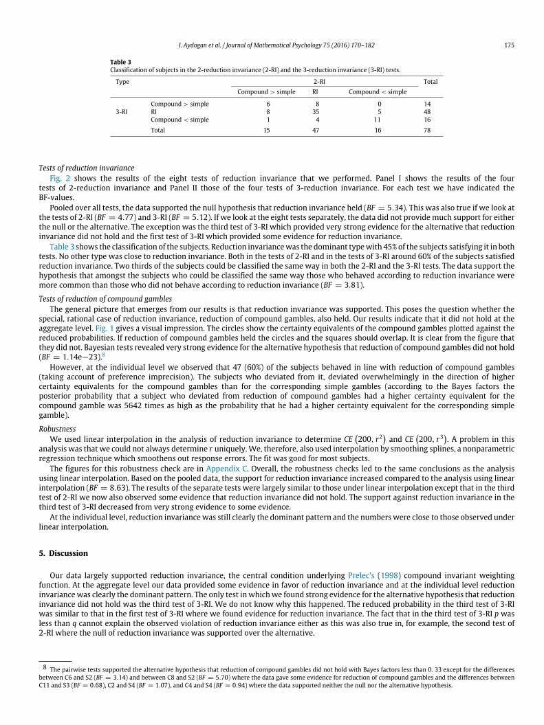
Table 3Classification of subjects in the 2-reduction invariance (2-RI) and the 3-reduction invariance (3-RI) tests.
Type 2-RI TotalCompound > simple RI Compound < simple
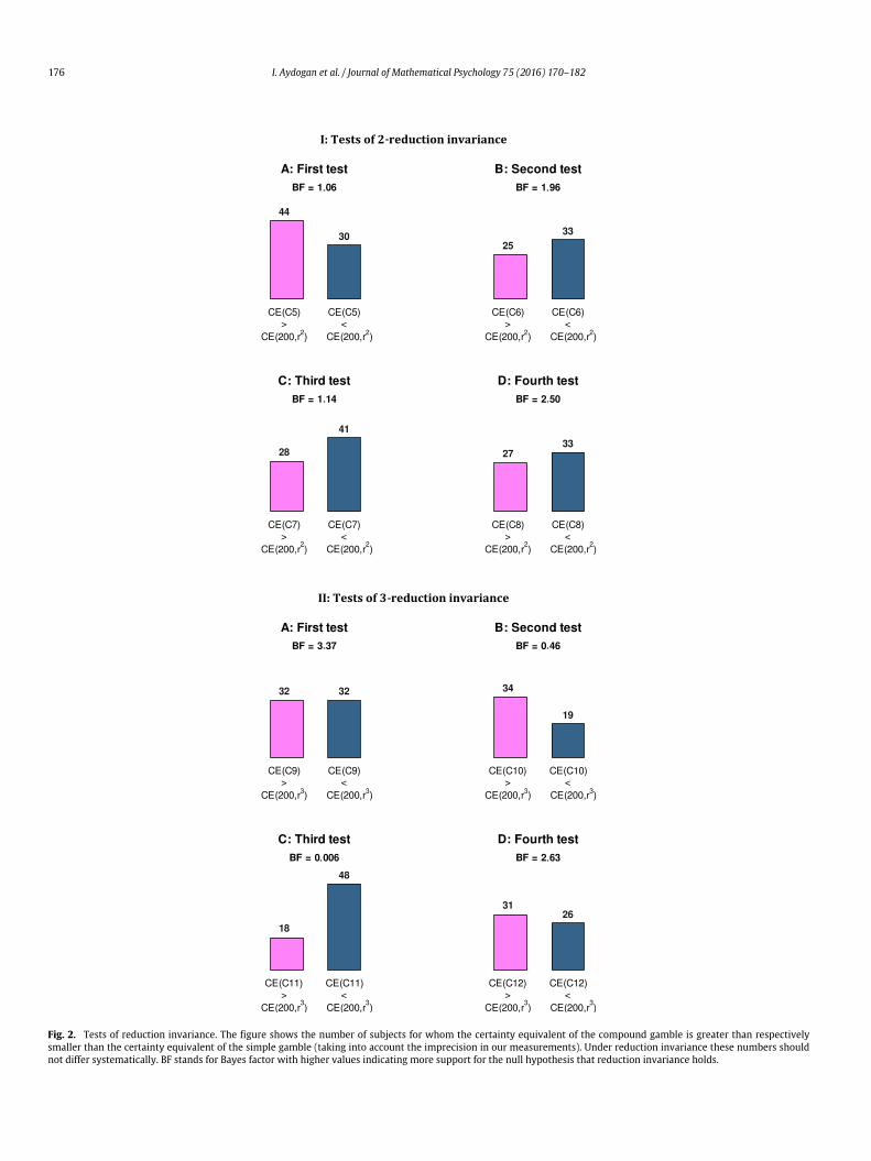
Tests of reduction invarianceFig. 2 shows the results of the eight tests of reduction invariance that we performed. Panel I shows the results of the four
tests of 2-reduction invariance and Panel II those of the four tests of 3-reduction invariance. For each test we have indicated theBF-values.
Pooled over all tests, the data supported the null hypothesis that reduction invariance held (BF = 5.34). This was also true if we look atthe tests of 2-RI (BF = 4.77) and 3-RI (BF = 5.12). If we look at the eight tests separately, the data did not providemuch support for eitherthe null or the alternative. The exception was the third test of 3-RI which provided very strong evidence for the alternative that reductioninvariance did not hold and the first test of 3-RI which provided some evidence for reduction invariance.
Table 3 shows the classification of the subjects. Reduction invariancewas the dominant typewith 45% of the subjects satisfying it in bothtests. No other type was close to reduction invariance. Both in the tests of 2-RI and in the tests of 3-RI around 60% of the subjects satisfiedreduction invariance. Two thirds of the subjects could be classified the same way in both the 2-RI and the 3-RI tests. The data support thehypothesis that amongst the subjects who could be classified the same way those who behaved according to reduction invariance weremore common than those who did not behave according to reduction invariance (BF = 3.81).
Tests of reduction of compound gamblesThe general picture that emerges from our results is that reduction invariance was supported. This poses the question whether the
special, rational case of reduction invariance, reduction of compound gambles, also held. Our results indicate that it did not hold at theaggregate level. Fig. 1 gives a visual impression. The circles show the certainty equivalents of the compound gambles plotted against thereduced probabilities. If reduction of compound gambles held the circles and the squares should overlap. It is clear from the figure thatthey did not. Bayesian tests revealed very strong evidence for the alternative hypothesis that reduction of compound gambles did not hold(BF = 1.14e−23).8
However, at the individual level we observed that 47 (60%) of the subjects behaved in line with reduction of compound gambles(taking account of preference imprecision). The subjects who deviated from it, deviated overwhelmingly in the direction of highercertainty equivalents for the compound gambles than for the corresponding simple gambles (according to the Bayes factors theposterior probability that a subject who deviated from reduction of compound gambles had a higher certainty equivalent for thecompound gamble was 5642 times as high as the probability that he had a higher certainty equivalent for the corresponding simplegamble).
RobustnessWe used linear interpolation in the analysis of reduction invariance to determine CE
200, r2
and CE
200, r3
. A problem in this
analysis was that we could not always determine r uniquely.We, therefore, also used interpolation by smoothing splines, a nonparametricregression technique which smoothens out response errors. The fit was good for most subjects.
The figures for this robustness check are in Appendix C. Overall, the robustness checks led to the same conclusions as the analysisusing linear interpolation. Based on the pooled data, the support for reduction invariance increased compared to the analysis using linearinterpolation (BF = 8.63). The results of the separate tests were largely similar to those under linear interpolation except that in the thirdtest of 2-RI we now also observed some evidence that reduction invariance did not hold. The support against reduction invariance in thethird test of 3-RI decreased from very strong evidence to some evidence.
At the individual level, reduction invariancewas still clearly the dominant pattern and the numbers were close to those observed underlinear interpolation.
5. Discussion
Our data largely supported reduction invariance, the central condition underlying Prelec’s (1998) compound invariant weightingfunction. At the aggregate level our data provided some evidence in favor of reduction invariance and at the individual level reductioninvariancewas clearly the dominant pattern. The only test inwhichwe found strong evidence for the alternative hypothesis that reductioninvariance did not hold was the third test of 3-RI. We do not know why this happened. The reduced probability in the third test of 3-RIwas similar to that in the first test of 3-RI where we found evidence for reduction invariance. The fact that in the third test of 3-RI p wasless than q cannot explain the observed violation of reduction invariance either as this was also true in, for example, the second test of2-RI where the null of reduction invariance was supported over the alternative.
8 The pairwise tests supported the alternative hypothesis that reduction of compound gambles did not hold with Bayes factors less than 0. 33 except for the differencesbetween C6 and S2 (BF = 3.14) and between C8 and S2 (BF = 5.70) where the data gave some evidence for reduction of compound gambles and the differences betweenC11 and S3 (BF = 0.68), C2 and S4 (BF = 1.07), and C4 and S4 (BF = 0.94) where the data supported neither the null nor the alternative hypothesis.
176 I. Aydogan et al. / Journal of Mathematical Psychology 75 (2016) 170–182
Fig. 2. Tests of reduction invariance. The figure shows the number of subjects for whom the certainty equivalent of the compound gamble is greater than respectivelysmaller than the certainty equivalent of the simple gamble (taking into account the imprecision in our measurements). Under reduction invariance these numbers shouldnot differ systematically. BF stands for Bayes factor with higher values indicating more support for the null hypothesis that reduction invariance holds.
I. Aydogan et al. / Journal of Mathematical Psychology 75 (2016) 170–182 177
Our tests of reduction invariance require the use of measured certainty equivalents. Luce (2000) argues that certainty equivalents maylead to biased estimations of the subjective values of gambles due to inherently different attitudes towards gambles (multi-dimensionalentities) and certain money amounts (one-dimensional entities). Von Nitzsch andWeber (1988) demonstrated empirical evidence of thisbias. This problem could be avoided by matching gambles with gambles, i.e. by directly elicitating r such that ((x, p), q) ∼ (x, r) and thenchecking whether ((x, pN), qN) ∼ (x, rN), N = 2, 3. As Luce (2001) pointed out, this test carries the risk that subjects will give the salientanswer pq = r in spite of the many observed empirical violations of reduction of compound gambles. We, therefore, followed Luce’s(2001) suggestion to use certainty equivalents in the tests of reduction invariance. To reduce possible distortions, we used a choice-basedprocedure to determine the certainty equivalents. Previous evidence suggests that observed anomalies are substantially reduced whenchoice-based certainty equivalents are used instead of judged certainty equivalents (Bostic et al., 1990; von Winterfeldt et al., 1997). Theprocedure we used is close to the PEST procedure used by Luce in his experimental research (Cho & Luce, 1995; Cho et al., 1994; Chunget al., 1994).
We used several ways to account for the stochastic nature of people’s preferences. Rather than testing equality of certainty equivalentswe followed Cho and Luce (1995) and tested whether the proportion of subjects for whom CE
200, pN
, qN
exceeded CE
200, rN
was the same as the proportion of subjects for whom CE
200, pN
, qN
was less than CE
200, rN
. Moreover, we accounted for the
imprecision in our measurements and in the individual analyses we only required preference patterns to hold in a majority of cases.There exist different and more sophisticated procedures to model choice errors. For example, Davis-Stober (2009) derived statistical testsbased on order-constrained inference techniques, which were applied, amongst others in Regenwetter, Dana, and Davis-Stober (2011) totest transitivity and in Davis-Stober, Brown, and Cavagnaro (2015) to compare models based on strict weak order representations withthose based on lexicographic semiorder representations. It is interesting to repeat our analysis using these methods, but it should berealized that they are, to the best of our knowledge, not yet applicable to matching tasks and that they require each choice to be repeatedmany times. In our experiment subjects made around 100 choices, but if we were to use the same amount of repetitions as Regenwetteret al. (2011) or Regenwetter and Davis-Stober (2012) did, subjects would have to make more than 2000 choices, which might reduceaccuracy.
We found mixed support for reduction of compound gambles, the rational special case of reduction invariance. The condition wasclearly violated at the aggregate level, but 60% of the subjects behaved in line with it. The violations of reduction of compound gamblesthat we observed indicate that subjects generally preferred compound gambles to simple gambles giving the same reduced probability.This compound risk seeking is consistent with Friedman (2005) and Kahn and Sarin (1988). It could be explained by a utility of gambling(Luce & Marley, 2000; Luce, Ng, Marley, & Aczél, 2008) as the compound gambles offer the possibility to gamble twice. On the otherhand, Abdellaoui et al. (2015) observed that their subjects were compound risk averse and preferred simple gambles with the samereduced probability. They also observed that subjects became more compound risk averse for higher probabilities, while we observedthe opposite pattern. The range of probabilities Abdellaoui et al. explored is larger than the range we explored. Moreover, the compoundgambles for which they found compound risk aversion weremore complex than the compound gambles we used and it wasmore difficultfor their subjects to compute the reduced probabilities. Complexity aversion may have contributed to compound risk aversion in theirstudy.
We obtained some evidence that when choosing between two gambles with the same expected value, subjects preferred the gamblewith the higher second-stage probability to the gamble with the higher first-stage probability. This is consistent with a preference tohave most uncertainty resolved at the first stage and violates event commutativity (Luce, 2000). We found very strong evidence thatthe certainty equivalent of C7, which offered a higher probability at the second stage, was higher than the certainty equivalent ofC4, which offered the approximately the same reduced probability but a higher first-stage probability (according to the Bayes factors,the posterior probability that CE(C7) > CE(C4) was 471 times as high as the probability that CE(C7) < CE(C4)). More support for apreference to have the high probability resolved later comes from a comparison of compound gambles C1 and C3, which were alsoclose in reduced probability. We found very strong evidence that the certainty equivalent of C3, which offered a larger second-stageprobability exceeded that of C1, which offered a larger first-stage probability (odds 56.93). On the other hand, we also found strongevidence that the certainty equivalent of gamble C5 exceeded the certainty equivalent of gamble C2 (odds 20.41), which is inconsistentwith a preference to have the high probability resolved later. As mentioned above, Budescu and Fischer (2001) and Ronen (1973)obtained clear evidence to have the high probability resolved first. Budescu and Fischer (2001) observed that hope was an importantreason why their subjects preferred higher initial probabilities. A typical reason subjects gave was that ‘‘the progress from one stageto the other means something, it’s better to lose at a later stage’’. Apparently, such considerations played no role in our study orthey were offset by other considerations such as disappointment aversion which predicts that the high probability will be resolvedlater.
6. Conclusion
Prelec’s (1998) compound-invariant family provides a simple way to model deviations from expected utility. It has a preferencefoundation, its parameters are intuitive, and it has often been used in empirical research. Luce (2001) gave an elegant simplificationof Prelec’s central condition and our study showed evidence in support of Luce’s central condition, reduction invariance. This impliesthat Prelec’s function provides an accurate description of the way people weight probabilities and endorses its use in empirical research.Reduction of compound gambles, a special case of reduction invariance, which is often considered rational, was rejected at the aggregatelevel, even though 60% of the subjects behaved in line with it implying that the power probability weighting function, which depends onreduction of compound gambles, should be used with caution.
Acknowledgments
We are grateful to the guest editor Clintin Davis-Stober, Vitalie Spinu, Peter P. Wakker, and two anonymous reviewers for theircomments on an earlier version of this paper.
178 I. Aydogan et al. / Journal of Mathematical Psychology 75 (2016) 170–182
Appendix A. Instructions and comprehension questions
I. Aydogan et al. / Journal of Mathematical Psychology 75 (2016) 170–182 179
180 I. Aydogan et al. / Journal of Mathematical Psychology 75 (2016) 170–182
Appendix B. The iteration procedure
Subjects always chose between a gamble and a sure amount x.
1. The initial value of xwas the even number closest to the expected value of the gamble.2. xwas decreased when it was chosen over the gamble and increased when the gamble was chosen.3. The initial step size was 4, 8, 16, or 32. By choosing powers of 2 we ensured that subsequent changes were also integers. The initial step
size was the number in the set {4, 8, 16, 32} that was closest to half the initial value.4. The step size remained constant until the subjects switched. Then it was halved.5. Theminimum step size was 2. The switching point was themidpoint between the largest value of x for which the gamble was preferred
and the smallest value of x for which xwas preferred.6. If a subject had to choose between 200 for sure and the gamble or between 0 for sure and the gamble and he chose the dominated
option, a warning message appeared: ‘‘Please reconsider your choice’’. The subject was asked to choose again. If the subject continuedto choose the dominated choice, we proceeded to the next elicitation.
Table B.1 shows the initial values and the initial step sizes for the eighteen gambles in the experiment.
Table B.1Initial values and initial step sizes for the gambles in the experiment.
Gamble Expected value Initial value Initial step size
Appendix C. Tests of reduction invariance under fitting of the certainty equivalents by smoothing splines
Figs. C.1 and C.2 and Table C.1 show the results when the weighting function is estimated by smoothing splines and this estimation isused to determine the certainty equivalents.
I. Aydogan et al. / Journal of Mathematical Psychology 75 (2016) 170–182 181
Fig. C.1. Tests of 2-reduction invariance.
Fig. C.2. Tests of 3-reduction invariance.
Table C.1Classification of subjects in the 2-reduction invariance (2-RI) and the 3-reduction invariance (3-RI) tests.
Type 2-RI TotalCompound > simple RI Compound < simple
182 I. Aydogan et al. / Journal of Mathematical Psychology 75 (2016) 170–182
References
Abdellaoui, M., Klibanoff, P., & Placido, L. (2015). Experiments on compound risk in relation to simple risk and to ambiguity.Management Science, 61, 1306–1322.Aczél, J., & Luce, R. D. (2007). A behavioral condition for Prelec’s weighting function on the positive line without assumingW (1) = 1. Journal of Mathematical Psychology, 51,
126–129.Bar-Hillel, M. (1973). On the subjective probability of compound events. Organizational Behavior and Human Performance, 9, 396–406.Bernasconi, M., & Loomes, G. (1992). Failures of the reduction principle in an Ellsberg-type problem. Theory and Decision, 32, 77–100.Bleichrodt, H., Kothiyal, A., Prelec, D., & Wakker, P. P. (2013). Compound invariance implies prospect theory for simple prospects. Journal of Mathematical Psychology, 57,
68–77.Bostic, R., Herrnstein, R. J., & Luce, R. D. (1990). The effect on the preference reversal of using choice indifferences. Journal of Economic Behavior and Organization, 13, 193–212.Budescu, D. V., & Fischer, I. (2001). The same but different: an empirical investigation of the reducibility principle. Journal of Behavioral Decision Making , 14, 187–206.Chechile, R. A., & Barch, D. H. (2013). Using logarithmic derivative functions for assessing the risky weighting function for binary gambles. Journal of Mathematical Psychology,
57, 15–28.Cho, Y., & Luce, R. D. (1995). Tests of hypotheses about certainty equivalents and joint receipt of gambles. Organizational Behavior and Human Decision Processes, 64, 229–248.Cho, Y., Luce, R. D., & Von Winterfeldt, D. (1994). Tests of assumptions about the joint receipt of gambles in rank-and sign-dependent utility theory. Journal of Experimental
Psychology: Human Perception and Performance, 20, 931–943.Chung, N. K., von Winterfeldt, D., & Luce, R. D. (1994). An experimental test of event commutativity in decision making under uncertainty. Psychological Science, 5, 394–400.Currim, I. S., & Sarin, R. K. (1989). Prospect versus utility.Management Science, 35, 22–41.Davis-Stober, C. P. (2009). Analysis ofmultinomialmodels under inequality constraints: applications tomeasurement theory. Journal of Mathematical Psychology, 53(1), 1–13.Davis-Stober, C. P., Brown, N., & Cavagnaro, D. R. (2015). Individual differences in the algebraic structure of preferences. Journal of Mathematical Psychology, 66, 70–82.Diecidue, E., Schmidt, U., & Zank, H. (2009). Parametric weighting functions. Journal of Economic Theory, 144, 1102–1118.Fox, C. R., & Poldrack, R. A. (2014). Prospect theory and the brain. In Paul Glimcher, & Ernst Fehr (Eds.), Handbook of neuroeconomics (2nd ed.) (pp. 533–567). New York:
Elsevier.Friedman, Z. G. (2005). Evaluating risk in sequential events: violations in expected utility theory.Washington University Undergraduate Research Digest , 1, 29–39.Goldstein, W. M., & Einhorn, H. J. (1987). Expression theory and the preference reversal phenomena. Psychological Review, 94, 236–254.Gonzalez, R., & Wu, G. (1999). On the form of the probability weighting function. Cognitive Psychology, 38, 129–166.Gul, F. (1991). A theory of disappointment aversion. Econometrica, 59, 667–686.Hastie, T., Tibshirani, R., & Friedman, J. (2008). The elements of statistical learning: data mining, inference and prediction (2nd ed.). Berlin: Springer.Jeffreys, H. (1961). Theory of probability (3rd ed.). New York: Oxford University Press.Kahn, B. E., & Sarin, R. K. (1988). Modeling ambiguity in decisions under uncertainty. Journal of Consumer Research, 15, 265–272.Karmarkar, U. A. (1978). Subjectively weighted utility: a descriptive extension of the expected utility model. Organizational Behavior and Human Performance, 21, 61–72.Keller, L. R. (1985). Testing of the ‘reduction of compound alternatives’ principle. Omega, 13, 349–358.Lattimore, P. M., Baker, J. R., & Witte, A. D. (1992). The influence of probability on risky choice. Journal of Economic Behavior and Organization, 17, 377–400.Luce, R. D. (1990). Rational versus plausible accounting equivalences in preference judgments. Psychological Science, 1, 225–234.Luce, R. D. (1991). Rank- and sign-dependent linear utility models for binary gambles. Journal of Economic Theory, 53, 75–100.Luce, R. D. (1996). When four distinct ways to measure utility are the same. Journal of Mathematical Psychology, 40, 297–317.Luce, R. D. (2000). Utility of gains and losses: measurement-theoretical and experimental approaches. Mahwah, New Jersey: Lawrence Erlbaum Associates, Inc..Luce, R. D. (2001). Reduction invariance and Prelec’s weighting functions. Journal of Mathematical Psychology, 45, 167–179.Luce, R. D. (2002). A psychophysical theory of intensity proportions, joint presentations, and matches. Psychological Review, 109, 520.Luce, R. D. (2004). Symmetric and asymmetric matching of joint presentations. Psychological Review, 111, 446.Luce, R. D., & Fishburn, P. C. (1991). Rank- and sign-dependent linear utility models for finite first-order gambles. Journal of Risk and Uncertainty, 4, 29–59.Luce, R. D., & Fishburn, P. C. (1995). A note on deriving rank-dependent utility using additive joint receipts. Journal of Risk and Uncertainty, 11, 5–16.Luce, R. D., & Marley, A. A. (2000). On elements of chance. Theory and Decision, 49, 97–126.Luce, R. D., Ng, C., Marley, A., & Aczél, J. (2008). Utility of gambling II: risk, paradoxes, and data. Economic Theory, 36, 165–187.Marley, A., & Luce, R. D. (2002). A simple axiomatization of binary rank-dependent utility of gains (losses). Journal of Mathematical Psychology, 46, 40–55.Morey, R. D., Rouder, J. N., Jamil, T., & R Core Team, (2015). BayesFactor. Vienna, Austria: R Foundation for Statistical Computing.Prelec, D. (1998). The probability weighting function. Econometrica, 66, 497–528.Quiggin, J. (1981). Risk perception and risk aversion among Australian farmers. Australian Journal of Agricultural Economics, 25, 160–169.Quiggin, J. (1982). A theory of anticipated utility. Journal of Economic Behavior and Organization, 3, 323–343.R Core Team (2015). R: a language and environment for statistical computing. Vienna, Austria: R Foundation for Statistical Computing.Regenwetter, M., Dana, J., & Davis-Stober, C. P. (2011). Transitivity of preferences. Psychological Review, 118, 42–56.Regenwetter, M., & Davis-Stober, C. P. (2012). Behavioral variability of choices versus structural inconsistency of preferences. Psychological Review, 119, 408.Ronen, J. (1973). Effects of some probability displays on choices. Organizational Behavior and Human Performance, 9, 1–15.Rouder, J. N., Morey, R. D., Speckman, P. L., & Province, J. M. (2012). Default Bayes factors for ANOVA designs. Journal of Mathematical Psychology, 56, 356–374.Rouder, J. N., Speckman, P. L., Sun, D., Morey, R. D., & Iverson, G. (2009). Bayesian t tests for accepting and rejecting the null hypothesis. Psychonomic Bulletin & Review, 16,
225–237.Slovic, P. (1969). Manipulating the attractiveness of a gamble without changing its expected value. Journal of Experimental Psychology, 79, 139.Sneddon, R., & Luce, R. D. (2001). Empirical comparisons of bilinear and nonbilinear utility theories. Organizational Behavior and Human Decision Processes, 84, 71–94.Stott, H. P. (2006). Cumulative prospect theory’s functional menagerie. Journal of Risk and Uncertainty, 32, 101–130.Tversky, A., & Kahneman, D. (1992). Advances in prospect theory: cumulative representation of uncertainty. Journal of Risk and Uncertainty, 5, 297–323.Von Nitzsch, R., & Weber, M. (1988). Utility function assessment on a micro-computer: an interactive procedure. Annals of Operations Research, 16, 149–160.von Winterfeldt, D., Chung, N., Luce, R. D., & Cho, Y. (1997). Tests of consequence monotonicity in decision making under uncertainty. Journal of Experimental Psychology:
Learning, Memory, and Cognition, 23, 406–426.Wakker, P. P. (2010). Prospect theory: for risk and ambiguity. Cambridge UK: Cambridge University Press.Wakker, P. P., Erev, I., & Weber, E. U. (1994). Comonotonic independence: the critical test between classical and rank-dependent utility theories. J. Risk and Uncertain., 9,