An Experimental Test of the Anscombe-Aumann Monotonicity Axiom · Working Paper No. 207 An...

Working Paper No. 207

An Experimental Test of the Anscombe-Aumann Monotonicity Axiom

Florian Schneider and Martin Schonger

Revised version, May 2017

University of Zurich

Department of Economics

Working Paper Series

ISSN 1664-7041 (print) ISSN 1664-705X (online)

AN EXPERIMENTAL TEST OF THE ANSCOMBE-AUMANNMONOTONICITY AXIOM

FLORIAN H. SCHNEIDER AND MARTIN SCHONGER

Abstract. Most models of ambiguity aversion satisfy Anscombe-Aumann’s Monotonicity axiom.

Monotonicity imposes separability of preferences across events that occur with unknown probabil-

ity. We construct a test of Monotonicity by modifying the Allais paradox to a setting with both

subjective and objective uncertainty. Two experimental studies are conducted: while study 1 uses

U.S. online workers and a natural source of ambiguity, study 2 employs European students and

an Ellsberg urn. In both studies, modal behavior violates Monotonicity in a specific, intuitive

way. Overall, our data suggest that violations of Monotonicity are as prevalent as violations of von

Neumann-Morgenstern’s Independence axiom.

1. Introduction

Since Ellsberg (1961) pioneered the concept of ambiguity aversion, both theorists and experi-

menters have taken a keen interest in the concept. Ambiguity aversion is usually studied in the

Anscombe-Aumann (1963) framework. Anscombe-Aumann proposed a monotonicity axiom. Their

Monotonicity axiom prescribes that if two acts differ only on a single state, then the preference

between these two acts is given by the preference between the lotteries that are assigned to that

state. While both this description of the axiom and its name suggest that it is a mere dominance

axiom, Monotonicity is a separability axiom like von Neumann-Morgenstern’s Independence ax-

iom. Although Monotonicity is assumed in the majority of models of ambiguity aversion and is

controversial, it has not been tested so far. This paper provides an experimental approach to test

Monotonicity and then employs it.

Apart from basic choice theoretic axioms like transitivity and continuity, Monotonicity seems to be

the most common axiom employed in models of ambiguity aversion. Within the Anscombe-Aumann

Schneider: Department of Economics, University of Zurich, [email protected]. Schonger: Center forLaw and Economics, ETH Zurich, [email protected] helpful discussions we would like to thank Björn Bartling, Michael H. Birnbaum, Marie-Charlotte Gütlein, AndreasHaller, Glenn Harrison, Damian Kozbur, Felix Kübler, Jörg Oechssler, Ivo Schurtenberger, Stefan Trautmann, PeterWakker, Roberto A. Weber, and seminar participants at the European Economic Association, Nordic Conference onBehavioral and Experimental Economics, Conférence Universitaire de Suisse Occidentale, Foundations of Utility andRisk, Royal Economic Society, Berlin Behavioral Economics Seminar, Schweizerische Gesellschaft für Volkswirtschaftund Politik, Toulouse School of Economics, Universities of Tübingen and Heidelberg, and ETH Zurich. GabrielGertsch, Sean Hofland and Himanshu Jain provided excellent research assistance. Financial support from the Chairof Gérard Hertig is gratefully acknowledged.A previous version of this paper was titled “Allais at the Horse Race: Testing Models of Ambiguity Aversion.”

1

mailto:[email protected]

mailto:[email protected]

SCHNEIDER/SCHONGER 2

framework, models of ambiguity aversion that satisfy Monotonicity include Multiple priors (Gilboa

and Schmeidler, 1989), the Rank-Dependent/Choquet Model (Schmeidler, 1989), Smooth ambiguity

preferences (Klibanoff, Marinacci, and Mukerji, 2005), Variational preferences (Maccheroni, Mari-

nacci, and Rustichini, 2006), Confidence-function preferences (Chateauneuf and Faro, 2009), Vector

Expected Utility (Siniscalchi, 2009), Uncertainty-averse preferences (Cerreia-Vioglio, Maccheroni,

Marinacci, and Montrucchio, 2011), MBA-preferences (Cerreia-Vioglio, Ghirardato, Maccheroni,

Marinacci, and Siniscalchi, 2011), monotone Mean-dispersion preferences (Grant and Polak, 2013),

and Hedging preferences (Dean and Ortoleva, forthcoming). There are far fewer models that do not

impose Monotonicity; they include non-monotone Mean-dispersion preferences (Grant and Polak,

2013), and Bommier’s (2016) dual approach.

Monotonicity is a controversial axiom: Some see it as one of the “basic tenets of rationality under

ambiguity” (Cerreia-Vioglio, Ghirardato, Maccheroni, Marinacci, and Siniscalchi, 2011), or “a basic

rationality axiom” (Gilboa and Marinacci, 2013). Skiadas (2013) assumes Monotonicity, but calls

it “not an innocuous assumption”. Others view Monotonicity as untenable for non-expected utility

decision-makers: Non-expected utility implies that preferences are not separable across events that

occur with known probability, yet Monotonicity implies that preferences are separable across events

that occur with unknown probability. Wakker (2010 p.301f.; 2011) argues that under non-expected

utility, separability across ambiguous events is “undesirable”, “implausible”, and “unreasonable”.

Machina (2009) takes the view that “the phenomenon of ambiguity aversion is intrinsically one of

nonseparable preferences across mutually exclusive events.”

This paper proposes a thought experiment that directly tests Monotonicity. The thought experi-

ment is an adaptation of the classic Allais paradox. Recall that the Allais paradox is set in a world of

purely objective uncertainty, and tests expected utility, specifically the von Neumann-Morgenstern

Independence axiom. Previous authors (MacCrimmon and Larsson, 1979; Tversky and Kahneman,

1992; Wu and Gonzalez, 1999) have adapted the Allais paradox to a setting of purely subjective

uncertainty, where it becomes a test of Subjective Expected Utility. We adapt the Allais paradox

to a setting of both objective and subjective uncertainty. The so-modified Allais paradox tests

Monotonicity. As sources of objective and subjective uncertainty the thought experiment employs

the Anscombe-Aumann metaphors of a horse race and a roulette wheel, respectively. The payoff

of the decision-maker depends on the outcome of both sources of uncertainty (see figure 1). The

thought experiment, like the Allais paradox, has large hypothetical payoffs. It can be implemented

as an incentivized experiment by scaling down the payoffs, and employing practical sources of un-

certainty such as Ellsberg urns. Building a test of the descriptive validity of Monotonicity on the


Allais paradox is advantageous: The extensive literature on the Allais paradox can inform the scal-

ing of the payoffs, and can serve to benchmark the rate of violations. The Allais literature also

suggests potential causes of violations, e.g. the certainty effect. While the main purpose of the

thought experiment is to suggest incentivized tests, it is also useful in its hypothetical form: Some

have understood the Allais paradox as a critique of the view that Independence is a prerequisite of

rationality (e.g. Slovic and Tversky, 1974; Allais, 1979 chapter II 3.4; Loomes and Sugden, 1982;

Machina, 1989). Similarly, our thought experiment facilitates discussions of whether Monotonicity

is a prerequisite of rationality.

There is an extensive experimental literature on ambiguity attitudes, for recent reviews see Hey

(2014) and Trautmann and van de Kuilen (2015). However, we know of no experiments testing

the Monotonicity axiom. As for thought experiments, most closely related to ours are a few recent

thought experiments on separability across ambiguous events: Five thought experiments by Machina

(2014) demonstrate that separability restricts variation in ambiguity attitudes at low versus high

outcomes. Wakker (2010, p.302) employs a thought experiment in order to argue that separability

is implausible for ambiguity averse decision-makers. Bommier (2016) suggests another thought

experiment making this point. All these thought experiments are critiques of separability, but

none of them directly tests Monotonicity. As a practical matter, these thought experiments are

difficult to implement since they require exact measurement of certainty equivalents or a method

for implementing payoffs in utils.

We conduct two incentivized studies implementing our thought experiment. Study 1 uses a

subject pool of online workers, a real-world lottery as the source of objective uncertainty, and

weather in a foreign city for subjective uncertainty. Study 2 takes place in the laboratory with

student subjects and employs physical urns. Both studies find that about half of all participants

violate Monotonicity, and overwhelmingly do so in a specific, intuitive way. The hypothesis that

these violations are due to random errors is easily and robustly rejected in both studies. The

specific pattern of violations we find mirrors the pattern that is commonly found in Allais paradox

experiments. To be able to assess and interpret the frequency of violations of Monotonicity, it is

useful to compare it to the frequency of violations of Independence in the same subject pools. Hence

both studies also confront subjects with the original Allais paradox. Violations of Independence

are about as common as violations of Monotonicity in both studies. In addition, violations of

Independence and Monotonicity are positively correlated. Study 2 also includes a consistency check

by repeatedly posing the Monotonicity test. We find that among consistent participants violations

of Monotonicity are more prevalent than in the full sample. Overall, we conclude that violations


1A : $1 Million with certainty.

1B :

$0 Horse 1-11 wins and roulette stops on 1.$1 Million Horse 12-100 wins.$5 Million Horse 1-11 wins and roulette stops on 2-11.

2A :

{$0 Horse 12-100 wins.$1 Million Horse 1-11 wins.

2B :

$0 Horse 1-11 wins and roulette stops on 1,

or Horse 12-100 wins.$5 Million Horse 1-11 wins and roulette stops on 2-11.

Figure 1. Thought experiment

of Monotonicity are common and genuine. Knowledge of this phenomenon is important when

developing and evaluating descriptive models of ambiguity non-neutrality, as our findings suggest

that universally assuming Monotonicity is problematic.

The next section introduces our thought experiment. Section 3 reviews the Monotonicity axiom.

Section 4 describes the experimental studies. Section 5 concludes.

2. A thought Experiment

Our thought experiment uses the classic Anscombe-Aumann story of a horse race and a roulette

wheel. 100 horses numbered from 1 to 100 are starting. The decision-maker does not know the

probability that a particular horse will win. At the same time as the horses are running, the roulette

wheel is spun. The roulette wheel has 11 equiprobable fields numbered from 1 to 11. As shown

in figure 1, the decision-maker is confronted with two choice situations, 1 and 2. In each choice

situation she has the choice between two options, A and B. In choice situation 1 an intuitively

plausible choice, in line with the certainty effect, might be to choose 1A, which is a million for sure,

over 1B, where there is a chance of not winning anything. By contrast in choice situation 2 both

bets feature a danger of winning nothing, thus the chance of winning $5 Million in bet 2B may make

that bet more attractive than bet 2A. Observation 1 in the next section clarifies that this intuitive

choice pattern violates Monotonicity. From now on we refer to this choice pattern as the intuitive

paradoxical choice pattern.

Compare the thought experiment to the Allais paradox (Allais, 1953), reproduced in figure 2. Re-

call that in the Allais paradox all uncertainty is objective. Thus in the metaphors of the Anscombe-

Aumann framework, the Allais paradox only features a roulette wheel (albeit with more fields), but


IA : $1 Million with certainty.

IB :

$0 Roulette stops on 1.$1 Million Roulette stops on 2-90.$5 Million Roulette stops on 91-100.

IIA :

{$0 Roulette stops on 1-89.$1 Million Roulette stops on 90-100.

IIB :

{$0 Roulette stops on 1-90.$5 Million Roulette stops on 91-100.

Figure 2. Allais paradox

no horse race. Our thought experiment differs from the Allais paradox only in that it assigns some

uncertainty to a subjective source. Therefore, a decision-maker who does not distinguish between

objective and subjective uncertainty, i.e. a probabilistically sophisticated one, views our thought

experiment as an Allais paradox. If the decision-maker moreover assigns equal probabilities to the

horses, then she views our thought experiment as the same choice situation as the Allais paradox in

figure 2 (for a formal statement see p. 8). If she assigns non-equal probabilities, then the thought

experiment corresponds to an Allais paradox with probabilities possibly different from the ones in

figure 2.1

Again, let us call the pattern of choosing IA over IB and IIB over IIA the intuitive paradoxical choice

pattern, as it is analogous to the intuitive paradoxical choice pattern in our thought experiment.

The intuitive paradoxical choice pattern is what has often been found in experimental investigations

of the Allais paradox2, and constitutes a violation of Independence. Monotonicity is discussed in

the next section, and we show that it is tested by the modified Allais paradox.

3. The Anscombe-Aumann Monotonicity Axiom

To discuss Monotonicity and its implications, we introduce an Anscombe-Aumann framework:

There are (monetary) prizes x in an interval X = [x, x] ⊂ R. We denote the space of simple

probability distributions (lotteries) over X by L (X), with generic elements P,Q,R. Denote the

degenerate lottery which puts probability 1 on the prize x by δx. There is a (finite or infinite) set of

states S with generic element s, endowed with an algebra Σ (events). An act f is a Σ-measurable

1Except if she assigns probabilities such that the event “horse 1-11 wins” has probability 0 or 1, then the situationsbecome trivial.2See for example Kahneman and Tversky (1979), Conlisk (1989), and Huck and Müller (2012).


function3 f : S → L (X) such that f (S) = {f (s) : s ∈ S} is finite. The set of all acts is denoted

by F . Generic acts are f, g, h. For all acts f , g in F and all α in (0, 1) let αf + (1− α) g denote

the act that delivers the lottery αf (s) + (1− α) g (s) in state s. For every act f , we denote the

coarsest partition of the state space it induces by E(f) ={E ∈ Σ|E = f−1(P ) for some P ∈ f(S)

}.

Note that E(f) is finite. Given an event E ∈ Σ, acts f and g, let fEg denote the act which gives

f (s) for s ∈ E, and g (s) for s ∈ EC . An act that yields the same lottery P in each state is called

constant, and, slightly abusing notation, is denoted by P . Throughout we assume that objective

and subjective uncertainty are resolved simultaneously. % is a preference order on F :

Axiom (Weak order). % is complete and transitive.

Anscombe-Aumann (1963) proposed a monotonicity axiom which requires that if the lottery

which an act assigns to an event is replaced by a preferred lottery, then the new act must be

preferred. The modern literature formulates the Anscombe-Aumann Monotonicity axiom as follows

(under Weak order the modern and original formulations are equivalent):

Axiom (Monotonicity). For all acts f ,g in F : if for all states s in S, f (s) % g (s), then f % g.

Monotonicity implies that preferences are separable across events. Specifically, Monotonicity

implies that for all lotteries P,Q, all acts f, g, and all events E, if PEf � QEf then PEg % QEg.4

If the preference admits a utility representation, Monotonicity essentially ensures that one can

find a separable, weakly monotone representation. That is an act can be evaluated by a two-

step procedure: There is a preference functional and a real-valued, non-decreasing function. The

preference functional could, for example, be expected utility or rank-dependent expected utility

(Quiggin, 1982). For each state, the preference functional evaluates the lottery the act yields in

that state, independently of what the act yields in other states. For the case of a finite state space,

this yields |S| numbers which are then aggregated by the non decreasing function to a single number

representing the utility of the act (see Bommier, 2016, also Trautmann and Wakker, 2015).

Monotonicity is distinct from first-order stochastic dominance. A lottery P first-order stochasti-

cally dominates a lottery Q, if for all x′ we have∑

x:x≤x′ P (x) ≤∑

x:x≤x′ Q (x). For the Anscombe-

Aumann setting, Machina and Schmeidler (1995) propose a first-order stochastic dominance axiom:

Axiom (AA-FOSD). For all acts f ,g in F : if for all states s in S, f (s) first-order stochastically

dominates g (s), then f % g.

3In this definition, L (X) is endowed with any σ-algebra which makes singletons measurable.4A stronger version of separability, “PEf % QEf ⇒ PEg % QEg “, implies a slightly stronger version of Monotonicity,which is not satisfied by the Multiple priors model (Gilboa and Schmeidler, 1989).


When restricting the domain of AA-FOSD to constant acts, the standard first-order stochastic

dominance axiom (FOSD) results. Monotonicity is structurally similar to AA-FOSD and basically

stronger: as long as the decision-maker satisfies FOSD, Monotonicity implies AA-FOSD.

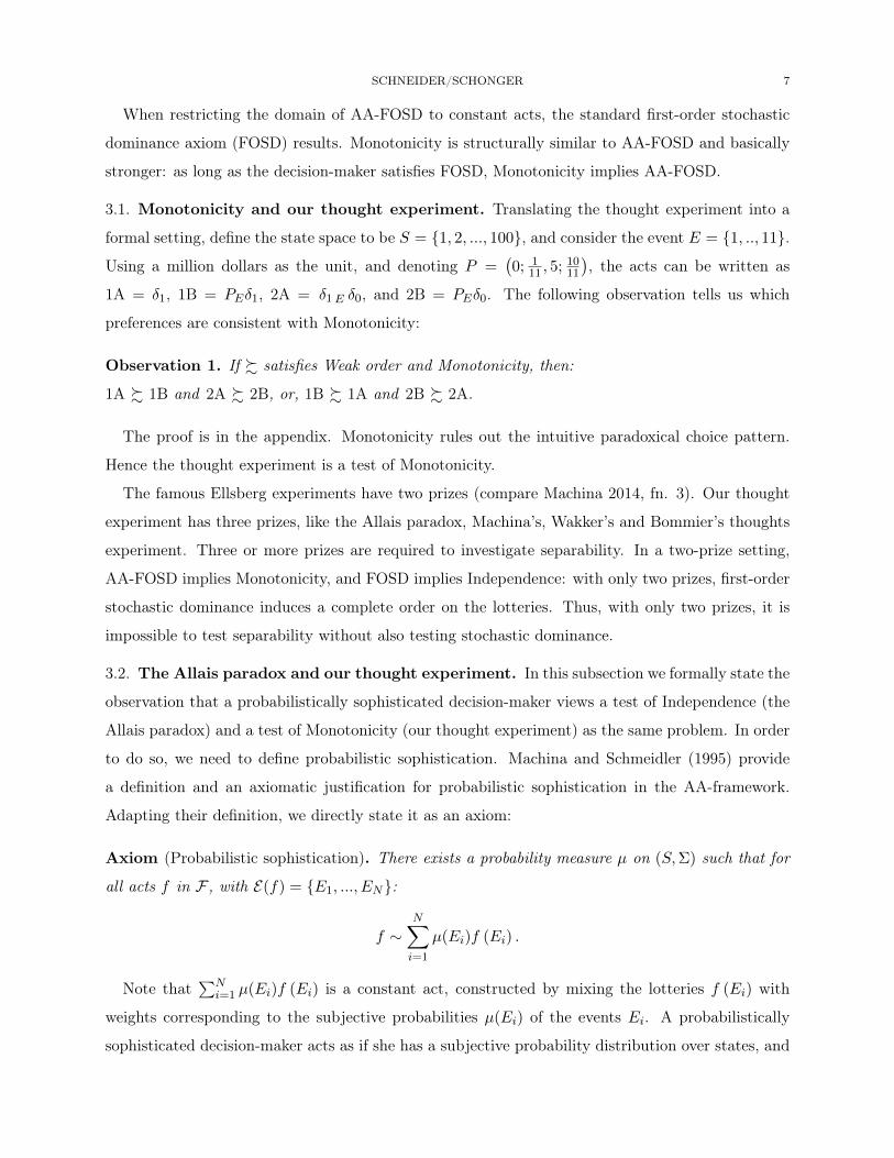
3.1. Monotonicity and our thought experiment. Translating the thought experiment into a

formal setting, define the state space to be S = {1, 2, ..., 100}, and consider the event E = {1, .., 11}.

Using a million dollars as the unit, and denoting P =(0; 1

11 , 5; 1011

), the acts can be written as

1A = δ1, 1B = PEδ1, 2A = δ1E δ0, and 2B = PEδ0. The following observation tells us which

preferences are consistent with Monotonicity:

Observation 1. If % satisfies Weak order and Monotonicity, then:

1A % 1B and 2A % 2B, or, 1B % 1A and 2B % 2A.

The proof is in the appendix. Monotonicity rules out the intuitive paradoxical choice pattern.

Hence the thought experiment is a test of Monotonicity.

The famous Ellsberg experiments have two prizes (compare Machina 2014, fn. 3). Our thought

experiment has three prizes, like the Allais paradox, Machina’s, Wakker’s and Bommier’s thoughts

experiment. Three or more prizes are required to investigate separability. In a two-prize setting,

AA-FOSD implies Monotonicity, and FOSD implies Independence: with only two prizes, first-order

stochastic dominance induces a complete order on the lotteries. Thus, with only two prizes, it is

impossible to test separability without also testing stochastic dominance.

3.2. The Allais paradox and our thought experiment. In this subsection we formally state the

observation that a probabilistically sophisticated decision-maker views a test of Independence (the

Allais paradox) and a test of Monotonicity (our thought experiment) as the same problem. In order

to do so, we need to define probabilistic sophistication. Machina and Schmeidler (1995) provide

a definition and an axiomatic justification for probabilistic sophistication in the AA-framework.

Adapting their definition, we directly state it as an axiom:

Axiom (Probabilistic sophistication). There exists a probability measure µ on (S,Σ) such that for

all acts f in F , with E(f) = {E1, ..., EN}:

f ∼N∑i=1

µ(Ei)f (Ei) .

Note that∑N

i=1 µ(Ei)f (Ei) is a constant act, constructed by mixing the lotteries f (Ei) with

weights corresponding to the subjective probabilities µ(Ei) of the events Ei. A probabilistically

sophisticated decision-maker acts as if she has a subjective probability distribution over states, and


she treats objective and subjective probabilities interchangeably. We can now state formally how,

given Probabilistic sophistication and informational symmetry, the Allais paradox and our thought

experiment are basically the same problem. Probabilistic sophistication means that the decision-

maker has a probability measure µ. Informational symmetry of the horses implies that µ (E) = 11100 .

By Probabilistic sophistication the decision-maker is indifferent between each act in the thought

experiment and the corresponding act in the Allais paradox: 1A ∼ IA, 1B ∼ IB, 2A ∼ IIA, and

2B ∼ IIB.

This observation motivates proposition 1. The purpose of proposition 1 is to illuminate that a

probabilistically sophisticated decision-maker views not only these tests as the same problem, but

views the axioms these experiments test as similar. Consider the Independence axiom for objective

risk, but restrict mixtures to a set M ⊆ (0, 1):

Axiom (Independence over M). For all constant acts P,Q,R, and for all α in M ⊆ (0, 1):

P % Q⇒ αP + (1− α)R % αQ+ (1− α)R.

Under probabilistic sophistication, Monotonicity is equivalent to Independence over Mµ, with

Mµ constructed from µ:

Proposition 1. If % satisfies Weak order and Probabilistic sophistication with probability measure

µ, then Monotonicity and Independence over

Mµ = {m ∈ (0, 1) |m = µ(E) for some E ∈ Σ} are equivalent.

The proof is in the appendix. Thus (unrestricted) Independence implies Monotonicity. If Mµ

is the unit interval, then the converse is true. For Mµ to be the unit interval requires an infinite

state space, and a non-atomicity assumption on µ. Note that in the Anscombe-Aumann frame-

work, Independence is usually strengthened to the AA-Independence axiom. Under probabilistic

sophistication, however, Independence implies AA-Independence (see lemma 1, p. 23).

3.3. Critiques of separability. In a setting of purely objective uncertainty, separability is cap-

tured by the Independence axiom. Independence is often understood as a prerequisite for rationality,

but at least since the Allais paradox this has been doubted. Machina (1989) challenges Indepen-

dence on normative grounds, pointing out that the description of consequences available to the

economist might not be deep enough for separability to hold, say, because it leaves out psycholog-

ical components such as disappointment, and that therefore in such contexts Independence may

be normatively inappropriate. Loomes and Sugden (1982) argue that regret and rejoicing are ex-

periences, and thus cannot be rational or irrational. Accordingly, they take the position that if a


decision-maker experiences such feelings, taking them into account for decision-making should not

be seen as irrational. For a detailed critique of this argument see Bleichrodt and Wakker (2015).

Our thought experiment shows that such critiques of separability as prerequisite for rationality

in a setting of purely objective uncertainty also apply in a setting of mixed subjective/objective

uncertainty. In this sense, the thought experiment contributes to discussing Monotonicity from a

normative perspective.

Under ambiguity, separability has another, potentially undesirable, implication, namely it rules

out some forms of ambiguity aversion: Take two lotteries P and Q with P 6= Q and P ∼ Q, and a

partition of the state space into two non-null events, E and its complement. Consider the act f =

PEQ. Note that the act f is an ambiguous act, while the constant act P has no ambiguity. Thus one

might expect an ambiguity-averse decision-maker to strictly prefer P over f . Monotonicity, however,

requires the decision-maker to be indifferent. The logic of this example follows Wakker (2010,

p. 302). Machina (2014) provides five thought experiments, which demonstrate that separability

restricts how ambiguity aversion can differ between high and low outcomes.

4. Experiments

To find out to what extent the Monotonicity axiom is descriptively valid, and to compare and

relate the prevalence of potential violations of Monotonicity to those of Independence, we run two

experimental studies. Study 1 is conducted with a subject pool of online workers and employs a

natural source of ambiguity, whereas study 2 is run in the lab with undergraduate student subjects

and employs physical urns.

4.1. Study 1 (Online Experiment).

4.1.1. Procedure. To implement the thought experiment as an experimental test of Monotonicity,

we adapt the prizes and the sources of uncertainty as follows: For the non-zero prizes, rather than $1

Million and $5 Million we use $4 and $5. Instead of a horse race, the source of subjective uncertainty

is weather in a foreign city as in Fox and Tversky (1995). Specifically, for the event E take the

event that tomorrow’s maximum temperature in Mexico City is “unexpectedly high”. We define

“unexpectedly high” as 6° Fahrenheit (3.3° Celsius) or more above the current forecast. Participants

are told the current forecast and are encouraged to check it on an external website, which shows

forecasts and past realizations rounded to integer degrees Fahrenheit. For objective uncertainty we

use “Texas Pick 3”, a real-world U.S. lottery, which produces the numbers between 000 and 999 with

equal probability. In the test of Monotonicity we consider the last digit, in the Allais paradox the

last two digits. So we slightly modify the objective probabilities from our thought experiment (10


instead of 11 equiprobable objective events). With these modifications, denoting Q =(0; 1

10 , 5; 910

),

we get the experimental acts 1A= δ4, 1B = QEδ4, 2A = δ4E δ0, and 2B = QEδ0. Figure 3 shows,

using the example of act 1B, how acts are displayed to participants (the temperature symbols are

defined and explained to participants). Note that observation 1 analogously applies to the acts

in the experiment. For the Allais paradox, the lotteries in the experiment differ from the original

lotteries only in the prizes as described above.

Figure 3. Visual representation of act 1B

Participants were recruited on Amazon Mechanical Turk (mTurk). We restricted participation

to U.S. workers. All subjects completed the study within a few hours on the same day. Average

earnings were $0.70 (EC realized), average duration was 10 minutes, implying an hourly wage of

$4.20.

The sequence of the experiment is as follows: the format of the acts is explained, including links to

the external weather forecast website and the Texas Pick 3 website, followed by three understanding

questions. As a further test of participants’ understanding, the subsequent screen offers a choice

between two acts, where one act dominates the other in the AA-FOSD sense. On this screen, as

well as the Monotonicity and Allais paradox screens, subjects are given a choice between two acts,

which are presented in random order. The next two screens each present a choice situation of the

Monotonicity test, where the order of the screens (choice situations) is random. This is followed

by the two Allais paradox choice situations, which are again displayed in random order. We also

measured participants’ beliefs about the probability of the events. We use the Random Lottery

Incentive (RLI) system to make hedging impossible. A demographic survey concludes the study.5

4.1.2. Results. Data from N = 552 participants was collected. Table 1i gives participants’ choices

in the Monotonicity test. Consider the first row of results, which concerns the full sample. Choices

in columns AA and BB do not violate Monotonicity, choices in columns AB and BA do. The

modal choice of participants violates Monotonicity in a particular way: 38.8 percent of participants

exhibit the intuitive paradoxical choice pattern AB. Violations of Monotonicity are not random,

5The web appendix supplies screenshots and a detailed description of the experiment.


rather, there is an asymmetric pattern, as violations in the opposite way are much rarer with

9.2 percent. Following Conlisk (1989), we test whether violations are the result of symmetric,

random participant error. We can reject this hypothesis at all conventional significance levels

(Z = 11.06, p-value < 10−28). The following rows repeat the analysis for different subsamples as

robustness checks. The second row considers only participants who do not violate AA-FOSD. The

next four rows split the sample by duration. The picture which emerges is that the distribution

of violations is very similar across subsamples. Table 5i (appendix, p.25) finds robustness across

further subsamples.

Table 1. Violations of Monotonicity and Independence (in percent)

Satisfy Violate

AA BB AB BA Conl.-Z N

(i) MonotonicityFull sample 36.8 15.2 38.8 9.2 11.06 552Satisfy AA-FOSD 35.2 17.0 38.7 9.1 9.41 395Duration 1. quartile 37.0 14.5 39.9 8.7 5.85 138Duration 2. quartile 36.2 14.5 38.4 10.9 4.99 138Duration 3. quartile 36.2 14.5 39.1 10.1 5.31 138Duration 4. quartile 37.7 17.4 37.7 7.2 5.97 138

(ii) IndependenceFull sample 23.0 26.4 35.3 15.2 6.92 552AA, BB, AB and BA give the four possible choice patterns. For example in (i) ABrefers to subjects who chose 1A over 1B and 2B over 2A. Duration quartiles refer tothe time it took a subject to complete the experiment. The minimum, first quartile,second quartile, third quartile and maximum duration are 1min 2s, 6min 32s, 8min51s, 12min 1s, and 56min 53s.

A similar pattern emerges in the Allais paradox where 35.3 percent of participants exhibit the

intuitive paradoxical choice pattern by choosing A over B in I, but B over A in II (table 1ii).

Conlisk’s test rejects the hypothesis that violations of Independence are due to random, symmetric

error (Z= 6.92, p-value < 10−10). Using similar proportions of non-zero prizes in a small-stakes

Allais paradox experiment, Fan (2002) finds comparable results. Using different proportions of

prizes, Huck and Müller (2012) administer a small-stake Allais paradox to a representative online

panel of the Dutch population, and also find systematic violations, albeit less frequently. Table 5ii

(appendix, p.25) shows that the results are robust across subsamples. Roughly speaking violations

of Independence have similar prevalence as violations of Monotonicity do, in both cases about half

the subjects violate the axioms, and in both cases the violations display the same asymmetric

pattern.


Violations of Monotonicity and Independence are related: The correlation between the two in-

tuitive paradoxical choice patterns is 0.20 (p-value < 10−5). Table 2 presents a fuller picture of

the relationship, giving the fraction of each of the possible 16 choice patterns across the four choice

situations. With 18.3 percent, the most frequent choice pattern is to violate both Independence

and Monotonicity in the intuitive way. The hypothesis, that behavior in the Monotonicity test

is independent of behavior in the Allais paradox, is rejected (Pearson’s chi-squared (9) =151.24,

p-value < 10−10).

Table 2. Relationship between Independence and Monotonicity

Monotonicity

Satisfy Violate

AA BB AB BA

Indep

enden

ce

Satisfy AA 12.0 0.9 8.5 1.6

BB 5.6 9.6 7.8 3.4

Violate AB 15.4 1.3 18.3 0.4

BA 3.8 3.4 4.2 3.8

In this online study 28.4 percent of subjects violate AA-FOSD, which is substantially lower than

the 48 percent of overall violations of Monotonicity. However, as AA-FOSD is a basic rationality

axiom, a 28.4 percent violation rate is of concern. Although first-order stochastic dominance with

respect to lotteries (FOSD) has been tested (e.g. von Winterfeldt, Chung, Luce, and Cho, 1997;

Gneezy, List, and Wu, 2006; Charness, Karni, and Levin, 2007; Birnbaum, 2008; Sharma and

Vadovic, 2015), we are unaware of any experimental tests of AA-FOSD. Satisfying AA-FOSD is

more cognitively demanding than satisfying FOSD, as the Anscombe-Aumann framework of mixed

objective/subjective uncertainty is more complex than a context of only objective uncertainty. It

is thus difficult to know how to interpret these findings. Investigating this question is one of the

motivations of study 2.

4.2. Study 2 (Laboratory Experiment). Conducting a second study serves three purposes:

First, study 1 finds that violations of AA-FOSD are common. As AA-FOSD is a basic rationality

axiom this raises concerns about data quality. To address these concerns, study 2 takes place in the

lab, and repeatedly administers the Monotonicity test to check for consistency of choices. Second,

study 2 examines whether the results of study 1 robustly replicate with a different subject pool and

different sources of uncertainty. Third, study 2 investigates three potential causes of the violations.


Figure 4. Visual representation of act 1B

Complexity aversion is a candidate, as the certain option in choice situation 1 in the Monotonicity

test is less complex than its alternative. Another candidate explanation is that participants perceive

Anscombe-Aumann acts as compound lotteries and fail to reduce them. Finally, violations could

be due to the certainty effect. For this we are currently running another lab experiment.

4.2.1. Procedure. In the lab study we adapt the sources of uncertainty as follows: The source of

objective uncertainty is a transparent envelope whose composition of 100 chips numbered from 1

to 100 is known to participants. Subjective uncertainty is implemented by an opaque envelope

(“envelope A”). It contains 100 colored chips of unknown composition. Participants only know that

each chip has exactly one of nine possible colors. At the beginning of the session each participant

chooses one of the nine colors. At the end of the experiment, one chip from envelope A is drawn.

If that chip has the color chosen by the participant, this corresponds to the realization of the event

E (horse 1-11 wins).

We replace the prizes of $1 Million and $5 Million by CHF 60, respectively CHF 100 (at the time of

the experiment 1CHF ≈ 1.03 USD). With these modifications, denoting Q =(0; 9

100 , 100; 91100

), and

considering the event E = “your chosen color” we get the experimental acts 1A= δ60, 1B = QEδ60,

2A = δ60E δ0, and 2B = QEδ0. Observation 1 applies. Figure 4 shows how acts are displayed to

participants. This visual representation is carefully explained to the participants at the beginning

of the experiment.

The Monotonicity test is administered twice. In addition we pose the following incentivized

choices: the Allais paradox choices, and a choice on each FOSD and AA-FOSD. To measure com-

plexity aversion, participants make two complexity aversion choices whose design follows Sonsino,

Benzion, and Mador (2002) and Moffatt, Sitzia, and Zizzo (2015). To investigate whether partic-

ipants fail to reduce compound lotteries, they are given a choice between a simple lottery and a

compound lottery. The compound lottery is implemented by envelope B, which is equivalent to


the compound urn 3 Halevy (2007). To measure ambiguity aversion we give a two-color Ellsberg

paradox, which employs envelope C, which is equivalent to the ambiguous urn 2 in Halevy (2007).

The sequence of the experiment is as follows: Participants of a session are assembled together

and a subject is randomly selected. This subject does not make any choices, but blindfoldedly

conducts all drawings at the end of the experiment. A set of the envelopes is shown and explained

to the participants. Participants enter the lab where they find detailed printed instructions, the

transparent, and the three opaque envelopes, A, B and C, on their desks. Participants are asked

eight understanding questions, and get on-screen feedback. They then make the twelve incentivized

choices, each on a separate screen. The RLI method is used to avoid hedging. On each screen the

order of options is random. The first four choice screens display our Monotonicity test and the

original Allais paradox in random order. Then the incentivized questions on FOSD, AA-FOSD,

complexity aversion, failure to reduce compound lotteries and ambiguity aversion are posed in

random order. The final two choices repeat the Monotonicity test, with the order of the choice

options counterbalanced. This arrangement of the questions maximizes the distance between the

first and second elicitations of Monotonicity in order to avoid memory effects. A demographic survey

concludes the study.6

The experiment was run at the ETH DeSciL lab in May and June 2016. Subjects were students

from the joint subject pool of the University of Zurich and the Swiss Federal Institute of

Technology(ETH). The experiment was programmed in z-Tree (Fischbacher, 2007), participants

were recruited with ORSEE (Greiner, 2015). The sessions lasted about forty minutes and average

earnings were about $32.

4.2.2. Results. Data from N = 72 participants was collected. FOSD is violated by two subjects, and

AA-FOSD is violated by two different subjects. So the rates of violations of FOSD and AA-FOSD

are identical and very low (less than 3 percent). Note that the elicitation question of AA-FOSD in

this study is designed to be as similar as possible to the one used in the online study. This lends

support to the view that genuine violations of AA-FOSD are rare, and that violations in the online

study are largely attributable to mistakes.

Table 3i provides participants’ choices in the Monotonicity test. Choices in columns AA and

BB do not violate Monotonicity, choices in columns AB and BA do. The first row of results

corresponds to the full sample and the first elicitation. As in the online experiment the modal choice

of participants violates Monotonicity: 41.7 percent of participants exhibit the intuitive paradoxical

choice pattern AB. Violations of Monotonicity again exhibit an asymmetric pattern, and we can

6The web appendix contains the original instructions, translations, pictures of the lab setup and screenshots.


Table 3. Violations of Monotonicity and Independence (in percent)

Satisfy Violate


(i) MonotonicityFull sample (first elicitation) 23.6 29.2 41.7 5.6 5.20 72Full sample (second elicitation) 16.7 31.9 48.6 2.8 7.01 72Consistent subjects 13.9 33.3 52.8 0.0 6.25 36Not complexity averse (first elic.) 22.0 30.5 45.8 1.7 6.34 59Satisfy ROCL (first elic.) 16.7 36.7 40.0 6.7 3.01 30Not ambiguity averse (first elic.) 16.7 36.7 40.0 6.7 3.01 30STEM major at ETH (first elic.) 20.7 37.9 37.9 3.4 3.36 29Satisfy FOSD and AA-FOSD (first elic.) 25.0 27.9 41.2 5.9 4.91 68

(ii) IndependenceFull sample 6.9 45.8 43.1 4.2 5.78 72AA, BB, AB and BA give the four possible choice patterns. For example in (i) AB refers to choosing 1A over1B and 2B over 2A. STEM major at ETH are students in science, technology, engineering or math at ETH,the Swiss Federal Institute of Technology.

reject the null hypothesis that violations are due to symmetric, random error at all conventional

significance levels (Conlisk’s Z = 5.2, p-value < 10−6). The second row gives the results for the full

sample and the second elicitation. The paradox is more pronounced in the second elicitation than in

the first one. The fraction of choices that are consistent across the elicitations, is 75 percent for choice

situation 1 and 68 percent for choice situation 2, resulting in half of the subjects being consistent

across elicitations for both choices. These rates of consistency are in line with the rates found in

research of decision under risk (Stott, 2006, and survey table 1 therein; Baillon, Bleichrodt, and

Cillo, 2015). Row three restricts the sample to those subjects who are consistent across elicitations:

The intuitive paradoxical pattern is exhibited by 52.8 percent of these subjects, which is a higher

fraction than for the full sample in either elicitation.

With the Conlisk-test the null hypothesis is that the violations are due to symmetric errors,

i.e. error rates are the same in both choice situations. With repeated elicitation we can use the

true-and-error model (Birnbaum et al. 2008, also see Regenwetter et al. 2010, Birnbaum et al.,

forthc.) which allows error rates to differ. With the true-and-error model, there are four possible

types of true preferences in the experiment (AA, AB, BA, BB), and each type makes a mistake with

probability e1 in choice situation 1, and with probability e2 in choice situation 2.7 The estimates

for the error rates are e1 = 0.15 and e2 = 0.20. The shares of the types are estimated at 10 percent

7The true-and-error model assumes that the probability of a mistake does not vary by type or elicitation round.Moreover, it assumes that the errors are mutually independent across elicitation rounds and choice situations.


for type AA, 61 percent for type AB, 0 percent for type BA, and 29 percent for type BB. Hence

the true-and-error model raises the estimate of the probability that a subject’s preferences feature

the intuitive paradoxical choice pattern to 61 percent (95-percent confidence interval: 0.44− 0.79).

Complete results are given in table 6 (appendix, p.26).

The remaining rows in table 3i repeat the analysis for subsamples. First, we consider the sub-

sample of subjects who do not exhibit complexity aversion. The second subsample consists of those

participants who do not fail to reduce compound lotteries. The remaining subsamples consider

participants who do not exhibit ambiguity aversion, are students in science, technology, engineering

or math (STEM) at ETH, or violate neither FOSD nor AA-FOSD. Results are remarkably similar

across all subsamples. Hence, there is no evidence that violations can be explained by complexity

aversion. Similarly, there is no evidence that violations are due to perception of the acts as com-

pound lotteries combined with failure to reduce them. Interestingly, even among STEM majors,

37.9 percent display the intuitive paradoxical choice pattern.

The correlation between violations of reduction of compound lotteries and ambiguity aversion is of

interest in itself, as Halevy (2007) suggests that the two are tightly associated. We find a correlation

of 0.71, which is in line with the correlations Halevy (2007, robustness round) and Gillen, Snowberg,

and Yariv (2015) report, but higher than what Abdellaoui, Klibanoff, and Placido (2015) find.

Table 3ii gives the results for the Allais paradox. The intuitive paradoxical choice pattern of A

in choice I, B in choice II, is exhibited by 43.1 percent of participants, a fraction similar to the one

found in the Monotonicity test, but the pattern is not modal. There is a positive correlation between

these two intuitive paradoxical choice patterns of 0.18. While not significant (p-value = 0.143), it

is remarkably similar to the one we find in study 1 where it is 0.20. Table 4 supplies a detailed

breakdown of the relationship: with 22.2 percent, the most frequent of the 16 possible choice patterns

is to violate both Independence and Monotonicity in the intuitive way. However, we cannot reject

the hypothesis that the behavior in the Monotonicity test is independent of that in the Allais

paradox. These analyses use four choices per participant, so even small probabilities of mistakes

substantially attenuate correlation measures.

One way to address this issue is to focus the analysis on those subjects for whom we have no

evidence that they are making at least one mistake in an incentivized choice. If we take violations

of FOSD, violations of AA-FOSD, and inconsistent choices to be mistakes, we are left with a

subsample of N = 34 participants who do not make a single mistake. In that subsample the

intuitive paradoxical choice pattern is exhibited by 52.9 percent of participants for Monotonicity,

and 44.1 percent for Independence. The correlation between the two intuitive paradoxical choice


patterns is 0.36 (p-value = 0.03). With 32.4 percent the most frequent choice pattern among the 16

possible ones, is to violate both Independence and Monotonicity in the intuitive way. The hypothesis

that behaviors are independent is rejected (Pearson’s chi-squared (9) =15.8, p-value = 0.07).

Table 4. Relationship between Independence and Monotonicity

Monotonicity

Satisfy Violate

AA BB AB BAIn

dep

enden

ce

Satisfy AA 2.8 1.4 2.8 0.0

BB 11.1 16.7 16.7 1.4Violate AB 6.9 9.7 22.2 4.2

BA 2.8 1.4 0.0 0.0

5. Conclusion

This paper studies Anscombe-Aumann’s Monotonicity axiom by modifying the Allais paradox.

While in the Allais paradox all uncertainty is objective, in our thought experiment and actual ex-

periments some, but not all, uncertainty is subjective. The so-modified experiment ceases to be a

test of Independence, and instead becomes a test of Monotonicity. In two studies we gather exper-

imental evidence on the prevalence of violations of Monotonicity and compare it to the prevalence

of violations of Independence.

Study 1 is conducted online, with a large number of subjects consisting of U.S. online workers

and a natural source of ambiguity. Study 2 is run in the lab with European student subjects and

the source of ambiguity is an Ellsberg urn. In both studies we find that the modal choice of subjects

violates Monotonicity in a specific way, which we call the intuitive paradoxical choice pattern. The

intuitive paradoxical choice pattern corresponds to the way Independence is typically violated in

the Allais paradox. The prevalence of the intuitive paradoxical choice pattern is about 40 percent

in both studies. Additionally, the Allais paradox is administered in both studies. The prevalence of

the intuitive paradoxical choice pattern in the Allais paradox is also about 40 percent. Violations

of Independence and Monotonicity are correlated.

A concern is that violations might be due to mistakes. In both studies, the hypothesis that

violations are due to symmetric, random mistakes is easily rejected by the Conlisk-test. To further

address this concern, study 2 poses the Monotonicity test twice. Among the subjects that choose


consistently, the prevalence of the intuitive paradoxical choice pattern is 52.8 percent, which is

higher than in the full sample. The repeated elicitation also allows us to estimate the parameters of

a true-and-error model: the true prevalence of violations of Monotonicity is estimated at 61 percent.

Given frequent violations of Monotonicity, the question arises how they could be explained.

The data suggest that neither complexity aversion nor perception of the Anscombe-Aumann acts

as compound lotteries combined with failure to reduce them can account for the violations. To

investigate whether the certainty effect can explain behavior, we are in the process of extending this

paper by running another lab experiment.

As the descriptive validity of Monotonicity is comparable to that of Independence, Monotonicity

is problematic as a universal descriptive assumption. There are several ways to respond to this

problem. Viewing Monotonicity as descriptively problematic, Trautmann and Wakker (2015) pro-

pose an experimental approach which sidesteps Monotonicity. Our empirical evidence supports their

view. In their approach, subjects are deliberately never confronted with mixed subjective/objective

uncertainty. Their approach allows to test and apply models of ambiguity aversion that assume

Monotonicity, even when it is known that subjects do not satisfy it. However, the limitation of

their approach is that it cannot be used for evaluating predictions that rely on Monotonicity, such

as invariability of ambiguity attitudes at low versus high outcomes (Machina, 2014), or concerning

behavior in our thought experiment. There are several ways for models to capture richer behavior

concerning such predictions. As Monotonicity is tailored to the AA-framework, models outside the

AA-framework do not have problems with Monotonicity per se. But note that even outside the

AA-framework, separability-related issues can arise, as Machina’s (2009) thought experiments and

an experimental implementation thereof by L’Haridon and Placido (2010) demonstrate. A notable

exception is Segal’s (1987) model: it can accommodate richer behavior in both our thought experi-

ment and in the ones proposed in Machina (2009) and Machina (2014), see Dillenberger and Segal,

2015. However, to capture modal behavior in our experiment, leaving the AA-framework is not

necessary: Models within the AA-framework can drop or relax Monotonicity. A candidate axiom,

to replace Monotonicity, is first-order stochastic dominance generalized to the AA-framework (AA-

FOSD). This is the approach taken by Bommier (2016). To our knowledge, our studies are the first

to test AA-FOSD rather than merely FOSD. Both studies suggest that AA-FOSD is descriptively

more plausible than Monotonicity. In the lab experiment, violations of AA-FOSD are rare. This

provides support for descriptive models that assume AA-FOSD.


References

Abdellaoui, M., P. Klibanoff, and L. Placido (2015): “Experiments on Compound Risk in

Relation to Simple Risk and to Ambiguity,” Management Science, 61(6), 1306–1322.

Allais, M. (1953): “Le Comportement de l’Homme Rationnel devant le Risque: Critique des

Postulats et Axiomes de l’Ecole Americaine,” Econometrica, 21(4), pp. 503–546.

Allais, M. (1979): The Foundations of a Positive Theory of Choice Involving Risk and a Criticism

of the Postulates and Axioms of the American School (1952)pp. 27–145. Springer Netherlands,

Dordrecht.

Anscombe, F. J., and R. J. Aumann (1963): “A Definition of Subjective Probability,” Annals of

Mathematical Statistics, 34(1), pp. 199–205.

Baillon, A., H. Bleichrodt, and A. Cillo (2015): “A Tailor-Made Test of Intransitive Choice,”

Operations Research, 63(1), 198–211.

Birnbaum, M. H. (2008): “New paradoxes of risky decision making,” Psychological Review, 115(2),

463–501.

Birnbaum, M. H., D. Navarro-Martinez, C. Ungemach, N. Stewart, and E. G. Quispe-

Torreblanca (2016): “Risky decision making: Testing for violations of transitivity predicted

by an editing mechanism,” Judgment and Decision Making, 11(1), 75–91.

Birnbaum, M. H., and U. Schmidt (2008): “An experimental investigation of violations of

transitivity in choice under uncertainty,” Journal of Risk and Uncertainty, 37(1), 77–91.

Birnbaum, M. H., U. Schmidt, and M. D. Schneider (forthcoming): “Testing independence

conditions in the presence of errors and splitting effects,” Journal of Risk and Uncertainty.

Bleichrodt, H., and P. P. Wakker (2015): “Regret Theory: A Bold Alternative to the Alter-

natives,” Economic Journal, 125(583), 493–532.

Bommier, A. (2016): “A Dual Approach to Ambiguity Aversion,” Discussion paper, CER-ETH -

Center of Economic Research at ETH Zurich.

Cerreia-Vioglio, S., P. Ghirardato, F. Maccheroni, M. Marinacci, and M. Siniscalchi

(2011): “Rational preferences under ambiguity,” Economic Theory, 48(2-3), 341–375.

Cerreia-Vioglio, S., F. Maccheroni, M. Marinacci, and L. Montrucchio (2011): “Un-

certainty averse preferences,” Journal of Economic Theory, 146(4), 1275–1330.

Charness, G., E. Karni, and D. Levin (2007): “Individual and group decision making under risk:

An experimental study of Bayesian updating and violations of first-order stochastic dominance,”

Journal of Risk and Uncertainty, 35(2), 129–148.


Chateauneuf, A., and J. H. Faro (2009): “Ambiguity through confidence functions,” Journal

of Mathematical Economics, 45(9 - 10), 535–558.

Conlisk, J. (1989): “Three Variants on the Allais Example,” American Economic Review, 79(3),

pp. 392–407.

Dean, M., and P. Ortoleva (forthcoming): “Allais, Ellsberg, and Preferences for Hedging,”

Theoretical Economics.

Dillenberger, D., and U. Segal (2015): “Recursive Ambiguity and Machina’s examples,” In-

ternational Economic Review, 56(1), 55–61.

Ellsberg, D. (1961): “Risk, Ambiguity, and the Savage Axioms,” Quarterly Journal of Economics,

75(4), pp. 643–669.

Fan, C. (2002): “Allais paradox in the small,” Journal of Economic Behavior and Organization,

49(3), 411–421.

Fischbacher, U. (2007): “z-Tree: Zurich toolbox for ready-made economic experiments,” Experi-

mental Economics, 10(2), 171–178.

Fox, C. R., and A. Tversky (1995): “Ambiguity Aversion and Comparative Ignorance,” Quarterly

Journal of Economics, 110(3), 585–603.

Gilboa, I., and M. Marinacci (2013): “Ambiguity and the Bayesian Paradigm,” in Advances

in Economics and Econometrics: Tenth World Congress, ed. by E. Society, E. S. W. Congress,

D. Acemoglu, M. Arellano, and E. Dekel, Advances in Economics and Econometrics 3 Volume

Hardback Set, chap. 7, pp. 179–242. Cambridge University Press.

Gilboa, I., and D. Schmeidler (1989): “Maxmin expected utility with non-unique prior,” Journal

of Mathematical Economics, 18(2), 141–153.

Gillen, B., E. Snowberg, and L. Yariv (2015): “Experimenting with Measurement Error:

Techniques with Applications to the Caltech Cohort Study,” Working Paper 21517, National

Bureau of Economic Research.

Gneezy, U., J. A. List, and G. Wu (2006): “The Uncertainty Effect: When a Risky Prospect is

Valued Less than its Worst Possible Outcome,” Quarterly Journal of Economics, 121(4), 1283–

1309.

Grant, S., and B. Polak (2013): “Mean-dispersion preferences and constant absolute uncertainty

aversion,” Journal of Economic Theory, 148(4), 1361–1398.

Greiner, B. (2015): “Subject pool recruitment procedures: organizing experiments with ORSEE,”

Journal of the Economic Science Association, 1(1), 114–125.

Halevy, Y. (2007): “Ellsberg Revisited: An Experimental Study,” Econometrica, 75(2), 503–536.


Hey, J. D. (2014): “Chapter 14 - Choice under Uncertainty: Empirical Methods and Experimen-

tal Results,” in Handbook of the Economics of Risk and Uncertainty, ed. by M. Machina, and

K. Viscusi, vol. 1, pp. 809–850. North-Holland.

Huck, S., and W. Müller (2012): “Allais for all: Revisiting the paradox in a large representative

sample,” Journal of Risk and Uncertainty, 44(3), 261–293.

Kahneman, D., and A. Tversky (1979): “Prospect Theory: An Analysis of Decision under Risk,”

Econometrica, 47(2), pp. 263–292.

Klibanoff, P., M. Marinacci, and S. Mukerji (2005): “A Smooth Model of Decision Making

under Ambiguity,” Econometrica, 73(6), pp. 1849–1892.

L’Haridon, O., and L. Placido (2010): “Betting on Machinas reflection example: an experiment

on ambiguity,” Theory and Decision, 69(3), 375–393.

Loomes, G., and R. Sugden (1982): “Regret Theory: An Alternative Theory of Rational Choice

Under Uncertainty,” The Economic Journal, 92(368), 805–824.

Maccheroni, F., M. Marinacci, and A. Rustichini (2006): “Ambiguity Aversion, Robustness,

and the Variational Representation of Preferences,” Econometrica, 74(6), pp. 1447–1498.

MacCrimmon, K., and S. Larsson (1979): “Utility Theory: Axioms Versus Paradoxes,” in

Expected Utility Hypotheses and the Allais Paradox, ed. by M. Allais, and O. Hagen, vol. 21 of

Theory and Decision Library, pp. 333–409. Springer Netherlands.

Machina, M. J. (1989): “Dynamic Consistency and Non-Expected Utility Models of Choice Under

Uncertainty,” Journal of Economic Literature, 27(4), pp. 1622–1668.

(2009): “Risk, Ambiguity, and the Rank-Dependence Axioms,” The American Economic

Review, 99(1), pp. 385–392.

(2014): “Ambiguity Aversion with Three or More Outcomes,” American Economic Review,

104(12), 3814–40.

Machina, M. J., and D. Schmeidler (1995): “Bayes without Bernoulli: Simple Conditions for

Probabilistically Sophisticated Choice,” Journal of Economic Theory, 67(1), 106–128.

Moffatt, P. G., S. Sitzia, and D. J. Zizzo (2015): “Heterogeneity in preferences towards

complexity,” Journal of Risk and Uncertainty, 51(2), 147–170.

Quiggin, J. (1982): “A theory of anticipated utility,” Journal of Economic Behavior & Organiza-

tion, 3(4), 323–343.

Regenwetter, M., J. Dana, and C. P. Davis-Stober (2010): “Testing Transitivity of Prefer-

ences on Two-Alternative Forced Choice Data,” Frontiers in Psychology, 1, 1–15.


Schmeidler, D. (1989): “Subjective Probability and Expected Utility without Additivity,” Econo-

metrica, 57(3), pp. 571–587.

Segal, U. (1987): “The Ellsberg paradox and risk aversion: An anticipated utility approach,”

International Economic Review, 28(1), 175–202.

Sharma, T., and R. Vadovic (2015): “Dominated Choices,” Discussion paper.

Siniscalchi, M. (2009): “Vector Expected Utility and Attitudes Toward Variation,” Econometrica,

77(3), 801–855.

Skiadas, C. (2013): “Scale-invariant uncertainty-averse preferences and source-dependent constant

relative risk aversion,” Theoretical Economics, 8(1), 59–93.

Slovic, P., and A. Tversky (1974): “Who accepts Savage’s axiom?,” Behavioral Science, 19(6),

368–373.

Sonsino, D., U. Benzion, and G. Mador (2002): “The Complexity Effects on Choice with

Uncertainty Experimental Evidence,” The Economic Journal, 112(482), 936–965.

Stott, H. P. (2006): “Cumulative prospect theory’s functional menagerie,” Journal of Risk and

Uncertainty, 32(2), 101–130.

Trautmann, S., and P. P. Wakker (2015): “Making the Anscombe-Aumann Approach to Am-

biguity Suited for Descriptive Applications,” Discussion paper, Erasmus University Rotterdam.

Trautmann, S. T., and G. van de Kuilen (2015): “Ambiguity Attitudes,” in Handbook of

Judgment and Decision Making, ed. by G. Keren, and G. Wu. Blackwell.

Tversky, A., and D. Kahneman (1992): “Advances in prospect theory: Cumulative representa-

tion of uncertainty,” Journal of Risk and Uncertainty, 5(4), 297–323.

von Winterfeldt, D., N.-K. Chung, D. R. Luce, and Y. Cho (1997): “Tests of Consequence

Monotonicity in Decision Making Under Uncertainty,” Journal of Experimental Psychology Learn-

ing Memory and Cognition, 23(2), 406–426.

Wakker, P. P. (2010): Prospect Theory: For Risk and Ambiguity. Cambridge University Press.

(2011): “Jaffray’s ideas on ambiguity,” Theory and Decision, 71(1), 11–22.

Wu, G., and R. Gonzalez (1999): “Nonlinear Decision Weights in Choice Under Uncertainty,”

Management Science, 45(1), 74–85.

Appendix A: Proofs

Proof of observation 1: Observation 1 is equivalent to the following statement:

If % satisfies Weak order and Monotonicity, then (i) 1A � 1B implies 2A % 2B, (ii) 1B � 1A implies

2B % 2A, (iii) 2A � 2B implies 1A % 1B, and (iv) 2B � 2A implies 1B % 1A.


Proof of (i): First, observe that 1A�1B implies δ1 � P , as otherwise we would have P % δ1 which by

Monotonicity implies 1B %1A, a contradiction. Second, by Monotonicity, δ1 � P implies 2A%2B.

The proofs of (ii) - (iv) are analogous.�

Equivalence of AA-Independence and Independence under probabilistic sophistication:

Axiom (AA-Independence over M). For all acts f, g, h in F , and for all α in M ⊆ (0, 1):

f % g ⇒ αf + (1− α)h % αg + (1− α)h.

Lemma 1. If % satisfies Weak order and Probabilistic sophistication then for all M ⊆ (0, 1):

Independence over M is equivalent to AA-Independence over M .

Proof: AA-Independence over M trivially implies Independence over M .

Under probabilistic sophistication Independence over M implies Independence over M :

Consider f, g, h in F , and α in M , with f % g. Take the µ arising from Probabilistic sophistication,

and denote the partitions E(f) = (F 1, ..., FI), E(g) = (G1, ..., GJ), E(h) = (H1, ...,HK), E(αf +

(1− α)h) = (F ′1, ..., F′L) and E(αg + (1− α)h) = (G′1, ..., G

′M ), then define P =

∑Ii=1 µ(Fi)f(Fi),

Q =∑J

j=1 µ(Gj)g(Gj), R =∑K

k=1 µ(Hk)h(Hk), P ′ =∑L

l=1 µ(F ′l ) (αf + (1− α)h) (F ′l ) and Q′ =∑Mm=1 µ(G′m) (αg + (1− α)h) (G′m). Note that these acts are constructed such that under Proba-

bilistic sophistication f ∼ P , g ∼ Q, αf+(1− α)h ∼ P ′ and αg+(1− α)h ∼ Q′. Independence over

M implies αP+(1−α)R % αQ+(1−α)R. By countable additivity of µ we have αP+(1−α)R = P ′

and αQ+ (1− α)R = Q′.�

Proof of proposition 1:

By Lemma 1 it suffices to show that AA-Independence over Mµ is equivalent to Monotonicity:

AA-Independence over Mµ implies Monotonicity:

Consider two constant acts P,Q with P % Q. It suffices to show that for any act h and any event

E ∈ Σ: PEh % QEh.

Take the µ arising from Probabilistic sophistication, and the partition E(PEh) = E(QEh) =

(E,E′1, ...E′J), then PEh ∼ µ(E)P + (1− µ (E))R, where R =

∑Jj=1

µ(E′j)

1−µ(E)hj . By an analogous

argument we have QEh ∼ µ(E)Q + (1− µ (E))R, where R is defined as before. Now note that

µ(E) ∈Mµ, therefore by AA-Independence over Mµ:

µ(E)P + (1− µ (E))R % µ(E)Q+ (1− µ (E))R.

Monotonicity implies AA-Independence over Mµ:


Consider three acts f, g, h with f % g and any α ∈ Mµ. We have to show that αf + (1− α)h %

αg + (1− α)h.

Consider the µ arising from Probabilistic sophistication. As α ∈ Mµ, there exists an event A ∈ Σ

s.t. µ(A) = α.

Denote E (αf + (1− α)h) = (E1, ..., EN ) and define P =∑N

i=1 µ(Ei)f(Ei), andR =∑N

i=1 µ(Ei)h(Ei).

Therefore by definition of µ, we have αf + (1− α)h ∼∑N

i=1 µ(Ei) [αf(Ei) + (1− α)h(Ei)] =

αP + (1− α)R. By applying probabilistic sophistication we obtain PAR ∼ αP + (1− α)R, thus

PAR ∼ αf + (1− α)h.

Denote E (αg + (1− α)h) = (E′1, ..., E′J) and defineQ =

∑Jj=1 µ(E′j)g(E′j), andR

′ =∑J

j=1 µ(E′j)h(E′j).

Proceeding as before we get QAR′ ∼ αg + (1− α)h.

By countable additivity of µ we have R = R′, therefore QAR′ = QAR. It remains to be shown that

PAR % QAR, which is implied by Monotonicity as P % Q.�


Appendix B1: Study 1 - further experimental results

Table 5. Violations of Monotonicity and Independence: Robustness Checks (in percent)Satisfy Violate


(i) Monotonicity

Full Sample 36.8 15.2 38.8 9.2 11.06 552

Testq. 1 correct 37.1 14.9 38.9 9.1 10.25 463

Testq. 2 correct 37.1 14.8 39.3 8.8 10.97 501

Testq. 3 correct 38.4 14.5 38.7 8.5 8.71 318

Testq. 1-2 correct 36.7 14.7 39.7 8.9 10.24 436

Testq. 1-3 correct 37.6 14.5 40.5 7.4 8.44 242

Testq. 1-2 correct & AA-FOSD 35.3 17.2 38.1 9.4 8.33 331


4. q.; Testq. 1-2 cor. & AA-FOSD 34.0 20.2 37.2 8.5 4.52 94


Belief ≤ 10% 35.8 16.9 39.8 7.5 8.46 254

Belief > 10% 37.2 14.3 37.2 11.3 6.10 231

(ii) Independence

Full Sample 23.0 26.4 35.3 15.2 6.92 552

Testq. 1 correct 23.8 25.3 35.4 15.6 6.23 463

Testq. 2 correct 24.4 25.3 35.3 15.0 6.70 501

Testq. 3 correct 25.2 21.7 37.4 15.7 5.55 318

Testq. 1-2 correct 24.5 24.8 35.3 15.4 6.09 436

Testq. 1-3 correct 28.9 17.8 36.8 16.5 4.48 242

Satisfy AA-FOSD 23.0 26.1 33.9 17.0 4.86 395



Duration 1. quartile 21.7 28.3 37.7 12.3 4.50 138





4. q.; Testq. 1-3 cor. & AA-FOSD 29.4 23.5 29.4 17.6 1.23 51AA, BB, AB and BA give the four possible choice patterns. For example in (i) AB refers tochoosing 1A over 1B and 2B over 2A.


Appendix B2: Study 2 - further experimental results

Table 6. True-and-error ModelParameter Estimate CI

pAA 10 0− 22

pAB 61 44− 79

pBA 0 0− 0

pBB 29 16− 42

e1 15 10− 24

e2 20 14− 30

χ2 8.31Estimates are in percent. Estimation mini-mizes Pearson’s chi-squared. CI is the 95-percent confidence interval. CIs are estima-ted from 10,000 bootstrap samples, followingBirnbaum et al. (2016)

Date post:	26-Jul-2018
Category:	Documents
Upload:	phungthuy
View:	217 times
Download:	0 times

An Experimental Test of the Anscombe-Aumann Monotonicity Axiom · Working Paper No. 207 An...

Documents