Loughborough UniversityInstitutional Repository

An extended Kalman filteralgorithm for integratingGPS and low cost dead

reckoning system data forvehicle performance andemissions monitoring

This item was submitted to Loughborough University's Institutional Repositoryby the/an author.

Citation: ZHAO, L....et al., 2003. An extended Kalman filter algorithm for in-tegrating GPS and low cost dead reckoning system data for vehicle performanceand emissions monitoring. The Journal of Navigation, 56(2), pp. 257-275.

Additional Information:

• This is an article from the journal, The Journal of Navigation[ c© The Royal Institute of Navigation]. It is also available at:http://dx.doi.org/10.1017/S0373463303002212

Metadata Record: https://dspace.lboro.ac.uk/2134/4848

Version: Published

Publisher: c© The Royal Institute of Navigation

Please cite the published version.

This item was submitted to Loughborough’s Institutional Repository (https://dspace.lboro.ac.uk/) by the author and is made available under the

following Creative Commons Licence conditions.

For the full text of this licence, please go to: http://creativecommons.org/licenses/by-nc-nd/2.5/

1

An Extended Kalman Filter algorithm for Integrating GPS and low-cost Dead reckoning system data for vehicle performance and emissions monitoring

L. Zhao, W.Y. Ochieng, M.A. Quddus and R.B. Noland

Centre for Transport Studies, Department of Civil and Environmental Engineering Imperial College London

Abstract This paper describes the features of an extended Kalman filter algorithm designed to support the navigational function of a real-time vehicle performance and emissions monitoring system currently under development. The Kalman filter is used to process global positioning system (GPS) data enhanced with dead reckoning in an integrated mode, to provide continuous positioning in built-up areas. The dynamic model and filter algorithms are discussed in detail, followed by the findings based on computer simulations as well as a limited field trial carried out in the Greater London area. The results of using the extended Kalman filter algorithm demonstrate that the integrated system employing GPS and low cost dead reckoning devices is capable of meeting the required navigation performance of the device under development. 1 INTRODUCTION Problems posed by the environmental impact of transport are serious, growing and constitute a major challenge to policy makers at all levels (DETR, 1999). The current array of technological, institutional and planning tools available to deal with these problems are inadequate and need urgently to be upgraded. A key feature of the problems is that they arise from the interaction of human behavioural systems and physical systems. Thus, to improve the understanding of environmental and health problems associated with vehicle emissions it is necessary to combine data on both travel and traffic behaviour with environmental data. There are currently no such databases available. A research and development project is currently underway which aims to contribute to the realisation of these data requirements by developing and applying state-of-the art environmental monitoring, positioning, communications, data mining and warehousing technologies to create and demonstrate the capabilities of an accurate, reliable and cost effective real time data collection device, the vehicle performance and emissions monitoring system (VPEMS). The VPEMS will be fitted on vehicles to monitor vehicle and driver performance and, the level of emissions and concentrations. The navigation function of the VPEMS is responsible for the derivation of all spatial, temporal and spatio-temporal data about the vehicle including location in 3-D space, time, slope, speed and acceleration. The level of positioning accuracy for VPEMS has been specified at 50m (95%) and 100m (99.9%). The availability of the positioning system has been specified at 99% (corresponding to an outage of 14 minutes of 24 hours) [Sheridan and Ochieng, 2000]. To achieve this level of performance in built-up areas, where the impact of pollution from traffic is most serious, the navigation function cannot be supported by the global positioning system (GPS) alone. A solution under consideration is the integrated use of data from GPS with dead reckoning (DR) and map matching. 1.1 The Global Positioning System The Global Positioning System (GPS) provides 24-hour, all-weather 3-D positioning and timing all over the world, with a predicted horizontal accuracy of 22m (95%) [US DoD, 2001]. However, because the system suffers from signal masking and multipath errors in areas such as urban canyons, densely treed streets, and tunnels, navigation with GPS requires a level of augmentation to achieve the RNP. A recent study to characterise the performance of GPS in a typical urban area showed that the required accuracy was available 90 percent of the time, based on a 4-hour trip in the Greater London area [Ochieng, 2002]. The implication of the outage involved here (i.e. 10%) is a potential loss of navigation capability during a crucial period.

2

1.2 Dead Reckoning Dead Reckoning is a positioning technique based on the integration of an estimated or measured displacement vector. It is not subject to signal masking or outages. However, its positioning errors accumulate with time, so that external calibration or augmentation with other positioning devices is usually required. Generally, DR is composed of two or more sensors that measure the heading and displacement of a vehicle. Usually gyroscopes are used to measure heading-rate (i.e. rate of change of heading) and the odometer is used to measure displacement (and speed). A variety of gyroscopes have emerged in recent years (mechanical, optic, electrostatic and the relatively new micro-electro-mechanical system), with differences in accuracy, stability and cost. The gyroscope is a core element used to measure the rate of rotation in inertial navigation. With regard to the odometer, the wheel rotation sensor is used. The wheel revolutions from the sensor are then transformed into the distance travelled. Given the corresponding timing information, the speed or velocity of the vehicle can also be determined. In this case, the speed sensor is achieved at no additional cost. For vehicle location and navigation applications, sensors must be chosen that add only minor costs to the production or modification of a vehicle, while delivering continuous position availability. In the VPEMS project, a standard built-in odometer and a low-cost gyroscope have been selected. The gyroscope is a piezoelectric vibrating type based on micro-electro-mechanical system (MEMS) technology. The odometer outputs the distance the vehicle has travelled as a pulse converted to distance by a scale factor, while the gyroscope produces the heading rate of the vehicle, in mv/rad/s (microvolts per radian per second). The integrated GPS/DR system adopted is based on the concept of loose coupling (described below) and uses an extended Kalman filter. The system can calibrate for odometer and gyroscope errors in real-time when GPS works well and uses the calibration data to produce a better position fix by Dead Reckoning when GPS suffers signal masking. This type of integration is potentially suitable to the built-up urban environments where GPS signal attenuation and masking are potential problems. The rest of the paper presents a discussion of GPS/DR integration issues, the details of the mathematical models and the results obtained using simulated and real field data. 2 GPS/DR INTEGRATION ISSUES A crucial element needed for the establishment of an integrated (GPS/DR) navigation system model and a Kalman filter structure is an understanding of the navigation errors involved. With the removal of the effects of selective availability (SA) in May 2000, GPS positioning accuracy has improved from 100m (95%) to 22m (95%). The remaining errors are mainly due to orbital instability, atmospheric propagation, multipath and receiver noise. For the integration process, the modelling of the errors depends on whether the loose coupling concept (in this case comparing the position solution from GPS with that obtained by DR) or the tight coupling approach (involving integrating the raw measurements from each system into a single solution with appropriate weighting of the various measurements) is adopted. With the loose coupling approach the errors in the derived position, velocity and heading can be modelled as white noise with desired characteristics (note that the accuracy of velocity and heading degrade significantly at low speed). For tight coupling, errors in the pseudorange and pseudorange rate should be considered. With regards to the DR the factors that affect the odometer output accuracy include the scale factor error, status of the road and pulse truncation. The scale factor error, which is the difference between the true scale coefficient and the calibrated one, is the most significant as it affects the distance measurement as long as the vehicle is moving. It is caused by calibration error, tyre wear and tear, tyre pressure variation and vehicle speed. Although the scale factor will vary during a period of travel, the change should not be significant over a short time. Hence, a reasonable model for this could be either a random constant or a first order Gauss-Markov process with a long

3

autocorrelation time (Gelb, 1979). The latter was adopted in the study presented here as it captures the real conditions slightly better. Errors associated with the low cost piezoelectronic vibrating rate gyroscope can be caused by gyro bias drift, gyro scale factor error, installation misalignment, and some other factors, such as temperature, vibration and electro-mechanical properties of the operational environment. Of these the most significant are the bias drift and scale factor error. The bias drift can be explained by the existence of an output (rate of change of heading) with no corresponding input (e.g. a causal factor such as vehicle turning). The drift depends on the type of gyroscope (i.e. the manufacturing process and quality) and can be as much as 10 degrees/second. It is usually an unknown random constant and will affect the measurements cumulatively irrespective of whether the vehicle is moving or not. It is reasonable to model the bias drift as a first-order Gauss-Markov process, because the unknown bias changes with temperature and vibration. The scale factor error is caused by calibration errors and electro-mechanical properties of the operational environment. Unlike the bias drift, the scale factor error affects the measurements only when the vehicle makes a turn. Although the scale factor error will vary with time, the change should not be significant over a short period of time. Hence, the scale factor error has been modelled as a random constant disturbed by white noise with a low covariance. 3 EXTENDED KALMAN FILTER

Kalman Filtering is widely used in various system state estimations and predictions. It is a kind of linear minimum mean-square error (MMSE) filtering process using state-space methods. The two main features of Kalman formulation and problem solution are: vector modelling of the dynamic process under consideration, and recursive processing of the noisy measurement data. In some applications of Kalman filtering, due to the non-linearity of the dynamic and/or measurement equations, the corresponding models have to be linearised. One of the linearisation methods, known as Extended Kalman Filtering (EKF), is to linearise about a trajectory that is continually updated with the state estimates resulting from the measurements.

3.1 State Equation The dynamic model is based on the knowledge of how the vehicle is expected to move. In order to establish the integrated navigation system, either the vehicle dynamic model or the navigation state error model, must be specified. Usually, the error model is used only in the case where there is dominant navigation equipment, such as an inertial navigation system (INS), whose state errors need to be estimated and calibrated by a feedback mechanism. For satellite-based vehicle navigation applications, although GPS can be thought of as the dominant equipment, two scenarios always emerge. On the one hand, GPS positioning accuracy is good enough so that there is no requirement for calibration and; on the other, there is a loss of navigation capability due to signal masking making calibration meaningless. In this case, choosing a vehicle dynamic model is more appropriate. Hence the vehicle dynamic model was established as state equations. The following states were selected:

TGvv ]KSaHvne[x εδδω= (1)

Where e = terrestrial easting position, in meters n = terrestrial northing position, in meters vv = forward velocity of the vehicle, in m/s, with forward being positive Hv = heading of the vehicle, in radian, with north being zero and clockwise being positive a = the acceleration of the vehicle, in 2/ sm ω = the rate of the heading, in rad/s

Sδ = the odometer scale factor error, in m/pulse Kδ = the rate gyro scale factor error, in mv/rad/s Gε = the bias drift of the rate gyro, in rad/s

The dynamic equations can be written as:

4

������

�

������

�

�

+−===

+−==

+=+=

+⋅=+⋅=

9GgG

8

7

6

5

4v

3v

2vv

1vv

wwKwS

wwa

wHwav

wHcosvnwHsinve

εβεδδ

ωβω

ω

ω

�

�

�

�

�

�

�

�

�

(2)

Or written as vector form:

w)t),t(x(fx +=� (3) Where [ ]T

987654321 wwwwwwwwww = is the dynamic noise. wβ , gβ are the skew correlation times (i.e. inverse of correlation times). It can be seen that this is a non-linear set of equations because there are two items that are non-linear. 3.2 Measurement Equations From the GPS receiver, the information on position ( GPSϕ , GPSλ ), velocity GPSv and heading GPSH of the vehicles can be derived. From the odometer and rate gyroscope, the pulses odoN∆ during a time interval t∆ , representing the displacement travelled, and direct current (DC) voltage output RGV , representing the heading-rate of the vehicle respectively, can be acquired. So the observation variables are chosen as follows:

TRGodoGPSGPSGPSGPS ]VNHv[z ∆ϕλ= (4)

And the measurement equations are defined as:

���

�

���

�

�

+++=+⋅−⋅+⋅⋅=⋅

+=+=

+=+⋅=

6GRG

5odov2

odo

4vGPS

3vGPS

1GPS

2GPSGPS

v))(KK(VvNStvta21NS

vHHvvv

vR/nvcosR/e

εωδ∆δ∆∆∆

ϕϕλ

(5)

Where S and K are the nominal scale factor for the odometer and gyroscope respectively; t∆ the interval time; R the radius of the earth. These equations can be rewritten in matrix form as:

v)t),t(x(hz += (6) Where [ ]T

654321 vvvvvvv = is the observation noise. It can be seen that the measurement equations are also non-linear because of the last measurement equation. 3.3 Kalman Filter Design The Kalman filter can be used to produce optimal estimates of the state vectors listed above with well-defined statistical properties. For convenience of computer calculation, discrete recursive algorithms are usually adopted.

5

So the first thing to do is to discretise the continuous dynamic equations. In addition, due to the non-linear properties of both the system dynamic equations and measurement equations, linearisation is also required. The state transition and observation matrices are derived as follows (Gelb, 1979):

���

+=−+−−=

)k(v)k),k(x(h)k(z)1k(w)1k(x)1k,k()k(x Φ

(7)

Where

������������

�

�

������������

�

�

⋅−

⋅−

⋅⋅−⋅⋅⋅⋅

=

⋅∂

∂+=−==

t100000000010000000001000000000t100000000010000000t010000000t010000000tHsinvtHcos1000000tHcosvtHsin01

t)t(x

)t),t(x(fI)1k,k(

g

vvv

vvv

0)t(w)k(x)t(x

∆β

∆β

∆∆

∆∆∆∆

∆Φ

ω

�������

�

�

�������

�

�

+++−

=

∂∂=

==

KK0KK0000000N02t0t000000010000000001000000000R/1000000000)cos(R/1

)t(x)t),t(x(h)k(H

G

odo2

GPS

0)t(v)k(x)t(x

δεωδ∆∆

ϕ

kjkTjk Q)w,wcov( δ= ;

kjkTjk R)v,vcov( δ= ;

kjδ is the Kronecker- δ function; t∆ is the sampling time interval;

k, j are the discrete points in time; Because of the non-linearity of system and measurement equations, the Extended Kalman Filter is adopted to estimate the optimal result of system states:

6

����

�

����

�

�

−+=−=

+=

+=

==

−−

−

−−−

−−−−−

−−

−−−

)zz(KxxP)HKI(P

)RHPH(HPK

QPP

)k,x(hzxx

1k/kkk1k/kk

1k/kkkk

1k

Tk1k/kk

Tk1k/kk

1kT

1k/k1k1k/k1k/k

1k/k1k/k

1k1k/k1k/k

ΦΦ

Φ

(8)

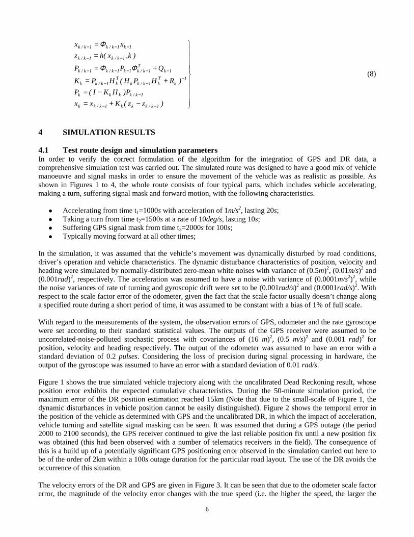
4 SIMULATION RESULTS 4.1 Test route design and simulation parameters In order to verify the correct formulation of the algorithm for the integration of GPS and DR data, a comprehensive simulation test was carried out. The simulated route was designed to have a good mix of vehicle manoeuvre and signal masks in order to ensure the movement of the vehicle was as realistic as possible. As shown in Figures 1 to 4, the whole route consists of four typical parts, which includes vehicle accelerating, making a turn, suffering signal mask and forward motion, with the following characteristics.

�� Accelerating from time t1=1000s with acceleration of 1m/s2, lasting 20s; �� Taking a turn from time t2=1500s at a rate of 10deg/s, lasting 10s; �� Suffering GPS signal mask from time t3=2000s for 100s; �� Typically moving forward at all other times;

In the simulation, it was assumed that the vehicle’s movement was dynamically disturbed by road conditions, driver’s operation and vehicle characteristics. The dynamic disturbance characteristics of position, velocity and heading were simulated by normally-distributed zero-mean white noises with variance of (0.5m)2, (0.01m/s)2 and (0.001rad)2, respectively. The acceleration was assumed to have a noise with variance of (0.0001m/s2)2, while the noise variances of rate of turning and gyroscopic drift were set to be (0.001rad/s)2 and (0.0001rad/s)2. With respect to the scale factor error of the odometer, given the fact that the scale factor usually doesn’t change along a specified route during a short period of time, it was assumed to be constant with a bias of 1% of full scale. With regard to the measurements of the system, the observation errors of GPS, odometer and the rate gyroscope were set according to their standard statistical values. The outputs of the GPS receiver were assumed to be uncorrelated-noise-polluted stochastic process with covariances of (16 m)2, (0.5 m/s)2 and (0.001 rad)2 for position, velocity and heading respectively. The output of the odometer was assumed to have an error with a standard deviation of 0.2 pulses. Considering the loss of precision during signal processing in hardware, the output of the gyroscope was assumed to have an error with a standard deviation of 0.01 rad/s. Figure 1 shows the true simulated vehicle trajectory along with the uncalibrated Dead Reckoning result, whose position error exhibits the expected cumulative characteristics. During the 50-minute simulation period, the maximum error of the DR position estimation reached 15km (Note that due to the small-scale of Figure 1, the dynamic disturbances in vehicle position cannot be easily distinguished). Figure 2 shows the temporal error in the position of the vehicle as determined with GPS and the uncalibrated DR, in which the impact of acceleration, vehicle turning and satellite signal masking can be seen. It was assumed that during a GPS outage (the period 2000 to 2100 seconds), the GPS receiver continued to give the last reliable position fix until a new position fix was obtained (this had been observed with a number of telematics receivers in the field). The consequence of this is a build up of a potentially significant GPS positioning error observed in the simulation carried out here to be of the order of 2km within a 100s outage duration for the particular road layout. The use of the DR avoids the occurrence of this situation. The velocity errors of the DR and GPS are given in Figure 3. It can be seen that due to the odometer scale factor error, the magnitude of the velocity error changes with the true speed (i.e. the higher the speed, the larger the

7

error). The heading errors from GPS and the gyroscope are shown in Figure 4. It should be noted that since vibration and temperature affect the gyroscope bias drift, the resulting heading error may fluctuate with time (i.e. not necessarily always increase). In the simulation, because the minimum vehicle speed was set to 5 m/s, the expected corresponding maximum GPS heading error should be less than 5 degrees (note that a larger GPS heading error should occur at relatively low speeds that result in distances within the GPS error envelope at various time intervals). The process of making a turn was simulated assuming a constant rate and according to the expression given below:

∆

∆

e v H t dt

n v H t dt

v v

t

v

t

v

= +�

= � +

sin( )

cos( )

ω

ω

0

0

(9)

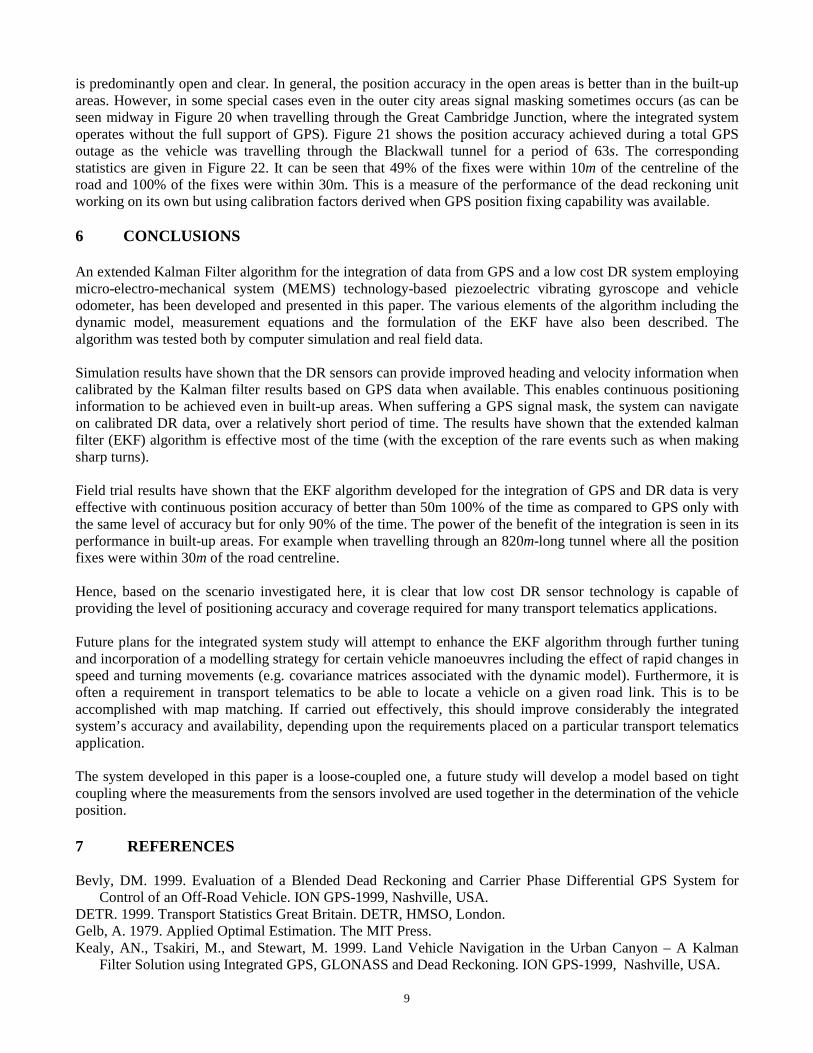
4.2 Results This section presents the results of the analysis carried out on the output of the Extended Kalman Filter (EKF) using simulated data in order to study the internal consistency and correct formulation of the algorithm, before using it with real field data. The performance of the EKF algorithm has been assessed by comparing the recovered parameters to the corresponding input values. Figure 5 shows the easting error curves for the integrated (GPS/DR) system and GPS. The impact of vehicle turning and acceleration can be seen clearly in the form of worsening system errors. A similar observation is made with respect to the northing component. However, in general the output of the EKF algorithm is very close to the GPS accuracy, is smoother and increases the availability of positioning accuracy compared to either of the systems used in stand-alone mode. This should be compared to the corresponding easting and northing errors for the uncalibrated DR data, which build up to 10 and 12 km after the 50-minute simulation period. The velocity error curves for GPS and the integrated (GPS/DR) system are shown in Figure 6. It can be seen that as expected the EKF algorithm recovered the velocity of the vehicle close to that based on GPS only, but much smoother. The impact of acceleration on the recovery of velocity can be clearly seen at around epoch 1000s when the vehicle begins to accelerate. This is due to the inability of the model to take account of non-uniform motion. The velocity of the vehicle from the DR component is smoother than that from GPS, but the scale factor of the odometer creates a jump resulting in a near constant offset. The heading error curves for the integrated (GPS/DR) and DR sensors are shown in Figure 7. The GPS heading error is considerably low when available. This is because of the assumption that the vehicle moves at a relatively high speed. It can be seen also that the heading derived from the rate gyroscope fluctuates with time because of operational environment characteristics. The gyro drift can sometimes result in an error of more than 30 degrees over the 50-minute simulation period. For the integrated system, it can be seen that heading error is much smaller compared to the gyroscope heading. However, due to the difficulty of modelling correctly all types of manoeuvres, the recovered accuracy sometimes deteriorates significantly during certain activities. Both acceleration and turning can lead to significant errors in the recovered heading. However, it should be noted that the simulation parameters selected here to a large extent represent the worst case scenario in terms of vehicle manoeuvres and that in reality such cases occur but infrequently. Figure 8 shows the difference between the true and the recovered odometer scale factor, which is of the order of 10-3 (note that when the vehicle manoeuvres, the error becomes slightly worse). The gyro scale factor was also recovered with the same level of accuracy. This shows that the input errors applied to the true scale factor values have been recovered accurately by the EKF algorithm. The simulation exercise has on the whole verified that the EKF formulation is valid (with the exception of rare occurrences). The algorithm was then used to process real field data captured during an experimental investigation in the Greater London area.

8

5 FIELD DATA RESULTS

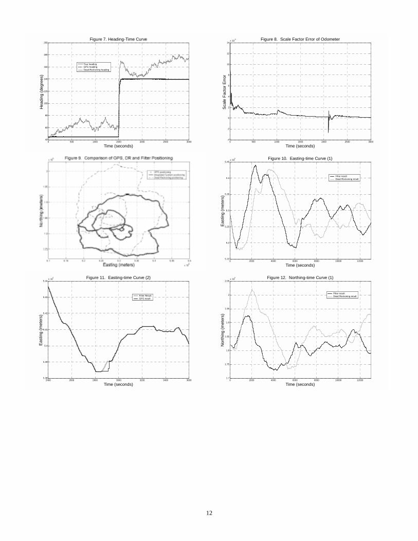
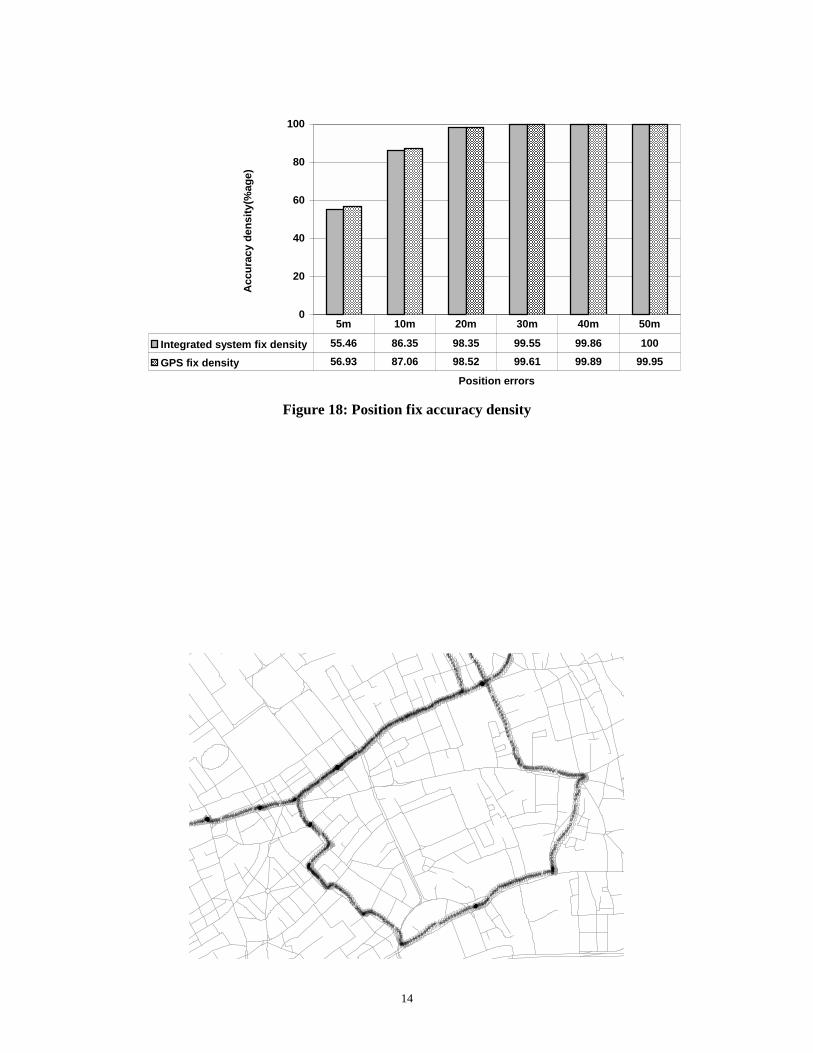
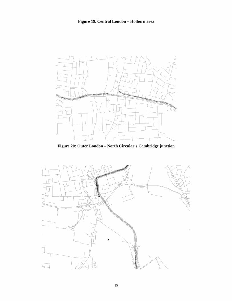
In order to carry out a credible and realistic assessment and characterisation of the performance of the integrated system, a comprehensive field test was carried out in the Grater London area in January 2002. A test vehicle was equipped with a navigation platform consisting of a 12-channel single frequency GPS receiver, a low-cost MEMS rate gyroscope and the interfaces required to connect to the vehicle speed sensor (odometer) and back-up indicator. The route in London was chosen carefully to have a good mix of important spatial urban characteristics including open spaces, urban canyons, tall buildings, tunnels, bridges, and potential sources of electromagnetic interference. Temporal consideration included capturing data to sample the temporal variation in the geometry of the GPS satellite constellation. Figure 9 shows positioning results from GPS, DR and the integrated (GPS/DR) system. The easting components from DR and GPS are given in Figures 10 and 11. The corresponding results for the northing component are given in Figures 12 and 13. It can be seen that the DR positioning is continuous with an error that accumulates over time. GPS positioning has discontinuity when suffering signal masking during the periods 2855s to 2941s and 3383s to 3437s. The results show that the integrated system based on the extended Kalman Filter exploits the strong points of both GPS (high precision and long term stability) and DR (short term stability and continuity) to provide the required availability of positioning accuracy. The velocity curves shown in Figure 14 show that the output of the EKF algorithm, as expected, is very close to GPS derived velocities when available (see the horizontal dilution of precision, HDOP values on the same figure). DR derived velocity exhibits similar accuracy with the GPS derived velocity. There is only a slight difference due to the scale factor error. When GPS suffers a signal mask or loss of lock, the odometer-derived velocity is used in the integrated system. The heading-time curve for the integrated system is compared with that of GPS and DR in Figures 15 and 16 respectively. It is interesting to note that when the geometric configuration indicator, HDOP, is greater than 100, the heading from GPS is unchanged, which can be seen in Figure 15. At other times, the GPS derived heading changes rapidly and within the system error range. DR derived velocity keeps the basic shape of the heading, but its error accumulates rapidly with time due to the gyroscope drift, which can be seen in Figure 16. If uncalibrated, the error can reach as much as 50 degrees in about 1000s. Compared to both GPS and DR derived heading, the heading derived from the integrated system has a higher precision. When GPS is available, the integrated system smoothes the effects of the GPS random noise and calibrates the drift and scale factor of the rate gyroscope. When GPS is not available, the integrated system uses the heading from the gyroscope together with the calibration data based on GPS for higher accuracy (Figure 16). In order to study the level of coverage (ability to obtain a position fix) and accuracy (position fixing with a desired level of accuracy) offered by GPS and the integrated system, the position fixing data was overlaid onto a digital London road network base map shown in Figure 17. The statistics generated showed that GPS coverage was available over 90% of the mission duration, while that of the integrated system was 100%. The longest period of GPS outage was 100s. The accuracy assessment was carried out by comparing both GPS positions and the EKF algorithm results with the digital map at a scale of 1:1250 (equivalent to a minimum plottable error of 1.25m). Furthermore, the analysis was carried out in defined accuracy bands of 5m, 10m, 20m, 30m, 40m and 50m with respect to the centreline of the road. From Figure 18, it can be seen that GPS and the integrated system have similar actual fix density, where more than 55% are in 5m of accuracy and almost 100% are within 50m. Note however, that GPS has 90% coverage while the integrated system had 100% coverage. On the basis of this, it is clear that the integrated (GPS/DR) system employing low cost DR devices performs better than GPS alone in providing continuous positioning with an accuracy of better than 50m. In order to carry out a more detailed analysis, some typical parts of the test route have been looked at in greater detail. Figure 19 shows the situation when travelling in the Holborn area of Central London that is heavily built-up with very narrow roads. Figure 20 shows results from the North Circular Road in the outskirts of London that

9

is predominantly open and clear. In general, the position accuracy in the open areas is better than in the built-up areas. However, in some special cases even in the outer city areas signal masking sometimes occurs (as can be seen midway in Figure 20 when travelling through the Great Cambridge Junction, where the integrated system operates without the full support of GPS). Figure 21 shows the position accuracy achieved during a total GPS outage as the vehicle was travelling through the Blackwall tunnel for a period of 63s. The corresponding statistics are given in Figure 22. It can be seen that 49% of the fixes were within 10m of the centreline of the road and 100% of the fixes were within 30m. This is a measure of the performance of the dead reckoning unit working on its own but using calibration factors derived when GPS position fixing capability was available. 6 CONCLUSIONS

An extended Kalman Filter algorithm for the integration of data from GPS and a low cost DR system employing micro-electro-mechanical system (MEMS) technology-based piezoelectric vibrating gyroscope and vehicle odometer, has been developed and presented in this paper. The various elements of the algorithm including the dynamic model, measurement equations and the formulation of the EKF have also been described. The algorithm was tested both by computer simulation and real field data. Simulation results have shown that the DR sensors can provide improved heading and velocity information when calibrated by the Kalman filter results based on GPS data when available. This enables continuous positioning information to be achieved even in built-up areas. When suffering a GPS signal mask, the system can navigate on calibrated DR data, over a relatively short period of time. The results have shown that the extended kalman filter (EKF) algorithm is effective most of the time (with the exception of the rare events such as when making sharp turns). Field trial results have shown that the EKF algorithm developed for the integration of GPS and DR data is very effective with continuous position accuracy of better than 50m 100% of the time as compared to GPS only with the same level of accuracy but for only 90% of the time. The power of the benefit of the integration is seen in its performance in built-up areas. For example when travelling through an 820m-long tunnel where all the position fixes were within 30m of the road centreline. Hence, based on the scenario investigated here, it is clear that low cost DR sensor technology is capable of providing the level of positioning accuracy and coverage required for many transport telematics applications. Future plans for the integrated system study will attempt to enhance the EKF algorithm through further tuning and incorporation of a modelling strategy for certain vehicle manoeuvres including the effect of rapid changes in speed and turning movements (e.g. covariance matrices associated with the dynamic model). Furthermore, it is often a requirement in transport telematics to be able to locate a vehicle on a given road link. This is to be accomplished with map matching. If carried out effectively, this should improve considerably the integrated system’s accuracy and availability, depending upon the requirements placed on a particular transport telematics application. The system developed in this paper is a loose-coupled one, a future study will develop a model based on tight coupling where the measurements from the sensors involved are used together in the determination of the vehicle position. 7 REFERENCES Bevly, DM. 1999. Evaluation of a Blended Dead Reckoning and Carrier Phase Differential GPS System for

Control of an Off-Road Vehicle. ION GPS-1999, Nashville, USA. DETR. 1999. Transport Statistics Great Britain. DETR, HMSO, London. Gelb, A. 1979. Applied Optimal Estimation. The MIT Press. Kealy, AN., Tsakiri, M., and Stewart, M. 1999. Land Vehicle Navigation in the Urban Canyon – A Kalman

Filter Solution using Integrated GPS, GLONASS and Dead Reckoning. ION GPS-1999, Nashville, USA.

10

Krakiwsky, E.J., Harris, C.B. and Wong, R.V.C. 1988. A Kalman filter for integrating dead reckoning, map matching and GPS positioning. In: Proceddings of IEEE Position Location and Navigation Symposium, 39-46.

Ochieng, WY., Noland, RB., Polak, JW., Zhao, L., Briggs, D., Gulliver, J,. Crookell, A., Evans, R., Walker, R. and Randolph, W. 2002. Integration of GPS and Dead Reckoning for Real Time Vehicle Performance and Emissions Monitoring. Accepted for Publication in the GPS Solutions Journal.

Sheridan, K and Ochieng, W.Y. 2001. VPEMS Performance Targets. Working paper, Imperial College London. Stephen, J. 2000. Operation of an Integrated Vehicle Navigation System in a Simulated Urban Canyon. ION

GPS 2000, Salt Lake City, USA. Stephen, J. 2000. Development of A Multi-Sensor GNSS Based Vehicle Navigation System. UCGE Reports

Number 20140, University of Calgary, Canada. Wood, C. and Mace, O. 2001. Vehicle positioning in Urban Environments. GPS World Online, July.

11

5 5.5 6 6.5 7 7.5 8 8.5 9 9.5

x 104

-1

-0.5

0

0.5

1

1.5

2

2.5

3

3.5x 104 Figure 1. Vehicle Trajectory

Easting (meters)

Nor

thin

g (m

eter

s)

True trajectory Dead Reckoning fixing

0 500 1000 1500 2000 2500 3000

0

2000

4000

6000

8000

10000

12000

14000

16000

Time (seconds)

Posi

tion

Erro

r (m

eter

s)

Figure 2. Position Errors

GPS position error Dead Reckoning position error

0 500 1000 1500 2000 2500 3000-2

-1.5

-1

-0.5

0

0.5

1

1.5

2

2.5Figure 3. Velocity Error

Time (seconds)

Velo

city

Erro

r (m

/s)

GPS velocity error Dead-Reckoning velocity error

0 500 1000 1500 2000 2500 3000-5

0

5

10

15

20

25

30

35

40

45Figure 4. Heading Error

Time (seconds)

Hea

ding

erro

r (de

gree

s)

GPS heading error Dead-Reckoning heading error

0 500 1000 1500 2000 2500 3000-100

-80

-60

-40

-20

0

20

40

60

80

100Figure 5. Easting Error

Time (seconds)

East

ing

Erro

r (m

eter

s)

GPS east error Filter Result east error

0 500 1000 1500 2000 2500 3000-5

-4

-3

-2

-1

0

1

2

3

4

5Figure 6. Velocity Error

Time (seconds)

Velo

city

Erro

r (m

/s)

GPS velocity error Filter Result velocity error

12

0 500 1000 1500 2000 2500 300040

60

80

100

120

140

160

180

200Figure 7. Heading-Time Curve

Time (seconds)

Hea

ding

(deg

rees

)

True heading GPS heading Dead-Reckoning heading

0 500 1000 1500 2000 2500 3000-4

-2

0

2

4

6

8

10

12

14x 10-3 Figure 8. Scale Factor Error of Odometer

Time (seconds)

Scal

e Fa

ctor

Erro

r

0 2000 4000 6000 8000 10000 120005.15

5.2

5.25

5.3

5.35

5.4

5.45x 105 Figure 10. Easting-time Curve (1)

Time (seconds)

East

ing

(met

ers)

Filter result Dead Reckoning result

2400 2600 2800 3000 3200 3400 36005.38

5.39

5.4

5.41

5.42

5.43

5.44x 105 Figure 11. Easting-time Curve (2)

Time (seconds)

East

ing

(met

ers)

Filter ResultGPS result

0 2000 4000 6000 8000 10000 120001.7

1.75

1.8

1.85

1.9

1.95

2

2.05x 105

Time (seconds)

Nor

thin

g (m

eter

s)

Figure 12. Northing-time Curve (1)

Filter result Dead Reckoning result

13

2400 2600 2800 3000 3200 3400 36001.73

1.74

1.75

1.76

1.77

1.78

1.79

1.8

1.81

1.82

1.83x 105 Figure 13. Northing-time Curve

Time (seconds)

Nor

thin

g (m

eter

s)

Filter ResultGPS result

2800 2900 3000 3100 3200 3300 3400 3500

0

5

10

15

20

25

30Figure 14. Velocity-Time Curve

Time (secons)

Velo

city

(m/s

)

GPS velocity Filter Result HDOP Odometer velocity

2800 2900 3000 3100 3200 3300 3400 35000

50

100

150

200

250

300

350Figure 15. Heading-Time Curve

Time (seconds)

Hea

ding

(deg

ree)

GPS Heading Integrated system headingHDOP

2000 2500 3000 3500 4000 4500 50000

50

100

150

200

250

300

350

Figure 16. Heading-time Curve

Time (seconds)

Hea

ding

(deg

ree)

Filter Result Dead Reckoning result

%%%%%%%%%%%%%%%%%%%%%%%%%%%%%%%%%%%%%%%%%%%%%%%%%%%%%%%%%%%%%%%%%%%%%%%%%%%%%%%%%%%%%%%%%%%%%%%%%%%%%%%%%%%%%%%%%%%%%%%%%%%%%%%%%%%%%%%%%%%%%%%%%%%%%%%%%%%%%%%%%%%%%%%%%%%%%%%%%%%%%%%%%%%%%%%%%%%%%%%%%%%%%%%%%%%%%%%%%%%%%%%%%%%%%%%%%%%%%%%%%%%%%%%%%%%%%%%%%%%%%%%%%%%%%%%%%%%%%%%%%%%%%%%%%%%%%%%%%%%%%%%%%%%%%%%%%%%%%%%%%%%%%%%%%%%%%%%%%%%%%%%%%%%%%%%%%%%%%%%%%%%%%%%%%%%%%%%%%%%%%%%%%%%%%

%%%%%%%%%%%%%%%%%%%%%%%%%%%%

%%%%%%%%%%%%%%%%%%%%%%%%%%%%%

%%%%%%%%%%%%%%%%%%%%%%%%%%%%%%%%%%%%%%%%%%%%%%%%%%%%%%%%%%%%%%%%%

%%%%%%%%%%%%%%%%%%%%%%%%%%%%%%%%%%%%%%%%%%%%%%%%%%%%%%%%%%%%%%%%%%%%%%%%%%%%%%

%%%%%%%%%%%%%%%%%%%%%%%%%%%%%%%%%%%%%%%%%%%%%%%%%%%%

%%%%%%%%%%%%%%%%%%%%%%%%%

%%%%%%%%%%%%%%%%%%%%%%%%%%%%%

%%%%%%%%%%%%%%%%%%%%%%%%%%%%

%%%%%%%%%%%%%%%%%%%%%%%%%%%%%%%%%%%%%%%%%%%%%%%%%%%%%%%%%%%%%%%%%%%%%%%%%%%%%%%%%%%

%%%%%%%%%%%%%%%%%%%%%%%%%%%%%%%%%%%%%%%%%%%%%%%%%%%%%%%%%%%%%%%%%%%%%%%%%%%%%%%%%%%%%%

%%%%%%%%%%%%%%%%%%%%%%%%%%%%%%%

%%%%%%%%%%%%%%%%%%%%%%%%%%%%%%%%%%%%%

%%%%%%%%%%%%%%%%%%%%%%%%%%%%%%%%%%%%%%%%%%

%%%%%%%%%%%%%%%%%%%%%%%%%%%%%%%%%%%%%%%%%%%%%%%%%%%%%%%%%%%%%%%%%%%%%%%%%%%%%%%%%%%%%%%%%%%%%%%%%%%%%%%%%%%%%%

%%%%%%%%%%%%%%%%%%%%%%%%%%%%%%%%%%%%%%%%%%%%%%%%%%%%%%%%%%%%%%%%%%%%%%

%%%%%%%%%%%%%%%%%%%%%%%%%

%%%%%%%%%%%%%%%%%%%%%%%%%%%%%

%%%%%%%%%%%%%%%%%%%%%%%%%%%%%%

%%%%%%%%%%%%%%%%%%%%%%%%%%%%%%%%%%%%%%%%%%%%%%%%%%%

%%%%%%%%%%%%%%%%%%%%%%%%%%%%%%%%%%%%%%%%%%%%%%%%%%%%%%

%%%%%%%%%%%%%%%%%%%%%%%%%%%%%%%%%%%

%%%%%%%%%%%%%%%%%%%%%%%%%%%%%%%%%%%%%%%%%%%%%%%%%%%%%%%%%%%%%%%%%%%%%%%%%%%%%%%%%%%%%%%%%%%%%%%%%%%%%%%%%%%%%%%%%%%%%%%%%%%%%%%%%%%%%%%%%%%%%%%%%%%%%%%%%%%%%%%%%%%%%%%%%%%%%%%%%%%%%%%%%%%%%%%%%%

%%%%%%%%%%%%%%%%%%%%%%%%%%%%%%%%%%%%%%%%%%%%%%%%%%%%%%%%%%%%%%%%%%%%%%%%%%%%%%%%%%%%%%%%%%%%%%%%%%%%%%%%%%%%%%%%%%%%%%%%%%%%%%%%%%%%%%%%%%%%%%%%%%%%%%%%%%%%%%%%%%%%%%%%%%%%%%%%%%%%%%%%%%%%%%%%%%%%%%%%%%%%%%%%%%%%%%%%%%%%%%%%%%%%%%%%%%%%%%%%%%%%%%%%%%%%%%%%%%%%%%%%%%%%%%%%%%%%%%%%%%%%%%%%%%%%%%%%%%%%%%%%%%%%%%%%%%%%%%%%%%%%%%%%%%%%%%%%%%%%%%%%%%%%%%%%%%%%%%%%%%%%%%%%%%%%%%%%%%%%%%%%%%%%%%%%%%%%%%%%%%%%%%%%%%%%%%%%%%%%%%%%%%%%%%%%%%%%%%%%%%%%%%%%%%%%%%%%%%%%%%%%%%%%%%%%%%%%%%%%%%%%%%%%%%%%%%%%%%%%%%%%%%%%%%%%%%%%%%%%%%%%%%%%%%%%%%%%%%%%%%%%%%%%%%%%%%%%%%%%%%%%%%%%%%%%%%%%%%%%%%%%%%%%%%%%%%%%%%%%%%%%%%%%%%%%%%%%%%%%%%%%%%%%%%%%%%%%%%%%%%%%%%%%%%%%%%%%%%%%%%%%%%%%%%%%%%%%%%%%%%%%%%%%%%%%%%%%%%%%%%%%%%%%%%%%%%%%%%%%%%%%%%%%%%%%%%%%%%%%%%%%%%%%%%%%%%%%%%%%%%%%%%%%%%%%%%%%%%%%%%%%%%%%%%%%%%%%%%%%%%%%%%%%%%%%%%%%%%%%%%%%%%%%%%%%%%%%%%%%%%%%%%%%%%%%%%%%%%%%%%%%%%%%%%%%%%%%%%%%%%%%%%%%%%%%%%%%%%%%%%%%%%%%%%%%%%%%%%%%%%%%%%%%%%%%%%%%%%%%%%%%%%%%%%%%%%%%%%%%%%%%%%%%%%%%%%%%%%%%%%%%%%%%%%%%%%%%%%%%%%%%%%%%%%%%%%%%%%%%%%%%%%%%%%%%%%%%%%%%%%%%%%%%%%%%%%%%%%%%%%%%%%%%%%%%%%%%%%%%%%%%%%%%%%%%%%%%%%%%%%%%%%%%%%%%%%%%%%%%%%%%%%%%%%%%%%%%%%%%%%%%%%%%%%%%%%%%%%%%%%%%%%%%%%%%%%%%%%%%%%%%%%%%%%%%%%%%%%%%%%%%%%%%%%%%%%%%%%%%%%%%%%%%%%%%%%%%%%%%%%%%%%%%%%%%%%%%%%%%%%%%%%%%%%%%%%%%%%%%%%%%%%%%%%%%%%%%%%%%%%%%%%%%%%%%%%%%%%%%%%%%%%%%%%%%%%%%%%%%%%%%%%%%%%%%%%%%%%%%%%%%%%%%%%%%%%%%%%%%%%%%%%%%%%%%%%%%%%%%%%%%%%%%%%%%%%%%%%%%%%%%%%%%%%%%%%%%%%%%%%%%%%%%%%%%%%%%%%%%%%%%%%%%%%%%%%%%%%%%%%%%%%%%%%%%%%%%%%%%%%%%%%%%%%%%%%%%%%%%%%%%%%%%%%%%%%%%%%%%%%%%%%%%%%%%%%%%%%%%%%%%%%%%%%%%%%%%%%%%%%%%%%%%%%%%%%%%%%%%%%%%%%%%%%%%%%%%%%%%%%%%%%%%%%%%%%%%%%%%%%%%%%%%%%%%%%%%%%%%%%%%%%%%%%%%%%%%%%%%%%%%%%%%%%%%%%%%%%%%%%%%%%%%%%%%%%%%%%%%%%%%%%%%%%%%%%%%%%%%%%%%%%%%%%%%%%%%%%%%%%%%%%%%%%%%%%%%%%%%%%%%%%%%%%%%%%%%%%%%%%%%

%%%%%%%%%%%%%%%%%%%%%%%%%%%%%%%%%%%%%%%%%%%%%%%%%%%%%%%%%%%%%%%%%%%%%%%%%%%%%%%%%%%%%%%%%%%%%%%%%%%%%%%%%%%%%%%%%%%%%%%%%%%%%%%%%%%%%%%%%%%%%%%%%%%%%%%%%%%%%%%%%%%%%%%%%%%%%%%%%%%%%%%%%%%%%%%%%%%%%%%%%%%%%%%%%%%%%%%%%%%%%%%%%%%%%%%%%%%%%%%%%%%%%%%%%%%%%%%%%%%%%%%%%%%%%%%%%%%%%%%%%%%%%%%%%%%%%%%%%%%%%%%%%%%%%%%%%%%%%%%%%%%%%%%%%%%%%%%%%%%%%%%%%%%%%%%%%%%%%%%%%%%%%%%%%%%%%%%%%%%%%%%%%%%%%%%%%%%%%%%%%%%%%%%%%%%%%%%%%%%%%%%%%%%%%%%%%%%%%%%%%%%%%%%%%%%%%%%%%%%%%%%%%%%%%%%%%%%%%%%%%%%%%%%%%%%%%%%%%%%%%%%%%%%%%%%%%%%%%%%%%%%%%%%%%%%%%%%%%%%%%%%%%%%%%%%%%%%%%%%%%%%%%%%%%%%%%%%%%%%%%%%%%%%%%%%%%%%%%%%%%%%%%%%%%%%%%%%%%%%%%%%%%%%%%%%%%%%%%%%%%%%%%%%%%%%%%%%%%%%%%%%%%%%%%%%%%%%%%%%%%%%%%%%%%%%%%%%%%%%%%%%%%%%%%%%%%%%%%%%%%%%%%%%%%%%%%%%%%%%%%%%%%%%%%%

%%%%%%%%%%%%%%%%%%%%%%%%%%%%%%%%%%%%%%%%%%%%%%%%%%%%%%%%%%%%%%%%%%%%%%%%%%%%%%%%%%%%%%%%%%%%%%%%%%%%%%%%%%%%%%%%%%%%%%%%%%%%%%%%%%%%%%%%%%%%%%%%%%%%%%%%%%%%%%%%%%%%%%%%%%%%%%%%%%%%%%%%%%%%%%%%%%%%%%%%%%%%%%%%%%%%%%%%%%%%%%%%%%%%%%%%%%%%%%%

%%%%%%%%%%%%%%%%%%%%%%%%%%%%%%%%%%%%%%%%%%%%%%%%%%%%%%%%%%%%%%%%

%%%%%%%%%%%%%%%%%%%%%%%%%%%%%%%%%%%%%%%%%%%%%%%%%%%%%%

%%%%%%%%%%%%%%%%%%%%%%%%%%%%%%%%%%%%%%%%%%%%%%%%%%%%%%%%%

%%%%%%%%%%%%%%%%%%%%%%%%%%%%%%%%%%%%%%%%%%%%%%%%%%%%%%%%%%%%%%%%%%%

%%%%%%%%%%%%%%%%%%%%%%%%%%%%%%%%%%

%%%%%%%%%%%%%%%%%%%%%%%%%%%%%%%%%%%%%%%%%%%%%%%%%%%%%%%%%%%%%%%%%%%%%%%%%%%%%%%%%%%%%%%%%%%%%%%%%%%%%%%%%%%%%%%%%%%%%%%%%%%%%%%%%%%%%%%%%%%%%%%%%%%%%%%%%%%%%%%%%%%%%%%%%%%%%%%%%%%%%%%%%%%%%%%%%%%%%%%%%%%%%%%%%%%%%%%%%%%%%%%%%%%%%%%%%%%%%%%%%%%%%%%%%%%%%%%%%%%%%%%%%%%%%%%%%%%%%%%%%%%%%%%%%%%%%%%%%%%%%%%%%%%%%%%%%%%%%%%%%%%%%%%%%%%%%%%%%%%%%%%%%%%%%%%%%%%%%%%%%%%

%%%%%%%%%%%%%%%%%%%%%%%%%%%%%%%%%%%%%%%%%%%%%%%%%%%%%%%%%%%%%%%

%%%%%%%%%%%%%%%%%%%%%%%%%%%%%%%%%%%%%%%%%%%%%%%%%%%%%%%%%%%%%%%%%%%%%%%%%%%%%%%%%%%%%%%%%%%%%%%%%%%%%%%%%%%%%%%%%%%%%%%%%%%%%%%%%%%%%%%%%%%%%%%%%%%%%%%%%%%%%%%%%%%%%%%%%%%%%%%%%%%%%%%%%%%%%%%%%%%%%%%%%%%%%%%%%%%%%%%%%%%%%%%%%%%%%%%%%%%%%%%%%%%%%%%%%%%%%%%%%%

%%%%%%%%%%%%%%%%%%%%%%%%%%%%%%%%%%%%%%%%%%%%%%%%%%%%%%%%%%%%%%%%%%%%%%%%%%%%%%%%%%%%%%%%%%%%%%%%%%%%%%%%%%%%%%%%%%%

%%%%%%%%%%%%%%%%%%%%%%%%%%%%%%%%%%%%%%%%%%%%%%%%%%%%%%%%

%%%%%%%%%%%%%%%%%%%%%%%%%%%%%%%%%%%%%%%%%%%%%%%%%%%%%%%%%%%%%%%%%%%%%%%%%%%%%%%%%%%%%%%%%%%%%%%%%%%%%%%%%%%%%%%%%%%%%%%%%%%%%%%%%%%%%%%%%%%%%%%%%%%%%%%%%%%%%%%%%%%%%%%%%%%%%%%%%%%%%%%%%%%%%%%%%%%%%%%%

%%%%%%%%%%%%%%%%%%%%%%%%%%%%%%%%%%%%%%%%%%%%%%%%%%%%%

%%%%%%%%%%%%%%%%%%%%%%%%%%%%%%%%%%%%%%%%%%%%%%%%%%%

%%%%%%%%%%%%%%%%%%%%%%%%%%%%%%%%%%%%%%%%%%%%%%%%%%%%%%%%%%%%%%%%%%%%%%%%%%%%%%%%%%%%%%%%%%%%%%%%%%%%%%%%%%%%%%%%%%%%%%%%%%%%%%%%%%%%%%%%%%%%%%%%%%%%%%%%%%%%%%%%%%%%%%%%%%%%%%%%%%%%%%%%%%%%%%%%%%%%%%%%%%%%%%%%%%%%%%%%%%%%%%%%%%%%%%%%%%%%%%%%%%%%%%%%%%%%%

%%%%%%%%%%%%%%%%%%%%%%%%%%%%%%%%%%%%%%%%%%%%%%%%%%%%%%%%%%%%%%%%%%%%%%%%%%%%%%%%%%%%%%%%%%%%%%%%%%%%%%%%%%%%%%%%%%%%%%%%%%%%%%%%%%%%%%%%%%%%%%%%%%%%%%%%%%%%%%%%%%%%%%%%%%%%%%%%%%%%%%%%%%%%%%%%%%%%%%%%%%%%%%%%%%%%%%%%%%%%%%%%%%%%%%%%%%%%%%%%%%%%%%%%%%%%%%%%%%%%%%%%%%%%%%%%%%%%%%%%%%%%%%%%%%%%%%%%%%%%%%%%%%%%%%%%%%%%%%%%%%%%%%%%%%%%%%%%%%%%%%%%%%%%%%%%%%%%%%%%%%%%%%%%%%%%%%%%%%%%%%%%%%%%%%%%%%%%%%%%%%%%%%%%%%%

%%%%%%%%%%%%%%%%%%%%%%%%%%%%%%%%%%%%%%%%%%%%%%%%%%%%%%%%%%%%%%%%%%%%%%%%%%%%%%%%%%%%%%%%%%%%%%%%%%%%%%%%%%%%%%%%%%%%%%%%%%%%%%%%%%%%%%%%%%%%%%%%%%%%%%

%%%%%%%%%%%%%%%%%%%%%%%%%%%%%%%%%%%%%%%%%%%%%%%%%%%%%%%%%%%%%%%%%%%%%%%%%%%%%%%%%%%%%%%%%%%%%%%%%%%%%%%%%%%%%%%%%%%%%%%%%%%%%%%%%%%%%%%%%%%%%%%%%%%%%%%%%%%%%%%%%%%%%%%%%%%%%%%%%%%%%%%%%%%%%%%%%%%%%%%%%%%%%%%%%%%%%%%%%%%%%%%%%%%%%%%%%%%%%%%%%%%%%%%%%%%%%%%%%%%%%%%%%%%%%%%%%%%%%%%%%%%%%%%%%%%%%%%%%%%%%%%%%%%%%%%%%%%%%%%%%%%%%%%%%%%%%%%%%%%%%%%%%%%%%%%%%%%%%%%%%%%%%%%%%%%%%%%%%%%%%%%%%%%%%%%%%%%%%%%%%%%%%%%%%%%%%%%%%%%%%%%%%%%%%%%%%%%%%%%%%%%%%%%%%%%%%%%%%%%%%%%%%%%%%%%%%%%%%%%%%%%%%%%%%%%%%%%%%%%%%%%%%%%%%%%%%%%%%%%%%%%%%%%%%%%%%%%%%%%%%%%%%%%%%%%%%%%%%%%%%%%%%%%%%%%%%%%%%%%%%%%%%%%%%%%%%%%%%%%%%%%%%%%%%%%%%%%%%%%%%%%%%%%%%%%%%%%%%%%%%%%%%%%%%%%%%%%%%%%%%%%%%%%%%%%%%%%%%%%%%%%%%%%%%%%%%%%%%%%%%%%%%%%%%%%%%%%%%%%%%%%%%%%%%%%%%%%%%%%%%%%%%%%%%%%%%%%%%%%%%%%%%%%%%%%%%%%%%%%%%%%%%%%%%%%%%%%%%%%%%%%%%%%%%%%%%%%%%%%%%%%%%%%%%%%%%%%%%%%%%%%%%%%%%%%%%%%%%%%%%%%%%%%%%%%%%%%%%%

%%%%%%%%%%%%%%%%%%%%%%%%%%%%%%%%%%%%%%%%%%%%%%%%%%%%%%%%%%%%%%%%%%%%%%%%%%%%%%%%%%%%%%%%%%%%%%%%%%%%%%%%%%%%%%%%%%%%%%%%%%%%%%%%%%%%%%%%%%%%%%%%%%%%%%%%%%%%%%%%%%%%%%%%%%%%%%%%%%%%%%%%%%%%%%%%%%%

%%%%%%%%%%%%%%%%%%%%%%%%%%%%%%%%%%%%%%%%%%%%%%%%%%%%%%%%%%%%%%%%%%%%%%%%%%%%%%%%%%%%%%%%%%%%%%%%%%%%%%%%%%%%%%%%%%%%%%%%%%%%%%%%%%%%%%%%%%%%%%%%%%%%%%%%%%%%%%%%%%%%%%%%%%%%%%%%%%%%%%%%%%%%%%%%

%%%%%%%%%%%%%%%%%%%%%%%%%%%%%%%%%%%%%%%%%%%%%%%%%%%%%%%%%%%%%%%%%%%%%%%%%%%%%%%%%%%%%%

%%%%%%%%%%%%%%%%%%%%%%%%%%%%%%%%%%%%%%%%%%%%%%%%%%%%%%%%%%%%%%%%%%%%%%%%%%%%%%%%%%%%%%%%%%%%%%%%%%%%%%%%%%%%%%%%%%%%%%%%%%%%%%%%%%%%%%%%%%%%%%%%%%%%%%%%%%%%%%%%%%%%%%%%%%%%%%%%%%%%%%%%%%%%%%%%%%%%%%%%%%%%%%%%%%%%%%%%%%%%%%%%%%%%%%%%%%%%%%%%%%%%%%%%%%%%%%%%%%%%%%%%%%%%%%%%%%%%%%%%%%%%%%%%%%%%%%%%%%%%%%%%%%%%

%%%%%%%%%%%%%%%%%%%%%%%%%%%%%%%%%%%%%%%%%%%%%%%%%%%%%%%%%%%%%%%%%%%%%%%%%%%%%%%%%%%%%%%%%%%%%%%%%%%%%%%%%%%%%%%%%%%%%%%%%%%%%%%%%%%%%%%%%%%%%%%%%%%%%%%%%%%%%%%%%%%%%%%%%%%%%%%%%%%%%%%%%%%%%%%

%%%%%%%%%%%%%%%%%%%%%%%%%%%%%%%%%%%%%%%%%%%%%%%%%%%%%%%%%%%%%%%%%%%%%%%%%%%%%%%%%%%%%%%%%%%%%%%%%%%%%%%%%%%%%%%%%%%%%%%%%%%%%

%%%%%%%%%%%%%%%%%%%%%%%%%%%%%%%%%%%%%%%%%%%%%%%%%%%%%%%%%%%%%%%%%%%%%%%%%%%%%%%

%%%%%%%%%%%%%%%%%%%%%%%%%%%%%%%%%%%%%%%%%%%%%%%%%%%%%%%%%%%%%%%%%%%%%%%%%%%%%%%%%%%%%%%%%%%%%%%%%%%%%%%%%%%%%%%%%%%%%%%%%%%%%%%%%%%%%%

%%%%%%%%%%%%%%%%%%%%%%%%%%%%%%%%%%%%%%%%%%%%%%%%%%%%%%%%%%%%%%%%%%%%%%%%%%%%%%%%%%%%%%%%%%%%%%%%%%%%%%%%%%%%%%%%%%%%%%%%%%%%%%%%%%%%%%%%%%%%%%%%%%%%%%%%%%%%%%%%%%%%%%%%%%%%%%%%%%%%%%%%%%%%%%%%%%%%%%%%%%%%%%%%%%%%%%%%%%%%%%%%%%%%%%%%%%%%%%%%%%%%%%%%%%%%%%%%%%%%%%%%%%%%%%%%%%%%%%%%%%%%%%%%%%%%%%%%%%%%%%%%%%%%%%%%%%%%%%%%%%%%%%%%%%%%%%%%%%%%%%%%%%%%%%%%%%%%%%%%%%%%%%%%%%%%%%%%%%%%%%%%%%%%%%%%%%%%%%%%%%%%%%%%%%%%%%%%%%%%%%%%%%%%%%%%%%%%%%%%%%%%%%%%%%%%%%%%%%%%%%%%%%%%%%%%%%%%%%%%%%%%%%%%%%%%%%%%%%%%%%%%%%%%%%%%%%%%%%%%%%%%%%%%%%%%%%%%%%%%%%%%%%%%%%%%%%%%%%%%%%%%%%%%%%%%%%%%%%%%%%%%%%%%%%%%%%%%%%%%%%%%%%%%%%%%%%%%%%%%%%%%%%%%%%%%%%%%%%%%%%%%%%%%%%%%%%%%%%%%%%%%%%%%%%%%%%%%%%%%%%%%%%%%%%%%%%%%%%%%%%%%%%%%%%%%%%%%%%%%%%%%%%%%%%%%%%%%%%%%%%%%%%%%%%%%%%%%%%%%%%%%%%%%%%%%%%%%%%%%%%%%%%%%%%%%%%%%%%%%%%%%%%%%%%%%%%%%%%%

%%%%%%%%%%%%%%%%%%%%%%%%%%%%%%%%%%%%%%%%%%%%%%%%%%%%%%%%%%%%%%%%%%%%%%%%%%%%%%%%%%%%%%%%%%%%%%%%%%%%%%%%%%%%%%%%%%%%%%%%%%%%%%%%%%%%%%%%%%%%%%%%%%%%%%%%%%%%%%%%%%%%%%%%%%%%%%%%%%%%%%%%%%%%%%%%%%%%%%%%%%%%%%%%%%%%%%%%%%%%%%%%%%%%%%%%%%%%%%%%%%%%%%%%%%%%%%%%%%%%%%%%%%%%%%%%%%%%%%%%%%%%%%%%%%%%%%%%%%%%%%%%%%%%%%%%%%%%%%%%%

%%%%%%%%%%%%%%%%%%%%%%%%%%%%%%%%%%%%%%%%%%%%%%%%%%%%%%%%%%%%%%%%%%%%%%%%%%%%%%%%%%%%%%%%

%%%%%%%%%%%%%%%%%%%%%%%%%%%%%%%%%%%%%%%%%%%%%%%%%%%%%%%%%%%%%%%%%%%%%%%%%%%%%%%%%%%%%%%%%%%%%%%%%%%%%%%%%%%%%%%%%%%%%%%%%%%%%%%%%%%%%%%%%%%%%%%%%%%%%%%%%%%%%%%%%%%%%%%%%%%%%%%%%%%%%%%%%%%%%%%%%%%%%%%%%%%%%%%%%%%%%%%%%%%%%%%%%%%%%%%%%%%%%%%%%%%%%%%%%%%%%%%%%%%%%%%%%%%%%%%%%%%%%%%%%%%%

%%%%%%%%%%%%%%%%%%%%%%%%%%%%%%%%%%%%%%%%%%%%%%%%%%%%%%%%%%%%%%%%%%%%%%%%%%%%%%%%%%%%%%%%%%%%%%%%%%%%%%%%%%%%%%%%%%%%%%%%%%%%%%%%%%%%%%%%%%%%%%%%%%%%%%%%%%%%%%%%%%%%%%%%%%%%%%%%%%%%%%%%%%%%%%%%%%%%%%%%%%%%%%%%%%%%%%%%%%%%

%%%%%%%%%%%%%%%%%%%%%%%%%%%%%%%%%%%%%%%%%%%%%%%%%%%%%%%%%%%%%%%%%%%%%%%%%%%%%%%%%%%%%%%%%%%%%%%%%%%%%%%%%%%%%%%%%%

%%%%%%%%%%%%%%%%%%%%%%%%%%%%%%%%%%%%%%%%%%%%%%%%%%%%%%%%%

%%%%%%%%%%%%%%%%%%%%%%%%%%%%%%%%%%%%%%%%%%%%%%%%%%%%%%%%%%%%%%%%%%%%%%%%%%%%%%%%%%%%%%%%%%%%%%%%%%%%%%%%%%%%%%%%%%%%%%%%%%%%%%%%%%%%%%%%%%%%%%%%%%%%%%%%%%%%%%%%%%%%%%%%%%%%%%%%%%%%%%%%%%%%%%%%%%%%%%%%%%%%%%%%%%%%%%%%%%%%%%%%%%%

%%%%%%%%%%%%%%%%%%%%%%%%%%%%%%%%%%%%%%%%%%%%

%%%%%%%%%%%%%%%%%%%%%%%%%%%%%%%%%%%%%%%%

%%%%%%%%%%%%%%%%%%%%%%%%%%%%%%%%%%%%%%%%%%%%%%%%%%%%%%%%%%%%%%%%%%%%%%%%%%%%

%%%%%%%%%%%%%%%%%%%%%%%%%%%%%%%%

%%%%%%%%%%%%%%%%%%%%%%%%%%%%%%%%%%%%%%%%%%%%%%%%%%%%%%

%%%%%%%%%%%%%%%%%%%%%%%%%%%%%%%%%%%%%%%%%%%%%%%%%

%%%%%%%%%%%%%%%%%%%%%%%%%%%%%%%%%%%%%%%%%%%%%%%%%%%%%%%%%%%%%%%%%%%%%%%%%%%%%%%%%

%%%%%%%%%%%%%%%%%%%%%%%%%%%%%%%%%%%%%%%%%%%%%%%%%%%%%%%%%%%%%%%%%%%%%%%%%%%%%%%%%%%%%%%%%%%%%%%%%%%%%%%%%%%%%%%%%%%%%%%%%%%%%%%%%%%%%%%%%%%%%%%%%%%%%%%%%%%%%%%%%%%%%%%%%%%%%%%%%%%%%%%%%%%%%%%%%%%%%%%%%%%%%%%%%%%%%%%%%%%%%%%%%%%%%%%%%%%%%%%%%%%%%%%%%%%%%%%%%%%%%%%%%%%%%%%%%%%%%%%%%%%%

%%%%%%%%%%%%%%%%%%%%%%%%%%%%%%%%%%%%%%%%%%%%%%%%%%%%%%%%%%%%%%%%%%%%%%%%%%%%%%%%%%%%%%%%%%%%%%%%%%%%%%%%%%%%%%%%%%%%%%%%%%%%%%%%%%%%%%%%%%%%%%%%%%%%%%%%%%%%%%%%%%%%%%%%%%%%%%%%%%%%%%%%%%%%%%%%%%%%%%%%%%%%%%%%%%%%%%%%%%%%%%%%%%%%%%%%%%%%%%%%%%%%%%%%%%%%%%%%%%%%%%%%%%%%%%%%%%%%%%%%%%%%%%%%%%%%%%%%%%%%%%%%%%%%%%%%%%%%%%%%%%%%%%%%%%%%%%%%%%%%%%%%%%%%%%%%%%%%%%%%%%%%%%%%%%%%%%%%%%%%%%%%%%%%%%%%%%%%%%%%%%%%%%%%%%%%%%%%%%%%%%%%%%%%%%%%%%%%%%%%%%%%%%%%%%%%%%%%%%%%%%%%%%%%%%%%%%%%%%%%%%%%%%%%%%%%%%%%%%%%%%%%%%%%%%%%%%%%%%%%%%%%%%%%%%%%%%%%%%%%%%%%%%%%%%%%%%%%%%%%%%%%%%%%%%%%%%%%%%%%%%%%%%%%%%%%%%%%%%%%%%%%%%%%%%%%%%%%%%%%%%%%%%%%%%%%%%%%%%%%%%%%%%%%%%%%%%%%%%%%%%%%%%%%%%%%%%%%%%%%%%%%%%%%%%%%%%%%%%%%%%%%%%%%%%%%%%%%%%%%%%%%%%%%%%%%%%%%%%%%%%%%%%%%%%%%%%%%%%%%%%%%%%%%%%%%%%%%%%%%%%%%%%%%%%%%%%%%%%%%%%%%%%%%%%%%%%%%%%%%%%%%%%%%%%%%%%%%%%%%%%%%%%%%%%%%%%%%%%%%%%%%%%%%%%%%%%%%%%%%%%%%%%%%%%%%%%%%%%%%%%%%%%%%%%%%%%%%%%%%%%%%%%%%%%%%%%%%%%%%%%%%%%%%%%%%%%%%%%%%%%%%%%%%%%%%%%%%%%%%%%%%%%%%%%%%%%%%%%%%%%%%%%%%%%%%%%%%%%%%%%%%%%%%%%%%%%%%%%%%%%%%%%%%%%%%%%%%%%%%%%%%%%%%%%%%%%%%%%%%%%%%%%%%%%%%%%%%%%%%%%%%%%%%%%%%%%%%%%%%%%%%%%%%%%%%%%%%%%%%%%%%%%%%%%%%%%%%%%%%%%%%%%%%%%%%%%%%%%%%%%%%%%%%%%%%%%%%%%%%%%%%%%%%%%%%%%%%%%%%%%%%%%%%%%%%%%%%%%%%%%%%%%%%%%%%%%%%%%%%%%%%%%%%%%%%%%%%%%%%%%%%%%%%%%%%%%%%%%%%%%%%%%%%%%%%%%%%%%%%%%%%%%%%%%%%%%%%%%%%%%%%%%%%%%%%%%%%%%%%%%%%%%%%%%%%%%%%%%%%%%%%%%%%%%%%%%%%%%%%%%%%%%%%%%%%%%%%%%%%%%%%%%%%%%%%%%%%%%%%%%%%%%%%%%%%%%%%%%%%%%%%%%%%%%%%%%%%%%%%%%%%%%%%%%%%%%%%%%%%%%%%%%%%%%%%%%%%%%%%%%%%%%%%%%%%%%%%%%%%%%%%%%%%%%%%%%%%%%%%%%%%%%%%%%%%%%%%%%%%%%%%%%

##################################################################################################################################################################################

######################################################################################################################################################################################################################

##################

################

##################

####################

###############################################

#######################

########################################################################

#############

#############

##############

################

#################################

#################

################################################################################

##########################################################################################

####################

##################

#########################

####################

############################

##################

################################################################

##########################################################################

#################

##############

##############

##################

###########

#############

################

#################

#######################################

#################

##########################

####################################

###################

#################################################################################################################################################################################

#####################

####################################################################################################### ##################################################################

##################################################################################################################################################################################################################

#################################################################################################################################################################################################################################################################################################################################################################################################################################################################################################################################################################################################################################################################################################################################################################################################################################################################################################################################################################

#####################################################################################################################################################################################################################################################################################################################################################################################################################

#############################################################################################################################################################################################################################################################################################################################################################################################################################################################################################################################################################################################################################################################################################################################################################################################################################################################

################

###########################################################################################################################################################################################################################

##########################

#############################################

########################

########################################

#######################################

###################

##############################################

###########################

####################

##############################################

###################################################################################################################################################################################################################################################################################################################################

####################################

#####################################

################################################################

#########################################################################################################################################################################################################################################################################################

#####################################################################

###############################

##########################################################################################################

############################################################

############################################

#############

#########################################

################################

###################################################################################################################################################################################################################################

###############################################################################################################################################################################################################################################################################################################################################################

##########################################################

####################

############

##########################################################################

##############################################################################################################################################################################################################################################################################################################################################################################################################################################################################################################################################################################################################################################################################################################################################################################################################################################################################################################

####################################

#############################

####################################################################################################################################################################

#############################################################################

#############################################################################################################################

##############################

#####################

#####################################################################################################################################################################################################################################################################################################################################################

###############################

#########################################################################

##################################################################

#################################################################################################################################

######################

#######################################################################

##########################################################

#######################################################################################

##################################################################################################################################################################################################################################################################################################################################################################################################################################################################################################################################################################################################################################################################################################################################################################################

#####################################################################################################################################################################################################

######################################################################################################################################################################

##############################################################################

###########################

###############################################################################################################################################################################################################################################################################

############################################################

#########################################################################################

#########################

###########################################################################

###############################################################################################

##########################################################

###############################################################################################################################################################################################################################################

##################

############################

##########################

#########################

###########################################################

#################

#################

###########################

########################################

##########################

#####################################

####################################################

########################################################################################################################################################################################################################################

##############################################

##########################################################################################################################################################################################################################################################################################################################################################################################################################################################################################################################################################################################################################################################################################################################################################################################################################################################################################################################################################

###############################################################################################################################################################################################################################################################################################################################################################################################################################################################################################################################

################################################################################################################################################################

Figure 17. Vehicle test trajectory

14

0

20

40

60

80

100

Position errors

Acc

urac

y de

nsity

(%ag

e)

Integrated system fix density 55.46 86.35 98.35 99.55 99.86 100

GPS fix density 56.93 87.06 98.52 99.61 99.89 99.95

5m 10m 20m 30m 40m 50m

Figure 18: Position fix accuracy density

%%%%%%%%%%%%%%%%%%%%%%%%%%%%%%%%%%%%%%%%%%%%%%%%%%%%%%

%%%%%%%%%%%%%%%%%%%%%%%%%%%%%%%%%%%%

%%%%%%%%%%%%%%%%%%%%%%%%

%%%%%%%

%%%%%%%

%%%%%%%%%%%%%%%%%%%%%%%%%%%%%%%%%%%%%%%

%%%%%%%

%%%%%%

%%%%

%%%%%

%%%%%%%%%

%%%%%%%%%%%%

%%%%%%%%%%

%%%%%%

%%% %%%%%%%%%%%%%%%%%%%%%%%%%%%

%%%%%%%%%%%%%%%%%%%%%%%%%%%%%%%%%%%%%%%%%%%%%%%%%%%%%%

%%%%%%%%%%%%%%%%%%%%%%%%%%%%%%%%%%%%%%%%%%%%%%%%%%%%%%%%%%%%%%%%%%%%%%%%%%%%%%%%%%%%%%%%%%%%%%%%%%%%%%%%%%%%%%%%%%%%%%%%%%%%%%%%%%%%%%

%%%%%

%%%%%%%%%%%%%%%%%%%%

%%%%

%%%%%

%%%%%%%%%%%%%%%%

%%%%%%%%%%%%

%%%%%%%%%%%%%%%%%%%%%

%%%%%%%%

%%%%%%%

%%%%%

%%%%%%%%%%%%%%%%%%%%%%%%%%%%%%%%%%%%%%%%%%%%%%%%%%%%%

%%%%%%%%

%%%%%%%

%%%%%%

%%%%%%%%%%%%%%%%%%%%%%%%%%%%%%%%%%%%%%%%%%%%%

%%%%%%%%%%%%

%%%%%%%

%%%%%

%%%%%

%%%%%%%%%%%%

%%%%%%%%%%

%%%%%%%%%%

%%%%%%%%%%%%%%%%%%%%%%%%%%%%%%%%%%%%%%%%%%%%%%%%%%%%%%%%%%%%%

%%%%%%%

%%%%%%%%

#####################################################

############################################## #######

############

####

#####

####

#########

#################################

####

####

###

#######

########################

#####

#####

##

### ##

########

####

###

##########

######################## ###################

#####

#

####

##

##

####

###

##############################################

#########################################################################

####

####

####

#################

###

###

####

#####

###########

######

#########

###############

####

####

#######

######

####

##################################################

#####

#######

########

###

##########################################

######

#############

####

#####

##########

#########

######

##########

###########################################################

#### ##

#####

######

15

Figure 19. Central London – Holborn area

%%%%%%%%%%%%%%%%%%%%%%%%%%%%%%%%%%%%%%%%%%%%%%%%%

%%%%%%%%%%%%%%%%%%%%%%%%%%%%%%%%%%%%%%%%%%%%%%

###### # ## # ## # # # # ############# ## # # ## # # # # ##########

## ## ## ## ## # # ## ## # # # # # # # # # # # # # # # # # # ## ###

######

#

Figure 20: Outer London – North Circular’s Cambridge junction

%%%%%%%%%%%%%%%%%%%%%%%%%%%%%%%%%%%%%%%%%%%%%%%%%%%%%%%%%%%%%%%%%%%%%%%%%%%%%%%%%%%%%%%%%%%%%%%%%%%%%%%%%%%%%%%%%%%%%%%%%%%%%%%%%%%%%%%%%%%%%%%%%%%%%%%%%%%%%%%%%%%%%%%%%%

#########################################################################################

#########################################################

########

#

##

#############

16

Figure 21: Travelling inside the Blackwall Tunnel

0

20

40

60

80

100

Position errors

Acc

urac

y D

ensi

ty(%

age)

Accuracy density 38 49 87 100

5m 10m 20m 30m

Figure 22: Accuracy fix density in tunnel