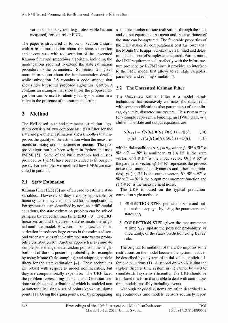
An FMI-based Framework for State and Parameter...

An FMI-based Framework for State and Parameter Estimation

Marco Bonvini, Michael Wetter, Michael D. SohnSimulation Research Group, Lawrence Berkeley National Laboratory

1 Cyclotron Road, 94720, Berkeley, CA

Abstract

This paper proposes a solution for creating a model-based state and parameter estimator for dynamic sys-tems described using the FMI standard. This workuses a nonlinear state estimation technique called un-scented Kalman filter (UKF), together with a smootherthat improves the reliability of the estimation. The al-gorithm can be used to support advanced control tech-niques (e.g., adaptive control) or for fault detection anddiagnostics (FDD). This work extends the capabilitiesof any modeling framework compliant with the FMIstandard version 1.0.

Keywords: Nonlinear State and Parameter Estima-tion; Unscented Kalman Filter (UKF); Smoothing;Functional Mockup Interface (FMI); Fault Detectionand Diagnosis (FDD)

1 Introduction

In many applications, after the system has been de-signed, controls and/or fault detection and diagnostics(FDD) algorithms are developed and deployed. Thesetechniques should be able to leverage the models de-veloped during the earlier design stages, thereby in-creasing the productivity of the overall product devel-opment. Advanced control (such as adaptive controlor model predictive control) and FDD techniques re-quire an enhanced knowledge of the system state. Forexample, the flight controller of an airplane should tryto estimate the real velocity and position of the air-craft while compensating for measurements errors andsensor noises. When dealing with dynamic system,having an enhanced knowledge about the system statemeans estimating its state variables with associated er-ror bounds.

This paper proposes a solution for creating a model-based state estimator for dynamic systems describedusing the FMI standard. This work extends the ca-pabilities of any modeling framework compliant withthe FMI standard version 1.0. The FMI is a stan-

dard that allows to embed a simulation model withina unified interface in order to couple simulation mod-els developed using different simulation programs. Al-though the FMI standard has been created mainly forco-simulation, we leverage this standard for provid-ing an algorithm that is compatible with a large num-ber of simulation and modeling platforms, includingModelica-based ones.

There are several characteristics intrinsic of anymodel-based state estimation technique. These char-acteristics are related to the model properties (e.g., theKalman filter is applicable just to linear models), theassumptions introduced when describing the probabil-ity distribution of the state variables (e.g., assumingthey are Gaussian) and the computational performanceof the underlying algorithm (e.g., the number of simu-lations or computations to be done in order to providean estimation).

The state estimation technique used in this work isthe unscented Kalman filter (UKF) [1, 2]. The UKF isable to deal with nonlinear systems and it just requiresto perform function evaluations of the model in orderto compute the evolution of its state variables and thevalue of its outputs. The UKF has less requirementsabout the knowledge of the model with respect to othernonlinear state estimation techniques. For example theextended Kalman filter needs to linearize the model[3]. The computational performances of the UKF aremodest with respect to other Monte Carlo based tech-niques (like particle filters [4]), enabling its use forreal-time applications.

The proposed work leverages the UKF techniqueand provides a state and parameter estimation algo-rithm for a dynamic system (e.g., modeled with Mod-elica or Matlab) embedded according to the FMI stan-dard as a Functional Mockup Unit (FMU). The model,once exported as FMU can be used to set up a stateand parameter estimator to

• calibrate the model during the commissioningphase in order to check if it performs as expected,

• compute a probabilistic estimation of unknown

DOI10.3384/ECP14096647

Proceedings of the 10th International ModelicaConferenceMarch 10-12, 2014, Lund, Sweden

647

variables of the system (e.g., observable but notmeasured) for control or FDD.

The paper is structured as follows. Section 2 startswith a brief introduction about the state estimationand it continues with a description of the unscentedKalman filter and smoothing algorithm, including themodifications required to extend the state estimationprocedure to the parameters. Subsection 2.5 givesmore information about the implementation details,while subsection 2.6 contains a code snippet thatshows how to use the proposed algorithm. Section 3contains an example that shows how the proposed al-gorithm can be used to identify faulty operation in avalve in the presence of measurement errors.

2 Method

The FMI-based state and parameter estimation algo-rithm consists of two components: (i) a filter for thestate and parameter estimation, (ii) a smoother that im-proves the quality of the estimation when the measure-ments are noisy and sometimes erroneous. The pro-posed algorithm has been written in Python and usesPyFMI [5]. Some of the basic methods and classesprovided by PyFMI have been extended to fit our pur-poses. For example, we modified how FMUs are exe-cuted in parallel.

2.1 State Estimation

Kalman Filter (KF) [3] are often used to estimate statevariables. However, as they are only applicable forlinear systems, they are not suited for our applications.For systems that are described by nonlinear differentialequations, the state estimation problem can be solvedusing an Extended Kalman Filter (EKF) [3]. The EKFlinearizes around the current state estimate the origi-nal nonlinear model. However, in some cases, this lin-earization introduces large errors in the estimated sec-ond order statistics of the estimated state vector proba-bility distribution [6]. Another approach is to simulatesample paths that generate random points in the neigh-borhood of the old posterior probability, for exampleby using Monte Carlo sampling, and adopting particlefilters for the state estimation [4]. These techniquesare robust with respect to model nonlinearities, butthey are computationally expensive. The UKF facesthe problem representing the state as a Gaussian ran-dom variable, the distribution of which is modeled nonparametrically using a set of points known as sigmapoints [1]. Using the sigma points, i.e., by propagating

a suitable number of state realizations through the stateand output equations, the mean and the covariance ofthe state can be captured. The favorable properties ofthe UKF makes its computational cost far lower thanthe Monte Carlo approaches, since a limited and deter-ministic number of samples are required. Furthermore,the UKF requirements fit perfectly with the infrastruc-ture provided by PyFMI since it provides an interfaceto the FMU model that allows to set state variables,parameter and running simulations.

2.2 The Unscented Kalman Filter

The Unscented Kalman Filter is a model based-techniques that recursively estimates the states (andwith some modifications also parameters) of a nonlin-ear, dynamic, discrete-time system. This system mayfor example represent a building, an HVAC plant or achiller. The state and output equations are

x(tk+1) = f (x(tk),u(tk),Θ(t), t)+ q(tk), (1a)

y(tk) = H(x(tk),u(tk),Θ(t), t)+ r(tk), (1b)

with initial conditions x(t0) = x0, where f : ℜn×ℜm×ℜp ×ℜ → ℜn is nonlinear, x(·) ∈ Rn is the statevector, u(·) ∈ Rm is the input vector, Θ(·) ∈ Rp isthe parameter vector, q(·) ∈ Rn represents the processnoise (i.e. unmodeled dynamics and other uncertain-ties), y(·) ∈ Ro is the output vector, H : ℜn×ℜm×ℜp×ℜ→ℜo is the output measurement function andr(·) ∈ Ro is the measurement noise.

The UKF is based on the typical prediction-correction style methods:

1. PREDICTION STEP: predict the state and out-put at time step tk+1 by using the parameters andstates at tk.

2. CORRECTION STEP: given the measurementsat time tk+1, update the posterior probability, oruncertainty, of the states prediction using Bayes’rule.

The original formulation of the UKF imposes somerestrictions on the model because the system needs tobe described by a system of initial-value, explicit dif-ference equations (1). A second drawback is that theexplicit discrete time system in (1) cannot be used tosimulate stiff systems efficiently. The UKF should betranslated in a form that is able to deal with continuoustime models, possibly including events.

Although physical systems are often described us-ing continuous time models, sensors routinely report


648 Proceedings of the 10th International ModelicaConferenceMarch 10-12, 2014, Lund, Sweden

DOI10.3384/ECP14096647

time-sampled values of the measured quantity (e.g.temperatures, pressures, positions, velocities, etc.).These sampled signals represent the available informa-tion about the system operation and they are used bythe UKF to compute an estimation for the state vari-ables.

A more natural formulation of the problem is rep-resented by the following continuous-discrete timemodel

d x(t)dt

= F(x(t),u(t),Θ(t), t), (2a)

x(t0) = x0, (2b)

y(tk) = H(x(tk),u(tk),Θ(t), tk)+ r(tk), (2c)

where the model is defined in the continuous time do-main, but the outputs are considered as discrete timesignals sampled at discrete time instants tk. The orig-inal problem described in equation (1) can be easilyderived as

x(tk+1) = f (x(tk),u(tk),Θ(tk), tk)

= x(tk)+∫ tk+1

tkF(x(t),u(t),Θ(t), t)dt (3)

Our implementation uses this continuous-discrete timeformulation and the numerical integration is done us-ing PyFMI that works with a model embedded as anFMU. Despite not shown in (2) and (3) the model maycontain events that are handled by the numerical solverprovided with the PyFMI package.

The UKF is based on the the Unscented Transfor-mation [1] (UT), which uses a fixed (and typically low)number of deterministically chosen sigma-points1 toexpress the mean and covariance of the original distri-bution of the state variables x(·), exactly, under the as-sumption that the uncertainties and noise are Gaussian[1]. These sigma-points are then propagated simulat-ing the nonlinear model (2) and the mean and covari-ance of the state variables are estimated from them.This is significantly different from Monte Carlo ap-proaches because the UKF chooses the points in a de-terministic way. One of the most important proper-ties of this approach is that if the prior estimation isdistributed as a Gaussian random variable, the sigmapoints are the minimum amount of information neededto compute the exact mean and covariance of the pos-terior after the propagation through the nonlinear statefunction [6].

1The sigma-points can be seen as the counterpart of the parti-cles used in Monte Carlo methods.

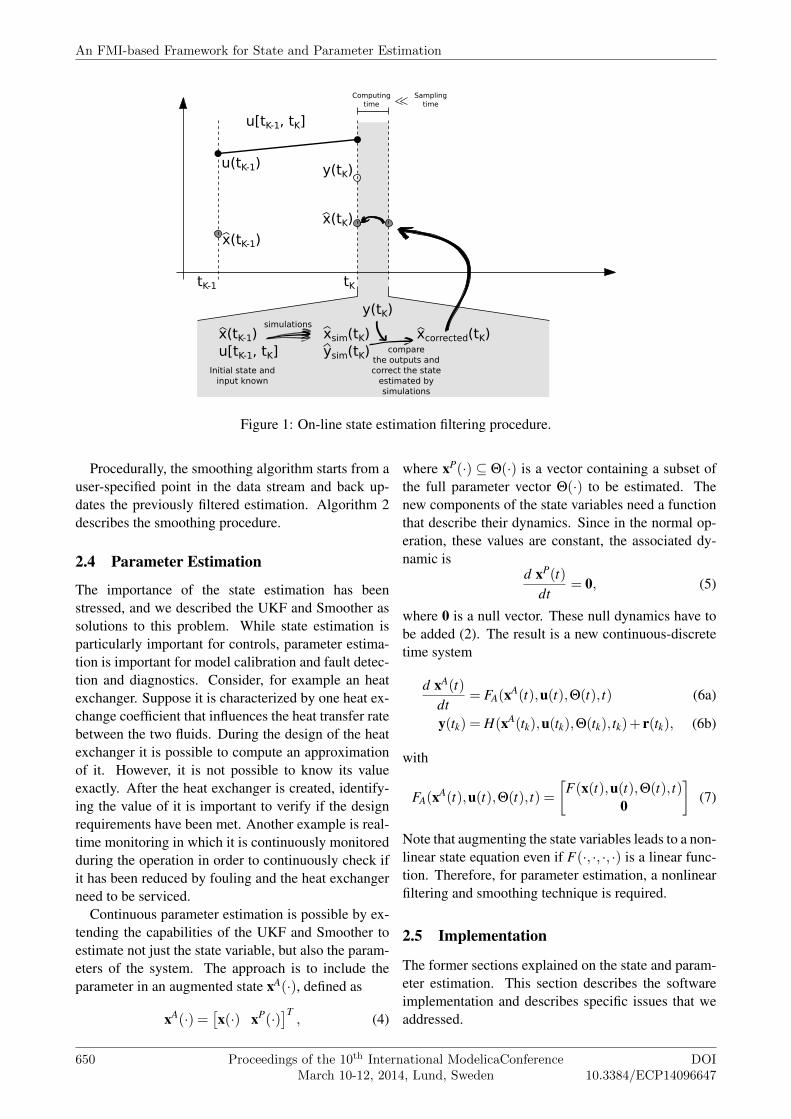
Figure 1 illustrates the filtering process which wewill now explain. At time tk, a measurement of theoutputs y(tk), the inputs and the previous estimationof the state are available. Simulations are performedstarting from the prior knowledge of the state x(tk−1),using the input u(tk−1). Once the results of the simula-tions xsim(tk) and ysim(tk) are available, they are com-pared against the available measurements in order tocorrect the state estimation. The corrected value (i.e.filtered) becomes the actual estimation. Because ofits speed, the estimation can provide near-real-timeupdates, since the time spent for simulating the sys-tem and correcting the estimation is typically shorterthan the sampling time step, in particular for buildingor HVAC applications, where computations take frac-tions of second and sampling intervals are seconds orminutes.

The Algorithm 1 summarize the steps performed bythe UKF. The interested reader can find more informa-tion and details of the actual implementation in [7].

2.3 Smoothing to Improve UKF Estimation

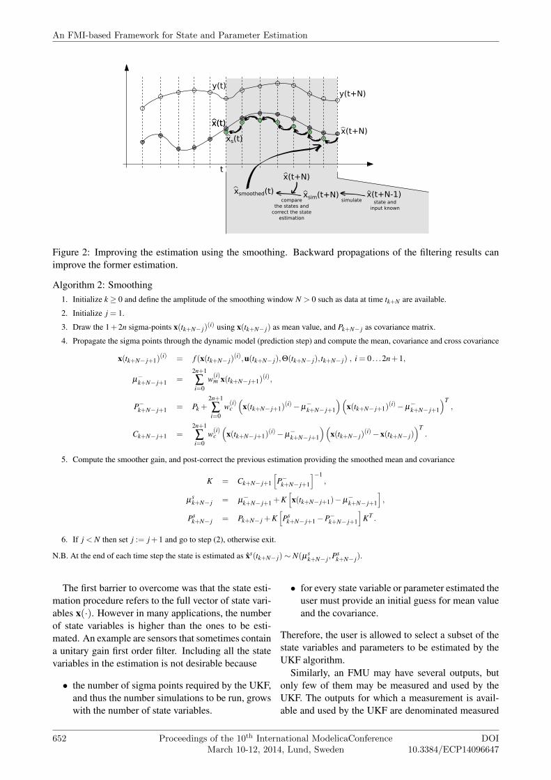
In this subsection, we discuss an additional re-finement procedure to the UKF. The distributionP(x(tk)|y(t1), . . . ,y(tk)) is the probability to ob-serve the state vector x(tk) at time tk given allthe measurements collected. By using more dataP(x(tk)|y(t1), . . . ,y(tk), . . .y(tk+N)), the posterior dis-tribution can be improved through recursive smooth-ing. Hence, the basic idea behind the recursivesmoothing process is to incorporate more measure-ments before providing an estimation of the state. Fig-ure 2 represents the smoothing process. While the fil-ter works forwardly on the data available, and recur-sively provides a state estimation, a smoothing proce-dure back-propagates the information obtained duringthe filtering process, after some amount of data be-comes available, in order to improved the estimationpreviously provided [8].

The smoothing process can be viewed as a delayed,but improved, estimation of the state variables. Thelonger the acceptable delay, the bigger the improve-ment since more information can be used. For exampleif, at a given time, a sensor provides a wrong measure-ment, the filter may not be aware of this and it mayprovide an estimation that does not correspond to thereal value (although the uncertainty bounds will stillbe correct). The smoother observes the trend of the es-timation will reduce this impact of the erroneous data,thus providing an estimation that is less sensitive tomeasurement errors.

Session 4C: Control Applications

DOI10.3384/ECP14096647


649

tK-1 tK

u[tK-1, tK]

y(tK)

Computingtime

x(tK-1)

x(tK-1)u[tK-1, tK]

xsim(tK)ysim(tK)

simulations

y(tK)

comparethe outputs andcorrect the state

estimated by simulations

xcorrected(tK)

x(tK)

Samplingtime

u(tK-1)

Initial state andinput known

Figure 1: On-line state estimation filtering procedure.

Procedurally, the smoothing algorithm starts from auser-specified point in the data stream and back up-dates the previously filtered estimation. Algorithm 2describes the smoothing procedure.

2.4 Parameter Estimation

The importance of the state estimation has beenstressed, and we described the UKF and Smoother assolutions to this problem. While state estimation isparticularly important for controls, parameter estima-tion is important for model calibration and fault detec-tion and diagnostics. Consider, for example an heatexchanger. Suppose it is characterized by one heat ex-change coefficient that influences the heat transfer ratebetween the two fluids. During the design of the heatexchanger it is possible to compute an approximationof it. However, it is not possible to know its valueexactly. After the heat exchanger is created, identify-ing the value of it is important to verify if the designrequirements have been met. Another example is real-time monitoring in which it is continuously monitoredduring the operation in order to continuously check ifit has been reduced by fouling and the heat exchangerneed to be serviced.

Continuous parameter estimation is possible by ex-tending the capabilities of the UKF and Smoother toestimate not just the state variable, but also the param-eters of the system. The approach is to include theparameter in an augmented state xA(·), defined as

xA(·) =[x(·) xP(·)

]T, (4)

where xP(·) ⊆ Θ(·) is a vector containing a subset ofthe full parameter vector Θ(·) to be estimated. Thenew components of the state variables need a functionthat describe their dynamics. Since in the normal op-eration, these values are constant, the associated dy-namic is

d xP(t)dt

= 0, (5)

where 0 is a null vector. These null dynamics have tobe added (2). The result is a new continuous-discretetime system

d xA(t)dt

= FA(xA(t),u(t),Θ(t), t) (6a)

y(tk) = H(xA(tk),u(tk),Θ(tk), tk)+ r(tk), (6b)

with

FA(xA(t),u(t),Θ(t), t) =

[F(x(t),u(t),Θ(t), t)

0

](7)

Note that augmenting the state variables leads to a non-linear state equation even if F(·, ·, ·, ·) is a linear func-tion. Therefore, for parameter estimation, a nonlinearfiltering and smoothing technique is required.

2.5 Implementation

The former sections explained on the state and param-eter estimation. This section describes the softwareimplementation and describes specific issues that weaddressed.



DOI10.3384/ECP14096647

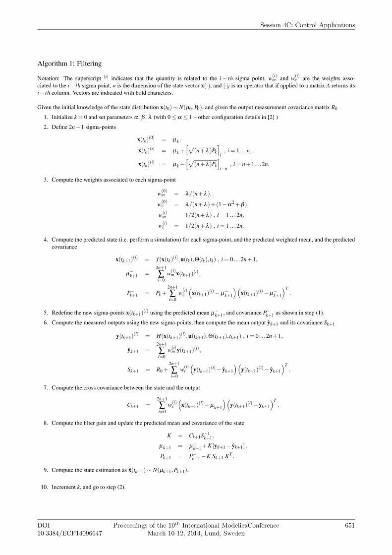
Algorithm 1: Filtering

Notation: The superscript (i) indicates that the quantity is related to the i− th sigma point, w(i)m and w(i)

c are the weights asso-ciated to the i− th sigma point, n is the dimension of the state vector x(·), and [·]i is an operator that if applied to a matrix A returns itsi− th column. Vectors are indicated with bold characters.

Given the initial knowledge of the state distribution x(t0)∼ N(µ0,P0), and given the output measurement covariance matrix R0

1. Initialize k = 0 and set parameters α , β , λ (with 0≤ α ≤ 1 – other configuration details in [2] )

2. Define 2n + 1 sigma-points

x(tk)(0) = µk,

x(tk)(i) = µk +[√

(n + λ )Pk

]i, i = 1 . . .n,

x(tk)(i) = µk−[√

(n + λ )Pk

]i−n

, i = n + 1 . . .2n.

3. Compute the weights associated to each sigma-point

w(0)m = λ/(n + λ ),

w(0)c = λ/(n + λ )+(1−α2 + β ),

w(i)m = 1/2(n + λ ) , i = 1 . . .2n,

w(i)c = 1/2(n + λ ) , i = 1 . . .2n.

4. Compute the predicted state (i.e. perform a simulation) for each sigma-point, and the predicted weighted mean, and the predictedcovariance

x(tk+1)(i) = f (x(tk)(i),u(tk),Θ(tk), tk) , i = 0 . . .2n + 1,

µ−k+1 =2n+1

∑i=0

w(i)m x(tk+1)(i),

P−k+1 = Pk +2n+1

∑i=0

w(i)c

(x(tk+1)(i)−µ−k+1

)(x(tk+1)(i)−µ−k+1

)T.

5. Redefine the new sigma-points x(tk+1)(i) using the predicted mean µ−k+1, and covariance P−k+1 as shown in step (1).

6. Compute the measured outputs using the new sigma-points, then compute the mean output yk+1 and its covariance Sk+1

y(tk+1)(i) = H(x(tk+1)(i),u(tk+1),Θ(tk+1), tk+1) , i = 0 . . .2n + 1,

yk+1 =2n+1

∑i=0

w(i)m y(tk+1)(i),

Sk+1 = R0 +2n+1

∑i=0

w(i)c

(y(tk+1)(i)− yk+1

)(y(tk+1)(i)− yk+1

)T.

7. Compute the cross covariance between the state and the output

Ck+1 =2n+1

∑i=0

w(i)c

(x(tk+1)(i)−µ−k+1

)(y(tk+1)(i)− yk+1

)T.

8. Compute the filter gain and update the predicted mean and covariance of the state

K = Ck+1S−1k+1,

µk+1 = µ−k+1 + K [yk+1− yk+1] ,

Pk+1 = P−k+1−K Sk+1 KT .

9. Compute the state estimation as x(tk+1)∼ N(µk+1,Pk+1).

10. Increment k, and go to step (2).


DOI10.3384/ECP14096647


651

t

y(t)

simulatecomparethe states and

correct the state estimation

state andinput known

x(t+N-1)xsim(t+N)xsmoothed(t)

x(t)x(t+N)

y(t+N)

x(t)

xs(t)

x(t+N)

Figure 2: Improving the estimation using the smoothing. Backward propagations of the filtering results canimprove the former estimation.

Algorithm 2: Smoothing1. Initialize k ≥ 0 and define the amplitude of the smoothing window N > 0 such as data at time tk+N are available.

2. Initialize j = 1.

3. Draw the 1 + 2n sigma-points x(tk+N− j)(i) using x(tk+N− j) as mean value, and Pk+N− j as covariance matrix.

4. Propagate the sigma points through the dynamic model (prediction step) and compute the mean, covariance and cross covariance

x(tk+N− j+1)(i) = f (x(tk+N− j)(i),u(tk+N− j),Θ(tk+N− j), tk+N− j) , i = 0 . . .2n + 1,

µ−k+N− j+1 =2n+1

∑i=0

w(i)m x(tk+N− j+1)(i),

P−k+N− j+1 = Pk +2n+1

∑i=0

w(i)c

(x(tk+N− j+1)(i)−µ−k+N− j+1

)(x(tk+N− j+1)(i)−µ−k+N− j+1

)T,

Ck+N− j+1 =2n+1

∑i=0

w(i)c

(x(tk+N− j+1)(i)−µ−k+N− j+1

)(x(tk+N− j)

(i)−x(tk+N− j))T.

5. Compute the smoother gain, and post-correct the previous estimation providing the smoothed mean and covariance

K = Ck+N− j+1

[P−k+N− j+1

]−1,

µsk+N− j = µ−k+N− j+1 + K

[x(tk+N− j+1)−µ−k+N− j+1

],

Psk+N− j = Pk+N− j + K

[Ps

k+N− j+1−P−k+N− j+1

]KT .

6. If j < N then set j := j + 1 and go to step (2), otherwise exit.

N.B. At the end of each time step the state is estimated as xs(tk+N− j)∼ N(µsk+N− j,P

sk+N− j).

The first barrier to overcome was that the state esti-mation procedure refers to the full vector of state vari-ables x(·). However in many applications, the numberof state variables is higher than the ones to be esti-mated. An example are sensors that sometimes containa unitary gain first order filter. Including all the statevariables in the estimation is not desirable because

• the number of sigma points required by the UKF,and thus the number simulations to be run, growswith the number of state variables.

• for every state variable or parameter estimated theuser must provide an initial guess for mean valueand the covariance.

Therefore, the user is allowed to select a subset of thestate variables and parameters to be estimated by theUKF algorithm.

Similarly, an FMU may have several outputs, butonly few of them may be measured and used by theUKF. The outputs for which a measurement is avail-able and used by the UKF are denominated measured



DOI10.3384/ECP14096647

outputs. The measured outputs requires additional in-formation such the covariance (i.e., the uncertainty as-sociated to the measure) and a time serie containingthe data.

All the inputs and the measured outputs have to beassociated with a time serie. This can be done by as-sociating them with a specific column of a csv file.

Another issue has been encountered regarding therange of validity of states and parameters. For exam-ple, the level of water contained in a tank has to bepositive but not greater than the height of the tank. Weaddressed this issue by constraining the sigma pointswithin user specified upper and lower limits. As de-fault, the min and max values specified in the FMUmodel description file are used.

We also implemented the ability to run the simula-tions in parallel. The computationally demanding partof the UKF and Smoother is the time integration doneusing PyFMI. However this section of the algorithm isentirely parallelizable. By default, our implementationuses one less thread as there are processors to run thesimulation, while a thread manages the simulation andcollects the results. The simulation results generatedby PyFMI can optionally be written to files or not.

All these functionalities have been embedded in fewclasses that use PyFMI. In particular we have defineda new class representing the FMU model in a moregeneral term since the state estimation is a task thatinvolves more than a simple simulation, which is theaim of PyFMI.

2.6 Code snippet

This subsection contains a code snippet that illustrateshow the FMU-based state and parameter estimationframework works. In this example the FMU modelrepresents a mass-spring-damper system, where the in-put is the force F applied to the mass, and the mea-sured output is the mass acceleration a. The two cor-responding data series are stored in a csv file nameddata.csv. The states to be estimated are the position xand its velocity v.# Path o f t h e FMU modelf i l e P a t h = " . / model . fmu "

# I n s t a n t i a t e t h e modelm = Model ( f i l e P a t h , a t o l =1e−5, r t o l =1e−4)

# Path o f t h e CSV f i l e t h a t c o n t a i n s t h e da ta s e r i e sc s v P a t h = " . / d a t a . c sv "

# A s s o c i a t e t h e columns o f t h e c s v f i l e t o t h e i n p u ti n p u t = m. GetInputByName ( "F" )i n p u t . GetCsvReader ( ) . OpenCsv ( c s v P a t h )i n p u t . GetCsvReader ( ) . S e t S e l e c t e d C o l u m n ( " Force " )

# A s s o c i a t e t h e columns o f t h e c s v f i l e t o t h e o u t p u to u t p u t = m. GetOutputByName ( " a " )o u t p u t . GetCsvReader ( ) . OpenCsv ( c s v P a t h )o u t p u t . GetCsvReader ( ) . S e t S e l e c t e d C o l u m n ( " a c c e l e r a t i o n " )

# S p e c i f y t h a t t h i s o u t p u t has t o be compared a g a i n s t# measured da ta c o n t a i n e d i n t h e CSV f i l eo u t p u t . Se tMeasu redOutpu t ( )

# S p e c i f y o u t p u t measurement c o v a r i a n c eo u t p u t . S e t C o v a r i a n c e ( 1 . 0 )

# S p e c i f y t h e s u b s e t o f t h e s t a t e s t o be e s t i m a t e dm. AddVar i ab le (m. G e t V a r i a b l e O b j e c t ( " x " ) )m. AddVar i ab le (m. G e t V a r i a b l e O b j e c t ( " v " ) )

# Get a r e f e r e n c e t o t h e s t a t e s t o be e s t i m a t e dvar_x = m. G e t V a r i a b l e s ( ) [ 0 ]va r_v = m. G e t V a r i a b l e s ( ) [ 1 ]

# S p e c i f y i n i t i a l v a l u e f o r t h e p o s i t i o n# and t h e boundary l i m i t s ( e . g . , p o s i t i o n x must be p o s i t i v e )var_x . S e t I n i t i a l V a l u e ( 2 . 5 )va r_x . S e t C o v a r i a n c e ( 0 . 5 )va r_x . SetMinValue ( 0 . 0 )

# S p e c i f y i n i t i a l v a l u e f o r t h e v e l o c i t yvar_y . S e t I n i t i a l V a l u e ( 0 . 0 )va r_y . S e t C o v a r i a n c e ( 0 . 2 )

# I n i t i a l i z e s i m u l a t o rm. I n i t i a l i z e S i m u l a t o r ( )

# I n s t a n t i a t e UKF and pass t o i t t h e modelUKF = ukfFMU (m)

# Run t h e f i l t e r from 0 . 0 t o 1 0 . 0 s e c o n d st ime , X, Sx , y , Sy = UKF. f i l t e r ( s t a r t = 0 . 0 , s t o p = 1 0 . 0 )

# p l o t t i n g . . .

This framework reduces the effort to set up a stateor parameter estimation. The model can be created inModelica and directly imported as an FMU, avoidingthe user to rewrite the model in the right format re-quired by the UKF. Other functionalities provide aneasy way to specify the state variables or parameter tobe estimated, together with the data series to be usedas inputs and outputs.

3 Application: FDD

This section contains an example that shows how theFMU-based state and parameter estimation algorithmcan be used for fault detection and diagnosis.

FDD algorithms based on state estimation tech-niques are known to be more suitable than other ap-proaches based on neural networks or principal com-ponent analysis for detecting multiple faults [9, 10,11], they can compute the fault probabilities and theyprovide an indication of what is not working as ex-pected in the system. All these features are possiblethank to the probabilistic description of the state vari-ables and parameters the estimation techniques pro-vide.

A drawback of state estimation based strategies isthat they require a slightly higher modeling effort, e.g.,to include explicit fault descriptions in the model it-self. However, various open-source modeling tools(e.g. OpenModelica and JModelica), and modeling li-braries for buildings (Modelica Buildings library [12])are available, and they provide two main advantages:reducing the effort required to set up the model, and


DOI10.3384/ECP14096647


653

TdP

F

uu: opening commandT: temperature sensorF: flow sensordP: differential pressure sensor

Figure 3: Schematic of the system.

reducing the risk of modeling errors since they are typ-ically validated and tested.

The availability of these tools and libraries togetherwith the FMU-based state and parameter estimation al-gorithm put in place a framework for creating with alow level of effort a model-based FDD algorithm.

The considered system is a valve that regulates thewater flow rate in a water distribution system (see Fig-ure 3). The system is described by the following equa-tions

m(t) = φ(x(t))Av√

ρ(t)√

∆p(t), (8a)

x(t)+ τ x(t) = u(t), (8b)

where m(·) is the mass flow rate passing through thevalve, ∆p(·) is the pressure difference across it, u(·)is the valve opening command signal, x(·) is the valveopening position, τ is the actuator time constant, φ(·)is the power-law opening characteristic, Av is the flowcoefficient and ρ(·) is the fluid density (please notethat the square root of the pressure difference is reg-ularized around zero flow in order to prevent singu-larities in the solution). The system has three sensors(see Figure 3) that respectively measure the pressuredifference across the valve, the water temperature T (·)and the mass flow rate passing through it. All the sen-sors are affected by measurement noise. In addition,the mass flow rate sensor is also affected by a thermaldrift.

T N(t) = T (t)+ ηT (t) (9a)

∆pN(t) = ∆p(t)+ ηP(t) (9b)

mN+D(t) = (1 + λ (T (t)−Tre f ))m(t)+ ηm(t) (9c)

The measurement equations are described in (9),where the superscript N indicates a measurement af-fected by noise, the superscript N+D indicates the pres-ence of both noise and thermal drift, Tre f is the refer-ence temperature at which the sensor has no drift, λis the thermal drift coefficient and ηT (·), ηP(·), andηm(·) are three uniform white noises affecting respec-tively the temperature, pressure and mass flow rate

Figure 4: Input signals of the faulty valve model: wa-ter temperature (blue) and pressure difference (green).The lines represent the data generated by simulation,while the dots represent the sampled and noisy versionprovided to the UKF.

measurements. These signals are sampled every twoseconds.

Suppose during the operation, at t = 80 s, the valvebecomes faulty. The fault affects the ability of thevalve to control its opening position. The valve open-ing cannot go below 20% (causing a leakage) and over60% (it gets stuck). At t = 250 s, the valve stuck posi-tion moves from 60% to 90%.

The fault identification procedure is asked to iden-tify whether the valve not works as expected, that isits opening position follows the command signal. Thefault identification is performed using the UKF thatuses as input signals for its model the noisy pressuredifference (see Figure 4), the noisy water temperature(see Figure 4) and the command signal (see Figure 6).The command signal is noise free because it is com-puted by some external controller and not measured.The UKF compares the output of its simulations withthe measured mass flow rate (see Figure 5) that is af-fected by both noise and thermal drift. The effect ofthe thermal drift is visible in Figure 5 where the greendots represent the measured mass flow rate while thegreen line is the actual mass flow rate passing throughthe valve.

The UKF and the smother estimate the value of thestate variable x(t) representing the valve opening posi-tion and the parameter λ , the thermal drift coefficient.The length of the augmented state is n = 2. Hence forevery estimation step, the UKF performs 1+2×2 = 5simulations. The UKF has the initial conditions x(0)∼N(0.8,0.05) and λ ∼N(0,0.7 ·10−3), the output noise



DOI10.3384/ECP14096647

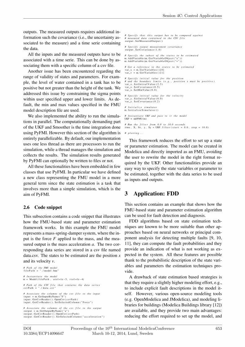
Figure 5: The green line represent the mass flow ratethat is passing through the valve. The green dots arethe measurements of the mass flow rate (affected bynoise and sensor thermal drift) used by the UKF. Thered line is the UKF estimation, while the blue line isthe smoother estimation.

covariance matrix is R = [0.05], and the filter coeffi-cients are α = 1√

3, β = 2 and k = 3−n = 1.

As shown in Figure 5, the measured mass flow rate(green dots) are far from the real mass flow rate (greenline). Despite the measurement error, the UKF andthe smoother provide an estimation with a good accu-racy (red and blue lines in Figure 5). The mass flowrates computed by the UKF, ˆm, and the smoother, ˆmS,are close to the real one, m, because they are able toestimate both the valve opening position and the sen-sor drift coefficient, as shown in Figures 6 and 7. Asexpected the smoother is able to provide a better esti-mation since it uses more data. The time spent by theUKF to perform the simulations and computing the es-timations was about 0.05 s, that is lower than the sam-pling time of 2 s. The speed of this UKF based FDDalgorithm allows a real-time implementation for thisparticular application.

4 General Applicability

The UKF and in general state/parameter estimationtechniques are well known solutions used in manyfields. We presented an approach that reduces the ef-fort needed to set up a state and parameter estimationfor models created with simulation programs that areFMI compliant. The example shows how this tool canbe used for FDD purposes in the context of HVAC sys-tems. However, this tool can be used in other con-

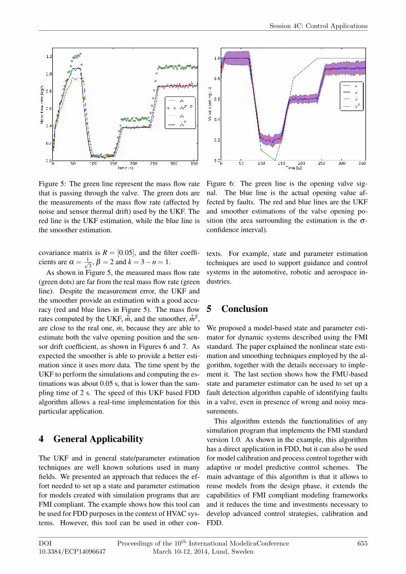
Figure 6: The green line is the opening valve sig-nal. The blue line is the actual opening value af-fected by faults. The red and blue lines are the UKFand smoother estimations of the valve opening po-sition (the area surrounding the estimation is the σ -confidence interval).

texts. For example, state and parameter estimationtechniques are used to support guidance and controlsystems in the automotive, robotic and aerospace in-dustries.

5 Conclusion

We proposed a model-based state and parameter esti-mator for dynamic systems described using the FMIstandard. The paper explained the nonlinear state esti-mation and smoothing techniques employed by the al-gorithm, together with the details necessary to imple-ment it. The last section shows how the FMU-basedstate and parameter estimator can be used to set up afault detection algorithm capable of identifying faultsin a valve, even in presence of wrong and noisy mea-surements.

This algorithm extends the functionalities of anysimulation program that implements the FMI standardversion 1.0. As shown in the example, this algorithmhas a direct application in FDD, but it can also be usedfor model calibration and process control together withadaptive or model predictive control schemes. Themain advantage of this algorithm is that it allows toreuse models from the design phase, it extends thecapabilities of FMI compliant modeling frameworksand it reduces the time and investments necessary todevelop advanced control strategies, calibration andFDD.


DOI10.3384/ECP14096647


655

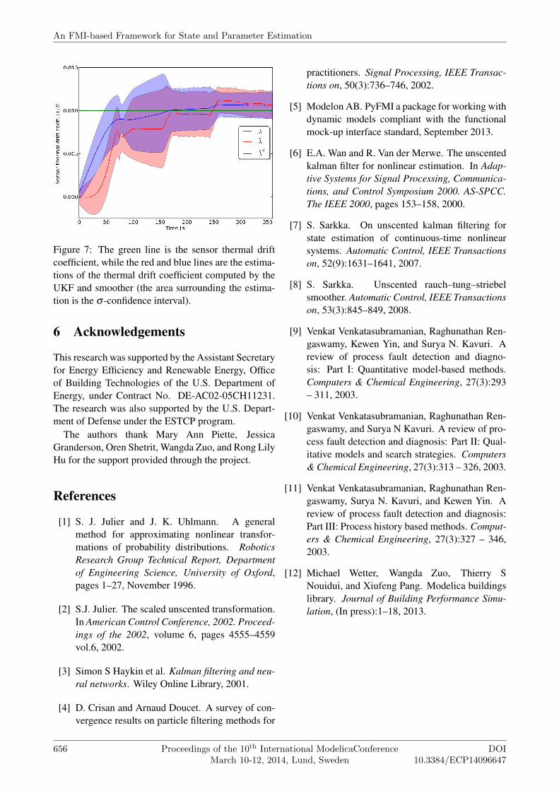
Figure 7: The green line is the sensor thermal driftcoefficient, while the red and blue lines are the estima-tions of the thermal drift coefficient computed by theUKF and smoother (the area surrounding the estima-tion is the σ -confidence interval).

6 Acknowledgements

This research was supported by the Assistant Secretaryfor Energy Efficiency and Renewable Energy, Officeof Building Technologies of the U.S. Department ofEnergy, under Contract No. DE-AC02-05CH11231.The research was also supported by the U.S. Depart-ment of Defense under the ESTCP program.

The authors thank Mary Ann Piette, JessicaGranderson, Oren Shetrit, Wangda Zuo, and Rong LilyHu for the support provided through the project.

References

[1] S. J. Julier and J. K. Uhlmann. A generalmethod for approximating nonlinear transfor-mations of probability distributions. RoboticsResearch Group Technical Report, Departmentof Engineering Science, University of Oxford,pages 1–27, November 1996.

[2] S.J. Julier. The scaled unscented transformation.In American Control Conference, 2002. Proceed-ings of the 2002, volume 6, pages 4555–4559vol.6, 2002.

[3] Simon S Haykin et al. Kalman filtering and neu-ral networks. Wiley Online Library, 2001.

[4] D. Crisan and Arnaud Doucet. A survey of con-vergence results on particle filtering methods for

practitioners. Signal Processing, IEEE Transac-tions on, 50(3):736–746, 2002.

[5] Modelon AB. PyFMI a package for working withdynamic models compliant with the functionalmock-up interface standard, September 2013.

[6] E.A. Wan and R. Van der Merwe. The unscentedkalman filter for nonlinear estimation. In Adap-tive Systems for Signal Processing, Communica-tions, and Control Symposium 2000. AS-SPCC.The IEEE 2000, pages 153–158, 2000.

[7] S. Sarkka. On unscented kalman filtering forstate estimation of continuous-time nonlinearsystems. Automatic Control, IEEE Transactionson, 52(9):1631–1641, 2007.

[8] S. Sarkka. Unscented rauch–tung–striebelsmoother. Automatic Control, IEEE Transactionson, 53(3):845–849, 2008.

[9] Venkat Venkatasubramanian, Raghunathan Ren-gaswamy, Kewen Yin, and Surya N. Kavuri. Areview of process fault detection and diagno-sis: Part I: Quantitative model-based methods.Computers & Chemical Engineering, 27(3):293– 311, 2003.

[10] Venkat Venkatasubramanian, Raghunathan Ren-gaswamy, and Surya N Kavuri. A review of pro-cess fault detection and diagnosis: Part II: Qual-itative models and search strategies. Computers& Chemical Engineering, 27(3):313 – 326, 2003.

[11] Venkat Venkatasubramanian, Raghunathan Ren-gaswamy, Surya N. Kavuri, and Kewen Yin. Areview of process fault detection and diagnosis:Part III: Process history based methods. Comput-ers & Chemical Engineering, 27(3):327 – 346,2003.

[12] Michael Wetter, Wangda Zuo, Thierry SNouidui, and Xiufeng Pang. Modelica buildingslibrary. Journal of Building Performance Simu-lation, (In press):1–18, 2013.



DOI10.3384/ECP14096647

Date post:	20-Sep-2018
Category:	Documents
Upload:	votram
View:	217 times
Download:	0 times

An FMI-based Framework for State and Parameter...

Documents