45
An Illustrative Example
| Date post: | 21-Dec-2015 |
| Category: |
Documents |
| View: | 431 times |
| Download: | 6 times |
AnIllustrativeExample
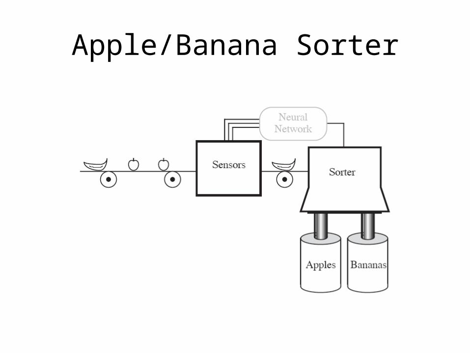
Apple/Banana Sorter
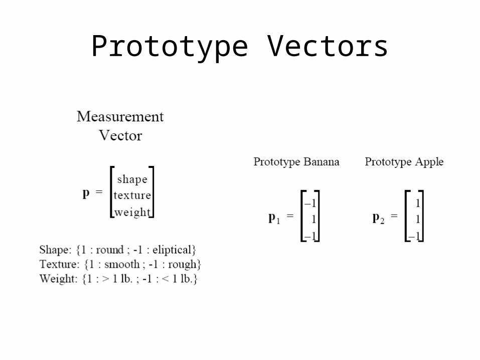
Prototype Vectors
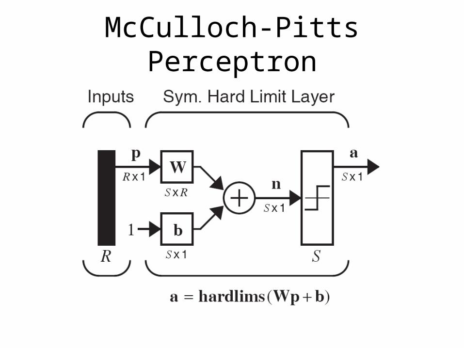
McCulloch-Pitts Perceptron
Perceptron Training
• How can we train a perceptron for a classification task?
• We try to find suitable values for the weights in such a way that the training examples are correctly classified.
• Geometrically, we try to find a hyper-plane that separates the examples of the two classes.
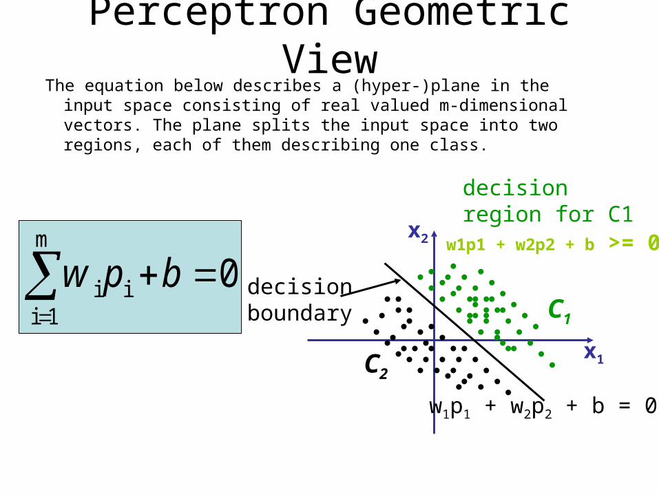
Perceptron Geometric ViewThe equation below describes a (hyper-)plane in the input space
consisting of real valued m-dimensional vectors. The plane splits the input space into two regions, each of them describing one class.
m
i ii 1
0w p b
x2
C1
C2x1
decisionboundary
w1p1 + w2p2 + b = 0
decisionregion for C1
w1p1 + w2p2 + b >= 0
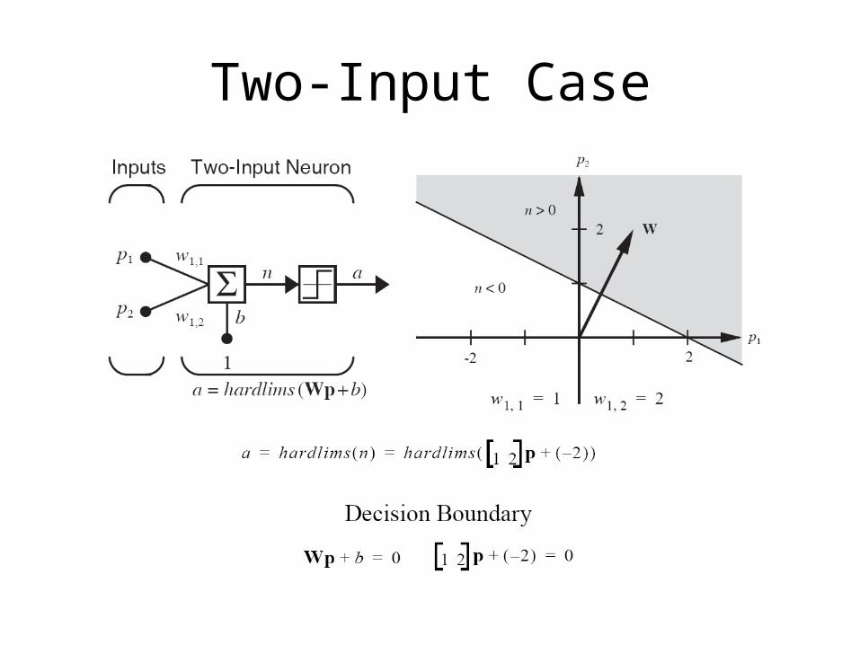
Two-Input Case
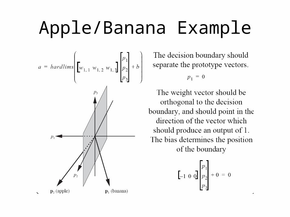
Apple/Banana Example
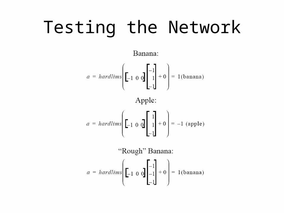
Testing the Network
XOR problem
x1 x2 x1 x2
-1 -1 -1 -1 1 1 1 -1 1 1 1 -1
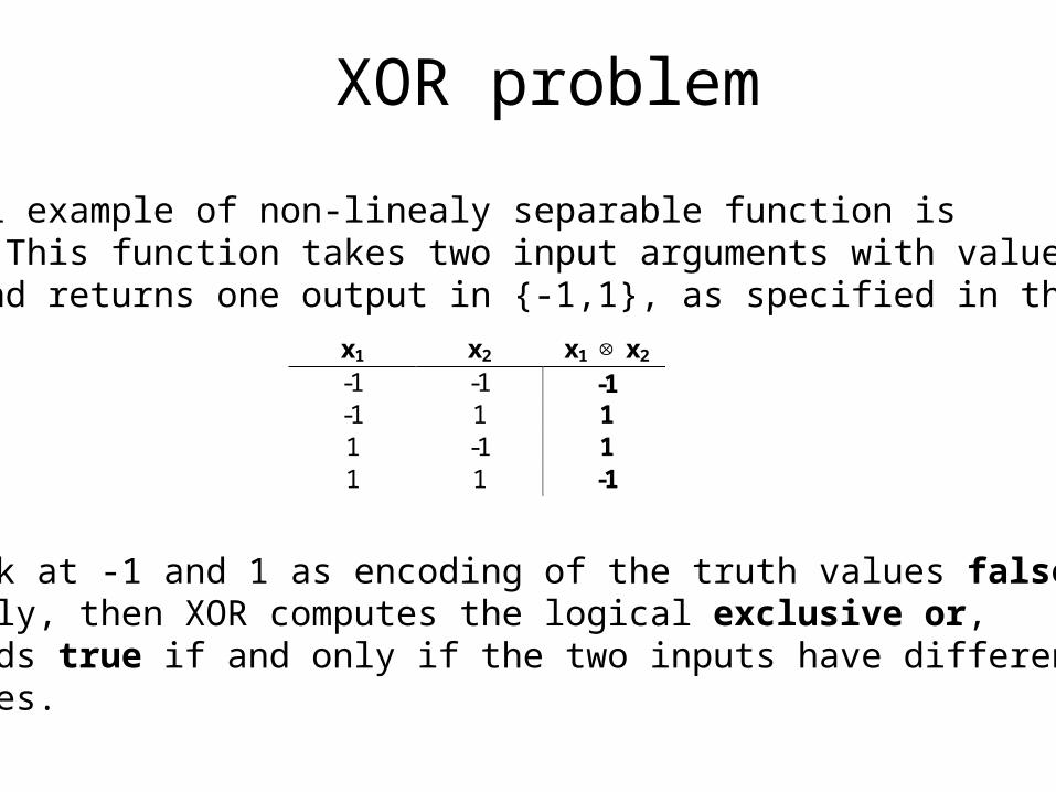
A typical example of non-linealy separable function isthe XOR. This function takes two input arguments with values in {-1,1} and returns one output in {-1,1}, as specified in the followingtable:
If we think at -1 and 1 as encoding of the truth values false and true, respectively, then XOR computes the logical exclusive or,which yields true if and only if the two inputs have different truth values.
XOR problem
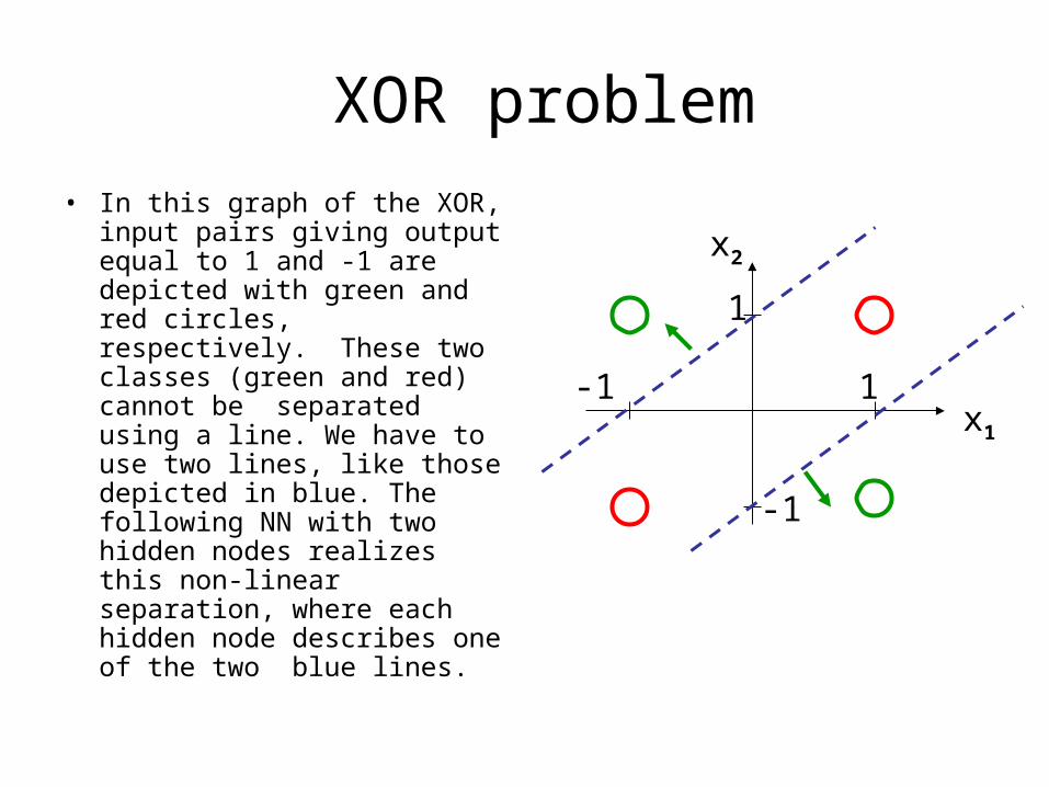
• In this graph of the XOR, input pairs giving output equal to 1 and -1 are depicted with green and red circles, respectively. These two classes (green and red) cannot be separated using a line. We have to use two lines, like those depicted in blue. The following NN with two hidden nodes realizes this non-linear separation, where each hidden node describes one of the two blue lines.
1
1
-1
-1
x2
x1
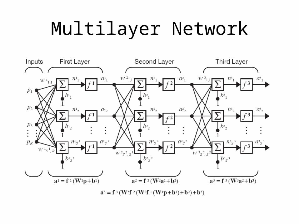
Multilayer Network
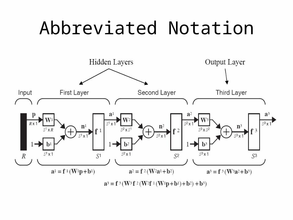
Abbreviated Notation
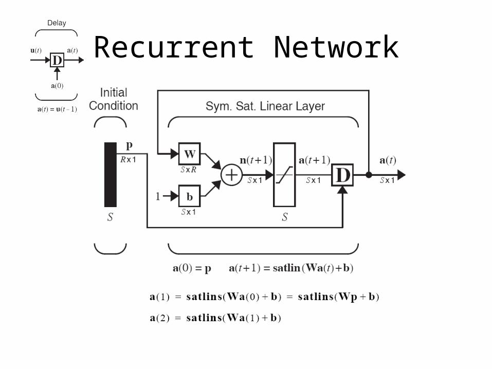
Recurrent Network
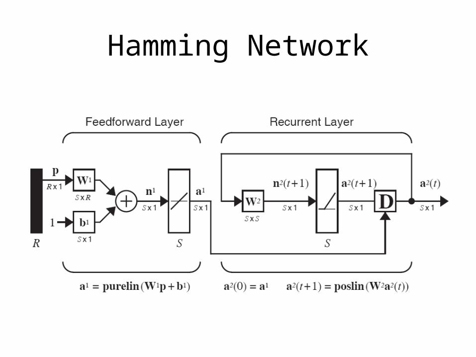
Hamming Network
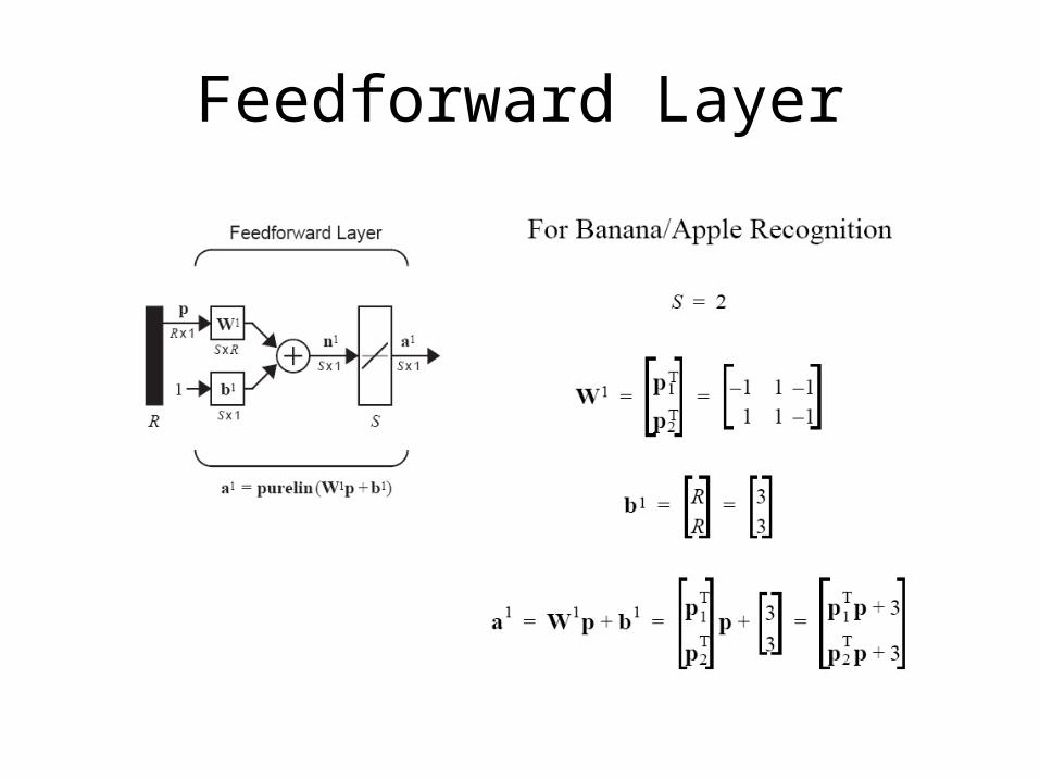
Feedforward Layer
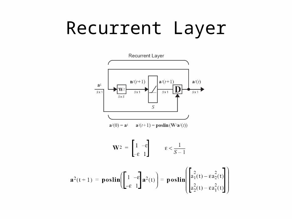
Recurrent Layer
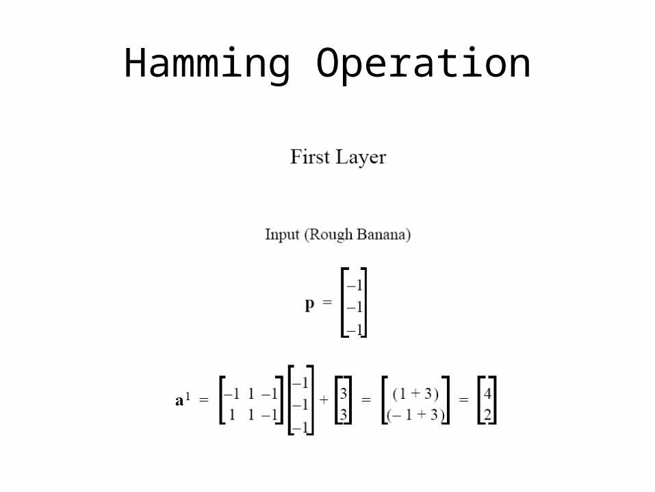
Hamming Operation
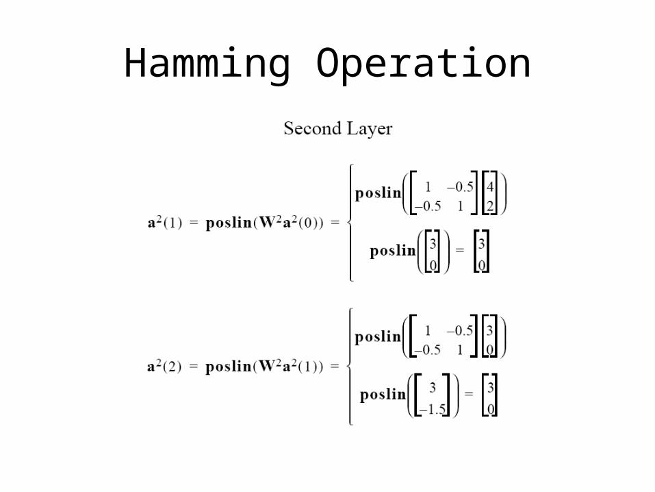
Hamming Operation
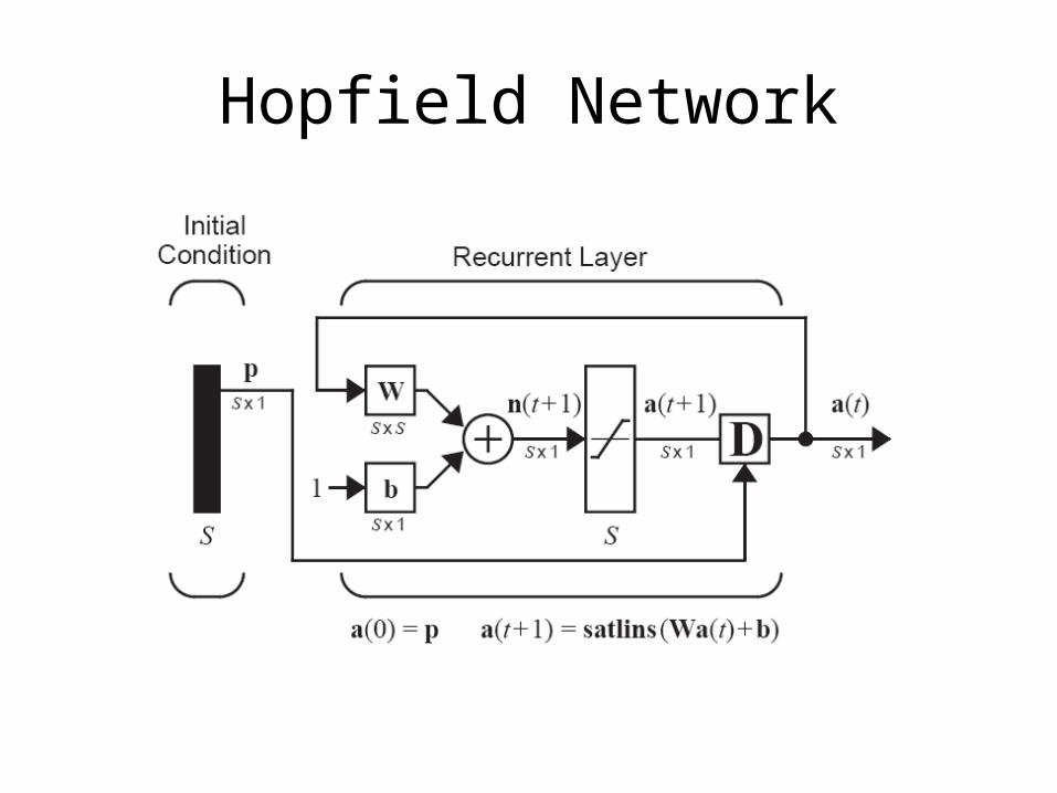
Hopfield Network
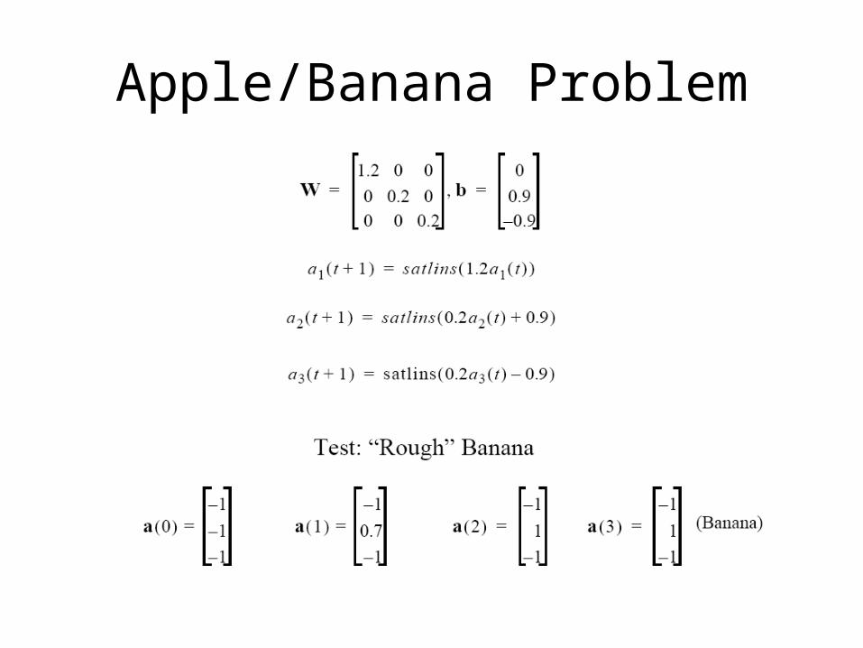
Apple/Banana Problem
Summary
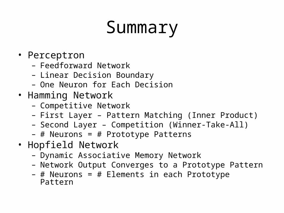
• Perceptron– Feedforward Network– Linear Decision Boundary– One Neuron for Each Decision
• Hamming Network– Competitive Network– First Layer – Pattern Matching (Inner Product)– Second Layer – Competition (Winner-Take-All)– # Neurons = # Prototype Patterns
• Hopfield Network– Dynamic Associative Memory Network– Network Output Converges to a Prototype Pattern– # Neurons = # Elements in each Prototype Pattern
Learning Rules
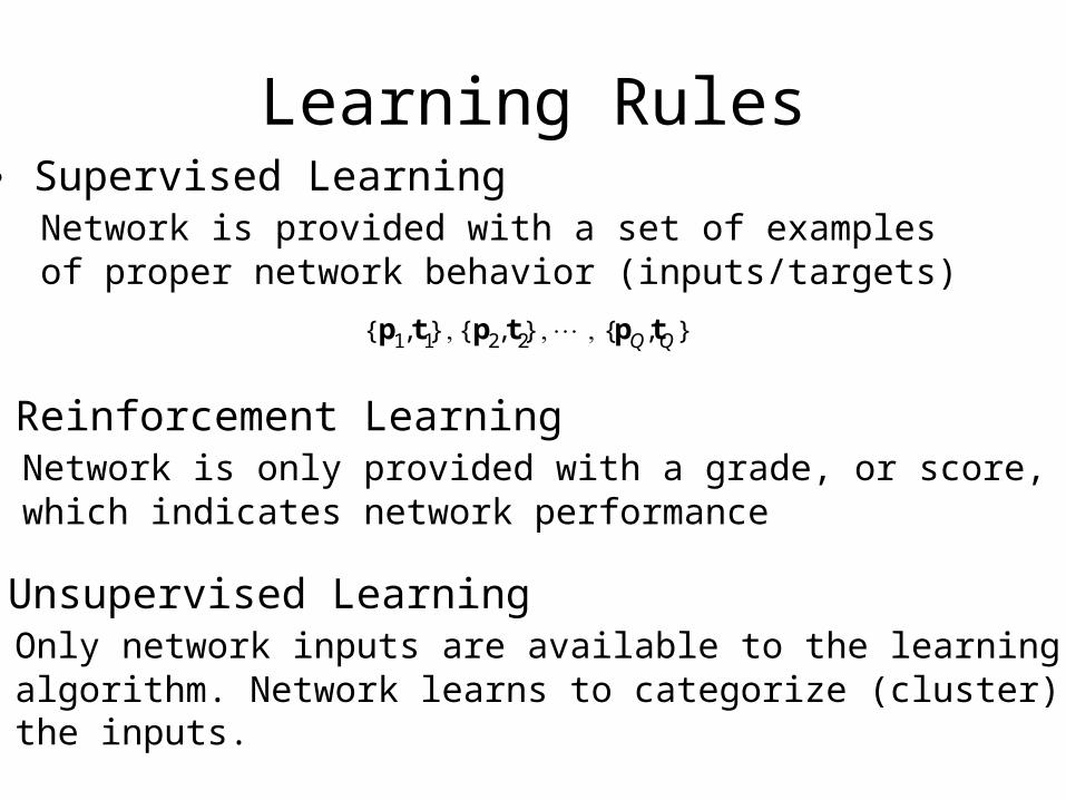
p1 t1{ , } p2 t2{ , } pQ tQ{ , }
• Supervised LearningNetwork is provided with a set of examplesof proper network behavior (inputs/targets)
• Reinforcement LearningNetwork is only provided with a grade, or score,which indicates network performance
• Unsupervised LearningOnly network inputs are available to the learningalgorithm. Network learns to categorize (cluster)the inputs.
Early Learning Rules
• These learning rules are designed for single layer neural networks
• They are generally more limited in their applicability.
• Some of the early algorithms are:– Perceptron learning– LMS learning– Grossberg learning
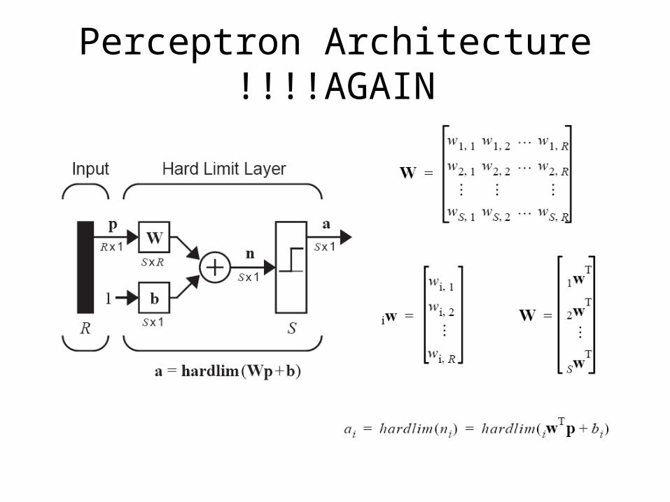
Perceptron Architecture AGAIN!!!!

Single-Neuron Perceptron
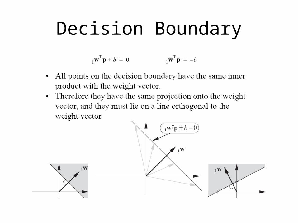
Decision Boundary
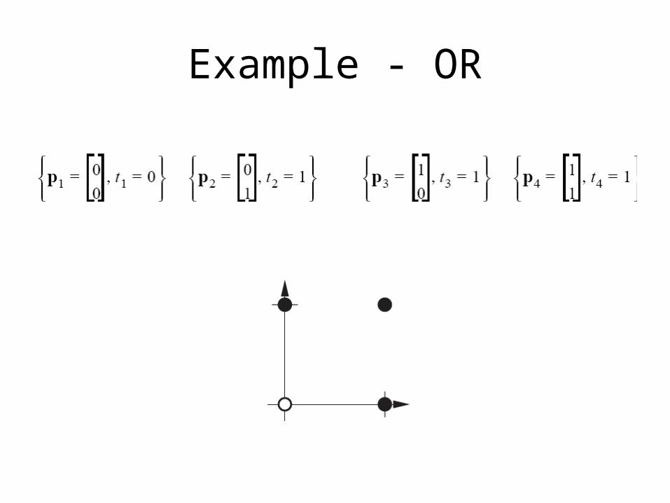
Example - OR

OR Solution
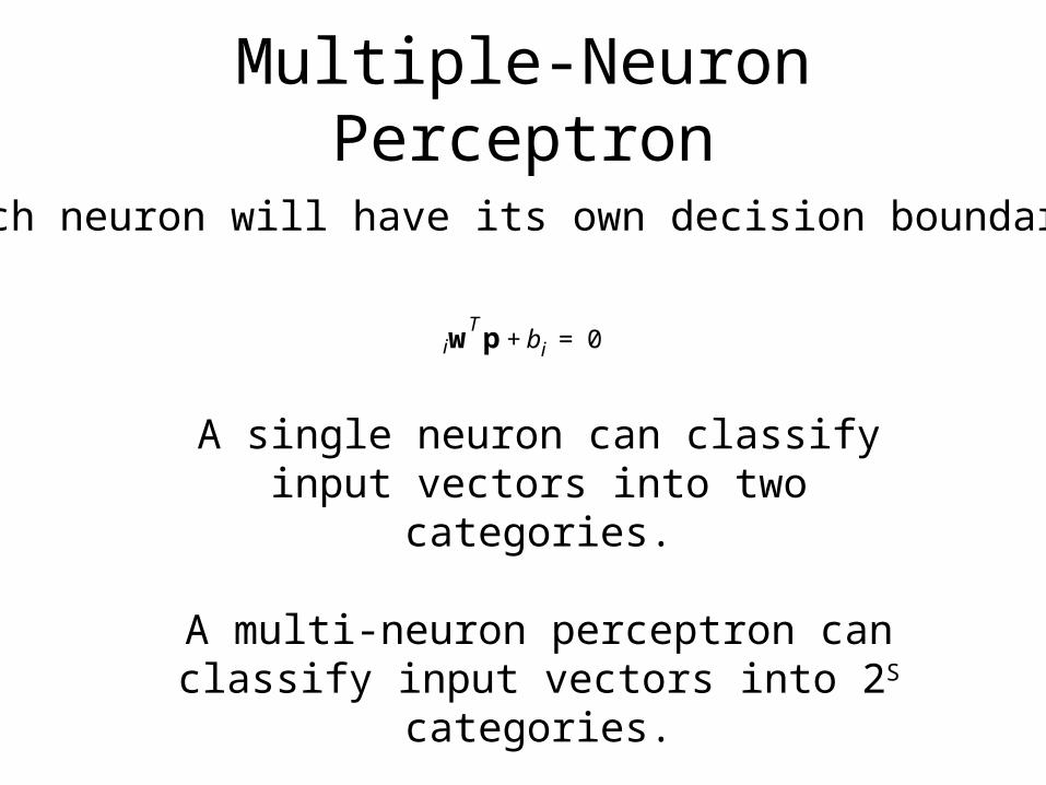
Multiple-Neuron Perceptron
Each neuron will have its own decision boundary.
wT
i p bi+ 0=
A single neuron can classify input vectors into two categories.
A multi-neuron perceptron can classify input vectors into 2S categories.
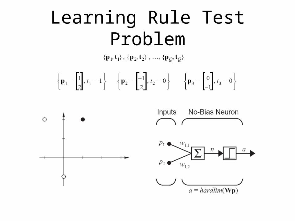
Learning Rule Test Problem
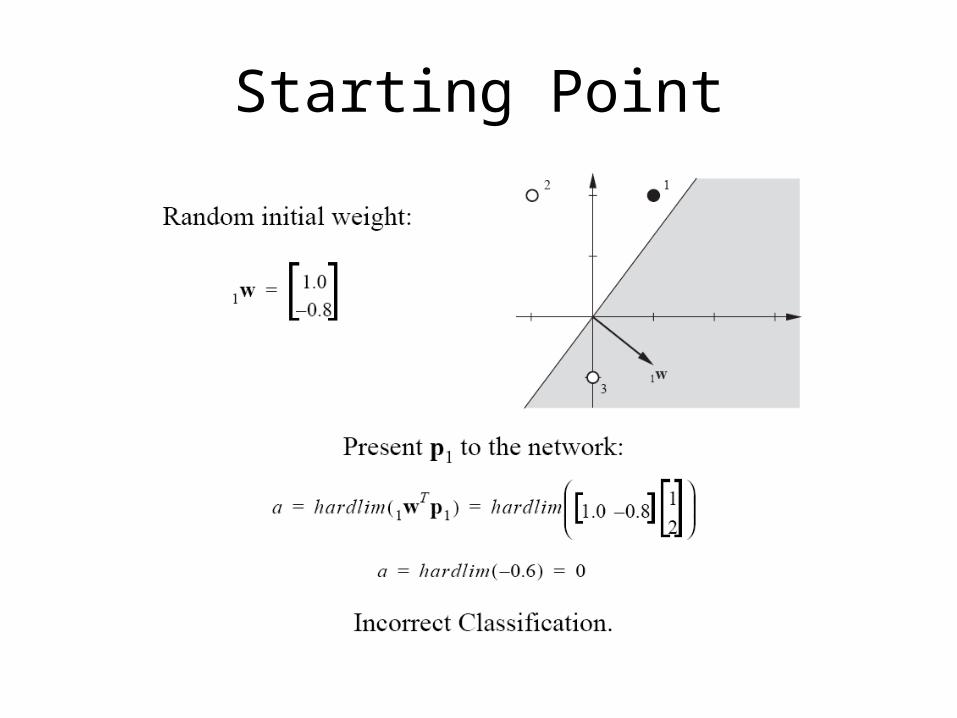
Starting Point
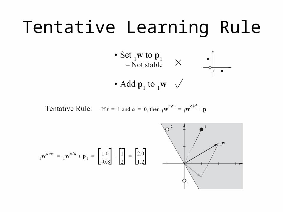
Tentative Learning Rule
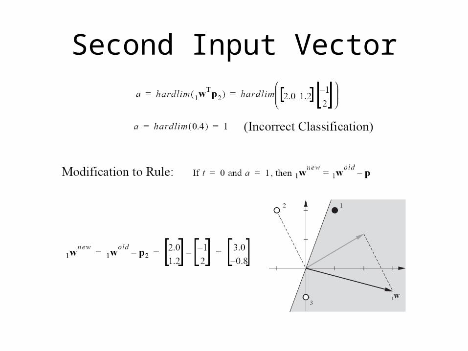
Second Input Vector
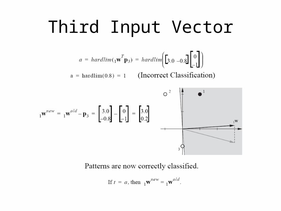
Third Input Vector
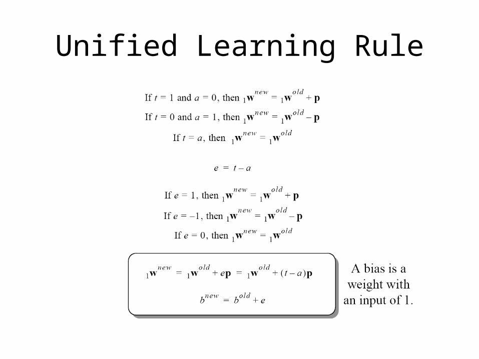
Unified Learning Rule
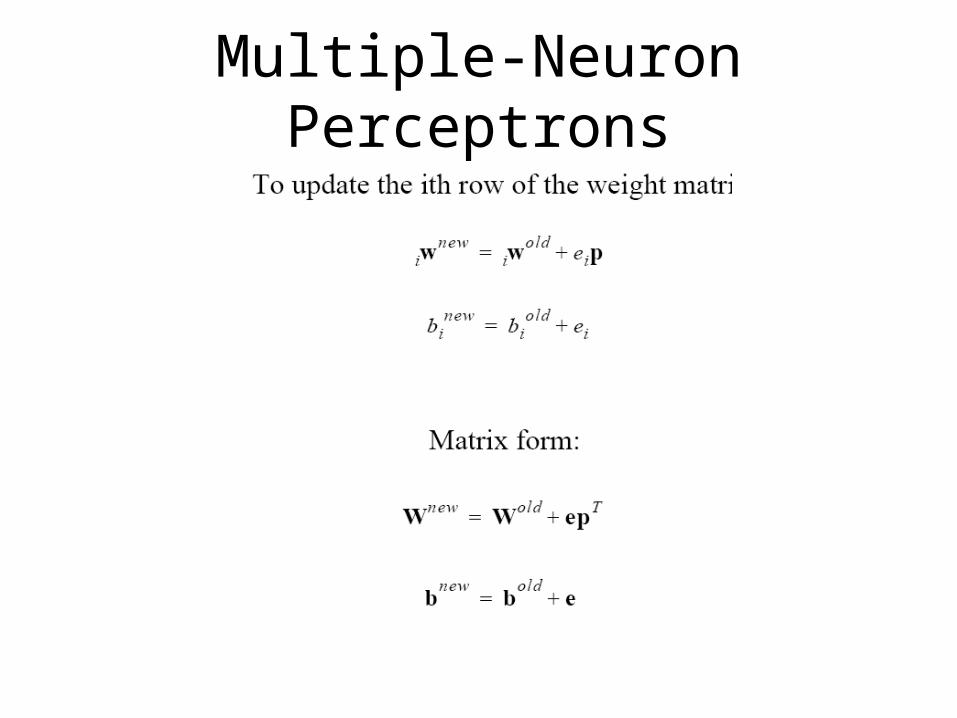
Multiple-Neuron Perceptrons
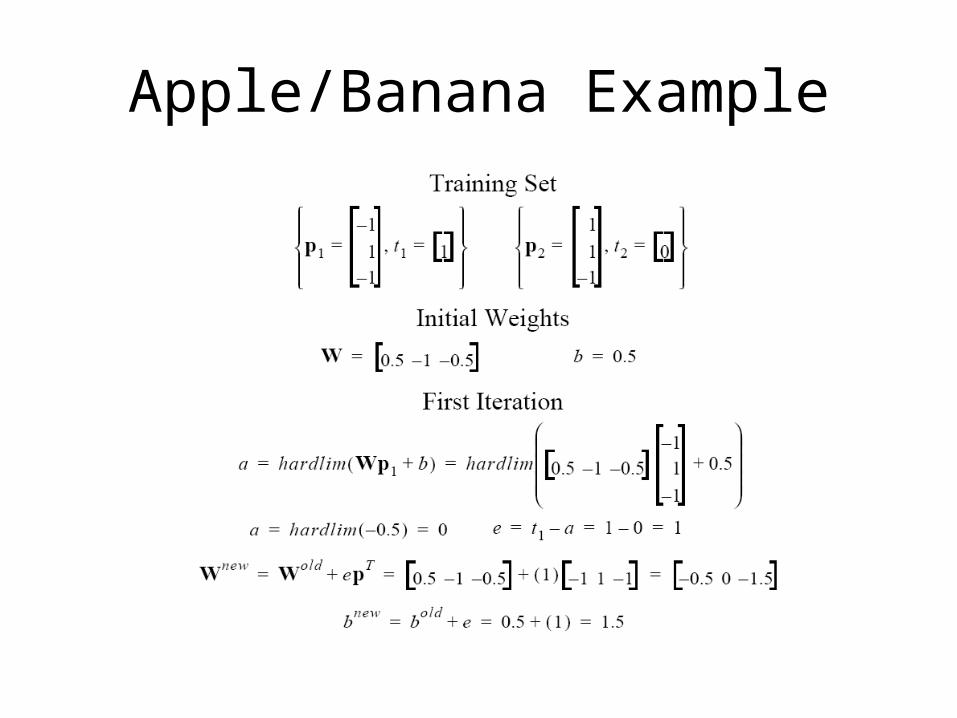
Apple/Banana Example
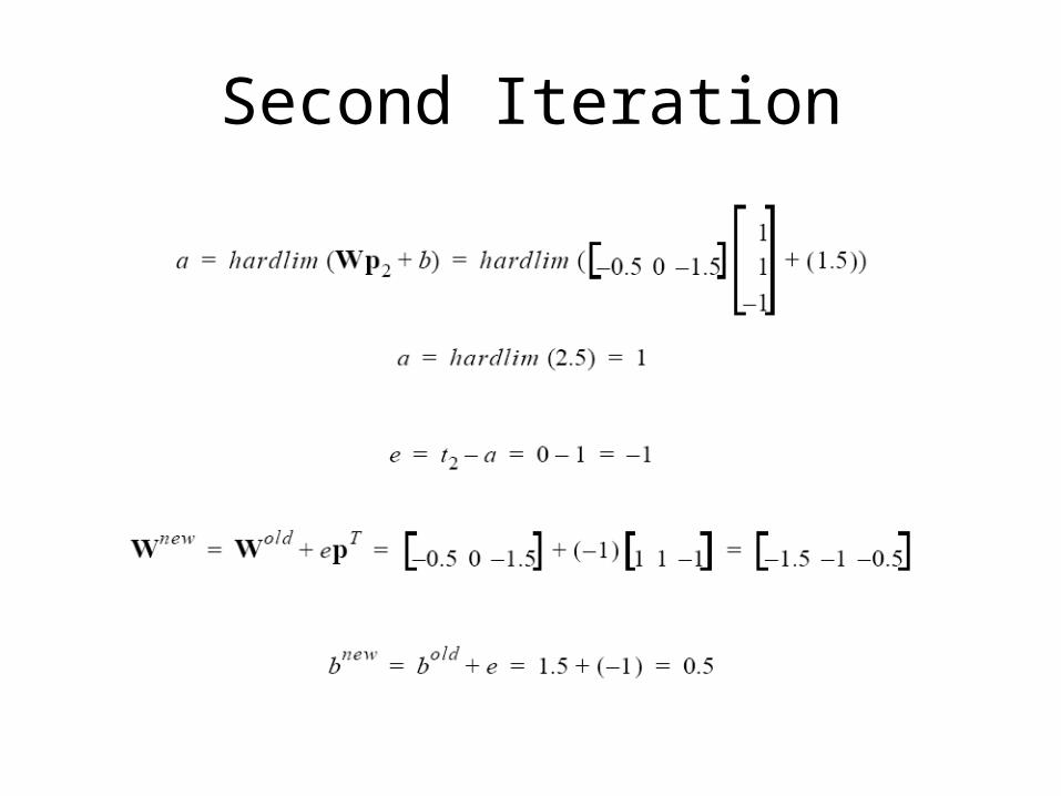
Second Iteration
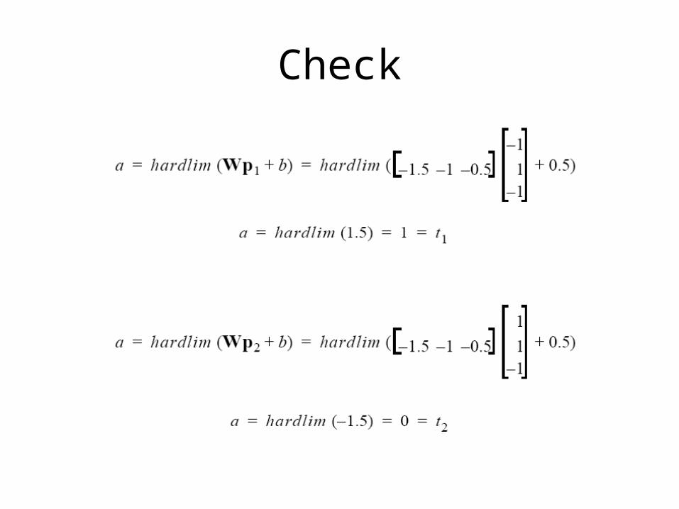
Check
Perceptron Rule Capability
The perceptron rule will always converge to weights which accomplish the desired classification, assuming that
such weights exist.
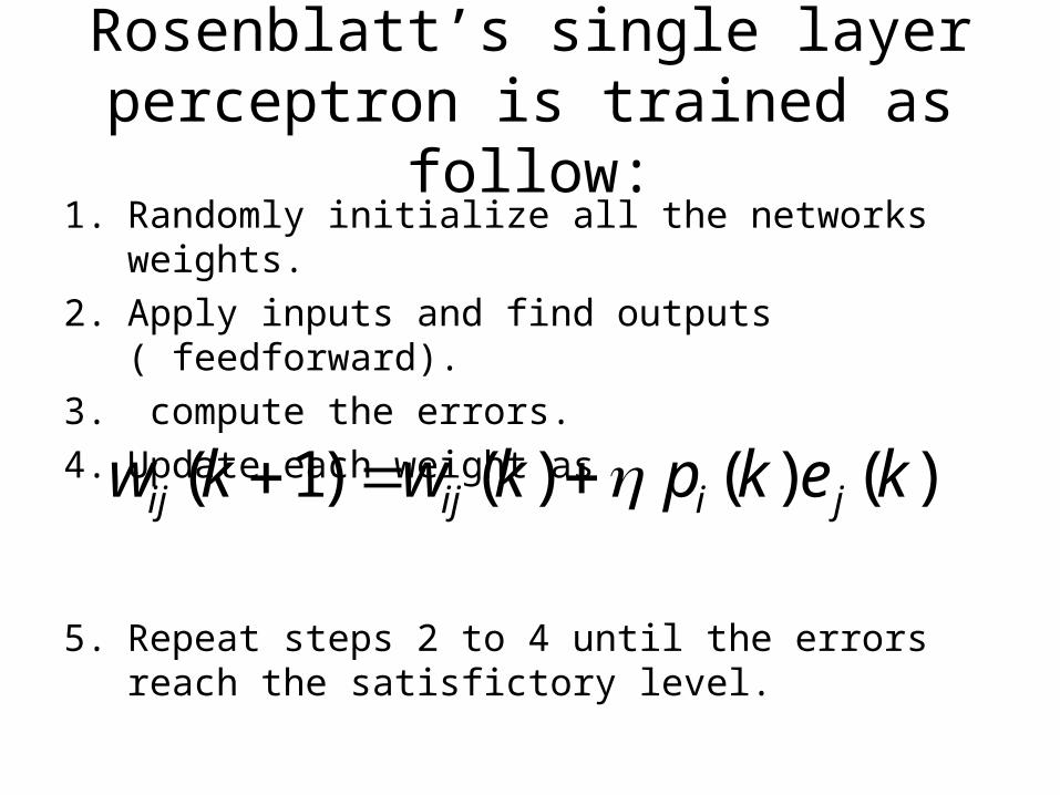
Rosenblatt’s single layer perceptron is trained as follow:
1. Randomly initialize all the networks weights.
2. Apply inputs and find outputs ( feedforward).
3. compute the errors.
4. Update each weight as
5. Repeat steps 2 to 4 until the errors reach the satisfictory level.
)()()()1( kekpkwkw jiijij

What is this:
• Name : Learning rate.• Where is living: usually between 0 and 1.• It can change it’s value during learning.• Can define separately for each parameters.
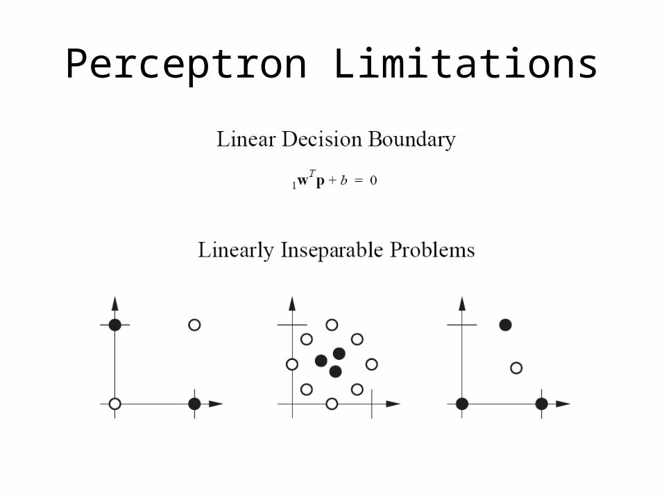
Perceptron Limitations

You Can Find Your First Homework here
http://saba.kntu.ac.ir/eecd/People/aliyari/
NEXT WEEK


