energies

Article

An Improved Bare Bone Multi-Objective ParticleSwarm Optimization Algorithm for Solar ThermalPower Plants

Qun Niu 1,*, Han Wang 1, Ziyuan Sun 1 and Zhile Yang 2

1 School of Mechanical Engineering and Automation, Shanghai Key Laboratory of Power StationAutomation Technology, Shanghai University, Shanghai 200444, China

2 Shenzhen Institute of Advanced Technology, Chinese Academy of Sciences, Shenzhen 518055, China* Correspondence: nq@shu.edu.cn

Received: 16 October 2019; Accepted: 17 November 2019; Published: 25 November 2019 �����������������

Abstract: Solar energy has many advantages, such as being abundant, clean and environmentallyfriendly. Solar power generation has been widely deployed worldwide as an important form ofrenewable energy. The solar thermal power generation is one of a few popular forms to utilizesolar energy, yet its modelling is a complicated problem. In this paper, an improved bare bonemulti-objective particle swarm optimization algorithm (IBBMOPSO) is proposed based on the barebone multi-objective particle swarm optimization algorithm (BBMOPSO). The algorithm is first testedon a set of benchmark problems, confirming its efficacy and the convergency speed. Then, it isapplied to optimize two typical solar power generation systems including the solar Stirling powergeneration and the solar Brayton power generation; the results show that the proposed algorithmoutperforms other algorithms for multi-objective optimization problems.

Keywords: solar Stirling power system; solar Brayton power system; particle swarm optimization(PSO); multi-objective optimization problems (MOP)

1. Introduction

The energy issue is viewed as one of many global problems in the 21st century and it is projectedthat the global energy demand will increase by almost a quarter by 2040 [1]. The continuous rise ofprices for fossil fuels and the climate change due to substantive consumption of non-renewable energieshave caused the shift of energy landscape, from the way the energy is sourced to the way energyis consumed. The landscape change of the energy mix is also largely due to more strict legislationson pollutant and green-gas-house emissions and policies to encourage the use of renewable sources.For example, the European Union requires all its members to take a series of measures to improveenergy efficiency of at least 20% [2]. In addition to this initiative, the United Nations General Assemblydeclared the decade 2014–2024 as the “Decade of Sustainable Energy for All”, given the importance ofenergy issues for sustainable development [3] and encouraging and supporting the extended use ofrenewable energy resources (RES).

As an ideal renewable energy source, solar energy is one of the most abundant energy resources.Solar power has many advantages such as being clean, renewable, and easy to store [4]. Solarpower can be used to generate electricity wherever there is sunshine. Therefore, in the context ofthe growing global energy demand and increasing concerns relating to resources, environment andclimate, governments worldwide have developed a range of policies and incentive mechanisms topromote the development and roll-out of renewable generation technologies for solar and wind energysources [5].

Energies 2019, 12, 4480; doi:10.3390/en12234480 www.mdpi.com/journal/energies

Energies 2019, 12, 4480 2 of 22

Solar thermal power generation technology is a relatively mature technology which mainlyuses the solar concentrating system to convert the solar energy to a high temperature steam andthen drives the generators to generate electricity [6]. Representative solar thermal power generationsystems include a solar Stirling cycle power generation system and a solar Brayton cycle powergeneration system.

In the 1970s, research on dish solar Stirling power generation technology was initiated by MDAC,NASA and USAB. The early solar Stirling power generation system was mainly composed of solarconcentrating mirrors, tubular illuminating collectors, heat engines and so on [7]. In 2005, the first10 kW dish-type solar Stirling generator system was built at the CNRS-PROMES laboratory in Odeillo,and details of the system are given in [8]. Afterwards, Hafez et al. [9] presented parameter design,simulation experiments and thermodynamic analysis on the dish solar Stirling generator system,which provided theoretical guidance for the design and operation of the dish solar power system.Caballero et al. [10] verified a dish Stirling model based on real technical data, and proposed a methodto determine the operating temperature of the receiver and optimized the parameters of the dish solarStirling cycle system. Li et al. [11] proposed a new system control method to achieve the maximumpower point tracking and constant receiver temperature of the dish Stirling system.

Solar Brayton power generation technology is another typical solar thermal power technology.Although its thermal energy conversion efficiency is not as high as that of Stirling heat engine,it is more mature in technology. The solar Brayton cycle has higher reliability and broad applicationprospects because the Brayton cycle structure is simpler, which only needs one transmission component(compressor/generator). Since the 1960s, the United States has taken the lead in solar Brayton powergeneration research [12]. The Free Space Station study, which began in 1980, further promoted thedevelopment of space solar Brayton technology and related theoretical research [13]. Meas et al. [14]studied the effects of heating and cooling on the maximum net output power of open and restored solarBrayton cycles using a method of minimizing the entropy generation. Praveen et al. [15] performed adetailed thermodynamic analysis of the dish solar collector based on the Brayton thermostat cycle anddetermined the important dimensionless parameters of the coupled system optimization performance.Recently, Khan [16] proposed a new parabolic dish solar collector with cavity receiver, working on threedifferent thermal oil based nanofluids (Al2O3, CuO & TiO2), which is integrated with supercriticalcarbon dioxide Brayton cycle for power production.

In general, solar power generation systems are complex systems which have to be optimallydesigned. This paper investigates the modelling of the aforementioned two typical solar powergeneration systems, namely, solar Stirling cycle power generation system and solar Brayton cycle powergeneration system. These two systems are highly non-linear, and it is a challenging multi-objectiveoptimization problem to identify a suitable model.

Currently, methods to solve multi-objective optimization problems (MOPs) can be grouped intotwo categories. The first group includes traditional methods, such as weighted sum methods [17],gain programming [18–20] and compromise programming [21,22]. These traditional methods are oftenhighly efficient, however, they are difficult to handle high dimensional complex engineering problems.The other group covers evolutionary algorithms based on the Pareto optimum such as non-dorminatedsorting genetic algorithm (NSGA2) [23], multi-objective particle swarm optimization (MOPSO) [24],multi-objective defferential evolution (MODE) [25], and the multi-objective evolutionary algorithmbased on decomposition (MODE/A) [26], etc. These algorithms not only have the characteristics ofhigh parallelism, self-organization, self-learning and self-adaptation, but also have no restrictions onthe search space therefore overcoming the shortcomings of traditional algorithms.

Computation-based methods have also been used in the study of solar thermal generation systemswith multi-objective functions. Mohammad et al. used the NSGA2 algorithm to optimize the dishsolar Stirling generator system with maximum power output, maximum entropy generation rateand maximum thermal effici ency and three different multi-objective decision-making methods are

Energies 2019, 12, 4480 3 of 22

used [27]. Li et al. optimized the dish solar Brayton system using the NSGA2 algorithm with the goalof maximizing the power output, the thermal efficiency and the ecological performance [28,29].

Particle swarm optimization (PSO) proposed by Kennedy [30] is inspired by the foragingphenomenon of birds. It has the advantages of being simple to implement and having strong globalsearch ability, therefore can be used to handle a range of MOPs. For example, Tripathi [31] proposedan adaptive MOPSO algorithm that uses inertia weights and learning factors as part of the decisionvariables. Praveen [32] applied linear decreasing weights and time-varying learning factor strategiesto MOPSO, leading to the proposal of a time-varying multi-objective particle swarm optimizationalgorithm. Based on the single-objective backbone particle swarm optimization algorithm, Zhang [33]proposed a BBMOPSO algorithm with fewer parameters by introducing external file mechanism andcongestion strategy. The traditional MOPSO algorithm has the disadvantage of relying heavily on thechoice of initial values for the tuning parameters. This paper proposes an IBBMOPSO algorithm whichimproves the performance of traditional MOPSO algorithm with different mutation mechanisms.The algorithm replaces the Gaussian time-varying variation mechanism in the traditional BBPSOalgorithm with a widely varying Cauchy time-varying variation mechanism, thus improving theglobal searching ability of the algorithm while maintaining the diversity of solutions. To overcome theshortcomings of traditional cross-border processing mechanism used in multi-objective optimization,this paper further proposes an improved cross-border processing mechanism (random perturbationmechanism) to further improve the diversity of solutions.

The rest of the paper is organized as follows. Section 2 mainly introduces the mathematicalmodel of the solar Stirling power generation system and the solar Brayton power generation system.In Section 3, the basic MOPSO algorithm and the IBBMOPSO algorithm is proposed. Section 4 verifiesthe performance of the proposed algorithm through simulation experiments. Section 5 applies the newalgorithm to two different solar power system models.

2. Mathematical Model of Solar Power Generation System

This paper studies two different solar power generation systems, including the solar Stirlingcycle power generation system and the solar Brayton cycle power generation system. Modellingof the solar Stirling power generation system is a multi-objective unconstrained optimizationproblem, while modelling of the solar Brayton power generation system is a continuous optimizationconstraint problem.

2.1. Mathematical Model of Solar Stirling Power Generation System

The dish solar Stirling power generation system mainly consists of a solar concentrator, a solarabsorber, a Stirling heat engine, and a Stirling heat engine driven generator as shown in Figure 1.A dish concentrator is usually a mirrored device made of highly reflective material for reflectingsunlight. The reflected sunlight converges to the focal point of the paraboloid, and the heat sink placedat the focus absorbs the concentrated solar energy into the cavity. The internal cavity of the heat sinkis equipped with a heat pipe filled with a working medium, and the working medium converts theabsorbed solar energy into heat energy and transmits the heat to the Stirling generator to providea heat source for the Stirling generator. The mechanical energy output from the generator can beconverted into electrical energy by connecting a DC generator to the end of the Stirling generator.Interested readers may refer to [34] for more detailed description and model derivations for solar-dishStirling system.

The solar Stirling power generation system model has three objective functions to optimize,namely, the maximizing output power, maximizing thermal efficiency, and minimizing entropyyield [35]. It should be noted that these three objective functions are contradictory. For example,increasing the output power will result in a decrease in thermal efficiency.

Energies 2019, 12, 4480 4 of 22

Figure 1. Schematic map of the Stirling power system.

2.1.1. Decision Variables

The solar Stirling power generation system has seven design parameters to be optimized includingthe efficiency of the high temperature heat exchanger, the efficiency of the low temperature heatexchanger, the efficiency of the heat sink, the efficiency of the heat source, the temperature of theworking medium in the high temperature isothermal process and the temperature of the workingmedium in the low temperature isothermal process. These variables and their range of values areshown in the Table 1.

Table 1. Design parameters and range of values for solar Stirling generator systems [34].

Variable Name Symbol Minimum Value Maximum Value

Effectiveness’s of regenerator εR 0.4 0.8Effectiveness’s of the low temperature heat exchanger εH 0.4 0.9Effectiveness’s of thehigh temperature heat exchanger εL 0.4 0.9

Heat capacitance rate of the heat sink CH (WK−1) 300 1800Heat capacitance rate of the heat source CL (WK−1) 300 1800

Working temperature in high temperature isothermal process Th (K) 800 1000Working temperature in low temperature isothermal process Tc (K) 400 510

2.1.2. Constants

In addition to the seven design variables, the solar Stirling power generation system model hasseveral constants. Their values are shown in Table 2.

Table 2. Constant parameters of solar Stirling generator system [34].

Parameter Value Parameter Value Parameter Value

I (Wm−2) 1000 h (Wm−2K−1) 20 TL1 (K) 290Cν (Jmol−1K−1) 15 ε 0.9 1/M1 + 1/M2(sK−1) 2× 10−5

ξ 2× 10−10 TH1 1300 n 1C (WK−1) 1300 λ 2 T0 (K) 288

R (Jmol−1K−1) 4.3 K0 (W/K) 2.5 δ (Wm−2K−4) 5.67× 10−8

2.1.3. Objective Function

The parameter used in calculating the objective function of the Stirling model are shown in Table 3.

Energies 2019, 12, 4480 5 of 22

Table 3. Parameter used in the objective function for the Stirling model.

Parameter Explanation

PS maximize output power of the Stirling modelQH the net heat released from the heat sourceQL the net heat absorbed by the radiator

tcycle the cycle period of the systemQh the heat released from the heat source to the working fluidQc the heat absorbed by the cooling radiator from the working fluidQ0 the heat transfer loss from the heat source to the heat sinkηm the overall efficiency of the systemηs the product of the collector efficiencyηt the Stirling engine efficiencyσ minimize entropy production rate

TLave the average temperature of heat sourceTHave the average temperature of heat sink

(1) Maximize output power

Max f1 = PS =WorkTime

=QH −QL

tcycle(1)

where QH and QL are the net heat released from the heat source and absorbed by the radiator,respectively, tcycle is the cycle period of the system [34], the specific calculation formula is given asfollows [35]:

QH = Qh + Q0 (2)

QL = Qc + Q0 (3)

tcycle =nRTh ln λ+nCν(1−εR)(Th−Tc)

CHεH(TH1−Th)+ξCHεH(T4H1−T4

h )+ nRTh ln λ+nCν(1−εR)(Th−Tc)

CLεL(Tc−TL1)+ ( 1

M1 + 1M2 )(Th − Tc) (4)

where Qh, Qc, Q0 are the heat released from the heat source to the working fluid, the heat absorbed bythe cooling radiator from the working fluid, and the heat transfer loss from the heat source to the heatsink, respectively, and M1 and M2 are the regeneration constants in heating and cooling engineering.The specific expression is given as follows:

Qh = nRTh ln(λ) + nCν(1− εR)(Th − Tc) (5)

Qc = nRTc ln(λ) + nCν(1− εR)(Th − Tc) (6)

Q0 =K0

2[(2− εH)TH1 − (2− εL)TL1 + (εHTh − εLTc)]tcycle (7)

where n is the molar constant, R is the gas constant, λ is the volume ratio during regeneration, Cν isthe specific heat capacity, εR is the efficiency of the accumulator, Th and Tc are the temperatures ofworking fluid in isothermal process at high temperature and low temperature.

(2) Maximize thermal efficiency

Max f2 = ηm = ηsηt (8)

It can be seen from the expression that the overall efficiency of the system ηm is the product ofthe collector efficiency ηs and the Stirling engine efficiency ηt. The efficiency of the collector and theStirling engine are as follows:

ηs = η0 −1

IC[h(THave − T0) + εσ0(T4

Have− T4

0 )] (9)

ηt =nR(Th − Tc) ln λ

nRTh ln λ + nCν(1− εR)(Th − Tc) +K02 [(2− εH)TH1 − (2− εL)TL1 + (εHTh − εLTc)]tcycle

(10)

Energies 2019, 12, 4480 6 of 22

where η0 is the optical efficiency of the concentrator, I is the solar incident intensity, C is the heatcapacity rate, ε is the emissivity factor of the emitter, σ0 is the Boltzmann constant, K0 is the coefficientof the heat leakage.

(3) Minimize entropy production rate

Max f3 = σ =1

tcycle(

QLTLave

− QHTHave

) (11)

where TLave and THave are the average temperature of heat source and heat sink, the specific calculationformula is as follows:

THave =TH1 + TH2

2, TH2 = (1− εH)TH1 + εHTh (12)

TLave =TL1 + TL2

2, TL2 = (1− εL)TL1 + εLTc (13)

2.2. Mathematical Model of Solar Brayton Power Generation System

The solar Brayton cycle heat engine power generation system has the advantages of high thermalefficiency, light weight, long life and simple structure, so it is widely used in space power stations.Similar to the solar Stirling cycle heat engine power generation system, the solar Brayton heat enginepower generation system is mainly composed of a solar-dish concentrator, a heat accumulator, anenergy conversion device and a regenerator. Its working disgram is shown in Figure 2. The solarconcentrator concentrates the incident solar radiation into a heat accumulator consisting of a pluralityof heat exchange tubes arranged in parallel. The circulating fluid is transferred from these heatexchangers. The envelope outside the heat exchange tube contains a certain amount of heat storagematerial for storing and releasing heat energy, thereby maintaining the temperature of the accumulatoroutlet working medium fluctuating within a certain range. In the Brayton heat engine cycle, afterthe compressor pressurizes the gaseous working medium, the high-pressure working medium flowsinto the regenerator to exchange heat with the working fluid discharged from the turbine, and theheated working medium enters the regenerator and is heated to increase the gaseous working mediumtemperature and thus the internal energy increases, and then the high-temperature and high-pressureworking fluid flows back into the turbine and expands to do work, driving the turbine to generatemechanical energy. This part of the mechanical energy can be used to drive the compressor tocompress working medium, and the other part is used to drive the generator to produce electricalenergy. Interesting readers may refer to [34] for more detailed description and model derivations forsolar-dish Brayton system.

Figure 2. Schematic of the Brayton power system.

Energies 2019, 12, 4480 7 of 22

Solar Brayton cycle power generation system optimization is a typical multi-parameter continuousmulti-objective optimization problem. In this paper, the model has three optimization objectives,namely maximizing output power, maximizing thermal efficiency and maximizing thermal economicbenefits [28]. The relationship between the objective function of the specific optimization model andthe optimization parameters is shown in the following section.

2.2.1. Decision Variables and Their Range of Values

In this paper, six optimization parameters are selected as decision variables, and they are listed inTable 4:

Table 4. Optimized variables and range of values for solar Brayton power generation systems [28].

Variable Name Symbol Minimum Value Maximum Value

High temperature heat exchanger efficiency εH 0.5 0.7Low temperature heat exchanger efficiency εL 0.5 0.7

Accumulator efficiency εR 0.5 0.8Heat accumulator high temperature TH(K) 700 1000Heat accumulator low temperature TL(K) 400 500

The temperature of the working fluid in the Brayton cycle 1 T1(K) TL TH

2.2.2. Constants

In addition to the six optimization variables, the solar Brayton power generation system modelhas some constants. In order to keep consistent with the previous work, the various constants involvedin the model and their respective values are given in Table 5.

Table 5. Constant parameters of solar Brayton power generation system [28].

Parameter Value Parameter Value Parameter Value

η0 0.85 δ (Wm−2K−4) 5.76× 10−8 ξ 0.02I (Wm−2) 1000 hc (Wm−2K−1) 20 hH (Wm−2K−1) 2000

Rc 1300 T0 (K) 300 hL (Wm−2K−1) 2000

ec 1300 k 4•Cw f (WK−1) 1050

2.2.3. Objective Function

The parameter used in calculating the objective function of the Brayton model are shown inTable 6.

Table 6. Parameter used in the objective function for the Brayton model.

Parameter Explanation

PB maximize output power of the Brayton model•QHT the total heat absorption rate in the heat reserve•QLT the total heat release rate released into the cold reserveηm maximize thermal efficiencyηB the Brayton heat engine efficiencyηC the product of the dish concentrator efficiencyQ0 the heat transfer loss from the heat source to the heat sinkF maximize thermal economicsCi annual investment costsC f fuel consumption costsa minimize entropy production rateXXb the annual operating hours per unit of heat input

AH the hot end of the heat exchange areaAL the cold end of the heat exchange area

Energies 2019, 12, 4480 8 of 22

(1) Maximize output power

PB =•QHT −

•QLT (14)

where•QHT and

•QLT are the total heat absorption rate in the heat reserve and the total heat release rate

released into the cold reserve, respectively, and they are computed using the following formula:

•QHT =

•Cw f εH [TH − (1− εR)T1 − εRa8] +

•Cw f ξ(TH − TL) (15)

•QLT =

•Cw f εL[(1− εR)a8 + εRT1 − TL] +

•Cw f ξ(TH − TL) (16)

therefore, the output power can be reformulated as follows:

PB =•QHT −

•QLT =

•Cw f εH [TH − (1− εH)T1 − εRa8]−

•Cw f εL[TH − (1− εR)a8 + εRT1 − TL] (17)

(2) Maximize thermal efficiency

ηm = ηBηC (18)

according to the thermal efficiency expression, the total thermal efficiency of the system is the productof the dish concentrator efficiency ηC [36,37] and the Brayton heat engine efficiency ηB, which can beexpressed as follows:

ηB = 1−•QLT•QHT

=εH [TH − (1− εR)T1 − εRa8]− εL[(1− εR)a8 + εRT1 − TL]

εH [TH − (1− εR)T1 − εRa8] + ξ(TH − TL)(19)

ηC = η0 −1

IRC[hc(TH − T0) + ecδ(T4

H − T40 )] (20)

therefore, the total thermal efficiency of the solar Brayton power generation system is given as follows:

ηm = ηBηC ={

η0 − 1IRC

[hc(TH − T0) + ecδ(T4H − T4

0 )]}× εH [TH−(1−εH)T1−εRa8]−εL [(1−εR)a8+εRT1−TL ]

εH [TH−(1−εH)T1−εRa8]+ξ(TH−TL)

(21)

(3) Maximize thermal economics

F =P

Ci + C f(22)

where Ci and C f refers to annual investment costs and fuel consumption costs, respectively.The investment cost of a solar Brayton power generation system is assumed to be proportionalto the size of the system, which can be proportional to the total heat transfer area. Therefore, the annualinvestment cost and annual fuel cost of the system can be expressed as follows:

Ci = a(AH + AL)

C f = b•QHT

(23)

where parameter a is equal to the capital recovery factor multiplied by the unit heat transfer area of theinvestment cost, while b is the annual operating hours per unit of heat input, AH and AL are the heatexchange area of hot end and cold end of the heat exchanger, their concrete expressions are as follows:

AH = −•Cw f ln(1− εH)

hH(24)

Energies 2019, 12, 4480 9 of 22

AL = −•Cw f ln(1− εL)

hL(25)

2.2.4. Restrictions

In this model, the temperature of the Brayton cycle working medium in state 1 must meet certainconstraints given below:

TL < T1 < TH (26)

3. Improved Multi-Objective Particle Swarm Optimization Algorithm

3.1. Traditional Backbone Particle Swarm Optimization Algorithm(BBPSO)

The BBPSO algorithm is an improved particle swarm algorithm proposed by Kennedy [38] in2003. In the BBPSO algorithm, the speed and update position of the traditional PSO algorithm arereplaced with a non-parametric, Gaussian sampling formula based on particle individual leader andglobal leader:

xi,j = N( xpi,j + xgj

2,∣∣xpi,j − xgj

∣∣) (27)

In addition, an alternative particle update method is also proposed such that each component ofthe particle has the same probability to select the component corresponding to its individual leader.The update formula is as follows:

xi,j =

{N( xpi,j+xgj

2 ,∣∣xpi,j − xgj

∣∣) , U(0, 1) < 0.5

xpi,j , else(28)

where xpi,j is the jth component corresponding to the individual leader of the i-th particle, xgj is thej-th component corresponding to the global leader, and U(0, 1) is a random number between 0 and 1.

It can be seen that the BBPSO algorithm is compact, simple and does not require any additionalcontrol parameters compared with the traditional PSO algorithm.

3.2. Improved Backbone Particle Swarm Optimization Algorithm

The BBMOPSO is a MOPSO algorithm proposed by Zhang [33] in 2012 with relatively fewercontrol parameters. In the BBMOPSO, the speed and position update operation of the traditionalMOPSO are replaced with a non-parametric Gaussian sampling formula. The update not onlyeliminates the shortcomings of the traditional MOPSO which has dependence on parametercontrol during particle update, but also improves the optimization performance of the algorithm.The algorithm uses a Gaussian time-varying mutation operation in the mutation phase. According torelevant research, Gaussian mutation has better local search ability, but the ability to guide individualsto jump out of local optimal solution is weak. Therefore the Gaussian mutation operation in theMOPSO may cause the algorithm to converge prematurely, reducing the diversity of the resultingnon-inferior solutions.

This paper proposes an improved IBBMOPSO algorthm based on the Cauthy time-varyingmutation mechanism based on the above. The mechanism replaces the Gaussian mutation operationof original algorithm with the large-scale Cauthy mutation operator, which increases the global searchability and maintains the diversity of the solutions. Meanwhile an improved cross-border processingmechanism is proposed to further improve the diversity of the traditional cross-border processingmechanism in multi-objective optimization. The IBBMOPSO algorithm is detailed as follows.

(1) Initialization

The particle swarm with a population size N is initiated, i.e., each particle is assigned with aninitial random position within a given range of values. In the initialization phase, the individual leader

Energies 2019, 12, 4480 10 of 22

of each particle is its own, e.g., x−→p i =−→x i, where x−→p i is the individual leader and −→x i is the position

vector of the i-th particle in particle group S0.

(2) Update of particle individual leader

The particle individual leader is the best position for the current particle from initialization to thecurrent number of iterations. The IBBMOPSO algorithm uses the following common update method:assuming that the particle position is −→x i(t) in the t-th generation, and the individual leader is x−→p i(t).If the new particle x−→p i(t + 1) is not dominated by x−→p i(t), then x−→p i(t + 1) is −→x i(t), otherwise, −→x i(t)is still the individual leader of the particle.

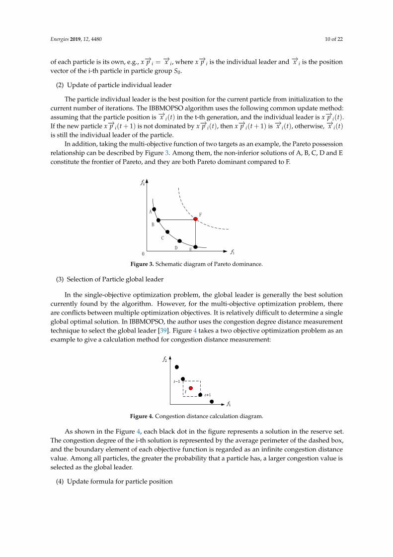
In addition, taking the multi-objective function of two targets as an example, the Pareto possessionrelationship can be described by Figure 3. Among them, the non-inferior solutions of A, B, C, D and Econstitute the frontier of Pareto, and they are both Pareto dominant compared to F.

0

A

B

C

D E

F

Figure 3. Schematic diagram of Pareto dominance.

(3) Selection of Particle global leader

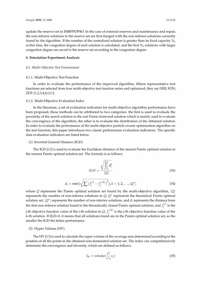
In the single-objective optimization problem, the global leader is generally the best solutioncurrently found by the algorithm. However, for the multi-objective optimization problem, thereare conflicts between multiple optimization objectives. It is relatively difficult to determine a singleglobal optimal solution. In IBBMOPSO, the author uses the congestion degree distance measurementtechnique to select the global leader [39]. Figure 4 takes a two objective optimization problem as anexample to give a calculation method for congestion distance measurement:

Figure 4. Congestion distance calculation diagram.

As shown in the Figure 4, each black dot in the figure represents a solution in the reserve set.The congestion degree of the i-th solution is represented by the average perimeter of the dashed box,and the boundary element of each objective function is regarded as an infinite congestion distancevalue. Among all particles, the greater the probability that a particle has, a larger congestion value isselected as the global leader.

(4) Update formula for particle position

Energies 2019, 12, 4480 11 of 22

The particle update formula of the traditional multi-objective particle swarm optimizationalgorithm consists of two parts: speed update and position update. In the IBBMOPSO, an improvedBBExp method [33] is proposed to update the particle position:

xi,j =

{N( rxpi,j+(1−r)xgj

2 ,∣∣xpi,j − xgj

∣∣) , U(0, 1) < 0.5

xgi,j , else(29)

In the formula, x−→p i is the individual leader of the i-th particle, and x−→g i is the global leader of the i-thparticle, where r ∈ [0, 1] in the formula.

(5) Mutation operator based on Cauchy time-varying mutation mechanism

The role of the mutation operation in the particle swarm optimization algorithm is usually toavoid the algorithm falling into the local optimum. The disturbance operator uses the mutationoperator to locate a certain dimensional decision variable of the particle to other search areas, therebyincreasing the diversity of the solution. This increases the probability that the algorithm finds theglobal optimal solution.

In the BBMOPSO, a Gaussian time-varying mutation operator is proposed based on Gaussianvariation. The specific mutation operation is shown in Algorithm 1. It can be seen that the operatorcan adjust the mutation parameter α at the same time. By adjusting the mutation probability and therange of particle activity, as the number of iterations t increases, the mutation probability and activityrange of the particle decrease gradually. Therefore, the Gaussian time-varying mutation operator hasbetter local development ability at the later stage of the algorithm iteration.

Algorithm 1 : Gaussian time varying mutation operation

1: Function Mutate(α,t,Bound,Tmax,n)2: for i=1 to N do3: if p = e(−α∗t/Tmax) > r then //r:Random number between [0,1]4: k=rand(1,n)5: range=p*(max_Bound(k)-min_Bound(k));6: xi,k = xi,k + N(0, 1) ∗ range;//N(0,1):Standard Gaussian distribution function7: end if8: end for

Due to the small variation in Gaussian variation, the ability to guide individuals to jump outof local optimal solutions is weak, so it is not productive to maintaining the diversity of solutions.In this paper, a mutation operator based on Cauchy’s time-varying mutation mechanism is proposed.The specific operation is shown in Algorithm 2. Figure 5 is a comparison of standard Gaussiansampling and Cauchy sampling probability curve. It can be seen that the range of values of thedistribution is significantly larger than the Gaussian distribution, so the use of Cauchy time-varyingvariation is beneficial to increase the diversity of the solution.

Algorithm 2 : Cauthy time varying mutation operation

1: Function Mutate(α,t,Bound,Tmax,n)2: for i=1 to N do3: if p = e(−α∗t/Tmax) > r then //r:Random number between [0,1]4: k=rand(1,n)5: range=p*(max_Bound(k)-min_Bound(k));6: xi,k = xi,k + C(0, 1) ∗ range; //C(0,1):Standard Cauthy distribution function7: end if8: end for

Energies 2019, 12, 4480 12 of 22

Figure 5. Schematic diagram of Pareto dominance.

(6) Particle out of bounds processing mechanism

When the algorithm performs the update operation and the mutation operation, the limits ofvariables are often violated. Most algorithms usually adopt the endpoint value method when dealingwith such problems, as shown below:

xk =

{min _Bound, i f xk < min _Bound(k)max _Bound, i f xk > max _Bound(k)

(30)

where min _Bound(k) and max _Bound(k) are the lower and upper bounds corresponding to the kthdimensional vector, respectively. Different from the single-objective optimization algorithm, sincenumber of objective functions in a multi-objective optimization problem is usually more than two, theoptimal solution is no longer unique, but a set of Pareto front-end solution sets. Therefore, in orderto increase the diversity of the obtained solutions, the multi-objective algorithm performs a largevariation on the solution vector, therefore the chance of limit violations will increase accordingly.The use of conventional endpoint value method for out-of-bounds processing often results in loss ofpopulation diversity, especially for optimization problems with more than three goals. In view of theabove shortcomings, this paper proposes the following particle out-of-bounds processing:

dk = β× (max _Bound(k)−min _Bound(k)) (31)

xk =

{min _Bound + rand× dk, i f xk < min _Bound(k)max _Bound− rand× dk, i f xk > max _Bound(k)

(32)

In the formula, β is the endpoint adjustment factor (the particle crossover treatment is better whentested at β = 0.01), and rand is a random number between [0, 1]. In the above-mentioned particleout-of-bounds processing mechanism, the out-of-boundary particles randomly generate a value closeto the boundary within a certain disturbance range, thus avoiding the loss of population diversitycaused by all the out-of-boundary particles taking the endpoint value, thereby increasing the diversityof the population.

(7) Update of the reserve set

At present, there are many ways to update the external reserve set. This paper uses the methodbased on the congestion distance measurement method proposed by Raquel and Sierra [40] to

Energies 2019, 12, 4480 13 of 22

update the reserve set in IMBPPOPSO. In the case of external reserves and maintenance and repair,the non-inferior solutions in the reserve set are first merged with the non-inferior solutions currentlyfound by the algorithm. If the number of the centralized solution is greater than its fixed capacity Na

at this time, the congestion degree of each solution is calculated, and the first Na solutions with largercongestion degree are saved to the reserve set according to the congestion degree.

4. Simulation Experiment Analysis

4.1. Multi-Objective Test Environment

4.1.1. Multi-Objective Test Function

In order to evaluate the performance of the improved algorithm, fifteen representative testfunctions are selected from four multi-objective test function series and optimized, they are DEB, FON,ZDT (1,2,3,4,6) [41].

4.1.2. Multi-Objective Evaluation Index

In the literature, a set of evaluation indicators for multi-objective algorithm performance havebeen proposed, these methods can be attributed to two categories: the first is used to evaluate theproximity of the search solution to the real Pareto front-end solution which is mainly used to evaluatethe convergence of the algorithm; the other is to evaluate the distribution of the obtained solution.In order to evaluate the performance of the multi-objective particle swarm optimization algorithm onthe test function, this paper introduces two classic performance evaluation indicators. The specificdata evaluation indicators are listed below.

(1) Inverted General Distance (IGD)

The IGD [42] is used to evaluate the Euclidean distance of the nearest Pareto optimal solution tothe nearest Pareto optimal solution set. The formula is as follows:

IGD =

√|Q|∑

i=1d2

i

|Q| (33)

di = min{√

∑ ( f (i)j − f ∗(k)j )2}, k = 1, 2, . . . , |Q∗| (34)

where Q represents the Pareto optimal solution set found by the multi-objective algorithm, |Q|represents the number of non-inferior solutions in Q, Q∗ represents the theoretical Pareto optimalsolution set, |Q∗| represents the number of non-inferior solutions, and di represents the distance fromthe first non-inferior solution found to the theoretically closest Pareto optimal solution, and f (i)j is the

j-th objective function value of the i-th solution in Q, f ∗(k)j is the j-th objective function value of thek-th solution. If IGD=0, it means that all solutions found are in the Pareto optimal solution set, so thesmaller the IGD the better performance.

(2) Hyper Volume (HV)

The HV [43] is used to calculate the super-volume of the coverage area determined according to theposition of all the points in the obtained non-dominated solution set. The index can comprehensivelydetermine the convergence and diversity, which are defined as follows:

IH = volume(|F|∪

i=1νi) (35)

Energies 2019, 12, 4480 14 of 22

All the values usually need to be normalized before calculating the super volume index. Whenthe calculation is completed, the obtained solution can be analyzed according to the size of the supervolume index. The larger the value of the super volume, the closer the resulting non-inferior solutionfront is to the true Pareto optimal solution, and the better the distribution of the solution. Therefore,the convergence of the Pareto solution relative to the true Pareto optimal solution frontier and thedistribution diversity of each point in the solution set can be comprehensively measured by this index.

(3) Multi-objective comparison algorithm

In this paper, a multi-objective immune algorithm, three multi-objective evolutionary algorithmsand two different multi-objective PSO algorithms are compared with the IBBMOPSO. They are NSGA2,SPEA2 , PAES2, MOPSO and BBMOPSO algorithm. The population size and the reserve size of all thealgorithms are set as the 100. Table 7 shows the other specific parameter settings for the six algorithmsincluding the IBBMOPSO algorithm.

Table 7. Parameter setting of the algorithm.

Algorithm Parameter

NSGA2

The variation coefficient of variation is set to 20The probability of variation is 3

The probability of crossover is 0.9Bidding selection

SPEA2

The exchange probability is set to 0.5The two mutation probabilities are 0.2The two crossover probabilities are 0.8

Bidding selection

PESA2The number of grids is 7

The probability of crossover is 0.5The probability of mutation is 0.5

MOPSO

The number of grids is 7The probability of mutation is 0.1

Both the individual and the global learning factors are 1 and 2The inertia weight is ω = 0.5

BBMOPSO Mutation parameter α = 10

IBBMOPSO Mutation parameter α = 10Point adjustment factor β = 0.01

4.2. Simulation Results and Performance Analysis

In order to evaluate the optimization performance of IBBMOPSO algorithm, this paper comparesit with three representative multi-objective evolutionary algorithms (NSGA2, SPEA2 [44], PESA2[45]) and two different multi-objective particle swarm optimization algorithms (MOPSO, BBMOPSO).A multi-target performance index was compared and analyzed. The algorithm performed 30 simulationexperiments on 12 test functions. In order to compare the different algorithms, a fair time measuremust be selected. The number of iterations cannot be used as a time measure, as the algorithms dodiffering amounts of work in their inner loops. It was, therefore, decided to use the number of functionevaluations (FES) as a time measure [46]. In this paper, the maximum FES (function evolutions) of atest function is set to 15,000 times.

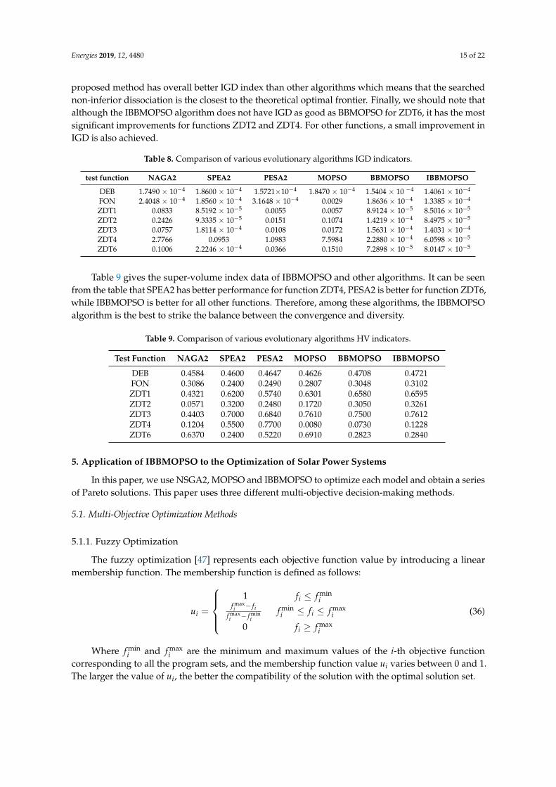
Table 8 compares the performance of IBBMOPSO algorithm and the IGD index with otheralgorithms. IGD is used to evaluate the Euclidean distance between the nearest Pareto optimal solutionand the theoretical Pareto optimal solution. The smaller the IGD value, the closer the distance of thenon-inferior solution to the optimal Pareto front end. It is obvious that IBBMOPSO has better IGDcharacteristics than other algorithms, in particular, for the functions DEB, FON, ZDT1, ZDT2, ZDT3,ZDT4, it has the best IGD characteristics, and it has the second best IGD for ZDT6. It is clear that the

Energies 2019, 12, 4480 15 of 22

proposed method has overall better IGD index than other algorithms which means that the searchednon-inferior dissociation is the closest to the theoretical optimal frontier. Finally, we should note thatalthough the IBBMOPSO algorithm does not have IGD as good as BBMOPSO for ZDT6, it has the mostsignificant improvements for functions ZDT2 and ZDT4. For other functions, a small improvement inIGD is also achieved.

Table 8. Comparison of various evolutionary algorithms IGD indicators.

test function NAGA2 SPEA2 PESA2 MOPSO BBMOPSO IBBMOPSO

DEB 1.7490 × 10−4 1.8600 × 10−4 1.5721×10−4 1.8470 × 10−4 1.5404 × 10 −4 1.4061 × 10−4

FON 2.4048 × 10−4 1.8560 × 10−4 3.1648 × 10−4 0.0029 1.8636 × 10−4 1.3385 × 10−4

ZDT1 0.0833 8.5192 × 10−5 0.0055 0.0057 8.9124 × 10−5 8.5016 × 10−5

ZDT2 0.2426 9.3335 × 10−5 0.0151 0.1074 1.4219 × 10−4 8.4975 × 10−5

ZDT3 0.0757 1.8114 × 10−4 0.0108 0.0172 1.5631 × 10−4 1.4031 × 10−4

ZDT4 2.7766 0.0953 1.0983 7.5984 2.2880 × 10−4 6.0598 × 10−5

ZDT6 0.1006 2.2246 × 10−4 0.0366 0.1510 7.2898 × 10−5 8.0147 × 10−5

Table 9 gives the super-volume index data of IBBMOPSO and other algorithms. It can be seenfrom the table that SPEA2 has better performance for function ZDT4, PESA2 is better for function ZDT6,while IBBMOPSO is better for all other functions. Therefore, among these algorithms, the IBBMOPSOalgorithm is the best to strike the balance between the convergence and diversity.

Table 9. Comparison of various evolutionary algorithms HV indicators.

Test Function NAGA2 SPEA2 PESA2 MOPSO BBMOPSO IBBMOPSO

DEB 0.4584 0.4600 0.4647 0.4626 0.4708 0.4721FON 0.3086 0.2400 0.2490 0.2807 0.3048 0.3102ZDT1 0.4321 0.6200 0.5740 0.6301 0.6580 0.6595ZDT2 0.0571 0.3200 0.2480 0.1720 0.3050 0.3261ZDT3 0.4403 0.7000 0.6840 0.7610 0.7500 0.7612ZDT4 0.1204 0.5500 0.7700 0.0080 0.0730 0.1228ZDT6 0.6370 0.2400 0.5220 0.6910 0.2823 0.2840

5. Application of IBBMOPSO to the Optimization of Solar Power Systems

In this paper, we use NSGA2, MOPSO and IBBMOPSO to optimize each model and obtain a seriesof Pareto solutions. This paper uses three different multi-objective decision-making methods.

5.1. Multi-Objective Optimization Methods

5.1.1. Fuzzy Optimization

The fuzzy optimization [47] represents each objective function value by introducing a linearmembership function. The membership function is defined as follows:

ui =

1 fi ≤ f min

if maxi − fi

f maxi − f min

if mini ≤ fi ≤ f max

i

0 fi ≥ f maxi

(36)

Where f mini and f max

i are the minimum and maximum values of the i-th objective functioncorresponding to all the program sets, and the membership function value ui varies between 0 and 1.The larger the value of ui, the better the compatibility of the solution with the optimal solution set.

Energies 2019, 12, 4480 16 of 22

For each non-dominated solution X, the normalized membership function is defined below:

uk =

N∑

i=1uk

i

M∑

k=1

N∑

i=1uk

i

(37)

where M is the number of scenarios and N is the number of objective functions. uk can be regarded asa fuzzy combination of the membership function of the non-dominated solution set. In the fuzzy set,the scheme with the highest degree of membership is defined as the best ideal solution.

5.1.2. Linear Programming Method for Multidimensional Analysis of Preference(LINMAP)

The LINMA [48] is a multi-attribute decision-making method based on the ideal solution. It isjudged by the decision maker to give a set of ordered scheme pairs that represent the scheme xk betterthan the scheme xi and the index value a∗j of the scheme xi with respect to the attribute f j, whichis established by a linear programming model to find the weight wj of each attribute and the idealsolution a∗j , then use the square of the Euclidean distance

Si =m

∑j=1

ωj(aij − a∗j ), i = 1, 2, . . . , n (38)

to rank the advantages and disadvantages of the scheme.

5.1.3. Technique for Order Preference by Similarity to an Ideal Solution(TOPSIS)

The TOPSIS method [49] is a method of sorting schemes by means of ideal solutions and negativeideal solutions of multi-objective decision problems. The so-called ideal solution is the best solution.Its various index values can reach the best value of each candidate program, while the negativeideal solution is the worst solution, and its indicators reach the worst value of the solution. Generallyspeaking, the original solution set usually does not have such ideal solution and negative ideal solution.Therefore, if there is a solution in the solution set that is very close to the ideal solution and away fromthe negative ideal solution, then the solution can be considered as the best solution in the solution set.Therefore, when the TOPSIS method is used to solve multi-objective decision problems, a measure isdefined in the objective space to measure the extent to which a solution is close to the ideal solutionand away from the negative ideal solution.

Suppose the decision problem of multi-objective systems with n scenarios and m indicators isstudied. The distance S∗i from solution Xi = (xi1, . . . , xim) to ideal solution X∗ = (x∗1 , . . . , x∗m) and thedistance S−i to X− = (x−1 , . . . , x−m) of the negative ideal solution are:

S∗i =

√√√√ m

∑j=1

(Xij − X∗j )2, i = 1, 2, . . . n; j = 1, 2, . . . , m (39)

S−i =

√√√√ m

∑j=1

(Xij − X−j )2, i = 1, 2, . . . n; j = 1, 2, . . . , m (40)

where Xi,j is the normalized value of the jth indicator of solution Xi: X∗j and X−j are the jth componentof the ideal solution X∗ and the negative ideal solution X−. The relative proximity of the merits anddemerits of the solution is C∗i :

C∗i = S∗i /(S∗i + S−i ), 0 ≤ C∗i ≤ 1, i = 1, 2, . . . , n (41)

Energies 2019, 12, 4480 17 of 22

when Xi is the ideal solution, then C∗i = 1; when Xi is the negative ideal solution, then C∗i = 0.Prioritize the schemes in order of C∗i from the largest to the smallest.

5.2. Simulation Experiments

5.2.1. Algorithm Implementation of Multi-objective Engineering Design Problem

In order to optimize, compare and analyze the two power generation system models with theselected three multi-objective algorithms, the specific implementation steps of the algorithm are givenbelow.

Step1: Set the relevant parameters of the algorithm and initialize the population.Step2: Each algorithm is optimized for each system model and get a series of Pareto solutions.Step3: For each model, the corresponding optimal solution of each objective function is selected

from the Pareto solution set obtained by the three algorithms, and then the optimal solutions obtainedby different algorithms for the same target are compared and analyzed.

Step4: Use three different multi-objective decision methods to select the ideal solution from thePareto solution set obtained by the IBBMOPSO.

5.2.2. Simulation Results for Solar Stirling Power Generation System

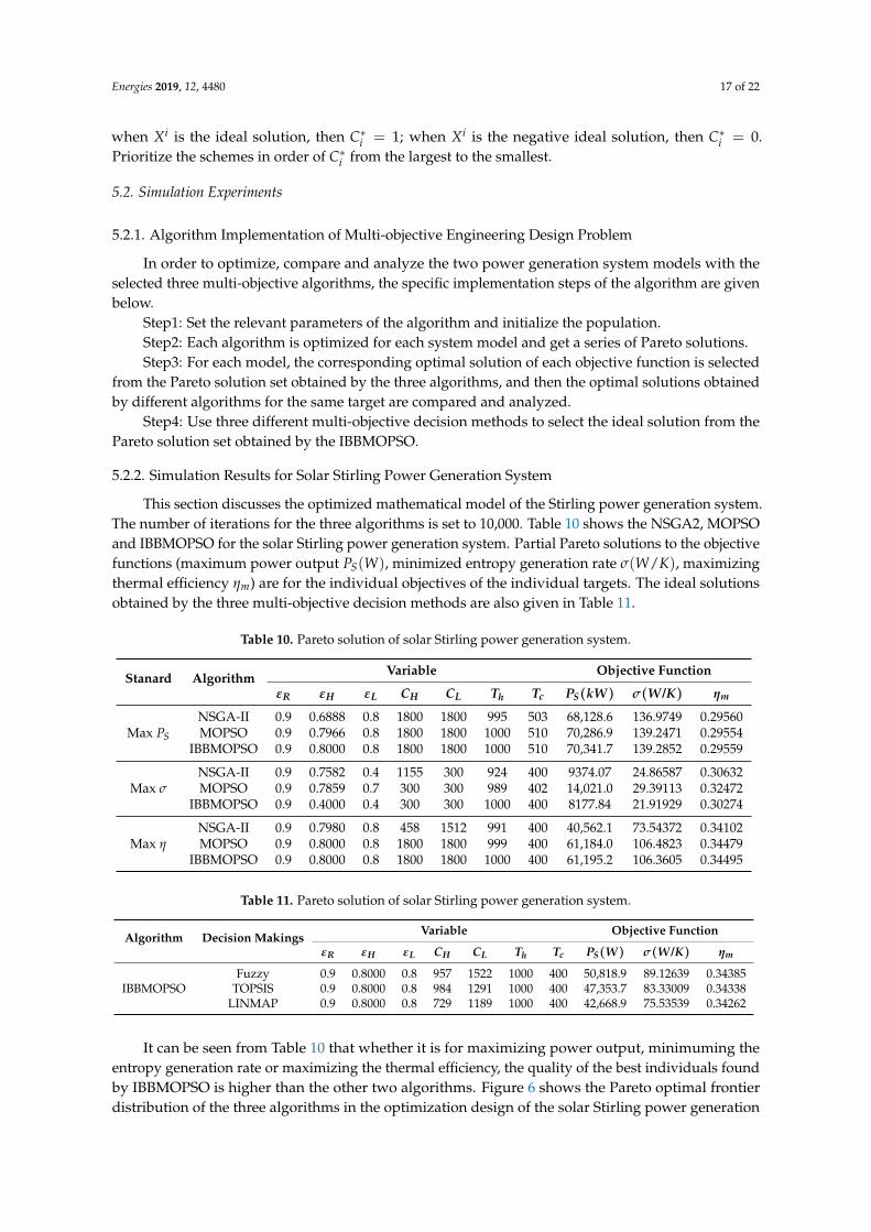
This section discusses the optimized mathematical model of the Stirling power generation system.The number of iterations for the three algorithms is set to 10,000. Table 10 shows the NSGA2, MOPSOand IBBMOPSO for the solar Stirling power generation system. Partial Pareto solutions to the objectivefunctions (maximum power output PS(W), minimized entropy generation rate σ(W/K), maximizingthermal efficiency ηm) are for the individual objectives of the individual targets. The ideal solutionsobtained by the three multi-objective decision methods are also given in Table 11.

Table 10. Pareto solution of solar Stirling power generation system.

Stanard Algorithm Variable Objective Function

εR εH εL CH CL Th Tc PS(kW) σ(W /K) ηm

Max PS

NSGA-II 0.9 0.6888 0.8 1800 1800 995 503 68,128.6 136.9749 0.29560MOPSO 0.9 0.7966 0.8 1800 1800 1000 510 70,286.9 139.2471 0.29554

IBBMOPSO 0.9 0.8000 0.8 1800 1800 1000 510 70,341.7 139.2852 0.29559

Max σNSGA-II 0.9 0.7582 0.4 1155 300 924 400 9374.07 24.86587 0.30632MOPSO 0.9 0.7859 0.7 300 300 989 402 14,021.0 29.39113 0.32472

IBBMOPSO 0.9 0.4000 0.4 300 300 1000 400 8177.84 21.91929 0.30274

Max ηNSGA-II 0.9 0.7980 0.8 458 1512 991 400 40,562.1 73.54372 0.34102MOPSO 0.9 0.8000 0.8 1800 1800 999 400 61,184.0 106.4823 0.34479

IBBMOPSO 0.9 0.8000 0.8 1800 1800 1000 400 61,195.2 106.3605 0.34495

Table 11. Pareto solution of solar Stirling power generation system.

Algorithm Decision Makings Variable Objective Function

εR εH εL CH CL Th Tc PS(W) σ(W /K) ηm

IBBMOPSOFuzzy 0.9 0.8000 0.8 957 1522 1000 400 50,818.9 89.12639 0.34385

TOPSIS 0.9 0.8000 0.8 984 1291 1000 400 47,353.7 83.33009 0.34338LINMAP 0.9 0.8000 0.8 729 1189 1000 400 42,668.9 75.53539 0.34262

It can be seen from Table 10 that whether it is for maximizing power output, minimuming theentropy generation rate or maximizing the thermal efficiency, the quality of the best individuals foundby IBBMOPSO is higher than the other two algorithms. Figure 6 shows the Pareto optimal frontierdistribution of the three algorithms in the optimization design of the solar Stirling power generation

Energies 2019, 12, 4480 18 of 22

system. In addition, the ideal and non-ideal solutions of the model and the ideal solution found bythe three multi-objective decision methods are also labelled. It can be seen from the figure that thedistribution of solutions searched by the three multi-objective algorithms is roughly the same, but thesolution searched by IBBMPSO is superior to NSGA2 and MOPSO both in scope and quality.

Figure 6. Pareto frontier map of solar Stirling power generation system.

5.2.3. Simulation Results of Solar Brayton Power Generation System

This section presents the results of the optimized mathematical model of the solar Brayton powergeneration system. The same as the solar Stirling power generation system, the maximum number ofiterations of this optimized design is set to 10000 times. Table 12 shows the single-objective optimalindividuals for the optimal power generation PB(W), optimal thermal efficiency ηm, and optimalthermal economic efficiency F for the optimal solution of the solar Brayton power generation system.It can be clearly seen from the data marked in the shaded part of the table that the solution found byIBBMOPSO and the MOPSO are the same and superior to NSGA2 in maximizing the power outputtarget. In maximizing thermal efficiency, the best solutions achieved by the IBBMOPSO is superiorto the other two algorithms. And the solution produced by the MOPSO that maximizes the thermaleconomic efficiency is optimal. The ideal solutions obtained by the three multi-objective decisionmethods are also given in Table 13.

Table 12. Pareto solution of solar Brayton power generation system.

Stanard Algorithm Variable Objective Function

εH εL εR TH TL T1 PB(kW) ηm F

NSGA-II 0.7 0.7 0.8 1000 408 596 68.4118 0.30428 0.23076MOPSO 0.7 0.7 0.8 1000 400 600 71.3588 0.30562 0.23206

IBBMOPSO 0.7 0.7 0.8 1000 400 600 71.3588 0.30562 0.23206

Max σNSGA-II 0.7 0.7 0.8 1000 408 596 68.3864 0.30433 0.23079MOPSO 0.7 0.7 0.8 1000 400 567 67.9143 0.31441 0.23776

IBBMOPSO 0.7 0.7 0.8 1000 400 566 67.8689 0.31443 0.23776

Max ηNSGA-II 0.7 0.7 0.8 1000 408 596 68.3918 0.30433 0.23079MOPSO 0.7 0.7 0.8 1000 400 564 67.3770 0.31450 0.23772

IBBMOPSO 0.7 0.7 0.8 1000 400 563 67.3226 0.31450 0.23771

Energies 2019, 12, 4480 19 of 22

Table 13. Pareto solution of solar Brayton power generation system.

Algorithm Decision Makings Variable Objective Function

εH εL εR TH TL T1 PB(W) ηm F

IBBMOPSOFuzzy 0.7 0.7 0.8 1000 400 574 69.1006 0.31360 0.23740

TOPSIS 0.7 0.7 0.8 1000 400 586 70.4810 0.31074 0.23560LINMAP 0.7 0.7 0.8 1000 400 586 70.4194 0.31095 0.23574

Figure 7 shows the Pareto frontier distribution optimized by the three multi-objective algorithmsfor the solar Brayton power generation system. It is obvious that the solution distribution of IBBMOPSOis the widest, and the solution searched by the MOPSO is relatively small. The range only coincideswith the solution decomposition searched by the algorithm in this paper, and the solution set searchedby the NSGA2 algorithm is not as good as the other two algorithms in terms of the distribution rangeand the quality of the solution.

Figure 7. Pareto frontier map of solar Brayton power generation system.

6. Conclusions and Future Work

In this paper, an IBBMOPSO algorithm has been proposed based on the BBMOPSO.The experimental results of the improved IBBMOPSO on the test functions show that the IBBMOPSOalgorithm has better convergence and distribution than other algorithms. The proposed algorithm isthen used to optimize the multi-objective mathematical model of two engineering design problems.The simulation results show that IBBMOPSO has better performance than existing popular approaches.The highlights of this paper cover the following aspects:

1. Multi-objective optimization algorithms play an increasingly important role in optimizing thepower generation systems from solar energy.

2. The IBBMOPSO is proposed based on the BBMOPSO. The experimental results showthat IBBMOPSO has better performance than other multi-objective intelligent optimizationalgorithms.

3. IBBMOPSO can provide more options for multi-objective engineering optimization problemsthan other multi-objective intelligent optimization algorithms.

The proposed IBBMOPSO algorithm has been successfully applied in the optimal design of solarStirling power generation system and solar Brayton power generation system, and it can be applied tomulti-objective engineering optimization design problems.

Energies 2019, 12, 4480 20 of 22

The MOPSO [6] still has a lot of room for improvement, for example, in developing new particleupdate strategies and new mutation strategies. The representative external storage file mechanism inthe multi-objective optimization can be further improved. Finally, the models of the two generationsystems are steady-state models under two assumptions, and the development of more accuratemodels for the optimal design also deserves future work.

Author Contributions: Q.N. received and designed the experiments; Q.N., Z.Y., H.W. and Z.S. performed theexperiments; Q.N. and H.W. analyzed the data; Q.N. and H.W. wrote the paper.

Funding: This research was funded by the National Natural Science Foundation of China (61773252) and NaturalScience Foundation of Guangdong Province (2018A030310671)

Conflicts of Interest: The authors declare no conflict of interest.

References

1. ExxonMobil. 2018 Outlook for Energy: A View to 2040. Available online: https://corporate.exxonmobil.com(accessed on 25 March 2019).

2. Li, G.Q.; Wang, H.Z.; Zhang, S.L.; Xin, J.T.; Liu, H.C. Recurrent neural networks based photovoltaic powerforecasting approach. Energies 2019, 12, 2538. [CrossRef]

3. Divina, F; Torres, M.G.; Vela, F.A.G.; Noguera, J.L.V. A comparative study of time series forecasting methodsfor short term electric energy consumption prediction in smart buildings. Energies 2019, 12, 1934. [CrossRef]

4. UN. United Nations Decade of Sustainable Energy for all 2014–2024. Available online: https://www.un.org/en/sections/observances/international-decades (accessed on 19 July 2018).

5. Vrinceanu, A.; Grigorescu, L.; Dumitrascu, M.; Mocanu, L.; Dumitrica, C.; Micu, D.; Kucsicsa, G.; Mitrica, B.Impacts of photovoltaic farms on the environment in the romanian plain. Energies 2019, 12, 2533. [CrossRef]

6. NREL. Assessment of Parabolic trough and Power Tower Solar Technology Cost and Performance Forecast; ReportNo. NREL/SR-550-34440, NREL: Golden, Co, USA, 2003; pp. 24–28.

7. Leon, L.J. Optimization of Dish Solar Collectors. Energy 1983, 7, 684–694.8. Francisco, N.; Alain, F. Thermal model of a dish Stirling systems. Sol. Energy 2009, 83, 81–89.9. Hafez, A.Z.; Ahmed, S.; Ismail, I.M. Solar parabolic dish Stirling engine system design, simulation and

thermal analysis. Energy Convers. Manag. 2016, 15, 60–75. [CrossRef]10. Caballero, G.E.C.; Mendoza, L.S.; Martinez, A.M. Optimization of a dish Stirling system working with

DIR-type receiver using multi-objective techiniques. Appl. Energy 2017, 204, 271–286. [CrossRef]11. Li, Y.; Xiong, B.Y.; Su, Y.X.; Tang, J.R.; Leng, Z.W. Particle swarm optimization-based power and temperature

control scheme for grid-connected DFIG-based dish-Stirling solar-thermal system. Energies 2019, 12, 1300.[CrossRef]

12. Anthony, P. Solar Brayton-cycle power system development. Prog. Aerosp. Sci. 1966, 16, 759–793.13. Springer, T.; Fridfdld, J. Space station freedom solar dynamic power generation. In Technology for Space

Station Evolution. Volume 4: Power Systems/Propulsion/Robotics; NASA: Washington DC, USA, 1990; Volume 4,pp. 65–81.

14. Meas, M.R.; Bello-Ochende, T. Thermodynamic design optimization of an open air recuperative twin-shaftsolar therjal Brayton cycle with combined or exclusive reheating and intercooling. Energy Convers. Manag.2017, 148, 770–784. [CrossRef]

15. Malali, P.D.; Chaturvedi, S.K.; Abdel-Salam, T. Performance optimization of a regenerative Brayton heatengine coupled with a parabolic dish solar collector. Energy Convers. Manag. 2017, 143, 85–95. [CrossRef]

16. Khan, M.S.; Abid, M.; Ali, H.M.; Amber, K.P. Comparative performance assessment of solar dish assisteds-CO2 Brayton cycle using nanofluids. Appl. Therm. Eng. 2019, 148, 295–306. [CrossRef]

17. Marler, M.T.; Arora, J.S. The weighted method for multi-objetive optimization: New insights.Struct. Multidiscip. Optim. 2010, 41, 853–862. [CrossRef]

18. Charnes, A.; Cooper, W.W. Management models and industrial applications of linear programming.Math. Comput. 1962, 16, 401. [CrossRef]

19. Ignizio, J.P.; Cavalier, T.M. Linear Programming in Single and Multiple-Objective Systems; Prentice Hall:Upper Saddle River, NJ, USA, 1982.

20. Romero, C. Handbook of critical issuues in goal programming. Eur. J. Oper. Res. 1992,62, 252.

Energies 2019, 12, 4480 21 of 22

21. Yu, P.L. A class of solutions for group decision problems. Manag. Sci. 1973 19 936–946. [CrossRef]22. Zeleny, M. Multi-Criteria Decision Making; MCGraw-Hill: New York, NY, USA, 1982.23. Konak, A.; Colt, D.W.; Smith, A.E. Multi-objective optimization using genetic algorithms: A tutorial.

Reliab. Eng. Syst. Saf. 2006, 91, 992–1007. [CrossRef]24. Mostaghim, S.; Teich, J. Strategies for finding good local guides in multi-objective particle swarm

optimization (MOPSO). In Proceedings of the 2003 IEEE Swarm Intelligence Symposium(SIS 03),Indianapolis, IN, USA, 24–26 April 2003; pp. 26–33.

25. Basu, M. Economic environmental dispatch using multi-objective differential evolution. Appl. Soft Comput.2011, 11, 2845–2853. [CrossRef]

26. Zhang, Q.F.; Li, H. MOEA/D: A Multiobjective evolutionary algorithm based on decomposition. IEEE Trans.Evol. Comput. 2007, 11, 712–731. [CrossRef]

27. Nazemzadegan, M.R.; Kasaeian, A.; Toghyani, S.; Ahmadi, M.H.; Saidur, R.; Ming, T. Multi-objetiveoptimization in a finite time thermodynamic method for dish-Stirling by branch and bound method andMOPSO algorithm. Front. Energy 2017, 8, 1701–2095.

28. Li, Y.Q.; Liao, S.M.; Liu, G. Thermo-economic multi-objective optimization for a solar-dish Brayton systemusing NSGA-II and decision making. Int. J. Electr. Power Energy Syst. 2015, 64, 167–175. [CrossRef]

29. Li, Y.Q.; Liu, G.; Liu, X.P. Thermodynamic multi-objetive optimization of a solar-dish Brayton system basedon the maximum power output, thermal efficiency and ecological performance. Renew. Energy 2016, 95,465–473. [CrossRef]

30. Kennedy, J.; Eberhart, R. Particle swarm optimization. In Proceedings of the International Conference onNeural Networks(ICNN’95), Perth, Australia, 27 November–1 December 1995; pp. 1942–1948.

31. Tripathi, P.K; Bandyopadhyay S.; Pal S.K. Adaptive multi-objective particle swarm optimization algorithm.In Proceedings of the IEEE Congress on Evolutionary Compytation, Singapore, 25–28 September 2007.

32. Praven, K.T.; Sanghamitra, B.; Sankar, K.P. Multi-Objective Particle Swarm Optimization and Multi-SwarmConcepts and Constraint Handing; Oklahoma State Unversity: Stillwater, OK, USA, 2008.

33. Zhang, Y.; Gong, D.W.; Ding, Z.H. A bare-bones multi-objetive particle swarm optimization algorithm forenvironmental/economic dispatch. Inf. Sci. 2012, 192, 213–227. [CrossRef]

34. Ahmadi, M.H.; Mohammadi, A.H.; Dehghani, S.; Barranco-Jimenez, M.A. Multi-objectivethermodynamic-based optimization of output power of Solar Dish-Stirling engine by implementing anevolutionary algorithm. Energy Convers. Manag. 2013, 75, 438–445. [CrossRef]

35. Punnathanam, V.; Kotecha, P. Multi-objective optimization of Stirling engine systems using Front-basedYin-Yang-Pair Optimization. Energy Convers. Manag. 2017, 133, 332–348. [CrossRef]

36. Li, Y.Q.; He, Y.L.; Wang, W.W. Optimization of solar-powered Stirling heat engine with finite-timethermodynamics. Renew. Energy 2011, 36, 421–427.

37. Sharma. A.; Shulka S.K.; Rai, A.K. Finite time thermodynamic analysis and optimization of solar-dishStirling heat engine with regenerative losses. J. Therm. Sci. 2011, 15, 995–1009. [CrossRef]

38. Kennedy J. Bare bones particle swarms. In Proceedings of the 2003 IEEE Swarm Intelligence Symposium,Indianapolis, IN, USA, 24–26 April 2003.

39. Deb, K.; Pratap, A.; Agarwal, S.; Meyarivan, T.A.M.T. A fast and elitist multiobjective genetic algorithm:NSGA-II. IEEE Trans. Evol. Comput. 2002, 6, 182–197. [CrossRef]

40. Raquel, C.R.; Naval, P.C. An effective use of crowding distance in multiobjective particle swarm optimization.In Proceedings of the IEEE Congress on Evolutionary Computation, Edinburgh, UK, 2–4 September 2005.

41. Zitzler, E.; Deb, K.; Thiele, L. Comparsion of multi-objective evolutionary algorithms: Empirical results.IEEE Trans. Evol. Comput. 2000, 8, 173–195.

42. Carlos, A.; Coello, C.; Margarita, R.S. A Study of the parallelization of a coevolutionary multi-objectiveevolutionary algorithm. In MICAI 2004: Advances in Artificial Intelligence; Springer: Berlin/Heidelberg,Germany, 2004.

43. Zitzler, E.; Thiele, L. Multi objective evolutionary algorithms:a comparative case study and the strengthPareto approach. IEEE Trans. Evol. Comput. 1999, 3 257–271. [CrossRef]

44. Lopez-lbanez, M.; Prasad, T.D.; Paechter, B. Multi-objective optimisation of the pump scheduling problemusing SPEA2. In Proceedings of the IEEE Congress on Evolutionary Computation, Edinburgh, UK,2–5 September 2005; pp. 435–442.

Energies 2019, 12, 4480 22 of 22

45. Saha, S.; Bandyopadhyay, S. A generalized automatic clustering algorithm in a multiobjective framework.Appl. Soft Comput. 2013, 13, 89–108. [CrossRef]

46. Van den Bergh, F.; Engelbrecht, A.P. A Cooperative Approach to Particle Swarm Optimization. IEEE Trans.Evol. Comput. 2004, 8, 225–239. [CrossRef]

47. Wang, H.O.; Tanaka, K.; Griffin, M.F. An approach to fuzzy control of nonlinear systems: Stability and designissues. IEEE Trans. Fuzzy Syst. 1996, 4, 14–23. [CrossRef]

48. Srinivasan, V.; Shocker, A.D. Linear programming techniquer for multidimensional analysis of preference.Psychometrica 1973, 38, 337–369. [CrossRef]

49. Bellman, R.; Zadeh L.A. Decision making in a fuzzy environment. Manag. Sci. 1970, 17, 141–164. [CrossRef]

c© 2019 by the authors. Licensee MDPI, Basel, Switzerland. This article is an open accessarticle distributed under the terms and conditions of the Creative Commons Attribution(CC BY) license (http://creativecommons.org/licenses/by/4.0/).