1

An Improved Block-Based Thermal Model in HotSpot 4.0 with Granularity Considerations

Wei Huang1, Karthik Sankaranarayanan1,

Robert Ribando3, Mircea Stan2 and Kevin Skadron1

Departments of 1Computer Science,2Electrical and Computer Engineering and3Mechanical and Aerospace Engineering,University of Virginia

2

Hi! I’m HotSpot Temperature is a primary design constraint

today HotSpot – an efficient, easy-to-use,

microarchitectural thermal model Validated against measurements from

Two finite-element solvers [ISCA03, WDDD07] A test chip with a regular grid of power

dissipators [DAC04] A Field-Programmable Gate Array [ICCD05]

Freely downloadable from http://lava.cs.virginia.edu/HotSpot

3

A little bit of History

Version 1.0 – a block-based model Version 2.0 – TIM added, better heat

spreader modeling Version 3.0 – grid-based model added Version 4.0 coming soon!

4

Why this work? Michaud et. al. [WDDD06] raised

certain accuracy concerns A few of those had already been

addressed pro-actively with the grid-based model

This work tries to address the remaining and does more

Improves HotSpot to Version 4.0 – downloadable soon!

5

Outline

Background Overview of HotSpot Accuracy Concerns Modifications to HotSpot Results Analysis of granularity Conclusion

6

Outline

Background Overview of HotSpot Accuracy Concerns Modifications to HotSpot Results Analysis of granularity Conclusion

7

Overview of HotSpot

Similarity between thermal and electrical physical equations HotSpot discretizes and lumps ‘electrical analogues’ (thermal R’s

for steady-state and C’s for transient) Lumping done at two levels of granularity

Functional unit-based ‘block-model’ Regular mesh-based ‘grid-model’

Thermal circuits formed based on floorplan Temperature computation by standard circuit solving

Analogy between thermal and electrical conduction

8

Structure of the `block-model’

Sample thermal circuit for a silicon die with 3 blocks, TIM, heat spreader and heat sink (heat sources at the silicon layer are not shown for clarity)

9

Outline

Background Overview of HotSpot Accuracy Concerns Modifications to HotSpot Results Analysis of granularity Conclusion

10

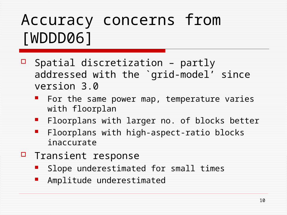
Accuracy concerns from [WDDD06] Spatial discretization – partly addressed

with the `grid-model’ since version 3.0 For the same power map, temperature varies

with floorplan Floorplans with larger no. of blocks better Floorplans with high-aspect-ratio blocks

inaccurate Transient response

Slope underestimated for small times Amplitude underestimated

11

Other issues and limitations

Forced isotherm at the surface of the heat sink

Temperature dependence of material properties – not part of this work

12

Outline

Background Overview of HotSpot Accuracy Concerns Modifications to HotSpot Results Analysis of granularity Conclusion

13

Block sub-division

Version 3.1 – a block is represented by a single node

Version 4.0 – sub-blocks with aspect ratio close to 1

14

Heat sink boundary condition

Version 3.1 – single convection resistance, isothermal surface

Version 4.0 – parallel convection resistances, center modeled at the

same level of detail as silicon

15

Other modifications Spreading R and C approximation formulas

replaced with simple expressions (R = 1/k x t/A, C = 1/k x t x A)

Distributed vs. lumped capacitance scaling factor – 0.5

‘grid-model’ enhancements – apart from the above: First-order solver upgraded to fourth-order

Runge-Kutta Performance optimization of the steady-state

solver

16

Outline

Background Overview of HotSpot Accuracy Concerns Modifications to HotSpot Results Analysis of granularity Conclusion

17

Experiment 1 – EV6-like floorplan

18

Results with good TIM (kTIM = 7.5W/(m-K))

5

10

15

20

25

30

Icac

he

Dcach

e

Bpred

DTB

FPAdd

FPReg

FPMul

FPMap

IntM

apIn

tQ

IntR

eg

IntE

xec

FPQ

LdStQ ITB

Re

lativ

e T

em

pe

ratu

re (

K)

ANSYS

HS4.0

HS3.1

FF3d

-5

-4

-3

-2

-1

0

1

2

Icac

he

Dcach

e

Bpred

DTB

FPAdd

FPReg

FPMul

FPMap

IntM

apIn

tQ

IntR

eg

IntE

xec

FPQ

LdStQ ITB

Te

mp

era

ture

Err

or

to A

NS

YS

(K

)

HS4.0 error

HS3.1 error

FF3d error

19

Results with worse TIM (kTIM = 1.33W/(m-K))

20

25

30

35

40

45

50

55

60

65

Icac

he

Dcach

e

Bpred

DTB

FPAdd

FPReg

FPMul

FPMap

IntM

apIn

tQ

IntR

eg

IntE

xec

FPQ

LdStQ ITB

Re

lati

ve

Te

mp

era

ture

(K

)

ANSYS

HS4.0

HS3.1

FF3d

-4

-2

0

2

4

6

8

10

12

14

Icac

he

Dcach

e

Bpred

DTB

FPAdd

FPReg

FPMul

FPMap

IntM

apIn

tQ

IntR

eg

IntE

xec

FPQ

LdStQ ITB

Te

mp

era

ture

Err

or

to A

NS

YS

(K

)

HS4.0 error

HS3.1 error

FF3d error

20

Transient response – bpred

0

2

4

6

8

10

12

14

1.00E-05 1.00E-04 1.00E-03 1.00E-02 1.00E-01

time (s)

rela

tive

tem

per

atu

re (

K)

ANSYS

HS4.0

HS3.1

Heat Flux(W/mm^2)

Transient response for different power pulse widths applied to the branch predictor. Power density is 2W/mm2 (kTIM = 7.5W/(m-K)). Other blocks have zero power dissipation.

21

Experiment 2 – 1 mm2 square heat source

Version 3.1 Version 4.0

22

Results

0

20

40

60

80

100

120

140

0 0.005 0.01 0.015 0.02square heat source size (m)

rela

tiv

e t

em

pe

ratu

re (

K)

ANSYS

FF3d

HS3.1

HS3.1 AR

HS4.0

Center temperature for different heat source sizes with a power density of 1.66W/mm2 – (a) with good TIM (kTIM = 7.5W/(m-K)) (b) with

worse TIM (kTIM = 1.33W/(m-K))

0

50

100

150

200

250

0 0.005 0.01 0.015 0.02

square heat source size (m)

rela

tiv

e t

em

pe

ratu

re (

K)

ANSYS

FF3d

HS3.1

HS3.1 AR

HS4.0

23

Transient response: high power density, worse TIM

0

20

40

60

80

100

120

140

160

180

0.00001 0.0001 0.001 0.01 0.1

time (s)

Re

lati

ve

Te

mp

era

ture

(K

)ANSYS

HS4.0

HS3.1

FF3d

Transient temperature response for 1mm x 1mm source with 10Watts with worse TIM material (kTIM = 1.33W/(m-K)).

24

Outline

Background Overview of HotSpot Accuracy Concerns Modifications to HotSpot Results Analysis of granularity Conclusion

25

Spatial filtering

The Norton equivalent first-order thermal spatial RC circuit

Low-pass filter in the spatial domain Blocks with high power density need not be hot

spots (when small enough)

26

Spatial filtering – continued...

Thermal RC is distributed First-order approximation not sufficient 3-ladder RC (similar to HotSpot) approximates well

Comparison of 3-ladder thermal spatial RC model and ANSYS simulation for different heat source sizes.

27

Outline

Background Overview of HotSpot Accuracy Concerns Modifications to HotSpot Results Analysis of granularity Conclusion

28

Summary, limitations and caveats This work acknowledges and addresses the

concerns in [WDDD06] `grid-model’ [DAC04] had addressed part of

the discretization aspect earlier HotSpot 4.0 addresses remaining and does

more Careful use of vertical layers necessary,

material properties’ dependence on T not modeled

Soon to be available at http://lava.cs.virginia.edu/HotSpot

29

Questions?

30

Backup – ATMI [MoBS07] Analytical model, has good accuracy A diversity in modeling is good for the

community Vis-a-vis HotSpot – advantages

Immune to spatial discretization Disadvantages

Less flexibility (esp. in vertical layers) Computationally intensive (esp. when looking for

temperature with a particular property)

31

Backup – Transient response: high power density, good TIM

0

20

40

60

80

100

120

0.00001 0.0001 0.001 0.01 0.1

time (s)

Rel

ativ

e T

emp

erat

ue

(K)

ANSYS

HS4.0

HS3.1

FF3d

Transient temperature response for 1mm x 1mm source with 10Watts power and a good TIM (kTIM = 7.5W/(m-K)).

32

Backup – Transient response: low power density, good TIM

0

0.5

1

1.5

2

2.5

3

3.5

4

4.5

5

0.0001 0.001 0.01 0.1

Time (s)

Re

lati

ve

Te

mp

era

ture

(K

)

ANSYS

HS3.2

HS3.1

FF3d

Transient temperature response for a 7mm x 7mm source with 10Watts power and a good TIM (kTIM = 7.5W/(m-K)).

33

Backup – Granularity (1)

A first-order electrical RC circuit

34

Backup – Granularity (2)

The Thevenin equivalent first-order thermal spatial “RC” circuit.