1 An improved model and a heuristic for capacitated lot sizing and scheduling in job shop problems O. Poursabzi 1 , M. Mohammadi* , 1 , B. Naderi 1 1 Department of Industrial Engineering, Faculty of Engineering, Kharazmi University, Tehran, Iran Email addresses: [email protected](O. Poursabzi), [email protected](M. Mohammadi), [email protected](B. Naderi) Abstract This paper studies the problem of capacitated lot-sizing and scheduling in job shops with a carryover set- up and a general product structure. After analyzing the literature, the shortcomings are easily realized; for example, the available mathematical model is unfortunately not only non-linear but also incorrect. No lower bound and heuristic is developed for the problem. Therefore, we first develop a linear model for the problem on-hand. Then, we adapt an available lower bound in the literature to the problem studied here. Since the problem is NP-hard, a heuristics based on production shifting concept is also proposed. Numerical experiments are used to evaluate the proposed model and algorithm. The proposed heuristic is assessed by comparing it against other algorithms in the literature. The computational results demonstrate that our algorithm has an outstanding performance in solving the problem. Keywords: lot-sizing and scheduling; job shop; Sequence-Dependent; Lower bound; Heuristic. 1. Introduction Production management is a multi-disciplinary task simultaneously involving many factors. Lot-sizing and scheduling are the two main parts of production planning and control system. Lot-sizing deals with determining the production amount of each product at each production run, often over a finite multi- period horizon. A lot indicates the quantity of a given product processed on a machine continuously without interruption after its correspondent set-up. On the other hand, scheduling is to determine the production sequence in which the products are manufactured on a single machine [1]. The integrated problem provides a more effective production plan compared to the cases in which two problems are solved hierarchically by inducing the solution of the lot-sizing problem in the scheduling level. Simultaneous lot-sizing and scheduling is essential especially when sequence-dependent set-up costs and times occur [2]. In many of the production environments, switching between production lots of two different products triggers operations such as machine adjustments, tool changing and cleansing procedures. These set-up operations are usually dependent on the sequence [2]. In order to avoid
Transcript
1
An improved model and a heuristic for capacitated
lot sizing and scheduling in job shop problems
O. Poursabzi1, M. Mohammadi*, 1, B. Naderi1
1Department of Industrial Engineering, Faculty of Engineering, Kharazmi University, Tehran, Iran
A feasible solution for this example is shown in Figure 2. The numbers on the arcs signify the quantity
of the lower level products.
Please Insert Figure 2
The indices, parameters and variables of the multi-level general lot sizing and scheduling problem
(MLGLSP)_MM are shown below:
Indices:
i, j, k, l, n Product or item type.
f Indicates micro-periods of per machine in each macro-period.
Indicates a specific micro-period of per machine in each macro-period in accordance with
the micro-period segmentation of the machine.
Machine type.
T Macro-period.
Parameters:
T Planning horizon.
N Number of different products.
M Number of different machines (or different stages) available for production.
Production coefficient, which indicates how many units of product j are required to produce
a unit of product i.
BM A large number.
Capacity of machine m required for the production of a unit of product j (in time units per
quantity unit)
Capacity of machine m required as input in order to produce one unit of the shadow product
j (in time units per quantity unit); also referred to as the input coefficient.
Available capacity of each machine m in macro-period t (in time units)
External demand for product j at the end of macro-period t (in units of quantity).
Storage costs unit rate for product j in macro-period t.
6
Cost unit rate for maintaining the setup condition of machine m for product j (in money
units per time unit).
Production costs for producing one unit of product j on machine m in the macro-period t (in
money units per quantity unit).
Sequence dependent setup costs for the setup of machine m from the production of product
i to the production of product j (in money units); for i j , , 0ij ms applies and for
, , 0ij mi j s .
Sequence dependent setup times for the setup of machine m from the production of product
i to the production of product j (in time units); for i j , , 0ij mw applies and for
,, 0ij mi j w .
Variables:
Stock of product j at the start of the planning horizon (in quantity units).
Stock of product j at the end of the planning horizon (in quantity units).
Production quantity of product j in the micro-period f of macro-period t on machine m (in
quantity units).
Quantity of shadow product j in the micro-period f of macro-period t on machine m (in
quantity units).
Binary variable which indicates whether micro-period f of macro-period t is an idle period
for machine m in which the setup condition for product j is maintained ( ) or
not ( ); with
product j has the function of a shadow function.
Decision Variables:
Binary variable which indicates whether to set up machine m from the production of product i
to the production of product j in micro-period f of macro-period t on machine m
( ) or not ( ).
Binary variable which indicates whether machine m is set up ( ) or not (
) in micro-period f of macro-period t for the production of product j.
The MILP formulation of the problem is as follows (Equation 1-20).
7
Objective function:
∑∑ ∑ ∑∑
∑∑ ∑ ∑ ∑∑
(1)
Subject to:
∑ ∑
∑ ∑ ∑
(2)
8
[ ] [ ( )
* ∑ ∑
∑
+]
[ ] * ( )
∑ ∑( ∑
)+
(3)
∑∑
∑∑∑
∑∑
(4)
(5)
(6)
9
∑
(7)
∑
(8)
∑
(
∑
)
(9)
(10)
∑
(11)
( )
(12)
( )
(13)
(∑∑
)
(14)
10
∑∑
(15)
(16)
{ } (17)
{ } (18)
{ } (19)
(20)
In this model, Equation 1 represents the objective function which minimizes the sum of the sequence-
dependent set-up costs, the storage costs, the production costs and the costs of maintaining the machine’s
set-up conditions in the planning horizon. Constraint 2 ensures the balance of demand supply in each
period. Two types of product's demand are taken into account in this model: 1) the external demand for
products that must be provided at the end of each macro-period, 2) the internal demand of the products
required for the production of high-level products in the product structure which must be satisfied within
the macro-period. The external demand ( ) and the internal demand (∑ ∑ ∑
) of a
macro-period for the product j must be provided by previous macro-period’s stock and the production
quantity of product j in current macro-period. Here, the first period is exception, since the demands have
to be provided by production.
Constraint 3 is used so as to consider vertical interaction in the proposed model. In this equation, each
typical product is produced before its direct substitute product in one macro-period. The left side of
constraint 3 is equal to the time between the beginning of the macro-period t and the end of the
production of product j if micro-period f is a production micro-period for product j; otherwise, it is zero.
In other words, if the value is not positive, the left side of constraint 3 becomes zero. The right side of
constraint 3 is equal to the time between the beginning of period t and the beginning of the production of
product i if micro-period f is a production micro-period for product i, else it is a big number. In other
words, if the value is positive, the right side of constraint 3 is zero.
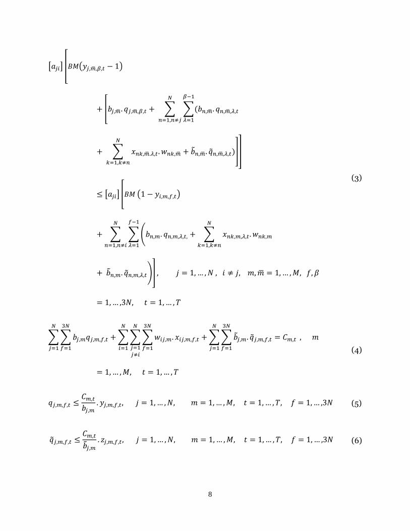
Constraint 4 shows the capacity constraints of machines during a macro-period. Constraint 5 indicates
the relation between set-up and production processes and obtains an upper bound (UB) for production
quantity. Constraint 6 determines the duration of idle times. It also yields a UB for the duration of the idle
times. Constraints 7 and 8 guarantee that in each macro-period, at most a single lot is produced for each
product. To achieve this aim, Fandel & Stammen-Hegene [2] applied ∑ ∑
11
but these constraints cannot satisfy this aim. Assume a problem with N=2, M=3, T=2,
, Product_rout{1}={1, 3}, Product_rout{2}={1, 2, 3}. Also suppose that all products must be
produced in period 1, then:
Due to the above expanding equation, for each product in each period only one stage of product rout
can be run on, so the products demand cannot be satisfied. However, by applying equations 7 and 8 in the
proposed model, the mentioned deficiency is rectified.
Equation 7
Equation 8
Constraints 9-11 bound the micro-periods in each macro-period to one of the following three
positions; i.e., production, set-up and idle micro-period. To ensure this purpose, Fandel & Stammen-Hegene [2] presented the following equation in their
paper:
∑ ∑ (
)
In case with m=1, , t=1, M=3 the generated constraint could be written as follows:
In contrast, the generated form of equation 9 can be written like so:
12
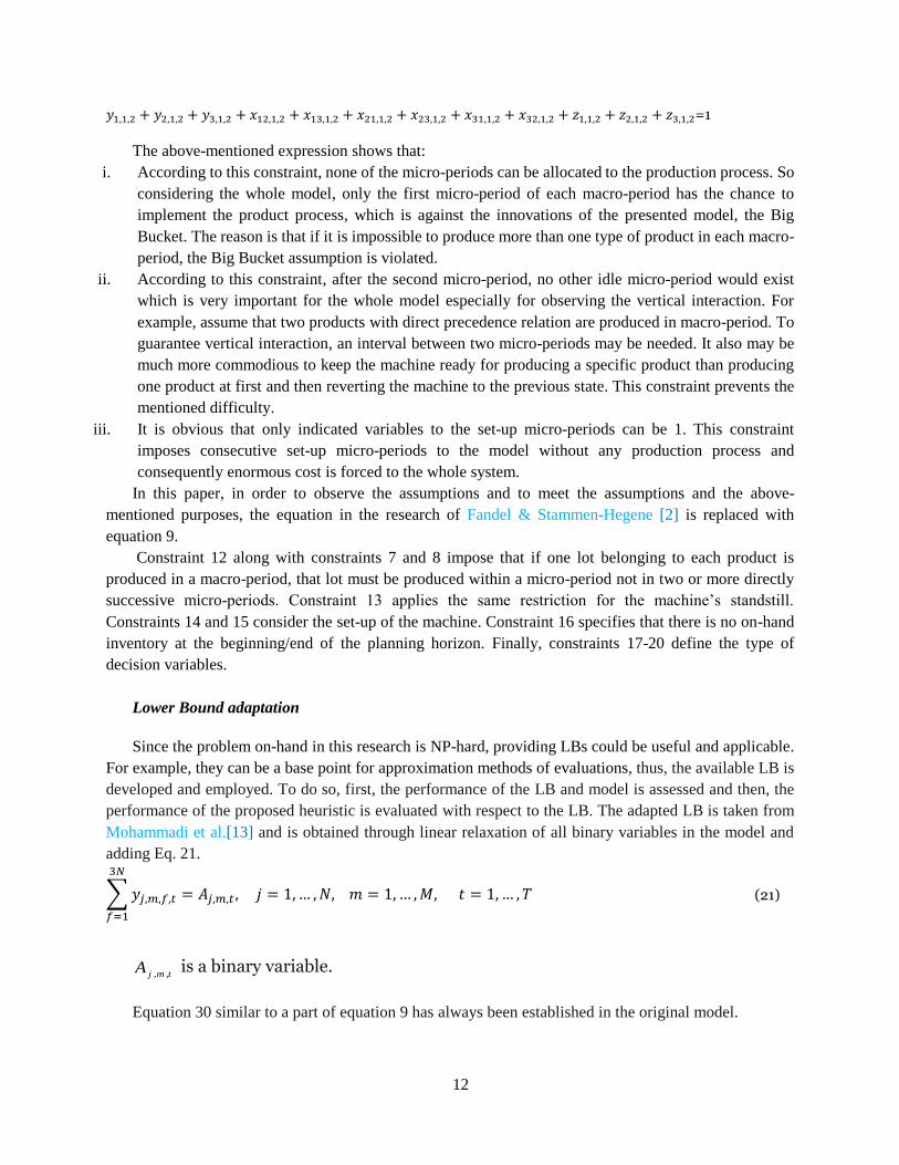
=1
The above-mentioned expression shows that:
i. According to this constraint, none of the micro-periods can be allocated to the production process. So
considering the whole model, only the first micro-period of each macro-period has the chance to
implement the product process, which is against the innovations of the presented model, the Big
Bucket. The reason is that if it is impossible to produce more than one type of product in each macro-
period, the Big Bucket assumption is violated.
ii. According to this constraint, after the second micro-period, no other idle micro-period would exist
which is very important for the whole model especially for observing the vertical interaction. For
example, assume that two products with direct precedence relation are produced in macro-period. To
guarantee vertical interaction, an interval between two micro-periods may be needed. It also may be
much more commodious to keep the machine ready for producing a specific product than producing
one product at first and then reverting the machine to the previous state. This constraint prevents the
mentioned difficulty.
iii. It is obvious that only indicated variables to the set-up micro-periods can be 1. This constraint
imposes consecutive set-up micro-periods to the model without any production process and
consequently enormous cost is forced to the whole system.
In this paper, in order to observe the assumptions and to meet the assumptions and the above-
mentioned purposes, the equation in the research of Fandel & Stammen-Hegene [2] is replaced with
equation 9.
Constraint 12 along with constraints 7 and 8 impose that if one lot belonging to each product is
produced in a macro-period, that lot must be produced within a micro-period not in two or more directly
successive micro-periods. Constraint 13 applies the same restriction for the machine’s standstill.
Constraints 14 and 15 consider the set-up of the machine. Constraint 16 specifies that there is no on-hand
inventory at the beginning/end of the planning horizon. Finally, constraints 17-20 define the type of
decision variables.
Lower Bound adaptation
Since the problem on-hand in this research is NP-hard, providing LBs could be useful and applicable.
For example, they can be a base point for approximation methods of evaluations, thus, the available LB is
developed and employed. To do so, first, the performance of the LB and model is assessed and then, the
performance of the proposed heuristic is evaluated with respect to the LB. The adapted LB is taken from
Mohammadi et al.[13] and is obtained through linear relaxation of all binary variables in the model and
adding Eq. 21.
∑
(21)
, ,j m tA is a binary variable.
Equation 30 similar to a part of equation 9 has always been established in the original model.
13
After relaxing the binary variables, neither equation 3 nor 14 has no significant influence on the
model, since the left side of equation 3 would be a big negative number and the right side of equation 3 or
14 would be a big positive number owing to the values of the relaxed variables . It means that by
relaxing the binary variables, equation 3 or 14 is always satisfied without imposing any obligation so as to
guarantee vertical interaction in the model. Thus, in calculating of the LB, equation 3 or 14 can be
eliminated from the model.
3. The proposed Shifting-Based heuristic
Since the problem on hand is NP-hard, it cannot be solved in a reasonable computational time using
the exact classical methods. To rectify such a difficulty, employing heuristics is the best alternative [30].
The proposed heuristic in this research is based on part (or entire) of product lot shifting from a specific
period to others and includes 4 phases: initializing, smoothing, improving and merging mechanisms.
In initializing mechanism, an initial solution is generated through ignoring the capacity constraints. If
this initial solution is infeasible, the smoothing mechanism is used to obtain a feasible solution based on
the concept of product shifting. The improving mechanism starts from the obtained feasible solution of the
smoothing mechanism and try to improve this solution. In merging mechanism phase, the produced lots
obtained from improving procedure are integrated with the goal of reducing the set-up cost. If, the
solution obtained from the merging mechanism phase is infeasible, it will be used as the initial solution of
the next iteration.
The algorithm repeats until the stopping criterion is met. The general outline of the proposed heuristic
is shown in Figure 3. The 4 mechanisms are described as follows.
Please Insert Figure 3
3.1. Initialization
In this mechanism, one initial solution is generated. It should be noted that three decisions should be
made in the problem under consideration: products to be produced at each period, the lot-size of each
product and product sequence on each machine. Obviously, these decisions are determined in any
solution. The used heuristic search in this research defines the first two decisions and tries to improve
them while the product sequence of a given solution is defined using a dispatching rule. Figure 4 shows
how a solution is encoded in the proposed heuristic in terms of a numerical example.
Please Insert Figure 4
{
First, the initial solution is generated for the incapacitated version of the problem. This solution is then
becomes feasible using the soothing mechanism, if it violates the capacity constraint. To this end,
Wagner-Whitin algorithm is used for each product. The algorithm is first applied to items with
independent demand dj,t. It is then applied to each item 2,...,j N with both independent and
dependent demands.
Those products should be produced during the studied period according to the encoding scheme must
have the following conditions. Let P(j) be a set including all products that can be produced i.e., there is
14
sufficient amount of its prerequisites. The sequence can be determined considering the following rules
among those products which have necessary conditions for production. In each step, the products in
which the examined machine is one of the production process steps, are selected. At the beginning steps
of production, if a given product has any prerequisite then a required amount of necessary materials
should be available in order to make sure that the product is considered as a candidate for the operation.
Also, if the examined machine is in any step except the first step then the operation on the product should
be completed in previous steps. Due to [2], those products in lower levels of general product structure
(GPS), have a greater number of demands and also there are many products which are dependent on these
mentioned products for initiating their production process; therefore, they are assigned higher priority for
production.
If there is more than one output from the previous level, the High priority product is the one with
lower average set-up cost. The average set-up cost for product j on machine m is derived from ∑
∑ ∑ . If the examined product is the first produced product of the considered machine during the
current macro-period, its set-up could be performed in previous period(s) by concerning cost and source.
In this case, the carryover option for set-up should be applied to the next period.
A well-known property, called zero-switch property [31], for the incapacitated lot-sizing problem can
be defined as follows: there is an optimal solution for the incapacitated lot-sizing problem (the problem
GCLSP without resource constraints) where one can write
Product quantity(j,t)*Inventory(j,t-1)=0
or
(∑ ∑
) (∑ ∑
)
Using this property, the production quantity of each item in its production periods can be calculated as
such.
Step 1: For any item j and period t, if Ej,t=0 then set Product quantity(j,t)=0
Step 2: For any item j any periods t1<t2≤T, if Ej,t1=Ej,t2 =1 and Ej,t=0 for all t1<t<t2 then
∑ ( ∑
)
(22)
In other words, if a product is produced in a given period, the demand of that period as well as all
periods up to the next production period of that item should be satisfied. Since no backlogging is
assumed, all items are produced in the first period, i.e.:
.
In CLSP, the optimal solution may do not include zero-switch property, since it also depends on the
available capacity of machines. Hence, the solution, derived from this property, is used as a base solution
to generate a feasible solution considering capacity constraints. This procedure is carried out using a
heuristic explained in the next subsection.
3.2. Smoothing mechanism
The initial solution (P1) may be infeasible owing to violating capacity constraint. In this case, the
smoothing mechanism aims to generate a feasible solution named P2 through shifting products from an
infeasible period to other periods. Note that a period is infeasible if the capacity constraint is violated.
15
In an infeasible period t, a portion of product quantity named qit out of total production quantity of
item j in period t is transferred to another period tl. For each item j produced in an infeasible period t, two
quantities are considered to shift to period tl:
Wj,tl: The maximum production quantity of product j in period t; which guarantees that inventory
constraints are still satisfied. This amount depends on whether tl > t or tl < t.
Qj,t: The quantity of production j in infeasible period t: it eliminates the resource overload (machine
capacity) m in period t by shifting this quantity to another;
,(∑
∑ ∑
∑
)
⁄ - (23)
In Eq (23), the comparison is made only for positive values. Note that the amount Qi,t indicates that
overuse of resource k in the period t could be reduced to zero if there is a quantity less than Wi,tl,. The
smoothing mechanism includes the following two steps.
3.2.1. Backward shifts
In this mechanism, the production shifting from each period to earlier periods is analyzed. The
procedure starts from the last period and continuous toward the first period. If the period is infeasible, a
portion of selected produced product is moved to earlier periods so that period t becomes feasible. It
should be pointed out that the production shifting process is checked to all earlier periods and the best one
is selected. The product is also selected by the ratio test which will be discussed later. If no feasible
solution is found by shifting the first selected product, the procedure applies to the next product. For an
infeasible period t, a quantity Qj,t out of the entire production amount of product j in period t is shifted to
earlier target period tl where τ ≤ tl ≤ t-1. Note that we have
τ = max{1, the last period among periods prior to period t in which component j is produced}.
The production shifting increases the product stock in a period. In order to meet the inventory balance
constraints, the portion of the shifting must be held:
,
{
⁄ } - (24)
It is noteworthy to indicate that there always exists a component r whose entire production can be
moved to an earlier period, { | }, since
, where P(r) is the set of all immediate predecessors of component r. In other words,
the entire product of an item can be moved from the current period to earlier periods when none of its
components is produced in the current period.
The selection of quantity, component and target period (qj,t, j ,tl) is based on the ratio test derived from
cost variation calculation and resource usage. If the procedure continues to the first period and no feasible
solution is found, the forward shifting is applied. Otherwise, procedure P2 terminates.
16
3.2.2. Forward shifts
This mechanism deals with the production shifting from a given period to later periods. It starts from
the first period to the last and intends to shift a portion of a product to subsequent periods so as to make it
feasible. Similar to the backward shift, the production shift to all earlier periods is checked and the best
one is selected. The products are selected one by one and the procedure applies to the next product if no
feasible solution is found.
For an infeasible period t, a quantity qj,t out of the entire production amount of product j in period t is
shifted to later target period tl, where t+1 ≤ tl ≤ τ and τ = min{T, the first period among periods
subsequent to period t in which component j is produced}.
Similar to backward shifts, the selection of quantity, moved component and target period are also
based on the ratio test. The production shift to the next periods reduces the inventory from period t to tl-1;
therefore, the inventory balance should be guaranteed. Eq. (25) is used to determine the shifted quantity to
the next periods.
{ } (25)
After these shifting, if a feasible solution is found, P2 terminates, otherwise, the backward shift
procedure should be applied again.
3.2.3. Ratio test
This procedure aims at selecting the shifted quantity, component and target period (qj,t, j, tl ), i.e., the
quantity qj,t out of the entire production amount of component j in period t should be moved to an earlier
or later target period tl. The values of (qj,t, j, tl) are chosen so that the following ratio (Eq. (26)) is
minimized.
(26)
The Extra Cost (Eq. (27)) is calculated as follows:
(27)
By shifting qj,t from period t to tl , the cost variation calculated by Additional Cost (Eq. (28)) is
imposed.
*( ) (∑( ∑
)
)+ (28)
The first term of the right hand side of Eq. (28) calculates the production cost variation. The second
and third terms compute the inventory cost variation and set-up cost variation, respectively. Total Cost is
the current system costs which is derived from the model objective function. The Additional cost
parameters can be expressed as follows.
{
}
17
{
}
{
}
{
}
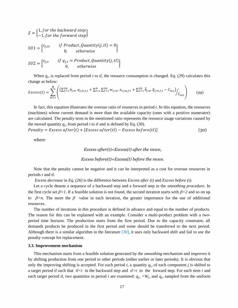
When qj,t is replaced from period t to tl, the resource consumption is changed. Eq. (29) calculates this
change as below:
∑ ((∑
∑ ∑
∑
)
⁄ )
(29)
In fact, this equation illustrates the overuse ratio of resources in period t. In this equation, the resources
(machines) whose current demand is more than the available capacity (ones with a positive numerator)
are calculated. The penalty term in the mentioned ratio represents the resource usage variations caused by
the moved quantity qj,t from period t to tl and is defined by Eq. (30).
[ ] (30)
where
Excess after(t)=Excess(t) after the move,
Excess before(t)=Excess(t) before the move.
Note that the penalty cannot be negative and it can be interpreted as a cost for overuse resources in
periods t and tl.
Excess decrease in Eq. (26) is the difference between Excess after (t) and Excess before (t).
Let a cycle denote a sequence of a backward step and a forward step in the smoothing procedure. In
the first cycle set =1. If a feasible solution is not found, the second iteration starts with =2 and so on up
to =n. The more the value in each iteration, the greater importance for the use of additional
resources.
The number of iterations in this procedure is defined in advance and equal to the number of products.
The reason for this can be explained with an example. Consider a multi-product problem with a two-
period time horizon. The production starts from the first period. Due to the capacity constraint, all
demands products be produced in the first period and some should be transferred to the next period.
Although there is a similar algorithm in the literature [30], it uses only backward shift and fail to use the
penalty concept for replacement.
3.3. Improvement mechanism
This mechanism starts from a feasible solution generated by the smoothing mechanism and improves it
by shifting production from one period to other periods (either earlier or later periods). It is obvious that
only the improving shifting is accepted. For each period t, a quantity qj,t of each component j is shifted to
a target period tl such that tl<t in the backward step and tl>t in the forward step. For each item i and
each target period tl, two quantities in period t are examined: qj,t =Wj,t and qj,t sampled from the uniform
18
distribution U[0, wi,tl]. One reason for selection of the second random value is that different solutions may
be obtained with the same initial point. Moreover, the costs vary over time and shifting a quantity qjt <
wi,tl may result in a lower cost. Any candidate set (q,i,tl) in period t among all candidates which minimizes
the Extra cost is chosen. The procedure terminates when no feasible and improving solution is found.
3.4. Merging procedure
The purpose of this procedure is to further diversify the search. In this procedure, the entire production
of an item j in a given period is moved to another period tl (either earlier or later) in which that item is
produced. The aim of production lots merging is to reduce the set-up and production cost. The item
production process can be shifted to period tl if this item’s lot in the current period is equal to Wj,tl which
is calculated by Eq. (24) for tl<t, and by Eq.(25) for tl>t. If the obtained solution is feasible, the
improvement procedure (P3) is applied to enhance the solution’s quality. Otherwise, the obtained solution
is used as a new starting point for the Smoothing procedure (P2).
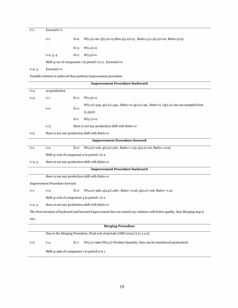
In the rest of this section, an example is illustrated so as to clarify the proposed heuristic steps.
Assume a problem with N=4, M=1, T=4 and except parameters a and D, the other of the parameters'
value are similar to Section 3.
[
]
Smoothing Procedure-backward
t=4 Excess(t)=0
t=3 Excess(t)>0
i=1, 2, 3 tl=2 W(i,2)=0, the production shift of these components from current period to period is
impossible
i=4 tl=2 W(4,2)=890 and Q(4,2)=1480 (Since Q>W, Q is not Considered q(4,2)=890, ratio=0.74
tl=1 W(4,1)=890 then q(4,1)=890, ratio=1.15
Shift q=890 of component 4 in period 3 to 2, so Excess(t)>0 then continue
i=1 tl=2 W(1,2)=0
i=2 tl=2 W(2,2)=120, Q(2,2)=100 then q(2,2)=100 , Ratio=1.91; q(2,2)=120, Ratio=1.97
tl=1 W(2,1)=0
i=3 tl=2 W(3,2)=120, Q(3,2)=100 then q(2,2)=100 , Ratio=1.91; q(2,2)=120, Ratio=1.97
tl=1 W(3,1)=0
Shift q=100 of component 2 in period 3 to 2, Excess(t)=0
t=2 Excess(t)=0
Smoothing Procedure-forward
19
t=1 Excess(t)>0
i=1 tl=2 W(1,2)=20, Q(1,2)=15 then q(1,2)=15 , Ratio=3.2; q(1,2)=20, Ratio=3.03
tl=3 W(1,2)=0
i=2, 3, 4 tl=2 W(i,2)=0
Shift q=20 of component 1 in period 1 to 2, Excess(t)=0
t=2, 3 Excess(t)=0
Feasible solution is achieved thus perform Improvement procedure
Improvement Procedure-backward
t=4 no production
t=3 i=1 tl=2 W(1,2)=0
i=2 tl=2 W(2,2)=445, q(2,2)=445 , Ratio>0; q(2,2)=99 , Ratio>0 (q(2,2)=99 was sampled from
[1,350])
tl=1 W(2,1)=0
i=3 there is not any production shift with Ratio<0
t=2 there is not any production shift with Ratio<0