93
AN INSIGHT INTO THE THEORETICAL BACKGROUND OF: SOIL STRUCTURE INTERACTION ANALYSIS OF DEEP FOUNDATIONS Dr. Eng. Özgür BEZGİN İSTANBUL January 2010
| Date post: | 03-May-2018 |
| Category: |
Documents |
| Upload: | nguyendieu |
| View: | 214 times |
| Download: | 1 times |

AN INSIGHT INTO THE THEORETICAL
BACKGROUND OF:
SOIL STRUCTURE INTERACTION ANALYSIS
OF DEEP FOUNDATIONS
Dr. Eng. Özgür BEZGİN
İSTANBUL
January 2010

ii
TABLE OF CONTENTS
LITERATURE REVIEW AND THEORETICAL BACKGROUND ............................................ 1
1.1 Introduction .......................................................................................................................... 1
1.2 Sub-grade Models ............................................................................................................... 1
1.3 Winkler’s Hypothesis ......................................................................................................... 3
1.4 Fundamentals of Soil-Structure Interaction (SSI) Modeling .................................. 4
1.4.1 Flexural Behavior of the Sub-structure ................................................................ 6
1.4.1.1 Simple Beam Theory ............................................................................... 6
1.4.1.2 Timoshenko Beam Theory ....................................................................... 7
1.4.1.3 Beam Under Transverse and Axial Loads ................................................ 9
1.4.1.4 Soil Supported Beam Under Transverse and Axial Loads ...................... 11
1.4.2 Modeling Subgrade Reaction ................................................................................ 13
1.4.2.1 Two Dimensional Subgrade Models .................................................... 13
1.5 Deep Foundations ............................................................................................................. 24
1.6 Analysis and Design of Deep Foundations Under Lateral Loads ....................... 27
1.6.1 Subgrade Reaction Approach .................................................................................... 28
1.6.1.1 Elastic Soil Behavior ............................................................................. 28
1.6.1.2 Plastic Soil Behavior ............................................................................. 31
1.6.2 Elastic Continuum Approach ...................................................................................... 33
1.7 Load Displacement Characteristics of Soil .............................................................. 36
1.7.1 Variation of Soil Elastic Modulus with Depth .................................................... 38
1.7.1.1 Field Tests ........................................................................................... 41
1.7.1.2 API Procedure for Developing P-Y Curves ............................................. 45

iii
1.8 SSI Modeling of Deep Foundations.............................................................................. 51
1.8.1 Finite Element Modeling in SSI ................................................................................... 51
1.8.2 Finite Element Analysis Overview ............................................................................. 54
1.8.3 Types of Elements .......................................................................................................... 60
1.8.3.1 Beam Elements .......................................................................................... 60
1.8.3.2 Spring Elements ........................................................................................ 61
1.8.3.3 Solid Elements ........................................................................................... 62
1.8.3.4 Infinite Elements ........................................................................................ 64
1.8.4 Inherent Problems Associated with Finite Elements ........................................... 65
1.9 Time Integration Procedures ........................................................................................ 68
1.10 Soil Modeling .................................................................................................................. 71
1.10.1 Mohr-Coulomb Yield Criterion ................................................................................. 73
1.10.2 Drucker-Prager Yield Criterion ............................................................................... 75
1.10.2.1 Extended Tresca Criterion ....................................................................... 75
1.10.2.2 Extended von Mises Criterion .................................................................. 76
1.10.3 Friction and Dilatation in Soils and Lade Criterion ............................................ 78
1.11 Contact Modeling .......................................................................................................... 81
REFERENCES ................................................................................................................................ 86

1
LITERATURE REVIEW AND THEORETICAL BACKGROUND
1.1 Introduction
Civil engineering structures always have some structural element in contact with the
ground. The structural element that is in contact with the ground could sometimes be
the structure itself or could be a structural component such as concrete footings, mat
foundations, piles, and drilled shafts. Every structure is built to resist a combination
of loads. This resistance must be developed within serviceability and strength limits.
The forces that the structure is designed to withstand must be transferred to a wider
domain in order to achieve static equilibrium. In other words, the structure itself must
be supported. This wider domain is the ground and the load transferring structural
elements are the foundations.
When forces are applied externally to the structure, internal forces develop and both
components must deform and move in a compatible manner. This is because neither
the displacements of the structure nor the ground displacements are independent of
each other as a result of their physical contact. Because of this mutual dependence of
the structure and soil behavior, these types of problems are broadly referred to as
soil-structure interaction (SSI) problems.
1.2 Sub-grade Models
Sub-grade models are mathematical models to investigate the SSI problems and to
approximate the behavior of soil under externally applied loads. A subgrade model is
generally the simplest mathematical model that will produce acceptably accurate
estimates of the key parameters for a particular SSI application.
SSI is present to some degree in every problem where a structural element is in
contact with the ground. However, the current state of practice in geotechnical and

2
structural engineering includes many instances where SSI is neglected and the
structural element and ground are analyzed independently of each other. This is done
for analytical simplicity since SSI analyses are statically indeterminate i.e. in addition
to satisfying force and moment equilibrium, compatibility of displacements must also
be considered explicitly to solve an SSI problem. The incentive to simplify the
analyses and not consider SSI for routine applications is very strong in practice.
Development of a sub-grade model is a process that has certain stages or steps,
which can be summarized as follows:
1. Qualitative investigation of the problem in order to understand how the
structure behaves and which parameters are needed in order to define these
behaviors.
2. Identification and ranking in order of importance the parameters of interest that
needs to be included in a sub-grade model for that application.
3. Obtaining the parameters through experimental testing.
4. Discretization of the sub-grade and solving the established mathematical
relationships using some type of numerical method.
The proposed numerical method in this study is the finite-element method (FEM),
which is a method to solve an algebraic equation.
A sub-grade model involves a qualitative description of the analyzed subject,
identifying the necessary parameters that are related to the qualitative analyzes,
providing the numeric values for these parameters through previously conducted
experiments and representing the structure by elements that embody the included
parameters. All these steps are just approximations of reality, so the overall SSI
model is an approximation. The question is what the level of this approximation should

3
be, and given the level and strength of the existing analytic tools, can the existing
models be improved with little or no extra effort.
Although the development of a model involves correct execution of all these steps,
the single most important step would be to provide the correct numeric values for the
parameters used in the model because any model is as good as the data provided. A
simple model with accurate input is preferred to an elegant model with poor input
data.
SSI analysis using mathematical models is dated back as early as the 19th century
with the publication of a mathematical expression known as Winkler’s Hypothesis.
1.3 Winkler’s Hypothesis
Winkler's Hypothesis is still used by the civil engineers as the primary subgrade
model in SSI applications. It is an approximation of the soil reaction to a distributed
loading, such that it takes into account the major contributor to the soil resistance i.e.
the soil stiffness. The hypothesis has originated from slabs resting on soil and has
then been modified for other applications such as deep foundations. The hypothesis
suggests that the soil develops a resistance to loading as discrete and independent
elements, thus disregarding the shearing that exists between the soil layers. Figure
1.1 represents the Winkler’s approximation.
The soil resistance per unit area is related to soil displacements through a constant
called the coefficient of sub-grade reaction. The spring model is an application that
makes use of Winkler’s Hypothesis to represent the soil with spring elements for a
given structure where the spring constant depends on the coefficient of sub-grade
reaction, and geometric and stiffness properties of the structure. The coefficient of

4
sub-grade reaction is also an important parameter around which various SSI models
are developed.
Figure 1.1- Winkler’s approximation of soil resistance for a slab on grade.
Inter-soil layer shear coupling i.e. the transfer of shear between soil layers parallel to
the direction of the loading, which is disregarded by the Winkler’s Hypothesis is not
only present in soil, but also the fundamental determinant how the load bearing and
load transfer occur within the soil. Therefore any mathematical model that does not
include this shearing has an inherent disadvantage.
The developed theories and models have stemmed from consideration of slabs
resting on soil. However the logic and theory behind the findings from the research
and analysis of slabs resting on soils can be modified and applied to foundations of
various types, of which the deep foundations will be of interest in this book.
1.4 Fundamentals of Soil-Structure Interaction (SSI) Modeling
The load-displacement behavior of a structural component (foundation,subgrade and
superstructure) is physically linked to, and thus dependent on the behavior of the

5
other two. Ideally, the foundation-subgrade-superstructure system should always be
analyzed as a single problem.
The force-displacement characteristics of a SSI problem can be summarized as
follows:
The force applied by the superstructure on the substructure q(x,y,z,t) which
can be defined in terms of location and time depending on whether the force is
static or dynamic in nature. (In 2-D static loading: q(x,y) )
The reaction of the soil to the loading imposed on it by the superstructure
p(x,y,z,t). (In 2-D static loading p(x,y) )
The settlement within the supporting soil in order to generate the necessary
reaction w(x,y,z,t).
The main difference in the philosophy of various subgrade models is whether these
three components are considered as independent and separate entities or mutually
related and dependent entities.
In the traditional approach to solve the SSI problem, the subgrade reaction, p(x,y,z,t),
is considered as an external force whose magnitude must be assumed or postulated
mathematically in some manner at the beginning of the analysis. Also, in the
traditional approach, the subgrade reaction is considered as independent and
discrete reactions. Because p(x,y) has such a crucial role as an input parameter in
the simplified analyses used in practice, it turns out to be very useful to define a new
subgrade stiffness parameter, k(x,y), that is called the coefficient of subgrade
reaction and is defined as:
(1)

6
The flexural (bending) behavior of the foundation element has a great influence on the
structural modeling of SSI applications. The flexural behavior of the substructure as
well as the soil stiffness properties determines the distribution of the soil reaction and
the displacements and settlements within the structure as a whole.
1.4.1 Flexural Behavior of the Sub-structure 1.4.1.1 Simple Beam Theory
The basic form of the matrix formulation for beam flexure is:
(2)
Where the coefficients are:
[S] = Stiffness matrix
{d} = Displacement vector
{q} = Load (force) vector.
Figure 1.2 illustrates the basic components of a beam subjected to applied loads q(x).
Figure 1.2 – Beam under distributed loading.
In developing the traditional solution (Euler or simple beam theory) for the
displacement of this beam in the z direction due to the transverse load q(x), three
assumptions and approximations are made:

7
1. The initial (undeformed) geometry of the beam is used (linear analysis).
2. A vertical plane through the beam cross-section will remain plane (Plane
sections remain plane).
3. Vertical downward displacements (deflections) of the beam w(x) are relatively
small.
The resulting differential equation defining the behavior of a beam constrained by the
above three assumptions is:
(3)
Which assuming EI(x) = constant, becomes: Using the stiffness-matrix concept stated in Equation 2, the flexural stiffness matrix,
(4)
[S], for a simple beam is:
(5)
Where l = beam length. 1.4.1.2 Timoshenko Beam Theory
One of the assumptions introduced during the formulation of simple beam theory is
the "plane-sections remain-plane" assumption. In reality, internal shear stresses
develop within a beam during bending. These stresses cause sections that are

8
perpendicular to the longitudinal axis of the beam and initially planar, to warp as the
beam displaces downward under load. This warp can be visualized as horizontal
displacements relative to a plane through the beam's longitudinal axis. The result of
this warping is that beam displacements are always somewhat greater than those
based on the traditional planar assumption. The additional component of
displacement, i.e. the magnitude of displacement over and above that estimated
based on simple beam theory, is referred to as shear deformations while the primary
component of displacement is called bending deformations (Timoshenko and Gere
1972). An analysis of a beam that takes account of the beam deformations due to
bending and shear is sometimes referred to as a Timoshenko beam.
On the other hand, an Euler (simple) beam takes into consideration the beam
deformations due to bending only. The theoretical influence of shear deformations
can be understood using the flexural stiffness matrix, [S]. First, a new dimensionless
parameter, αv that incorporates the shear effects is defined as follows:
(6)
Where:
Av = Shear area of the beam,
G = Elastic shear modulus of the beam
The remaining terms were defined previously.
The flexural stiffness matrix, [S], incorporating shear effects can then be expressed
as:

9
(7)
Comparing a Timoshenko beam to traditional simple beam, it is clear that the effect of
shear stresses is to reduce the magnitude of most of the coefficients in the stiffness
matrix thus making the beam less stiff in flexure which increases beam deflection
under a given load. Shear effects are always present in every beam and thus simple
beam theory always underestimates beam deflections. However, theory and
experience indicate that simple beam theory produces quite acceptable results for
the majority of practical applications involving slender bending elements. Shear
effects become important primarily as the beam span-to-depth ratio decreases
although the composition and cross-sectional geometry of the beam influence results
as well (Roark and Young 1975).
1.4.1.3 Beam Under Transverse and Axial Loads
Under simple beam theory, the axial force has no effect on the flexural behavior of the
beam and only causes axial stress within, and axial strain of the beam. In fact, for a
simple beam the load P can be increased without theoretical limit (linear-elastic
material behavior is assumed) and will never cause buckling of the beam.

10
Figure 1.3 – Beam under transverse and axial loading.
A beam (or column) under combined transverse, q(x), and axial compressive, P, loads
will develop additional displacements, forces and moments not predicted by simple
beam theory and eventually causes the beam to buckle. This behavior is referred to
as the P-∆ effect because the axial force P causes the additional displacements.
A basic analysis performed using traditional simple-beam theory is referred to as a
first-order analysis. An analysis performed considering the P-∆ effect is referred to
as a second-order analysis. First-order analysis is based on the initial, un-deformed
geometry of a structure and second-order analysis takes into account the deformed
geometry.
(8)
It can be seen that the flexural effects of the axial force, P, on the deformed shape of
the beam are reflected in the second term on the left-hand side of Equation. Also, if P
= 0 the beam-column equation reverts back to the simple-beam equations. If the shear
is neglected for simplicity, the flexural stiffness matrix, [S], for a true beam-column is:

11
(9)
The effect of the axial force, P, on the flexural behavior of the beam is to modify the
flexural stiffness of the beam. A compressive force reduces all terms in the matrix and
makes the beam more flexible. On the other hand, a tension force increases all terms
in matrix and thus stiffens a beam. The beam-column equation has been used
extensively in geotechnical applications such as laterally loaded deep foundations.
1.4.1.4 Soil Supported Beam Under Transverse and Axial Loads
For structural elements bearing on a subgrade, it is necessary to extend the beam-
column equations to include the forces involved with soil deformations. Figure 1.4
shows the general case of either a simple beam or beam-column supported on a
subgrade. The beam-subgrade contact stress (subgrade reaction) is denoted by p(x).
Note that the variation of p(x) along the structural element is not necessarily zero and
in most cases it will be continuous.
Figure 1.4 –Soil supported beam under transverse and axial loads.

12
The differential equations for a simple beam and beam-column for this problem are,
respectively:
(10)
(11)
Alternatively, using the stiffness matrix formulation, both the simple beam and beam-
column can be expressed using the same equation as only the stiffness matrix itself is
different:
(12) Where {p} is called the subgrade reaction vector. At this point all that remains is to describe the p(x); which is the soil reaction to
external loadings, in a parametrically compatible way with the remainder of the
components of the modified beam-column equation. The attraction of Winkler's
Hypothesis is that all the effects of {p} can be expressed in terms of the
displacements, {d}, alone. This means that {p} is eliminated as a variable and
Equation 12 can be used to define the behavior of a simple beam or beam-column on a
Winkler subgrade. This simplicity is the reason why the Winkler’e Hypothesis has
found such an extensive use in geotechnical engineering. Various ways in which the
subgrade reaction, p(x,y) or {p}, can be modeled either by direct assumption or using
a subgrade model, are studied by considering what variables can be considered and
solved explicitly and whether a first order or a second order analysis is required.

13
1.4.2 Modeling Subgrade Reaction The beam equations that reflect the various aspects of the beam stiffness
components developed in the previous section constitutes only a single aspect of the
SSI. In order to have a complete sub-grade model, the next step is to define the soil
stiffness component.
The development of the majority of subgrade modeling concepts is based on a couple
of key factors. One is that the geotechnical capacity of most SSI applications is
governed by the serviceability limit state, SLS, of the subgrade as opposed to its
ultimate limit state, ULS. The other is that in most SSI applications the subgrade
affecting the behavior of the structural element is a 3-D continuum that can, with good
approximation, be taken to be a quasi-solid even though it is not a true solid. With tthe
availability of commercial finite element modeling programs the analysis of a highly
indeterminate numerical model is possible. However, significant effort has been given
in modeling the physical nature of SSI in 2-D.
These models break the interaction problem into its components and take them into
account individually. Therefore, prior to the introduction of the FEM aspects of SSI, a
summary of the 2-D models will be given.
1.4.2.1 Two Dimensional Subgrade Models
2-D subgrade models involve some mathematical expression that is stated only at the
interface between the structural element and subgrade. The primary challenge of 2-D
models is to incorporate the subgrade stratigraphy, material properties and their
variations that occur with depth (z axis) into the various terms of the mathematical
expression.

14
Surface-element models (SEM) involve use of simple and approximate mathematical
functions to define the subgrade behavior. Winkler's Hypothesis is a very simple
example of SEM. There have been improvements in order to reflect the different
physical aspects of the SSI with mechanical elements such as springs, flexural
elements (beams in one-dimension (1-D), plates in 2-D), shear only layers, dashpots,
friction devices and membranes. Such subgrade models will be referred to as
mechanical models. The evolution of mechanical models started with the simplest and
then become more complex with time.
Starting in 1950s an alternative approach to developing SEMs evolved in which the
starting point was the three sets of partial-differential equations (compatibility,
constitutive, equilibrium) governing the behavior of the indeterminate and linear-
elastic continuum. Simplifying assumptions were then applied to these equations to
yield a SEM, which are simplified-continuum models.
1.4.2.1.1 Mechanical Models
1.4.2.1.1.1 Single-Parameter Models (Winkler's Hypothesis)
Winkler's Hypothesis assumes that the settlement, w, at an arbitrary point i the
subgrade surface is caused only by the applied vertical normal stress (subgrade
reaction) at that point, p. Furthermore, p and w are linearly related. Mathematically,
this is expressed as:
(13)
Where kw is defined as Winkler's coefficient of subgrade reaction at point i. Winkler's
Hypothesis is what is called a single-parameter subgrade model because only one

15
Parameter; kw, is necessary to define its behavior. For an arbitrary number of points
over the subgrade surface, the general form of Winkler's Hypothesis is:
(14)
However, this equation does not reflect the true nature of the problem and is only
partially valid because the settlement of any given point on an actual subgrade
surface is influenced by the applied pressure p(x,y) at all points on the subgrade
surface. For a Winkler subgrade, only the applied pressure at that point as defined in
Equation (14) causes the settlement at a given point. One drawback is that the soil is
not treated as a continuum, but rather as a series of discrete resistances, second
these isolated resistances are assumed to be constant and third the effect of the
strength characteristics of the foundation element on the subgrade reaction is
overlooked. From demonstrations on actual foundation elements (Horvath 1988,
1993; Liao 1995; Vesic and Johnson 1963) as well as the very simple idealized limiting
cases of a perfectly flexible or perfectly rigid foundation element (Horvath 1979,
1983a), the displacement and the pressure variation beneath the elements are found
to be variable depending on the stiffness of both the soil and the foundation elements.
However, taking into consideration the time that these approximations had to be
made i.e. the absence of advanced computational tools; Hetenyi (1946) presented a
solution based on the Winkler’s Hypothesis. The development of this solution is as
follows:
Figure 1.5 shows a straight beam supported along its entire length by an elastic
medium and subjected to vertical forces. If a term k is defined in terms of coefficient
of subgrade reaction and the width of the beam then:

16
(15)
By considering the equilibrium of the element in Figure 1.5 and summing the forces in
the vertical direction, Hetenyi (1946) presents for p=kwo.w(x) :
(16)
Figure 1.5 –Prismatic beam supported by an elastic medium.
Making use of the relationship Q = dM /dx and using the differential equation of a
beam in bending:
(17)
Alternatively using the stiffness matrix formulation, the behavior of the beam can be
expressed as:
(18)
Where the flexural stiffness matrix, [S], of the beam is for a simple (Euler) beam or for
a Timoshenko beam as desired. For a certain value of Winkler's coefficient of
subgrade reaction, the equation can be presented as:
(19)
This can be simplified as:
(20)
pdx=k.wdx
qkwdx
dQor0q.dxk.wdxdQ)(QQ
Mdx
wdEIandqk.w
dx
Md
dx
dQ2
2
2
2

17
Where [S'] is the modified flexural stiffness matrix that is defined as follows:
(21)
The fundamental shortcoming in Winkler's Hypothesis as expressed in its basic
definition is that it cannot replicate the mechanism of "load spreading" that develops
within an actual subgrade due to the development of shear stresses. Visualized using
the spring analogy for Winkler's Hypothesis, the "springs" of an actual subgrade are
not independent as Winkler's Hypothesis assumes, but are coupled or linked together
so that an applied load at some point i produces settlement not just at point i but
adjacent ones (i-1, i+1, etc.) as well. Conversely, the settlement at some point i is the
result of applied loads not just at point i but at other points as well (which may or may
not be adjacent). Thus it is convenient to state that the absence of "spring coupling"
in Winkler's Hypothesis is its single most significant shortcoming as a subgrade
model. Therefore, any improvement to Winkler's Hypothesis must incorporate spring
coupling in some manner.
1.4.2.1.1.2 Multiple-Parameter Models
Multiple-parameter models can be visualized as containing two or more physical
components compared to the single component (layer of springs) used to model
Winkler's Hypothesis. These physical components are related to the displacement
w(x,y) in a direction perpendicular to the subgrade surface and parallel with the
direction of the applied load p(x,y). The basic element is one where the resistance to
an applied load, p(x,y), is proportional to w(x,y) which symbolizes the spring stiffness
characteristics of the soil.

18
(22)
where cpi and cwi are constant coefficients that vary depending on the model and may
be zero in some cases. These coefficients are composed of the various properties of
the mechanical elements used in that model, i.e. spring stiffness, k; shear layer
stiffness, g; membrane tension, T; and plate flexural stiffness, D. The next term is the
shear coupling that was previously overlooked and which exists within the soil under
loading. The highest-order physical element defined in developing mechanical models
is used to define the mathematical behavior of an Euler flexural element. This would
be a plate in 2-D or a simple beam in 1-D. The plate or beam is assumed to be linear-
elastic in its behavior.
Table 1.1 summarizes the composition of mechanical models in order of their
increasing mathematical complexity and, therefore, presumed accuracy as a
subgrade model.
Table 2.1 – Mechanical subgrade models and characteristics.
Subgrade model Physical elements used to visualize model
Winkler's Hypothesis springs
Filonenko-Borodich deformed, pretensioned membrane + springs
Pasternak's Hypothesis shear layer + springs
Loof's Hypothesis springs + shear layer + springs
Modified Pasternak
Haber-Schaim plate + springs
Hetényi springs + plate + springs
Rhines springs + plate + shear layer + springs
Winkler's Hypothesis is a single-parameter model. The mathematically identical
Filonenko-Borodich model and Pasternak/Loof Hypothesis are the lowest level
multiple parameter models.
Equation (22) is the general form for all the listed models with various coefficients
reflecting the physical components of the model.
)yw(x,cy)w(x,cy)w(x,cy)p(x,cy)p(x,cy)(x, 4
w
2
ww
4
p
2
p 3212ip

19
The Pasternak/Loof Hypothesis is the simplest mechanical model that inherently
incorporates subgrade shear (spring coupling). The 1-D version of Equation (22) for a
Pasternak/Loof subgrade is:
(23)
Where g is the shear stiffness of the shear layer and k is the spring stiffness of the
spring layer. Combining Equation (23) with that of a beam on a subgrade yields
equation (24), which is the equation of a true beam-column supported on a Winkler
subgrade where the shear coupling is considered.
(24)
Examination of equations (23) and (24) indicates that all the spring-coupling effects
inherent in a Pasternak/Look subgrade are replaced by a fictitious tensile force of
magnitude g per unit width of the beam. This force is applied to the longitudinal axis of
the beam parallel to the horizontal x-axis (Figure 1.3). Thus g acts opposite of the
sense of P, which is shown in Figure 1.4. From the perspective of the flexural stiffness
matrix of a beam, a tensile force makes the beam appear to be stiffer than it actually
is. Thus it can be seen qualitatively that the consideration of shear effects (spring
coupling) in a subgrade, compared to a Winkler subgrade without such effects has
the result of reducing differential settlements of the foundation element.
1.4.2.1.2 Simplified-Continuum Models
The evolution of single parameter models into multi parameter models, and the
analytical procedures associated with them, have initiated the development of
“simplified continuum models” in which the development of the models always starts
with the most complex case (the complete set of partial-differential equations defining

20
the behavior of a linear-elastic continuum) after which various assumptions are made
with regard to these equations in order to render the remaining equations easy to
solve in an exact, closed-form manner. Such assumptions typically involve certain
stresses and strains to be zero.
Development of simplified-continuum models to date has taken two main paths:
1. Reissner (1958, 1967) pioneered an application of this concept to produce what
is referred to as the Reissner Simplified Continuum (RSC) model. The concept
first proposed by Reissner was extended by Horvath (1979) to produce two
simpler models that are called the Pasternak-Type Simplified Continuum
(PTSC) and Winkler-Type Simplified Continuum (WTSC) models.
2. Vlasov and Leont'ev (1960) presented a less-direct application of the simplified
elastic continuum concept. This alternative approach involves using variational
calculus. The complication of this approach is that in addition to making
simplifying assumptions about an elastic continuum as Reissner did, an
arbitrary function must be assumed to define how vertical displacements vary
as a function of depth.
The highest order simplified-continuum model that has been developed to date is the
Reissner Simplified Continuum. Reissner solved the problem of an isotropic,
homogeneous elastic continuum of infinite lateral extent but finite thickness that is
shown in figure 1.6. This layer was underlain by a rigid base and subjected to a
surface pressure p. In developing the necessary equilibrium conditions within this
semi-bounded media, Reissner assumes that certain stresses ( x , y xy) within the
elastic layer resulting from the applied pressure to be zero. The resulting partial
differential equation relating the surface pressure p and surface displacement W is:

21
(25)
C1, C2 and C3 are related to E, G and H.
Figure 1.6 – Reissner’s simplified elastic continuum.
The governing equation of the RSC for an isotropic, homogeneous linear-elastic
continuum of finite thickness H is:
(26)
E and G are the elastic constants (Young's and shear modulus respectively) for the
continuum (Horvath 1979).
Reissner Simplified Continuum and Modified Pasternak (Kerr) models are
theoretically equivalent as approximations for an elastic continuum. Figure 1.7 shows
these two models as applied to deep foundations.
pCpWCWC 2
3
2
21
y
x
z H

22
Figure 1.7 – (a)-Modified Pasternak model for deep foundations. (b)-Reissner type simplified elastic continuum for deep foundations
Modified Pasternak model consists of an incompressible shear layer of stiffness g
sandwiched between two spring layers, the governing equation for this model is
(Horvath 1988d, 1989c):
(27)
Where ku and kl are the spring stiffnesses of the upper and lower spring layers
respectively. Equating the constant coefficients in equations (26) and (27) results in
three equations for three unknowns (g, ku and kl), the results of which are:
(28)
(a)
Inter-spring shear layer component
Spring component
M
V
(b)
V
M
T
Artificial boundary for displacements

23
Since the two spring layers act in series, the equivalent overall spring stiffness, keq, is:
(29)
The overall equivalent "spring" stiffness in the three simplified-continuum models
(Reissner, Pasternak-Type and Winkler-Type) is E ÷ H.
With this result it is seen that the Winkler’s coefficient, or the coefficient of sub-grade
reaction is the elastic modulus divided by the thickness of a layer of isotropic,
homogeneous linear-elastic material where all stresses and strains within that
material other than normal stresses and strains in the vertical direction are assumed
to be zero. Coefficient of subgrade reaction can also be viewed as the rate of change
of elastic modulus with depth.

24
1.5 Deep Foundations
Deep foundations are subjected to compression loads mainly due to dead and live
loads from the superstructure, and uplift and lateral loads due primarily to wind and
earthquake. Piles and drilled shafts are the two main examples for deep foundations.
When the type of soil that is within the limits of reach of conventional slab-on-grade
foundations is insufficient to provide proper support to the superstructure, longer
and separate structural systems called deep-foundations must be used to transfer the
loads from the superstructure to the soil with the sufficient strength.
Drilled shafts are cast-in-place concrete piles with or without steel reinforcement or
encasement. They are also referred to as large diameter bored piles. The structural
element is not driven but formed in a pre-augered hole. In cases where the hard soil
or rock is beyond the reach of driven piles, and when large number of piles are
needed to achieve the necessary resistance to lateral loads, or the soil is difficult to
penetrate via driving piles without the risk of damaging the pile itself, drilled shafts
are used to achieve a load path between the superstructure and the firm strata.
One major difference between piles and drilled shafts is that in piles the structural
loads can be introduced into soil gradually via friction and the pile tip does not
necessarily have to lie on top of a firm stratum. However for drilled shafts, the tip
almost always lies on top of firm strata, and even sometimes buried into it (belled
shape shafts or socketed shafts. Figure 1.8 shows different drilled shafts and
associated load transfer mechanisms.

25
Figure 1.8 –Type of drilled shaft and underream shapes (Woodward et.al “Drilled Pier Foundations” 1972).
Deep foundations have to traverse a significant depth of soil to reach their point of
termination. Not only the properties of soil that is relevant to SSI such as E, G, , and
varies with depth, but the absence or presence of groundwater becomes a factor that
needs to be considered in strength calculations. The theory developed for SSI using
slab-on-grade foundations is still valid, however those conclusions should be
upgraded with the relevant changes specific to deep-foundations.

26
Typically for shallow foundations, the dominant load components are axial loads and
shear, which are transmitted to the soil through the footing, thereby creating the
bearing stresses on the soil. These axial loads and shear are due to gravity loads and
lateral loads. Deep foundations on the other hand frequently experience a third type
of behavior from the superstructure other than axial load and shear that develops
“bending” resistance of the deep foundations. Lateral loads and moments acting on
the shafts in addition to the axial loads cause this bending resistance. Due to the
slenderness of the drilled shaft, flexural behavior in lateral load analysis becomes
important. The load bearing capacity of the soil has to be validated both in terms of
axial resistance and lateral resistance and the design of a deep foundation has to
satisfy both the vertical loading and the lateral loading requirements. However, the
soil that influences the axial resistance and the lateral resistance of the shaft is
located at different depths along the shaft. The firm rock-soil layer at the toe of the
shaft influences the axial capacity of the SSI system, on the contrary, the top soil
layers that extend to approximately 5 to 6 times the shaft diameter below the ground
surface control the lateral response of the shaft. Most shaft deflections occur at the
ground surface, but these layers have the least resistance to lateral loadings.
Structural failure of a drilled shaft under lateral loads is usually in the form of
excessive lateral displacements, which eventually affects the super-structure. If the
shaft cannot receive the necessary support from the upper soil layers, it will deflect
until the necessary support to lateral loading is created through bending stresses
within the shaft. In order to remain within deflection serviceability limits and prevent
excessive deflections, the lateral resistance of the SSI must be concentrated within
the top layers of the soil (Poulos, 1980). Thus the lateral resistance properties of the

27
soil within the top portion of the shaft must be carefully evaluated and a shaft must be
designed accordingly.
1.6 Analysis and Design of Deep Foundations Under Lateral Loads
The allowable loads on a shaft can be determined by either taking the ultimate failure
load as the failure criteria, or by taking the allowable displacement as the failure
criteria and defining an acceptable load value based on this allowable displacement.
Based on these two criteria, methods of calculating lateral resistance of shafts can be
presented in two categories:
1. Methods of calculating ultimate lateral capacity.
2. Methods of calculating acceptable deflection at working loads.
Determining the shaft lateral capacity based on ultimate lateral capacity method can
be obtained by the following two methods: (a) Brinch Hansen’s method (1961) and (b)
Brom’s Method (1964). Both of these methods are based on distribution of earth
pressure theory. In the design and application of deep foundations, failure of a shaft
is usually not the physical failure of the shaft due to exceeding strength levels, but
due to exceeding the serviceability limits in the form of excessive displacements. The
two approaches for calculating lateral deflections are: (a) subgrade reaction
approach (Reese and Matlock 1960) and (b) elastic continuum approach (Poulos
1971).
The lateral load analysis methods were originally developed for piles however the
theories are being used for drilled shafts as well.

28
1.6.1 Subgrade Reaction Approach 1.6.1.1 Elastic Soil Behavior
The lateral load capacity of a deep foundation can be thought as a special form of
slab-on-grade loaded with a distributed load. The differences are:
The soil resistance is not developed based on a distributed loading on the
lateral foundation elements but by the bending and shear displacements within
the vertical deep-foundation element by lateral loading usually applied at the
point of transfer of structural loads to the sub-structure.
Elastic modulus of soil changes with depth and it is related to the coefficient of
subgrade reaction kn (or constant of subgrade reaction nh).
Figure 1.9 represents the application of Winkler’s Hypothesis for slabs on grade;
which was shown in figure 1.1, to deep foundations.
Figure 1.9 – Winkler’s analogy for deep foundations.
Equation (10) that was presented in section 1.4.1.4 can be modified for deep
foundations as follows:
(30) 0
EI
yK
dx
yd h
4
4

29
The solution of this equation is dependent on many parameters, which can be
summarized as:
y=f(x, T, L, Kh, EI, Qg, Mg) (31)
Where x=depth below the ground, T=relative stiffness factor for the shaft and soil,
L=shaft length, Kh=modulus of horizontal subgrade reaction, B=shaft diameter, EI=
rigidity, Qg=lateral load at the shaft head and Mg=moment applied at the shaft head.
For small displacement where the elastic shaft behavior prevails, the displacements
due to the lateral load and the displacements due to the moment can be considered
separately. The soil plasticity can be incorporated using the concept of p-y curves,
which will be presented later in this section.
Thus the total lateral displacement can be presented as: y=ya+yb, where ya is the
displacement caused by the lateral load Qg, and yb is the displacement caused by the
moment Mg.
Reese and Matlock (1962) suggested the following coefficients based on the factors
stated in equation (31):
(32)
Where the first two terms are the deflection coefficients for lateral load and moment,
the next two terms are the depth and maximum depth coefficients, and the last terms
is the soil modulus function.
By utilizing these coefficients, the response parameters for the shaft and soil such as
displacement yx, moment Mx, shear Vx, slope Sx, and soil reaction px, which are related
to the lateral load and the moment can be presented as:
υ(x)EI
TK,Z
T
LZ,
T
x,B
TM
EIy,A
TQ
EIy 4
hm axy2
g
by3
g
a

30
(33)
Equation (30) can be stated for the displacements caused by the lateral load and the
displacements caused by the moment as follows:
(34)
If these equations are presented in terms of the coefficients given in equation (32),
then:
(35)
For cohesionless soils where the soil modulus is assumed to vary linearly with depth
(Kh=nhx) the soil modulus function (x) presented in equation (32) can be equated to
depth coefficient (Z). These two coefficients involve the relative stiffness of the shaft
and soil that can be related to stiffness parameters of the shaft (EI) and soil (nh).
(36)
2
g
p
g
bbax
g
vgvBax
g
s
2
g
sbax
gmgmbax
2
g
y
3
g
ybax
T
MB
T
QAppp
T
MBQAVVV
EI
TMB
EI
TQASSS
MBTQAMMM
EI
TMB
EI
TQAyyy
0EI
yK
dx
yd
0EI
yK
dx
yd
bh
4
b
4
ah
4
a
4
0φ(x)Bdz
Bd
0φ(x)Adz
Ad
y4
y
4
y4
y
4
1/5
h
4
h
n
EIT
T
x
EI
xTn

31
It was found that a shaft behaves like a rigid body (small curvature) for Zmax 2. Also
deflection coefficients are the same for Zmax values between 5 and 10.
Reese and Matlock (1956) obtained solutions for equation (35) by using finite-
difference methods. Coefficients for these equations for long shafts with Zmax 5 are
summarized in table 1.2 for various values of Z.
Table 1.2 – Coefficient for long shafts (Zmax 5) (Matlock and Reese 1961, 1962)
1.6.1.2 Plastic Soil Behavior
The development of the lateral displacement of shaft so far, has considered elastic
soil behavior, where Kh is constant for a given depth. Equation (37) is similar to
equation (30) except that the variation of p with y is not constant (Kh) but a variable k.
(37)
Figure 1.10(a) and (b) shows the elastic-plastic model for the soil behavior at
specified depths.
0EI
ky
dx
yd4
4

32
Figure 1.10 – p-y curves and variation of soil stiffness with depth (Prakash, 1990).
The development of the p-y curves will be presented in section 1.7.1.2 where it will be
compared to other methods of evaluating the soil stiffness. However, both the elastic
and plastic approaches within the subgrade reaction theory fail to account other SSI
interaction characteristics such as a) shear coupling (soil continuity) within the soil,
b) shaft-soil surface interaction, c) support conditions of the shaft, and d) shaft
confinement created by the selfweight deformation of the soil. Thus alternative
methods should be developed to consider these unaccounted effects within the SSI
interaction system.

33
1.6.2 Elastic Continuum Approach The theory of subgrade reaction does not consider continuity of the soil mass and
disregards the inter-layer shear transfer within the soil mass. The behavior of laterally
loaded piles in an elastic soil continuum was observed by Poulos (1971a, and b).
Figure 1.11 represents the stresses of the shaft-soil system using the elastic
continuum approach. The shaft is divided into (n+1) elements of equal lengths except
at the top and the tip of the shaft, where the interval length is /2. The interface shear
between the shaft and the soil surfaces is not accounted for. Each element is
assumed to act upon by a uniform horizontal force P, which is considered constant
across the width of the shaft. The soil is assumed to be an ideal, homogenous,
isotropic and elastic material. Under elastic conditions within the soil, the horizontal
displacements of the shaft and soil are equal along the shaft. In his analysis, Poulos
(1971) equates shaft and soil displacements at the element centers. The
displacements are calculated at the top and the bottom. By equating soil and shaft
displacements at each of the uniformly spaced points along the shaft and using
equilibrium conditions, the horizontal displacement at each element can be obtained.
Figure 1.11 –Stresses acting on (a) shaft, (b) Adjacent soil (Poulos, 1971).

34
The elastic continuum approach employs the analytical point load solution of Mindlin
(1936) in an elastic homogeneous half-space and the effect of soil non-homogeneity is
approximated by using some averaging process to obtain the soil modulus. The
deflection for a free-head shaft is given as:
(38)
The coefficients I’ph, I’
pm, and F’p can be obtained from figures 1.12, and 1.13. The
maximum moment can be obtained from figure 1.14.
Figure 1.12 –Values of I’ph for free-head pile with linearly varying soil modulus (Poulos
and Davis, 1980)
'
p
'
pm
'
ph2
h
g
gF
IL
eI
LN
Q
y

35
Figure 1.13 –Values of I’pm, and yield displacement factor F’
p for free-head pile with linearly varying soil modulus (Poulos and Davis, 1980).
Figure 1.14 – Maximum moment in free-head pile with linearly varying soil modulus (Poulos and Davis, 1980).

36
The elastic continuum approach considers the soil as a continuum unlike the
subgrade reaction theory. However, it does not consider a) soil plasticity, b) interface
shear due to friction, c) shaft confinement due to soil selfweight deformation and d)
support conditions of the shaft.
1.7 Load Displacement Characteristics of Soil
The spring analogy of lateral soil support to drilled shafts is an important tool for
developing SSI models for deep foundations. To analyze the response of shafts under
lateral loads and moments, the nonlinear stress-deformation relation of the soil must
be related to soil properties, in order to replace the soil by springs. There have been a
number of analytical models developed to evaluate the lateral response of a soil-shaft
interaction system. There is a wealth of published papers on SSI of laterally loaded
shafts, and also many differences in the terminology and the physical qualities that it
represents. To assist in the subsequent discussion of these models, a summary of
common parameter definitions and the terms used in the analysis of laterally loaded
deep foundations are tabulated as follows:
p
n= Soil-structure interface pressure at a certain depth. (Force/Length2) Dn = Diameter of deep foundation. (Length)
Pn= Force per unit depth of deep foundation. (Pn= p
n . Dn) (Force/Length) k
n (nh) = Coefficient (constant) of horizontal subgrade reaction (Force/Length3)
Kh = Modulus of horizontal subgrade reaction (Spring stiffness) (Force/Length2)
En = Elastic modulus of soil (Force/Length2)
Lets now look into the physical qualities that these parameters represent.

37
Assume that a lateral force F is applied to a circular plate supported on the same type
of soil with different diameters D1 and D2 as shown in figure 1.15:
Figure 1.15 –Pressure distribution for different areas under the same loading. The qualitative analysis of resulting parameters from such a loading scheme is
summarized in table 1.3.
Table 1.3 – Qualitative analysis of resulting parameters
Load F = F
Diameter D1 > D2
Pressure p1 < p2
Deflection x1 < x2
Coefficient (constant) of
subgrade reaction
k1= p1/x1 = k2= p2/x2
Modulus of subgrade reaction (Spring
stiffness)
K1= k1.D1
> K2=
k2.D2
It is important to have an understanding of which of the parameters are related to soil
and which are related to the particular deep foundation-soil system. Given that the
only difference in these two cases is the diameter of the two plates (force and soil
type are the same), figure 1.16 can be plotted for the variation of pressure with soil
F p
1
D1
F p
2 D2

38
displacement and the variation of force per unit depth of the shaft with unit
displacement:
Figure 1.16 –Variation of pressure and force per unit depth with shaft displacement. From these plots the following conclusions are made:
1. Elastic modulus (E) of soil at a certain depth is soil property and the rate of
change of elastic modulus with depth is the coefficient (or constant) of sub-
grade reaction.
2. Modulus of subgrade reaction (spring stiffness) is a foundation property and is
dependent on the physical and geometrical properties of the shaft as well as
the soil properties.
3. The slope of the P-Y curve, which is unique to the particular deep foundation, is
the spring stiffness (Kn) of the specific soil-foundation system.
1.7.1 Variation of Soil Elastic Modulus with Depth Researchers have proposed different relationships regarding the variation of elastic
modulus of soil E with depth. Terzaghi (1955) suggests a constant value of E for
k1=2
p2
p1
x1
x2
Pressure
Displacement
Slope = Coefficient of subgrade reaction (kn) (F/L3)
(F/L2)
(L)
x1
x2
K2
K1
P
(F/L) Force per unit depth
Displacement
Slope = Spring stiffness (Kn ) (F/L2)
(L)

39
cohesive soils and linear variance of E with depth for granular soils. On the other
hand, Reese and Matlock propose a polynomial variance of E with nh (1956).
The validity of these proposals for sand has been tested by Prakash (1962), and the
actual variation of nh seems to be nonlinear with depth. However, the assumption of
linear variation of nh with depth is acceptable.
The exact value of nh and variation of E with depth can only be determined with field
tests at the site of interest. In the absence of the necessary tests, correlations from
previous tests and research should be used.
Today, there isn’t a single approach and an accepted value and variation of E with
depth. Many other correlations exist that relate the elastic modulus or parameters
related to elastic modulus to field tests. There are several empirical and semi-
empirical relationships as well as charts and tables available for estimating nh. Figure
1.17 shows the differences in values of E and variations with standard penetration
test results (N) for cohesionless soils. It is seen that the recommended values by
Terzaghi (1955) are the smallest, where the values proposed by Reese and Matlock
(1974) are about two and a half times larger. Figure 1.18 shows the variation of
coefficient of subgrade reaction with friction angle for sand, which can be related to
variation of elastic modulus within a soil layer. Such charts, which are based on a
wealth of previously conducted experiments and confirmed structural behavior are
useful when case specific in-situ or laboratory test results are not available. In this
book the variation of coefficient of subgrade reaction for sand is taken from figure
1.18, which presents a correlation with friction angle.
E=nh.y (Terzaghi) (39) E= nh.yn (Reese and Matlock)

40
Figure 1.17 – Variation of coefficient of subgrade reaction with blow counts N (Robinson, 1979).
Figure 1.18 – Recommendations for coefficient of subgrade modulus for sand (ATC, 1996)
41
A variety of field and laboratory techniques can be used to determine nh such as
standard penetration test, pressuremeter test, plate load test, consolidation test,
unconfined and triaxial compression test. A brief summary of field tests that have
direct applicability to deep foundation design should be given.
1.7.1.1 Field Tests
1.7.1.1.1 Standard Penetration Test (SPT)
This test is basically the determination of the resistance of soil to penetration of a pre-
configured penetrating device known as split barrel sampler. A borehole is prepared
to reach the desired depth and the repetition of the standard load delivered to the
sampler to drive it within the soil is recorded as the “blow number (N)”. The blow
count for the first 6in (150mm) is assumed to seat the split barrel sampler into the
disturbed soil in the borehole. This first count is therefore not considered in the SPT
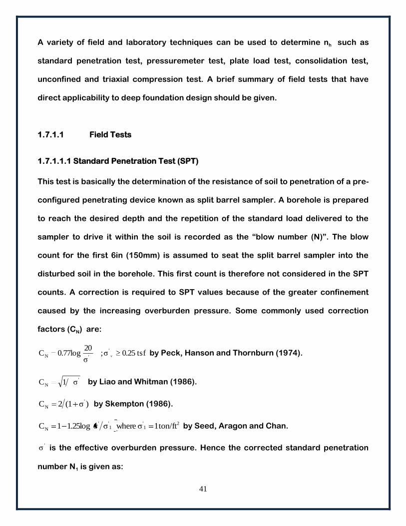
counts. A correction is required to SPT values because of the greater confinement
caused by the increasing overburden pressure. Some commonly used correction
factors (CN) are:
tsf0.25σ;σ
200.77logC
v
'
'N by Peck, Hanson and Thornburn (1974).
'
N σ1C by Liao and Whitman (1986).
)σ(12C '
N by Skempton (1986).
21'
1''
N ton/ft1σwhereσσ1.25log1C by Seed, Aragon and Chan.
'σ is the effective overburden pressure. Hence the corrected standard penetration
number N1 is given as:
42
N1=CN.NF (40)
Where NF is the field standard penetration number.
Over the years many useful correlations between N and soil parameters have been
developed. One useful correlation proposed by Scott (1981) between coefficient of
subgrade reaction (k) and corrected blow count (Ncor) is:
K(MN/m3) =18 Ncor or k(US ton/ft3) =6 Ncor (41)
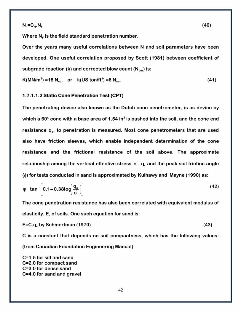
1.7.1.1.2 Static Cone Penetration Test (CPT)
The penetrating device also known as the Dutch cone penetrometer, is as device by
which a 60 cone with a base area of 1.54 in2 is pushed into the soil, and the cone end
resistance qc, to penetration is measured. Most cone penetrometers that are used
also have friction sleeves, which enable independent determination of the cone
resistance and the frictional resistance of the soil above. The approximate
relationship among the vertical effective stress 'σ , qc and the peak soil friction angle
( ) for tests conducted in sand is approximated by Kulhawy and Mayne (1990) as:
(42)
The cone penetration resistance has also been correlated with equivalent modulus of
elasticity, E, of soils. One such equation for sand is:
E=C.qc by Schmertman (1970) (43)
C is a constant that depends on soil compactness, which has the following values:
(from Canadian Foundation Engineering Manual)
C=1.5 for silt and sand C=2.0 for compact sand C=3.0 for dense sand C=4.0 for sand and gravel
'
c1
σ
q0.38log0.1tanφ

43
Trofimenkov (1974) gave the following correlations for sand and clay:
E=3qc (sand) (44)
E=7qc (clay) (45)
1.7.1.1.3 Flat Plate Dilatometer Test (DMT)
This test consists of the insertion of a flat plate 14 mm thick, 95mm wide and 220mm
long. The device has a flexible steel membrane, 60mm in diameter, located on one
face of the blade as shown in figure 1.19.
Figure 1.19 – Marchetti flat-plate dilatometer (Prakash,2004)
A measuring device is located beneath this membrane, which turns off when the
membrane starts to lift off by high-pressure nitrogen gas, and turns on at a deflection
of 1mm at the center of the membrane due to the pressure from the surrounding soil.
The pressure required to lift the membrane is Po and the pressure to cause 1mm
deflection at the center of the membrane is P1. These dilatometer readings are than
corrected to allow for offset in the measuring gauge and membrane stiffness. Using
Po and P1 the following parameters were proposed:
Material index=Id= (P1- Po)/(Po-U) (46)

44
Horizontal stress index=Kd=(Po-U)/ 'σ (47)
Dilatometer modulus=Ed=34.6(P1- Po) (48)
Where U= assumed in-situ hydrostatic water pressure.
1.7.1.1.4 Borehole Pressuremeter Test
This test involves the use of an expandable cylindrical tube placed at the bottom of a
borehole. The cylinder is then expanded under controlled conditions against the
surrounding soil. The most widely used version of pressuremeters is the Menard
(1956) pressuremeter. It is a pre-bored pressuremeter (as opposed to self bored and
full displacement pressuremeters), which consists of a pressure cell and two guard
cells. Applying air pressure to a liquid that fills the instrument expands the pressure
cell, and the test involves the measurement of the expansion of the volume of the
pressure cell. Figure 1.20 shows the variation of the pressure cell volume with
changes in the cell pressure.
Figure 1.20 – Idealized pressure-expansion curve from Menard type pre-bored pressuremeter test (Robertson, 1986)

45
Zone 1 represents the reloading portion, during which the soil around borehole is
pushed back to it’s initial state which is the state it was before drilling. Zone 2
represents a pseudoelastic zone, in which the cell volume versus the cell pressure is
practically linear. The zone 3 is the plastic zone.
For zone 2 the E of soil is given as:
(49)
Pressuremeter test results can be used to determine the at rest earth pressure
coefficient Ko, which is given by:
(50)
Pressuremeter test results are very sensitive to the conditions of the borehole
prepared before the test.
1.7.1.2 API Procedure for Developing P-Y Curves
Coefficient of subgrade modulus and the elastic modulus of soil are the main
parameters that are needed to represent soil resistance by spring elements to
capture the load-displacement characteristic of the soil.
There are several relationships that relate soil stiffness for a given drilled shaft
geometry and soil type to the soil elastic modulus. Some of these relationships are
shown in equation (51). The majority of these equations are based on experimental
studies and modifications to achieve an agreement between the units on both sides of
the equation. However there are disagreements among the results obtained, and for a
given case it is not readily apparent which equation to use to obtain the required soil
stiffness parameters.
ΔV
Δpυ)V2(1E o
'
oo
σ
pK

46
(51)
B is the shaft diameter, I is the moment of inertia of the shaft, and E is the elastic
modulus of the soil that is linearly related to the coefficient of subgrade reaction nh.
Figure 1.21 presents the variation of spring stiffness values obtained for a 6 ft
diameter shaft in medium sand with nh=22.5lb/in3 based on the proposed relations in
equation (51).
Figure 1.21 – Variation of spring stiffness with different equations.
c)(VesiEμ-1B
1.
.IE
B0.65k
12
13
s
12
1
pp
2
4
h
(Poulos)EB
0.8k sh
(Bowles)EB
1.3)to(0.8k sh
(Terzaghi)EB
0.74k sh
(Broms)EB
0.9)to(0.48k sh
Spring stiffness vs. Depth
0
10
20
30
40
50
60
70
80
90
100
0 500 1000 1500 2000 2500 3000 3500 4000
Spring stiffness (kip/ft)
De
pth
(ft
)
Vesic
Poulos
Bowles1
Bowles2
Terzaghi
Broms1
Broms2

47
The reasons for the variations in the results can be due to differences in testing
methods, the evaluation of the test results, and assumptions regarding the lateral
behavior of a deep-foundation.
As a result of an attempt to establish a more unified approach to define stiffness
characteristics of soil, experimental studies, conducted in the 1970s (Matlock, 1970;
Reese et al., 1974; Reese and Welch, 1975; Bhushan et al.1979), on the response of
pile foundations to cyclic and quasi-static lateral loads led to the development of the,
so-called, p-y curves. Different p-y relationships have been proposed for sand (Cox et
al. 1974, Reese et al. 1974), which were subsequently adopted by the American
Petroleum Institute for routine use (API 1993). The procedure for the estimation of p-
y curves for a given shaft in cohesionless soils is as follows:
Step 1: Estimate the angle of internal friction (υ ) and unit weight (γ) for the soil.
Step 2: Calculate the following parameters:
βxtanφtanBγK1βtanxBγAKp
BKtanαsinβtanφxtanβKxtanβtanβBφβtan
tanβ
cosαφβtan
sinβxtanφkxAγp
φ2
145tanK,0.4K,α45β,φ
2
1α
4
o
8
Acd
Aoo
cr
2
Ao
Note that pcr is applicable for depths from ground surface to a critical depth xr, and pcd
is applicable below the critical depth. The value of critical depth is obtained by
plotting these two variables on a common scale. The point of intersection of these two
curves will be xr, which is shown in figure 1.22.

48
Figure 1.22 – Intersection of pcr and pcd (Reese,1974).
Step 3: Select a particular depth at which a p-y curve will be drawn. Compare this
depth with the critical depth obtained in step 2 and then find the value that is
applicable. Then carry out the calculations for a p-y curve as follows. Refer to figure
1.23 for the following steps.
Figure 1.23 – Estimation of a p-y curve by the API procedure (Reese, 1974).

49
Step 4: Select an appropriate value for nh (coefficient of subgrade reaction). Calculate
the following parameters:
diameter.shaft theis B WhereCyp,xn
Cy,
y
pC
my
pn,
yy
ppm,
80
3By,pAp,
60
By,pBp
1/n
1)n/(n
h
k1/n
m
m
m
m
mu
mu
uc1umc1m
The constants A1 and B1 are selected from table 1.4, which was tabulated from curves
provided by Reese et at. (1974).
Table 1.4 – Values for coefficients A1 and B1 (Reese et al.1974)
x/B A1 B1
Static Dynamic Static Dynamic
0 2.85 0.77 2.18 0.5
0.2 2.72 0.85 2.02 0.6
0.4 2.6 0.93 1.9 0.7
0.6 2.42 0.98 1.8 0.78
0.8 2.2 1.02 1.7 0.8
1 2.1 1.08 1.56 0.84
1.2 1.96 1.1 1.46 0.83
1.4 1.85 1.11 1.38 0.86
1.6 1.74 1.08 1.24 0.86
1.8 1.62 1.06 1.15 0.84
2 1.5 1.05 1.04 0.83
2.2 1.4 1.02 0.96 0.82
2.4 1.32 1 0.88 0.81
2.6 1.22 0.97 0.85 0.8
2.8 1.15 0.96 0.8 0.78
3 1.05 0.95 0.75 0.72
3.2 1 0.93 0.68 0.68
3.4 0.95 0.92 0.64 0.64
3.6 0.94 0.91 0.61 0.62
3.8 0.91 0.9 0.56 0.6
4 0.9 0.9 0.53 0.58
4.2 0.89 0.89 0.52 0.57
4.4 to 4.8 0.89 0.89 0.51 0.56
5 and more 0.88 0.88 0.5 0.55

50
Step 5: a. Locate the yk on the y-axis in Figure 1.23. Substitute this value of yk as y in
and determine the corresponding p value. This p value will define the k point. Join
point k with origin O.
b. Locate the point m for the values of ym and pm from the equations in step 4.
c. Plot the parabola between the k and m.
d. Locate the point u from the values of yu and pu from the equations step4.
e. Join points m and u with a straight line.
Step 6: Repeat the above procedure for various depths to obtain p-y curves at each
depth below the ground.
With the API procedure, the soil stiffness that is needed to develop a spring model is
obtained. Before proceeding with the development of the model, one needs to divide
the drilled shaft into hypothetical intervals. The p-y curves are obtained at these
intervals along the depth of the shaft. The unit of p is force/unit depth. Thus, if a
certain interval of soil is to be represented by a spring that has non-linear load
displacement relation defined by the p-y curve, the value of p has to be multiplied by
the depth of the interval. Thus, the soil is represented by a spring with non-linear
properties.

51
1.8 SSI Modeling of Deep Foundations
The theories developed so far, have approached the problem of analyzing a laterally
loaded shaft by considering certain aspects of the problem and ignoring certain
others. Because of the highly indeterminate nature of the problem, any suggested
approach is bound to have deficiencies. In order to include as much SSI
characteristics as possible within the analysis, finite element methods will be
employed. The finite element modeling will start with the spring analogy of the
laterally loaded deep foundations and then develop into more refined and evolved
continuum models where soil continuity as well as the various aspects of the soil
structure interaction such as surface friction and soil selfweight deformation will be
included. The software that will be used to develop the finite element models is
ABAQUS version 6.4. ABAQUS consists of two main analysis modules which are:
ABAQUS/Standard and ABAQUS/Explicit. ABAQUS/Standard is a general-purpose
analysis module that can solve a wide range of linear and nonlinear problems.
ABAQUS/Explicit is a special-purpose analysis module that uses an explicit dynamic
finite element formulation. It is suitable for short, transient dynamic events and is also
very efficient for highly nonlinear problems involving changing contact conditions.
1.8.1 Finite Element Modeling in SSI In case of drilled shafts, certain other soil parameters also take role in resisting
lateral loads. As an addition to load-displacement characteristics of the shaft and the
soil; behavior and parameters that are unaccounted for in the previous theories and
models such as 1) shear coupling between the soil layers, 2) soil-structure interface
friction, 3) shaft confinement due to selfweight deformations, 4) poissons ratio of the

52
soil and 5) support condition modeling, can be included within a finite element model.
The finite element method provides the most powerful means for conducting SSI
analyses.
Figure1.24 shows the loading and the forces generated on a deep foundation that is
subject to bending and axial loadings.
Figure 1.24 – Lateral loading and resistance components on a drilled shaft (Chen) Many researchers have used FEA in the past. Yegian and Wright (1973) implemented
a finite element analysis with a radial soil-pile interface element that described the
nonlinear lateral pile response of single piles and pair of piles subjected to static
loading. Based on work by Kausel et al. (1975), Blaney et al. (1976) used a finite
element formulation with a consistent boundary matrix to represent the free-field,
subjected to both pile head and seismic base excitations and derived dynamic pile
stiffness coefficients as a function of dimensionless frequency. Desai and Appel
(1976) presented a three-dimensional finite element solution with interface elements

53
for the laterally loaded pile problem. Randolph and Wroth (1978) modeled the linear
elastic deformation of axially-loaded piles. Kuhlemeyer (1979a) offered efficient static
and dynamic solutions for lateral soil-pile elastic response; Kuhlemeyer (1979b) used
a finite element model of dynamic axially loaded piles to verify Novak’s (1977) solution
and a simplified method presented by the author. Angelides and Roesset (1981)
incorporated equivalent linearization scheme to model nonlinear soil-pile response.
Randolph (1981) derived simplified expressions for the response of single piles and
groups from a finite element parametric study. Kay et al. (1983) promoted a site-
specific design methodology for laterally loaded piles consisting of pressuremeter
test data as input to an axisymmetric finite element program. Lewis and Gonzalez
(1985) compared field test results of drilled piers to a 3-D finite element study that
included nonlinear soil response and soil-pile gapping. Trochianis et al. (1988)
investigated nonlinear monotonic and cyclic soil-pile response in both lateral and
axial modes with a 3-D finite element model of single and pairs of piles, incorporating
slippage and gapping at the soil-pile interface. They deduced a simplified model
accommodating pile head loading only. Koojiman (1989) described a quasi-3-D finite
element model that substructured the soil-pile mesh into independent layers with a
Winkler type assumption. Brown et al. (1989) obtained p-y curves from 3-D finite
element simulations that showed only fair comparison to field observations. Bhowmik
and Long (1991) devised 2-D and 3-D finite element models that used a bounding
surface plasticity soil model and provided for soil-pile gapping. Brown and Shie
(1991) used a 3-D finite element model to study group effects on modification of p-y
curves.

54
1.8.2 Finite Element Analysis Overview Finite element analysis is a method for numerical solution of field problems and a field
problem is the spatial distribution of one or more dependent variables. The region of
interest for the distribution of this field is mapped or geometrically defined by nodes
and than discretized into and represented by “finite” geometric units in which the
field variable is allowed to vary from node to node in a way described by a polynomial
function. The location of the nodes is the locations where the value of field of interest
is sought. The units, which are defined by “nodes”, are called the “elements”, and the
particular assembly of these elements is called the mesh. The algebraic equations
within these elements are solved for the unknown field quantities at the nodes. The
solution procedure for a time-independent FEA can be summarized as:
1. Description the element behavior through matrices.
2. Assembly of the individual matrices through element connection.
3. Establishing the loading and boundary conditions.
4. Determination of nodal quantities through algebraic equations created by a
system of structure matrix, loading and the boundary conditions.
5. Computation of gradients.
FEA is a necessary method for cases where the load support mechanism within a
structure is not clearly visible and an approximate representation of structural
mechanism is needed in order to analyze structural behavior. Since FEA is a
methodology to model and analyze any type of physical problem, there are many
different elements that are configured for different applications. However, these
elements are not randomly configured and every element can be defined by certain
characteristics, which can be defined by:

55
Family that the element belongs to.
Degrees of freedom (related to the element family) of the element.
Number of nodes of the element.
Formulation of the element.
Integration within the element.
In SSI analysis of deep foundations, the family of elements shown in figure 1.25 has
been excessively used.
Figure 1.25 – Element families that are used in the finite element models for the SSI analysis of deep foundations.
The degrees of freedom (dof) are the fundamental variables calculated during the
analysis. The d.o.f refers to the number of independent displacement modes the
element can display. For a stress/displacement simulation the degrees of freedom are
the translations. For shell and beam elements, the rotations at each node as well as
the displacement constitute the d.o.f. Displacements, rotations, and the other
degrees of freedom are calculated only at the nodes of the element. At any other
point in the element, the displacements are obtained by interpolating from the nodal
displacements. Generally the number of nodes used in the element determines the
interpolation order. Figure 1.26 shows the interpolation associated with continuum
elements.
Spring elements

56
Figure 1.26 – Order of interpolation within the elements.
An element's formulation refers to the mathematical theory used to define the
element's behavior. All of the stress/displacement elements in ABAQUS are based on
the Lagrangian or material description of behavior, which states that the material
associated with an element remains associated with the element throughout the
analysis, and material cannot flow across element boundaries.
In order to evaluate the variation of the field of interest within an element, ABAQUS
uses numerical techniques to integrate various quantities over the volume of each
element. Using Gaussian quadrature for most elements, ABAQUS evaluates the
material response at each integration point in each element. Choosing between full or
reduced integration of the element controls the integration locations within the
elements.
The FEA provides an approximate result to a complicated structural problem where
an exact analysis cannot be conducted due to the extent of the structural domain and
the variety of interactions that take place within this domain. The level of this
approximation is related to the pre-modeling assumptions, nodal meshing and
selection of elements, specifying boundary conditions and describing material
properties.

57
Solutions provided to a structural problem can be exact or approximate. An exact
solution must satisfy compatibility, equilibrium and boundary conditions.
Compatibility condition requires the displacements to be continuous and single
valued functions of position. Equilibrium condition requires that the summation of
forces and the moments that the structure is subject to be zero. Boundary conditions
include the necessary prescription of displacements and rotations at particular
points within the structure for the structure to attain the equilibrium conditions.
The satisfaction of these conditions for every point within a structure through direct
methods can only be attained for simple structures where an exact mathematical
formulation can be easily constructed. Exact solutions are known only for simple
combinations of geometry, loading and support conditions. Finite element
representation of complicated domains and interactions satisfy the equilibrium
conditions in an integral or average sense.
A geometric model becomes a mathematical model when its behavior is described or
approximated by differential equations and boundary conditions. Since the geometric
model is a discretized representation of the continuous structure, the mathematical
model is a continuous field function represented or defined by a finite number of
discretized functions that vary within the elements in a predetermined way satisfying
a certain value at the nodes. In brief, finite element analysis is method in which a field
variable is approximated by connecting simple interpolation functions, each defined
over a small region, which is called a finite element.
To interpolate is to devise a function that satisfies the prescribed conditions at a finite
number of points i.e. the nodes of an element. The prescribed conditions are the
nodal values of a field quantity. In structural engineering problems, the distribution of

58
field that is of interest is the “displacements”. The stresses within the modeled body
are based on these displacement gradients. In finite element analysis, the
interpolation function is generally a polynomial, which provides a single-valued and a
continuous field.
An interpolating polynomial with dependent variable and an independent variable x
can be written in the general form as:
T
n210
n2
n
0i
i
i
aaaaaandxxx1Xwhere
aXφorxaφ
(52)
For n=1 the interpolating polynomial is linear and for n=2 it is quadratic. The field
quantity is interpolated within each element in a piecewise fashion over a finite
element mesh. The greater the number of terms included in the approximation, the
more closely the exact solution is represented.
An alternative representation of is:
aAφwhereφNφ ii (53)
From equation (1) and (2):
1AXN (54)
A member Ni in the N row vector is called a shape function, which states the
interpolated = (x) when the corresponding i at a nodal location is unity and the
others are zero. Assembly of elements causes element nodal values e to appear in
the global vector of degrees of freedom D . Figure 1.27 shows the concepts of linear
and quadratic interpolations of the field quantities and the associated shape
functions.

59
Figure 1.27 – (a) Linear interpolation and shape functions, (b) Quadratic interpolation and shape functions.
The field quantity is interpolated in a piecewise fashion over a finite element mesh.
The interpolation takes place within an element. Thus, while varies continuously
within an element, the transition may not be continuous. The concept of continuity
among elements is defined with Cm, where m defines the degree of derivative of the
function. Thus = (x) is C0 continuous if is inter-element continuous but not the first
derivative ’, and C1 continuous if both and ’ is inter-element continuous but not ’’.
Plane and solid body elements are usually modeled by C0 elements. C1 elements on
the other hand are used to model beams, plates and shells where the nodal degrees
of freedom include rotations and the continuity of the slope is required. Figure 1.28
shows the continuity of the functions with different degrees.

60
Figure 1.28 – (a) Functions, (b) Continuity of the functions.
The linear and quadratic interpolation and the shape functions for C0 interpolation are
shown in figure 1.27. The interpolation scheme presented in this figure is the
Lagrange’s Interpolation Formula, which can be generalized with:
(55)
Where k is the number of curve fitting points, which is k=2 for linear interpolation and
k=3 for quadratic interpolation. This interpolation scheme only uses displacements,
so the slope information is not used.
1.8.3 Types of Elements Four types of finite elements have been commonly used in the FE models developed
for the SSI analysis of deep foundations.
1.8.3.1 Beam Elements
Cases in which the primary solution variables can be described as functions of
position along the beam longitudinal axis, the physical element can be described by a
beam element. For such an assumption to be reasonable, the beam must be such a
continuum that the shortest vertical distance from the beam longitudinal axis to
)x(xxx)x)(xx(x
x)(xxxx)x)(x(xN
knkkk2k1
nk21k

61
anywhere in the continuum should be very small compared to typical lengths along
the longitudinal axis.
The simplest approach to beam theory is the classical Euler-Bernoulli assumption,
that plain cross-sections initially normal to the beam’s axis remain plane. This
assumption holds when the associated shear deformations are very small compared
to bending deformations, as it is in the case of slender beams. In order for beams of
uniform material to be considered slender in ABAQUS, the smallest dimension along
the cross-section should be equal or smaller than about 1/15 of the longitudinal
dimension.
The extended version of the Euler-Bernoulli assumption is the Timoshenko beam
theory (Timoshenko, 1956) where the transverse shear deformations due to shear
strains at the cross-section are also considered. For thicker (stout) beams having
slenderness values larger than 1/15, shear flexibility becomes important and the
Euler-Bernoulli assumption does not apply, i.e. plain sections do not remain plane.
The beam elements developed to consider the shear deformations in thick beams
could also be used for slender beams where the shear deformations are not
significant. So the use of these elements for all cases covers all-basis.
1.8.3.2 Spring Elements
The load-displacement characteristics of soil are idealized by the use of spring
elements. Spring element can couple a force with a relative displacement and can be
linear or nonlinear. When the spring is associated with displacement degrees of
freedom, these variables are the force and relative displacement in the spring. Figure

62
1.27 shows the nonlinear load-displacement characteristics of the spring element,
which is obtained through p-y curves.
Figure 1.27 – Nonlinear spring force–relative displacement relationship.
1.8.3.3 Solid Elements
Solid elements are the standard elements to define a continuum. The
ABAQUS/Standard solid element library includes first-order (linear) interpolation
elements and second-order (quadratic) interpolation elements in one, two, or three
dimensions. Triangles and quadrilaterals are available in two dimensions; and
tetrahedra, triangular prisms, and hexahedra (“bricks”) are provided in three
dimensions. Modified second-order triangular and tetrahedral elements are also
provided. Figure 1.28 shows the linear and quadratic solid elements.

63
Figure 1.28 – Rectangular solid elements (a) 8 node tri-linear element with 24 d.o.f, (b) 20 node element with 60 d.o.f.(Cook, Malkus, 2004)
The eight node trilinear element has been used for the interior soil elements
(boundary soil has been defined by the infinite elements). The displacements u, v and
w for the linear element are defined by equation (56) that result in 24 d.o.f.
(56)
In terms of the shape functions, the element displacement field is:
(57)
Which can also be defined as:
(58)
The individual shape functions in the displacement field have the form:
(59)
xyzazxayzaxyazayaxaaw
xyzazxayzaxyazayaxaav
xyzazxayzaxyazayaxaau
2423222120191817
161514131211109
87654321
dNu
8abc
z)y)(cx)(b(aNi

64
1.8.3.4 Infinite Elements
Analytical modeling of unbounded domains such as the lateral load analysis of soil-
structure interaction system of deep foundations, face the problem of determining the
effective continuous media extent. Extending the finite element mesh to a far
distance, where the influence of the surrounding medium may be neglected, can
approximate the infinite medium. With this approach, boundary conditions will have to
be implemented at the terminated ends of the model mesh. However, the use of
boundary conditions not only a creates a longer execution time but also becomes
particularly problematic in dynamic analysis, where the mesh boundary could reflect
the energy back into model, where in fact it is dissipated in to the surrounding
domain. Because of these problems, a better approach is to use “infinite elements”
that are defined over semi-infinite domains. In modeling SSI models such as laterally
loaded deep foundations, infinite elements can be used at the termination of the
model defined by solid elements.
ABAQUS provides first- and second-order infinite elements that are based on the
work of Zienkiewicz et al. (1983) for static response and of Lysmer and Kuhlemeyer
(1969) for dynamic response. The infinite elements shown in figure 1.29 are used in
conjunction with standard finite elements, which model the area around the region of
interest, with the infinite elements modeling the far-field region.

65
Figure 1.29 – An infinite solid element. 1.8.4 Inherent Problems Associated with Finite Elements For the linear, fully integrated elements there is a problem caused called the shear
locking. Shear locking causes the elements to be too stiff in bending. Figure 1.30
shows the distortions in a structure subject to pure bending. Lines initially parallel to
the horizontal axis take on constant curvature, and lines through the thickness
remain straight, the angle between the horizontal and vertical lines remains at 90°
meaning that the plane sections will remain plane as long as the shear deformations
can be disregarded.
Figure 1.30 – Deformed shape under pure bending.
Figure 1.31 shows the deformed shape of the linear fully integrated continuum
element used to model the structure under pure bending. The edges of a linear
element are unable to curve; therefore, if the small piece of material is modeled using
a single element, its deformed shape will be like a trapezoid.

66
Figure 1.31 – Deformed shape of the fully integrated element.
The dotted lines that pass through the integration points are plotted. It is apparent
that the upper line has increased in length, indicating that the direct stress in the 1-
direction is tensile. Similarly, the length of the lower dotted line has decreased,
indicating that the stress is compressive. The length of the vertical dotted lines has
not changed (assuming that displacements are small); therefore, the stresses along
the 2-direction at all integration points are zero. All this is consistent with the
expected state of stress of a small piece of material subjected to pure bending.
However, at each integration point the angle between the vertical and horizontal
lines, which was initially 90°, has changed. This indicates that the shear stress, at
these points is nonzero. This is incorrect because the shear stress in a piece of
material under pure bending is zero. This parasitic shear stress arises because the
edges of the element are unable to curve. Its presence means that strain energy is
creating shearing deformation rather than the intended bending deformation, so the
overall deflections are less because the element is too stiff. One way to overcome this
problem is to decrease the number of integration points within the element in order to
make the shear strains ineffective in creating extra stiffness. The so-called reduced-
integration elements as shown in figure 1.32 use one fewer integration point in each
direction than the fully integrated elements. Reduced-integration, linear elements
have just a single integration point located at the element's centroid.

67
Figure 1.32 – Integration points in reduced integration elements.
However, linear reduced-integration elements tend to be too flexible because they
suffer from their own numerical problem called hourglassing. Consider a single
reduced-integration element modeling a small piece of material subjected to pure
bending
Figure 1.33 – Reduced integration linear element. Neither of the dotted visualization lines has changed in length, and the angle between
them is also unchanged, which means that all components of stress at the element's
single integration point are zero. This bending mode of deformation is thus a zero-
energy mode because no strain energy is generated by this element distortion. The
element is unable to resist this type of deformation since it has no stiffness in this
mode. In coarse meshes this zero-energy mode can propagate through the mesh,
producing meaningless results. Thus care must be taken when using reduced
integration elements to model structures under bending, and sufficient number of
elements must be used to generate enough integration points along the depth of the
structure subjected to bending. The problems associated with the finite elements
should be taken into consideration in developing a finite element model for SSI of
deep foundations or in general, developing a FEM for any type of application. In order

68
to overcome the problems associated with the shear locking, linear-reduced
integration elements can used to model the shaft. In order to prevent hourglassing,
multiple layers of elements can be used along the cross-section of the shafts. Since
the soil elements are mostly under compression, linear-full integration elements can
be used to model the soil continuum.
1.9 Time Integration Procedures
The numerical problem defined within the ABAQUS model can be conducted either by
ABAQUS/Standard or ABAQUS/Explicit. For both the explicit and the implicit time
integration procedures, equilibrium is defined in terms of the external applied forces,
P, the internal element forces, I, and the nodal accelerations:
(60)
M is the mass matrix. Both procedures solve for nodal accelerations and use the
same element calculations to determine the internal element forces. The biggest
difference between the two procedures lies in the manner in which the nodal
accelerations are computed.
ABAQUS/Standard uses automatic incrementation based on the full Newton iterative
solution method. Newton's method seeks to satisfy dynamic equilibrium at the end of
the increment at time t+ t and compute displacements at the same time. The time
increment, t, is relatively large compared to that used in the explicit method because
the implicit scheme is unconditionally stable. For a nonlinear problem each increment
typically requires several iterations to obtain a solution within the prescribed
tolerances. Each Newton iteration, solves for a correction, cj, to the incremental
IPuM..

69
displacements uj. Each iteration requires the solution of a set of simultaneous
equations:
(61)
The solution for such equations takes long time for large models, or models with
complex contact interactions. The effective stiffness matrix Kj is a linear combination
of the tangent stiffness matrix and the mass matrix for the iteration. The iterations
continue until force residual, displacement correction, are within the prescribed
tolerances. For a smooth nonlinear response Newton's method has a quadratic rate
of convergence. However, if the model contains highly discontinuous processes,
such as contact and frictional sliding, quadratic convergence may be lost and a large
number of iterations may be required. In some cases convergence may not be
possible using the implicit method
Complex frictional contact conditions conditions and other discontinuous event are
formulated more easily using an explicit dynamics method than using an implicit
method and can be enforced on a node-by-node basis without iteration. The nodal
accelerations can be adjusted to balance the external and internal forces during
contact. The most important feature of the explicit method is the lack of a global
tangent stiffness matrix, which is required with implicit methods. Since the state of
the model is advanced explicitly, iterations and tolerances are not required.
ABAQUS/Explicit uses a central difference rule to integrate the equations of motion
explicitly through time, using the kinematic conditions at one increment to calculate
the kinematic conditions at the next increment. At the beginning of the increment the
program solves for dynamic equilibrium, which is stated in equation (60). The
accelerations at the beginning of the current increment (time t) are calculated as:
j
..
jjjjj uMIPcK

70
(62)
The accelerations are integrated through time using the central difference rule,
which calculates the change in velocity assuming that the acceleration is constant.
This change in velocity is added to the velocity from the middle of the previous
increment to determine the velocities at the middle of the current increment:
(63)
The velocities are integrated through time and added to the displacements at the
beginning of the increment to determine the displacements at the end of the
increment:
(64)
Thus, satisfying dynamic equilibrium at the beginning of the increment provides the
accelerations. Knowing the accelerations, the velocities and displacements are
advanced “explicitly” through time. The term “explicit” refers to the fact that the state
at the end of the increment is based solely on the displacements, velocities, and
accelerations at the beginning of the increment. This method integrates constant
accelerations exactly. For the method to produce accurate results, the time
increments must be quite small so that the accelerations are nearly constant during
an increment. Since the time increments must be small, analyses typically require
many thousands of increments. However, each increment is simple because there are
no simultaneous equations to solve. Most of the computational expense lies in the
element calculations to determine the internal forces of the elements acting on the
nodes. The element calculations include determining element strains and applying
(t)
1(t)
..
I).(P(M)u
(t)
..(t)Δt)(t
2
Δtt
.
2
Δtt
.
u2
ΔtΔtuu
2
Δtt
.
Δt)(t(t)Δt)(t uΔtuu

71
material constitutive relationships (the element stiffness) to determine element
stresses and internal forces.
1.10 Soil Modeling
Specification of the material behavior is an important task in developing a SSI model.
Soil is a mixture of unbonded granular material of mineral and organic origin. It is
generally referred to as gravel, sand, silt, clay or a mixture of these. The mechanical
behavior of soils are very complicated due to the fact that unlike the properties of
most engineering materials, deformational and strength characteristics are greatly
affected by the factors such as soil texture, density, water content, degree of void
saturation, loading rate, confining pressure and stress history. The mathematical
characterization of the mechanical behavior of soil should ideally be based on
consideration of the individual particles and their interaction. One such approach has
been proposed by Harr (1977) in which the overall deformation characteristics are
studied on a microscopic level of soil particle interaction. However, such an
approach creates problems of extremely complex nature. Thus an exact
characterization of soil for any given condition is a very hard task to accomplish. On a
large scale when the mass of soil under consideration is large which is usually the
case, the granular nature of the soil can be approximated by a continuous nature and
can be analyzed within the framework of continuum mechanics. Soil mechanics,
which is treated within the framework of such an idealization, is therefore a branch of
mechanics of solid.
Soil-mechanics problems are considered within the context of deformations, stability
and viscoelasticity. The deformations within the soil are a matter of load-
displacement characteristics of the soil mass when no failure of the soil is involved.

72
The stability however, is a matter of ultimate failure of the soil. Time related long term
settlement and consolidation problems constitute viscoelastic problems.
Traditionally the deformations have been considered elastic and have been treated
by Hooke’s law. The plastic behavior on the other hand has been considered as
perfect plasticity i.e. the strain hardening is overlooked. These idealizations
regarding the pre-failure and failure states of soil have been necessary due to a
complicated soil nature.
The development of the modern theory of soil plasticity was strongly influenced by
metal plasticity, which dates back to 1864 when Tresca introduced the first yield
criterion for ductile metals, which is known as maximum shear stress criterion. In
1913 Von Mises introduced a new yield criterion, which is known as distortion energy
criterion. The first major advance in the extension of metal plasticity to soil plasticity
was made in the paper “Soil mechanics and plastic analysis or limit design” by
Drucker and Prager(1952). In this paper, the authors extended the Mohr-Coulomb
criterion to three dimensional soil mechanics problems. Drucker interpreted the
Mohr-Coulomb criterion as a modified Tresca as well as an extended von Mises yield
criterion. The yield criterion obtained by Drucker and Prager is now also known as
Drucker-Prager model. In 1957 another important advance was made in the paper
“Soil mechanics and work hardening theories of plasticity” by Drucker et.al where the
concept of work-hardening plasticity was introduced into soil mechanics. However,
the soil models used in this research will be elastic-perfectly plastic.

73
1.10.1 Mohr-Coulomb Yield Criterion In cases where the yield strength depends on hydrostatic pressure, Tresca and Von
Mises fails to completely portray the failure state of granular materials such as soil
since both criteria are developed for metals whose yield strength is insensitive to
hydrostatic pressure.
The Mohr criterion (1900) states that materials fail not because of from either
maximum normal or shear stress alone, but a critical combination of normal stresses
and shear stresses. Thus the relationship between normal stress and shear stress on
a failure plane is non-linear and can be expressed as:
=f( ). (60)
For most soil mechanics problems it is generally assumed that plastic flow occurs
when on any plane at any point in a mass of soil, the shear stress (τ) reaches an
amount that depends linearly upon the cohesion stress (c) and the normal stress (σ)
provided σ is a compressive stress and it is sufficient to approximate the shear stress
on the failure plane as a linear function of the normal stress (Coulomb, 1776), which
can be expressed as:
τ = c + tanυ (61)
Equation (61) is known as the Mohr-Coulomb criterion, which is a linear
approximation of Mohr criterion and defines the effect of hydrostatic pressure in soil
strength. The angle φ is the angle of internal friction of the soil, which is assumed to
be constant for a wide range of hydrostatic pressures. The constants c and υ are
parameters, which characterize the total resistance of the soil to shear. A soil
medium in which cohesion is absent (c=0) is called a cohesionless soil and one in
which the internal friction is absent =0 a purely (ideally) cohesive soil. Tresca’s yield

74
criterion, which applies to ductile metals, corresponds to the particular case of
Coulombs yield criterion when there is no internal friction. In other words, the Tresca
yield criterion in metals can be alternatively represented with c=k and =0 where k is
the shear yield stress for metals.
According to Mohr’s criterion, intermediate principal stress, 2 ( 1 2 3), has no
influence on the failure criterion. In terms of principal stresses, the failure condition
represented by equation (61) can be written as:
(62)
In the principal stress space, the Mohr-Coulomb criterion represents an irregular
hexagonal pyramid as shown in figure 1.34. The failure surface in the meridian planes
is straight lines and its deviatoric trace is an irregular hexagon as shown in figure
1.35.
Figure 1.34 – Mohr-Coulomb criterion in principal stress space.
ccosφsinφσσ2
1σσ
2
13131

75
Figure 1.35 –Trace of Mohr-Coulomb failure surface in the deviatoric planes.
In connection with its use for soils, the Mohr-Coulomb failure criterion has certain
shortcomings. First, it assumes that the intermediate principal stress has no influence
on failure and second, the failure surface has singularities, which creates difficulties
in numeric analysis such as FEA of SSI. Thus attempts have been made to generalize
the criterion by incorporating hydrostatic dependence for applications to soil media.
1.10.2 Drucker-Prager Yield Criterion 1.10.2.1 Extended Tresca Criterion
On the basis of the Tresca criterion, Drucker (1953) proposed an extended tresca
criterion, which can be written as:
(63)
k and are material constants to be determined experimentally. In the principal
stress space, the failure surface corresponding to the extended Tresca criterion is a
right-hexagonal pyramid whose deviatoric cross-section is a regular hexagon. Here
321133221 σσσαkσσ2
1,σσ
2
1,σσ
2
1max

76
as in Mohr-Coulomb criterion, the extended Tresca failure surface has corners, and
therefore it is not mathematically convenient to use in three-dimensional numeric
analysis. Figure 1.36 shows the yield surface of the extended Tresca on the
deviatoric plane.
Figure 1.36 – Section of the yield surface on the deviatoric plane.
1.10.2.2 Extended von Mises Criterion
The second extended criterion, which was developed by Drucker and Prager as a
modification of the von Mises model, is known as the extended von Mises criterion,
which can be written as:
(64)
The parameters k and can be determined from triaxial tests.
The extended von Mises criterion failure surface in the principal stress space is
shown in figure 1.37. This surface is a right circular cone with the hydrostatic axis as
its axis. This failure surface can be looked upon as a smooth Mohr-Coulomb surface
2
31
2
23
2
12
2
13
2
32
2
212
3212
σσσσσσσσσ6
1J
whereσσσαkJ

77
or as an extension of the von Mises surface for hydrostatic pressure dependent
materials such as soils.
Figure 1.37 – Drucker-Prager yield criterion in principal stress space.
Since no singularities exist in the failure surface defined by the extended von Mises
criterion, it is mathematically convenient to use in three-dimensional applications
such as SSI modeling with FEM. The effect of hydrostatic pressure on the soil
strength is accounted for in this criterion and unlike the Mohr-Coulomb criterion, the
influence of the intermediate principal stress is considered.
For a given case of limit strength analysis of soil case where the extended von Mises
and the Mohr-Coulomb criteria are expected to give identical results, the following
equations correlate the extended von Mises and Coulomb criterion parameters:
(65)
Due to its mathematical convenience, the Drucker-Prager criterion will be employed
as a smooth generalization of the Mohr-Coulomb failure surface in three-dimensional
analysis.
22 12tan9
3ck
12tan9
3tanα

78
1.10.3 Friction and Dilatation in Soils and Lade Criterion Most cohesionless can be considered as frictional-dilating materials. The shearing
resistance of a cohesionless soil is contributed by two actions: (1) The frictional
action that is controlled by the mineral and surface characteristics of soil particles
and (2) The dilating action, which is dependent on the particle packing conditions.
The frictional action dissipates external energy by generating heat through relative
particle movement, the dilating action changes external work into potential energy
through the re-adjustment of the particles. Thus the angle of internal friction of a
cohesionless soil is composed of two parts that is related to two different forms of
energy response.
Thus at a given relative density and level of confining stress a coarse-grain soil will
have not one but two values of υ, one corresponding to the peak strength ( peak) and
the other, smaller value corresponding to the constant-volume strength ( cv). The
relationship between peak and cv is commonly expressed as:
peak= cv + d (66)
d is called the dilatancy angle and defines the component of shear strength that
occurs due to the phenomenon of dilatancy.
Conceptually, cv reflects the basic, inherent, lower-bound strength of a soil and is
primarily a function of the shape, size, gradation and mineralogy of the soil particles
(Kulhawy and Mayne 1990). Figure 1.38 shows the Mohr’s criterion, where the
dependence of the friction angle on confining stress is depicted:

79
Figure 1.38 – Variation of angle of friction with normal effective stresses.
For common quartz sands, cv is typically in the range of 30° to 33° (Kulhawy and
Mayne 1990). On the other hand, d represents additional frictional strength that is not
present all the time but can develop from soil particle interlocking under certain
conditions of confining stress and relative density (Kulhawy and Mayne 1990). In
general, d increases with increasing relative density and/or decreasing confining
stress and can vary from 0° to more than 10° (Kulhawy and Mayne 1990). Thus
dilatancy, when and where present, can add significantly to the apparent friction
angle of a coarse-grain soil. Note, however, that no matter how large the dilatancy
contribution may be under small-strain conditions it can always be made to
"disappear" by straining the soil further. This is because additional strain always
causes the soil particles to rearrange themselves into an arrangement in which
particle-interlocking effects are minimized.
Previously presented failure criteria have one common shortcoming that neither of
them accounts for the change in friction angle with hydrostatic pressure. The original
Mohr criterion relates shear stresses and normal stresses on a failure plane and

80
makes no mention of linearity i.e. a constant angle of friction . The Mohr-Coulomb
criterion is an approximation of the general Mohr criterion, which states a linear
relation between the shear and normal stresses, which is sufficient for a limited range
of hydrostatic pressures. Figure 1.39 shows the variation in friction angle of sands
with different void ratios under different confining pressures by Marachi (1969).
It is seen that for high confining pressures the friction angle converges to a single
value.
Figure 1.39 – Variation of friction angle with confining pressure. (Marachi, 1969)
The curvature of the failure envelope i.e. the variation of the friction angle with
confining pressures has been considered in a model by Lade (1977). Lades criterion
accounts for most of the strength characteristics such as the, hydrostatic pressure
sensitivity, effect of the intermediate principal stress and the non-circular trace on
the deviatoric plane.
The inclusion of the variation of friction angle with confining pressures is becoming
important in vertical capacity analysis of foundations. Examples include bearing

81
capacity of shallow foundations (Vesic 1975), deep foundations in general (Kulhawy
1984) shallow foundations (Horvath 2000a).
However, the variation of friction angle with confining pressure will not be considered
in this research, and a single friction angle value will be used for the finite element
models developed.
1.11 Contact Modeling
Modeling of SSI involves contact between two separate bodies, namely the drilled
shaft and the surrounding soil. The interaction between contacting surfaces consists
of two components: one normal to the surfaces and one tangential to the surfaces.
The tangential component consists of the relative motion (sliding) of the surfaces and
frictional shear stresses. The general aim of contact simulations is to identify the
areas on the surfaces that are in contact and to calculate the contact pressures
generated.
In a finite element analysis, contact conditions are a special class of discontinuous
constraint, allowing forces to be transmitted from one part of the model to another.
The constraint is discontinuous because it is applied only when the two surfaces are
in contact. When the two surfaces separate, no constraint is applied. The analysis has
to be able to detect when two surfaces are in contact and apply the contact
constraints accordingly. Similarly, the analysis must be able to detect when two
surfaces separate and remove the contact constraints.
ABAQUS/Standard provides two formulations for modeling the interaction between
two deformable bodies. The first is a small-sliding formulation in which the contacting
surfaces can undergo only relatively small sliding relative to each other but arbitrary

82
rotation of the surfaces is permitted. The second is a finite-sliding formulation where
separation and sliding of finite amplitude and arbitrary rotation of the surfaces may
arise.
What constitutes “small sliding” is often difficult to define, but a general guideline to
follow is that problems where a point contacting a surface does not slide more than a
small fraction of a typical element dimension can use the “small-sliding”
approximation. The relative surface motion in the case of a laterally loaded drilled
shaft falls under the small-sliding category.
The modeling for the behavior normal to the surfaces is such that the contact
constraint is applied in ABAQUS when the clearance between two surfaces becomes
zero and the contact pressure is applied. The pressure-clearance variation in contact
simulations is defined by hard contact criteria i.e. the surfaces separate when the
contact pressure between them becomes zero or negative, and the constraint is
removed. Figure 1.40 shows the variation of pressure with clearance as defined by
hard contact criteria.
Figure 1.40 – Hard contact definition.

83
When surfaces are in contact, they usually transmit shear as well as normal forces
across their interface. Thus, the analysis may need to take frictional forces, which
resist the relative sliding of the surfaces, into account. Coulomb friction is a common
friction model used to describe the interaction of contacting surfaces.
The model characterizes the frictional behavior between the surfaces using a
coefficient of friction, . The tangential motion is zero until the surface traction
reaches a critical shear stress value, which depends on the normal contact pressure,
according to the following equation:
(67)
is the coefficient of friction and p is the contact pressure between the two surfaces.
Two contacting surface can carry shear stresses up to a certain magnitude across
their interface before they start sliding relative to each other. The Coulomb friction
model defines this critical shear stress as τcrit at which the sliding of the surfaces start
as fraction of the contact pressure, p, between the surfaces. This constant of fraction
μ is known as the coefficient of friction.
The basic model assumes isotropic friction and for the case of soil-structure surface
interaction this can be assumed to be the case. In 3-D there are 2 orthogonal
components of shear stress τ1 and τ2 along the interface of the two contacting
surfaces.
The model assumes that no relative motion occurs if equivalent shear stress is less
than the critical shear stress:
τeq = (τ12
+ τ22)0.5 (68)
By default the condition of no relative motion is approximated by stiff relative elastic
behavior. The stiffness is chosen such that the relative motion from the position of

84
zero shear stress is bounded by a value γcrit, by default this value is set to 0.5% of the
average length of all contact elements in the model.
There are two ways to define the basic Coulomb friction model. The first way is to
define the friction coefficient as a function of the slip rate, contact pressure and the
temperature.
The second way is to specify the static and kinetic friction coefficients directly and
define the exponential decay from static value to kinetic value. Figure 1.41 shows the
friction models. Experimental data shows that the friction coefficient that opposes the
initiation of slipping from a sticking condition is different from the friction coefficient
that opposes slipping. The former is referred to as the static friction coefficient and
the latter is the kinetic friction coefficient. The static friction coefficient corresponds
to the value given at zero slip-rate and the kinetic friction coefficient corresponds to
the value given at the highest slip-rate. The transition between the static and kinetic
friction is defined by the values given at intermediate slip rates. These coefficients
can be functions of contact pressure, temperature and field variables.
Figure 1.41 – Friction models. The amount and rate of relative motion between the contact surfaces and the affect of
temperature on the friction constants can be ignored in the case soil structure
p=normal force
μ.pτcritical
k
s
crit
a) Coulomb friction model
e
q
eqcγd
ksk )eμ(μμμ
b) Exponential decay friction model

85
interaction. Deformations and loading rates large enough to take into consideration
will most likely produce cases that are beyond the design strength of the deep
foundation. Also in the case of soil structure interaction, the affect of the ambient
temperature on the friction constant can also be ignored.

86
REFERENCES
1. ABAQUS Standard/Explicit Manuals versions 6.3&6.4
2. Anderson, Townsend. (2002) “A Laterally Loaded Pile Database”. Deep Foundations 2002: An International Perspective on Theory, Design, Construction, and Performance pp. 262-273
3. Baker (1993). “Use of Pressuremeter in Mixed Highrise Foundation Design”.
Design and Performance of Deep Foundations: Piles and Piers in Soil and Soft Rock pp. 1-13
4. Boulanger, Hutchinson, Chai, Idriss (2004). "Estimating Inelastic
Displacements for Design: Extended Pile-Shaft-Supported Bridge Structures” Earthquake Spectra, Vol. 20, No. 4, pp. 1081-1094.
5. Bowles (1997). “Foundation Analysis and Design 5th Edition” MacGraw-Hill
Companies
6. Briaud, Buchanan (2000) “Introduction to Soil Moduli”.
7. Briaud, L.L., Smith, T.D. Tucker, L. (1985). "Pressuremeter Design Method for Laterally Loaded Piles," Proceedings of the XI International Conference on Soil Mechanics and Foundation Engineering, San Francisco, CA, U.S.A.,
8. Briaud, Johnson, Stroman (1984). “Lateral Load Test of an Aged Drilled Shaft”
Laterally loaded deep foundations: Analysis and performance, STP 835 pp. 172-181
9. Britto, Gunn, (1987) Critical State Soil Mechanics Via Finite Elements Ellis
Horwood Limited
10. Chen, Liu (1990). “Development in Geotechnical Engineering 52 -Limit Analysis and soil plasticity” -Elsevier Publishing
11. Chen, Mizuno (1990) “Developments in geotechnical engineering53 -Nonlinear
Analysis in Soil Mechanics Theory and Implementation”- Elsevier Publishing
12. Chen (1975) “Development in Geotechnical Engineering 7 -Limit Analysis and soil plasticity”- Elsevier Publishing
13. Choi, Oh, Kwon, Kim. (2002) “A Numerical Analysis for Axial and Lateral
Behavior of Instrumented Steel Pipe Piles”. Deep Foundations 2002: An International Perspective on Theory, Design, Construction, and Performance pp. 289-304

87
14. Cook, Malkus, Plesha, Witt (2002). “Concepts and Applications of Finite Element Analysis 4th Edition” John Wiley and Sons Inc.
15. Dameron, Arzoumanidis, Bennett, Malik (1999). “Seismic Analysis and
Displacement Based Evaluation of the Brooklyn-Queens Expressway”.
16. Das (1999) “Principles of Foundation Engineering 4th edition” PWS Publishing
17. Dessai, Abel (2002). “Introduction to Finite Element Modeling”. CBS Publishers & Distributers
18. Duggal, Bohinsky, Chu. (1989) “Comparative Performance of Two Pile Types”
Foundation Engineering, pp. 943-956
19. Habigaghi, K. and Langer, J.A. (1984). “Horizontal Subgrade Modulus of Granular Soils”. Laterally loaded deep foundations: Analysis and performance, STP 835 pp. 21-34
20. Horvath, (1984). “Simplified Elastic Continuum Applied to the Laterally Loaded
Pile Problem”. Laterally loaded deep foundations: Analysis and performance, Laterally loaded deep foundations: Analysis and performance, STP 835 pp. 229-238
21. Horvath J.S. (2002) “Soil-Structure Interaction Research Project:Basic SSI
Concepts and Applications Overview” Report No. CGT-2002-2
22. Huang, Ye, Tang. (2002) “Dynamic Coupled Analysis for Earthquake Response of Pile Foundations”. Deep Foundations 2002: An International Perspective on Theory, Design, Construction, and Performance pp. 396-404
23. Kappos, Sextos (1999) “Effect of Foundation Type and Compliance on Seismic
Response on RC Bridges”. Journal of bridge engineering, Vol.6, No.2, March 2001.
24. Kulhawy. (2002) “Observations on Some Shortcomings in Foundation Analysis
and Design”. Deep Foundations 2002 (GSP 116), pp.1-5.
25. Kulhawy, Cushing.(2002) “Drained Elastic Behavior of Drilled Shafts in Cohesionless Soils”. Deep Foundations 2002: An International Perspective on Theory, Design, Construction pp. 22-36
26. Kulhawy, Agaiby, Trautmann (1996) "On large scale model testing of laterally
loaded drilled shafts in sand " Geotechnical Testing Journal , vol.v19., no.n1., pp.pp32-40.
27. Kulhawy, F. H. (1991). “Drilled shaft foundations , Foundation engineering
handbook”.

88
28. Kumar, Kort, Hosin, and Chong (2004) “Lateral Load Tests on Small Diameter Drilled Piers”
29. Kumar, Alizadeh (2002). “Lateral Load-Deflection Response of Single Piles in
Sand”.
30. Kort, Kumar, Hosin, Ng (2002) “Lateral Load Tests on Small Diameter Drilled Piers”.
31. Lin,Yang, Juang, Lee (2000). “Analysis of Laterally Loaded Piles in a Two-
Layered Elastic Medium”.
32. Lee, Kane, Bennett, Drumm (1989) “Investigation and Modeling of Soil-Structure Interface Properties”
33. Lee (1991) “Discrete Layer Analysis of Laterally Loaded Piles”.
34. Long, Reese (1984). “Testing and Analysis of Two Offshore Drilled Shafts Subjected to Lateral Loads”. Laterally loaded deep foundations: Analysis and performance, STP 835 pp. 215-228
35. Luna, Jadi (1998) “Determination of Dynamic Soil Properties Using Geophysical
Methods”.
36. Macklin, Nelson, Chou (1993) “A Lateral Load Test on Seven Foot Diameter Caissons”.
37. Maharaj (1997)“Load-Deflection Response of Laterally LoadedSingle Pile by
Nonlinear Finite Element Analysis”.
38. Matlock, Reese, (1960). Generalized Solutions for laterally Loaded Piles, Journal of the Soil Mechanics and Foundations Division, ASCE, Vol.86, No SM5, Proc.Paper 2626, pp.63-91
39. Motan, Gabr. (1989) “A Flat-Dilatometer Study of Lateral Soil Response.”
40. Neate (1983) “Augered Cast in Place Piles”.
41. Neely (1979) “Bearing pressure-SPT Correlations for Expanded Base Piles in Sand”.
42. Olson, Clifford, Wright (1983) “Nondestructive Testing of Deep Foundation with Sonic Methods”.
43. Petek, Felice, Holtz. “Capacity Analysis of Drilled Shafts with Defects”.
44. Pise, P. J. (1983), Lateral Response of Free-Head Pile, Journal of Geotechnical Engineering, ASCE, Vol. 109, No.8 pp. 1126-1131.

89
45. Popov (1998) “Engineering Mechanics of Solids 2nd Edition” Prentice Hall Publishing.
46. Prakash, Sharma (1990) “Pile Foundations in Engineering Practice”. John Wiley
and Sons Inc.
47. Puppala, Moalim (1986) “Evaluation of Driven Pile Load Capacity Using CPT Based LCPC and European Interpretation Methods”.
48. Pyle, R. and Beikae, M. (1984). “A New Solution for the Resistance of Single
Piles to Lateral Loading” Laterally Loaded Deep Foundations: Analysis and Performance, STP 835 835 pp. 3-20
49. Reese, Wright, Aurora (1984). “Analysis of a Pile Group Under Lateral
Loading”. Laterally loaded deep foundations: Analysis and performance, STP 835 pp. 56-71
50. Reese, L.C., and Matlock, H., (1956). “Non-Dimensional Solutions for Laterally
Loaded Piles with Soil Modulus Assumed Proportional to Depth”, Proceedings, Eighth Texas Conference on Soil Mechanics and Foundation Engineering,
51. Roberston, Hughes (1984). “Design of Laterally Loaded Displacement Piles
Using a Driven Pressuremeter”. Laterally loaded deep foundations: Analysis and performance, STP 835 pp. 229-238
52. Sogge (1984). “Microcomputer Analysis of Laterally Loaded Piles”. Laterally
Loaded Deep Foundations: Analysis and Performance, STP 835 pp. 35-48.
53. Smith, T.D., (1989) "Fact or Friction: A Review of Soil Response to a Laterally Moving Pile", Proceedings of the Foundation Engineering Congress, Northwestern University, Evanston, Illinois, pp. 588-598
54. Smith, T.D., Slyh, R. (1986) "Side Friction Mobilization Rates for Laterally
Loaded Piles from the Pressuremeter, “ Proceedings of the Second International Symposium, The Pressuremeter and its Marine Application”, Texas A&M, May ASTM STP 950, pp. 478-491
55. Taciroglu, Rha, Stewart, Wallace, (1999). “Robust Numerical Models for Cyclic
Response of Columns Embedded in Soil”.
56. Vennalaganti, Endley, Rao (1992) “Lateral Loads on Long piles and piers in granular soils”.
57. Wang, Rinne (1999) “Pile Foundation Construction Practice in Stiff Clays with
Dense Granular Layers”.
58. Woodward, Gardner, Greer. (1972) “Drilled Pier Foundations” McGraw Hill Publishing

90
59. Zhang, Tulla, Grismala (1977) “Ultimate Resistance of Laterally Loaded Piles in
Cohesionless Soils”.
60. Zafir (1986) “Seismic Foundation Stiffness for Bridges”.
![Certified Adversarial Robustness with Additive Noisepeople.ee.duke.edu/~lcarin/Bai_NeurIPS2019.pdf · Recently, [18] provided theoretical insight on certified robust prediction,](https://static.documents.pub/doc/80x56/6001f57264ed004a7271bee7/certiied-adversarial-robustness-with-additive-lcarinbaineurips2019pdf-recently.jpg)


