Page 1
The Pennsylvania State University
The Graduate School
Department of Materials Science and Engineering
AN INTEGRATED APPROACH FOR MICROSTRUCTURE SIMULATION:
APPLICATION TO NI-AL-MO ALLOYS
A Thesis in
Materials Science and Engineering
by
Tao Wang
2006 Tao Wang
Submitted in Partial Fulfillment of the Requirements
for the Degree of
Doctor of Philosophy
August 2006
Page 2
The thesis of Tao Wang has been reviewed and approved* by the following:
Zi-Kui Liu Professor of Materials Science and Engineering Thesis Co-Advisor
Co-Chair of Committee
Long-Qing Chen Professor of Materials Science and Engineering Thesis Co-Advisor
Co-Chair of Committee
Padma Raghavan Professor of Computer Science and Engineering
Jorge O. Sofo Associate Professor of Physics
Associate Professor of Materials Science and Engineering
James P. Runt Professor of Materials Science and Engineering
Associate Head for Graduate Studies
*Signatures are on file in the Graduate School.
Page 3
iii
Abstract
The properties and performance of a material are strongly dependent on its
microstructure. For example, the γ ’ precipitate coherently embedded in the γ matrix is
the primary strengthening phase in Ni-base superalloys, and its volume fraction,
morphology and size distribution largely determine the strength, fatigue and creep
properties of an alloy. In the present study, a multiscale computational approach was
proposed to predict the microstructure evolution in Ni-base superalloys. It integrated a
quantitative phase-field model with first-principles calculations as well as the CALPHAD
(CALculation of PHAse Diagram) technique. Fundamental materials property databases
such as lattice parameters and atomic mobility were developed.
A phenomenological model was developed to describe the lattice parameter in solid states
as a function of temperature and composition, and successfully applied to Ni-Al binary
system by evaluating the model parameters using experimental data. An integrated
computational approach was also proposed for evaluating the lattice misfit between the
matrix and precipitates by combining first-principles calculations, existing experimental
data and phenomenological modeling when the experimental data is limited. The lattice
parameters and the local lattice distortions around solute atoms in γ -Ni solutions were
studied using first-principles calculations. The solute atoms considered include Al, Co,
Cr, Hf, Mo, Nb, Re, Ru, Ta, Ti and W. The effects of the atomic size and the electronic
and magnetic interactions on lattice distortion have been discussed.
Page 4
iv
Atomic mobility in disordered γ and ordered γ ’ phases was modeled for the Ni-Al-Mo
ternary system, and a kinetic database was developed. The diffusion of Al in γ ’ was
simulated, and the formation energies of vacancy in different sublattices were calculated
by first-principles approach, both of which indicate the anti-site diffusion mechanism
being dominant for diffusion of Al.
The phase-field model for binary Ni-base superalloys was extended to ternary systems
and integrated with the corresponding thermodynamic, kinetic and lattice parameter
databases. The microstructure evolutions and coarsening kinetics of γ ’ precipitates in
Ni-Al-Mo alloys were studied by two-dimensional phase-field simulations. The effects
of volume fraction of precipitates and Mo concentration have been analyzed.
Page 5
v
Table of Contents
Notation viii
List of Figures xi
List of Tables xvii
Acknowledgments xix
Chapter 1. Introduction 1
Chapter 2. Modeling of Lattice Parameter 8
2.1 Background 8
2.2 Models 9
2.2.1 Pure Element 9
2.2.2 Binary System 12
2.2.3 Ordered Phase 12
2.3 Application to Ni-Al System 13
2.3.1 Pure Al and Ni 13
2.3.2 Binary Ni-Al System 16
2.3.3 Lattice Misfit between γ and γ ’ Phases 23
2.4 Summary 24
Chapter 3. First-principles Study of Lattice Distortion in γ 39
3.1 Background 39
3.2 First-principle Calculations 40
3.3 Lattice Distortions 41
3.4 Lattice Parameter Change 45
Page 6
vi
3.5 Summary 49
Chapter 4. First-principles Calculations and Phenomenological
Modeling of Lattice Misfit in Ni-base Superalloys 66
4.1 Background 66
4.2 Methodology 67
4.2.1 Lattice Parameter of Pure Metals and
Ordered Compounds 67
4.2.2 Effect of Chemical Ordering 68
4.2.3 Lattice Misfit 70
4.3 Results and Discussions 71
4.3.1 Ni-Al Binary System 71
4.3.2 Ni-Al-Mo Ternary System 71
4.3.3 Phase-field Simulation of γ ’ Precipitate Morphology 72
4.4 Summary 74
Chapter 5. Modeling of Atomic Mobility in γ and γ ’ of Ni-Al-Mo 79
5.1 Background 79
5.2 Model 80
5.3 Modeling of Atomic Mobility in γ 82
5.3.1 Ni-Al System 82
5.3.2 Ni-Mo and Al-Mo Systems 83
5.4 Modeling of Atomic Mobility in γ ’ 85
5.3.1 Ni-Al System 85
5.3.2 Ni-Al-Mo System 93
Page 7
vii
5.5 Summary 94
Chapter 6. Coarsening Kinetics of γ ’ Precipitates in Ni-Al-Mo System 111
6.1 Background 111
6.2 Simulation Details 111
6.2.1 Model 112
6.2.2 Conditions and Parameters for Simulations 115
6.3 Results and Discussion 117
6.3.1 Microstructure Evolution 117
6.3.2 Coarsening Kinetics 118
6.4 Summary 122
Chapter 7. Conclusions and Future Directions 131
7.1 Conclusions 131
7.2 Future Directions 134
Appendix A. Thermodynamic Descriptions for γ and γ ’ in Ni-Al-Mo System 135
Appendix B. Diffusion Mobility and Atomic Mobility 139
Appendix C. Energies of Ni and Al in Ni3Al 142
References 153
Page 8
viii
Notation
k Boltzmann’s constant
R Gas constant
klδ Kronecher-delta function
NS Standard deviation
T Temperature
t Time
c Composition variable
ix Mole fraction of element i
siy Site fraction of i in sublattice s
η Order parameter
G Gibbs energy
iµ Chemical potential of element i
Lα Thermal expansion coefficient
a Lattice parameter
δ Lattice misfit
w Inverse width of the Morse potential
D Inverse depth of the Morse potential
nr Nearest neighbor distance
Page 9
ix
Dθ Debye temperature, and Tx DD /θ=
ik Linear regression coefficient for element i
N Number of sites in a supercell
fV , φ Volume fraction of precipitates
iM Atomic mobility of element i
0iM Frequency factor
iQ Activation energy
i∆Φ Generalized activation energy
*iD Tracer diffusion coefficient of an element i
nkjD Chemical diffusion coefficient of k in the gradient of j and with n as the
reference specie
VC Probability of the vacancy
ω Vacancy jump frequency
αf Correlation factor for phase α
NiAlP Anti-site factor
E Total energy
VaE∆ Vacancy formation energy
J Flux
r Space vector
imM Diffusion mobility of i with respect to the concentration gradient of element m
Page 10
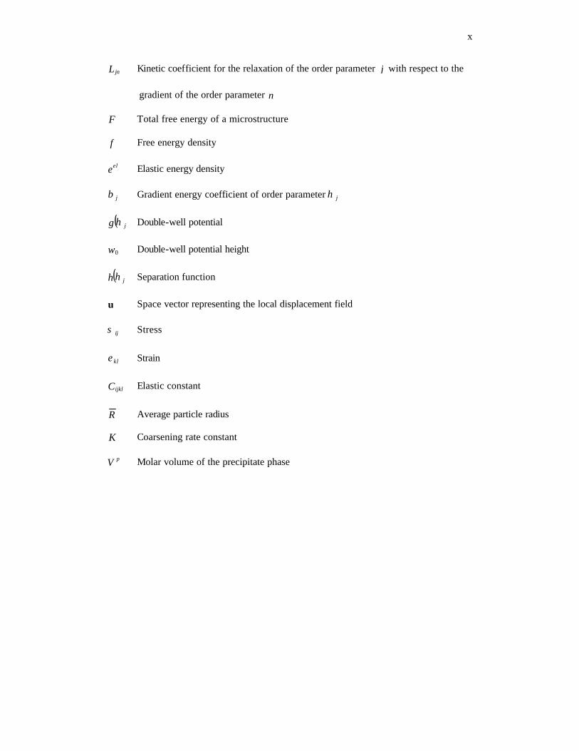
x
jnL Kinetic coefficient for the relaxation of the order parameter j with respect to the
gradient of the order parameter n
F Total free energy of a microstructure
f Free energy density
ele Elastic energy density
jβ Gradient energy coefficient of order parameter jη
( )jg η Double-well potential
0w Double-well potential height
( )jh η Separation function
u Space vector representing the local displacement field
ijσ Stress
klε Strain
ijklC Elastic constant
R Average particle radius
K Coarsening rate constant
pV Molar volume of the precipitate phase
Page 11
xi
List of Figures
Figure 1.1 An integrated four-stage multi-scale approach for multi-component materials
modeling, simulation and design. 7
Figure 2.1 Calculated linear thermal expansion coefficient of fcc Al in comparison with
experimental data from the literature. 27
Figure 2.2 Comparison of lattice parameter data for Al and the model calculation. The
dotted and solid lines represent the results from Equation 2.8
( [ ])500(1001.1)500(1068.1exp0708.4 2285 −×+−×= −− TTa and
3103.1 −×=NS Å) and Equation 2.9
( [ ]1)500(1001.1)500(1068.10708.4 2285 +−×+−××= −− TTa and
3103.1 −×=NS Å), respectively. 28
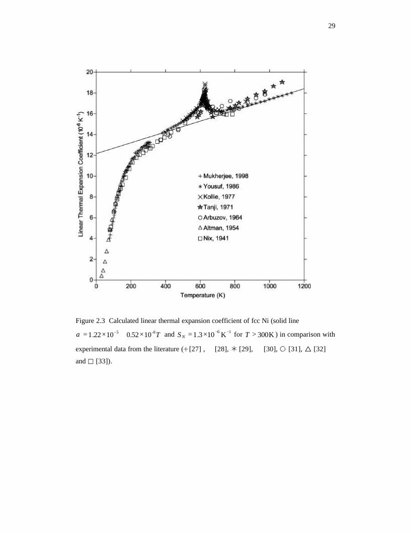
Figure 2.3 Calculated linear thermal expansion coefficient of fcc Ni (solid line
T-85 1052.01022.1 ×+×= −α and 16 K103.1 −−×=NS for K300>T ) in
comparison with experimental data from the literature. 29
Figure 2.4 Comparison of lattice parameter data for Ni and the model calculation (solid
line [ ]1)900(1026.0)900(1022.15560.3 2285 +−×+−××= −− TTa and
3106.3 −×=NS Å). 30
Figure 2.5 Order parameter vs. temperature curve for the Ni-25at% Al alloy. 31
Figure 2.6 Average composition in the γ phase as a function of the holding time during
measurement at 953K. The initial and final compositions (dotted lines) refer to
Page 12
xii
the equilibrium compositions at the previous annealing temperature (973K)
and the measurement temperature (953K), respectively. 32
Figure 2.7 Room-temperature lattice parameter of the γ phase in the Ni-Al system. The
solid line represents the results of the model calculation ( 3104.6 −×=NS Å).
33
Figure 2.8 Temperature dependence of the lattice parameter of the γ phase in various
Ni-Al alloys. The solid lines represent the results of the model calculation.
34
Figure 2.9 Room-temperature lattice parameter of the γ ’ phase. The solid line represents
the results of the model calculation ( 3104.7 −×=NS Å). 35
Figure 2.10 Temperature dependence of the γ ’ lattice parameter. The solid lines
represent the results of the model calculation. 36
Figure 2.11 The comparison of the experimental relative thermal expansion of the γ ’
phase (25 at% Al) and the model calculation (solid line) ( %06.0=NS ).
37
Figure 2.12 The calculated misfit between the γ and γ ’ phases. The solid curve shows
the misfit under the equilibrium condition, and the dashed lines represent
those under the frozen composition assumption ( 4101.4 −×=NS ). 38
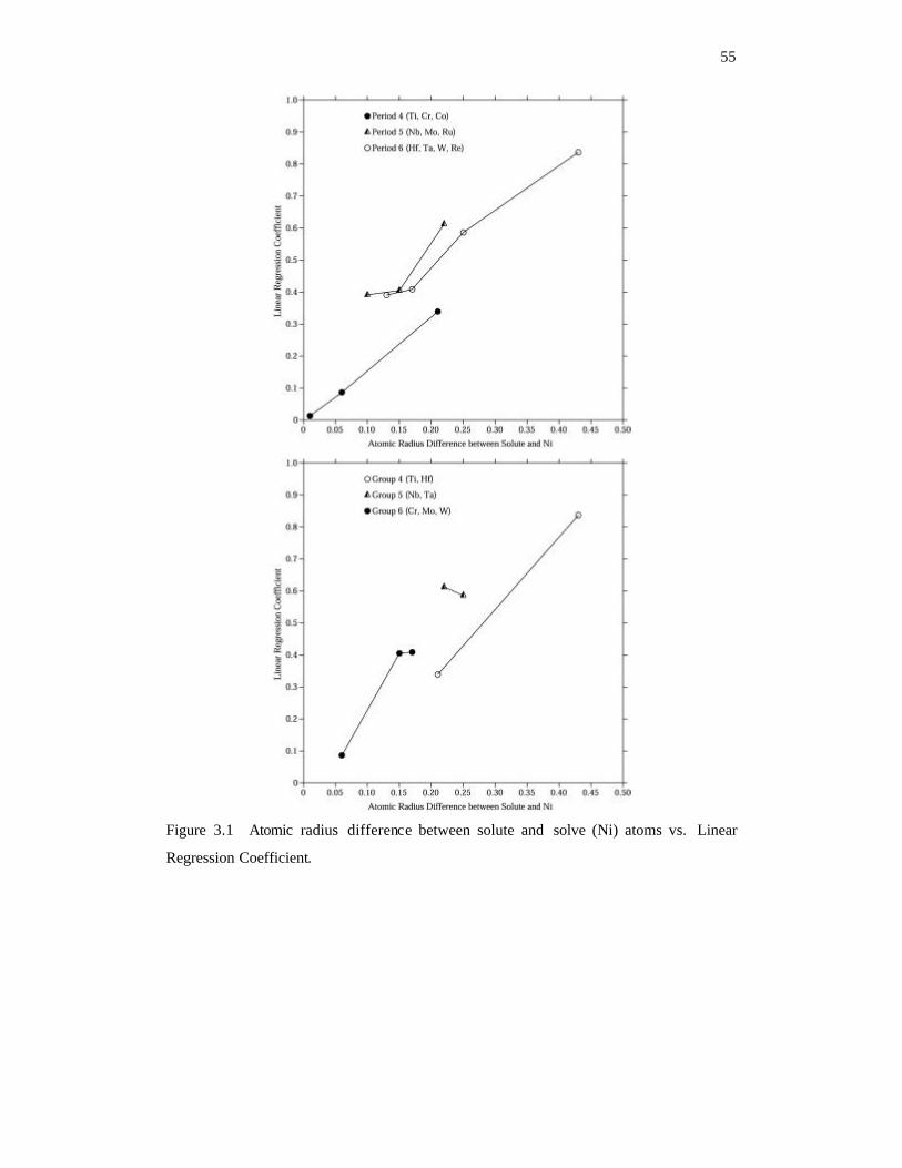
Figure 3.1 Atomic radius difference between solute and solve (Ni) atoms vs. Linear
Regression Coefficient. 55
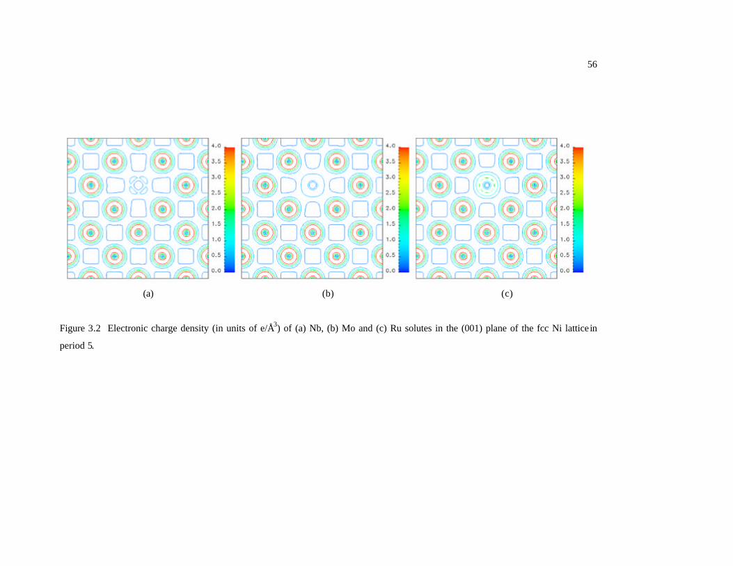
Figure 3.2 Electronic charge density (in units of e/Å3) of (a) Nb, (b) Mo and (c) Ru
solutes in the (001) plane of the fcc Ni lattice in period 5. 56
Page 13
xiii
Figure 3.3 Electronic charge density (in units of e/Å3) of (a) Nb and (b) Ta solutes in the
(001) plane of the fcc Ni lattice in group 5. 57
Figure 3.4 Lattice parameter changes in Ni (γ ) solid solutions with additions of Al and
W ( 0059.0=NS Å for Al and 0015.0=NS Å for W). 58
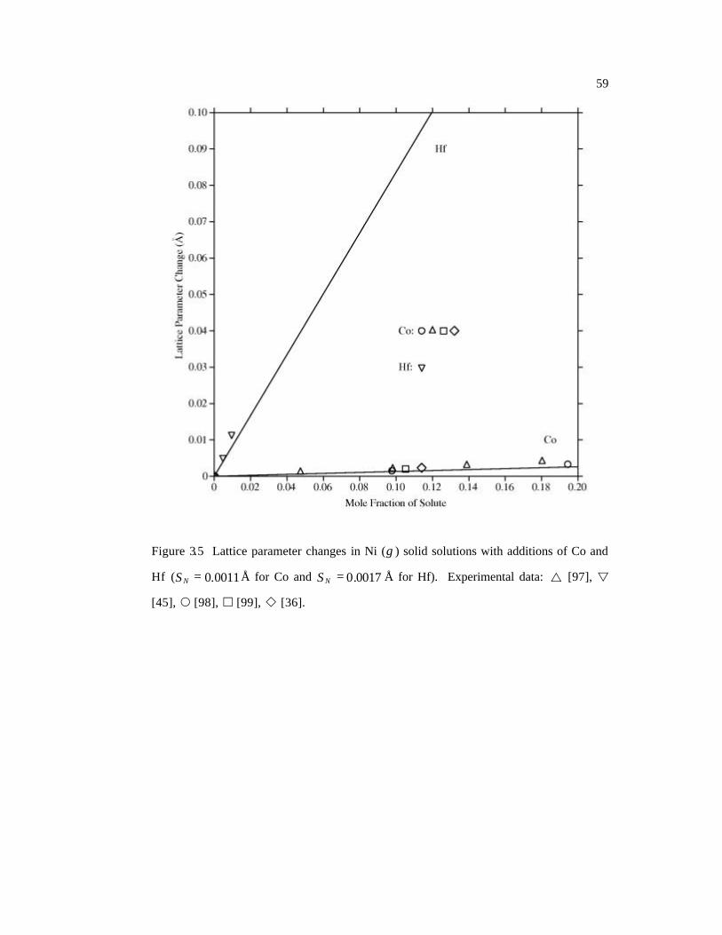
Figure 3.5 Lattice parameter changes in Ni (γ ) solid solutions with additions of Co and
Hf ( 0011.0=NS Å for Co and 0017.0=NS Å for Hf). 59
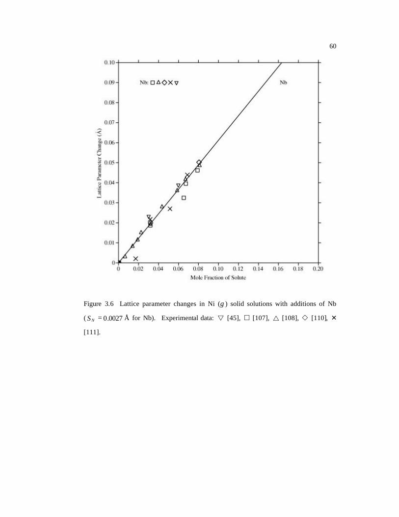
Figure 3.6 Lattice parameter changes in Ni (γ ) solid solutions with additions of Nb
( 0027.0=NS Å for Nb). 60
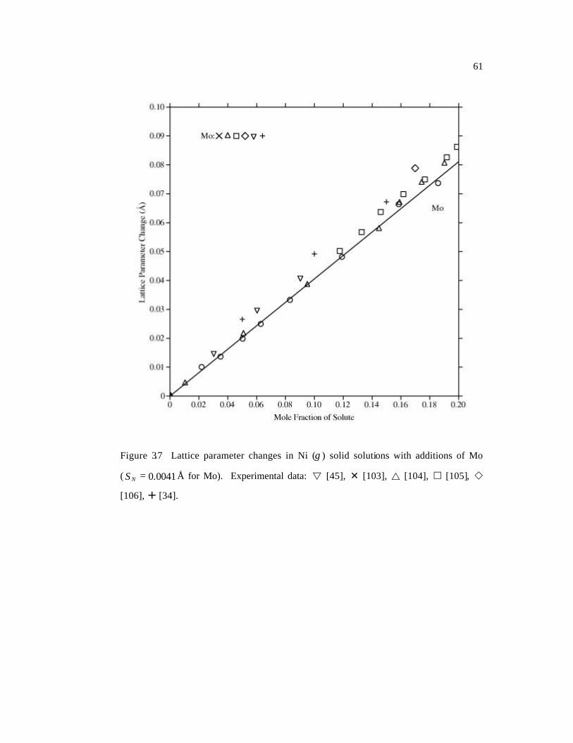
Figure 3.7 Lattice parameter changes in Ni (γ ) solid solutions with additions of Mo
( 0041.0=NS Å for Mo). 61
Figure 3.8 Lattice parameter changes in Ni (γ ) solid solutions with additions of Re and
Ta ( 0013.0=NS Å for Re and 0026.0=NS Å for Ta). 62
Figure 3.9 Lattice parameter changes in Ni (γ ) solid solutions with additions of Ru
( 0055.0=NS Å for Ru). 63
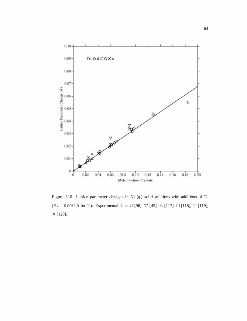
Figure 3.10 Lattice parameter changes in Ni (γ ) solid solutions with additions of Ti
( 0011.0=NS Å for Ti). 64
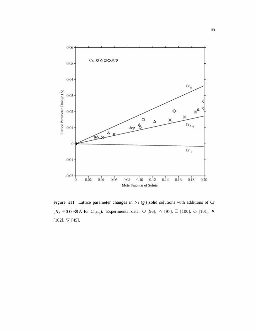
Figure 3.11 Lattice parameter changes in Ni (γ ) solid solutions with additions of Cr
( 0088.0=NS Å for CrAvg). 65
Page 14
xiv
Figure 4.1 Lattice misfit between γ and γ ’ in the Ni-Al binary system. Curves present
calculated results, and symbols are reported experimental values from
literature. 76
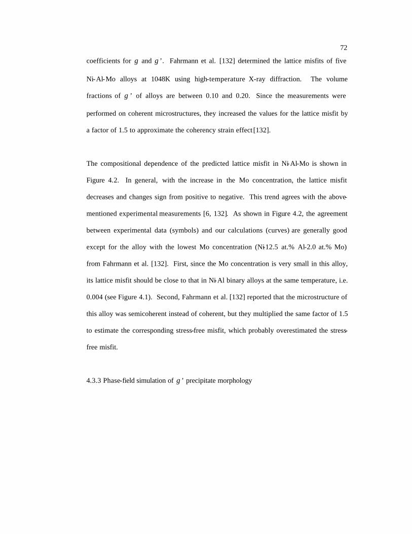
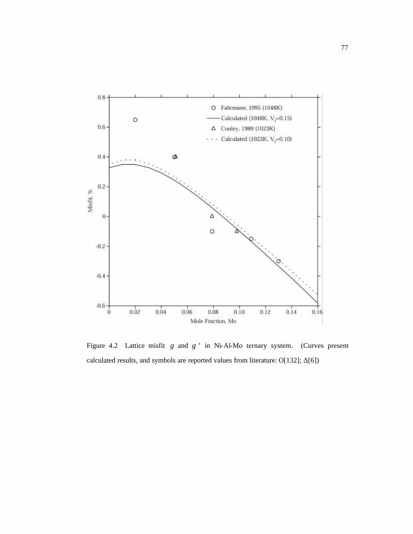
Figure 4.2 Lattice misfit γ and γ ’ in Ni-Al-Mo ternary system. Curves present
calculated results, and symbols are reported values from literature. 77
Figure 4.3 Comparison of precipitate morphologies, obtained by experiments. (a) and
2D phase-field simulations (b, c) in a Ni-12.5 at.% Al-2.0 at.% Mo alloy aged
at 1048K for 67h: (b) 0065.0=δ ; (c) 0035.0=δ . 78
Figure 5.1 Chemical diffusivity in the γ phase for Ni-Al as a function of Al
composition. The symbols are experimental data, and the solid line are
calculated from the mobility database developed by Engstrom and Agren.
98
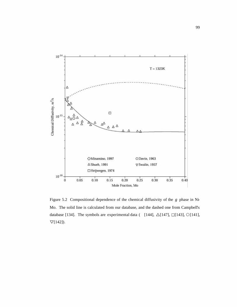
Figure 5.2 Compositional dependence of the chemical diffusivity of the γ phase in Ni-
Mo. The solid line is calculated from our database, and the dashed one from
Campbell’s database. The symbols are experimental data. 99
Figure 5.3 Chemical diffusivities of the γ phase in Ni-15 at%Mo and Ni-3 at%Mo as a
function of inverse temperature. The solid lines are calculated from our
database, and the dashed ones from Campbell’s database. The symbols are
experimental data. 100
Figure 5.4 Diffusion coefficient of Mo in Al as a function of inverse temperature. The
solid line is calculated from our database, and the dashed one from
Campbell’s database. The symbols are experimental data. 101
Page 15
xv
Figure 5.5 Tracer diffusivities of Ni in the stoichiometric Ni3Al. The solid line is
calculated from the assessment I, and the symbols present experimental data.
102
Figure 5.6 Chemical diffusivities in the stoichiometric Ni3Al. The solid line is calculated
from the assessment I, and the symbols present experimental data. 103
Figure 5.7 Calculated chemical diffusivity (assessment I) compared with the
experimental data from Fujiwara and Horita. 104
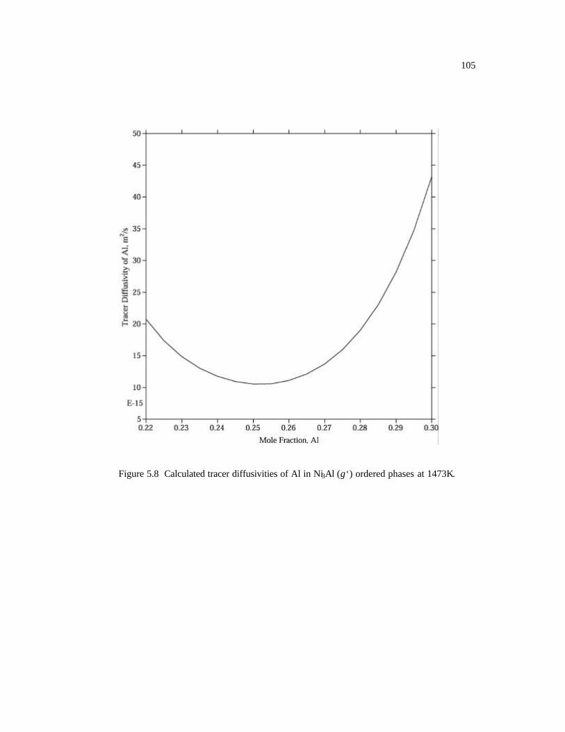
Figure 5.8 Calculated tracer diffusivities of Al in Ni3Al (L12) ordered phases at 1473K.
105
Figure 5.9 Concentration of the anti-site Al in Ni3Al (L12) ordered phases at 1473K.
106
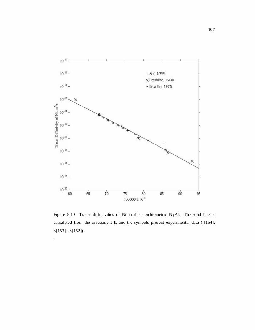
Figure 5.10 Tracer diffusivities of Ni in the stoichiometric Ni3Al. The solid line is
calculated from the assessment II, and the symbols present experimental data.
107
Figure 5.11 Chemical diffusivities in the stoichiometric Ni3Al. The solid line is
calculated from the assessment II, and the symbols present experimental data.
108
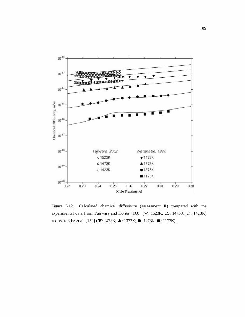
Figure 5.12 Calculated chemical diffusivity (assessment II) compared with the
experimental data from Fujiwara and Horita. 109
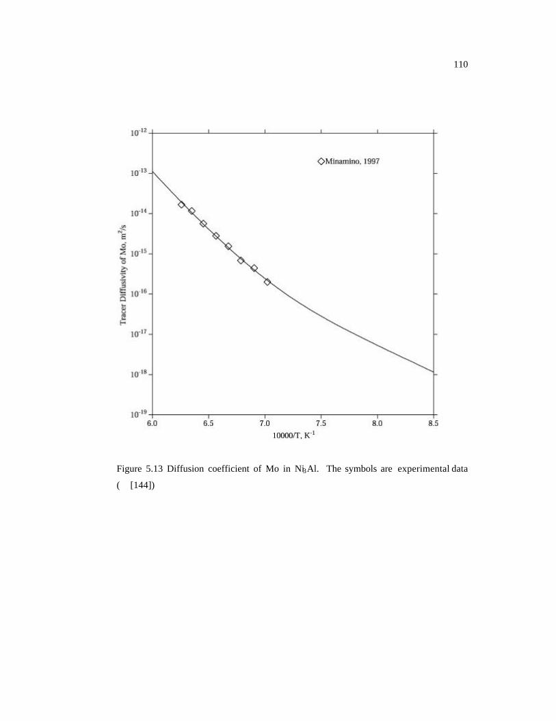
Figure 5.13 Diffusion coefficient of Mo in Ni3Al. The symbols are experimental data.
110
Page 16
xvi
Figure 6.1 Isothermal section of Ni-Al-Mo ternary phase diagram at 1048K. Symbols
show the compositions of selected samples and dotted lines present the tie-
lines for those compositions. 124
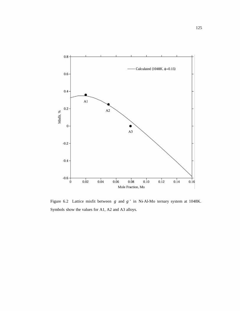
Figure 6.2 Lattice misfit between γ and γ ’ in Ni-Al-Mo ternary system at 1048K.
Symbols show the values for A1, A2 and A3 alloys. 125
Figure 6.3 Microstructure evolution of the γ ’ precipitates in Ni-Al-Mo alloys at 1048K.
Figures in the bottom row are from experiments, and others from 2D phase-
field simulations. 126
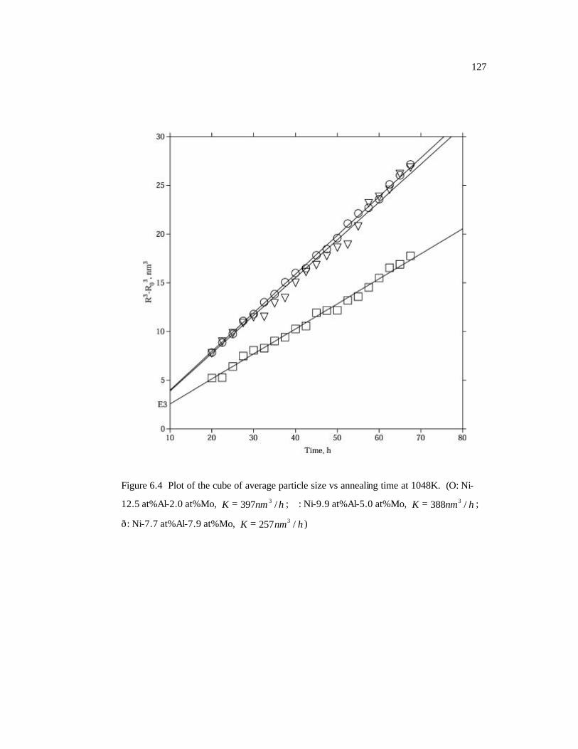
Figure 6.4 Plot of the cube of average particle size vs annealing time at 1048K. 127
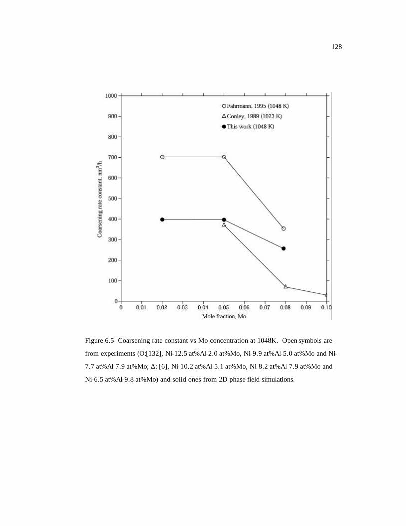
Figure 6.5 Coarsening rate constant vs Mo concentration at 1048K. Open symbols are
from experiments and solid ones from 2D phase-field simulations. 128
Figure 6.6 Comparison of various ( )φf functions from different theories. 129
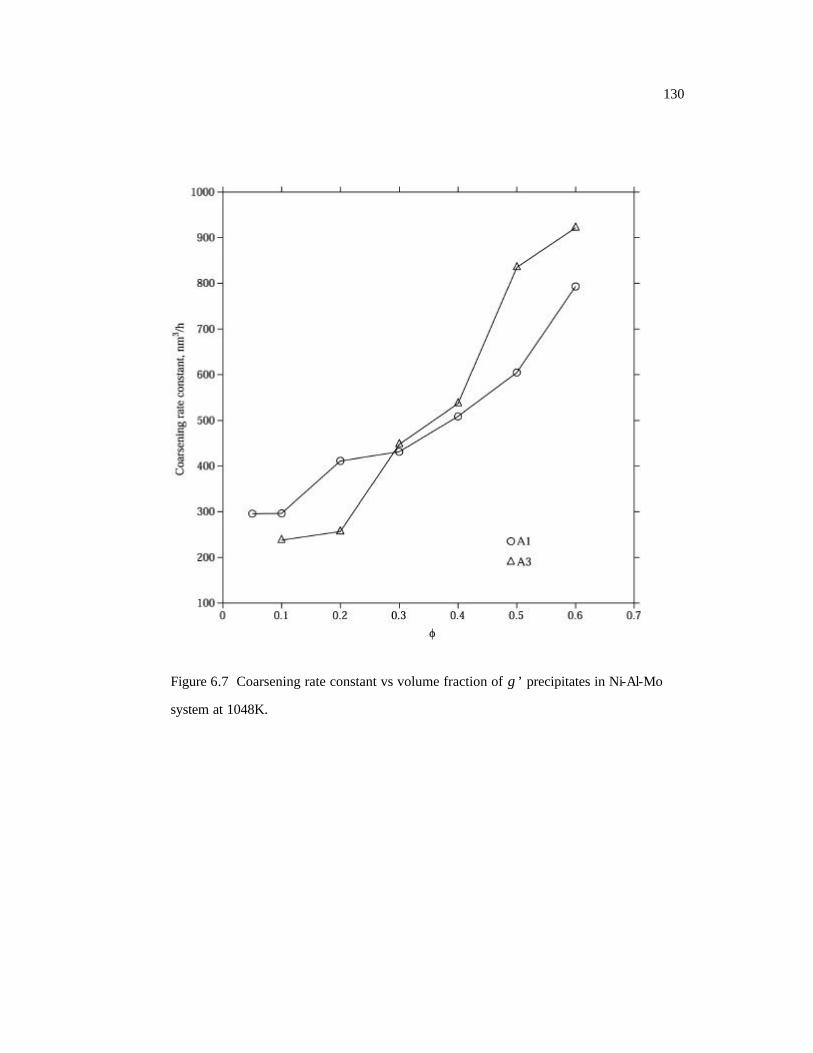
Figure 6.7 Coarsening rate constant vs volume fraction of γ ’ precipitates in Ni-Al-Mo
system at 1048K. 130
Figure C.1 Interactions between Al and Ni in the same sublattice. The open symbols are
calculated with constrained relaxations and the solid ones are from
unconstrained relaxations. 151
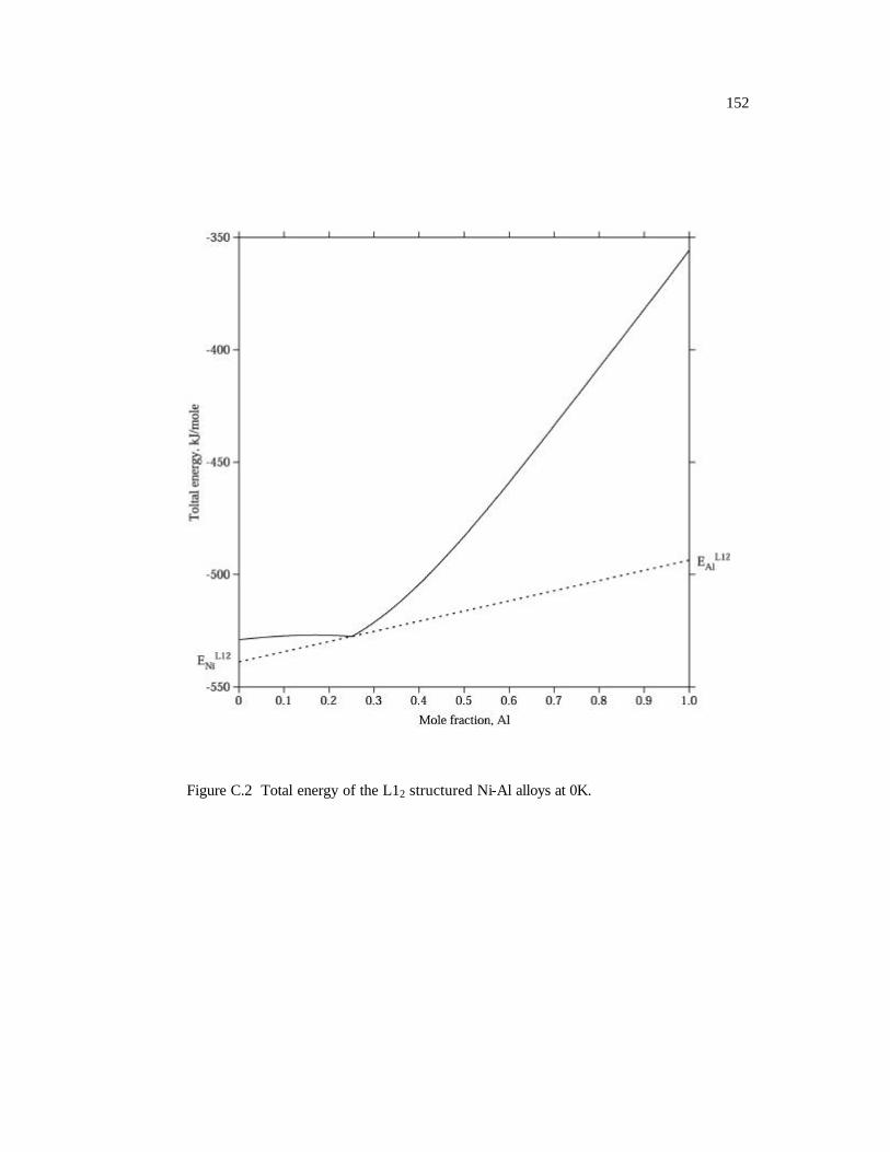
Figure C.2 Total energy of the L12 structured Ni-Al alloys at 0K. 152
Page 17
xvii
List of Tables
Table 2.1 The optimized parameters for the γ and γ ’ phases in Ni-Al system (in Å).
26
Table 3.1 Total energies and lattice parameters for Ni107X1 fcc solutions from first-
principles calculations. 50
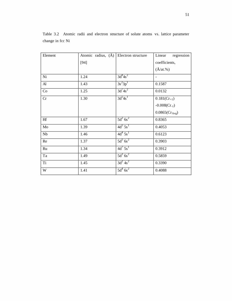
Table 3.2 Atomic radii and electron structure of solute atoms vs. lattice parameter
change in fcc Ni. 51
Table 3.3 Local lattice distortion in fcc Ni (in pm). 52
Table 3.4 Linear regression coefficients of solute atoms in fcc Ni (in Å/at.%). 53
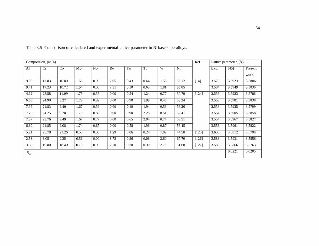
Table 3.5 Comparison of calculated and experimental lattice parameter in Ni-base
superalloys. 54
Table 4.1 Lattice parameters of ordered and disordered phases. 75
Table 4.2 Linear coefficients of solute or anti-site elements in the γ and γ ’ phases (in
Å/at.%). 75
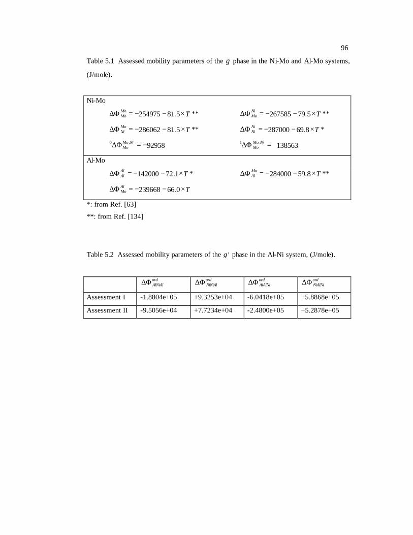
Table 5.1 Assessed mobility parameters of the disordered fcc phase in the Ni-Mo and Al-
Mo systems, (J/mole). 96
Table 5.2 Assessed mobility parameters of the ordered L12 phase in the Al-Ni system,
(J/mole). 96
Table 5.3 Formation energy of vacancy in the Ni3Al ordered phase. 97
Table 5.4 Model parameters for chemical ordering of L12 in Ni-Al-Mo, (J/mole). 97
Table 6.1 Some parameters for phase-field simulations ( KT 1048= ). 123
Page 18
xviii
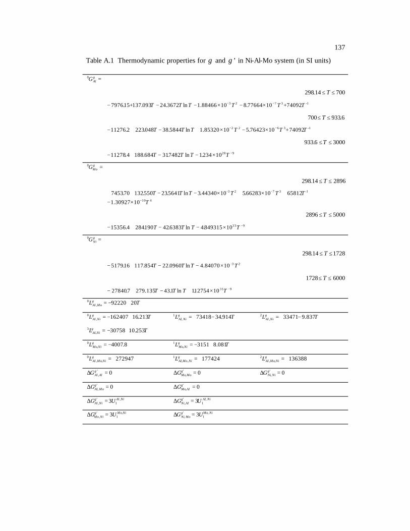
Table A.1 Thermodynamic properties for γ and γ ’ in Ni-Al-Mo system (in SI units)
137
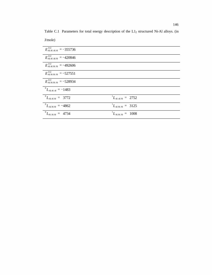
Table C.1 Parameters for total energy description of the L12 structured Ni-Al alloys. (in
J/mole) 146
Table C.2 Structural descriptions of the SQS structure for L12 alloys. A and B are
randomly distributed species in one sublattice and C and D are atoms
occupying the other three sublattices. The atomic positions are given in direct
coordinates, and are for the ideal, unrelaxed structures. 147
Page 19
xix
ACKNOWLEDGEMENTS
I wish to express my sincere gratitude to my advisors, Dr. Zi-Kui Liu and Dr. Long-Qing
Chen, for their constant advice, guidance and encouragement during my four-year Ph.D.
study at the Pennsylvania State University (PSU). I also wish to thank Dr. Jorge O. Sofo,
Dr. Padma Raghavan for their help and encouragement, and serving in my thesis
committee.
The assistance from Dr. Chris Wolverton of Ford Research Laboratory and Dr. Qiang Du
of the Department of Mathematics in my thesis research is gratefully acknowledged. I
also want to thank Dr. Michael G. Fahrmann of Special Metals Corp for providing the
original TEM micrographs.
I would also take the opportunity to thank all members in Dr. Zi-Kui Liu and Dr. Long-
Qing Chen’s research groups, as well as the faculty and staff of the Department of
Materials Science and Engineering, for their help and cooperation during my stay at PSU.
Finally, I would like to thank my parents, for their constant encouragement and
invaluable support without which this thesis could not have come true.
Page 20
1
Chapter 1
Introduction
Since the microstructure (the size, shape, and spatial arrangement of the structural
features) plays a critical role in determining various properties of a material, e.g.
mechanical, electrical, magnetic and optical properties, the study of microstructures is a
very important portion in the field of materials science and engineering, and
microstructure controlling is vital process to obtain a material of desired properties. Used
in aircraft engines, Ni-base superalloys are demanded to be thermodynamically and
structurally stable at high temperatures and for a long period of time due to the high-
temperature operating environment of the aircraft engines. The microstructure of Ni-base
superalloys consists of γ ’ precipitates and a face-centered cubic (fcc) matrix γ . γ ’ has
an ordered fcc structure (L12) where one type of atoms prefer the face-centered sites and
the corner positions are occupied by another type of atoms. In Ni-base superalloys, the
γ ’ precipitate coherently embedded in the γ matrix is the primary strengthening phase,
and its volume fraction, morphology and size distribution strongly affects the mechanical
properties of the materials (e.g. strength, fatigue and creep). Thus the control of the
γ + γ ’ two-phase microstructure and its high-temperature stability becomes the key for
designing of Ni-base superalloys.
Page 21
2
As a result of those fine γ ’ particles, a large surface area is presented, and thus the total
free energy can be decreased by smaller particles dissolving and mass transporting from
those smaller particles to larger ones. Such a process is called Ostwald ripening or
coarsening, which occurs at later stages of phase transformations. Due to the high service
temperature of Ni-base superalloys, coarsening is an important issue during service.
Thus a knowledge of the coarsening process of the γ ’ precipitates is essential for design
and application of Ni-base superalloys.
Since there are many factors, e.g. lattice misfit between the precipitate and matrix,
coherency of interface and diffusivities of various elements, affecting the microstructure
evolution and coarsening process, the theoretical predictions with the aid of computer is
the only practicable way for a systematic investigation on a complex system.
In current laboratory and industrial practice, the traditional trial-and-error method is still
a dominant technique to optimizing the alloy chemistry and processing conditions for
achieving desirable microstructures and mechanical properties of Ni-based superalloys.
This often highly expensive and empirical approach becomes more and more insufficient
to meet today’s increasingly demanding applications, and has been complemented by
various computational tools in last few decades. Due to the advances in computer and
information technology, computational materials science has been quickly developed,
and the required experiments can be dramatically reduced with the help of it. Some very
useful computational tools for materials scientists are atomic-scale first-principles
Page 22
3
approach, CALPHAD (CALculation of PHAse Diagram) technique and phase-field
simulation.
Based on the density functional theory (DFT) [1], the first-principles approach can
calculate thermodynamic properties (e.g. enthalpy and entropy of formation), kinetic data
(e.g. diffusivity) and crystallography information (e.g. lattice parameter and interfacial
energy) using only the atomic numbers and crystal structure information as the inputs.
By considering the configurational and vibrational contributions, various properties at
finite temperatures can also be predicted. Although the first-principles approach has been
improved and extensively used in many fields in recent years, it is still unpractical to
determine the total energy for multi-component systems directly from the first-principles
approach, at least the accuracy is not comparable to the experimental measurements.
Another important tool in computational materials science, the CALPHAD approach [2]
is very powerful in predicting phase equilibria and phase transformations of multi-
component alloys. The CALPHAD approach allows one to determine the
thermodynamic descriptions for various phases in the multi-component system, and then
constructs the thermodynamic database. Both experiments and first-principles
calculations on simple low-order systems can provide data for deriving model parameters,
and various thermodynamic properties can be calculated from the thermodynamic
database. A similar strategy can be adopted for developing kinetic databases and
databases for lattice parameters, elastic constants and interfacial energies as a function of
composition and temperature [3].
Page 23
4
The phase-field approach is one of the most powerful methods for modeling various
microstructure-related processes [4]. It describes a microstructure by a set of conserved
or non-conserved field variables, and those variables change smoothly from one
phase/domain to another across the interfacial region. Unlike other microstructure
models, the phase-field approach does not explicitly track the positions of interfaces, and
hence the temporal evolution of arbitrary microstructure can be predicted without any a
priori assumptions about their evolution path [3].
Recently, Liu and co-workers proposed a prototype to integrate various computational
tools for multi-component materials simulation and design [3]. The framework is shown
in Figure 1.1, and involves four major computational steps:
• Atomic-scale first-principles calculations for predicting thermodynamic properties,
kinetic data and crystallography information;
• CALPHAD (CALculation of PHAse Diagram) approach for developing
thermodynamic, kinetic and crystallographic databases;
• Phase-field modeling for simulating the evolution of microstructures;
• Finite element analysis for deriving mechanical properties from the simulated
microstructures.
As part of the framework, the present thesis is concerned with the first three steps, from
first-principles calculations to phase-field simulations. The main goal of this
investigation is to predict the microstructure evolution and coarsening kinetics of γ ’
precipitates in Ni-base superalloys by integrating these computational tools. As one of
Page 24
5
the commonly used alloy elements in Ni-base superalloys, Mo can not only adjust the
lattice misfit between γ and γ ’ [5], but also control the coarsening rate of γ ’
precipitates [6]. Therefore, we focus our current study on Ni-Al-Mo superalloys.
Three objectives are planned for this work. The first objective is to develop a lattice
parameter database for the γ and γ ’ phases in the Ni-base superalloys, and then the
lattice misfit can be calculated from the database and employed to phase-field simulations.
In Chapter 2, we propose a phenomenological model to describe the lattice parameters of
substitutional solid solution as a function of temperature and composition. It is applied to
the γ and γ ’ phases in Ni-Al binary alloys and the model parameters are evaluated using
the CALPHAD approach from available experimental data in the literature. Since the
experimental results are usually very limited in multi-component systems, an integrated
computational approach is then developed in Chapter 3 for evaluating the lattice misfit
between γ and γ ’ in Ni-base superalloys by combining first-principles calculations,
existing experimental data and phenomenological modeling. In particular, the lattice
misfits in Ni-Al and Ni-Al-Mo alloys are studied by this approach. With the help of first-
principles calculations, we also study the effects of various alloy elements on the lattice
parameter and the local lattice distortion around the solute atom in binary fcc-Ni
solutions, which is shown in Chapter 4. The solute atoms considered include Al, Co, Cr,
Hf, Mo, Nb, Re, Ru, Ta, Ti and W. The contribution from the atomic size difference, the
electronic interactions, and the magnetic spin relations are discussed. Based on the
results from first-principles calculations, the linear composition coefficients of fcc Ni
Page 25
6
lattice parameter for different solutes are determined, and the lattice parameters of multi-
component Ni-base superalloys as a function of solute composition are predicted.
The second objective is to construct an atomic mobility database for Ni-Al-Mo
superalloys. In particular, diffusion in disordered γ and ordered γ ’ phases is modeled in
Chapter 5 using phenomenological models provided by Andersson and Agren [7] and
Helander and Agren [8]. Diffusion data in various constituent binary systems are
collected from the literature and assessed to establish the kinetic database, and previous
modeling works for γ are reviewed and revised. The diffusion mechanisms in the
ordered γ ’ phase are discussed based on the results, and used to refine atomic mobility
modeling.
Finally, for the third objective, the mic rostructure evolutions and coarsening kinetics of
γ ’ precipitates in Ni-Al-Mo ternary alloys will be predicted by phase-field simulations in
Chapter 6. All simulations are linked with thermodynamic, kinetic and lattice parameter
databases to provide predictions in terms of experimental time and length scales. Both
the effects from volume fraction of precipitates and compositions are studied.
Page 26
7
Figure 1.1 An integrated four-stage multi-scale approach for multi-component materials
modeling, simulation and design. Redrawn from [3]
First-principles calculations and experiments
Thermodynamic data of unary binary and ternary systems
Kinetic data of unary, binary and ternary systems
Interfacial energies, lattice parameters, elastic constants
CALPHAD approach to data optimization
Thermodynamic database for multi-component systems
Kinetic database for multi-component systems
Databases for lattice parameters, elastic constants, and interfacial energies
A multi-component phase-field model
Elastic constants and plasticity of phases
Simulated microstructures in 2 and 3 dimensions
OOF: Object-oriented finite element analysis of material microstructure
Mechanical response of simulated microstructures
Page 27
8
Chapter 2
Modeling of Lattice Parameter
2.1 Background
The lattice parameter and thermal expansion are two important material properties that
are strongly correlated to many thermophysical properties. Because of their importance
in both theoretical study and practical applications, a large number of studies have been
carried out on this subject from many different points of view, using theoretical,
experimental, and empirical approaches. The composition dependency of lattice
parameters was modeled in various ways, such as elasticity theory, various potential
approaches, and first-principle calculation, but none of them is very successful [9],
neither simple nor accurate enough. The most widely used prediction of the lattice
parameters across a solid solution was the linear relationship proposed by Vegard [10].
However, the investigations on metallic systems always show some deviations from
Vegard’s law, because Vergard’s law is only valid when the electronic environment of
both atoms is undisturbed by the formation of the solid solution, but in reality electrons in
states just below the Fermi level can also participate in metallic bonding [11]. Due to the
limited and scattered experimental data, the temperature effect on the lattice parameter is
often overlooked, especially for multi-component alloys. In many cases, such an effect is
assumed to be small enough to be neglected or approximated by some arbitrary
polynomials (the linear relationship is often suggested). However, such an assumption is
Page 28
9
seldom supported by the experimental results except in a very narrow temperature region.
In this chapter, a simple phenomenological model is developed to describe the lattice
parameters of solid solution phases as a function of composition and temperature. In
Section 2.2, the temperature effect on the linear expansion coefficient ( Lα ) of the pure
element is considered first, and the lattice parameters of pure elements are then calculated
from the thermal expansion. The contribution from substitutional solute is treated using
an approach similar to that used in the Gibbs energy modeling [12]. At the end of the
Section 2.2, the modeling of chemical ordering effect is discussed in relation to the
sublattice model. In Section 2.3, this model is applied to the Ni-Al system, the most
important constituent binary system in Ni-based superalloys, to calculate the difference
between the lattice parameters of precipitate γ ’ (L12) and matrix γ (fcc_A1), which
plays a very important role in the microstructure evolution and properties of Ni-based
superalloys [13-16]. We evaluate the model parameters describing the lattice parameters
of the γ ’ and γ phases, and then calculate the lattice misfit between these phases.
2.2 Models
2.2.1 Pure Element
Based on quantum physics, Ruffa [17] proposed the following equation to describe the
thermal expansion coefficients
Page 29
10
)(2
33
DDn
L xgT
Dwrk
=
θα (2.1)
where T is the temperature, k is Boltzmann’s constant, w and D are the inverse width
and depth, respectively, of the Morse potential, nr the nearest neighbor distance, Dθ the
Debye temperature, and Tx DD /θ= . The integral )( Dxg is given by
∫ −=
Dx
x
x
D dxe
exxg
0 2
4
)1()( (2.2)
Since the Equation 2.1 only considers the first order in the frequency, it is usually
accurate only up to about Dθ7.0 , but gives the dominant contribution over the entire
temperature range. To extend this formula to higher temperatures, a correction term was
added [17].
+
= )(
2)(
23
1
3
DDDn
L xgD
kTxg
TDwr
kθ
α (2.3)
where
∫ −+
=Dx
x
xx
D dxe
eexxg
0 3
5
1)1(
)1()( (2.4)
For low temperatures ( DT θ<< ), one can obtain
34
52
≈
DnL
TDwr
kθ
πα (2.5)
which implies Lα is proportional to the 3T for DT θ<< . When the temperature is high
( DT θ>> ),
Page 30
11
+++
+≈TD
kT
Dk
Dk
Dwrk DDD
nL
110438
331
23 2θθθ
α (2.6)
Because the contribution of the T/1 term is not significant at high temperatures, Lα vary
almost linearly with temperature in the high temperature range, which will be adopted in
the present work, i.e., we can describe the thermal expansion coefficient by a linear
function of temperature as a first approximation.
BTAL +=α (2.7)
The parameters A and B can be defined by available information from the thermal
expansion experiments. Such a linear relationship was observed by several investigations
[18-20].
The lattice parameters a can be obtained from Equation 2.7 through integration of Lα
based on the definition dTda
aL
1=α , and the lattice parameter ( 0a ) at a given temperature
( 0T ) can be used to determine the integration constant
−+−= )(
2)(exp 2
02
00 TTB
TTAaa (2.8)
Lα is about 510− K-1 for metals, so the relative change in lattice parameter is very small
(about 1% with a change of 1000K in temperature), thus the lattice parameter can be
approximated by the following polynomial
+−+−= 1)(
2)( 2
02
00 TTB
TTAaa (2.9)
In the Section 2.3, we calculate the lattice parameters of Al by both Equations 2.8 and 2.9,
and the results are almost identical.
Page 31
12
2.2.2 Binary System
Similar to the Gibbs energy modeling [12], we add an excess contribution to describe the
deviation of the lattice parameter from the Vegard’s law. Such a phenomenological model
can be written as
aaxa ex
iii += ∑ 0 (2.10)
where ix is the mole fraction of element i . ia0 denotes the lattice parameter of pure
element i defined by Equation 2.9. aex is the excess contribution expressed in the
Redlich-Kister polynomials [21]
∑∑ ∑> =
−=i ij
n
k
kjiji
kji
ex xxIxxa0
, )( (2.11)
The interaction parameter, jik I , , can be expressed as a function of temperature:
TBAI jik
jik
jik
,,, += (2.12)
2.2.3 Ordered Phase
The ordered phase and related disordered phase can be modeled by the sublattice model
[22, 23]. For a two-sublattice model qp BABA ),(),( , the lattice parameter a can be
expressed by the following equation:
∑∑∑∑∑∑ ∑
∑∑ ∑∑∑
> >>
>
++
+=
i ij k kllkji
IIl
IIk
Ij
Ii
i ij kjik
Ik
IIj
IIi
i ij kkji
IIk
Ij
Ii
i jji
IIj
Ii
IyyyyIyyy
Iyyyayya
,:,,:
:,:0
(2.13)
Page 32
13
where Iiy and II
iy are the site fractions of i in the first and second sublattices. Similar to
Equation 2.12, the interaction parameters kjiI :, , jikI ,: and lkjiI ,:, can be expressed as
functions of temperature. jia :0 , the lattice parameter of the end member qp ji of the
sublattice model, can be written as:
≠+++
++
==
ijTDCaqp
qa
qpp
ijaa
jijiji
i
ji::
00
0
:0 (2.14)
where jiC : and jiD : are model parameters. The overall composition ix is connected with
the site fractions by IIi
Iii y
qpqy
qppx
++
+= . When II
iIii yyx == , the phase is
disordered, and Equation 2.13 is equivalent to Equation 2.10.
2.3 Application to Ni-Al System
In this section we will apply the above phenomenological model to describe the lattice
parameters of γ ’ and γ phases in the Ni-Al system.
2.3.1 Pure Al and Ni
Many reports on the measurement of thermal expansion coefficients and lattice
parameters for Al can be found in the literature. Touloukian et al. [24] referenced 71 sets
of data for Al in their review, and later, Wang and Reeber [25] cited 7 more in their report.
Their selection of experimental data are shown in Figure 2.1. Because the model is not
Page 33
14
applicable to the low temperature range, only the experimental data measured above
300K are used to evaluate the parameters A and B in Equation 2.7. The results are
plotted as the solid line in Figure 2.1.
As shown in Figure 2.1, the coefficient of linear thermal expansion for Al shows a good
linear relationship with temperature from 300 to 800K (standard deviation
17 K107 −−×=NS , calculated as the square root of the sample variance of a set of values
[26]). The low temperature behavior deviates from the linearity because the model only
accurately describes the intermediate temperature behavior. When the temperature is
very high (close to the melting temperature mT ), the experimental results show a visible
deviation from the linear dependence, which is caused by the contribution from thermal
vacancies [25]. Based on the model parameters obtained from the above evaluation, the
lattice parameter of Al can be calculated by Equations 2.8 or 2.9. Figure 2.2 shows the
calculated lattice parameters compared with the experimental data, and it can be seen that
most experimental data can be well reproduced by the present model ( 3103.1 −×=NS Å).
As shown in Figure 2.2, when the temperature increases from the room temperature to the
melting temperature, the lattice parameter of Al only increases 2%. The dotted and solid
lines represent the results from Equations 2.8 and 2.9, respectively, and the differences
between them are less than 0.015%.
Many experimental studies on the thermal expansion of Ni were performed in a wide
temperature range, and more than 100 investigations before 1975 have been reviewed by
Touloukian et al. [24]. Using the dilatometry technique, Kollie [27] measured the
Page 34
15
thermal expansions in temperature range from 300 to 1000K, while Mukherjee et al. [28]
investigated for low temperatures up to 300K. Yousuf et al. [29] studied the magnetic
effect on the lattice expansion of Ni by high-temperature X-ray diffractometry, and
reported the lattice parameters and the thermal expansion coefficients. The data [27-33]
are plotted in Figure 2.3. The experimental data show a clear peak around the Curie
temperature CT (633K) of Ni, which means the magnetic phase transition has significant
effect on the thermal expansion. In the low temperature range, the experimental results
are in good agreement with each other. However, at the high temperatures, the thermal
expansion coefficient by Yousuf et al. [29] is lower than those in previous reports [30, 31].
Since the purity of their samples [29] is higher than the others, the results from Yousuf et
al. [29] were used to determine the model parameters in Equation 2.7 in the present work.
The calculated linear thermal expansion coefficient of Ni is shown in Figure 2.3 as the
solid line. The low-temperature data ( K300<T ) were not used in the parameter
determination, and deviate from the solid line because Equation 2.7, as discussed in the
previous section, is only applicable in the high temperature range.
Lattice parameters for Ni have been measured by many investigators [29, 34-37]. But the
agreements among their results are quite poor, especially in the high temperature range.
One of the possible reasons is the effect of magnetism that was recently emphasized by
many investigators [28, 29, 38]. Figure 2.4 plots the selected data from the literature.
The poor agreements between the experimental data from different researchers can be
observed in the high temperature range. It therefore seems difficult to define a suitable
mathematic description just on the basis of the experimental lattice parameter data.
Page 35
16
After determining the model parameters in Equation 2.7 from the above experimental
thermal expansion data, the lattice parameter of Ni can be calculated from Equation 2.9.
The calculated lattice parameter is shown in Figure 2.4 by the solid line. In the low
temperature range ( cTT < ), the experimental values are well reproduced by the
calculation ( 3105.1 −×=NS Å). At high temperatures, although the available
experimental data are relatively scattered, our modeling still shows a reasonable
description ( 3101.5 −×=NS Å). As shown in Figures 2.3 and 2.4, changes of slopes of
both thermal expansion and lattice parameter near the Curie temperature were observed
experimentally. To reproduce the phenomena requires a more accurate model that takes
into account the magnetic effect.
In the present work, we chose the 0T in Equations 2.8 and 2.9 as 2/mT , and the 0a is
evaluated from the available experimental data of the lattice parameter.
2.3.2 Binary Ni-Al System
2.3.2.1 Experimental Data
The lattice parameters of the γ solid solution in the Ni-Al system were measured by
several groups [39-45]. Most of those values were measured at room temperature on
samples quenched from high temperatures. The temperature dependence of the lattice
parameter of Ni-Al alloys was investigated by Kamara et al. [40] using high-temperature
Page 36
17
X-ray diffractometry. Another in situ X-ray measurement was performed by Bottiger et
al. [39] on five different composition alloys, and the lattice parameters up to 553K were
reported.
The room-temperature lattice parameters of the 'γ phase were determined by many
investigators [40, 41, 44-59] on samples quenched mostly from 1173-1473K. The
temperature effect on the γ ’ phase were studied by Arbazov and Zelenkov in the
temperature range 293-974K [31] and Taylor and Floyd for 74-1273K [44] by the
dilatometry technique, and their results on the relative thermal expansion agree with each
other. Using high-temperature X-ray diffractometry, Kamara et al. [40], Rao et al. [60]
and Stoeckinger and Neumann [53] investigated the temperature dependencies of the γ ’
lattice parameter. A typical experimental method includes four steps: sample preparation,
heat treatment (homogenization or aging), quench and measurement (mostly at room
temperature). Kamara’s experiment procedure [40] can be described briefly as follows
1) Prepared the Ni-17.7 at% Al alloy by the arc melting;
2) Homogenized the samples at 1273K for 30 minutes and age them at 973K for 168
hours;
3) Quenched the annealed sample to room temperature;
4) Measured the lattice parameters at different temperatures (293, 563, 713, 843,
953K) for 0.6-2 hours.
The measured lattice parameter value is strongly affected by experimental details. On
one hand, the measuring temperature has direct effect on the lattice parameter because of
Page 37
18
the thermal expansion; on the other hand, many experimental conditions can also impact
the lattice parameter by changing the composition and the order parameters of phases.
The order parameter η , the degree of ordering, can be calculated by the site-fraction of
various elements in the ordered phase. For γ ’ in the Ni-Al system, the order parameter
can be defined as
IIAl
IAl
IAl
IIAl
yyyy
+−
=3
η (2.15)
where IAly and II
Aly are the site fractions of Al in the first and second sublattices,
respectively. Using the thermodynamic descriptions by Dupin et al. [61, 62], the change
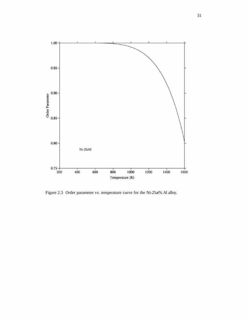
of the order parameter with temperature is shown in Figure 2.5 for the Ni-25 at% Al alloy.
Obviously, the order parameter changes very little in the low temperature range.
During measurement, the compositions of phases change with the measurement
temperature and the measurement time. This evolution can be simulated by Dictra
software [2]. The thermodynamic database from Dupin et al. [61, 62] and the mobility
database from Engstrom and Agren [63] were used in the simulation. Since the
diffusivity in the γ ’ ordered phase is much smaller than that in the γ disordered phase
(about one order of magnitude smaller in Ni-Al system [64]), only the diffusion in the γ
phase was considered in the present simulation. The average simulation size of the γ
phase (~1.5 mµ ) and the measurement temperatures (293, 563, 713, 843, 953K) were
obtained from Kamara’s experiment [40], and the initial composition (12.18 at% Al) is
taken as the equilibrium compositions at the aging temperature (973K). The change of
Page 38
19
the average composition in the γ phase at 953K (the highest measurement temperature in
Kamara’s experiment [40]) is shown in Figure 2.6, and the two dashed lines refer to the
initial composition and the equilibrium composition at 953K, respectively. According to
this figure, the composition will not change significantly during the measurement
(usually less than 3 hours) if the temperature is lower than 953K.
We can thus assume the compositions of the samples measured below the aging
temperature are the same as those at the aging temperature (frozen composition
assumption).
2.3.2.2 Evaluation of Model Parameters
According to Equation 2.10, the lattice parameters of the γ disorder solution can be
described as
)( ,,00 TBAxxaxaxa NiAlNiAlNiAlNiNiAlAl +++= (2.16)
NiAlA , and NiAlB , are model parameters to be evaluated from the experimental data of the
γ phase.
As the γ and γ ’ phases are described with one single Gibbs energy by two sub-lattices
using the formula 13 ),(),( NiAlNiAl [62], for the γ ’ phase, Equation 2.14 is rewritten as
AlAlAl aa 0:
0 = (2.17)
NiNiNi aa 0:
0 = (2.18)
Page 39
20
TDCaaa AlNiAlNiNiAlAlNi ::00
:0 75.025.0 +++= (2.19)
TDCaaa NiAlNiAlNiAlNiAl ::00
:0 25.075.0 +++= (2.20)
Due to the limited experimental data, the following assumptions were made to reduce the
number of independent parameters:
0,:, =NiAlAlNiI (2.21)
TBAI NiAlNiAlNiAl ,:*,:*,:* += (2.22)
)(33 ,:*,:*,:**:, TBAII NiAlNiAlNiAlAlNi +== (2.23)
where the asterisk refers to Al or Ni. Thus, Equation 2.13 can be simplified to
NiAlIINi
IIAlAlNi
INi
IAl
NiNiIINi
INiAlNi
IIAl
INiNiAl
IINi
IAlAlAl
IIAl
IAl
IyyIyy
ayyayyayyayya
,:*,:*
:0
:0
:0
:0
3 ++
+++= (2.24)
Since "' 25.075.0 iii yyx += , and the phase is disordered when "'iii yyx == , we obtain
=++=++
NiAlNiAlAlNiNiAl
NiAlNiAlAlNiNiAl
BDDBACCA
:::,:*
,::,:*
44
(2.25)
Using the experimental lattice parameter values of the γ ’ phase and the previously
obtained parameters NiAlA , and NiAlB , , the parameters of the ordered phase were
evaluated by the parrot module of Thermo-calc software [2]. The compositions and the
site fractions used in the present work were calculated from the thermodynamic
descriptions by Dupin et al. [61, 62]. All available experimental data were selected in the
present evaluation of model parameters, and the data obtained at room temperature were
given very low weight because of the large discrepancies.
Page 40
21
2.3.2.3 Results and Discussion
All model parameters for the lattice parameters of the γ and γ ’ phases in the Ni-Al
system are listed in Table 2.1. It is shown that the lattice parameter of Al has a higher
temperature dependence than that of Ni. The Ni3Al has a rather weak temperature-
dependent lattice parameter, while the hypothetic Al3Ni phase has the highest temperature
dependence. The interaction parameter is negative and becomes more negative with
increasing temperature, which reduces the lattice misfit between γ and γ ’ as discussed
later.
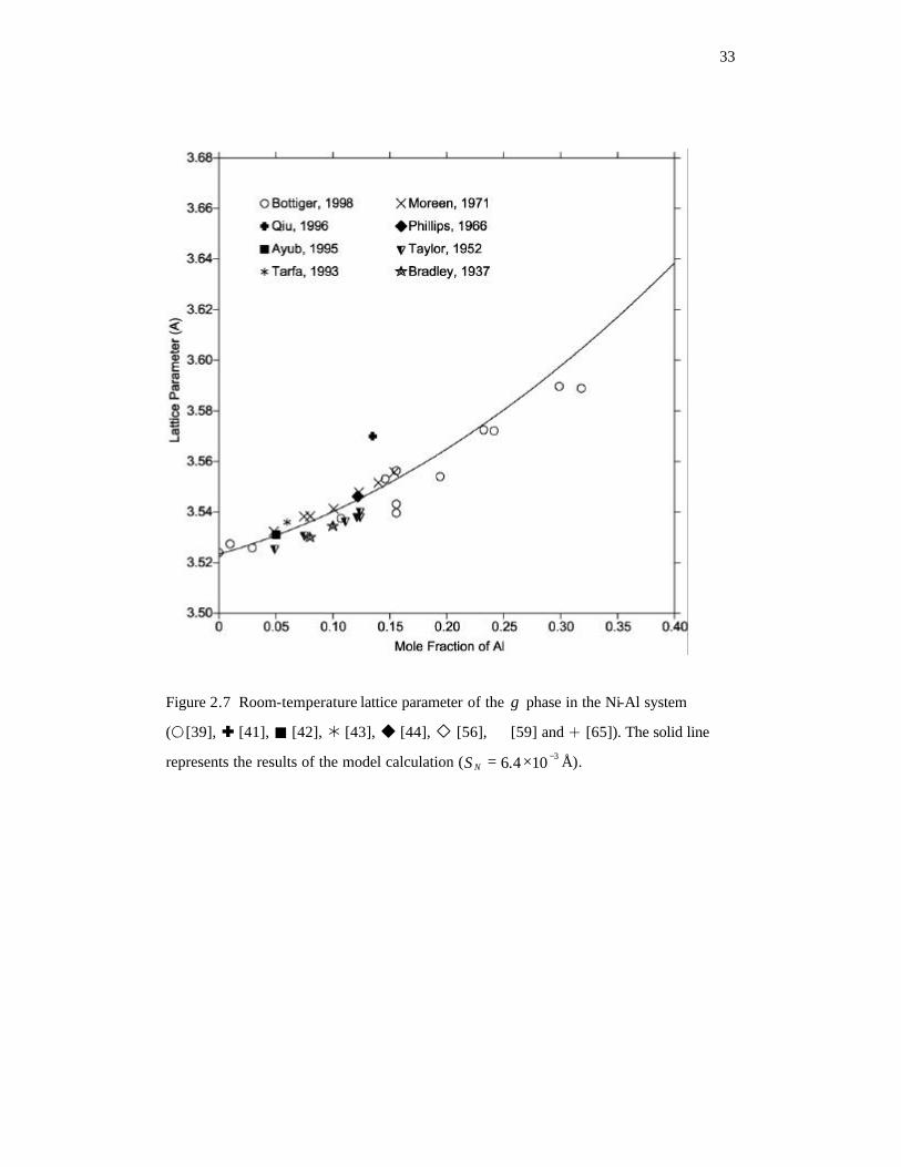
The composition dependence of the lattice parameter of the γ solid solution at room
temperature is calculated and compared with experimental data in Figure 2.7, and the
calculated lattice parameters as a function of temperature for various compositions are
plotted with experimental values in Figure 2.8. Although the trends with temperature are
similar, results by Bottiger et al. [39] are significantly smaller than those reported by
Kamara et al. [40]. It is therefore impossible to reproduce both sets of data. The same
situation appears in the room-temperature data in Figure 2.7, where the values reported
by Bottiger et al. [39] are smaller than other available data [41-43, 65]. Since Bottiger’s
investigation was performed on thin-film samples from sputtering, their results are likely
to be influenced by several processing factors. For example, Bottiger et al. [39] found
that a higher sputtering pressure will reduce the lattice parameter. All experimental data
except for those from Bottiger et al. [39] were selected for the evaluation of model
Page 41
22
parameters, and the calculation can represent most of those experimental data reasonably
well ( 3101.4 −×=NS Å).
The lattice parameters of the γ ’ phase measured at room temperature are plotted in
Figure 2.9, and they are quite scattered. Compared with measurements of the disordered
phase, the lattice parameter of the ordered phase is much more sensitive to experimental
procedures, e.g. heat treatment temperature and time. The treatment history will change
the composition and order parameter, and then cause large discrepancies on the measured
lattice parameters. The composition dependence of lattice parameter of the γ ’ phase at
room temperature was calculated by the present model as the solid line in Figure 2.9, and
the standard deviation NS is 3104.7 −× Å. The calculated curve lies among the
experimental data, and displays a similar slope to those reported by Noguchi et al. [51]
and Aoki and Izumi [52].
The calculated temperature dependence of the γ ’ phase lattice parameter is compared
with the experimental data in Figure 2.10. Both the data by Kamara et al. [40] and
Stoeckinger et al. [53] can be well reproduced by our model (Figures 2.10(a) and 2.10(b),
3105.2 −×=NS and 3107.2 −× , respectively). On the other hand, Rao et al. [60] did not
report the composition of their alloy. Their sample was prepared by arc melting and
homogenized at 1273K, and found to be in the single-phase region by metallographic
method. Thus the composition of their sample is probably between the Ni-rich part (23.0
at% Al) to Al-rich part (27.3 at% Al) of the γ ’ single phase region at 1273K. The
predicted values for these two compositions are plotted in Figure 2.10(c) as solid lines,
Page 42
23
and Rao’s data lie between the two calculated curves and are closer to the Al-rich side of
the γ ’ phase.
The relative thermal expansion of the γ ’ phase (25 at% Al) shown in Figure 2.11 is given
by
'293
'293
'
'293
'
γ
γγ
γ
γ
aaa
aa −
=∆
(2.26)
where '293γa is the lattice parameter of the 'γ phase at 293K. The calculated results agree
reasonably well with the experimental data [31, 44] ( %06.0=NS ).
2.3.3 Lattice Misfit between γ and γ ’ Phases
The γ / γ ’ lattice misfit, δ , defined as the relative difference of the lattice parameters of
the matrix γ ( γa ) and the precipitate γ ’ ( 'γa )
γ
γγ
δa
aa −=
'
(2.27)
is considered to be an important microstructural quantity. Accurate lattice misfit data can
be used to analyze the microstructural evolution and have been a focus of many
investigations on commercial Ni-base alloys [66, 67].
The precipitation in a Ni-12.7 at% Al alloy aged at 973K was studied by Phillips [56]; the
misfit data was calculated from the lattice parameters obtained by X-ray measurements
on the quenched sample. Kamara et al. [40] aged a Ni-17.7 at% Al alloy at 973K for 168
Page 43
24
hours, and measured the lattice parameters of the γ and γ ’ phases at different
temperatures (293, 563, 713, 843, 953K) by high temperature X-ray diffractometry.
From those data they calculated the corresponding misfits.
Using the results from the present work, the lattice misfit between γ and γ ’ phases in
Ni-Al binary system were predicted and plotted in Figure 2.12. The solid curve shows
the misfit between the two equilibrium phases. On the other hand, as pointed out earlier,
if the holding time is not long enough, the γ and γ ’ phases in the samples would
maintain their compositions at the aging temperature (973K), and their lattice parameters
should thus be calculated using the corresponding equilibrium compositions at the aging
temperature. The corresponding misfits thus calculated are shown by the dashed line in
Figure 2.12 for the aging temperature of 973K. Since an accurate determination of the
γ - γ ’ lattice misfit in the laboratory is often difficult because it is very sensitive to the
experimental conditions, such as sample preparation [68] and aging time [69], the data
reported by Phillips [56] and Kamara et al. [40] can be considered being well represented
by the present calculations ( 4101.4 −×=NS ). Furthermore, as shown in Figure 2.12, the
lattice misfit value decreases with increasing temperature and crosses zero at around
1252K. This phenomenon is also supported by several experimental investigations in
commercial Ni-based superalloys [13, 40, 70-72].
2.4 Summary
Page 44
25
A phenomenological model is developed in this chapter to describe the lattice parameters
of substitutional solid solution. The lattice parameters of the pure elements are modeled
under the assumption of a linear temperature dependence of thermal expansion, and those
for solution phases are treated by an approach similar to that used in the Gibbs energy
modeling. This model has been applied to the Ni-Al system. Most available lattice
parameter data of the γ and γ ’ phases in Ni-Al system can be reproduced, and the γ - γ ’
lattice misfit can also be reasonably predicted by taking into account the slow diffusion
during the measurement.
Page 45
26
Table 2.1 The optimized parameters for the γ and γ ’ phases in Ni-Al system (in Å).
28-5:
0 101237.4106.85724.0262 TTa AlAl−×+×+=
29-5:
0 102456.9104.32663.5098 TTa NiNi−×+×+=
Taaa AlAlNiNiAlNi62
:0
:0
:0 104818.8105743.825.075.0 −− ×−×−+=
Taaa AlAlNiNiNiAl41
:0
:0
:0 107764.1101893.175.025.0 −− ×+×−+=
TI NiAl41
*:, 102687.1104516.1 −− ×−×−=
TI NiAl52
,:* 102290.4108385.4 −− ×−×−=
Page 46
27
Figure 2.1 Calculated linear thermal expansion coefficient of fcc Al (solid line
T-85 1003.21068.1 ×+×= −α and 16 K101.1 −−×=NS for K300>T ) in comparison with
experimental data from the literature (8[18], z [20], � [73], Ú [74], � [75], - [76]
and " [77]).
Page 47
28
Figure 2.2 Comparison of lattice parameter data for Al and the model calculation (Ú[74],
- [76], � [78], � [79], z [80], 8 [81] and " [82]). The dotted and solid lines represent
the results from Equation 2.8
( [ ])500(1001.1)500(1068.1exp0708.4 2285 −×+−×= −− TTa and 3103.1 −×=NS Å) and
Equation 2.9 ( [ ]1)500(1001.1)500(1068.10708.4 2285 +−×+−××= −− TTa and
3103.1 −×=NS Å), respectively.
Page 48
29
Figure 2.3 Calculated linear thermal expansion coefficient of fcc Ni (solid line
T-85 1052.01022.1 ×+×= −α and 16 K103.1 −−×=NS for K300>T ) in comparison with
experimental data from the literature (�[27] , � [28], Ú [29], z [30], - [31], 8 [32]
and " [33]).
Page 49
30
Figure 2.4 Comparison of lattice parameter data for Ni (Ú[29], � [34], � [35], z [36]
and - [37]) and the model calculation (solid line
[ ]1)900(1026.0)900(1022.15560.3 2285 +−×+−××= −− TTa and 3106.3 −×=NS Å).
Page 50
31
Figure 2.5 Order parameter vs. temperature curve for the Ni-25at% Al alloy.
Page 51
32
Figure 2.6 Average composition in the γ phase as a function of the holding time during
measurement at 953K. The initial and final compositions (dotted lines) refer to the
equilibrium compositions at the previous annealing temperature (973K) and the
measurement temperature (953K), respectively.
Page 52
33
Figure 2.7 Room-temperature lattice parameter of the γ phase in the Ni-Al system
(-[39], Ì [41], ! [42], Ú [43], K [44], L [56], z [59] and � [65]). The solid line
represents the results of the model calculation ( 3104.6 −×=NS Å).
Page 53
34
Figure 2.8 Temperature dependence of the lattice parameter of the γ phase in various
Ni-Al alloys (-, 8, ", M, C [39] and � [40]). The solid lines represent the results of
the model calculation ( 3109.7 −×=NS Å for [39] and 3107.1 −×=NS Å for [40]).
Page 54
35
Figure 2.9 Room-temperature lattice parameter of the γ ’ phase (�[40], Ì [41], K [44],
" [45], � [46], [47], � [48], � [49], , [50], 7 [51], 8 [52], B [53], C [54], M [55],
L [56], * [57], A [58], z [59], ! [83], - [84], and 5 [85]). The solid line represents
the results of the model calculation ( 3104.7 −×=NS Å).
Page 55
36
Figure 2.10 Temperature dependence of the γ ’ lattice parameter (�[40], B [53], and 7
[60]). The solid lines represent the results of the model calculation ( 3105.2 −×=NS Å for
[40] and 3107.2 −×=NS Å for [53]).
Page 56
37
Figure 2.11 The comparison of the experimental relative thermal expansion of the γ ’
phase (25 at% Al) (-[31] and K [44]) and the model calculation (solid line)
( %06.0=NS ).
Page 57
38
Figure 2.12 The calculated misfit between the γ and γ ’ phases (�[40] and L [56]).
The solid curve shows the misfit under the equilibrium condition, and the dashed lines
represent those under the frozen composition assumption ( 4101.4 −×=NS ).
Page 58
39
Chapter 3
First-principles Study of Lattice Distortion in γ
3.1 Background
In the previous chapter, we developed a phenomenological model to describe the lattice
parameter of γ and γ ’ as a function of temperature and composition, and the
contribution from alloying elements was treated using an approach similar to that used in
the Gibbs energy modeling [86]. It was then applied to Ni-Al binary alloys and a self-
consistent lattice parameter database for the γ and γ ’ phases was constructed. In that
particular case, the model parameters were evaluated using a large amount of
experimental data available in the literature. However, in general, the availability of
experimental data on lattice parameters of alloys is very limited. Very often there are
poor agreements among experimental data from different sources. As a result, extracting
modeling parameters based on experimental data alone can be difficult.
In the last decade, the quality of first-principles calculations of electronic and structural
properties has been improved considerably. For most cases, reliable formation energy of
alloys and compounds and band structures can be calculated at 0K. In this chapter, we
use the first-principles approach to understand the lattice distortion caused by alloying
elements. As a part of the development of lattice parameter database on Ni-base
superalloys, the current study is focused on the local and macroscopic lattice distortions
Page 59
40
caused by various solute additions in γ (this chapter) and γ ’ (next chapter) of Ni-base
superalloys, and the goal is to predict the lattice parameter changes in Ni-base binary and
multi-component alloys as a function composition. Ten commonly used alloying
elements in Ni-base alloys are chosen for this study, namely, Al, Co, Cr, Hf, Mo, Nb, Re,
Ru, Ta, Ti and W, and the results are compared with available experimental
measurements.
3.2 First-principles Calculations
The first-principles calculations of the lattice parameter were performed using the Vienna
ab initio simulation package VASP (Version 4.6) [87], which allows one to minimize the
total energy with respect to the volume and shape of the cell and the positions of atoms
within the cell. In the present calculations, ultrasoft pseudopotentials and the generalized
gradient approximation (GGA) [88] are adopted. GGA partially corrects the overbinding
problem of the local density approximation (LDA) [89], and thus improves the
predictions for the equilibrium volumes [90, 91]. Supercells were employed to study the
lattice distortions caused by solute atoms. A convergence test on fcc Al by Sandberg et
al. [92] found that a supercell of 80 atoms was needed to achieve a convergency for the
formation energy of a single defect to be within 0.01 eV. We employ 108-atom
supercells with one solute atom in each supercell. To simulate the anti-ferromagnetic
property of Cr, at least two Cr atoms are required in the supercell, and thus a much larger
supercell and many configurations need to be considered. Instead of performing such
demanding calculations, two calculations were preformed, both with 107 Ni atoms and 1
Page 60
41
Cr atom. In the first case, the Cr possesses the same spin direction as the surrounding Ni
atoms, denoted by “Cr+1”. In the second case, the spin direction of the Cr atom is
opposite to that of Ni atoms, denoted by “Cr-1”. The set of k points is adapted to the size
of the primitive cell, and a 444 ×× k -point mesh is selected for the supercell used in the
present calculations. The energy cutoff is determined by the choice of “high accuracy” in
the VASP. For a detailed description of the technical features and the computational
procedure of the VASP calculations we refer to the VASP’s manual [93].
3.3 Lattice Distortions
Introduction of solute atoms leads to redistribution of electron density and lattice
distortions. There are two kind of lattice distortions introduced. One is the macroscopic
lattice distortion represented by the overall lattice parameter change of an alloy. The
other is local lattice distortion. The overall lattice parameter change, a∆ , is defined as
puresol aaa −=∆ (3.1)
where purea is the lattice parameter of pure solvent, and sola is that of the solution
containing solution atoms. For dilute solutions, a∆ is approximated as a linear function
of compositions
∑=∆i
ii kxa (3.2)
where ix is the mole fraction of solute atom i , and ik is the linear regression coefficient.
In this work, we determine ik by first-principles calculations using N -site supercells.
Page 61
42
The pure solvent is represented by decorating all sites with the solvent atom, and the
solution contains one solute atom. The composition of such a solution is
Nxi
1= (3.3)
And then ik can be calculated by the following equation
ii aNk ∆= (3.4)
The results from first-principles calculations are shown in Table 3.1, and the linear
regression coefficients for the ten solute atoms are listed in Table 3.2.
Empirically, for a known crystal structure, the lattice parameter is related to the atomic
radius, so the dependence of an alloy lattice parameter on the solute composition is
typically explained by the atomic radius of solute atoms. For example, the lattice
parameter of a solvent is expected to increase when solute atoms of larger atomic radii
are added. In Table 3.2, the atomic radii of the solute atoms are compared with their
effects on the lattice parameter of fcc Ni. All the ten solute elements have larger atomic
size than Ni, and they all increase the Ni lattice parameter as expected. In general, the
magnitude of the lattice parameter change increases with the size of the atomic radius of
the solute atom. However, this empirical relation is not always observed. For example,
the atomic radius of Al (1.43 Å) is larger than that of Re (1.37 Å) [94], while the lattice
parameter increase due to the addition of Al atoms ( 0.1587=Alk ) is considerably
smaller than that caused by Re ( 0.3903Re =k ). This may not be surprising because it is
commonly known that the radius of an atom depends on the environment. The atomic
radius is typically defined as one half of the internuclear distance between two adjacent
Page 62
43
atoms at equilibrium. Such a definition is not scientifically rigorous and the values are at
best approximate. A more accurate prediction of atomic radius must take into account
the interactions between the solute and solvent atoms during alloying. One thus must
differentiate the classic atomic radii measured in pure elements and those in alloys.
All the solute considered except Al are transition elements, and their outermost electron
structures consist of s and d electrons. In Figure 3.1, the differences of atomic radii
between solute atoms and solvent atom (Ni) are plotted with the linear regression
coefficients of lattice parameters according to their periods (Figure 3.1(a)) and groups
(Figure 3.1(b)) in the periodic table. It is shown that for solutes within the same period,
the lattice parameter increases with the increase in the solute atom radius although the
relation is not linear. Figure 3.2 shows the electronic charge density of Nb, Mo and Ru
on the (001) planes of the Ni host lattice. All three elements belong to period 5.
Following observations can be made: i) the charge density of Nb shows a clear
interaction along the <110> directions with the nearest neighbor Ni atoms; ii) the Mo d
electrons are highly localized and less chemically inactive due to its half-filled d shell; iii)
the more outermost electrons of Ru has a higher and wider distribution of charge density
which represents a stronger interaction between Ru and neighboring Ni. Comparing with
Nb and Ru, Mo has a much weaker interaction with neighboring atoms, indicating an
easier compressing. As a result, the data point for Mo deviates from the line connecting
the Nb and Ru data points in Figure 3.2. In a given group, the outermost electron
structures are usually similar for all elements, so the interactions between those elements
(solute) and Ni (solvent) are expected to be similar. In this case, the lattice parameter
Page 63
44
change is expected to have a close correlation with the atomic radius of the solute
element. Indeed, it is found that the effect of solute atoms in group 4 (Ti and Hf) and
group 6 (Cr, Mo amd W) on lattice parameters can be explained by their corresponding
radii. However, for group 5 (Nb and Ta), such a correlation is not observed. According
to Table 3.2, the atomic radius of Nb (1.46 Å) is slightly smaller than that of Ta (1.49 Å)
[94], but the lattice expansion caused by Nb solute ( 0.6123=Nbk ) is a little bit larger
than that caused by Ta ( 0.5859=Tak ). This anomaly may be explained by the difference
in the valance electronic structures between Nb (4d4 5s1) and Ta (5d3 6s2) [94] that causes
the interaction between the solvent atom and those two solute atoms are not similar any
more. The electronic charge densities of Nb and Ta solutes are shown in Figure 3.3. The
charge density of Nb exhibits a much stronger interaction with neighboring Ni atoms than
that between Ta and neighboring Ni atoms. Therefore, Nb atoms are much harder to be
compressed, leading to a larger lattice extension than Ta in Ni host lattice.
In addition to the electron density redistributions, the interactions between magnetic spins
also contribute to lattice distortions. Repulsion is expected between spins with the same
direction and attraction will occur with opposite directions. For example, for the case of
Cr substitution in fcc Ni, the atomic size difference between Cr and Ni is very small.
However, there is a significant effect of Cr addition on the fcc Ni lattice parameters as a
results of magnetic. When the spin direction of a Cr atom is the same spin as a
neighboring Ni atom (Cr+1), the linear regression coefficient is positive, i.e. lattice
parameter increases as a result of repulsive interactions between the magnetic spins.
Therefore, it is expected that if a Cr atom of opposite spin direction (Cr-1) is introduced,
Page 64
45
the attractive force between magnetic spins decreases the lattice parameter, and the linear
regression coefficient becomes negative.
Near a solute atom, the local distortion is generally different from the macroscopic lattice
parameter change of a solid solution in magnitude and even in sign in some cases [95].
Experimentally, the local distortions are described by the shifts in the nearest-neighbor
distances around a solute atom. They can also be readily obtained using first-principles
calculations by relaxing both the supercell dimensions and internal atomic positions.
Using the X-ray absorption fine structure (XAFS) technique, Scheuer and Lehgeler [95]
systematically studied the lattice distortions around impurity atoms in dilute metal alloys
(the solute concentrations are between 1 and 2 at.%). In particular, they reported the
shifts in nearest-neighbor distances of Cr, Co, Mo, Nb, and Ti in fcc Ni. We compare the
experimentally measured values with those from our calculations in Table 3.3. It is found
that the calculated data agree with the experimental results within the experimental
uncertainties. Among them, Co exhibits the difference between the macroscopic lattice
parameter change and the local lattice distortion. Macroscopically, Co atoms expand the
fcc Ni (Table 3.2) while locally they decrease the nearest-neighbor distances (Table 3.3).
A comparison of the calculated results for Cr+1 and Cr-1 indeed show that the spin
direction has a strong effect on the local lattice distortions, i.e., Cr-1 atoms decrease the
nearest-neighbor distance and Cr+1 increases it.
3.4 Lattice Parameters Change
Page 65
46
Using the data shown in Tables 3.1 and 3.2, the lattice parameters and the lattice
parameter changes in fcc-Ni solution can be predicted using Equations 3.1 and 3.2,
respectively. The predicted results can be compared with the experimentally measured
compositional dependence of lattice parameters in Ni-X binary alloys. The lattice
parameter measurements were often carried out by diffraction methods. The results are
usually sensitive to the experimental details, and leading to significant discrepancies
among data from different measurements. For example, both Taylor and Floyd [96] and
Pearson and Thompson [97] measured the lattice parameters of Ni-Cr alloys. The results
by Pearson and Thompson show 0.013Å lower than those by Taylor and Floyd, and the
magnitude of the discrepancy equals to that of the lattice parameter change by adding 10
at.% Cr. To reduce the systematic error within a particular measurement, we compare
the measured lattice parameter changes with our calculations. In extracting the lattice
parameter changes, the lattice parameter of pure Ni from the same investigation is taken
as the reference. In cases that the data for pure Ni were not available, the linearly
extrapolated value for pure Ni is used. The experimental data for binary Ni solid
solutions containing Al [39, 44, 59, 65], Co [36, 97-99], Cr [45, 96, 97, 100-102], Hf
[45], Mo [34, 45, 103-106], Nb [45, 107-111], Re [34, 112], Ru [113-115], Ta [45, 116],
Ti [45, 96, 117-120] and W [45, 121] are used for comparison.
The calculated lattice parameter changes in Ni-Al, Ni-Co, Ni-Hf, Ni-Mo, Ni-Nb, Ni-Re,
Ni-Ru, Ni-Ta, Ni-Ti and Ni-W, together with the related experimental data, are shown in
a series of plots in Figures 3.4-3.10. The differences are demonstrated by the standard
Page 66
47
deviations NS , calculated as the square root of the sample variance of a set of values
[26]. Most of the experimental data are well-reproduced by the calculated results shown
in solid lines. The standard deviations for Ni-Al and Ni-Ru alloys are slightly higher than
others. For Ni-Al, the main reason is that the available experimental data are much more
scattered than other systems (Figure 3.4). In the case of Ni-Ru, in Figure 3.9, the
agreement between experimental data and our predictions is reasonable at low Ru
concentrations (< 10 at.%) while the large deviations are observed at high concentrations
where the linear approximation (Equation 3.2) may no longer be valid. The results of
calculations for “Cr+1” and “Cr-1” are shown in Table 3.4 and Figure 3.11. The linear
regression coefficient for Cr+1 is positive, while that for Cr-1 is negative, because the
magnetism has significant effect on lattice distortion as discussed in the previous section.
If the system is large enough and the interaction between the two kind of Cr atoms can be
ignored, the real case can then be taken as a weighted average of the above two cases,
which is supported by the comparison of thus evaluated and experimental lattice
parameter changes shown in Figure 3.11 where all experimental data lie between the Cr+1
and Cr-1 lines. The CAvg line indicates the half-half average of the Cr+1 and Cr-1 lines, and
is close to but a little lower than the experimental data, which means the Cr+1 case might
have a higher possibility to occur in the real system. Our energy calculations also show
that the total energy of the Cr+1 system is a little bit lower (200 J/mol) than the Cr-1
system.
There are some previous investigations [45, 71, 122, 123], found from the literature,
evaluating the linear regression coefficients of some solute atoms in fcc-Ni by fitting to
Page 67
48
the experimental data. Mishima et al. [45] evaluated the linear regression coefficients
from experimentally determined lattice parameters in Ni-X binary systems, and all other
three investigations [71, 122, 123] are based on the data from multi-component nickel
alloys. Harada and Yamazaki [123] assumed the coefficients of the corresponding
alloying elements are the same for both of the γ and the γ ’ phases, while Watanabe and
Kuno [122] treated them to be different. Svetlov et al. [71] introduced some higher order
parameters in their model to describe the interaction of different solute elements. Their
linear regression coefficients are summarized in Table 3.4. As shown in Table 3.4, the
linear regression coefficients determined by the present work are very close to those
given by the three earlier investigations [45, 122, 123]. Svetlov’s results [71] are
somewhat different from others, even inconsistent to some experimental information.
For example, their strong negative linear regression coefficient for Ti indicates a
significant decrease in lattice parameter, but the experiments show that adding Ti atoms
will expand the fcc Ni lattice (Figure 3.10).
Lattice parameters of several Ni-Al-Cr-Co-Mo-Nb-Re-Ta-Ti-W alloys are calculated by
Equations 3.1 and 3.2, and two sets of linear regression coefficients (Mishima’s [45] and
ours) are used in the calculation. Since the linear regression coefficient for Re was not
determined by Mishima et al. [45], a value of 0.413 is given by fitting of the experimental
data shown in Figure 3.8. The calculated results are compared with the experimental data
[14, 124-127] in Table 3.5, and the standard deviations NS are also given. The standard
deviations for two different sets of coefficients are almost the same (~0.02 Å), which
confirm again the validity of our first-principles approach in analysis of lattice parameter
Page 68
49
change caused by solute additions. The lattice parameter data reported by Li and Wahi
[124] and Volkl [125] cannot be well-reproduced by present calculations, and some
possible reasons are: i) the measurement uncertainty due to the experimental details; ii)
the invalidation of the linear relationship; iii) the interaction between different solute
atoms. The last two reasons are caused by the high concentrations of the solutes.
3.5 Summary
In this chapter, we present a first-principles approach to study the lattice distortion (both
macroscopic one and local one) caused by the solute atoms, and apply it to the fcc-Ni
lattice with Cr, Co, Mo, W, Ta, Re, Ru, Nb, Al, Ti and Hf as solutes. The effects of
atomic size, electronic interaction, and magnetic spin direction on lattice distortion have
been discussed through electronic charge density distributions. The calculated lattice
parameter changes and the local distortions in Ni-X alloys agree well with the
experimentally measured data in the literature, which demonstrated the validity of the
approach. Using the linear regression coefficients from the first-principles calculations,
the lattice parameters in multi-component Ni-base superalloys are predicted and
compared with available experimental observations, and good agreements are observed
when the concentrations of individual solutes are not too high.
Page 69
50
Table 3.1 Total energies and lattice parameters for Ni107X1 fcc solutions from first-
principles calculations
Lattice Parameter (Å) X Total Energy
(eV/atom) a a∆
Ni -592.09001 10.596251 -
Al -591.85935 10.600658 0.004407
Co -593.69888 10.596616 0.000365
Cr+1 -595.91956 10.601294 0.005043
Cr-1 -595.69447 10.596021 -0.000230
Hf -597.83047 10.619488 0.023237
Mo -597.29946 10.607510 0.011259
Nb -597.40122 10.613259 0.017008
Re -598.55348 10.607091 0.010840
Ru -595.27323 10.607117 0.010866
Ta -599.39013 10.612527 0.016276
Ti -595.82672 10.605668 0.009417
W -599.50809 10.607606 0.011355
Page 70
51
Table 3.2 Atomic radii and electron structure of solute atoms vs. lattice parameter
change in fcc Ni
Element Atomic radius, (Å)
[94]
Electron structure Linear regression
coefficients,
(Å/at.%)
Ni 1.24 3d84s2 -
Al 1.43 3s23p1 0.1587
Co 1.25 3d74s2 0.0132
Cr 1.30 3d54s1 0.181(Cr+1)
-0.008(Cr-1)
0.0865(CrAvg)
Hf 1.67 5d2 6s2 0.8365
Mo 1.39 4d5 5s1 0.4053
Nb 1.46 4d4 5s1 0.6123
Re 1.37 5d5 6s2 0.3903
Ru 1.34 4d7 5s1 0.3912
Ta 1.49 5d3 6s2 0.5859
Ti 1.45 3d2 4s2 0.3390
W 1.41 5d4 6s2 0.4088
Page 71
52
Table 3.3 Local lattice distortion in fcc Ni (in pm)
Elements Reference [95] Present work
Al - 1.5
Co -0.4±0.6 -0.61
1.06 (Cr+1) Cr -1.1±0.7
-1.4 (Cr-1)
Hf - 7.37
Mo 2.4±0.3 1.92
Nb 5.4±0.7
4.0+0.9
4.5
Re - 1.53
Ru - 2.74
Ta - 4.14
Ti 2.2±0.4 2.48
W - 1.97
Page 72
53
Table 3.4 Linear regression coefficients of solute atoms in fcc Ni (in Å/at.%)
Reference Solute
atom [122] [123] [45] [71]
Present work
Al 0.183 0.185 0.194 0.100 0.1587
Co 0.024 0.020 0.020 0.081 0.0132
Cr 0.130 0.120 0.112 0.133 0.181(Cr+1)
-0.008(Cr-1)
0.0865(CrAvg)
Hf - 0.700 0.990 - 0.8365
Mo 0.421 0.435 0.480 0.357 0.4053
Nb - 0.645 0.697 3.673 0.6123
Re - - - - 0.3903
Ru - - - - 0.3912
Ta - 0.630 0.697 0.593 0.5859
Ti 0.360 0.340 0.424 -1.222 0.3390
W 0.421 0.412 0.448 0.215 0.4088
Page 73
54
Table 3.5 Comparison of calculated and experimental lattice parameter in Ni-base superalloys.
Composition, (at.%) Lattice parameter, (Å)
Al Cr Co Mo Nb Re Ta Ti W Ni
Ref.
Exp. [45] Present
work
9.00 17.83 10.80 1.55 0.00 2.05 0.43 0.64 1.58 56.12 3.579 3.5923 3.5806
9.41 17.23 10.72 1.54 0.00 2.31 0.50 0.63 1.81 55.85
[14]
3.584 3.5949 3.5830
4.62 28.58 11.09 1.79 0.58 0.00 0.54 1.24 0.77 50.79 3.556 3.5923 3.5788
6.55 24.90 9.27 1.79 0.82 0.00 0.98 1.99 0.46 53.24 3.553 3.5981 3.5838
7.36 24.83 9.40 1.67 0.56 0.00 0.40 1.94 0.58 53.26 3.553 3.5935 3.5799
7.79 24.25 9.28 1.79 0.82 0.00 0.90 2.25 0.51 52.41 3.554 3.6005 3.5858
7.37 23.76 9.49 1.67 0.77 0.00 0.65 2.04 0.74 53.51 3.554 3.5967 3.5827
6.80 24.85 9.08 1.74 0.67 0.00 0.58 1.96 0.87 53.45
[124]
3.558 3.5961 3.5822
5.21 25.78 21.26 0.55 0.00 1.29 0.06 0.24 1.02 44.58 [125] 3.600 3.5812 3.5700
2.58 8.05 9.35 0.56 0.00 8.72 0.36 0.08 2.60 67.70 [126] 3.583 3.5931 3.5856
3.50 19.80 18.40 0.70 0.00 2.70 0.30 0.30 2.70 51.60 [127] 3.588 3.5866 3.5763
NS 0.0221 0.0205
Page 74
55
Figure 3.1 Atomic radius difference between solute and solve (Ni) atoms vs. Linear
Regression Coefficient.
Page 75
56
(a) (b) (c)
Figure 3.2 Electronic charge density (in units of e/Å3) of (a) Nb, (b) Mo and (c) Ru solutes in the (001) plane of the fcc Ni lattice in
period 5.
Page 76
57
(a) (b)
Figure 3.3 Electronic charge density (in units of e/Å3) of (a) Nb and (b) Ta solutes in the
(001) plane of the fcc Ni lattice in group 5.
Page 77
58
Figure 3.4 Lattice parameter changes in Ni (γ ) solid solutions with additions of Al and
W ( 0059.0=NS Å for Al and 0015.0=NS Å for W). Experimental data: r [59], �
[44], £ [65], ¯ [39], s [45], Ï [121].
Page 78
59
Figure 3.5 Lattice parameter changes in Ni (γ ) solid solutions with additions of Co and
Hf ( 0011.0=NS Å for Co and 0017.0=NS Å for Hf). Experimental data: r [97], s
[45], � [98], £ [99], ¯ [36].
Page 79
60
Figure 3.6 Lattice parameter changes in Ni (γ ) solid solutions with additions of Nb
( 0027.0=NS Å for Nb). Experimental data: s [45], £ [107], r [108], ¯ [110], Ï
[111].
Page 80
61
Figure 3.7 Lattice parameter changes in Ni (γ ) solid solutions with additions of Mo
( 0041.0=NS Å for Mo). Experimental data: s [45], Ï [103], r [104], £ [105], ̄
[106], È [34].
Page 81
62
Figure 3.8 Lattice parameter changes in Ni (γ ) solid solutions with additions of Re and
Ta ( 0013.0=NS Å for Re and 0026.0=NS Å for Ta). Experimental data: s [45], È
[34], r [112], £ [116].
Page 82
63
Figure 3.9 Lattice parameter changes in Ni (γ ) solid solutions with additions of Ru
( 0055.0=NS Å for Ru). Experimental data: � [113], r [114], £ [115].
Page 83
64
Figure 3.10 Lattice parameter changes in Ni (γ ) solid solutions with additions of Ti
( 0011.0=NS Å for Ti). Experimental data: � [96], s [45], r [117], £ [118], ¯ [119],
Ï [120].
Page 84
65
Figure 3.11 Lattice parameter changes in Ni (γ ) solid solutions with additions of Cr
( 0088.0=NS Å for CrAvg). Experimental data: � [96], r [97], £ [100], ̄ [101], Ï
[102], s [45].
Page 85
66
Chapter 4
First-principles Calculations and Phenomenological Modeling of Lattice Misfit in Ni-base Superalloys
4.1 Background
It has been mentioned in previous chapter that one of the critical factors that control the
morphology of coherent γ ’ precipitates in the γ matrix is the magnitude and sign of the
stress-free lattice misfit between γ and γ ’. The lattice misfit is calculated from the
stress-free lattice parameters of the γ and γ ’ phases, which are typically measured by X-
ray diffraction method (XRD) [128] or convergent beam electron diffraction method
(CBED) [129]. The results are very sensitive to the details of alloy processing [86], and
the incoherent and equilibrium conditions must be satisfied for a measurement in a multi-
phase mixture. Consequently, the results of lattice misfit from different reports are
usually very scattered, especially for nickel-base superalloys where the lattice parameters
of γ and γ ’ are close to each other. The experimental data are even more scatted for
multi-component systems.
In this chapter, an integrated computational approach was developed to predict lattice
misfit by combining first-principles calculations and phenomenological modeling. In
particular, we applied this approach to obtaining the lattice misfits in both Ni-Al binary
and Ni-Al-Mo ternary systems. Agreement between calculated data and experimental
Page 86
67
data is good for Ni-Al alloys, but not for some Ni-Al-Mo alloys. Such a discrepancy is
discussed in Section 4.3. Since the morphology of γ ’ precipitates will be significantly
changed by the lattice misfit value, comparisons of simulated morphologies of different
lattice misfits with the experimental observation is then used as a criteria of the reliability
of this approach. Phase-field simulations is carried out in Section 4.3.3 to obtain the
morphologies of different lattice misfits, and a detailed description of the phase-field
approach is given in Chapter 6.
4.2 Methodology
4.2.1 Lattice Parameters of Pure Metals and Ordered Compounds
In the last decade, first-principles calculations have been extensively used to obtain the
formation energies, band structures and lattice parameters of pure metals and compounds.
In the present work, the first-principle calculations of lattice parameters in the Ni-
superalloy system are performed using the Vienna ab initio simulation package VASP 4.6
[87]. The total energy of a system is minimized with respect to both the volume and
shape of a computational cell and the atom positions within the cell. In the present
calculations, the ultrasoft pseudopotentials and the generalized gradient approximation
(GGA) [88] were adopted. It has been generally known that GGA partially corrects the
overbinding problem of the local density approximation (LDA) [89] and thus improves
the predictions for the equilibrium volumes [90, 91]. The set of k points is chosen
according to the size of the computational cell. The energy cutoff is determined by the
Page 87
68
choice of “high accuracy” in VASP. For a detailed description of the technical features
and the computational procedure of the VASP calculations we refer to the VASP’s
manual [93]. The calculated lattice parameters of pure Ni and Ni3Al compound ( 0a ) are
compared with the experimental data in Table 4.1.
To predict the lattice parameters at finite temperatures, thermal expansion information is
required. It can be determined experimentally (e.g., diffraction measurements) or
theoretically (e.g., first-principles linear-response theory) [130]. However, there is still
about a 10% uncertainty in the thermal expansion coefficients obtained from the
theoretical calculations due to various assumptions and approximations [130]. Such an
uncertainty can lead to an error of ~0.0035 in the misfit between γ and γ ’ in nickel-base
superalloys at 1000K. This error is significant since the measured lattice misfit in Ni-Al
binary alloys is only about 0.004 at 1000K [86]. Therefore, we still relied on
experimental data for the thermal expansion coefficients of γ and γ ’. In particular, we
used those values reported by Kamara et al. [40] who described the temperature effect
( Ta∆ ) by a quadratic function of temperature:
2cTbTaT +=∆ (4.1)
where b and c are constants (see Table 4.1).
4.2.2 Effect of Chemical Disordering
Page 88
69
In the Ni-Al binary system, γ ’ has a L12 ordered fcc structure with two sublattices. One
sublattice is made up of face-centered sites occupied mostly by Ni atoms (Ni site), and
the other sublattice consists of fcc corner sites occupied mostly by Al atoms (Al site).
The degree of chemical order in γ ’ decreases with temperature increasing by mean of
anti-sites, i.e. Ni atoms go to Al site and Al atoms go to Ni site. The off-stoichiometry of
γ ’ is also realized by anti-site atoms. In multi-component systems, various solute
species are also expected to preferably distribute in one of the two sublattices. These
chemical disorders (due to the changes in composition and temperature) lead to the
changes in the lattice parameters. If these types of chemical disorders are relatively
small, we can approximate their effect on lattice parameter ( Ca∆ ) using a linear
combination:
∑∑=∆s i
si
siC yka (4.2)
where s indicates different sublattices, siy is the atomic fraction of element i in
sublattice s , and sik is the coefficient representing the effect of i in the s sublattice.
γ has a disordered fcc structure, where both sites are equivalent, and all atoms are in
random mixing. We can still use Equation 4.2 to describe the composition effect on the
lattice parameter change of γ , and the site fractions iy here are the same for all
sublattices and equal to ix , the atomic fractions in the γ phase.
Page 89
70
In this work, we determine sik by using first-principles supercell calculations. Each
supercell contains one solute or antisite in a given sublattice. sik is then calculated using
the following equation:
)( 0aaNk si
si −= (4.3)
where 0a is the calculated lattice parameter for pure Ni or the completely ordered cell,
sia the calculated lattice parameter of the supercell containing one i atom in sublattice s ,
and N the total number of atoms in the supercell. In all calculations, the total number of
atoms is 108. The determined linear coefficients of solute or anti-site elements are
presented in Table 4.2.
4.2.3 Lattice Misfit
The dependences of lattice parameters of γ ( γa ) and γ ’ ( 'γa ) on temperature and
compositions are described by the following equation:
∑ ∑+++=∆+∆+=s i
si
siCT ykcTbTaaaaa 2
00',γγ (4.4)
For any given temperature T and composition ix , the site fractions in each phase can be
obtained from the thermodynamic databases by Dupin et al. [61] for Ni-Al and Zhou et
al. [131] for Ni-Al-Mo. The lattice misfit (δ ) between γ and γ ’ is defined as:
γ
γγδa
aa −= ' (4.5)
Page 90
71
4.3 Results and Discussions
4.3.1 Ni-Al binary system
Using the approach described above, the lattice misfit between γ and γ ’ in Ni-Al binary
systems is plotted in Figure 4.1. The misfit shown by the solid curve was obtained by
assuming that the two phases are at thermodynamic equilibrium at each temperature. The
symbols represent the experimentally determined lattice misfits [40, 56] measured at
different temperatures on samples quenched from 973K. As mentioned in Chapter 2, the
phases in the samples were expected to maintain their equilibrium compositions at 973K
[86]. To test this hypothesis, we fixed the site fractions siy as the equilibrium values
corresponding to 973K, and then calculated the lattice misfits between the γ and γ ’
phases in Ni-Al binary system at different temperatures. The results are presented by the
dotted line in Figure 4.1. Indeed an excellent agreement is achieved by comparing the
dotted line and the experimental data points.
4.3.2 Ni-Al-Mo ternary system
Conley et al. [6] measured the room temperature lattice parameters of γ and γ ’ in three
Ni-Al-Mo alloys using the precision Debye-Scherrer powder X-ray method. The volume
fractions of γ ’, fV , are around 0.10. The sample were quenched from 1023K, and the
lattice misfits at 1023K were then evaluated assuming constant thermal expansion
Page 91
72
coefficients for γ and γ ’. Fahrmann et al. [132] determined the lattice misfits of five
Ni-Al-Mo alloys at 1048K using high-temperature X-ray diffraction. The volume
fractions of γ ’ of alloys are between 0.10 and 0.20. Since the measurements were
performed on coherent microstructures, they increased the values for the lattice misfit by
a factor of 1.5 to approximate the coherency strain effect [132].
The compositional dependence of the predicted lattice misfit in Ni-Al-Mo is shown in
Figure 4.2. In general, with the increase in the Mo concentration, the lattice misfit
decreases and changes sign from positive to negative. This trend agrees with the above-
mentioned experimental measurements [6, 132]. As shown in Figure 4.2, the agreement
between experimental data (symbols) and our calculations (curves) are generally good
except for the alloy with the lowest Mo concentration (Ni-12.5 at.% Al-2.0 at.% Mo)
from Fahrmann et al. [132]. First, since the Mo concentration is very small in this alloy,
its lattice misfit should be close to that in Ni-Al binary alloys at the same temperature, i.e.
0.004 (see Figure 4.1). Second, Fahrmann et al. [132] reported that the microstructure of
this alloy was semicoherent instead of coherent, but they multiplied the same factor of 1.5
to estimate the corresponding stress-free misfit, which probably overestimated the stress-
free misfit.
4.3.3 Phase-field simulation of γ ’ precipitate morphology
Page 92
73
Using the predicted lattice misfit, phase-field simulations were carried out to predict the
γ ’ precipitate morphology. A comparison between the predicted and experimentally
observed morphology provides another indirect evidence on the accuracies of the above
approach. In the phase-field method, a microstructure is described by a set of physical or
artificial fields, and its temporal and spatial evolution is governed by a set of
mathematical equations of the fields [133]. With reliable input data (properties of the
system, e.g., thermodynamic driving force, atomic mobility, lattice misfit and elastic
constant), the microstructure evolution and coarsening kinetics can be predicted
quantitatively. The simulation details can be found in Chapter 6.
We investigated the γ ’ precipitate morphologies in an alloy with composition Ni-12.5
at.% Al-2.0 at.% Mo using 2D phase-field simulations. Two sets of different misfit data
(0.0065 from Fahrmann et al. [132] and 0.0035 from the present work) were used. The
precipitate morphologies from experimental observation (a) and phase-field simulations
(b, c) are shown in Figure 4.3. The precipitate sizes from both simulations are somewhat
smaller than that from experiments. One of the reasons could be due to the 2D nature of
the simulations since the coarsening in 2D is slower than that in 3D because of the
reduced curvature. However, it is evident that the morphology using 0065.0=δ (Figure
4.3(b)) is quite different from that observed experimentally. The lenticular shape and
strong alignments are caused by large elastic stresses, indicating an overestimated misfit.
On the other hand, the particle shape in Figure 4.3(c) obtained using 0035.0=δ is very
Page 93
74
similar to the experimental observation. According to those comparisons, we can
conclude that the predicted misfits from our work are more reliable.
4.4 Summary
In this chapter, we proposed an integrated computational approach for evaluating the
lattice misfit between γ and γ ’ in Ni-base alloys. It combines the first-principles
calculations of lattice parameters at 0K, experimental data on thermal expansion
coefficients, and phenomenological modeling. It was applied to the Ni-Al binary and the
Ni-Al-Mo ternary systems. A comparison between evaluated lattice mismatch and
experimental measurements shows good agreement in both its temperature and
composition dependences. Using the calculated lattice misfit, the precipitate morphology
of a Ni-Al-Mo alloy was predicted using a phase-field simulation and is shown to agree
well with experimental observation, which proves the reliability of this approach.
Page 94
75
Table 4.1 Lattice parameters of ordered and disordered phases
0a (Å) 2cTbTaT +=∆ (Å)
Calculated
(0K)
Experimental
(298K) [86]
b (Å/K) [40] c (Å/K2) [40]
γ (Ni) 3.532 3.523 5.741×10⁻⁵ -1.010×10⁻⁹
γ ’ (Ni3Al) 3.573 3.552-3.589 6.162×10⁻⁵ -1.132×10⁻⁸
Table 4.2 Linear coefficients of solute or anti-site elements in the γ and γ ’ phases (in
Å/at.%)
γ γ ’ i
Iik I
ik IIik
Ni 0 0 -0.044
Al 0.159 1.077 0
Mo 0.405 0.819 0.042
Page 95
76
Figure 4.1 Lattice misfit between γ and γ ’ in the Ni-Al binary system. (Curves present
calculated results, and symbols are reported experimental values from literature: ð[40],
◊[56])
Page 96
77
Figure 4.2 Lattice misfit γ and γ ’ in Ni-Al-Mo ternary system. (Curves present
calculated results, and symbols are reported values from literature: Ο[132]; ∆[6])
Page 97
78
(a) (b)
(c)
Figure 4.3 Comparison of precipitate morphologies, obtained by experiments [132] (a)
and 2D phase-field simulations (b, c) in a Ni-12.5 at.% Al-2.0 at.% Mo alloy aged at
1048K for 67h: (b) 0065.0=δ ; (c) 0035.0=δ .
Page 98
79
Chapter 5
Modeling of Atomic Mobility in γ and γ ’ of Ni-Al-Mo
5.1 Background
During heat treatment and service, the average phase fraction, the composition profile
and the microstructure will change with time due to diffusion processes, affecting the
properties and lifetimes of the materials. With the increase of the computer power, the
computational experiment becomes more and more attractive, for example, many
diffusional phenomena can be computationally simulated by the DICTRA software [2].
A Ni-base kinetic database can aid us to study various processes theoretically, including
solidification, homogenization, γ ’ precipitation, boning, repairing, and protective
coatings [134].
Diffusion in the disordered γ phase has been studied widely, and a kinetic database for
γ in a 10-component Ni-base system was developed by Campbell and her coworkers
[134]. In recent years, many investigations have been devoted to the ordered
intermetallic compounds such as the L12-type and the B2-type due largely to their high-
temperature applications. For example, the intermetallic compounds based on the L12-
type Ni3Al ( γ ’ phase) and those based on the B2-type NiAl ( β phase) are major
components of the Ni-base superalloys, and their stabilities, microstructures and
distributions can significantly affect the mechanical properties of the materials.
Page 99
80
Consequently, the diffusion behavior in such intermetallic phases attracts many scientific
interests from both the theory and the experiment.
In this chapter, we evaluate the diffusion mobilities for the γ and γ ’ phases in Ni-Al-Mo
system and develop the related kinetic database. At first, we introduce the model to
represent diffusion data, and then the available kinetic databases for the γ phase are
verified and revised with available experimental data from the literature. Using those
diffusion mobilities of the γ phase, the descriptions for chemical ordering of the γ ’
phase in Ni-Al binary and Ni-Al-Mo ternary systems are consequently extracted from the
available experimental diffusion data of the γ ’ phase.
5.2 Model
A model to represent diffusion data was provided by Andersson and Agren [7] and
modified by Jonsson [135], which suggests that the atomic mobility iM ( i for all
elements in the phase of interest) should be modeled, and can be described by a
frequency factor 0iM and an activation energy iQ
−
=RTQ
MRT
M iii exp
1 0 (5.1)
where R is the gas constant and T is the temperature. 0iM and iQ can be combined into
one parameter, i∆Φ [134]
Page 100
81
∆Φ−
=RTRT
M ii exp
1 (5.2)
where 0ln iii MRTQ −=∆Φ .
With atomic mobility iM , all types of diffusivities can be calculated. For the mono-
vacancy diffusion mechanism in a substitutional sublattice, the relation between the tracer
diffusion coefficient *iD of an element i and its mobility iM is given as
ii RTMD =* (5.3)
And the chemical diffusion coefficient of k in the gradient of j and with n as the
reference specie, nkjD , can be expressed as
( )∑
∂
∂−
∂∂
−=i n
j
j
iiikik
nkj
xxMxxD
µµδ (5.4)
where the Kronecker delta 1=ikδ when ki = and 0 otherwise. kx is the mole fraction
of the element k . The derivatives of the chemical potential iµ can be calculated from
the corresponding thermodynamic database.
For disordered solution phases, Agren and his co-workers [7, 135, 136] expressed the
composition and temperature dependence of the activation energy disi∆Φ by the Redlich-
Kister polynomial [21]
( )∑∑ ∑∑> =
−∆Φ+∆Φ=∆Φj jk
n
r
rkj
kji
rkj
l
lil
disi xxxxx
0
, (5.5)
Page 101
82
where li∆Φ is the activation energy of element i in pure l surroundings, which is only
temperature dependent, and the interaction parameters kji
r ,∆Φ indicate the effect of the
kj − interaction on component i .
To describe the effect of chemical ordering, Helander and Agren [8] suggested the
following expression for the activation energy
ordi
disii ∆Φ+∆Φ=∆Φ (5.6)
where the contribution to the activation energy from chemical ordering ordi∆Φ is given by
∑∑≠
−∆Φ=∆Φj jk
kjkjordijk
ordi xxyy )( βα (5.7)
where αjy is the site fraction of component j in the sublattice α , and ord
ijk∆Φ the extra
energy for i due to the chemical ordering of the kj − atoms. This model had been
successfully applied to the B2 phase, an order bcc structure, in the binary Al-Ni and Al-
Fe systems [8] and the ternary Al-Fe-Ni system [137].
5.3 Modeling of Atomic Mobility in γ
5.3.1 Ni-Al System
The mobility database for the γ phase in the Ni-Al system was developed by Engstrom
and Agren [63] from experimental diffusivity data from Yamamoto et al. [138] with the
thermodynamic factors from the thermodynamic database from Ansara et al. [62]. In
Page 102
83
recent years, the thermodynamic database for Ni-Al was updated [61], and new
experimental diffusion data were reported [139, 140] for γ in Ni-Al alloys. In Figure 5.1,
the chemical diffusion coefficients for the γ phase in the Ni-Al system are calculated
using the new thermodynamic database [61], and almost all of available experimental
data including those obtained in recent few years [139, 140] can still be well reproduced
by the mobility database from Engstrom and Agren [63].
5.3.2 Ni-Mo and Al-Mo Systems
The atomic mobilities in the γ phase of Ni-Mo and Al-Mo alloys were evaluated by
Campbell and her coworkers [134], and the results need to be revised in the current work
due to following reasons:
• Campbell’s work only considered limited experimental results, and many
important experimental data available in the literature weren’t taken into account;
• Campbell et al. [134] used NIST Ni-SuperAlloy thermodynamic database to
determine the thermodynamic factors, which is different from what we use in the
current work [131].
Campbell et al. [134] derived their Ni-Mo kinetic database only from Davin’s work [141]
and Swalin’s work [142], and both work measured the diffusivities in samples of very
low Mo concentrations. The chemical diffusivities with higher Mo concentrations were
reported by Heijwegen and Rieck ( 15.0=Mox ) [143] and Minamino et al. ( 03.0=Mox )
Page 103
84
[144] at different temperatures. Using the Boltzmann-Matano method [145, 146], the
compositional dependence of the chemical diffusivity in γ was measured by Shueh et al.
[147] in Ni-Mo diffusion couples at 1323K. Taking into account all above experimental
data, the kinetic descriptions for Ni-Mo alloys were re-evaluated using the PARROT
module of the DICTRA software [2], and are listed in Table 5.1. The chemical
diffusivities in the γ phase with different Mo contents are calculated from Campbell’s
database [134] and ours, and compared with the experimental data in Figure 5.2. It was
observed that the chemical diffusivity decreases with the increase of Mo concentration,
and such a trend can be well reproduced by our database but not by Campbell’s database
[134]. As shown in Figure 5.3, the temperature dependence calculated from our database
agrees with the experimental data reported by Heijwegen and Rieck ( 15.0=Mox ) [143]
and Minamino et al. ( 03.0=Mox ) [144].
Since the solid solubility of Mo in Al is very small, diffusion measurements for the γ
phase can only be performed for very low Mo concentrations. The diffusivity of Mo in
Al was determined by Chi and Bergner [148] and Chang and Loretto [149]. Three
compositions were investigated (Al-0.05 at%Mo and Al-0.08 at%Mo by Chi and Bergner
[148], and Al-0.7 at% Mo by Chang and Loretto [149]), and the results are almost
identical, suggesting a very low concentration dependence of the Mo diffusion
coefficients in Al. The tracer diffusivity of Mo in Al was measued by Paul and Agarwala
[150] using 99Mo, and their data are obviously higher than those from Chi and Bergner
[148] and Chang and Loretto [149] (see Figure 5.4). Chang and Loretto doubted the
Page 104
85
reliability of the data from Paul and Agarwala because those early works were usually
complicated by the presence of a very wider surface layer in which the concentration of
the transition metal did not conform to the expected diffusion profile [149]. Based on the
data from Chi and Bergner [148] and Chang and Loretto [149], the atomic mobility of
Mo in Al was estimated, and the calculated diffusion coefficients of Mo in Al are
compared with the experimental data in Figure 5.4.
5.4 Modeling of Atomic Mobility in γ ’
5.4.1 Ni-Al System
5.4.1.1 Experimental Data
Several tracer diffusion experiments [151-155] for Ni in the γ ’ phase have been carried
out, and most of them were focused on the stoichiometric compound Ni3Al. In the higher
temperature range (>1173K), the reported tracer diffusivities of Ni in the γ ’ phase from
different investigations [151-155] agree with each other within the experimental
uncertainty. The diffusivity data of a wide temperature range were measured by Frank et
al. [155] and Hoshino et al. [153]. Frank’s low-temperature data [155] keep the same
linear Arrhenius behavior as their high-temperature values, while Hoshino’s results [153]
reveal an enhanced diffusivity at low temperatures. Since Frank et al. [155] used the
single crystal while Hoshino et al. [153] used the polycrystals, the discrepancy is possibly
Page 105
86
caused by the grain boundary diffusion. Because of the difficulty in the preparation of
the nuclide 26Al [156], no direct diffusion measurement of Al in the γ ’ phase was done
before, and then no reliable tracer diffusivity data for Al in the γ ’ phase are available.
Most of the chemical diffusivities data are determined experimentally by the diffusion
couple technique and the Boltzmann-Matano [145, 146] or similar methods. The inter-
diffusions of Ni-Al alloys in the temperature range from 1073K to 1473K have been
studied twice by Watanabe et al. [139, 157, 158], and the concentration profiles were
determined by the analytical electron microscope (AEM) and the electron probe
microanalysis (EPMA). In their first investigation [157], only two-phase diffusion
couples (γ / γ ’) were studied, and the chemical diffusivities were determined by the
Boltzmann-Matano method [145, 146]. In their later work [139, 158], they investigated
the diffusions in the single-phase (γ / γ , γ ’/γ ’ and β / β ), two-phase (γ / γ ’ and γ ’/ β )
and three-phase (γ / γ ’/ β ) couples, and applied the Sauer-Freise method [159] to the
diffusivity extraction in order to consider the variation in volume with the composition.
According to their report [139], at the lower temperatures, the chemical diffusivities in
the γ ’ phase is dependent on the types of the diffusion couples, and the values measured
from the three-phase couples were evidently greater (even one order higher at 1173K)
than those measured from the single-phase and two-phase couples. The more complex
the diffusion couple is, the greater uncertainty is expected, for example, the wavy γ / γ ’
and γ ’/ β interfaces were found in the low-temperature annealed three-phase couples
[158], which can bring additional measurement errors. Thus their data determined from
Page 106
87
the three-phase couples are not used to evaluate the model parameters in the present
work. Fujiwara and Horita [160] have investigated the diffusion behavior of Al and Ni in
γ ’ phase and measured the chemical diffusivities between 1423K and 1523K by the
Sauer-Freise method [159]. They used the three-phase (γ / γ ’/ β ) couples, and the
concentration profiles were determined by EPMA. Their measurements were carried out
at quite higher temperatures, and Watanabe et al. [139] found the type of the diffusion
couple has no significant effect on the measured diffusivities at the higher temperatures,
so the data reported by Fujiwara and Horita [160] are also selected for the evaluation of
the model parameters. Janssen [161] and Shankar and Seigle [162] made inter-diffusion
experiments using the three-phase ( γ / γ ’/ β ) couples and measured the chemical
diffusivity in Ni3Al. In all of their experiments, the thicknesses of the Ni3Al layers are
not large enough for accurate measurements [163], and also their results are much higher
than others [139, 157, 158, 160, 163, 164], so their results are not used in the present
work.
Since most of the experiments used the polycrystal materials, no diffusivity data below
1000 K are used in the present assessment to avoid the effect of the grain boundary
diffusion.
5.4.1.2 Parameter Evaluation
Page 107
88
To extract the ordering effect from the experimental data, both the kinetic description for
the corresponding disordered phase and the corresponding thermodynamic description
are needed. In this work, the thermodynamic database for Al-Ni system from Dupin et al.
[61, 62] and the mobility database for γ phase of Al-Ni alloys from Engstrom and Agren
[63] are used to evaluate the model parameters ordijk∆Φ . The assessed model parameters
are listed in Table 5.2 as assessment I. Comparison of the calculated and experimental
diffusion coefficients are shown in Figures 5.5-5.7, and most of the experimental data are
well reproduced.
Since there are only two types of experimental data, i.e. tracer diffusivities of Ni and
chemical diffusivities in a small composition range (22-29 at% Al), available, they may
not enough to distinguish four independent parameters ( ordAlNiAl∆Φ , ord
NiNiAl∆Φ , ordAlAlNi∆Φ and
ordNiAlNi∆Φ ) at the same time. A study on diffusion mechanism can help us to reduce the
number of independent parameters.
5.4.1.3 Diffusion Mechanism
The L12 structure is an ordered fcc, where different atoms have different preferences to
occupy the face centers or the corners. Taking the fully ordered Ni3Al as an example, the
Ni atoms occupy the face centers with 8 Ni and 4 Al atoms in the nearest neighboring
sites, and the corner positions are occupied by the Al atoms surrounded by 12 Ni atoms.
Page 108
89
Unlike the diffusion in the disordered phase, the diffusion in the ordered phase is
restricted to retain the ordered structure, which complicates the diffusion mechanisms.
Ni diffusion in Ni3Al was studied by tracer diffusion experiments, and found to be
controlled by the intra-sublattice mechanism, i.e., the Ni atoms diffuse in their own
sublattice [64, 165]. Without direct measurements, the diffusion mechanism of Al in
Ni3Al is still uncertain, and several possible explanations have been proposed, namely the
six-jump cycle (both bent and straight) [166], anti-site (i.e., only Al atoms distributed
over Ni sublattice contribute to the long-range diffusion of Al) [64], anti-structural bridge
(i.e., Al atoms jump between Ni and Al sublattices) [167] and triple defect [168]
mechanisms.
Using the assessed mobility parameters, the calculated trace diffusivity of Al in Ni3Al
ordered phase is shown in Figure 5.8. The concentration of the anti-site Al in Ni3Al ( 'γ )
ordered phases calculated by the thermodynamic database from Dupin et al. [61, 62] is
shown in Figure 5.9. It was observed from Figure 5.8 and Figure 5.9 that the trace
diffusion coefficient of Al is proportional to the concentration of anti-site Al atom, which
supports the anti-site mechanism.
To further ascertain the diffusion mechanism of Al in Ni3Al, the vacancy formation
energies in different sublattice were calculated by first-principles approach. A supercell
Page 109
90
of 108 atoms were used, and the ultrasoft pseudopotentials was adopted. The energies of
vacancy formation in Al and Ni sublattices, AlVaE∆ and
NiVaE∆ , can be calculated as
12122781
122681
LAl
LAlNi
LVaAlNiVa EEEE
Al+−=∆ (5.8)
12122781
122780
LNi
LAlNi
LVaAlNiVa EEEE
Ni+−=∆ (5.9)
where 122781
LAlNiE , 12
2681L
VaAlNiE and 122780
LVaAlNiE are the total energies of a 108-site L12 structure
with no defect, one Al-site vacancy and one Ni-site vacancy, respectively. 12LAlE ( 12L
NiE ) is
the total energy of a Al (Ni) atom on its own sublattice in the defect-free stoichiometric
alloy. The results from first-principles calculations are listed in Table 5.3. Obviously,
the formation energy of vacancy in Al-sublattice is significantly higher than that in Ni-
sublattice, which means the vacancy is difficult to form in the Al-sublattice. Thus the
anti-site diffusion mechanism is the most preferable diffusion mechanism, which will
dominate the diffusion of Al in the Ni3Al ordered phase.
5.4.1.4 Constraint on Model Parameters from Diffusion Mechanism
Assuming the vacancy mechanism, the self or trace diffusivities can be described by the
atom movement theory. The self-diffusivity of Ni in γ -Ni, NiNiD , can written as:
NiNiNiVNi
NiNi fCaD 0
2 ω= (5.10)
where a is the lattice parameter, VC is the probability of the vacancy, ω is the vacancy
jump frequency, and f is the correlation factor. The superscript indicates the phase, and
Ni here means all of those quantities are for γ -Ni. According to the five jump-frequency
Page 110
91
model for impurity diffusion in dilute alloys [169], there are five types of vacancy jump
frequencies. 0ω is the jump frequency of a vacancy free from the effect of impurity, 1ω
is the frequency of the jump of a vacancy from a nearest-neighbor position of the
impurity to another nearest-neighbor position, 2ω is the exchange frequency of a
vacancy-impurity pair, and 3ω and 4ω are the frequencies of the dissociative and
associative jumps of a vacancy-solvent pair.
According to the five jump-frequency model [170], the trace diffusivity of Al in γ -Ni,
NiAlD , can expressed as:
NiNiNi
NiNi
VNiNiAl fCaD 2
3
42 ωωω
= (5.11)
Based on the intra-sublattice mechanism, the tracer diffusivity of Ni in the Ni3Al ordered
phase, AlNiNiD 3 , can be written as:
AlNiAlNiAlNiVAlNi
AlNiNi fCaD 33
032
33
32 ω= (5.12)
All quantities with a superscript Ni3Al are for the Ni3Al ordered phase.
For the anti-site mechanism, the tracer diffusivity of Al in the Ni3Al ordered phase,
AlNiAlD 3 , can be expressed as:
NiAl
AlNiAlNiAlNi
AlNiAlNi
VAlNiAlNi
Al PfCaD 3323
3
3432
33
32 ω
ωω
= (5.13)
Page 111
92
where the anti-site factor NiAlP is defined as:
Al
NiAlNi
Al xy
P = (5.14)
which can be calculated from thermodynamic database.
The frequency product )/)(/( 0234 ωωωω , reflecting the impurity-vacancy and impurity-
matrix interactions, can be assumed to be equal for the diffusion of Al in Ni3Al and Ni
[64], thus from Equations 5.11-5.14
NiAlAlNi
Ni
NiNi
NiAl
AlNiAl P
DD
DD ≈3
3
(5.15)
which means the product of diffusion coefficients (left side) is decided by a
thermodynamic quantity (right side).
According to the Dictra modeling on the self and trace diffusivities (Equations 5.3, 5.5
and 5.6), the left side of Equation 5.15 can be re-written as
)'
exp(3
3
RTDD
DD ord
NiordAl
AlNiNi
NiNi
NiAl
AlNiAl ∆Φ−∆Φ−∆Φ
−= (5.16)
where disNi
NiAl
NiNi
disAl ∆Φ−∆Φ−∆Φ+∆Φ=∆Φ' , which can be calculated from the mobility
descriptions of the γ phase.
By considering the following reaction:
)( )()()1( 25.075.0325.075.023 fccAlNiAlNiLAlNi ↔
Page 112
93
the anti-site factor NiAlP can be written as
)exp(RTG
fxy
Preact
fccAl
NiAlNi
Al
∆−≈≈= (5.17)
where fccf indicates the molar fraction of the γ phase, and reactG∆ is the energy for the
disordering of the 'γ phase, which can be calculated by the thermodynamic database.
Combining Equations 5.7 and 5.15-5.17, we get:
'')(*75.0*25.0
)(*)75.0*25.01(
GG reactordNiAlNi
ordAlAlNi
ordNiNiAl
ordAlNiAl
∆=∆Φ−∆=∆Φ−∆Φ
−∆Φ−∆Φ− (5.18)
Using the constraint from diffusion mechanisms (Equation 5.16), the description of the
mobility in Ni3Al ordered phase was refined. The re-assessed mobility parameters are
also listed in Table 5.2 and named assessment II. The agreement between the calculated
diffusivities and the experimental data shown in Figures 5.10-5.12 is good, which means
four independent parameters in assessment I are redundant.
5.4.2 Ni-Al-Mo System
The impurity diffusivities of Mo in γ ’ were determined by Minamino et al. [144] using a
(Ni-24.9 at%Al)/(Ni-23.0 at%Al-1.99 at%Al) diffusion couple. The concentration
profiles were measured by EPMA and the diffusion coefficients were obtained by the
Hall’s method [171].
Page 113
94
According to Equation 5.7, it requires 18 model parameters to determine the effect of
chemical ordering in a ternary system. Besides the fours parameters in Ni-Al system
(Table 5.2), there are 14 extra parameters to be decided. Due to the lack of experimental
data, the number of independent parameters (freedoms) must be reduced before the
optimization process. Because the Mo atoms prefers to occupy Al-sites in the Ni3Al
ordered phase [144], we assume
• The effect of Al-Mo ordering can be ignored. ( 0** =∆Φ=∆Φ ordMoAl
ordAlMo )
• The Ni-Mo ordering and the Ni-Al ordering have similar effects.
( ordNiAl
ordNiMo ** ∆Φ=∆Φ and ord
AlNiordMoNi ** ∆Φ=∆Φ )
• The diffusion of Mo in the 'γ phase is similar to that of Al. (Equation 5.18)
Thus, only one independent parameter is left and can be derived from the experimental
data [144]. The thermodynamic factors were calculated from the thermodynamic
database developed by our group [131] and the mobility database constructed in Section
5.3 were used to separate the disordering part ( disi∆Φ ). The model parameters for
describing ordering effect in the Ni-Al-Mo system are listed in Table 5.4, and the
calculated diffusivity of Mo in Ni3Al are shown in Figure 5.13.
5.5 Summary
Atomic mobility in disordered γ and ordered γ ’ phases is modeled in this chapter for the
Ni-Al-Mo ternary system. For the γ phase, model parameters in the Ni-Mo and Al-Mo
Page 114
95
binaries are evaluated from the experimental data in the literature, and the previous
modeling in the Ni-Al system is compared with recent experimental data. By combining
the above binary results, the kinetic description in γ is obtained for the Ni-Al-Mo system.
For the 'γ phase, the effect of chemical ordering on atomic mobility is described by a
phenomenological model [8]. The available experimental data for Ni3Al are used to
evaluated model parameters. The diffusion of Al in 'γ is simulated, indicating the anti-
site diffusion mechanism being dominant. The atomic mobility modeling of Al is then
refined based on the anti-site mechanism. By assuming the Mo atoms behave similarly
as the Al atom in 'γ , the atomic mobilities for 'γ in Ni-Al-Mo alloys are derived.
Page 115
96
Table 5.1 Assessed mobility parameters of the γ phase in the Ni-Mo and Al-Mo systems,
(J/mole).
Ni-Mo
TMoMo ×−−=∆Φ 5.81254975 ** TNi
Mo ×−−=∆Φ 5.79267585 **
TMoNi ×−−=∆Φ 5.81286062 ** TNi
Ni ×−−=∆Φ 8.69287000 *
92958,0 −=∆Φ NiMoMo 138563,1 +=∆Φ NiMo
Mo
Al-Mo
TAlAl ×−−=∆Φ 1.72142000 * TMo
Al ×−−=∆Φ 8.59284000 **
TAlMo ×−−=∆Φ 0.66239668
*: from Ref. [63]
**: from Ref. [134]
Table 5.2 Assessed mobility parameters of the 'γ phase in the Al-Ni system, (J/mole).
ordAlNiAl∆Φ ord
NiNiAl∆Φ ordAlAlNi∆Φ ord
NiAlNi∆Φ
Assessment I -1.8804e+05 +9.3253e+04 -6.0418e+05 +5.8868e+05
Assessment II -9.5056e+04 +7.7234e+04 -2.4800e+05 +5.2878e+05
Page 116
97
Table 5.3 Formation energy of vacancy in the Ni3Al ordered phase.
12LE (eV) VaE∆ (eV)
Ni81Al27 -590.530 -
Al -5.116* -
Ni -5.586* -
Ni81Al26Va -583.347 2.067
Ni80VaAl27 -583.491 1.454
*: see Appendix C.
Table 5.4 Model parameters for chemical ordering of 'γ in Ni-Al-Mo, (J/mole).
5104800.2 ×−=∆Φ=∆Φ ord
AlMoNiordAlAlNi
4105056.9 ×−=∆Φ=∆Φ ordAlNiMo
ordAlNiAl
5106236.6 ×−=∆Φ=∆Φ ordMoMoNi
ordMoAlNi
5103149.2 ×−=∆Φ=∆Φ ordMoNiMo
ordMoNiAl
5102878.5 ×+=∆Φ=∆Φ ordNiMoNi
ordNiAlNi
4107234.7 ×+=∆Φ=∆Φ ordNiNiMo
ordNiNiAl
0=∆Φ=∆Φ=∆Φ ordNiAlMo
ordMoAlMo
ordAlAlMo
0=∆Φ=∆Φ=∆Φ ordNiMoAl
ordMoMoAl
ordAlMoAl
Page 117
98
Figure 5.1 Chemical diffusivity in the γ phase for Ni-Al as a function of Al composition.
The symbols are experimental data (MÚC�8�-[138], B7,![139], 4� [140]),
and the solid line are calculated from the mobility database developed by Engstrom and
Agren [63].
Page 118
99
Figure 5.2 Compositional dependence of the chemical diffusivity of the γ phase in Ni-
Mo. The solid line is calculated from our database, and the dashed one from Campbell’s
database [134]. The symbols are experimental data (M[144], 8[147], "[143], -[141],
C[142]).
Page 119
100
Figure 5.3 Chemical diffusivities of the γ phase in Ni-15 at%Mo and Ni-3 at%Mo as a
function of inverse temperature. The solid lines are calculated from our database, and the
dashed ones from Campbell’s database [134]. The symbols are experimental data
(M[144], "[143]).
Page 120
101
Figure 5.4 Diffusion coefficient of Mo in Al as a function of inverse temperature. The
solid line is calculated from our database, and the dashed one from Campbell’s database
[134]. The symbols are experimental data (-[149], M"[148], �[150]).
Page 121
102
Figure 5.5 Tracer diffusivities of Ni in the stoichiometric Ni3Al. The solid line is
calculated from the assessment I, and the symbols present experimental data (+[154];
×[153]; Ú[152]).
Page 122
103
Figure 5.6 Chemical diffusivities in the stoichiometric Ni3Al. The solid line is calculated
from the assessment I, and the symbols present experimental data (-[160]; , [139]; M
[161]).
Page 123
104
Figure 5.7 Calculated chemical diffusivity (assessment I) compared with the
experimental data from Fujiwara and Horita [160] (C: 1523K; 8: 1473K; -: 1423K)
and Watanabe et al. [139] (B: 1473K; 7: 1373K; ,: 1273K; !: 1173K).
Page 124
105
Figure 5.8 Calculated tracer diffusivities of Al in Ni3Al ( 'γ ) ordered phases at 1473K.
Page 125
106
Figure 5.9 Concentration of the anti-site Al in Ni3Al ( 'γ ) ordered phases at 1473K.
Page 126
107
Figure 5.10 Tracer diffusivities of Ni in the stoichiometric Ni3Al. The solid line is
calculated from the assessment II, and the symbols present experimental data (+[154];
×[153]; Ú[152]).
.
Page 127
108
Figure 5.11 Chemical diffusivities in the stoichiometric Ni3Al. The solid line is
calculated from the assessment II, and the symbols present experimental data (-[160];
, [139]; M [161]).
Page 128
109
Figure 5.12 Calculated chemical diffusivity (assessment II) compared with the
experimental data from Fujiwara and Horita [160] (C: 1523K; 8: 1473K; -: 1423K)
and Watanabe et al. [139] (B: 1473K; 7: 1373K; ,: 1273K; !: 1173K).
Page 129
110
Figure 5.13 Diffusion coefficient of Mo in Ni3Al. The symbols are experimental data
(M[144])
Page 130
111
Chapter 6
Coarsening Kinetics of γ ’ Precipitates in Ni-Al-Mo System
6.1 Background
In the previous chapters, we determined the lattice parameters and mobilities in the γ
and γ ’ phases of Ni-Al-Mo alloys, and the corresponding property databases were
developed. In this chapter, we investigate the microstructural evolution and the
coarsening kinetics of γ ’ precipitates in the Ni-Al-Mo ternary system using two-
dimensional phase-field simulations. For the coarsening kinetics of γ ’ precipitates, there
have been a number of experimental measurements [5, 6, 41, 132] in Ni-Al-Mo alloys
and a few theoretical predictions in Ni-Al alloys [133, 172, 173]. In this work, we link
the phase-field simulations with thermodynamic, kinetic and lattice parameter databases
developed by our group. The simulations are performed in experimental time and length
scales, and the results can compare with experimental data quantitatively. Such
theoretical predictions provide a method to systematically study the effects of Mo
concentrations on morphological evolution and coarsening kinetics. The effect of the
volume fraction of the precipitates on coarsening kinetics is also a topic of discussion in
this chapter.
6.2 Simulation Details
Page 131
112
6.2.1 Model
In the phase-field model, all phases or domains in a microstructure are characterized by a
set of field variables, e.g. compositions and order parameters, which change continuously
in the interface regions. To distinguish the disordered γ phase and the ordered γ ’ phase
with four types of ordered domains in Ni-Al-Mo ternary alloys, two composition
variables ( )tci ,r ( MoAli ,= ) and four artificial order parameters ( )tj ,rη ( 4,3,2,1=j )
are employed, which vary spatially (r ) and temporally (t ). The temporal evolution of
these field variables is described by the Cahn-Hilliard and Allen-Cahn (or Ginzburg-
Lauder) equations [4]
( )( )
∇∇=
∂∂
tcF
Mt
tc
mim
i
,,
rr
δδ
(6.1)
( )( )tF
Lt
t
njn
j
,
,
r
rδη
δη−=
∂∂
(6.2)
where F is the total free energy of the microstructure, imM is the diffusion mobility of i
with respect to the concentration gradient of element m and jnL is the kinetic coefficient
for the relaxation of the order parameter j with respect to the gradient of the order
parameter n .
The total free energy of an inhomogeneous microstructure can be described by the field
variables as [133]
Page 132
113
( ) ( ) VcfFv
jj
jji d
2,
4
1
2∫ ∑
∇+=
=
ηβ
η (6.3)
where jβ is the gradient energy coefficient of the order parameter jη , and ( )jicf η,
denotes the local free energy density of the system expressed by [174]
[ ] elj
mi
mj
pi
pjji egwcfhcfhcf ++−+= )()()(1)()(),( 0 ηηηη (6.4)
Where ele is the elastic energy density, and 0w is the double-well potential height. The
chemical free energy densities of the precipitate and the matrix, pf and mf , are
obtained from the Ni-Al-Mo thermodynamic database [131]. The double-well potential
( )jg η and the separation function ( )jh η are selected as [133]
( ) ( )[ ]∑=
−=4
1
22 1j
jjjg ηηη (6.5)
( ) ( )[ ]∑=
+−=4
1
22 10156j
jjjjh ηηηη (6.6)
In this approach, the interface region is treated as a mixture of the γ matrix and the γ ’
precipitate with different compositions but equal chemical driving forces
( ) ( )
( ) ( )[ ]
−+=
∂∂
=∂
∂
mij
piji
mi
mi
m
pi
pi
p
chchc
ccf
ccf
ηη 1
(6.7)
The elastic energy contribution arises from the lattice misfit between the γ and γ ’
phases. Assuming that the lattice parameter is a weighted average of the lattice
Page 133
114
parameters of the γ and γ ’ phases with ( )jh η as the weighing factor, the local stress-
free strain 0klε is given by [175]
( )jklkl hηδεε 00 = (6.8)
where 0ε is the stress-free lattice misfit, and klδ the Kronecher-delta function. If there is
no macroscopic change in shape or volume, the elastic strain elklε can be written as
0klkl
elkl εδεε −= (6.9)
where )//(5.0 kllkkl ruru ∂∂+∂∂=δε is the local strain. The vector u represents the
local displacement field, which can be solved by using the Hooke’s law ( elklijklij C εσ = ,
where ijklC refers to the elastic constants), the local mechanical equilibrium condition
( 0/ =∂∂ jij rσ ), and Equations 6.8 and 6.9. After the displacement field is obtained, the
elastic strain and stress can be determined, and then the elastic energy density ele can be
evaluated by
elklkl
ele εσ21= (6.10)
The diffusion mobility imM in the Cahn-Hilliard equation (Equation 6.1) is expressed by
the following equation (see Appendix B)
∑=
−−=n
jjjijimmjim McccM
1
]][[ δδ (6.11)
where jM is the atomic mobility of element j , which are obtained from the atomic
mobility database for Ni-Al-Mo system [176]. The kinetic coefficient L in the Allen-
Page 134
115
Cahn equation (Equation 6.2) is related to the interface mobility and is not well-
determined because the interface mobility is not available. Since an accurate value of L
is not necessary for a diffusion-controlled process [133], a constant value for L is
assigned. By comparing the simulated results of different L values, we used
sJmL /001.0= in this work because a larger L will not change the results any more,
which means sJm /001.0 is large enough and the simulated coarsening of the γ ’
precipitate is controlled by the diffusion process.
6.2.2 Conditions and Parameters for Simulations
To compare with experimental results [132], phase-field simulations at a temperature of
1048K were performed using a 512 × 512 grid with a unit grid size of 2nm. Three alloys
with different Mo concentrations were selected for simulations and their overall
compositions are shown in Figure 6.1 as solid circles, and the dashed lines are the tie-
lines for the three alloys calculated from the thermodynamic database [131]. More alloys
with different volume fractions of precipitates are selected along the tie-lines (open
symbols in Figure 6.1). The initial states were homogeneous solutions with small
composition fluctuations around the average compositions. West and Kirkwood [177]
observed that the maximum precipitate density (about 323 /10 m ) of γ ’ precipitates was
reached in a few seconds in Ni-Al alloys at 1063K. Consequently, approximate 1800
nuclei were introduced at an early stage of simulations ( st 10< ), and after that the
Page 135
116
nucleation process was turned off. All nuclei were circles with an average radius of 6nm
and randomly distributed.
One of the critical factors that control the morphology of coherent γ ’ precipitates is the
magnitude and sign of the stress-free lattice misfit between γ and γ ’, very sensitive to
the details of experimental processing [86]. In Section 4, we proposed an integrated
computational approach for evaluating the lattice misfit between γ and γ ’ in Ni-base
superalloys by combining first-principles calculations, existing experimental data and
phenomenological modeling, and the values for the current simulations are shown in
Figure 6.2.
The interfacial energy is another essential parameter for phase-field simulations. Due to
the lack of data, a value of 13.5 mJ/m2 from binary Ni-Al alloys [178] was used in the
present work, in line with the value of 12 mJ/m2 for superalloy Nimonic 80a (Ni-Cr-Al-
Ti) reported by Zickel et al. [179]. By fitting to the interfacial energy, the gradient
energy coefficients jβ and the double-well potential height w can be determined for a
given interface width. Since the microstructure is described by artificial order parameters
jη in this model, an interface thickness wider than the actual physical one can be used
[133]. With the interface width being 5nm, jβ and 0w are mJ /100.9 11−× and
37 /105.3 mJ× , respectively.
Page 136
117
The temperature and composition dependences of the elastic constants of γ and γ ’ in
Ni-Al binary alloys were studied by Prikhodko and his co-workers [180, 181], and only
few Ni-Al-Mo samples were measured in a very narrow temperature range [15, 182].
The elastic constants for current alloys were estimated from the above information and
listed in Table 6.1. Furthermore, the elastic homogeneity was assumed due to the lack of
data and the small difference between the γ and γ ’ elastic constants [133].
6.3 Results and Discussion
6.3.1 Microstructure Evolution
The 2D microstructures at different annealing times are shown in Figure 6.3, and a
comparison between the simulated and the experimental micrographs after 67h ageing is
also provided. The precipitate sizes from simulations are somewhat smaller than that
from experiments. One of the reasons could be due to the 2D nature of simulations since
the coarsening in 2D is slower than 3D because of the reduced curvature. As shown in
Figure 6.3, the simulated particle morphology is very similar to the experimental
observations for all three alloys. From A1 to A3, the magnitude of the lattice misfit
decreases with the increase of the Mo concentration (see Figure 6.2), resulting in more
circle-like morphology due to the low elastic energy. For A1 and A2 alloys of large
lattice misfit, the γ ’ particles gradually change their shapes from circle to rectangle with
the annealing time, while the particles in A3 of small misfit keep a circular morphology
Page 137
118
for all the time. For all three alloys, the coalescence is observed between neighboring
domains of same order parameter, and such a phenomenon was also reported by the
previous phase-field simulations in Ni-Al alloys [133]. The particle alignment along
<10> direction of the γ matrix is also found in Figure 6.3, and the intensity depends on
the misfit strain. After 67h annealing, the γ ’ precipitates in A1 alloy ( 0036.00 =ε ) is
clearly aligned, and the degree of alignment in A2 alloy ( 0025.00 =ε ) is lower.
6.3.2 Coarsening Kinetics
The classical theory of coarsening process developed by Lifshitz and Slyozov [183] and
Wagner [184] (LSW) indicates that the average particle radius R obeys the following
temporal power law
( )ss ttKRR −=− 33 (6.12)
where K is the coarsening rate constant, and sR and st refer to the average particle size
and the time at the beginning of the steady state coarsening, respectively. To avoid the
ambiguity in determining the exact onset of the steady state coarsening, Equation 6.12
can be rewrite as
KtRR += 30
3 (6.13)
where ss KtRR −= 330 [133]. The coarsening rate constant K is described, under LSW
theory, as a function of the interfacial energy, σ , the diffusion coefficient in the matrix
Page 138
119
phase, mD , and the second derivate of the free energy of the matrix phase with respect to
the concentration in the matrix 22 / mm cf ∂∂
( ) 2
22,,9
8
m
meqmeqp
mp
LSW
c
fcc
DVK
∂
∂−
=σ
(6.14)
where pV is the molar volume of the precipitate phase, and eqmc , and eqpc , are the
equilibrium compositions of the matrix and the precipitate, respectively.
The relationship between the average particle size and annealing time at 1048K is plotted
in Figure 6.4. The average particle sizes at different annealing times were obtained by
following the same procedures used in the experiments [6, 132]. To compare the particle
coarsening rates for different alloys of different particle shapes, the radius of an area-
equivalent circle was assigned to each particle. In order to obtain accurate values for the
average particle size R , three independent run of simulations were performed for each
alloy. The linear relationships between 3R and t are observed for all three alloys, and
the coarsening constants K were obtained from a linear regression procedure for
Equation 6.13.
The coarsening rate constants from the simulations at 1048K are compared with the
experimental values [132] in Figure 6.5. Note that the experimental results from ref. [6]
are for 1023K. As it can be seen, both simulated and experimental coarsening rate
constants decrease with the increase of the Mo concentration. One reason for this
phenomenon could be due to the reduced diffusivity (see Table 6.1). The coarsening rate
Page 139
120
constants from simulations are somewhat smaller than those from experiments. As
mentioned before, the coarsening in 2D is expected to be slower than that in 3D because
of the reduced curvature. The difference between simulations and experiments (about
300nm3/h for our cases, see Figure 6.5) is not very significant since a temperature
variance from 1048K to 1023K could bring a change of that magnitude in the coarsening
rate constants as shown in Figure 6.5.
Since the LSW theory was developed by solving the diffusion equation for a particle in
an infinite matrix, and did not consider the interactions between different particles, it can
only strictly applied to the case of zero volume fraction of the precipitate. It was reported
[185-192] that the volume fraction did not affect the cubic law of coarsening, but it will
change the value of coarsening rate constant and the shape of particle size distribution
curve. Thus the coarsening rate constant K is modified to be a function of the volume
fraction of particles, φ [193]
( )φfKK LSW= (6.15)
where ( )φf is an alloy-independent function, equal to 1 for the zero volume fraction in
line with the LSW theory. In Figure 6.6, ( )φf curves from different theories are
compared, and they are quite different.
Phase-field simulations were preformed for alloys with different volume fractions of
precipitates which are selected along the A1 and A3 tie-lines (open symbols in Figure
6.1), and the results are shown in Figure 6.7. As predicted by various theories, the
Page 140
121
coarsening rate constant was observed to increase as the volume fraction of precipitates
increases due to the reduced diffusion distance. The anomalous dependence for small
volume fractions (i.e., the coarsening rate constant decreases instead of increases with
volume fraction) reported by Ardell and his co-workers in Ni-Al and Ni-Ti alloys [194] is
not found in present simulations. According to Figure 6.7, the growth of the coarsening
rate constant is sluggish in the low volume fraction range and was speeded up in the high
volume fraction range. Compared with the curves in Figure 6.6, such a trend is most
likely reproduced by theories provided by Asimov [185], Davies et al [188] and Voorhees
and Glicksman [190]. Figure 6.7 also indicates that the coarsening rate constants for A3
alloys have a stronger dependence on volume fraction than those for A1 alloys. For
volume fractions less than 0.3, coarsening for A3 alloys is slower than that for A1 alloys,
while A3 alloys have higher coarsening rate than A1 alloys when the volume fraction is
over 0.4. This observation may be explained by the particle shape. It is well known that
the coarsening process is driven by the variation in interfacial curvature and realized by
mass diffusion through the matrix. A1 alloys have high diffusivities and low curvature
effects (low driving forces) due to the particle shape of rectangle, while A3 alloys have
low diffusivities and high curvature effects (high driving forces) because of their circular
particles. When the volume fraction of precipitates is low, the diffusion distance is long
and the coarsening process is controlled by diffusion in the matrix, so coarsening in A1
alloys is faster than that in A3 alloys. However, for the cases of a high volume fraction,
the particles are very close to each other and the diffusion process becomes less
important, and the coarsening rate is controlled by the curvature. Thus the coarsening
rate constants for A3 alloys are large than those for A1 alloys.
Page 141
122
6.4 Summary
The microstructure evolution and coarsening kinetics of γ ’ precipitates in Ni-Al-Mo
alloys were studied by phase-field simulations in terms of experimental length and time
scales. With increasing Mo concentration, the lattice misfit between γ and γ ’ decreases,
and the shape of the γ ’ particles changes from rectangle-like to circle-like. A linear
relationship between the cube of average particle size and annealing time is observed for
the coarsening stage and the coarsening rate constant increases with the volume fraction
of precipitates. With a low volume fraction, the increase of Mo concentration slows the
coarsening process due to the reduced diffusivity. If the volume fraction is high enough,
the coarsening rate can be speeded up by a higher Mo concentration that causes a larger
curvature effect by changing the particle shape.
Page 142
123
Table 6.1 Some parameters for phase-field simulations ( KT 1048= ).
Alloy 0ε (%) 11C (GPa) 11C (GPa) 11C (GPa) mAlAlD (m2/s) m
MoMoD (m2/s)
A1 0.36 213 151 99 1710232.2 −× 1810446.2 −×
A2 0.25 218 153 100 1710655.1 −× 1810460.1 −×
A3 0.00 217 151 98 1710263.1 −× 1810826.0 −×
Page 143
124
Figure 6.1 Isothermal section of Ni-Al-Mo ternary phase diagram at 1048K. Symbols
show the compositions of selected samples and dotted lines present the tie-lines for those
compositions.
Page 144
125
Figure 6.2 Lattice misfit between γ and γ ’ in Ni-Al-Mo ternary system at 1048K.
Symbols show the values for A1, A2 and A3 alloys.
Page 145
126
20h
40h
67h
67h
Ni-12.5 at%Al-2.0 at%Mo Ni-9.9 at%Al-5.0 at%Mo Ni-7.7 at%Al-7.9 at%Mo
Figure 6.3 Microstructure evolution of the γ ’ precipitates in Ni-Al-Mo alloys at 1048K.
Figures in the bottom row are from experiments [132], and others from 2D phase-field
simulations.
Page 146
127
Figure 6.4 Plot of the cube of average particle size vs annealing time at 1048K. (Ο: Ni-
12.5 at%Al-2.0 at%Mo, hnmK /397 3= ; ∇: Ni-9.9 at%Al-5.0 at%Mo, hnmK /388 3= ;
ð: Ni-7.7 at%Al-7.9 at%Mo, hnmK /257 3= )
Page 147
128
Figure 6.5 Coarsening rate constant vs Mo concentration at 1048K. Open symbols are
from experiments (Ο:[132], Ni-12.5 at%Al-2.0 at%Mo, Ni-9.9 at%Al-5.0 at%Mo and Ni-
7.7 at%Al-7.9 at%Mo; ∆: [6], Ni-10.2 at%Al-5.1 at%Mo, Ni-8.2 at%Al-7.9 at%Mo and
Ni-6.5 at%Al-9.8 at%Mo) and solid ones from 2D phase-field simulations.
Page 148
129
Figure 6.6 Comparison of various ( )φf functions from different theories[185-188, 190].
Page 149
130
Figure 6.7 Coarsening rate constant vs volume fraction of γ ’ precipitates in Ni-Al-Mo
system at 1048K.
Page 150
131
Chapter 7
Conclusions and Future Directions
7.1 Conclusions
The main contributions of the present thesis are summarized as follows:
1. The lattice parameters of precipitate and matrix phases as a function of
temperature and composition were constructed using a phenomenological model.
Pure elements were modeled under the assumption that the thermal expansion
coefficients depend on temperature linearly. The lattice parameters of
substitutional solid solution phases are treated similar to the Gibbs energy
modeling in CALPHAD. Such a phenomenological approach was successfully
applied to Ni-Al binary system by evaluating the model parameters using
experimental data.
2. Due to a lack of experimental data for in multi-component systems, an integrated
computational approach was developed for evaluating the lattice misfit between
γ and γ ’ by combining first-principles calculations, existing experimental data
and phenomenological modeling. This approach was validated by comparing the
calculated lattice misfits with available experimental measurements as well as by
Page 151
132
comparing the predicted γ ’ precipitate morphologies from phase-field
simulations with experimental observations for Ni-Al-Mo alloys.
3. The effects of various alloy elements (Al, Co, Cr, Hf, Mo, Nb, Re, Ru, Ta, Ti and
W) on the lattice parameter and the local lattice distortion around the solute atom
in the γ -Ni solution were studied using first-principles calculations. It is found
that the atomic size difference, the electronic interactions, and the magnetic spin
relations between the solute and solvent atoms all contribute to the lattice
distortions. Based on the results from first-principles calculations, the linear
composition coefficients of γ -Ni lattice parameter for different solutes are
determined, and the lattice parameters of multi-component Ni-base superalloys as
a function of solute composition are predicted.
4. Diffusion in disordered γ and ordered γ ’ phases was modeled for the Ni-Al-Mo
ternary system, and an atomic mobility database was developed. For the γ phase,
atomic mobilities in the Ni-Mo and Al-Mo binaries were evaluated based on the
experimental data in the literature, and the previous modeling in the Ni-Al system
was compared with recent experimental data. By combining the above binary
results, the kinetic description in γ was obtained for the Ni-Al-Mo system. For
the γ ’ phase, the effect of chemical ordering on atomic mobility was described by
an existing phenomenological model, and the model parameters were evaluated
by the available experimental data for Ni3Al. The diffusion of Al in 'γ was
Page 152
133
simulated, and the formation energies of vacancy in different sublattices were
calculated by first-principles approach, both of which indicate the anti-site
diffusion mechanism being dominant for diffusion of Al. The atomic mobility
modeling of Al was then refined based on the anti-site mechanism. By assuming
the Mo atom behaves similarly as the Al atom in 'γ , the atomic mobilities for 'γ
in Ni-Al-Mo alloys were derived.
5. The phase-field model for binary Ni-base superalloys was extended to ternary
systems and integrated with the corresponding thermodynamic, kinetic and lattice
parameter databases. Two-dimensional phase-field simulations for Ni-Al-Mo
alloys were carried out. In particular, the effect of Mo concentration on
microstructure evolution and coarsening kinetics of γ ’ precipitates is studied.
For alloys of different compositions, the morphology and average size of
precipitates were predicted as a function of annealing time, and quantitative
comparisons between simulated results and experimental data showed good
agreements. It was observed that increasing Mo content decreases diffusivities
and the lattice misfit between γ and γ ’, and thus causes the changes from
cuboidal to spherical morphology and the variety in coarsening rate of precipitate
particles.
Page 153
134
7.2 Future Directions
1. It will be straightforward to apply the present approach higher order Ni-base alloy
systems, e.g. Ni-Al-Mo-Ta. Also it will be interesting to test this approach in
other alloy systems.
2. Predicting properties from microstructures obtained in the present study will be
very useful as the behavior of materials is the most important information in the
field of materials science and engineering.
Page 154
135
Appendix A
Thermodynamic Descriptions for γ and γ ’ in Ni-Al-Mo System
The disordered γ solution phase is described by a substitution model, and its Gibbs
energy is represented by the following equation in terms of one mole of atoms
GxxRTGxG xs
iii
iiim ++= ∑∑ ln0 γγ (A. 1)
where ix is the mole fraction of element i ( i = Ni, Al, Mo), and T the temperature. The
γiG0 denotes the Gibbs energy of pure element i with fcc structure taken from the
Scientific Group Thermodata Europe (SGTE) database [195]. Gxs is the excess Gibbs
energy with interaction parameters expressed in Redlich-Kister polynomials [21]
∑∑ ∑>
−=i ij m
mjiji
mji
xs xxLxxG )(,γ (A. 2)
where γji
m L , is the m th-order parameter for the ji − interaction.
The γ ’ phase is described by a two-sublattice model (Ni,Al,Mo)3(Ni,Al,Mo)1. As a
ordered phase of γ , its Gibbs energy is composed of two parts
( )IIi
Ii
ordmm yyGGG ,' ∆+= γγ (A. 3)
Page 155
136
where the energy of disordered state is described by γmG , and Gord∆ is the contribution of
chemical ordering, which is a function of Iiy and II
iy (site fractions of element i in the
first and second sublattices, respectively) [62]
( ) ( )IIi
Ii
ordIIi
Ii
ordord xxGyyGG ,, −=∆ (A. 4)
( )
∑∑ ∑∑
∑ ∑∑∑ ∑∑
∑∑∑
> >
>>
+
++
++∆=
i ij k kllkji
IIl
IIk
Ij
Ii
j jkikj
Ik
Ij
IIi
j jkkji
IIk
IIj
Ii
i
IIi
IIi
Ii
Ii
i jji
IIj
Ii
ord
Lyyyy
LyyyLyyy
yyyyRTGyyG
,:,
i:,
i,:
',
ln25.0ln75.0γ
(A. 5)
where ',γ
jiG∆ is the formation energy of the L12 compound, ( i )3( j )1.
Thermodynamic descriptions for γ and γ ’ in the Ni-Al-Mo system are collected from
the literatures [61, 62, 131, 195] and listed in Table A.1.
Page 156
137
Table A.1 Thermodynamic properties for γ and γ ’ in Ni-Al-Mo system (in SI units)
=γAlG0
70014.298 ≤≤ T
13723 74092107766481088466.1ln367224093137157976 -T+T.TTT.T.+. −− ×−×−−−
6.933700 ≤≤ T
13622 74092107642351085320.1ln584438048223211276 -T+T.TTT.T.. −− ×−×+−+−
30006.933 ≤≤T
928102341ln748231684188411278 −×−−+− T.TT.T..
=γMoG0
289614.298 ≤≤ T
1030927.1
658121066283510443403ln564123550132707453410
13723
T
TT.T.TT.T.. -
−
−−
×−
+×+×−−++
50002896 ≤≤T
933108493154ln638342190284415356 −×−−+− T.TT.T..
=γNiG0
172814.298 ≤≤ T
231084070.4ln096022854117165179 TTT.T.. −×−−+−
60001728 ≤≤ T
93110127541ln143135.279727840 −×+−+− T.TT.T.
TL MoAl 2092220,0 +−=γ
TL NiAl 213.16162407,0 +−=γ TL NiAl 914.3473418,
1 −+=γ TL NiAl 837.933471,2 −+=γ
TL NiAl 253.1030758,3 +−=γ
8.4007,0 −=γ
NiMoL TL NiMo 081.83151,1 +−=γ
272947,,0 +=γ
NiMoAlL 177424,,1 +=γ
NiMoAlL 136388,,2 +=γ
NiMoAlL
0', =∆ γAlAlG 0'
, =∆ γMoMoG 0'
, =∆ γNiNiG
0', =∆ γMoAlG 0'
, =∆ γAlMoG
NiAlNiAl UG ,
1', 3=∆ γ NiAl
AlNi UG ,1
', 3=∆ γ
NiMoNiMo UG ,
1'
, 3=∆ γ NiMoMoNi UG ,
1', 3=∆ γ
Page 157
138
Table A.1 Thermodynamic properties for γ and γ ’ in Ni-Al-Mo system (in SI units)
(continued)
NiAlAlNiAl UL ,
1'
:,0 6=γ NiAl
AlNiAl UL ,4
':,
1 3=γ
NiAlNiMoAlMoNiAl UUL ,
1,,'
:,0 65.1 +=γ NiAlNiMoAl
MoNiAl UUL ,4
,,':,
1 35.1 +=γ
NiAlNiNiAl UL ,
1'
:,0 6=γ NiAl
NiNiAl UL ,4
':,
1 3=γ
NiAlNiAlAl UL ,
4'
,:1 =γ NiAl
NiAlMo UL ,4
',:
1 =γ NiAlNiAlNi UL ,
4'
,:1 =γ
NiMoNiMoAlAlNiMo UUL ,
1,,'
:,0 65.1 +−=γ NiMoNiMoAl
AlNiMo UUL ,4
,,':,
1 35.1 +−=γ
NiMoMoNiMo UL ,
1'
:,0 6=γ NiMo
MoNiMo UL ,4
':,
1 3=γ
NiMoNiNiMo UL ,
1'
:,0 6=γ NiMo
NiNiMo UL ,4
':,
1 3=γ
NiMoNiMoAl UL ,
4'
,:1 =γ NiMo
NiMoMo UL ,4
',:
1 =γ NiMoNiMoNi UL ,
4'
,:1 =γ
NiMoAlAlNiMoAl UL ,,'
:,,0 5.1−=γ NiMoAl
MoNiMoAl UL ,,':,,
0 5.1−=γ NiMoAlNiNiMoAl UL ,,'
:,,0 6=γ
TU NiAl 93047.26.14808,1 +−= TU NiAl 74273.360.7203,
4 −+=
TU NiMo 255.373.390,1 −−= TU NiMo 302.310.3748,
4 −−=
TU NiMoAl 033.1220375,, −+=
Page 158
139
Appendix B
Diffusion Mobility and Atomic Mobility
In the kinetic database constructed by Dictra [2], the model relating the atomic mobility
is based on the generalize Onsager flux equations [7]. In a system with n components,
the flux of component k is expressed by
∑=
∇−=n
jjkjk LJ
1
µ (B. 1)
where kjL describes the linear dependence between the flux kJ and the chemical
potential gradient jµ∇ . jµ∇ constitute n driving force for diffusion, and only 1−n of
them are independent due to the Gibbs-Duhem equation,. Taking component n as the
reference, we can write the fluxes as function of the 1−n independent forces Φ∇ ,
∑−
=
Φ∇−=1
1
''~ n
iikik LJ (B. 2)
where
nn
iii V
V µµ ∇
−∇=Φ∇ (B. 3)
where iV is the molar volume of component i . The relationship between two sets of
linear dependence constants can be derived [7]
∑∑= =
−
−=
n
j
n
rjr
m
jkjk
m
riirki L
V
Vx
VV
xL1 1
'' δδ (B. 4)
Page 159
140
where ix refers to the mole fraction of component i . irδ is the Kronecker delta, i.e.
equals to 1 when ri = and 0 otherwise.
Assuming that the volume fractions V are the same for all components and 0, =≠ jkkjL ,
( )( ) ( )( )
( )( )∑
∑∑
=
==
−−=
−−=−−=
n
jjjkjkiij
n
jjjkjkiij
n
jjjkjkiijki
Mxxxc
McxxLxxL
1
11
''
δδ
δδδδ
(B. 5)
where jM is the atomic mobility of component j , which can be calculated directly from
the kinetic database. The concentration variable jc is defined as moles of j per unit
volume, and c is total moles of atoms in a unit volume.
Inserting (B.5) in (B.2), we obtain
( ) ( )( )[ ]∑ ∑−
= =
−−∇−∇−=1
1 1
~ n
i
n
jjjkjkiijnik MxxxcJ δδµµ (B. 6)
Comparing (B.6) with the flux description from the phase-field theory,
( )∑−
=
∇−∇−=1
1
~ n
ini
dkik McJ µµ (B. 7)
we find that the diffusion mobility dkiM used in phase-field simulations can be described
by the atomic mobilities
( )( )∑=
−−=n
jjjkjkiij
dki MxxxM
1
δδ (B. 8)
Page 160
141
For binary systems, the above equation can be re-written as
)( 21122111 MxMxxxM += (B. 9)
For ternary systems, the diffusion mobilities are:
332
1222
1112
111 )1( MxxMxxMxxM ++−= (B. 10)
33212212121112 )1()1( MxxxMxxxMxxxM +−−−−= (B. 11)
1233212212121121 )1()1( MMxxxMxxxMxxxM =+−−−−= (B. 12)
332
2222
2112
222 )1( MxxMxxMxxM +−+= (B. 13)
Page 161
142
Appendix C
Energies of Ni and Al in Ni3Al
To study point defects in an alloy, the total energies of various atoms in the defect-free
stoichiometric alloy will be taken as reference states. For a one-element material, that
quantity can be measured with respect to the well-defined total energy per atom in the
perfect crystal. However, those quantities are not uniquely defined in a mixture of
different atoms. A convention would be to refer to the elements in their standard states.
Although it’s widely used in chemistry, it’s strictly speaking incorrect and less
convenient for atomistic calculation [196]. An alternative method is dividing those
quantities from the total energy of the related alloy. Taking the Ni3Al compound in a
perfect L12 structure as an example, we can write the total energy per atom, 123
LAlNiE , as
1212123 75.025.0 L
NiLAl
LAlNi EEE += (C.1)
where 12LAlE ( 12L
NiE ) is the total energy of a Al (Ni) atom on its own sublattice in the
defect-free stoichiometric alloy. However, 12LAlE and 12L
NiE always occur together and can
not be calculated separately, thus the division of the total energy between Al and Ni is not
unique based on the above equation, because an arbitrary energy could be added to 12LAlE
and subtracted from 12LNiE correspondingly. Since the choice of reference states is
ambiguous, the calculated energies based on such reference states are arbitrary [197].
Page 162
143
From the point of view of thermodynamics, those total energies of various atoms can be
treated as chemical potentials. Once we know the total energy 12LE as a function of the
composition Alx , 12LAlE and 12L
NiE can then be calculated directly
∂
∂−=
Al
L
AlL
AlNiLAl
xE
xEE12
123
12 (C.2)
∂
∂−+=
Al
L
AlL
AlNiLNi
xE
xEE12
123
12 )1( (C.3)
According to the crystal structure, the L12 Ni3Al phase can be represented by a four
sublattice model, (Al,Ni)(Al,Ni)(Al,Ni)(Al,Ni), and the four sites are equilvalent. For the
completely ordered Ni3Al, one of those sublattice is occupied by Al atoms (Al-sublattice),
and the other three are taken by Ni atoms (Ni-sublattices). The total energy is then
expressed by
( )[ ]∑∑ ∑ ∑ ∑∑∑
∑∑∑∑∑∑
≠ ≠ ≠
=
−++
+=
s st tsu utsv j k l
sNi
sAllkjlkj
sNi
sAl
vl
uk
tj
s i
si
si
i j k l
Llkjilkji
L
yyLLyyyyy
yyRT
EyyyyE
, ,,::
1::
0
4
1
12:::
432112 ln4
(C.4)
where siy is the site fraction of atom i in sublattice s . 12
:::L
lkjiE is the total energy of a L12
structured compound whose four sublattices are occupied by kji ,, and l atoms,
respectively. Due to the symmetry of the structure, the terms 12:::
LlkjiE with the same
stoichiometry are equal. lkjL :: represents the interaction between species in one sublattice
Page 163
144
and the other three sublattices are taken by lkj ,, atoms, respectively. Since the four
sublattices are equilvalent, jkljlkkjlljkkljlkj LLLLLL :::::::::::: ===== .
The total energies 12:::
LlkjiE are calculated by the first-principles approach using the Vienna
ab initio simulation package VASP (Version 4.6) [87]. The ultrasoft pseudopotentials
and the generalized gradient approximation (GGA) [88] are adopted for the current
calculations. The set of k points is adapted to the size of the primitive cell, and the
energy cutoff is determined by the choice of “high accuracy” in the VASP. The
calculated results are listed in Table C.1. The mixing of species in a given sublattice are
modeled using special quasi-random structures (SQS’s) that are specially designed small-
unit-cell periodic structures with only a few atoms per unit cell to closely mimic the most
relevant, near-neighbor pair and multi-site correlation functions of the random
substitutional alloys [198-200]. The 64-atom SQS structures for substitutionally random
31 )( CBA xx − and 211 )( DCBA xx − alloys at compositions 25.0=x and 5.0=x are
developed using Alloy-Theoretic Automated Toolkit (ATAT) [201], and the structural
descriptions of those SQS structures are shown in Table C.2. The total energy of
compounds with those SQS structures are calculated using VASP, and the interaction
parameters in Equation C.4 are then determined (see Figure C.1) and listed in Table C.1.
Two kinds of relaxations are introduced for the first-principle calculations, unconstrained
relaxation and constrained relaxation. The unconstrained relaxation allows the total
energy to be minimized with respect to the volume and shape of the cell and the positions
Page 164
145
of atoms within the cell, while the shape of the cell and the positions of atoms are fixed in
the constrained relaxation.
At the absolute 0K, the Ni3Al alloy is completely ordered. The composition variance
only affects the site fraction in Al-sublattice when 25.0<Alx , and it only changes the site
fractions in Ni-sublattices when 25.0>Alx . Therefore, xy ∂∂ / is discontinuous at
25.0=Alx , and then ( ) 25.012 / =∂∂
AlxAlL xE can not be calculated directly at 0K. From Al-
rich side, ( ) +=∂∂ 25.012 /
AlxAlL xE equals to 107830J, and ( ) −=∂∂ 25.0
12 /AlxAl
L xE calculated
from Ni-rich side is –17435J. When the temperature increases, even a very small amount
of increase from 0K, xy ∂∂ / and AlL xE ∂∂ /12 become continuous due to the entropy
effects, and then
∂
∂+
∂
∂×=
∂
∂
−=+== 25.0
12
25.0
12
25.0
12
5.0AlAlAl xAl
L
xAl
L
xAl
L
xE
xE
xE (C.5)
Using the above equation, ( ) 25.012 / =∂∂
AlxAlL xE at 0K are assumed to be 45197J. And
12LAlE and 12L
NiE are then calculated by Eqs. C.2 and C.3 (See Figure C.2)
atomevmoleJELAl /116.5/49365312 −=−=
atomevmoleJELNi /586.5/53885012 −=−=
Page 165
146
Table C.1 Parameters for total energy description of the L12 structured Ni-Al alloys. (in
J/mole)
35573612::: −=LAlAlAlAlE
42084612::: −=LNiAlAlAlE
49260612::: −=LNiNiAlAlE
52755112::: −=LNiNiNiAlE
52893412::: −=LNiNiNiAlE
1483::0 −=AlAlAlL
3772::0 +=NiAlAlL 2752::
1 +=NiAlAlL
4862::0 −=NiNiAlL 3125::
1 +=NiNiAlL
4734::0 +=NiNiNiL 1008::
1 +=NiNiNiL
Page 166
147
Table C.2 Structural descriptions of the SQS structure for L12 alloys. A and B are
randomly distributed species in one sublattice and C and D are atoms occupying the other
three sublattices. The atomic positions are given in direct coordinates, and are for the
ideal, unrelaxed structures.
375.025.0 )( CBA
Lattice vectors
=1a (1.0 1.0 -2.0) =2a (1.0 -1.0 -2.0) =3a (-4.0 0.0 0.0) Atomic positions
A-(0.25000 0.25000 0.87500) A-(0.25000 0.25000 0.12500) A-(1.00000 1.00000 0.25000)
A-(1.00000 1.00000 1.00000) B-(0.75000 0.75000 0.87500) B-(0.75000 0.75000 0.62500)
B-(0.75000 0.75000 0.37500) B-(0.75000 0.75000 0.12500) B-(0.50000 0.50000 0.75000)
B-(0.50000 0.50000 0.50000) B-(0.50000 0.50000 0.25000) B-(0.50000 0.50000 1.00000)
B-(0.25000 0.25000 0.62500) B-(0.25000 0.25000 0.37500) B-(1.00000 1.00000 0.75000)
B-(1.00000 1.00000 0.50000) C-(1.00000 0.50000 0.75000) C-(0.62500 0.62500 0.68750)
C-(0.87500 0.37500 0.81250) C-(1.00000 0.50000 0.50000) C-(0.62500 0.62500 0.43750)
C-(0.87500 0.37500 0.56250) C-(1.00000 0.50000 0.25000) C-(0.62500 0.62500 0.18750)
C-(0.87500 0.37500 0.31250) C-(1.00000 0.50000 1.00000) C-(0.62500 0.62500 0.93750)
C-(0.87500 0.37500 0.06250) C-(0.75000 0.25000 0.62500) C-(0.37500 0.37500 0.56250)
C-(0.62500 0.12500 0.68750) C-(0.75000 0.25000 0.37500) C-(0.37500 0.37500 0.31250)
C-(0.62500 0.12500 0.43750) C-(0.75000 0.25000 0.12500) C-(0.37500 0.37500 0.06250)
C-(0.62500 0.12500 0.18750) C-(0.75000 0.25000 0.87500) C-(0.37500 0.37500 0.81250)
C-(0.62500 0.12500 0.93750) C-(0.50000 1.00000 0.75000) C-(0.12500 0.12500 0.68750)
C-(0.37500 0.87500 0.81250) C-(0.50000 1.00000 0.50000) C-(0.12500 0.12500 0.43750)
C-(0.37500 0.87500 0.56250) C-(0.50000 1.00000 0.25000) C-(0.12500 0.12500 0.18750)
C-(0.37500 0.87500 0.31250) C-(0.50000 1.00000 1.00000) C-(0.12500 0.12500 0.93750)
C-(0.37500 0.87500 0.06250) C-(0.25000 0.75000 0.62500) C-(0.87500 0.87500 0.56250)
C-(0.12500 0.62500 0.68750) C-(0.25000 0.75000 0.37500) C-(0.87500 0.87500 0.31250)
C-(0.12500 0.62500 0.43750) C-(0.25000 0.75000 0.12500) C-(0.87500 0.87500 0.06250)
C-(0.12500 0.62500 0.18750) C-(0.25000 0.75000 0.87500) C-(0.87500 0.87500 0.81250)
C-(0.12500 0.62500 0.93750)
Page 167
148
35.05.0 )( CBA
Lattice vectors
=1a (1.0 2.0 1.0) =2a (1.0 0.0 -1.0) =3a (-3.0 2.0 -3.0) Atomic positions
A-(0.12500 0.50000 0.87500) A-(0.75000 0.50000 0.75000) A-(0.12500 1.00000 0.37500)
A-(0.87500 1.00000 0.62500) A-(1.00000 1.00000 1.00000) A-(0.50000 0.50000 1.00000)
A-(0.75000 1.00000 0.25000) A-(0.87500 0.50000 0.12500) B-(1.00000 0.50000 0.50000)
B-(0.25000 1.00000 0.75000) B-(0.37500 0.50000 0.62500) B-(0.62500 1.00000 0.87500)
B-(0.25000 0.50000 0.25000) B-(0.50000 1.00000 0.50000) B-(0.62500 0.50000 0.37500)
B-(0.37500 1.00000 0.12500) C-(0.37500 0.75000 0.87500) C-(0.25000 0.50000 0.75000)
C-(0.37500 0.25000 0.87500) C-(0.25000 0.75000 0.50000) C-(0.12500 0.50000 0.37500)
C-(0.25000 0.25000 0.50000) C-(0.50000 0.25000 0.75000) C-(0.37500 1.00000 0.62500)
C-(0.50000 0.75000 0.75000) C-(0.62500 0.75000 0.62500) C-(0.50000 0.50000 0.50000)
C-(0.62500 0.25000 0.62500) C-(0.87500 0.25000 0.87500) C-(0.75000 1.00000 0.75000)
C-(0.87500 0.75000 0.87500) C-(1.00000 0.75000 0.75000) C-(0.87500 0.50000 0.62500)
C-(1.00000 0.25000 0.75000) C-(0.37500 0.25000 0.37500) C-(0.25000 1.00000 0.25000)
C-(0.37500 0.75000 0.37500) C-(0.50000 0.75000 0.25000) C-(0.37500 0.50000 0.12500)
C-(0.50000 0.25000 0.25000) C-(0.75000 0.25000 0.50000) C-(0.62500 1.00000 0.37500)
C-(0.75000 0.75000 0.50000) C-(0.87500 0.75000 0.37500) C-(0.75000 0.50000 0.25000)
C-(0.87500 0.25000 0.37500) C-(0.12500 0.25000 0.62500) C-(1.00000 1.00000 0.50000)
C-(0.12500 0.75000 0.62500) C-(0.25000 0.25000 1.00000) C-(0.12500 1.00000 0.87500)
C-(0.25000 0.75000 1.00000) C-(0.62500 0.25000 0.12500) C-(0.50000 1.00000 1.00000)
C-(0.62500 0.75000 0.12500) C-(0.75000 0.75000 1.00000) C-(0.62500 0.50000 0.87500)
C-(0.75000 0.25000 1.00000) C-(1.00000 0.25000 0.25000) C-(0.87500 1.00000 0.12500)
C-(1.00000 0.75000 0.25000) C-(0.12500 0.75000 0.12500) C-(1.00000 0.50000 1.00000)
C-(0.12500 0.25000 0.12500)
2175.025.0 )( DCBA
Lattice vectors
=1a (1.0 2.0 0.0) =2a (1.0 0.0 -2.0) =3a (-3.0 1.0 -1.0) Atomic positions
A-(0.90625 0.65625 0.68750) A-(0.78125 0.53125 0.93750) A-(0.21875 0.46875 0.06250)
Page 168
149
A-(0.28125 0.03125 0.93750) B-(0.34375 0.59375 0.81250) B-(0.46875 0.71875 0.56250)
B-(0.59375 0.84375 0.31250) B-(0.71875 0.96875 0.06250) B-(0.03125 0.78125 0.43750)
B-(0.15625 0.90625 0.18750) B-(0.40625 0.15625 0.68750) B-(0.53125 0.28125 0.43750)
B-(0.65625 0.40625 0.18750) B-(0.84375 0.09375 0.81250) B-(0.96875 0.21875 0.56250)
B-(0.09375 0.34375 0.31250) C-(0.06250 0.56250 0.87500) C-(0.18750 0.68750 0.62500)
C-(0.31250 0.81250 0.37500) C-(0.43750 0.93750 0.12500) C-(0.62500 0.62500 0.75000)
C-(0.75000 0.75000 0.50000) C-(0.87500 0.87500 0.25000) C-(0.12500 0.12500 0.75000)
C-(0.25000 0.25000 0.50000) C-(0.37500 0.37500 0.25000) C-(0.50000 0.50000 1.00000)
C-(0.56250 0.06250 0.87500) C-(0.68750 0.18750 0.62500) C-(0.81250 0.31250 0.37500)
C-(0.93750 0.43750 0.12500) C-(1.00000 1.00000 1.00000) D-(0.15625 0.40625 0.68750)
D-(0.31250 0.31250 0.87500) D-(0.28125 0.53125 0.43750) D-(0.43750 0.43750 0.62500)
D-(0.40625 0.65625 0.18750) D-(0.56250 0.56250 0.37500) D-(0.53125 0.78125 0.93750)
D-(0.68750 0.68750 0.12500) D-(0.71875 0.46875 0.56250) D-(0.87500 0.37500 0.75000)
D-(0.84375 0.59375 0.31250) D-(1.00000 0.50000 0.50000) D-(0.96875 0.71875 0.06250)
D-(0.12500 0.62500 0.25000) D-(0.21875 0.96875 0.56250) D-(0.37500 0.87500 0.75000)
D-(0.34375 0.09375 0.31250) D-(0.50000 1.00000 0.50000) D-(0.46875 0.21875 0.06250)
D-(0.62500 0.12500 0.25000) D-(0.59375 0.34375 0.81250) D-(0.75000 0.25000 1.00000)
D-(0.65625 0.90625 0.68750) D-(0.81250 0.81250 0.87500) D-(0.78125 0.03125 0.43750)
D-(0.93750 0.93750 0.62500) D-(0.90625 0.15625 0.18750) D-(0.06250 0.06250 0.37500)
D-(0.03125 0.28125 0.93750) D-(0.18750 0.18750 0.12500) D-(0.09375 0.84375 0.81250)
D-(0.25000 0.75000 1.00000)
215.05.0 )( DCBA
Lattice vectors
=1a (0.0 1.0 2.0) =2a (2.0 0.0 0.0) =3a (0.0 3.0 -2.0) Atomic positions
A-(0.12500 0.25000 0.12500) A-(0.37500 0.25000 0.37500) A-(0.62500 0.75000 0.62500)
A-(0.87500 0.75000 0.87500) A-(0.75000 0.25000 0.25000) A-(0.75000 0.75000 0.25000)
A-(1.00000 0.25000 0.50000) A-(1.00000 0.75000 0.50000) B-(0.25000 0.25000 0.75000)
B-(0.25000 0.75000 0.75000) B-(0.50000 0.25000 1.00000) B-(0.50000 0.75000 1.00000)
B-(0.12500 0.75000 0.12500) B-(0.37500 0.75000 0.37500) B-(0.62500 0.25000 0.62500)
B-(0.87500 0.25000 0.87500) C-(0.12500 1.00000 0.62500) C-(0.12500 0.50000 0.62500)
C-(0.37500 1.00000 0.87500) C-(0.37500 0.50000 0.87500) C-(1.00000 1.00000 1.00000)
Page 169
150
C-(1.00000 0.50000 1.00000) C-(0.25000 1.00000 0.25000) C-(0.25000 0.50000 0.25000)
C-(0.50000 1.00000 0.50000) C-(0.50000 0.50000 0.50000) C-(0.75000 1.00000 0.75000)
C-(0.75000 0.50000 0.75000) C-(0.62500 1.00000 0.12500) C-(0.62500 0.50000 0.12500)
C-(0.87500 1.00000 0.37500) C-(0.87500 0.50000 0.37500) D-(0.31250 0.25000 0.56250)
D-(0.43750 1.00000 0.68750) D-(0.31250 0.75000 0.56250) D-(0.43750 0.50000 0.68750)
D-(0.56250 0.25000 0.81250) D-(0.68750 1.00000 0.93750) D-(0.56250 0.75000 0.81250)
D-(0.68750 0.50000 0.93750) D-(0.18750 0.25000 0.93750) D-(0.31250 1.00000 0.06250)
D-(0.18750 0.75000 0.93750) D-(0.31250 0.50000 0.06250) D-(0.43750 0.25000 0.18750)
D-(0.56250 1.00000 0.31250) D-(0.43750 0.75000 0.18750) D-(0.56250 0.50000 0.31250)
D-(0.68750 0.25000 0.43750) D-(0.81250 1.00000 0.56250) D-(0.68750 0.75000 0.43750)
D-(0.81250 0.50000 0.56250) D-(0.93750 0.25000 0.68750) D-(0.06250 1.00000 0.81250)
D-(0.93750 0.75000 0.68750) D-(0.06250 0.50000 0.81250) D-(0.81250 0.25000 0.06250)
D-(0.93750 1.00000 0.18750) D-(0.81250 0.75000 0.06250) D-(0.93750 0.50000 0.18750)
D-(0.06250 0.25000 0.31250) D-(0.18750 1.00000 0.43750) D-(0.06250 0.75000 0.31250)
D-(0.18750 0.50000 0.43750)
Page 170
151
Figure C.1 Interactions between Al and Ni in the same sublattice. The open symbols are
calculated with constrained relaxations and the solid ones are from unconstrained
relaxations.
Page 171
152
Figure C.2 Total energy of the L12 structured Ni-Al alloys at 0K.
Page 172
153
REFERENCES
1. W. Kohn and L. J. Sham, Phys. Rev., 140 (1965) A1133.
2. J. O. Andersson, T. Helander, L. H. Hoglund, P. F. Shi and B. Sundman, Calphad,
26 (2002) 273-312.
3. Z. K. Liu, L. Q. Chen, R. Raghavan, Q. Du, J. O. Sofo, S. A. Langer and C.
Wolverton, J Comput-Aided Mater, 11 (2004) 183-199.
4. L. Q. Chen, Ann Rev Mater Res, 32 (2002) 113-140.
5. H. A. Calderon, G. Kostorz, Y. Y. Qu, H. J. Dorantes, J. J. Cruz and J. G.
CabanasMoreno, Mat Sci Eng a-Struct, 238 (1997) 13-22.
6. J. G. Conley, M. E. Fine and J. R. Weertman, Acta Metall, 37 (1989) 1251-1263.
7. J. O. Andersson and J. Agren, J Appl Phys, 72 (1992) 1350-1355.
8. T. Helander and J. Agren, Acta Mater, 47 (1999) 1141-1152.
9. M. L. Bhatia, A. K. Singh and T. K. Nandy, Intermetallics, 6 (1998) 141-146.
10. L. Vegard, Z. fur Physik, 5 (1921) 17-26.
11. H. W. King, J Mater Sci, 1 (1966) 79-90.
12. B. Sundman and J. Agren, J. Phys. Chem. Solids, 42 (1981) 297-301.
13. M. V. Nathal, R. A. Mackay and R. G. Garlick, Mater. Sci. Eng., 75 (1985) 195-
205.
14. D. F. Lahrman, R. D. Field, R. Darolia and H. L. Fraser, Acta Metall, 36 (1988)
1309-1320.
15. F. R. N. Nabarro, Metall Mater Trans A, 27 (1996) 513-530.
Page 173
154
16. H. Mughrabi and U. Tetzlaff, Adv. Eng. Mater., 2 (2000) 319-326.
17. A. R. Ruffa, J Mater Sci, 15 (1980) 2268-2274.
18. F. L. Uffelmann, Phil. Mag., 10 (1930) 633-659.
19. L. Catz, Proc. Phys. Soc., 68 (1955) 957.
20. P. D. Pathak and N. G. Vasavada, J. Phys. C, 3 (1970) L44-L48.
21. O. Redlich and A. T. Kister, Ind. Eng. Chem., 40 (1948) 345-348.
22. J. O. Andersson, A. F. Guillermet, M. Hillert, B. Jansson and B. Sundman, Acta
Metall, 34 (1986) 437-445.
23. I. Ansara, B. Sundman and P. Willemin, Acta Metall, 36 (1988) 977-982.
24. Y. S. Touloukian, R. K. Kirby, R. E. Taylor and P. D. Desai, Thermophysical
Properties of Matter (IFI-Plenum, New York, 1975), vol. 12.
25. K. Wang and R. R. Reeber, Philos. Mag. A-Phys. Condens. Matter Struct. Defect
Mech. Prop., 80 (2000) 1629-1643.
26. J. F. Kenney and E. S. Keeping, Mathematics of statistics, Pt. 1 (Princeton, New
York, ed. 3rd, 1962).
27. T. G. Kollie, Phys Rev B, 16 (1977) 4872-4881.
28. G. D. Mukherjee, C. Bansal and A. Chatterjee, Int. J. Mod. Phys. B, 12 (1998)
449-470.
29. M. Yousuf, P. C. Sahu, H. K. Jajoo, S. Rajagopalan and K. G. Rajan, J. Phys. F,
Met. Phys., 16 (1986) 373-380.
30. Y. Tianji, J. Phys. Soc. Jpn., 31 (1971) 1366-1373.
31. M. P. Arbuzov and I. A. Zelenkov, Phys. Met. Metallogr. (Russia), 18 (1964)
149-150.
Page 174
155
32. H. W. Altman, T. Rubin and H. L. Johnston, "Coefficient of Thermal Expansion
of Solids at Low Temperature. III. The Thermal Expansion of Pure Metals, with
the Data for Aluminum, Nickel, Titanium, and Zirconium" Cryogenic Laboratory
Rept. OSU-TR-264-27 (Ohio State University, 1954) pp. 10.
33. F. C. Nix and D. Macnair, Physical Review, 60 (1941) 597-605.
34. A. S. Pavlovic, V. S. Babu and M. S. Seehra, J Phys-Condens Mat, 8 (1996)
3139-3149.
35. V. V. Makeev and P. S. Popel, High Temp., 28 (1990) 525-529.
36. J. Bandyopadhyay and K. P. Gupta, Cryogenics, 17 (1977) 345-347.
37. R. Kohlhaas, P. Dunner and P. N. Schmitz, Z. Angew. Phys., 23 (1967) 245-249.
38. T. Faisst, Journal De Physique, 49 (1988) 65-66.
39. J. Bottiger, N. Karpe, J. P. Krog and A. V. Ruban, J. Mater. Res., 13 (1998) 1717-
1723.
40. A. B. Kamara, A. J. Ardell and C. N. J. Wagner, Metall Mater Trans A, 27 (1996)
2888-2896.
41. Y. Y. Qiu, J. Mater. Sci., 31 (1996) 4311-4319.
42. G. Ayub, F. A. Khwaja, A. U. Haq and Z. Ahmad, Acta Metall Mater, 43 (1995)
1457-1465.
43. T. Tarfa, B. Sitaud and O. Dimitrov, Acta Metall Mater, 41 (1993) 3191-3202.
44. A. Taylor and R. W. Floyd, J Inst Met, 81 (1952-53) 25-32.
45. Y. Mishima, S. Ochiai and T. Suzuki, Acta Metall., 33 (1985) 1161-1169.
46. P. V. M. Rao, K. S. Murthy, S. V. Suryanarayana and S. V. N. Naidu, Journal of
Materials Research (USA), 8 (1993) 741-744.
Page 175
156
47. C. Bertrand, J. P. Dallas, J. Rzepski, N. Sidhom, M. F. Trichet and M. Cornet,
Mem. Etud. Sci. Rev. Met., 86 (1989) 334-346.
48. I. Baker, B. Huang and E. M. Schulson, Acta Metall., 36 (1988) 493-499.
49. Y. G. Kim, G. L. W. Yoon and N. S. Stoloff, J. Mater. Sci. Lett., 4 (1985) 1407-
1408.
50. S. C. Huang, A. I. Taub and K. M. Chang, Acta Metall., 32 (1984) 1703-1707.
51. O. Noguchi, Y. Oya and T. Suzuki, Metall. Trans. A, 12A (1981) 1647-1653.
52. K. Aoki and O. Izumi, J. Jpn. Inst. Met., Dec., 39 (1975) 1282-1289.
53. G. R. Stoeckinger and J. P. Neumann, Journal of Applied Crystallography, 1
(1970) 32-38.
54. C. L. Corey and B. Lisowsky, Aime Met. Soc. Trans., 239 (1967) 239-243.
55. E. Hornbogen and M. Roth, Z. Metallk., 58 (1967) 842-855.
56. V. A. Phillips, Acta Metall, 14 (1966) 1533-1547.
57. M. P. Arbuzov and I. A. Zelenkov, Fiz. Metal. Metalloved., 15 (1963) 725-728.
58. R. W. Guard and J. H. Westbrook, Transactions of the Metallurgical Society of
AIME, 215 (1959) 807-814.
59. A. J. Bradley and A. Taylor, Proc. Roy. Soc., A159 (1937)
60. P. V. M. Rao, S. V. Suryanarayana, K. S. Murthy and S. V. N. Naidu, J. Phys.,
Condens. Matter, 1 (1989) 5357-5361.
61. N. Dupin, I. Ansara and B. Sundman, Calphad, 25 (2001) 279-298.
62. I. Ansara, N. Dupin, H. L. Lukas and B. Sundman, J Alloy Compd, 247 (1997) 20-
30.
63. A. Engstrom and J. Agren, Z. Metallk., 87 (1996) 92-97.
Page 176
157
64. H. Numakura, T. Ikeda, M. Koiwa and A. Almazouzi, Philos. Mag. A-Phys.
Condens. Matter Struct. Defect Mech. Prop., 77 (1998) 887-909.
65. H. A. Moreen, R. Taggart and D. H. Polonis, Metall. Trans., 2 (1971) 265-268.
66. H. Biermann, H. Mughrabi and M. Strehler, Metall. Trans. A, 27A (1996) 1003-
1014.
67. A. Royer, P. Bastie and M. Veron, Acta Mater, 46 (1998) 5357-5368.
68. R. F. Decker and J. R. Mihalisin, ASM. Trans. Quart., 62 (1969) 481-489.
69. D. Q. Wang, S. S. Babu, E. A. Payzant, P. G. Radaelli and A. C. Hannon, Metall.
Trans. A, 32A (2001) 1551-1552.
70. S. Yoshitake, T. Yokokawa, K. Ohno, H. Harada and M. Yamazaki, Temperature
dependence of gamma gamma ' lattice parameter misfit for nickel-base
superalloys, Materials for Advanced Power Engineering 1994. Part I, Liege,
Belgium (Kluwer Academic Publishers Group, P.O. Box 322, Dordrecht, 3300AH,
Netherlands, 1994), pp. 875-882.
71. I. L. Svetlov, I. V. Oldakovskii, N. V. Petrushin and I. A. Ignatova, Russ Metall+,
(1991) 139-145.
72. G. N. Maniar and E. J. Bridge, Metallography, 5 (1972) 91-93.
73. F. R. Kroeger and C. A. Swenson, J. Appl. Phys., 48 (1977) 853-864.
74. B. Guerard, H. Peisl and R. Zitzmann, Appl. Phys., 3 (1974) 37-43.
75. J. G. Collins and G. K. White, Journal of Low Temperature Physics, 10 (1973)
69-77.
76. A. J. C. Wilson, Proceedings of the Physical Society, 54 (1942) 487-491.
77. K. Honda and Y. Okubo, Sci. Rep. Tohoku Univ., 13 (1924) 101-107.
Page 177
158
78. G. Langelaan and S. Saimoto, Rev Sci Instrum, 70 (1999) 3413-3417.
79. A. J. Cornish and J. Burke, J. Sci. Instrum., 42 (1965) 212-218.
80. H. M. Otte, W. G. Montague and D. O. Welch, J Appl Phys, 34 (1963) 3149-3150.
81. R. O. Simmons and R. W. Balluffi, Physical Review, 117 (1960) 52-61.
82. R. Feder and A. S. Nowick, Physical Review, 109 (1958) 1959-1963.
83. F. A. Mauer, R. G. Munro, G. J. Piermarini and S. Block, J Appl Phys, 58 (1985)
3727-3730.
84. I. M. Robertson and C. M. Wayman, Metallography, 17 (1984) 43-55.
85. R. S. Mints, G. F. Belyaeva and Y. S. Malkov, Russ. J. Inorg. Chem., 7 (1962)
1236-1239.
86. T. Wang, J. Z. Zhu, R. A. Mackay, L. Q. Chen and Z. K. Liu, Metall Mater Trans
A, 35A (2004) 2313-2321.
87. G. Kresse and J. Hafner, Phys Rev B, 48 (1993) 13115-13118.
88. J. P. Perdew, Electronic Structure of Solids. P. Ziesche, H. Eschrig, Eds.
(Akademie Verlag, Berlin, 1991).
89. R. O. Jones and O. Gunnarsson, Rev. Mod. Phys., 61 (1989) 689.
90. A. Lindbaum, J. Hafner, E. Gratz and S. Heathman, J Phys-Condens Mat, 10
(1998) 2933-2945.
91. A. Lindbaum, J. Hafner and E. Gratz, J Phys-Condens Mat, 11 (1999) 1177-1187.
92. N. Sandberg, B. Magyari-Kope and T. R. Mattsson, Phys Rev Lett, 89 (2002)
65901.
93. G. Kresse and J. Furthmuller, VASP the GUIDE,
http://cms.mpi.univie.ac.at/vasp/vasp/vasp.html.
Page 178
159
94. C. Counterman, Periodic Table of the Elements,
http://web.mit.edu/3.091/www/pt/pert1.html.
95. U. Scheuer and B. Lengeler, Phys Rev B, 44 (1991) 9883-9894.
96. A. Taylor and R. W. Floyd, J. Inst. Met., 80 (1951-52) 577-587.
97. W. B. Pearson and L. T. Thompson, Can. J. Phys., 35 (1957) 349-357.
98. A. Taylor, J. Inst. Met., 77 (1950) 585.
99. M. Hnilicka and I. Karmazin, Scr. Metall., 8 (1974) 1029-1032.
100. B. M. Rovinshy, A. I. Samoilov and G. M. Rovensky, Fiz. Met. Metalloved., 7
(1959) 79-90.
101. I. I. Kornilov and A. Y. Snetkov, Issled. Zharoproch. Splavam, Akad. Nauk SSSR,
Inst., Met. Im. A. A. Baikova, 7 (1961) 106-111.
102. L. Karmazin and M. Svoboda, Kovove Mater., 17 (1979) 355-362.
103. W. Koster and W. Schmidt, Arch. Eisenhuttenwes., 8 (1934) 25-27.
104. G. Grube and H. Schlecht, Z. Elektrochem., 44 (1938) 413-422.
105. P. W. Guthrie and E. E. Stansbury, "X-ray and Metallographic Study of the Ni-
Rich Alloys of the Ni-Mo System II" ORNL-3078 (Oak Ridge Nat. Lab., Oak
Ridge, TN, 1961).
106. R. E. W. Casselton and W. Hume-Rothery, J. Less-Common Met., 7 (1964) 212-
221.
107. G. Grube, O. Kubaschewski and K. Zwiauer, Z. Elektrochem., 45 (1939) 881-884.
108. S. Arajs, H. Chessin and R. V. Colvin, Phys. Status Solidi, 3 (1963) 2337-2346.
109. I. J. Duerden and W. Hume-Rothery, J. Less-Common Met., 11 (1966) 381-387.
110. L. N. Guseva, R. S. Mints and E. S. Malkov, Russ. Metall., 5 (1969) 120-122.
Page 179
160
111. D. S. Duvall and J. M. J. Donachie, J. Inst. Met., 98 (1970) 182-187.
112. E. M. Savitskii, M. A. Tylkina and E. P. Arskaya, Izv. V. U. Z. Tsvetn. Metall., 4
(1970) 114-116.
113. E. Raub and D. Menzel, Z. Metallkd., 52 (1961) 831-833.
114. W. L. Phillips, Trans. Metall. Soc. AIME, 230 (1964) 526-529.
115. I. I. Kornilov and K. P. Myasnikova, Izv. Akad. Nauk SSSR, Met. Govn. Delo,
(1964) 159-165.
116. H. Chessin, S. Arajs and R. V. Colvin, J. Appl. Phys., 35 (1964) 2419-2423.
117. T. H. Hazlett and E. R. Parker, Trans. ASM, 46 (1954) 701-715.
118. D. M. Poole and W. Hume-Rothery, J. Inst. Met., 83 (1954-55) 473-480.
119. K. Hashimoto, T. Tsujimoto and K. Saito, Trans., Jpn. Inst. Met., 22 (1981) 798-
806.
120. G. Chattopadhyay and H. Kleykamp, Z. Metallkd., 74 (1983) 182-197.
121. E. Epremian and D. Harker, Trans. AIME, 185 (1949) 267-273.
122. R. Watanabe and T. Kuno, Tetsu to Hagane, 61 (1975) 2274-2294.
123. H. Harada and M. Yamazaki, Tetsu to Hagane, 65 (1979) 1059-1068.
124. J. Li and R. P. Wahi, Acta Metall Mater, 43 (1995) 507-517.
125. R. Volkl, U. Glatzel and N. Feller-Kniepmeier, Scripta Mater, 38 (1998) 893-900.
126. C. Schulze and M. Feller-Kniepmeier, Mat Sci Eng a-Struct, 281 (2000) 204-212.
127. D. Sieborger, H. Brehm, F. Wunderlich, D. Moller and U. Glatzel, Z Metallkd, 92
(2001) 58-61.
128. U. Bruckner, A. Epishin, T. Link and K. Dressel, Mat Sci Eng a-Struct, 247 (1998)
23-31.
Page 180
161
129. R. Volkl, U. Glatzel and M. Feller-Kniepmeier, Acta Mater, 46 (1998) 4395-4404.
130. Y. Wang, Z. K. Liu and L. Q. Chen, Acta Mater, 52 (2004) 2665-2671.
131. S. H. Zhou, Y. Wang, J. Z. Zhu, T. Wang, L. Q. Chen, R. A. MacKay and Z. K.
Liu, Superalloys, (2004) 969-975.
132. M. Fahrmann, P. Fratzl, O. Paris, E. Fahrmann and W. C. Johnson, Acta Metall
Mater, 43 (1995) 1007-1022.
133. J. Z. Zhu, T. Wang, A. J. Ardell, S. H. Zhou, Z. K. Liu and L. Q. Chen, Acta
Mater, 52 (2004) 2837-2845.
134. C. E. Campbell, W. J. Boettinger and U. R. Kattner, Acta Mater, 50 (2002) 775-
792.
135. B. Jonsson, Z Metallkd, 85 (1994) 502-509.
136. B. Jonsson, Z Metallkd, 86 (1995) 686-692.
137. T. Helander and J. Agren, Acta Mater, 47 (1999) 3291-3300.
138. T. Yamamoto, T. Takashima and K. Nishida, T Jpn I Met, 21 (1980) 601-608.
139. M. Watanabe, Z. Horita and M. Nemoto, Defect and Diffusion Forum, 143 (1997)
345-350.
140. D. F. Susan and A. R. Marder, Acta Mater, 49 (2001) 1153-1163.
141. A. Davin, V. Leroy, D. Coutsouradis and L. Habraken, Cobalt, 19 (1963) 51-56.
142. R. A. Swalin, A. Martin and R. Olson, T Am I Min Met Eng, 209 (1957) 936-939.
143. C. P. Heijwegen and G. D. Rieck, Acta Met., 22 (1974) 1269-1281.
144. Y. Minamino, H. Yoshida, S. B. Jung, K. Hirao and T. Yamane, Defect Diffus
for/Jr, 143 (1997) 257-262.
145. L. Boltzmann, Annu. Phys., 53 (1894) 960.
Page 181
162
146. C. Matano, Jpn. J. Phys., 8 (1933) 109-113.
147. Y. S. Shueh, J. P. Hirth and R. A. Rapp, Metall Trans A, 22 (1991) 1501-1510.
148. N. Chi and D. Bergner, Trans Tech Publications, pp, (1983)
149. C. P. Chang and M. H. Loretto, Philos Mag A, 57 (1988) 593-603.
150. A. R. Paul and R. P. Agarwala, J Appl Phys, 38 (1967) 3790-&.
151. G. F. Hancock, Physica Status Solidi (a), 7 (1971) 535-540.
152. M. B. Bronfin, G. S. Bulatov and I. A. Drugova, Fiz. Metal. Metalloved., 40
(1975) 363-366.
153. K. Hoshino, S. J. Rothman and R. S. Averback, Acta Metall, 36 (1988) 1271-1279.
154. Y. Shi, G. Frohberg and H. Wever, Phys Status Solidi A, 152 (1995) 361-375.
155. S. Frank, U. Sodervall and C. Herzig, Phys. Status Solidi B-Basic Res., 191 (1995)
45-55.
156. H. Mehrer, Mater. Trans. JIM, 37 (1996) 1259-1280.
157. M. Watanabe, Z. Horita, D. J. Smith, M. R. Mccartney, T. Sano and M. Nemoto,
Acta Metall Mater, 42 (1994) 3381-3396.
158. M. Watanabe, Z. Horita and M. Nemoto, Defect and Diffusion Forum, 143 (1997)
637-642.
159. F. Sauer and V. Freise, Z. Electrochem., 66 (1962) 353-363.
160. K. Fujiwara and Z. Horita, Acta Mater, 50 (2002) 1571-1579.
161. M. M. P. Janssen, Metall. Trans., 4 (1973) 1623-1633.
162. S. Shankar and L. L. Seigle, Metall. Trans. A, 9 (1978) 1467-1476.
163. T. Ikeda, A. Almazouzi, H. Numakura, M. Koiwa, W. Sprengel and H. Nakajima,
Acta Mater, 46 (1998) 5369-5376.
Page 182
163
164. T. Ikeda, A. Almazouzi, H. Numakura, M. Koiwa, W. Sprengel and H. Nakajima,
Defect and Diffusion Forum, 143 (1997) 275-278.
165. S. Frank, U. Sodervall and C. Herzig, Defect and Diffusion Forum, 143 (1997)
245-250.
166. I. V. Belova and G. E. Murch, Philos Mag A, 80 (2000) 1481-1493.
167. S. V. Divinski, S. Frank, U. Sodervall and C. Herzig, Acta Mater, 46 (1998)
4369-4380.
168. N. Kurita and M. Koiwa, Intermetallics, 10 (2002) 735-741.
169. A. B. Lidiard, Philos Mag, 46 (1955) 1218-1237.
170. A. D. Leclaire, J. Nucl. Mater., 69-7 (1978) 70-96.
171. L. D. Hall, J Chem Phys, 21 (1953) 87-89.
172. Y. Wang and A. G. Khachaturyan, Acta Metall Mater, 43 (1995) 1837-1857.
173. V. Vaithyanathan and L. Q. Chen, Acta Mater, 50 (2002) 4061-4073.
174. S. G. Kim, W. T. Kim and T. Suzuki, Phys Rev E, 60 (1999) 7186-7197.
175. A. G. Khachaturyan, Theory of Structural Transformation in Solids (Wiley, New
York, 1983).
176. T. Wang, L. Q. Chen and Z. K. Liu, Unpublished work, (2005)
177. A. W. West and D. H. Kirkwood, Scripta Metall Mater, 10 (1976) 681-686.
178. P. Staron and R. Kampmann, Acta Mater, 48 (2000) 701-712.
179. G. A. Zickler, B. Tian, C. Lind and O. Paris, Journal of Applied Crystallography,
36 (2003) 484-488.
180. S. V. Prikhodko, J. D. Carnes, D. G. Isaak and A. J. Ardell, Scripta Mater, 38
(1997) 67-72.
Page 183
164
181. S. V. Prikhodko, J. D. Carnes, D. G. Isaak, H. Yang and A. J. Ardell, Metall
Mater Trans A, 30 (1999) 2403-2408.
182. M. Fahrmann, W. Hermann, E. Fahrmann, A. Boegli, T. M. Pollock and H. G.
Sockel, Determination of matrix and precipitate elastic constants in ( gamma -
gamma ') Ni-base model alloys, and their relevance to rafting, Materials Science
and Engineering A (Switzerland), vol. 260, no. 1-2, pp. 212-221, Great Oaks
Landing, Maryland, USA (Switzerland, 1999), pp.
183. I. M. Lifshitz and V. V. Slyozov, J. Phys. Chem. Solids, 19 (1961) 35-50.
184. C. Wagner, Z Elektrochem, 65 (1961) 581-591.
185. R. Asimow, Acta Metall, 11 (1963) 72-73.
186. A. J. Ardell, Acta Metall, 20 (1972) 61-&.
187. A. D. Brailsford and P. Wynblatt, Acta Metall, 27 (1979) 489-497.
188. C. K. L. Davies, P. Nash and R. N. Stevens, Acta Metall, 28 (1980) 179-189.
189. J. A. Marqusee and J. Ross, J Chem Phys, 80 (1984) 536-543.
190. P. W. Voorhees and M. E. Glicksman, Metall Trans A, 15 (1984) 1081-1088.
191. M. Tokuyama, K. Kawasaki and Y. Enomoto, Physica A, 134 (1986) 323-338.
192. J. H. Yao, K. R. Elder, H. Guo and M. Grant, Phys Rev B, 47 (1993) 14110-14125.
193. V. A. Snyder, N. Akaiwa, J. Alkemper and P. W. Voorhees, Metall Mater Trans
A, 30 (1999) 2341-2348.
194. D. M. Kim and A. J. Ardell, Scripta Mater, 43 (2000) 381-384.
195. A. T. Dinsdale, Calphad, 15 (1991) 317-425.
196. M. Hagen and M. W. Finnis, Philos Mag A, 77 (1998) 447-464.
197. M. de Koning, C. R. Miranda and A. Antonelli, Phys Rev B, 66 (2002) -.
Page 184
165
198. C. Jiang, C. Wolverton, J. Sofo, L. Q. Chen and Z. K. Liu, Phys Rev B, 69 (2004)
-.
199. S. H. Wei, L. G. Ferreira, J. E. Bernard and A. Zunger, Phys Rev B, 42 (1990)
9622-9649.
200. A. Zunger, S. H. Wei, L. G. Ferreira and J. E. Bernard, Phys Rev Lett, 65 (1990)
353-356.
201. A. van de Walle, M. Asta and G. Ceder, Calphad, 26 (2002) 539-553.
Page 185
VITA
Tao Wang was born on September 09, 1972. He graduated from Central South
University, Changsha, China in 1994 with a B.S. degree in Materials Science and
Engineering. He continued his graduate study at the same university and got his M.S.
degree in Materials Science and Engineering in 1997. In 2002, he joined the
Pennsylvania State University, University Park, PA, to pursue his Ph.D. degree in
Materials Science and Engineering. He is a member of the Minerals, Metals and
Materials Society (TMS). Listed below are his publications during his Ph.D. study:
1. Wang T, Zhu JZ, Mackay RA, Chen LQ and Liu ZK, “Modeling of lattice parameter in the Ni-Al system”, Metall. Mater. Trans., 35A (2004)
2. Wang T, Chen LQ and Liu ZK, “First-principles calculations and phenomenological modeling of lattice misfit in Ni-base superalloys”, Mater. Sci. Eng. A, (2006)
3. Wang T, Chen LQ and Liu ZK, “Lattice parameters and local lattice distortions in fcc-Ni solutions”, submitted to Metall. Mater. Trans. (2006)
4. Wang T, Liu ZK and Chen LQ, “Coarsening kinetics of 'γ precipitates in the Ni-Al-Mo system”, to be submitted, (2006)
5. Wang T, Chen LQ and Liu ZK, “Modeling of atomic mobility in Al-Ni L12 phase”, in preparation, (2006)