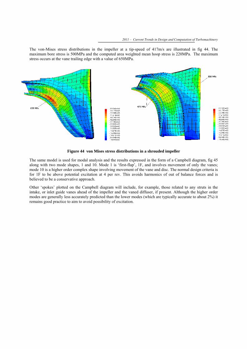
An integrated approach to the aero-mechanical optimisation … · ABSTRACT: The design of...

2011 – Current Trends in Design and Computation of Turbomachinery

An integrated approach to the aero-mechanical

optimisation of turbo compressors Chris Robinson, Mick Casey and Ian Woods

PCA Engineers Limited www.pcaeng.co.uk

ABSTRACT: The design of turbomachinery for high-technology products such as gas turbines, turbochargers and large industrial machinery has always embraced the latest analysis techniques to ensure that new designs reach higher levels of aerothermal performance with acceptable mechanical integrity. The challenge to maximize performance remains, but over the last decade, new issues have come to prominence to rival the fluid and structural aspects. Emphasis is now placed on the ability to design more nearly ‘right-first-time’ at low cost to shorten product entry into service and to further improve competitiveness. The present topical issues are numerical optimization, inclusion of more detail in the simulations and the more complete integration of the computational fluid dynamic (CFD) design process with preliminary aerodynamic design and with finite element (FE) mechanical analysis techniques. This paper describes an integrated turbomachinery design system applied to the design of centrifugal turbocompressors that can be applied in an optimizing environment. It explains in some detail the preliminary design approach where significant improvements have been made over recent years. Examples drawn from industry are used to illustrate the current state of art of CFD and FE as applied to turbochargers and industrial compressors. Keywords: Turbomachinery, compressor, turbocharger, gas turbine, throughflow, CFD, Finite Element

1. INTRODUCTION

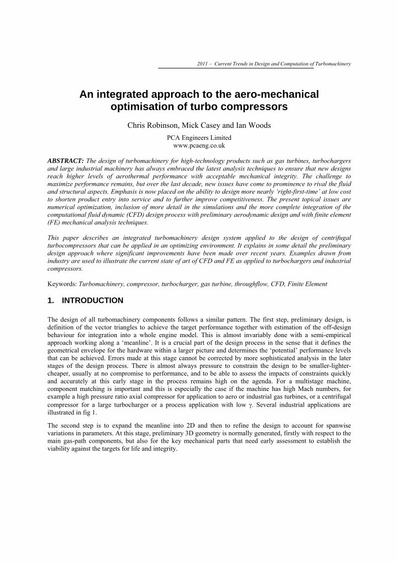
The design of all turbomachinery components follows a similar pattern. The first step, preliminary design, is definition of the vector triangles to achieve the target performance together with estimation of the off-design behaviour for integration into a whole engine model. This is almost invariably done with a semi-empirical approach working along a ‘meanline’. It is a crucial part of the design process in the sense that it defines the geometrical envelope for the hardware within a larger picture and determines the ‘potential’ performance levels that can be achieved. Errors made at this stage cannot be corrected by more sophisticated analysis in the later stages of the design process. There is almost always pressure to constrain the design to be smaller-lighter-cheaper, usually at no compromise to performance, and to be able to assess the impacts of constraints quickly and accurately at this early stage in the process remains high on the agenda. For a multistage machine, component matching is important and this is especially the case if the machine has high Mach numbers, for example a high pressure ratio axial compressor for application to aero or industrial gas turbines, or a centrifugal compressor for a large turbocharger or a process application with low γ. Several industrial applications are illustrated in fig 1.

The second step is to expand the meanline into 2D and then to refine the design to account for spanwise variations in parameters. At this stage, preliminary 3D geometry is normally generated, firstly with respect to the main gas-path components, but also for the key mechanical parts that need early assessment to establish the viability against the targets for life and integrity.

ČKD Nové Energo & TechSoft Engineering & Asociace strojních inženýrů ČR

Figure 1 Examples of centrifugal compressors in industrial applications

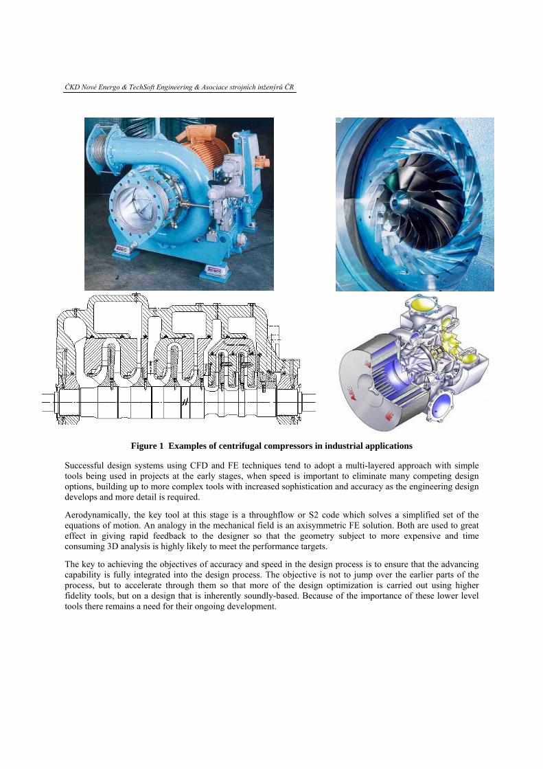
Successful design systems using CFD and FE techniques tend to adopt a multi-layered approach with simple tools being used in projects at the early stages, when speed is important to eliminate many competing design options, building up to more complex tools with increased sophistication and accuracy as the engineering design develops and more detail is required.

Aerodynamically, the key tool at this stage is a throughflow or S2 code which solves a simplified set of the equations of motion. An analogy in the mechanical field is an axisymmetric FE solution. Both are used to great effect in giving rapid feedback to the designer so that the geometry subject to more expensive and time consuming 3D analysis is highly likely to meet the performance targets.

The key to achieving the objectives of accuracy and speed in the design process is to ensure that the advancing capability is fully integrated into the design process. The objective is not to jump over the earlier parts of the process, but to accelerate through them so that more of the design optimization is carried out using higher fidelity tools, but on a design that is inherently soundly-based. Because of the importance of these lower level tools there remains a need for their ongoing development.


3D Aero 3D FE

Figure 2 Modern integrated turbomachinery design system

The simple tools also require a seamless integrated link from the preliminary design process to both the CFD analysis and the mechanical analysis. Fig 2 describes the integrated design system in use at PCA which is based around ANSYS Workbench and several in-house codes, part of the Vista suite.


2. MEANLINE DESIGN AND PERFORMANCE PREDICTION

2.1 1D Design point development

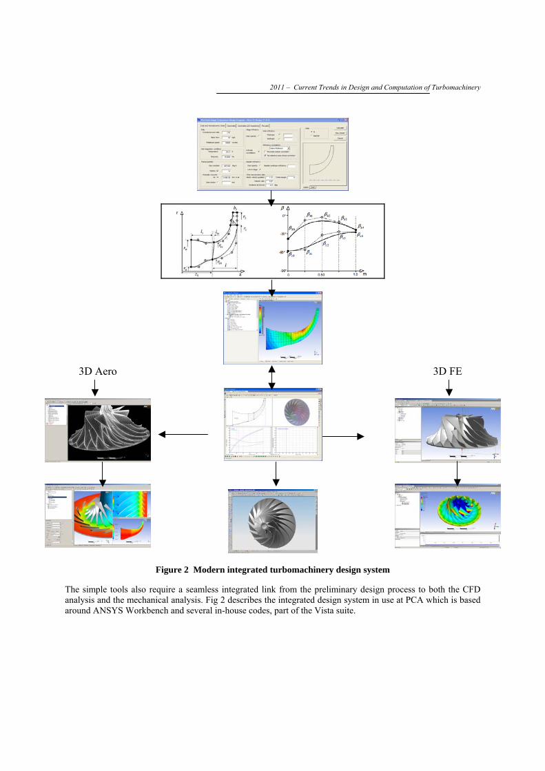
The design of a compressor stage normally is presented with targets for pressure ratio at a volume or mass flow and often constraints in terms of power (or efficiency) size and shaft speed. The pressure ratio (Π) can be written in terms of the ratio of specific heats (γ), work coefficient (ΔH/U2 = λ), isentropic efficiency (η) and the tip-speed Mach number (Mu) as follows:

( )1

222

2

11−

⎥⎦

⎤⎢⎣

⎡ Δ−+=Π

γγ

ηγ uMU

H

where the tip speed Mach number is given by t122 / RTUMu γ= . Fig 3 shows the variation in pressure ratio with tip speed Mach number for a typical range of radial impeller work coefficients from 0.6 to 0.8 for air with γ = 1.4 and an assumed efficiency of 86%.

Figure 3 Influence of Mach number and work coefficient on pressure ratio

So according to fig 3, the target pressure ratio more or less fixes the tip-speed for a given gas and inlet conditions; then the compressor must be sized appropriately for the inlet volume flow. The flow coefficient (φt1) is given by:

222

11 uD

Vtt

&=φ

and the value of φt1 strongly affects the likely efficiency of the compressor. This may effectively be a constraint, if the shaft speed is given and the required tip-speed is implied by the pressure ratio, the tip diameter is also relatively constrained.


At the preliminary design phase an empirical approach can be applied which simply correlates efficiency measurements on similar machines with global parameters such as specific speed or flow coefficient, size and clearance level. Two well-known correlations of this type are those of Casey and Marty (1985) and those of Rodgers (1980), both given by Cumpsty (2006). The former gives an estimate for the total-total polytropic stage efficiency of industrial shrouded stages (up to tip-speed Mach numbers of 1.0) and the latter the total-total isentropic impeller efficiency at higher tip-speed Mach numbers. Both represent more or less the state of the art that could be achieved at the time of publication with fairly large impellers (>300 mm), good diffusing systems and close attention to minimising all clearance gaps. Casey and Robinson (2007) have merged these two correlations into a more general form:

),( 21 utp Mf φη =

and taking account more recent experience of impellers designed with modern CFD methods, which leads to slightly higher peak efficiencies and a reduced rate of fall of efficiency with higher flow coefficient, fig 4.

0.50

0.55

0.60

0.65

0.70

0.75

0.80

0.85

0.90

0.00 0.05 0.10 0.15

Flow Coefficient

Poly

trop

ic E

ffici

ency

Mu=1.0Mu=1.2Mu=1.4Mu=1.6Mu=1.8Mu=0.8

Figure 4 Correlation between efficiency and stage flow coefficient and impeller Mach number

In the first instance the basic efficiency curve for a tip-speed Mach number of Mu=0.8 is defined. This curve is similar to that given by Casey and Marty (1985) and assumes a Reynolds number, Re = 0.8 x 106 and a roughness level, Ra = 3.6 x 10-6 m. The impellers are also assumed to have low clearance level (2% of exit channel height) and vaned diffusers. The basic equation for the variation of polytropic efficiency with flow coefficient at Mu = 0.8 is


( ) ( )[ ]

0.5000,0.27,08.0,86.01,08.0

21maxmax

41max2

21max1max1

====

−−−−=<

kkkk ttpt

φη

φφφφηηφ

( )[ ]0.10,08.0,86.0

1,08.0

3maxmax

2max13max1

===

−−=≥

k

k tpt

φη

φφηηφ

The modification to this curve to give an efficiency drop for higher tip Mach numbers is based on the work of Rodgers (1992) using a quadratic function. The best polytropic stage efficiencies that can be reached today are typically around 86 to 88%, depending on the size of impeller, the quality of the diffuser, the clearance levels and the level of expenditure and effort on development tests. Such good efficiencies are found in impellers designed for a flow coefficient in the range 0.06 ≤ 1tφ ≤0.09. If the designer has control over the shaft speed then a clear objective is to manipulate the design of the stage into this ‘sweet spot’. However, many modern machines are constrained either by synchronous speeds or by limitations constrained by direct drive electric motors and many designs are carried out at lower than optimum flow coefficients.

Low flow coefficient stages ( 1tφ < 0.05) have inherently lower efficiency because of narrow channels with small hydraulic diameters leading to higher frictional losses. In addition, parasitic losses (disc friction and leakage losses) increase as the flow coefficient decreases (as they become a larger part of the total energy input of the stage). Very high flow coefficient stages ( 1tφ > 0.09) have lower efficiencies than those at the optimum flow coefficient because of the high gas velocities and high Mach numbers that occur. It is simply not possible to increase the impeller inlet eye diameter of a radial wheel much above 80% of that of the impeller outlet, as this dilutes the useful effect of radius change on pressure rise, so this constrains the inlet area available leading to high inlet velocities at high flow coefficients.

Having established a baseline level of polytropic efficiency, this is corrected for the effects of Reynolds number and tip clearance in the case of open wheels. The effect of clearance is roughly 1% change in stage efficiency for 2% change in the ratio of impeller axial clearance to exit channel width.

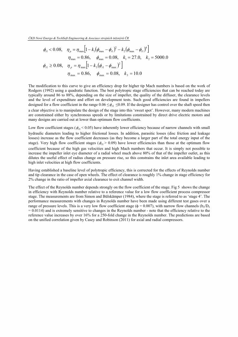
The effect of the Reynolds number depends strongly on the flow coefficient of the stage. Fig 5 shows the change in efficiency with Reynolds number relative to a reference value for a low flow coefficient process compressor stage. The measurements are from Simon and Bülskämper (1984), where the stage is referred to as ‘stage 4’. The performance measurements with changes in Reynolds number have been made using different test gases over a range of pressure levels. This is a very low flow coefficient stage (φ = 0.007), with narrow flow channels (b2/D2 = 0.0114) and is extremely sensitive to changes in the Reynolds number - note that the efficiency relative to the reference value increases by over 16% for a 250-fold change in the Reynolds number. The predictions are based on the unified correlation given by Casey and Robinson (2011) for axial and radial compressors.


Figure 5 Correction to compression efficiency for change in Reynolds number

The impeller vane shape at outlet is superficially similar for all modern impellers, as it is now commonplace to make use of back-sweep to enhance the operating stability of the stage. Considering the outlet velocity triangle of the impeller, the work input (λ) is a function of the vane exit relative gas angle (β2) and the outlet flow coefficient (φ2 = Cm2/U2):

22 tan1 βφλ −=

For an impeller with radial blades theoretically giving purely radial outflow (β2 = 0) the work input is constant with flow. If the efficiency were to remain constant with flow rate then the slope of the pressure rise characteristic with flow would correspond to that of the work input. To avoid surge and rotating stall it is necessary for the stage to have a falling pressure rise characteristic with increasing flow, and so back-sweep is used to provide an inherently stable form of characteristic with rising pressure as the flow is reduced. Generally an increase in backsweep leads to more surge margin, moving the locus of peak efficiency away from the surge line. The only downside is that as shown in fig 3, the backswept impeller with a lower value of ΔH/U2 needs a higher tip-speed to achieve the target pressure ratio and consequently has higher stress. This can have implications for the selection of materials, typical values for the tip-speeds of impellers are:

• Cast Aluminium: 200 to 300m/s • Forged aluminium up to 450 to 500m/s • Steel: 350 to 500 m/s (open), 280 to 340m/s (shrouded) • Titanium alloys: 500 to 700m/s

Even under ideal frictionless conditions the flow leaving the impeller is not perfectly guided by the blades and this effect is best modeled in radial compressors by the use of a slip velocity (cs) and the equation for work input is modified to be:

222

tan1 βφλ ′+−=ucs


where β'2 denotes the vane angle. This relatively simple concept, analogous to deviation in axial compressors. For practical purposes a good rule of thumb is the so-called Wiesner correlation, which is based on experimental data and theoretical analysis of Wiesner (1967), with a simple expression for the non-dimensional slip velocity of

7.02

2

cos

bl

s

Zuc β ′

=

For stages of moderate backsweep, the correlation between Wiesner and experiment is very good, fig 6.

Figure 6 Impeller exit velocity triangles and the Wiesner correlation

The variables that are under the control of the designer are usually studied parametrically and this is most effectively carried out by a simple 1D code such as VistaCCD, fig 7. Such codes will include the effects described above and further enhancements such as more detailed treatment of the inducer at hub, mid-span and shroud, including the effects of choking, and consideration of real gases. The designer will typically consider variation of the backsweep angle, the extent of diffusion within the impeller passage (the stage reaction). In addition to pursuing the highest achievable stage efficiency, consideration is also given to the absolute frame conditions leaving the impeller, ie the diffuser inlet conditions.


Figure 7 VistaCCD 1D preliminary design calculation

For a vaned diffuser, the optimum is normally to push up the stage reaction until the diffuser inlet absolute gas angle is in the range 70-75°, provided that the impeller shroud diffusion is not excessive. In the case of a vaneless stage, the flow must typically leave the impeller at an angle of 60-70°, with higher dynamic head, to avoid excessive spiral path length in the diffuser.

On completion of the parametric study, the flow conditions at inlet and outlet of the impeller are known. The geometry at the 4 corner points describing the impeller at inlet and outlet is also known. The channel and vane angle distribution within the impeller is developed in section 3 below, with a starting guess as shown in the thumbnail in fig 7. Vista CCD exports data in a format useful for Vista GEO, PCA’s in-house vane development tool, and ANSYS BladeGen.

2.2 1D Performance map prediction

An important requirement during the preliminary design of a compressor stage is the calculation of a reliable performance map as a guide to the expected operating flow range and the sensitivity to speed variations when the design is completed. With this information the designer can assess if the design will be suitable for the application. For example, it is possible to check if a new design will provide adequate efficiency, pressure ratio and surge margin on the low speed characteristics and sufficient choke margin at high speeds. For a gas turbine application, it is important in the assessment of whether the engine can be started without surging the compressor.

The approach described below is based on the fact that well-designed compressor stages for a particular aerodynamic duty tend to have fundamentally similar shapes of their efficiency performance maps. This indicates that the duty itself is very good guide to the form of the performance map. The method uses four key non-dimensional parameters at the design point to determine the performance map, rather than the geometry of the stage:

• The expected design point polytropic efficiency, η • The global volume flow coefficient, φ • The stage work coefficient, λ • The stage tip-speed Mach number, M


If this design is done well then the performance characteristic for this optimally designed stage can be implied from these design values. This has obvious advantages in terms of delivery of the map at an early point in the design cycle of the complete machine so any potential shortfall can be addressed before significant expenditure of time and cost.

The same approach is used at PCA for all classes of radial flow machine, turbochargers (high specific flow, vaneless diffusers) to low flow coefficient industrial stages with vaned diffusers. The different classes of machine simply use alternative empirical coefficients in the equations. The parameterised system of algebraic functions can be adapted to other gases and to generate a stage-stacking tool for multi-stage process compressors.

The objective is to calculate the values of two dependent variables (the polytropic efficiency and work coefficient) for specific values of the independent variables (the flow coefficient and tip-speed Mach number):

),(, Mf φλη =

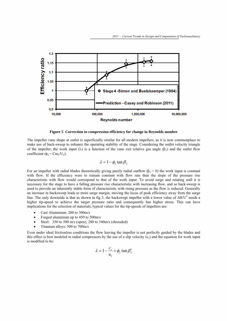
Rodgers introduced the concept of establishing normalised shapes of characteristics, although he used choke flow whereas the present approach is based on the design flow, fig 8a, for example.

DD /1

/ ⎥⎤

⎢⎡

⎟⎞

⎜⎛ φφη

0

0.1

0.2

0.3

0.4

0.5

0.6

0.7

0.8

0.9

1

0 0.2 0.4 0.6 0.8 1 1.2 1.4 1.6 1.8

η/ηp

φ/φp

0.50.811.11.21.31.41.51.6

0.1

0.2

0.3

0.4

0.5

0.6

0.7

0.8

0.9

1.0

0.4 0.6 0.8 1.0 1.2 1.4 1.6 1

η/ηp

.8

φ/φp

0.41Mu=0.4100.55Mu=0.5500.686Mu=0.6860.825Mu=0.8250.962Mu=0.9621.1Mu=1.1001.235Mu=1.2351.37Mu=1.3711.51Mu=1.510

a) form of the normalised efficiency vs flow curves b) validation of a turbocharger compressor

Figure 8 Normalised curves describing the variation of efficiency with flow and Mach number

The equations used to describe these curves are not a real physical model of the losses but a particular structure has been chosen in order to reproduce important physical effects in the stage characteristics. In the current work the variation of stage efficiency with flow along a speed line is a modified form of an elliptic curve:

2/12

2

2

2

2

1,1⎥⎥⎦

⎤

⎢⎢⎣

⎡⎟⎠⎞

⎜⎝⎛−==+

by

ax

by

ax

For flows below the peak efficiency point this equation is modified to have a variable exponent to give the characteristic curves for efficiency ratio as a function of flow ratio as follows:

cp

c

pp /

11,⎥⎦

⎢⎣

⎟⎠

⎜⎝

−−=<φφη

φφ


A similar equation is used for flows below peak efficiency. The variable exponent takes into account the fundamentally different shapes of efficiency characteristics for low Mach number and high Mach number impellers. Low Mach number impellers tend to have a smooth drop in efficiency ratio related to incidence losses as the flow increases above peak efficiency. High Mach number stages tend to have a small plateau of high efficiency close to the peak efficiency point and then drop much more sharply into choke.

Having defined the equations the coefficients were derived based on analysis of more than 45 different compressor stages covering the full range of applications. The typical agreement using these fixed set of coefficients is shown in fig 8b giving variations of efficiency ratio with flow ratio for a typical turbocharger stage with a vaneless diffuser.

Experience shows that the operating range of compressors is largest at very low Mach numbers and remains constant at low Mach numbers. The range then decreases with increasing Mach number but again remains more or less constant at much higher Mach numbers. This is illustrated by fig 9, for turbocharger-style impellers where the choke flow is defined by the choke of the impeller inlet. The differences are related to the different throat areas, blade thicknesses and shroud diameter of the different impellers.

0.4

0.5

0.6

0.7

0.8

0.9

1

0.4 0.6 0.8 1 1.2 1.4 1.6 1.8 2

φp/φc

M

turbocharger-vaneless

test data

Figure 9 Range between peak efficiency and choke over a range of Mach number

The flow coefficient at the peak efficiency point tends to increase as the tip speed Mach number increases. This is caused partly by the effect of the change in the density on the velocity triangles at impeller inducer inlet with speed. It is also related to the mismatch with the diffuser as this becomes too small for the impeller at low speeds forcing the peak efficiency of the stage to move to a lower flow coefficient.

It is interesting to compare the range capability of vaned and vaneless diffuser stages using a presentation analogous to the ‘α-Mn’ diagram used to visualize the available operating range of compressor cascades at varying incidence and flow Mach number levels in the preliminary design of axial compressors, see the examples given by Casey (1994). Fig 10a shows the variation of the choke flow coefficient, the peak efficiency flow coefficient and the surge flow coefficient as a function of the tip-speed Mach number for the typical vaneless diffuser turbocharger stage, and fig 10b shows this variation for a turbocharger stage with a vaned diffuser. In both cases the flow coefficients are normalized relative to the flow coefficient that would occur at peak efficiency at low Mach number, φp0, which is lower than the design flow coefficient.


0

0.5

1

1.5

2

2.5

0 0.5 1 1.5 2

φ/φpo

M

φ ‐Mach Diagram for vaneless diffusers

phi_c/phi_p0

phi_c/phi_p0

phi_p/phi_p0

phi_p/phi_p0

phi_s/phi_p0

phi_s/phip0

0

0.5

1

1.5

2

2.5

0 0.5 1 1.5 2

φ/φpo

M

φ ‐Mach Diagram for vaned diffusers

phi_c/phi_p0

phi_c/phi_p0

phi_p/phi_p0

phi_p/phi_p0

phi_s/phi_p0

phi_s/phip0

a) φ – Mach diagram for vaneless diffusers b) φ – Mach diagram for vaned diffusers

Figure 10 Variation in range with Mn for stages with vaneless and vaned diffusers

The difference between these two diagrams also shows up some interesting aspects related to the effect of matching on the characteristics at different speeds. Firstly, the much wider range of stages with vaneless diffusers can be seen from the spacing between the surge and choke lines in these diagrams (fig 10a). Secondly the shift in the flow coefficient at the peak efficiency point with Mach number is very different for the two cases. In the vaned diffuser case, fig 10b, the diffuser is generally matched to the impeller at high speeds and then becomes much too small at low speeds. This causes the impeller to operate at high incidence and forces the stage characteristic to move to a lower flow coefficient. This effect is much less strong in the vaneless diffuser. A vaneless diffuser with no blades can accept higher flows at lower speeds as it does not choke and the impeller is not forced to operate at such a low flow coefficient.

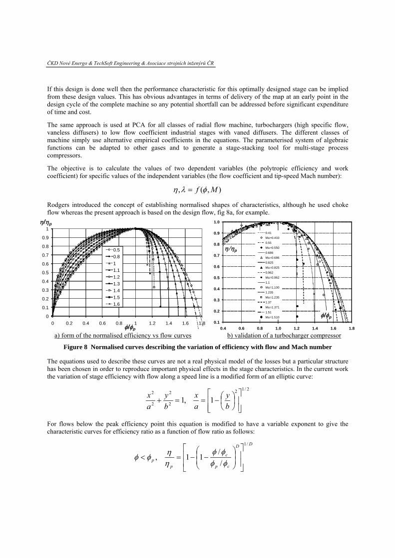
Fig 11 compares the predicted and the measured characteristics of a typical turbocharger compressor stage with a vaneless diffuser over a range of speeds. The measured characteristics were obtained on a turbocharger gas stand using a small compressor impeller with a back-sweep of approximately -30° over a range of speeds from 40,000 to 230,000 rpm. The measured points on all speed lines agree very well (to within ± 2%) with the predictions, and the measured surge line lies typically between the limits of the predicted pessimistic and optimistic lines.

The design point of this stage is denoted as a large open circle on the third fastest speed line. The non-dimensional values of the four key parameters and the impeller diameter have been specified at this condition and all other curves are then calculated from this point using the approach outlined above. In addition to these non-dimensional coefficients, the slip factor, the degree of reaction and the disc friction coefficient are specified, whereby standard values from other impellers may be used if these are not known, but no other information on the geometry is needed. As this compressor stage has been tested in a turbocharger with heat transfer from the turbine, the efficiency shown here includes a correction for the effect of heat transfer according to the approach of Casey and Fesich (2010). Without this correction the apparent peak efficiency would not drop sharply as the speed decreases as shown in fig 11. The curves also include an extrapolation to a higher rotational speed, which was not measured, to demonstrate that the system still produces sensible characteristics at higher speeds.


1.00

1.50

2.00

2.50

3.00

3.50

4.00

4.50

0.000 0.020 0.040 0.060 0.080 0.100 0.120 0.140

π

Inlet volume flow m3/s

0.41M=0.4100.55M=0.5500.686M=0.6860.825M=0.8250.962M=0.9621.1M=1.1001.235M=1.2351.371M=1.3711.51M=1.5101.65

0.00

0.20

0.40

0.60

0.80

0.000 0.020 0.040 0.060 0.080 0.100 0.120 0.140

ηs

Inlet volume flow m3/s a) Pressure ratio vs Mu and flow b) Efficiency vs Mu and flow

Figure 11 Predicted characteristic for a turbocharger compressor stage with vaneless diffuser

This method is routinely used as VistaCCM. An obvious limitation is that it only considers the global performance data and not the component losses (impeller, diffuser and volute) which are the cause of this behavior. The procedure suggested by Rodgers (1964) and used by Swain (1990) is applied as a refinement for vaned diffusers where the use of separate diffuser and impeller characteristics allows the designer to identify in more detail the choking and instability limits of each component and to study changes in component matching with speed. It is especially useful where the designer may wish to exploit mis-matching at one speed to enhance range at another. This refinement (Vista CCP) is used in the optimisation of vaned diffusers for higher pressure turbochargers and process compressors.

3. DEVELOPMENT OF THE DESIGN IN 2D

3.1 Parameterise the geometry

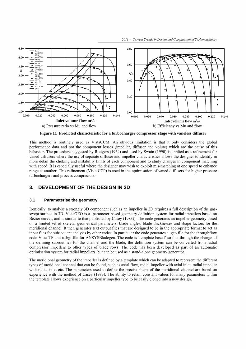
Ironically, to analyse a strongly 3D component such as an impeller in 2D requires a full description of the gas-swept surface in 3D. VistaGEO is a parameter-based geometry definition system for radial impellers based on Bezier curves, and is similar to that published by Casey (1983)). The code generates an impeller geometry based on a limited set of skeletal geometrical parameters, blade angles, blade thicknesses and shape factors for the meridional channel. It then generates text output files that are designed to be in the appropriate format to act as input files for subsequent analysis by other codes. In particular the code generates a .geo file for the throughflow code Vista TF and a .bgi file for ANSYSBladegen. The code is ‘template-based’ so that through the change of the defining subroutines for the channel and the blade, the definition system can be converted from radial compressor impellers to other types of blade rows. The code has been developed as part of an automatic optimisation system for radial impellers, but can be used as a stand-alone geometry generator.

The meridional geometry of the impeller is defined by a template which can be adapted to represent the different types of meridional channel that can be found, such as axial flow, radial impeller with axial inlet, radial impeller with radial inlet etc. The parameters used to define the precise shape of the meridional channel are based on experience with the method of Casey (1983). The ability to retain constant values for many parameters within the template allows experience on a particular impeller type to be easily cloned into a new design.


The impeller blade is defined as a ruled surface of straight lines joining points on the hub and the shroud contours that are equidistant along the meridional channel of the impeller, between the leading edge, the splitter leading edge and the trailing edge. The hub and shroud blade sections are defined as a distribution of camber line and thickness specified as Bezier functions along the meridional length, whereby the leading edge and trailing edge radii are defined as separate parameters. An option has been included which allows the hub blade angle distribution to be modified internally by the code to achieve a specified lean (typically 0°) of the leading edge and a specified rake angle at the trailing edge. This makes use of the user-defined hub angle distribution as a guide but overwrites this within the blade row, keeping the inlet and the outlet blade angles the same.

The meridional channel geometry definition begins with the 1D method described above, Vista CCD. Key skeletal parameters are therefore already fixed for the preliminary design optimisation process, and do no longer need to be changed during the subsequent design process.

Figure 12 Parameterised description of an impeller geometry

Fig 12 shows the parameterised meridional channel and vane angle and thickness distributions. These can be adjusted manually or randomly varied during the optimisation process as described below. An output format available is the so-called ‘meanline’ description of the gas-swept surface as a series of (r, θ, z, tn) descriptions of the vane camberlines, .rtzt in ANSYS BladeGen format.

The same geometry system can be applied to all components through the stage: inlet, impeller, diffuser (vaned or vaneless), cross-over and vaned return channel and files can be linked together to define a full stage (or stages) in a single run. Fig 13 shows some key dimensions for the parameterised stage.


Figure 13 Parameterised geometry of a complete centrifugal compressor stage

3.2 2D Throughflow analysis

Although the flow in turbomachinery is three-dimensional (3D) and analysis in 3D has become relatively routine, the design process has relied on simplifying the problem by considering the flow on two sets of intersecting surfaces; blade-to-blade (S1) and the mean stream surface (S2) as shown in fig 14 for an axial row for clarity.

Figure 14 Intersecting S1-S2 surfaces in a bladerow

Design is typically accomplished by a predictor-corrector or ‘design by analysis’ approach and this remains the only practicable approach to define the flow path geometry that can subsequently be more fully analysed using 3D CFD.


The designer essentially sets the vector-triangles for each bladerow using first 1D then 2D techniques, then defines hardware that is expected to reflect these boundary conditions and deliver the target performance. The hardware is then analysed, the results are assessed to check compliance with the vector-triangle boundary conditions. The geometry is then revised and the process repeated until satisfactory convergence is obtained.

Solution on the mean stream surface (S2) is one of the most enduring elements of the turbomachinery design system. It remains the basis of all multistage compressor and turbine designs, even in the market segments investing most heavily in new simulation technology such as aero and industrial gas turbines. It provides the definitive, reference performance model and reference point for the subsequent detailed design of each bladerow.

The position of throughflow tools to define the boundary conditions of new designs seems assured. In developing the hardware to meet the boundary conditions, the designer needs rapid feedback to establish a feel for the parameters controlling the aerodynamic behaviour of each component. 3D CFD can provide this feedback, though for most users not with adequate turnaround: solutions per bladerow are necessary in seconds, or at worst minutes, for optimal development.

Sophisticated, coupled S1-S2 solution systems (an iteration between blade-to-blade, S1 and throughflow, S2) were also developed in the 1980’s. S1-S2 methods generally work well if the flow is reasonably well-behaved and follows the meridional stream surfaces. For more sophisticated components, high Mach number transonic fans for aero engine application for example, S1-S2 has been superseded as an analysis tool by 3D CFD which is more straightforward to set up and run and is inherently less reliant on semi-empirical correlations. In high solidity radial compressor and pump applications, however, a simplified S1-S2 system has been used, in which the mean camber line is taken to represent the S2 stream surface and in which the variation in the blade-to-blade flow is taken to be linear (Casey and Roth, 1984). This still has a useful position in an integrated design system through its adequate representation of the physics and its speed of computation. VistaTF (Casey and Robinson, 2010) is based on this approach and the remainder of this paper illustrates its application to centrifugal compressor design.

3.3 Basic description of throughflow analysis

The grid for the calculation is based on fixed calculating stations, which are roughly normal to channel walls, and the streamlines of the mean circumferentially-averaged flow in the meridional direction, such as fig 15.

leading edge q-o duct q-o

trailing edge q-o

internal rotor q-o internal stator q-o

inlet q-o outlet q-o

streamlines

leading edge q-o duct q-o

trailing edge q-o

internal rotor q-o internal stator q-o

inlet q-o outlet q-o

streamlines

Figure 15 Generalised throughflow calculation mesh


The meridional streamline grid is not fixed, apart from the hub and shroud streamlines on the annulus walls, but changes continually during the iterations. The fixed calculating stations are oriented with the leading and trailing edges, so need to be curved if these are curved, and can be in duct regions, that is in the blade-free space upstream and downstream of blades, at the leading and trailing edges of the blades and internally within the blades.

The blade geometry is described in an (r, θ, z) polar coordinate system and uses blade lean angles (γ) to the axial and radial directions at all points on the calculation mesh within bladerows. Calculation of the lean angles (γz and γr) is performed automatically within ANSYS Workbench or by a standalone program (RTZTtoGEO). The (r, θ, z, tn) ‘meanline’ description of blade geometry is more or less industry standard and is an export from BladeGen with extension .rtzt.

By suitable combinations of different types of calculating station any type of turbomachine can be modelled. These can be simple ‘isolated bladerow’ cases normally used during the design iterations (fig 16a) or more sophisticated, full stage calculations such as fig 16b. The variable plotted is the meridional velocity (cm) the vector sum of the axial and radial components. It is the gradient of this parameter that is the subject of the radial equilibrium equation.

NASA 10pps 7:1 impeller Multistage industrial compressor

Figure 16 Typical calculation meshes for VistaTF

Flow does not, by definition, cross the streamlines so the mesh at the end of the iterative process gives the designer an impression of the flow-field. Where the streamlines are close together, the velocities are higher (close to the casing for example) and far-apart streamlines denote low velocities, flow may be tending towards separation.

Vista TF solves a simplified set of equations that are derived from the same equations solved by any CFD method. In simple terms these are:


• Continuity of mass • Conservation of energy • Equation of state • Inviscid momentum equation for the flow on the mean stream surface ’Mean stream surface’ means, in this context, the circumferentially averaged stream surface, ie there is no variation of parameters in the S1 or blade-to-blade direction.

The energy equation combines the first law of thermodynamics and the Euler equation which relates the change in total enthalpy across a bladerow to the change in angular momentum. The momentum equation is expressed in terms of the spanwise gradient of meridional velocity along a calculating station, a generalised form of the radial equilibrium equation (fig 17a).

q

cm

dqdcm

321 mmm &&&

q

q

cm

dqdcm

321 mmm &&&

q

a) Radial equilibrium equation b) Iterative solution process Figure 17 Equilibrium equation and its solution

To start the solution process, the meridional streamlines are approximated by splitting the flow into regions of equal area, then a first guess is made of all parameters: • ht from the Euler equation • s from loss correlations • ρ from ht and s Then the distribution of meridional velocity (cm) is determined (fig 17b): • the gradient of the meridional velocity (dcm/dq) from general radial equilibrium • the level of the meridional velocity from the continuity equation cm is adjusted on the mean streamline until both gradient and mass flow are satisfied. Based on the revised cm distribution, the estimate of the streamline positions can be revised, then the process iteratively repeated until cm and all other parameters are converged

Although the method is based around a mean stream surface, it includes (effectively as a post-processing option) a linearised blade-to-blade solution due to Stanitz and Prian (1951).

mrccp u

m ∂∂

=∂∂

−)()(ρ

θ


At each meridional position, this equation can be integrated to give Δp and then the suction and pressure surface values found from p ± Δp and then these values used to estimate the respective Mach numbers.

Aerodynamic boundary conditions can be applied in a variety of forms: • Inlet conditions, for eg P0, T0, α0 • Dimensional operating conditions such as shaft speed and mass flow; • Non-dimensional operating conditions such as machine Mach number (Mu2) and inlet flow coefficient

(φt1=Vt1/U2D2 ). 2

In common with all S2 throughflow methods, the user must also define the ‘loss and turning’ for each blade row. For a centrifugal compressor these are usually via a constant polytropic efficiency (ηp) and the Wiesner correlation for slip factor.

A full description of the method is available in the open literature (Casey and Robinson 2010).

3.4 Strengths and limitations of throughflow analysis

3.4.1 Strengths

In an integrated design system workflow the throughflow approach sits downstream of the 1D design (Vista CCD) and to some extent alongside CFD (CFX) as illustrated by the schematic programme in fig 18.

Figure 18 Throughflow integrated into the design programme

Its primary function is to permit rapid development of the vane shape by providing feedback on the aerodynamic ramifications of modification to vane shape defined by the user in VistaGEO or ANSYS BladeGen. This should ensure that geometry taken through the more time consuming, full-3D CFD analysis route is not only viable in terms of basic performance parameters, such as work input (λ = ΔH/U2), but also incorporates the user’s background knowledge on what makes for a good aerodynamic design. What throughflow delivers for the user includes: • feedback in almost real-time, order of seconds, for a single row analysis; • accurate representation of flows dominated by curvature effects; • predicted Mn distributions at hub, mid-span and shroud locations; • warnings of possible problems with choke; • suitability of splitter location; • predicted work input (ΔH/U2) taking account of vane angles and rake; • accurate assessment of incidence across the span of the vanes; • distribution of vane loading parameters for comparison with experience; • possibility of automated optimisation.


Throughflow can best be appreciated as a productivity enhancement and as a means to capture past experience in a rational way.

Figure 19 Design without throughflow support

Fig 19 shows an alternative version of fig 18 where the vane shape is developed only with feedback from CFD. The overall length can be expected to be protracted since there is no filtering of non-viable designs ahead of detailed CFD as offered in fig 18. This means an increased elapsed time and corresponding impact on computing resource. It is also more difficult to diagnose possible reasons for performance shortfall in early design iterations. The throughflow results give a background understanding of the flow within the component that can lead the engineer towards and accurate interpretation of what is occurring and how to effect changes on the next iteration.

3.4.2 Limitations

It is important to appreciate that throughflows in general cannot offer the user information on: • direct prediction of efficiency (ηp is a user-input parameter)a; • surge line and choke limits in detail, hence map predictionb; • viscous flow phenomenac; • flow phenomena driven by secondary effects such as clearancec • transient effectsc. Notes: a To predict efficiency directly would require sophisticated semi-empirical modelling through correlations. While this is included in axial machinery throughflow codes, it is felt that the phenomena within centrifugal machines are more complex and best captured by subsequent CFD analysis. If correlations are used, these are notorious for the extent of input parameters that are required, many of which are not known in detail at this stage in the design process, and are ultimately only really useful if the scope of the design is interpolative, i.e. within a known and well-validated technology base. b Surge is well-known as the performance parameter least amenable to prediction by more detailed analysis such as 3D CFD. It can be achieved using the meanline performance prediction tools described earlier. c These effects are excluded from steady-state throughflow analysis by definition, they are well-captured by higher level 3D CFD analysis.

3.5 Application of throughflow analysis

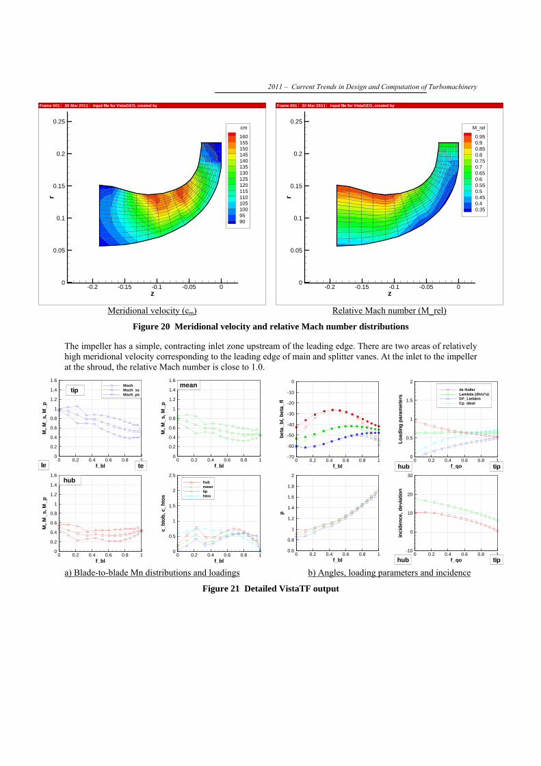
Considering a centrifugal compressor stage of pressure ratio 2.5 in air with moderate specific flow (φ=0.095) and impeller Mu2 of 1.15. The impeller has high backsweep (50°) and a work coefficient (ΔH/U2) of 0.66. The impeller is non-dimensionally similar to that found in a turbocharger or a single-stage industrial compressor. Vista TF predictions are shown in figs 20 and 21 for a reasonably well-optimised vane


z

r

-0.2 -0.15 -0.1 -0.05 00

0.05

0.1

0.15

0.2

0.25cm

1601551501451401351301251201151101051009590

Frame 001 ⏐ 30 Mar 2011 ⏐ Input file for VistaGEO, created by

z

r-0.2 -0.15 -0.1 -0.05 0

0

0.05

0.1

0.15

0.2

0.25M_rel

0.950.90.850.80.750.70.650.60.550.50.450.40.35


Meridional velocity (cm) Relative Mach number (M_rel)

Figure 20 Meridional velocity and relative Mach number distributions

The impeller has a simple, contracting inlet zone upstream of the leading edge. There are two areas of relatively high meridional velocity corresponding to the leading edge of main and splitter vanes. At the inlet to the impeller at the shroud, the relative Mach number is close to 1.0.

f_bl

M,M

_s,M

_p

0 0.2 0.4 0.6 0.8 10

0.2

0.4

0.6

0.8

1

1.2

1.4

1.6MachMach_ssMach_ps

tip

le te f_bl

M,M

_s,M

_p

0 0.2 0.4 0.6 0.8 10

0.2

0.4

0.6

0.8

1

1.2

1.4

1.6mean

f_bl

M,M

_s,M

_p

0 0.2 0.4 0.6 0.8 10

0.2

0.4

0.6

0.8

1

1.2

1.4

1.6hub

f_bl

c_bt

ob,c

_hto

s

0 0.2 0.4 0.6 0.8 10

0.5

1

1.5

2

2.5hubmeantiphtos

f_bl

beta

_bl,

beta

_fl

0 0.2 0.4 0.6 0.8 1-70

-60

-50

-40

-30

-20

-10

0

f_qo

inci

denc

e,de

viat

ion

0 0.2 0.4 0.6 0.8 1-10

0

10

20

30

hub tipf_bl

p

0 0.2 0.4 0.6 0.8 10.6

0.8

1

1.2

1.4

1.6

1.8

2

f_qo

Load

ing

para

met

ers

0 0.2 0.4 0.6 0.8 10

0.5

1

1.5

2de HallerLambda (dh/u*u)DF_LiebleinCp_ideal

hub tip

a) Blade-to-blade Mn distributions and loadings b) Angles, loading parameters and incidence

Figure 21 Detailed VistaTF output


Fig 21 shows more detailed output. Starting with the relative Mach number distribution along the shroud ((a) top left), the basic calculation yields the mean, central curve then Stanitz and Prian gives the off-set for both suction (upper) and pressure (lower) surfaces. The deceleration of the mean level is close to linear, design intent. The step change in Mach number reflects the doubling of the vane count at the splitter leading edge. Another important feature is the relatively small increase in the peak suction surface Mach number over the inlet value (1.05). Similar curves are also shown at mid and tip sections in green and red respectively. Note that at the hub (a) bottom left) there is a larger difference in the suction and pressure surface leading edge Mach number levels the effect of incidence.

The meridional distribution of blade-to-blade loading parameters ((a) bottom right) show very similar levels at mid and tip over the rear half of the vane, peaking at approximately 0.6. The hub is slightly higher at 0.7. This again reflects design intent, targeting a level of loading which can be most dramatically influenced by the vane count. In the inducer, the levels at mid and tip are lower, again design intent. If the loading is too high in the inducer then the vanes are at risk of premature stall. If the vanes are too lowly loaded, then efficiency will tend to be compromised as the wetted area is too high.

b) top left summarises the vane and gas angles on the three planes of interest, metal are solid and gas angles are dashed. The shroud vane angle shows very low turning in the inducer and it is this at the high level of Mach number that has resulted in the low peak Mach number discussed earlier.

b) top right shows some overall loading parameters, most important of which is the work coefficient (λ=ΔH/U2). This should reflect the target value set during the 1D design. It is also important to check the diffusion in relative Mach number at the shroud, the de Haller number. This should also match the design intent from the 1D analysis, avoiding excessive diffusion of the relative flow and consequent risk of separation.

b) bottom right shows the spanwise variation of incidence (red) and deviation, the result of the slip velocity (green). The incidence variation is about 10° hub to shroud, this is the outcome of designing a radially stacked vane at the inlet. The incidence should be low at the shroud, high incidence coupled with high relative Mach number will lead to excessive shroud Mach number in the inducer and premature stall. High incidence at the hub, of order 10° to 15° can be tolerated since the flow is not subject to much overall diffusion, the inlet and outlet Mach number are at similar levels. Ideally this would be reduced but the problem is that this results in a small throat area. For turbochargers, for example, a large throat area relative to the inlet size is desirable since this minimises the overall size and inertia for a given engine flow.

The following parameters are considered to have an effect on the efficiency: 1. Suction surface peak Mach number 2. Suction surface average Mach number 3. Minimum Mach number on pressure surface hub 4. Incidence at hub 5. Incidence at tip 6. Loading limit of inducer 7. Loading limit of rear part of impeller 8. Loading limit of the middle part of the impeller 9. Loading limit hub to shroud 10. Shape of mean shroud velocity distribution 11. De Haller number 12. Work coefficient 13. Flow angle into diffuser


These were weighted and included in the fitness function for a Breeder Genetic Algorithm (BGA) approach to the optimisation of impeller vanes (Casey, Robinson and Gersbach, 2008). VistaGEO provided the geometry with random variation of selected parameters within a range defined by the user.

If throughflow can be used effectively to result in an optimum vane and channel shape, it can also give a good insight into the effects of compromising the geometry. Fig 22 starts from the optimum solution with L/D of 0.30 and progressively reduces impeller length, a typical demand driven by rotordynamic constraints. As length reduces the potential effect of the axial to radial bend at the shroud becomes more significant, so the flow profile experienced across the span of the impeller at inlet is more pronounced.

z

r

-0.2 -0.15 -0.1 -0.05 00

0.05

0.1

0.15

0.2

0.25cm

1601551501451401351301251201151101051009590


z

r

-0.2 -0.15 -0.1 -0.05 00

0.05

0.1

0.15

0.2

0.25cm

1601551501451401351301251201151101051009590


z

r

-0.2 -0.15 -0.1 -0.05 00

0.05

0.1

0.15

0.2

0.25cm

1601551501451401351301251201151101051009590


f_bl

M,M

_s,M

_p

0 0.2 0.4 0.6 0.8 10

0.2

0.4

0.6

0.8

1

1.2

1.4


tip

le te f_bl

M,M

_s,M

_p

0 0.2 0.4 0.6 0.8 10

0.2

0.4

0.6

0.8

1

1.2

1.4


tip

le te f_bl

M,M

_s,M

_p

0 0.2 0.4 0.6 0.8 10

0.2

0.4

0.6

0.8

1

1.2

1.4


tip

le te

f_qo

inci

denc

e,de

viat

ion

0 0.2 0.4 0.6 0.8 1-10

0

10

20

30

hub tip f_qo

inci

denc

e,de

viat

ion

0 0.2 0.4 0.6 0.8 1-10

0

10

20

30

hub tip f_qo

inci

denc

e,de

viat

ion

0 0.2 0.4 0.6 0.8 1-10

0

10

20

30

hub tip L/D = 0.30 L/D = 0.25 L/D = 0.20

Figure 22 Varying impeller length

At L/D of 0.25, the incidence at the shroud is more negative and at the hub more positive, also the peak suction surface relative Mach number has increased from the inlet value of 1.0 to 1.2.


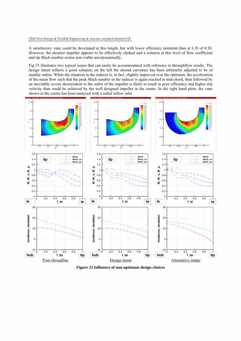
A satisfactory vane could be developed at this length, but with lower efficiency potential than at L/D of 0.30. However, the shortest impeller appears to be effectively choked and a solution at this level of flow coefficient and tip Mach number seems non-viable aerodynamically.

Fig 23 illustrates two typical issues that can easily be accommodated with reference to throughflow results. The design intent reflects a good solution; on the left the shroud curvature has been arbitrarily adjusted to be of smaller radius. While the situation in the inducer is, in fact, slightly improved over the optimum, the acceleration of the mean flow such that the peak Mach number in the inducer is again reached at mid-chord, then followed by an inevitably severe deceleration to the outlet of the impeller is likely to result in poor efficiency and higher slip velocity than could be achieved by the well designed impeller in the centre. In the right hand plots, the vane shown in the centre has been analysed with a radial inflow inlet.

z

r

-0.2 -0.15 -0.1 -0.05 00

0.05

0.1

0.15

0.2

0.25cm

1601551501451401351301251201151101051009590

Frame 001 ⏐ 30 Mar 2011 ⏐ 1 blade rows from rtzt files have been merged

z

r

-0.2 -0.15 -0.1 -0.05 00

0.05

0.1

0.15

0.2

0.25cm

1601551501451401351301251201151101051009590


z

r

-0.2 -0.15 -0.1 -0.05 00

0.05

0.1

0.15

0.2

0.25cm

1601551501451401351301251201151101051009590


f_bl

M,M

_s,M

_p

0 0.2 0.4 0.6 0.8 10

0.2

0.4

0.6

0.8

1

1.2

1.4


tip

le te f_bl

M,M

_s,M

_p

0 0.2 0.4 0.6 0.8 10

0.2

0.4

0.6

0.8

1

1.2

1.4


tip

le te f_bl

M,M

_s,M

_p

0 0.2 0.4 0.6 0.8 10

0.2

0.4

0.6

0.8

1

1.2

1.4


tip

le te

f_qo

inci

denc

e,de

viat

ion

0 0.2 0.4 0.6 0.8 1-10

0

10

20

30

hub tip f_qo

inci

denc

e,de

viat

ion

0 0.2 0.4 0.6 0.8 1-10

0

10

20

30

hub tip f_qo

inci

denc

e,de

viat

ion

0 0.2 0.4 0.6 0.8 1-10

0

10

20

30

hub tip Poor shroudline Design intent Alternative intake

Figure 23 Influence of non-optimum design choices


This affects the meridional distribution of velocity significantly, hence the inducer spanwise profile of incidence which becomes approximately 4° negative at the shroud and 7° positive at the hub. At the high levels of Mach number, operating at off-design incidences can be expected to result in flow separations. Using feedback from the throughflow solution it would be a trivial exercise to correct the local incidences. Figs 24 and 25 give an impression of the correspondence between throughflow and CFD considering the effects of streamline curvature on a radial inlet including an axial strut and terminating with an inlet guide vane (ahead of an axial compressor). There is excellent agreement both qualitatively and quantitatively.

Figure 24 Comparison between 3D CFD and 2D throughflow predictions for a radial inlet

IGV LE meridional velocity (m/s)

145

150

155

160

165

170

175

0.0 0.2 0.4 0.6 0.8 1.0

Span fraction

TF CFD

IGV LE static pressure (kPa)

82.5

83.0

83.5

84.0

84.5

85.0

85.5

86.0

86.5

0.0 0.2 0.4 0.6 0.8 1.0

Span fraction

TF CFD

Figure 25 Spanwise profiles of meridional velocity and static pressure from 3D CFD and 2D throughflow


4. CFD ANALYSIS

4.1 Introduction

Assuming that the preliminary design in 1D and the development of the vanes using 2D aerodynamic feedback with throughflow have been carried out competently, analysis with 3D CFD should be largely confirmatory. However, the fact that empiricism is at a very low level (the turbulence model) makes it an important step, the purest prediction of performance.

4.2 Pre-processing

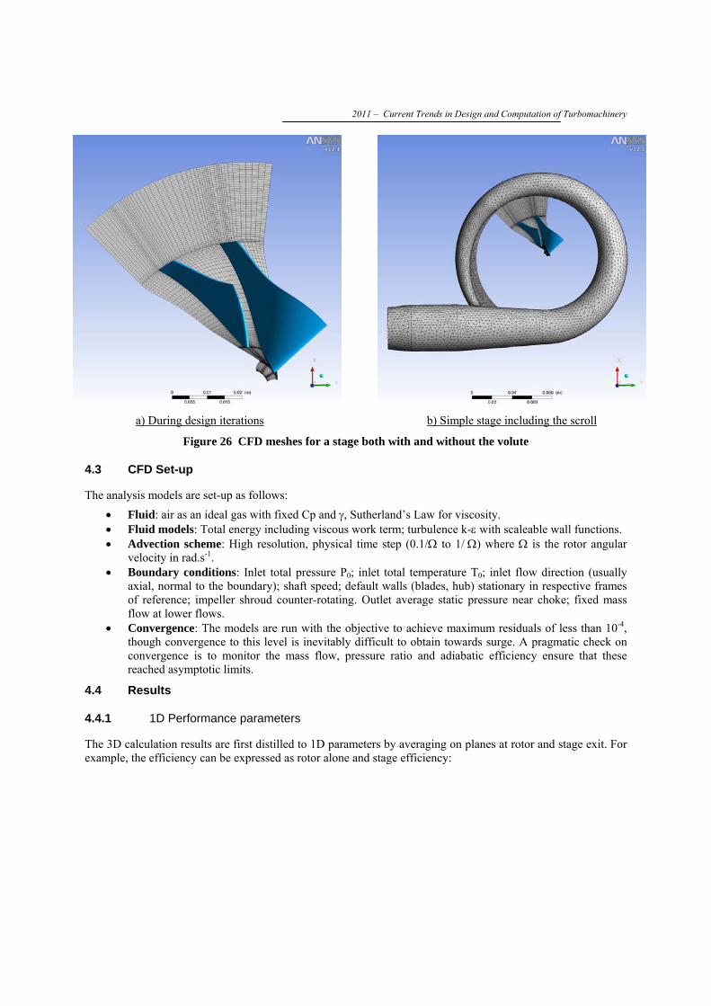
Normally in the design iterations only one passage of an impeller (or main vane plus splitter) is analysed and a single diffuser passage. Full-360° is achievable with parallel processing on PC clusters, but not generally practicable for the throughput necessary to assess each design iteration at a number of operating points in a reasonably short elapsed time. The impeller and diffuser are meshed as separate blocks with structured meshes, examples are shown in fig 26. Structured grids are preferred for bladed components, unstructured meshes are possible but need an order of magnitude more nodes to achieve results of similar quality. For the impeller, including the part of the intake considered, the grid in fig 26 has 99x66x34 (4 cells in the clearance gap) in the meridional, blade-to-blade and spanwise directions respectively. The vaneless diffuser has 41x66x34, making 314,160 nodes in total. For vaneless diffusers, connection is possible with a frozen rotor interface, ie the impeller is analysed in the rotating frame of reference and the diffuser in the stationary frame. When vaned diffusers are used the connection between the impellers and diffuser uses a ‘stage’ general grid interface (ggi). At this level of mesh density, the results cannot be assumed to be completely mesh-independent so it is highly desirable that the meshes are very repeatable in terms of topology, node count and relative distribution.

For cases including the volute, that component uses and unstructured mesh with tetrahedral elements in general but with hexahedral inflation layers adjacent to the walls, typically 350,000 nodes were used. The simplest form of the full stage calculation couples the single passage rotor and diffuser grids to the volute using a ‘stage’ ggi, necessary because of the change in pitch. The stage exit performance is evaluated at the end of the diffusing cone. An extension is applied to the model downstream of that averaging plane (a constant area section followed by a slightly converging final nozzle, fig 26) to avoid potential convergence difficulties with any flow separation on the outlet boundary. Note that the rotor and diffuser grids are placed at an ‘average’ position relative to the scroll, not close to the outlet scroll and ‘tongue’.


a) During design iterations b) Simple stage including the scroll

Figure 26 CFD meshes for a stage both with and without the volute

4.3 CFD Set-up

The analysis models are set-up as follows: • Fluid: air as an ideal gas with fixed Cp and γ, Sutherland’s Law for viscosity. • Fluid models: Total energy including viscous work term; turbulence k-ε with scaleable wall functions. • Advection scheme: High resolution, physical time step (0.1/Ω to 1/ Ω) where Ω is the rotor angular

velocity in rad.s-1. • Boundary conditions: Inlet total pressure P0; inlet total temperature T0; inlet flow direction (usually

axial, normal to the boundary); shaft speed; default walls (blades, hub) stationary in respective frames of reference; impeller shroud counter-rotating. Outlet average static pressure near choke; fixed mass flow at lower flows.

• Convergence: The models are run with the objective to achieve maximum residuals of less than 10-4, though convergence to this level is inevitably difficult to obtain towards surge. A pragmatic check on convergence is to monitor the mass flow, pressure ratio and adiabatic efficiency ensure that these reached asymptotic limits.

4.4 Results

4.4.1 1D Performance parameters

The 3D calculation results are first distilled to 1D parameters by averaging on planes at rotor and stage exit. For example, the efficiency can be expressed as rotor alone and stage efficiency:


1

1

01

05

1

01

021

−⎟⎟⎠

⎞⎜⎜⎝

⎛

−⎟⎟⎠

⎞⎜⎜⎝

⎛

=

−

TT

PP

R

γγ

η

1

1

01

05

1

01

05

−⎟⎟⎠

⎞⎜⎜⎝

⎛

−⎟⎟⎠

⎞⎜⎜⎝

⎛

=

−

TT

PP

stg

γγ

η

In this way the efficiency is broken down to three values: impeller just inside the trailing edge; impeller after mixing of wakes; overall stage, ie accounting for the diffuser loss. The total-static performance can also be quoted, this accounts no recovery in the outlet scroll and diffuser, the most pessimistic assumption. Planes 2.1 and 3 are either side of the mixing plane, 5 is at diffuser outlet.

Similarly, the diffuser loss coefficient and static pressure recovery can be calculated:

303

05030

pPPP

DP

−−

=Δ

303

35

pPppCp

−−

=

Note that there is no accounting of the volute performance in these predictions. Area-averaging is generally used at PCA, though use of mass-averaging could be supported for parameters including a dynamic component such as total pressure or temperature. Area-averaging tends to give results that are more conservative.

VIGV (40°) impeller and VVD (12°) Measured characteristics at Mu2 = 0.84

Figure 27 CFD model and test data for a stage with variable inlet guide vane and variable diffuser

Fig 27 shows a single stage air compressor comprising of a variable inlet guide vane (VIGV) a fixed speed impeller and a variable stagger diffuser vane (VVD). Test data is also shown, it is important that the stage can deliver a constant pressure rise down to a ‘turndown’ flow of 40% of design flow with minimal loss in efficiency. Fig 28 shows results of CFD analysis on a similar stage, but with a fixed diffuser vane at a tip Mach number Mu2 of 0.98.


0.2

0.3

0.4

0.5

0.6

0.7

0.8

0.9

1.0

0.04 0.09 0.14 0.19 0.24

Flow Coefficient (MGB)

DP/rU^2DH/U^2eta

Figure 28 Dimensionless stage performance over range of IGV settings

Fig 28 shows the CFD-predicted performance with prescribed inlet whirl angles of, from left to right, -60°, -50°, -30°, 0°, +10°. The performance is presented in dimensionless form of efficiency (η) ΔH/U2 and ΔP0/ρU2 (=ηΔH/U2) against the flow coefficient (4/πφt1) which is 0.176 at the nominal condition. The curves show that the peak pressure coefficient falls at turndown when, ideally, it should remain constant. A guide vane setting of about 60° looks likely to be necessary to reach the turndown flow on the basis of fig 28.


0.0

0.1

0.2

0.3

0.4

0.5

0.6

0.7

0.8

0.9

1.0

0.04 0.09 0.14 0.19 0.24

Flow Coefficient (MGB)

-90

-80

-70

-60

-50

-40

-30

-20

-10

0

10

eta2.1eta6.0DP/D2.1-5Mn3Cp2.1-5.0alpha3.0alpha5.0

Figure 29 Performance parameters over range of IGV settings

Fig 29 expands on the data in fig 28 to give a more detailed breakdown of the performance of the two components, impeller and diffuser. The data relates to the same 5 curves as given in fig 28 and these are discernible in fig 29. The predicted impeller efficiency increases slightly as the flow is reduced, presumably benefiting from reducing levels of inlet Mach number.

The diffuser is subjected to increasing inlet absolute gas angle as the flow is reduced though there is some flattening at the lowest flow coefficients when the angle is above 70°. The absolute Mach number remains constant initially but then rises below a flow coefficient of 0.14, exacerbating the problem for the diffuser associated with the incidence increase. The diffuser performance is characterised by the static pressure rise coefficient (Cp) and its loss coefficient (ΔP0/D). The minimum loss is centred on the nominal flow coefficient and shows a region where loss is reasonably constant between flow coefficients of 0.15 and 0.20 where the inlet angle varies between 65° and 51°.

As flow reduces below 0.15, the loss increases steadily. Also, the bladerow reaches its maximum Cp at the flow coefficient of 0.15 and the diffuser is stalling at lower flows. At flows above 0.21, the loss rises rather more sharply than it did on the low flow side of the minimum and Cp falls steeply. The outlet angle from the diffuser, evaluated at plane 5.0, is also shown in fig 29. Whilst the vane is operating around the bottom of its loss loop, the exit angle is almost constant.


After the point at which the pressure recovery changes slope (flow coefficient of 0.15) there is rather more ‘noise’ in the predicted exit angle though there is a peak-to-peak variation of only ±5° across the whole flow range.

Three typical IGV settings are considered below, fully open (0°) 40° and 61°; fig 30 illustrates the calculation domain and mid-span results.

0° Setting 40° Setting 61° Setting

Figure 30 CFD on an inlet guide vane

Despite its simple profile (a flat plate with bevelled edges) the vane does a good job at deflecting the gas. There is a separation zone at both 40° and 61° settings in fig 30 along much of the suction surface of the vane, but the flow is quite stable, assisted by the generally accelerating flow. A development could be to consider a profiled vane where the separated zone would be ‘filled’ by metal, it would be similar to the VVD in cross-section. However, it is doubtful that this would have a major impact on performance; the dynamic head in this region is quite low due to the high cross-sectional area so the absolute loss in total pressure is small.

The trends are generally to apply more complex CFD in an analysis mode, if not part of the iterative design procedure. Fig 31 shows the model for one stage from a multistage analysis including a complex 3D radial flow inlet, impellers, vaneless diffusers, vaned return channels and all leakage and seal flows, both along the shrouded impeller covers and up the backface of each impeller.


Figure 31 CFD model for an industrial stage, part of a multistage analysis

Fig 32 shows a similar case but two-stages with vaned diffusers, return channel and scroll. The leakage from the outlet of the return channel through to the tip of the upstream impeller is illustrated, coloured by temperature. For stages of significant Mach number is becomes important to be able to estimate this leakage flow and to account for it in sizing the diffuser.

Figure 32 CFD model for a two-stage compressor with open wheels and leakage flows

While fig 32 shows a case where only single passages of the vaned components have been modelled, with connections generally through stage ggi’s, fig 33 shows a full-360° model of a turbocharger compressor stage.


1

2

3

4

5

6

0.0 0.1 0.2 0.3 0.4 0.5Mass flow (kg/s)

Pressure ratio

0.300.350.40

0.450.500.550.600.650.700.750.800.85

Efficiency

Figure 33 Full-360 model and CFD results for a turbocharger compressor stage, vaneless diffuser

The full-360° model (green) was run at tip-speeds of 380m/s, 460m/s and 540m/s; a simpler case with one passage for the impeller and diffuser was run at 440m/s, 460m/s and 520m/s and the results are shown in blue. There is very good agreement justifying the use of the simpler approach during the development of the design. There is potential for this to break down at well off-design conditions, for example just as stall is approached where the non-uniformity in flow associated with the tongue may have a relatively large impact.

4.5 Validation

Validation of CFD can be considered at many levels. Fig 34 shows a specific validation example based on a Moody chart where CFX with k-ε was found to give very good agreement with the hydraulically smooth curve (and with laminar flow). This is very encouraging but not specific to the flow with turbomachinery.


Figure 34 CFD validation against the Moody chart

Fig 35 shows a comparison between area-averaged CFX results for a compressor stage in air with impeller and vaned diffuser at tip Mn levels of 1.2, 1.4 and 1.5. This again shows very good agreement, though the comparison is far more difficult to achieve due to issues relating to how parameters are measured on the one hand, and how well the CFD model is able to reproduce the geometry on the other.

1

2

3

4

5

6

7

4.0 4.5 5.0 5.5 6.0 6.5 7.0 7.5 8.0

Flow

Pres

sure

ratio

0.3

0.4

0.5

0.6

0.7

0.8

0.9

Δ

H/U

2 an

d ef

ficie

ncy

Figure 35 CFD validation on a high Mach number compressor stage with vaned diffuser

Validation on internal flow details is extremely rare within the compressor stages. An example of a diffuser from a compressor at impeller tip Mach number of 1.4 shown in fig 36. The flow visualisation from the test component was as a result of dirt becoming trapped in oil. The CFD result captures very well the point of separation using a mesh set-up as described above and the k-ε turbulence model.


Figure 36 CFD validation on the internal flow in a vaned diffuser

Another piece of validation data from a high Mach number compressor test (1.5) is shown in fig 37, the casing static pressure distribution over the impeller. The impeller leading edge is at z = 0 and he splitter at z = 50mm. The measured data is time-averaged as the vanes pass the measurement locations, the CFD results are pitchwise-averaged but the agreement is very encouraging.

-0.2

0.0

0.2

0.4

0.6

0.8

1.0

-60 -40 -20 0 20 40 60 80 100 120

z (mm)

Nor

mal

ised

sta

tic p

ress

ure

CFXTest

Figure 37 CFD validation on impeller shroud static pressure distribution


5. MECHANICAL ANALYSIS

The application of FE to turbomachinery components is in a well-developed state, at least when considering typical design iterations which are normally considered to be linear and elastic. The calculation of key parameters such as maximum stresses in the vanes and discs and natural frequencies are used to establish that the components have adequate safety margins operating at their steady stresses and that there is no possibility to excite the natural frequencies. It will normally be necessary to pass through these conditions as the machine operates transiently but prolonged excitation could result in a fatigue failure.

Given that FE is reliable and well established, the main challenge is to make the solutions available in a seamless and timely manner, particularly for those cases that are more likely to be critical in terms of excitation of natural frequencies, such as high specific flow centrifugal compressors.

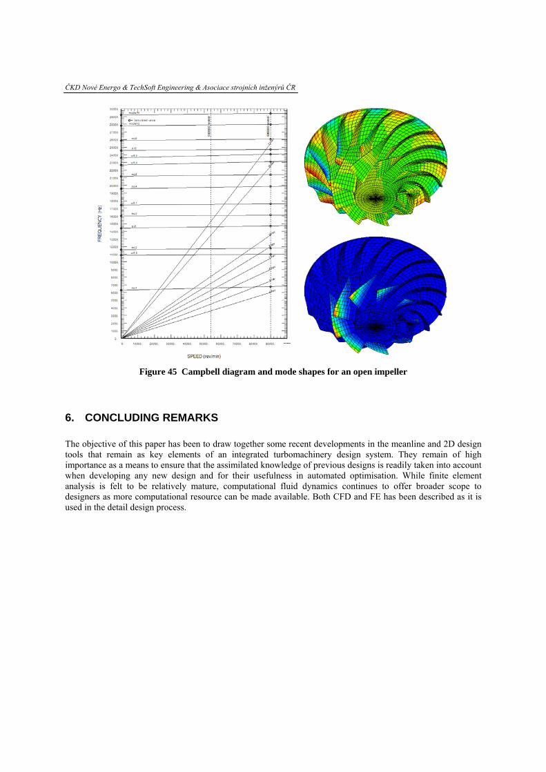
During the early aerodynamic design iterations it is good practice to assess the first flap frequency of the main vane as the vane geometry is developed aerodynamically, particularly for open wheels with relatively high specific flow. The stiffness of the vane is affected by the thickness ‘taper ratio’, ie the thickness at the hub of the vane compared with the shroud, the meridional distribution of vane camber and thickness, the slope of the hub in the meridional direction. These parameters are highly coupled and it is only practicable to assess the frequency by analysis rather than ‘rule of thumb’. This can be easily done with a main-vane-only 3D FE analysis, ie with the vane fully constrained at the hub. This results in frequencies that are slightly higher than would be achieved using a full 3D model including the disc, which adds flexibility, but the over-prediction has been found to be consistent (+5%) so the results can be calibrated for a particular class of impeller. Fig 38 compares results from vane-only with full 3D for a high specific flow turbocharger impeller. The analysis takes only a few seconds and is therefore usefully incorporated into PCA’s BGA optimisation procedure.

Vane only 3D – 1F = 10,245Hz Full 3D – 1F =9688Hz

Figure 38 Predicted first flap frequencies for the main vane of an open impeller


A full 3D elastic finite element analysis is carried out towards the end of the design cycle, it may be necessary to include the effects of temperature variation in the analysis, but pressure loads are often negligible when compared to the stresses due to rotation. Also a modal analysis will be carried out, usually with the impeller at rest and at design speed including the effects of stress-stiffening.

Material properties can be a difficult issue, their acquisition is expensive and time-consuming and these data are highly sensitive and proprietary where they have been gathered for internal use by a manufacturer. Useful data can be found in the public domain, for example MIL-HDBK-5F. For 17.4PH steel forging typical values at 350°C are: Density, ρ : 7800 kg/m3 Poisson’s ratio, ν : 0.3 Yield stress, σy : 675 MPa Tensile strength, σu : 817 MPa Young’s modulus, E : 0.1763x106 MPa From these the following criteria could be chosen: Design stress, direct : 0.67 x σy = 452 MPa Design stress, bending : σy = 675 MPa A considerable body of experimental data has shown that the speed at which a disc will burst tangentially depends almost entirely on the area weighted mean hoop stress, θσ or the volume weighted mean equivalent

stress eqσ . As the wheel over-speeds beyond the point where the maximum stressed region begins to yield, the increased centrifugal load will, primarily be absorbed by the remaining elastic regions of the disc. As the speed is increased further the proportion of the wheel remaining elastic reduces until the ultimate tensile strength of the material has been reached at all points of the cross section. A further increase in speed theoretically results in complete fracture. This is what happens with an ideally ductile and non-notch sensitive material. However, actual discs burst when the stress attains a value of between 75% and 100% of the ultimate tensile strength. The burst margin is defined as the ratio to the design speed at which θσ or eqσ becomes equal to some safety factor, F times the ultimate tensile strength of the material. The safety factor, F, is usually taken to be between 0.7 and 0.75 and an acceptable burst margin should be >1.4.

θσ

FxUTSNN

d

b =

where is the burst speed bN is the design speed dNThe area weighted mean hoop stress may be computed from the results of a finite element axi-symmetric stress analysis in the following manner:

∑∫=

=

=ni

id

dAA 1

1θθ σσ


where = cross sectional area of the disc dA n = number of elements constituting the disc Similarly the volume weighted mean equivalent stress is computed in the following manner from the results of a 3D finite element stress analysis.

∑∫=

=

=ni

ieq

deq dV

V 1

1 σσ

where = volume of the disc dV = number of element constituting the disc nThe disc shape is normally developed using 2D FE, as in fig 39.

Figure 39 Influence of backface extension on 2D von Mises stresses

Purely radial discs are used where axial length is at a premium. However, the tendency is for the rim to lean forwards when the impeller runs and the tendency to do this can be offset by making the disc more symmetric using a backface extension. Applying a backface extension of order 6% of the vane dip diameter reduces the bore stress by about 30% and the forward displacement by a similar amount. Control of the forward displacement is useful in the case of open wheels, the build clearance can be reduced so the part-speed clearance is also reduced.

A two dimensional axisymmetric stress analysis was conducted for the disc with and without the shroud at 387m/s. The vanes were modelled as plane stress elements with a nodal thickness distribution corresponding to the vane geometry. The von-Mises stress distribution for these two cases are illustrated in fig 40.


Open impeller Shrouded impeller

Figure 40 Von-mises stresses, axisymmetric models

For the disc with no shroud the maximum stress occurs at the bore with a value of 382 MPa. The area weighted mean hoop stress was computed to be 150.3 MPa. For the disc with shroud added the maximum stress again occurs at the bore with a value of 406 MPa and a computed area weighted mean hoop stress of 171.7 MPa.

The shroud always exerts a tensile load on the vanes. The shroud thickness must, therefore, be minimized consistent with maintaining acceptable bending stresses which, will occur in the circumferential direction. The dominating factor influencing the stresses in the vane and shroud is the ratio of the vane thickness at the shroud to the thickness at the hub. This effect may be seen with reference to fig 41 where the vane thickness at the shroud can be seen to have a significant effect on the maximum stress in the vane. Using a constant vane thickness reduces the stress by a factor of approximately 2.

a) Vane thickness ratio = 0.375 b) Vane thickness ratio = 1.0

Figure 41 Effect of vane taper ratio on vane stress with a shrouded impeller


The rake of the vane at the trailing edge also influences the stress in the vanes. Fig 42illustrates rakes of 25° and 45° which spans the normal range used at PCA. Typically the application of 45° of rake reduces the stress in the vane surfaces by 20-40% compared with zero rake, ie the vane normal to the backface at impeller exit. It is a complex issue, however, depending on the relative stiffness of the vanes and backface and can only be optimised on a case-by-case basis with 3D FE analysis.

a) Rake of 25° b) Rake of 45°

Figure 42 Vane exit rake in open impellers

A typical 3D FE mesh is illustrated in fig 43. The mesh comprises 20-noded brick elements with mid-side nodes. Analysis is performed using complex constraints so that the vibration results for disc modes at all nodal diameters can be obtained from the single-segment model which greatly reduces analysis computational effort.

Figure 43 Segmental finite element model, shrouded impeller


The von-Mises stress distributions in the impeller at a tip-speed of 417m/s are illustrated in fig 44. The maximum bore stress is 500MPa and the computed area weighted mean hoop stress is 220MPa. The maximum stress occurs at the vane trailing edge with a value of 650MPa.

Figure 44 von Mises stress distributions in a shrouded impeller

The same model is used for modal analysis and the results expressed in the form of a Campbell diagram, fig 45 along with two mode shapes, 1 and 10. Mode 1 is ‘first-flap’, 1F, and involves movement of only the vanes; mode 10 is a higher order complex shape involving movement of the vane and disc. The normal design criteria is for 1F to be above potential excitation at 4 per rev. This avoids harmonics of out of balance forces and is believed to be a conservative approach.

Other ‘spokes’ plotted on the Campbell diagram will include, for example, those related to any struts in the intake, or inlet guide vanes ahead of the impeller and the vaned diffuser, if present. Although the higher order modes are generally less accurately predicted than the lower modes (which are typically accurate to about 2%) it remains good practice to aim to avoid possibility of excitation.


Figure 45 Campbell diagram and mode shapes for an open impeller

6. CONCLUDING REMARKS

The objective of this paper has been to draw together some recent developments in the meanline and 2D design tools that remain as key elements of an integrated turbomachinery design system. They remain of high importance as a means to ensure that the assimilated knowledge of previous designs is readily taken into account when developing any new design and for their usefulness in automated optimisation. While finite element analysis is felt to be relatively mature, computational fluid dynamics continues to offer broader scope to designers as more computational resource can be made available. Both CFD and FE has been described as it is used in the detail design process.


7. REFERENCES

1. Casey, M.V., (1983) "A computational geometry for the blades and internal flow channels of centrifugal compressors", ASME Journal of Engineering for Power, Vol.105, April 1983, pp 288-295.

2. Casey, M.V.,(1994) "Computational Methods for Preliminary Design and Geometry Definition in Turbomachinery", AGARD-LS-195, AGARD Lecture Series on Turbomachinery Design using CFD, NASA-Lewis, 1994.

3. Casey, M. V., and Fesich, M., (2010), “The efficiency of turbocharger components with diabatic flows”, ASME Journal of Engineering for Gas Turbines and Power, July 2010, Volume 132, Issue 7.

4. Casey, M.V., Gersbach, F., Robinson, C.J, “A new optimisation technique for radial compressor impellers”, ASME TURBOEXPO 2008, Berlin, ASME GT2008-50561

5. Casey, M.V., and Marty, F., (1985) "Centrifugal compressors - performance at design and off-design", Proceedings of the Institute of Refrigeration, London, Volume 1985-86.

6. Casey M. V., Robinson C. J. (2006) “A guide to turbocharger compressor characteristics”, published in “Dieselmotorentechnik”, 10th Symposium, 30-31 March, 2006, Ostfildern, Ed. M. Bargende, , TAE Esslingen, ISBN 3-924813-65-5

7. Casey, M.V., and Robinson, C.J., (2010), “A new streamline curvature throughflow code for radial turbomachinery”, ASME Journal of turbomachinery, 2010, vol. 132, April.

8. Casey, M.V and Robinson, C.J. (2011) “ A unified correction method for Reynolds number, size and roughness effects on the performance of compressors”, 9th European conference on Turbomachinery , 21-25 March 2011, Istanbul Turkey, to be published in the Journal of power and Energy.

9. Casey, M.V., and Roth, P., "A streamline curvature throughflow method for radial turbocompressors", I.Mech.E. Conference on Computational Methods in Turbomachinery, Birmingham, April 1984.

10. Cumpsty, N. A., (1989), Compressor Aerodynamics, Longman Group Ltd., Pearson Education Ltd, Harlow, Essex, U.K.

11. Rodgers, C. (1964), “Typical performance characteristics of gas turbine radial compressors”, Trans ASME, Journal of Engineering for Power, Vol. 86.

12. Rodgers, C., (1980) “Efficiency of centrifugal compressor impellers”, Paper 22 of AGARD conference proceedings No 282 Centrifugal Compressors, Flow Phenomena and Performance, Brussels May 1982.

13. Rodgers, C., 1992, “Centrifugal compressor design: state of the art performance”, Cranfield University short course on centrifugal compressors, March, Cranfield University.

14. Simon H., and Bülskämper A., (1984), “On the Evaluation of Reynolds Number and Relative Surface Roughness Effects on Centrifugal Compressor Performance Based on Systematic Experimental Investigations”, ASME, Journal of Engineering for Power, April 1984, Vol. 106, pages 489-501.

15. Stanitz, J.D and Prian V.D. (1951) “A rapid approximate method for determining velocity distribution on impeller blades of centrifugal compressors”, NACA TN 2421.

16. Swain, E., (1990), “A simple method for predicting centrifugal compressor performance characteristics”, Proceedings of IMechE Conference, C405/040, 1990.

17. Wiesner, F. J., (1967), “A review of Slip Factors for Centrifugal Impellers”, Trans. ASME Jnl Eng. Power, Vol 89: pages 558-72, 1967.

Date post:	18-Jun-2018
Category:	Documents
Upload:	hanhi
View:	215 times
Download:	0 times

An integrated approach to the aero-mechanical optimisation … · ABSTRACT: The design of...

Documents