An Integrated Bioinformatics Pipeline for Single Cell RNA-seq Analysis Application in Natural Killer Cell Differentiation Herman K. Netskar Thesis submitted for the degree of Master in Informatics: Technical and Scientific Applications (Imaging and Biomedical Computing) 60 credits Department of Informatics Faculty of Mathematics and Natural Sciences UNIVERSITY OF OSLO Spring 2019
Transcript
An Integrated BioinformaticsPipeline for Single Cell RNA-seq
Analysis
Application in Natural Killer Cell Differentiation
Herman K. Netskar
Thesis submitted for the degree ofMaster in Informatics: Technical and Scientific
Applications (Imaging and Biomedical Computing)60 credits
Department of InformaticsFaculty of Mathematics and Natural Sciences
UNIVERSITY OF OSLO
Spring 2019
An Integrated BioinformaticsPipeline for Single Cell
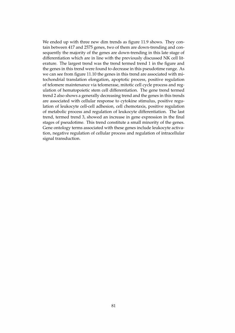
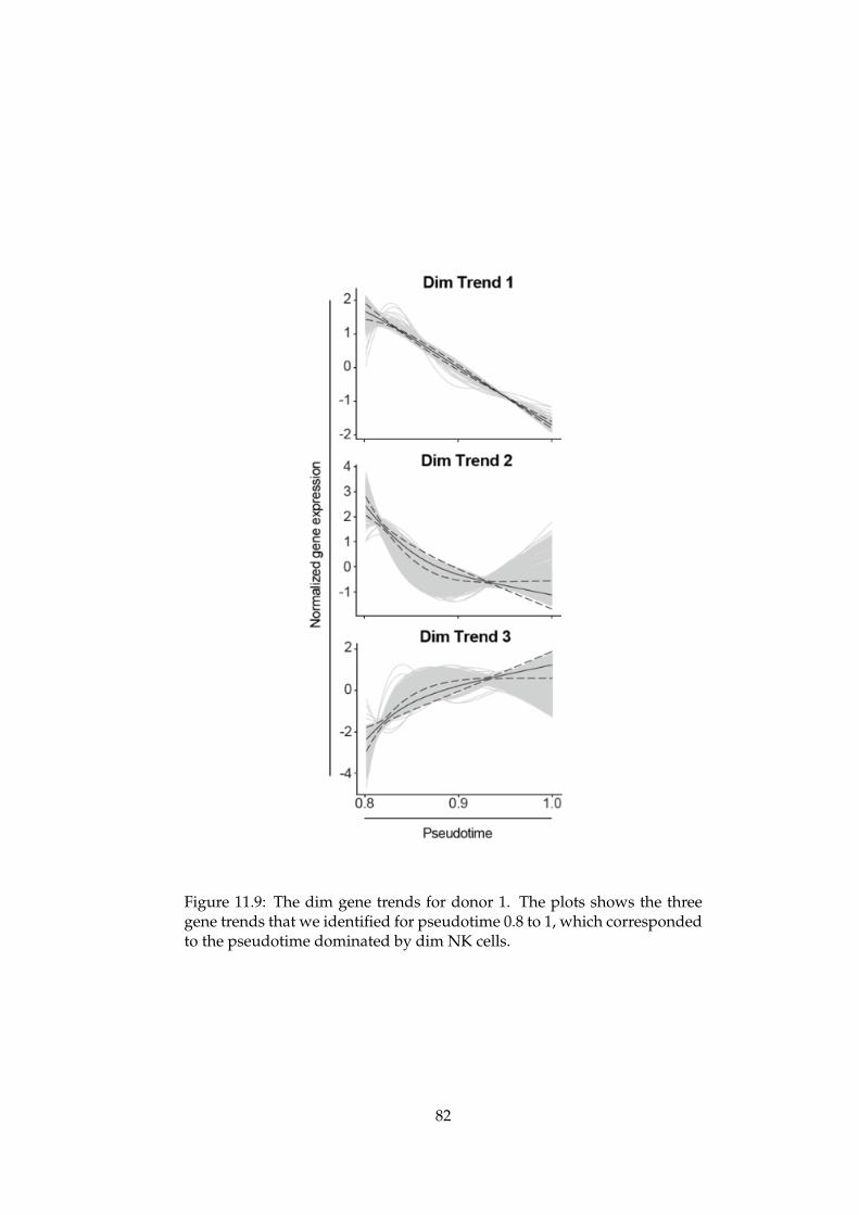
Single cell RNA-sequencing is an increasingly popular tool for investigat-ing the variability in gene expression between individual cells. Comparedto the previously wide spread methods such as bulk RNA-sequencing, thesingle cell approach gives the advantage of a much higher cellular resolu-tion, but it also provides us with much noisier data. In the recent yearsa large number of bioinformatics tools have been developed to analyzescRNA-seq data. There is an abundance of methods, for example morethan 50 methods for trajectory inference have been developed since 2014[1]. Many of the tools previously developed for bulk RNA-seq can also beapplied to single cell data, but there are some crucial differences in the in-herent characteristics of the data that differentiates scRNA-seq data fromits bulk counterpart, among others in the statistical characteristics of thedata [2].
In order to use the large amounts of data generated by scRNA-seq toproduce new biological insights, we need to integrate the relevant toolsinto an integrated coherent framework. This thesis presents a pipelinethat I developed, called SingleFlow, to perform large scale analysis insuch an integrated framework. The pipeline’s usefulness was validatedby applying it in the context of natural killer (NK) cell biology. Thereare a number of questions unanswered in the field of NK cell biology. Byapplying the pipeline to a unique scRNA-seq data set of NK cells from twodifferent donors, we identified a temporal transcriptional map of humanNK cell differentiation.
By mapping gene expression trends to pseudotime, we identifieddistinct transcriptional checkpoints that represent changes during NK celldifferentiation. We also identified previously undescribed subsets withinthe CD56bright subset of NK cells. The combination of the pipeline’sanalysis and the potential of the novel data set proved useful in identifyingimportant gene programs that are associated with NK cell differentiation.This knowledge holds potential to guide the development of new strategiesfor NK cell-based cancer immunotherapy.
2.3.1 NK cell differentiation and education . . . . . . . . . 82.3.2 Unknown factors in NK cell differentiation . . . . . . 92.3.3 Use of NK cells in cell therapies for cancer . . . . . . 10
2.4 Single cell RNA sequencing . . . . . . . . . . . . . . . . . . . 102.4.1 How scRNA-seq data is generated . . . . . . . . . . . 112.4.2 Challenges working with scRNA-seq data . . . . . . 112.4.3 The need for bioinformatics . . . . . . . . . . . . . . . 12
9.3 A comparison of SingleFlow to other scRNA-seq pipeline tools 579.4 User guide . . . . . . . . . . . . . . . . . . . . . . . . . . . . . 59
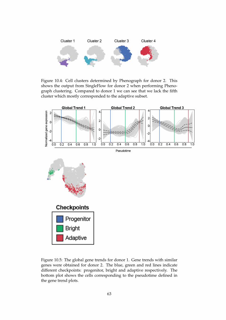
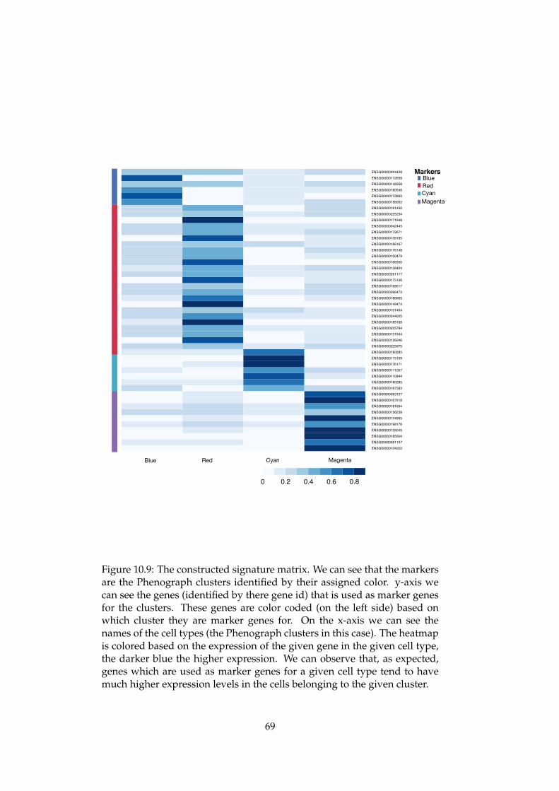
10 Validation 6110.1 Reproduce results across donors . . . . . . . . . . . . . . . . 6110.2 Reproducing results from NK cell differentiation literature . 6510.3 Recover the cell type composition in RNA-seq data using
11 User scenarios: applications in single cell NK cell biology 7111.1 NK cell differentiation defined through single cell RNA-seq 7111.2 Continuous and coordinated transcriptional changes in
7.1 The subset sorting done prior to scRNA-seq . . . . . . . . . . 437.2 Pipeline to generate count data using Cell Ranger . . . . . . 44
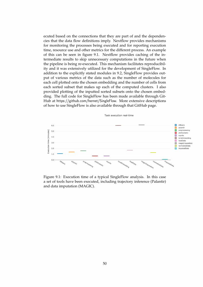
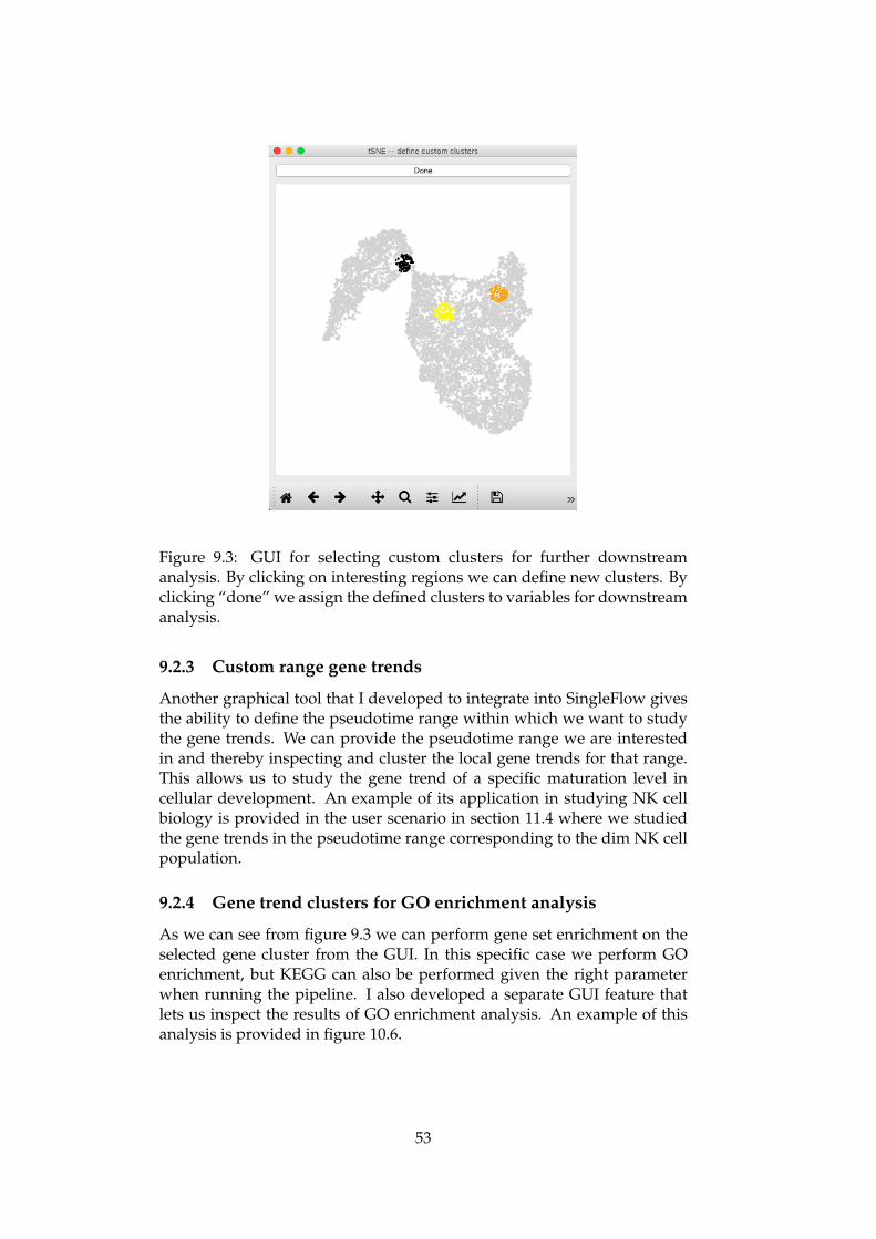
9.1 Execution time of a typical SingleFlow analysis . . . . . . . . 509.2 Outline of the processes in SingleFlow . . . . . . . . . . . . . 519.3 GUI for selecting custom clusters for further downstream
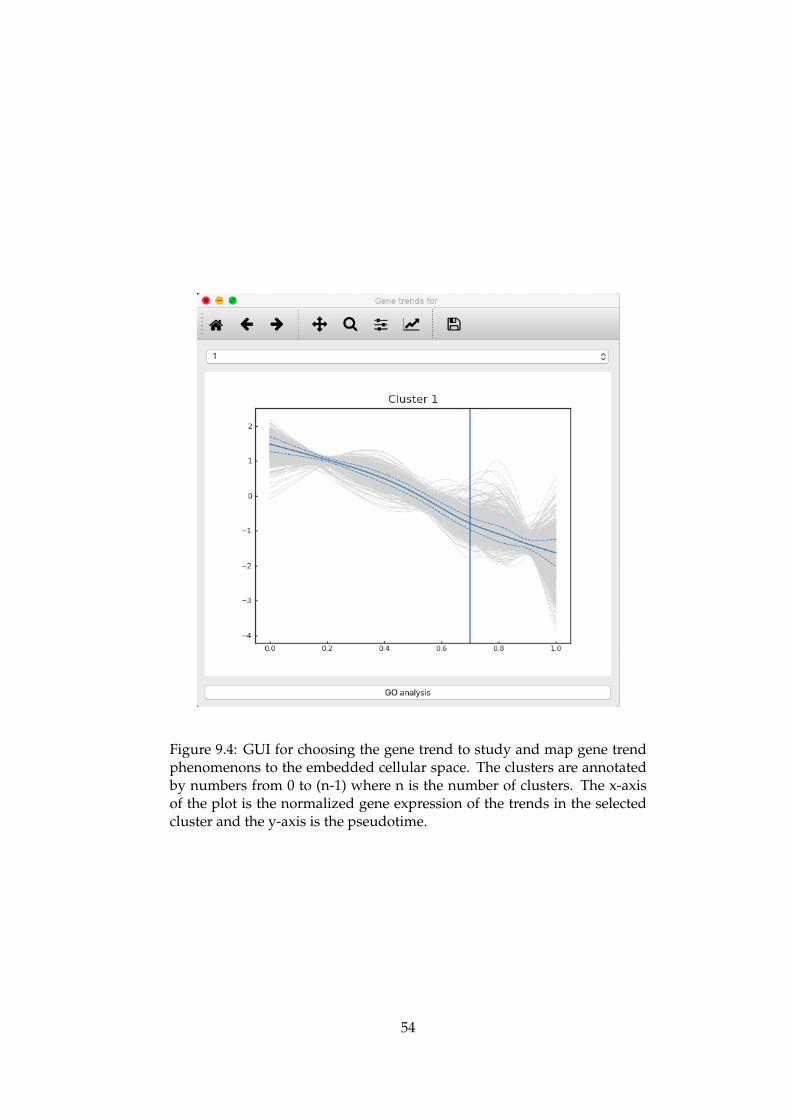
analysis. . . . . . . . . . . . . . . . . . . . . . . . . . . . . . . 539.4 GUI for choosing the gene trend to study and map gene
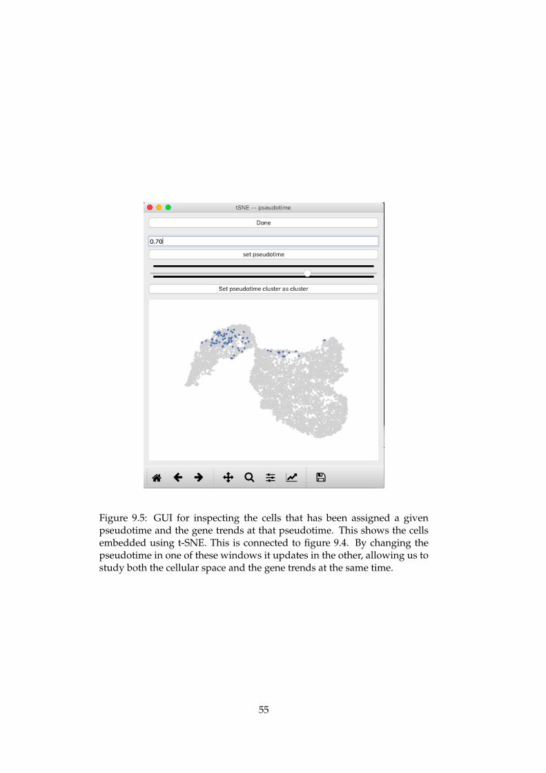
trend phenomenons to the embedded cellular space . . . . . 549.5 GUI for inspecting the cells that has been assigned a given
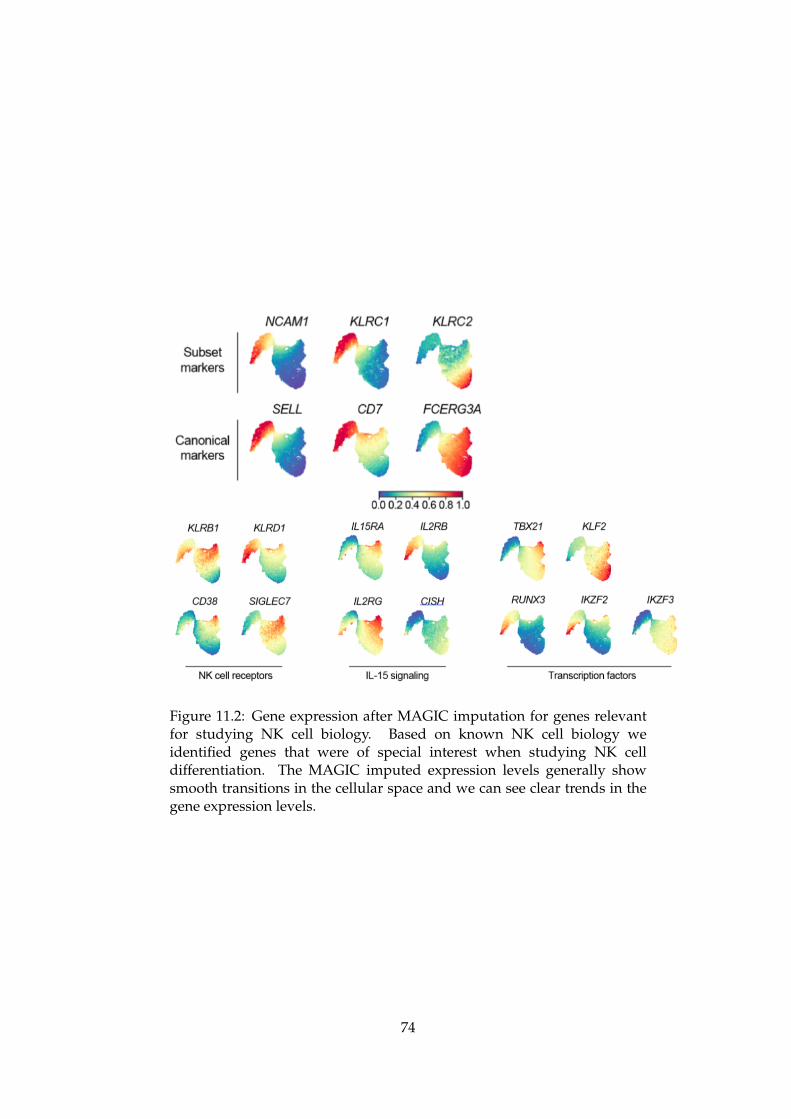
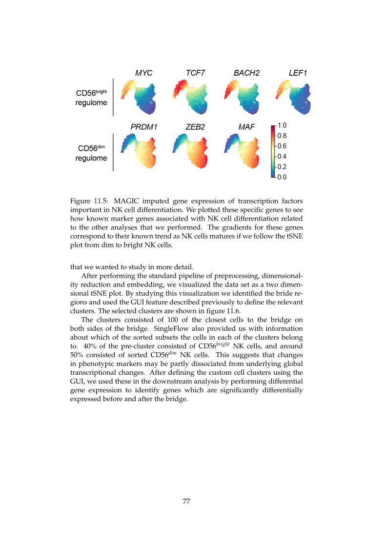
11.3 The composition of the different clusters . . . . . . . . . . . . 7511.4 RNA velocity embedded in the t-SNE plot . . . . . . . . . . . 7611.5 MAGIC imputed gene expression of transcription factors
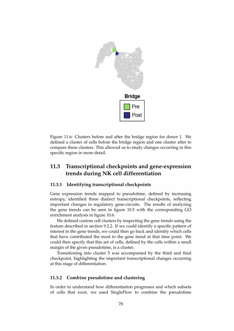
important in NK cell differentiation. . . . . . . . . . . . . . . 7711.6 Clusters before and after the bridge region for donor 1 . . . 7811.7 Pseudotime plotted onto the t-SNE embedding . . . . . . . . 7911.8 Boxplot combining the pseudotime computation with the
Before I started working on this project I had no experience working inthe field of single cell RNA-sequencing. My background was mostly ininformatics generally, with some statistics courses and a couple of yearsof studying medicine as a good complement. I had also taken a course inbioinformatics, and found the idea of combining the study of biological andmedical phenomenons with the quantitative nature of computer science,appealing.
I learned a lot from working on this project. Both about the field ofscRNA-seq and NK cell biology specifically, but also about the scientificprocess generally. Especially working towards writing a paper was a veryrewarding experience. The interdisciplinary nature of bioinformatics madeit even more fulfilling.
First and foremost I would like to thank my main supervisor TrevorClancy for his help and guidance throughout my work on this project. Iwould also like to thank my co-supervisor Eivind Hovig. Working in theinterdisciplinary field that bioinformatics is, the project called for collabor-ations. Throughout this project I have collaborated with biologists from theMalmberg Lab at the Oslo University Hospital. I would specifically like tothank Professor Karl-Johan Malmberg and Aline Pfefferle for the collabor-ation and the valuable biological insight they provided.
Herman K. NetskarOslo, May 2019
xi
xii
Part I
Introduction
1
Chapter 1
Introduction
1.1 Motivation
Natural killer (NK) cells are central cells of our innate immune systemthat can lyse tumor cells. NK-cell-based immunotherapeutic strategieshave recently been developed to target human cancers [3]. The successfulapplication of this type of therapy requires an in depth understandingof NK cells, their biology and their development. The regulatory geneprograms that define NK cell states and their differentiation dynamics arenot fully understood and an improved description of the programs thatcontrol clinically beneficial NK cell subtypes would be of great value forfuture immunotherapeutic strategies.
Recent advances in scRNA-seq analysis has provided new insightsin a variety of fields within molecular biology [4][5][6]. scRNA-seqcan potentially revolutionize the way we characterize immune cellsand their dynamics [7]. Utilizing new sequencing technologies andnewly developed analysis tools for scRNA-seq data could potentiallydramatically improve our understanding of NK cells, its regulatorymechanisms and differentiation in particular.
There is an abundance of tools available for scRNA-seq data analysis.Standalone tools and integrated toolkits already exist [8], but to gain ad-vanced biological insights the field needs a comprehensive and reprodu-cible analysis of single cell data. It would be useful to develop a frameworkand a pipeline to perform such an analysis. With the rapid development inthis field in mind, such a pipeline must also be developed in a way so thatnew tools easily can be included in the framework in order to complementand extend the analyses in the future.
The goal of using NK cells in immunotherapy and the potential ofscRNA-seq data analysis to retrieve the necessary biological insight tomove towards this goal, was the main motivation behind this project.
1.2 Objectives
The main objective of this project was to develop an integrated andmodular pipeline for studying scRNA-seq data by integrating existing tools
3
as well as to develop new components where I found it necessary.Specifically I wanted to achieve the following:
• An improved modularization of scRNA-seq workflows: One of themain aims of this project was to establish a bioinformatics frameworkthat uses existing tools and integrate them so that different toolseasily can be switched out for newly developed tools (modularity). Iwanted the pipeline to be able to save the intermediate states, so thatanalysis can be run with different tools with the same input, as well asto facilitate automation and reproducibility of advanced scRNA-seqanalysis.
• Apply the framework to data sets of NK cells from the MalmbergLab, Oslo University Hospital, and verify that the analysis providedby the pipeline offered biological insights in collaboration with NKcell biologists. By applying the developed pipeline to a novel NKcell data set, we wanted to try to answer some of the unansweredquestions about NK cell differentiation and NK cell subsets outlinedin the background chapter on NK cell biology.
1.3 About the thesis
This thesis consists of four main parts. Part I is an introduction to the fieldof single cell RNA-sequencing and some of the biology underpinning thisfield. In this part I discuss a little about cell fate and differentiation and whywe want to study this, specifically I talk about NK cells and their biology.In this part I also describe existing tools for processing scRNA-seq data andbioinformatics tools for analyzing this data. Part II discusses the methodsused as part of the project. It introduces the data sets that the pipelinewas applied to and describes how these data sets were generated. Itdescribes which tools I used and how these were integrated into a coherentframework for scRNA-seq data analysis. I also present justification forchoosing these specific tools.
Part III consists of the results from the project. SingleFlow, the pipelinethat I developed, is the main outcome of this project. However the projectwould not have been complete without the ability to gain some biologicalinsights from the final framework. I therefore present a set of user scenariosin the field of NK cell differentiation and describe the correspondingbiological interpretation of the results that SingleFlow produced. The finalpart, part IV, discusses these results and puts them into perspective. Itlooks at limitations of the analysis framework and looks at possible futurework. I also present some ideas of future applications of NK cells inimmunotherapeutic strategies and discuss why the analysis presented hereis useful in a broader perspective.
This project was carried out in collaboration with the Malmberg Lab atthe Oslo University Hospital. This research group studies the molecularand cellular basis of NK cell dynamics. By collaborating with biologistswho work in the field of NK cell biology I was able to assess the
4
tools I applied and gain insight into the biological questions that wouldbe relevant to try to answer using the scRNA-seq data sets and thesubsequent analysis. I have personally carried out the development ofthe SingleFlow framework and performed the analysis. Throughout thisthesis I will use the term ’I’ where I refer to work on SingleFlow and Iwill use ’we’ when discussing its application to NK cell biology and thecorresponding analysis and interpretation. The development of SingleFlowwas in large part motivated from discussions with the Malmberg Lab andthe subsequent collaboration. This collaboration helped me put the thebioinformatics analysis into an appropriate context. As a result of this wehave written a manuscript which is already submitted for publication.
5
6
Chapter 2
Background
2.1 Cell fate and differentiation
Immune cells develop over time by interactions with antigens and othercells, facilitated by controlled modifications in gene expression in the cellsas they develop [9]. Certain subsets of genes, known as gene regulatoryprograms, are important in regulating this dynamic process known ascell differentiation. In this process cells develop from one cell type toanother, often more restricted, cell type [10]. One goal in biology is tounderstand how cells develop, how they differentiate and how they endup in their final state. This is known as the cell’s fate, and biologistswant to understand the factors that determine it and which regulatory geneprograms that are relevant.
Differentiation has in the past been understood as a series of discretecell states, where there exist marker genes that are mutually exclusivebetween cells and therefore provides us with a clear classification of a givencell into one subset or another [11]. This has also been the main assumptionin the mathematical and statistical models that have underpinned the studyof cell fate [12]. However, recent developments [12] [13] have indicatedthat cell states make up a continuum and that the assumption of discretestates therefore is flawed. New sequencing technologies, and statistical andbioinformatics methods that will be discussed later, has been important inthis development.
2.2 RNA
RNA molecules are transcribed from a gene’s DNA template and some ofthe produced RNA molecules serve as templates for protein synthesis [14].The RNA molecules that provide genetic information for protein synthesisare known as messenger RNA (mRNA). The collection of all (protein-coding) mRNA in a cell is known as the cell’s transcriptome. Whethera gene is actively being transcribed and at what level this transcriptionoccurs tells us something about the cell’s state and each cell can inprincipal be placed in a number-of-genes dimensional space where eachfeature corresponds to a gene and the value for that feature is the level of
7
transcription for that gene. The value for an individual gene in a givencell can for example be the number of RNA molecules corresponding tothat specific gene in that cell. This means that a measurement of the wholetranscriptome of a cell effectively gives us a high dimensional vector torepresent that cell.
2.2.1 Splicing
For most human (and other eukaryotic) genes the initial RNA transcript(pre-mRNA) must be processed to become mature mRNA before proteinsynthesis can be carried out [14]. An important part of this processing issplicing, where certain parts of the RNA sequence is removed, or splicedout, in a multi-step process. After splicing we have the exon, which isthe sequence that goes on to become the mature mRNA, and the introns,which are the removed parts, separated. This means that when we doRNA sequencing of cells, the resulting data will contain transcripts whichare spliced and other transcripts which are unspliced. These transcriptscorrespond to the same genes even if the actual sequence of the transcriptsare different. The information of which genes whose corresponding mRNAmolecules are spliced and unspliced, in what proportion they are found inthese two forms, and in which cells these transcripts are found, can be usedin downstream analysis, for example in the computation of RNA velocity[15] which is one of the bioinformatics tools described and used later (seesection 4.3).
2.3 NK cell biology
Natural killer (NK) cells are lymphocytes (white blood cells) that sit onthe crossroad of innate immune response, which is the first step in theimmune defense, and the adaptive immune response, the specific part ofthe immune defense [16] [9] [17]. NK cells recognize and kill infected andstressed cells by secreting cytokines and chemokines [18] [9]. This secretionalso influence the adaptive immune response that follows. We can divideNK cells into two broad subsets based on their expression of the gene CD56,CD56bright and CD56dim. The bright subset is considered a set of less maturecells that can differentiate into dim NK cells. The dynamics of NK celldevelopment is however very complex and the number of differentiationpaths and subsets is very high [19].
2.3.1 NK cell differentiation and education
NK cells develop from common progenitors but diverge into distinctsubsets, which differ in cytokine production, cytotoxicity and other aspects[5]. An analysis in a 2013 paper revealed a large degree of NK cell diversity[19]. The authors of this paper estimated a total of more than 100,000 NKcell phenotypes.
There is a continuous differentiation of NK cells through a set ofintermediate states, from CD56bright NK cells to terminally differentiated,
8
so called adaptive NK cells. As CD56dim cells continue to differentiate theylose expression of the gene NKG2A and they acquire inhibitory killer cellinhibitory immunoglobulin-like receptors (KIR) and CD57. They also showa decline in the cells’ proliferation, which is the cells’ ability to increasein number [18]. The adaptive NK cells are called such because they havefunctions generally associated with the adaptive immune response. Thepresence of these adaptive cells is associated with past infection by a viruscalled cytomegalovirus [20] [21]. Physical interactions between cells leadto development of the NK cells’ functional potential [22]. The diversity ofNK cell phenotypes also stems from the process known as education.
NK cells have inhibitory receptors that suppress the cytotoxic activity ofthe cells. These receptors are specific for certain cell-surface proteins calledHLA, which are expressed on healthy human cells. These molecules tell theimmune system that the given cell is part of the “self”, i.e. that these cellsshould not be attacked by the immune system [9]. Without this inhibitorysystem, the NK cells would not only kill infected and otherwise unhealthycells, but would also be able to kill the healthy cells. There also exist othermechanisms for preventing NK cells from killing the healthy cells [23].The cells that express the inhibitory receptors that are capable of bindingto these HLA molecules get “educated” through a set of combinations ofreceptors and HLA molecules. The education of an NK cell by a specificHLA molecule is defined by whether it can sense if the given HLA moleculeis downregulated on a cell in order to activate its response against that cell[24].
The known marker genes and differentiation processes in NK cellbiology briefly outlined above can be incorporated into our analysis andbe used to verify the results of the scRNA-seq analysis to see if the analysiscan reproduce some of these. This is further discussed in section 8.1.
2.3.2 Unknown factors in NK cell differentiation
Several regulatory programs that define the differences between the brightand the dim NK cells are already established in the biological literature,but there are some major unknown factors in NK cell differentiation. Itis not clear how the bright and dim NK cell populations relate to otherphenotypically defined stages of NK cell differentiation. It is not knownwhether there exists intermediate cell states which can be described by theirtranscriptional signature even if they might be considered part of the sameNK cell subset when we only consider a few selected cell surface markergenes as we typically do when sorting cells before sequencing them (seesection 7.1). Another unknown factor in NK cell differentiation is whetherit is a linear process with distinct transcriptional checkpoints or not. Thesequestions will be studied and discussed later as I apply SingleFlow to anovel NK cell data set (see section 11).
9
2.3.3 Use of NK cells in cell therapies for cancer
There is evidence for NK-cell targeting of human tumors [3] and NK cellshave shown promise in so called adoptive cell therapies (ACT) [5]. ACTis a kind of cell therapy where phenotypically beneficial immune cells aretransferred into the patient with the goal of ending up with an improvedimmune response to the cancer [25]. The possibility of off-the-shelf celltherapy based on NK cells has also been described [26]. In order tofurther incorporate NK cells into therapeutic strategies, we would need toobtain a deeper understanding of regulatory modules controlling clinicallybeneficial NK phenotypes [5] [3]. As described previously (section 1.1) thisis one of the main motivations behind this project. The prospects of NK cellbased cell therapy and how this project fits into this context is discussed inmore detail in chapter 15.
2.4 Single cell RNA sequencing
Medical research increasingly deals with the cellular and molecular sideof biology [27], where the modification and understanding of cellularbehavior through targeted approaches are important. One way to measurea cell’s state is to look at the transcriptome of the cell as described insection 2.2. Single cell RNA sequencing (scRNA-seq) has recently becomea very popular method in biological research [28]. This method measurestranscriptome-wide gene expression in individual cells, in other words itcounts the number of different mRNA molecules found in each of the cellsin the sample being studied [29]. This provides us with a high dimensionalvector representing the transcriptional state of each cell as described insection 2.2.
Prior to the development of single cell technologies, biologist had tosettle for so called bulk-sequencing methods. For measuring transcrip-tional states, the bulk-sequencing method is known as bulk RNA-seq. Thismethod pools together millions of cells, and therefore masks the differencesbetween individual cells [11]. It effectively averages out some of the het-erogeneity of cellular states in the samples we are studying. The expressionpatterns found in the data derived from bulk RNA-seq might represent theexpression of very few cells in the sample or potentially of no cells at all.
scRNA-seq has played a major role in widening our understandingof the rich heterogeneous cell population that we deal with in a givensample [30] [12]. Since this technology makes it possible to study cell-to-celldifferences, we are provided with a much higher cellular resolution thanwith the traditional bulk RNA-seq methods [31] and it facilitates analysisof cellular states in a more unbiased way because it has access to moreinformation about the cellular content of the samples that we are studying.
The very high resolution that scRNA-seq provides, allows us to studynew cellular states as well as the variation between these that are simplynot possible using methods where we only have an average expressionlevel over a set of cells [32]. This has lead to new discoveries, and novel
10
technological developments are constantly being applied to new data setsand new cell types. New and rare cell populations have been identifiedthanks to this method [27]. It has been applied in the field of immunecell biology and provided insights with implications for immune therapies[4], and it has been used to determine the molecular programs definingthe identity and function of human NK cells [5]. The analysis of scRNA-seq data can be done on a large number of cells. It has for example beenused to profile the transcriptomes of 2 million cells to characterize thetranscriptional landscape of mammalian organogenesis [6]. In this casethe single cell resolution made it possible to identify many cell types andcell differentiation trajectories that would have been impossible to discoverwith bulk RNA-seq methods.
2.4.1 How scRNA-seq data is generated
In order to generate scRNA-seq data we first need to isolate the individualcells and lyse them [33]. Following this we perform reverse transcriptionon the RNA into so called cDNA using uniquely barcoded beads where thebarcode identifies the individual cell. This ensures that we know whichcell’s transcripts are being sequenced. We then perform PCR, a method foramplifying the DNA signal by creating copies of the DNA sequence, on thecDNA.
One of the main differences between scRNA-seq and bulk RNA-seqdata is the low quantity of mRNA isolated from each individual cell.Since bulk RNA-seq sequences many cells simultaneously, there is amuch higher number of mRNA molecules available. Therefore scRNA-seq requires us to perform a large number of PCR cycles to end up withenough molecules to successfully perform the sequencing [2]. We thereforeneed to computationally remove duplicates after counting the molecules.These computationally computed counts are known as unique molecularidentifier (UMI) counts.
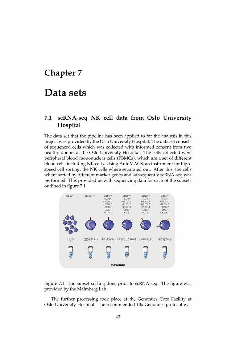
Eventually we end up with a feature-barcode matrix with UMI countsas the data in the matrix. Each gene is a feature and each cell has a barcodeso that we know which cell’s feature we have measured. For generatingthe sequencing libraries there exist a number of different protocols. In thisproject we used the recommended 10x Genomics protocol. The specifics ofour data sets are described in section 7.1.
2.4.2 Challenges working with scRNA-seq data
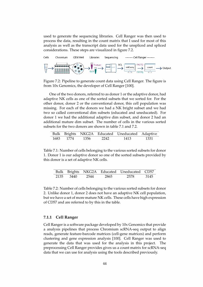
The high precision and resolution that the single cell approach providesus with, comes with a cost: single-cell data is much noisier than bulksequencing data. Two effects that are especially important are so calleddropouts and batch effects. The problem of dropout does not exist for bulk-RNA-seq data, because this data is generated by an average over a set ofcells. Batch effects exist also for bulk data, but the correction for this effectis different for scRNA-seq data. Here follows a description of these twoeffects.
11
Dropouts
Only 10-40% of the transcripts in a given cell are captured in currentscRNA-seq methods [34]. This means that all genes in all cells areundercounted. Genes which have very low levels of expression might bemeasured to be 0, even if these genes are actually expressed in the givencell.
Dropout is the phenomenon of having measured a 0, when the gene isactually expressed. This is therefore known as a technical 0, as opposedto a biological 0, where a gene is actually not expressed. However, asmentioned, this undercounting is present for all cells and all genes, notjust those that are lowly expressed and therefore risk resulting in a 0 value.
This means that scRNA-seq works as a kind of sampling method, anddropout is essentially undersampling of RNA molecules. This undercount-ing obscures many biological signals, such as gene-gene relationships [35],which makes working with raw scRNA-seq data very challenging.
Batch effects
If we perform scRNA-seq on one batch of cells, the gene expressionmight differ systematically from the gene expression in a different batch.This is known as batch effects and occurs because scRNA-seq data setsare generated in different laboratories at different times with potentiallydifferent techniques [36]. Since this is also a problem when studying bulkRNA-seq data, methods exist in well established bioinformatics packagessuch as limma [37] to tackle this. However, the problem of batch effects inscRNA-seq data is different than for bulk data. The main assumption in thebulk RNA-seq data approaches is that differences in mean gene expressionbetween batches is due to the batch effect and therefore should be removed.For scRNA-seq data this assumption is false and new, single cell specificmethods for dealing with batch effects have been developed [36] [38].
2.4.3 The need for bioinformatics
Despite the challenges described above, there have been a lot of interestingdiscoveries using scRNA-seq data [29]. The technology is constantlyevolving and new bioinformatics tools are being developed. To tackle theinherent challenges with the scRNA-seq data as described above, specifictools for analyzing this data have been developed.
scRNA-seq data is a transcriptional snapshot of a single cell. We needto use this data to infer other information, such as the differentiationtrajectories or imputed data matrices to tackle droput. Different statisticalmodels and bioinformatics tools have been developed for these purposes.A lot of the tools that previously were developed for use in bulk RNA-seq analysis can also be applied in the context of scRNA-seq data. But, asdiscussed, there are some characteristics which are specific to the single cellapproach and inherent to the data we are provided with by this sequencingmethod.
12
The data that we get from performing scRNA-seq is of a very highdimension: we have thousands of cells with expression levels acrossthousands of genes. It’s the high dimensional nature of the data thathas opened up the possibility to study cell states as a continuous geneexpression space, as opposed to consider it as a set of discrete states [11].However, the high dimensionality also poses some problems in terms ofinterpretation, visualization and computational complexity, in addition tothe problem of noisy data. Dimensionality reduction methods are thereforecentral to the analysis of scRNA-seq data sets. These and other methodswill be discussed in the next chapter, chapter 3. Following this, in chapter4, I will describe more specific bioinformatics tools for performing analysisof scRNA-seq data.
13
14
Chapter 3
Data processing and statisticalmethods
In this chapter I present some general data processing and statisticalmethods that have been used as part of tools and pipelines for analyzingscRNA-seq data that have been used in previously published research.These tools provide us with standalone analysis as well as the mathematicaland statistical models that underpin the scRNA-seq tools discussed inchapter 4.
3.1 Manifold model
The complexity of the scRNA-seq data, caused both by biological factorssuch as gene regulation and cellular behavior, as well as technical ones suchas those described in the previous chapter (see section 2.4.2), has called forsome simplifying assumptions. One such assumption that has proved towork well for scRNA-seq data is the so called manifold assumption [39][35]. The assumption is that the data actually comes from a relatively lowdimensional manifold. Under this assumption noise is treated as a high-dimensional phenomenon that can be alleviated by projecting the data ontothe lower dimensional manifold.
The justification for this assumption comes from known biology: thecell state space consists of smooth transitions and genes are regulated in acoordinated way. Transcription factors are proteins that control the rateof transcription for specific genes. From biology we know that sets oftranscription factors regulate modules of genes together. This means thatthe underlying structure of the cells, the gene expression vector space,can be embedded in a lower dimensional space without loosing too muchinformation. To put this in statistical terms we can say that the features (i.e.the genes) are not truly independent. This assumption is central to a set ofscRNA-seq tools, some of which will be described in more detail in chapter4.
15
3.2 Dimensionality reduction
As previously discussed, the data we get from performing scRNA-seq isof very high dimension (see section 2.4.3). For every cell we get a countof every gene. Combined with the single cell phenomenon of dropout thatcalls for some noise reduction efforts, this makes it necessary to performdimensionality reduction.
3.2.1 PCA
Principal component analysis (PCA) is a linear dimensionality reductionmethod that identifies a sequence of projections of the data that aremutually uncorrelated and ordered by variance [40]. These projectionsare known as the principal components, and the first principal componenthas the largest possible variance. By considering only the top principalcomponents, we project the data into a lower dimensional space and westill preserve a lot of the variance in the data. This helps to reduce thedimension of our high dimensional data and at the same time it removessome of the noise.
3.2.2 Diffusion maps
Diffusion maps (DM) is a nonlinear dimensionality reduction method[41] that has been used in multiple papers as a method when analyzingscRNA-seq data, both for dealing with the problem of dropout [35] andfor studying differentiation and trajectory inference [42]. Both these usecases are dependent on a metric for the distance between cells whichoriginally are placed in a high dimensional space. Diffusion maps embedsthe cells into a lower dimensional space, while still preserving somekey characteristics of the data it operates on. Cellular differentiation isconsidered a non-linear continuous process [43] and linear dimensionalityreduction methods usually will not be able to preserve the continuoustrajectories in the data [42]. Diffusion maps can be used to discover theunderlying structure of the data by providing us with an estimate of thelow dimensional phenotypic manifold of the data (see section 3.1).
3.2.3 t-SNE
t-distributed Stochastic Neighbor Embedding (t-SNE) is a dimensionalityreduction method introduced in 2008 [44]. It provides us with a twoor three dimensional embedding of the data and is frequently used forvisualization purposes. As the name implies, there is a stochastic elementto this method. The algorithm constructs a probability distribution withthe objective of preserving local relationships (the neighborhood). Sincethe embedding that results from running the method is based on thisprobability distribution, we will be provided with different results if werun the algorithm on the same data set multiple times. These differencesare often small and insignificant [45]. Over the last few years t-SNE has
16
become a well-established tool for use in biological papers for visualizationof genomics and transcriptional data [46] [47] and is currently one of themost commonly used technique in scRNA-seq data analysis [48].
3.2.4 UMAP
More recently, the dimensionality reduction method Uniform ManifoldApproximation and Projection (UMAP) has been proposed as an altern-ative to t-SNE for visualization of high dimensional scRNA-seq data [48].This method is based on manifold theory and topological data analysis [49][50] and has been tested on a variety of data sets in bioinformatics and otherfields [50]. In a 2019 comparison [48] between t-SNE and UMAP on theirability to produce meaningful representations, UMAP was found to pro-duce equally good representations of the cellular space, especially when itcame to separating out cell populations with very subtle differences defin-ing them. UMAP was also found to preserve more of the global structurethen t-SNE, and to preserve the continuity of cell subsets better. UMAPalso had shorter run time than t-SNE in general. How much faster UMAPwas, depended on the specific t-SNE implementation they compared it toas there exist numerous implementations of t-SNE. Consequently UMAPhas grown in popularity and has since been implemented in establishedscRNA-seq frameworks [8].
3.3 Artificial neural networks
Artificial neural networks (ANNs) are the main deep learning models anda major part of the field of machine learning [51]. The influence of ANNshas grown rapidly in recent years as they have proved to outperform anumber of models in a variety of areas. A standard so called feed forwardnetwork aims to approximate a function by learning the parameters ofthe model by updating the parameters based on the data we feed themodel. In this supervised case we need input-output pairs and we wantthe model to approximate a function that maps a given input to thecorresponding output. These models are called networks because theytypically compose together many different functions, which are modeledas a directed acyclic graph that describe how these are composed together.These chain structures are the most commonly used structures of neuralnetworks, and we aim to learn the value of the parameters in this modelto minimize the difference between the proposed output by the modeland the ground truth output. The “deep” part comes from the use ofmultiple layers of functions being connected. The layers in the middle ofthe models, which typically don’t have any obvious interpretations, arecalled hidden layers. Feed forward ANNs have not really been applied inany significant way in the field of scRNA-seq, however they provide thebasis for another type of ANN that recently has been applied, namely theso called autoencoders. These are described next.
17
3.3.1 Autoencoders
A more recent development in the field of neural networks are the so calledautoencoders [51]. These models are not dependent on us providing input-output pairs, but work in an unsupervised way. The goal of these modelsare not to approximate some mapping function, but rather to learn theunderlying structure of a data set. This is done by constructing both anencoder (that learns the representation) and a decoder (that uncompressesthe data again). By putting these two parts together, the autoencoderoutputs a reconstruction of the input. The learning process updatesthe parameters of the model to minimize the error (often squared error)between the original input and the reconstructed one. After training sucha network we can use the decoder part of the autoencoder to performdimensionality reduction. The decoder has then effectively learnt, in anunsupervised way, a way to represent the data in a lower dimensionalspace and consequently ignore the signal noise. Autoencoders have beenapplied for dimensionality reduction, data imputation and clustering inthe field of scRNA-seq [52] [53]. The application of deep learning modelsfor analysis of scRNA-seq is a field of growing interest [54]. Futureapplications of ANNs and the potential use of ANN models other thanautoencoders for analyzing scRNA-seq data will be discussed in moredetail in section 14.9.
3.4 Clustering
3.4.1 Louvain modularity
In many complex networks, such as the transcriptional representation ofthe cells that we get from performing scRNA-seq data, the data pointscluster and form relatively dense groups. We often refer to these groupsas communities and if we can compute these communities, we can usethis to find clusters of the scRNA-seq data. In 2008 Blondel et al.proposed a community detection method known as the Louvain methodfor community detection [55]. The method was first applied to a data setfrom the Belgian mobile phone network to identify language communities.It seeks to optimize the network modularity, which is a measure of thestrength of division, in a graph. Since going through all possible iterationsof nodes is computationally too expensive, the Louvain method is aheuristic method that first optimizes modularity locally and then iteratesto optimize the global community detection. The Louvian algorithm hasbecome one of the most popular and most cited algorithms for communitydetection [56] and is a central component in clustering tools that are oftenapplied in the field of scRNA-seq [57]. Phenograph is the most prominentexample of a clustering method based on Louvain modularity as describedin section 4.5.1.
18
3.4.2 Leiden
More recently the Leiden algorithm for community detection has beendeveloped as an alternative to the Louvain algorithm [56]. Just likeLouvain, the Leiden method can also be applied to optimize modularity.In the paper that introduced the Leiden algorithm, the authors identifiedsome problems with the Louvain approach. The main problem is thatit under certain circumstances can result in arbitrarily badly connectedcommunities. They therefore proposed their own method that guaranteeswell-connected communities based on some previous work [58] [59] [60]to improve the Louvain algorithm. The resulting method that they call theLeiden algorithm has gained some popularity and has also been applied inthe field of scRNA-seq data analysis [8].
3.4.3 K-means
K-means is a clustering method that has been around for a long time [61].The algorithm aims to partition the data points into k clusters. Each datapoint should belong to the cluster whose mean, known as the centroid,is closest to that given data point. This results in a partitioning of thedata space into regions based on distance to points in a specific subsetof the plane. The algorithm starts by choosing k random centroids, or itchooses these based on some heuristic or another domain specific process.It then assigns the cells to a cluster defined by the closest centroid. It thenrecalculates the centroids based on the actual data points in all the clusters.Then it reassigns the cells to clusters based on these new centroids. Thisprocess is iterated until it converges. This is a very simple and efficientclustering method, but it comes with some major drawbacks. One of thesedrawback is that k-means tends to produce equally sized clusters. Theseare spherically shaped due to the distance metric that is used to assign datapoints to clusters. The fact that we have to specify the k number of clustersin advance is also a drawback of this method. Despite this, k-means is awidely used method, often in conjunction with other more sophisticatedclustering methods.
3.5 Generalized additive models
Generalized additive models (GAMs) [62] are statistical regression modelswhere we have predictors and a dependent variable. The relationshipsbetween these follow smooth patterns that can either be linear or nonlineardepending on the data that the models are fitted on. GAMs strike a balancebetween the very complex and flexible black box learning algorithms (suchas ANNs) and the linear, biased and rigid linear models for regression [40].In the field of scRNA-seq, GAMs have been applied to the calculation ofgene trends [63], which are trends showing how the gene expression levelsdevelops as the cellular development proceeds. GAMs are used for thisbecause they are useful in deriving robust estimates of non-linear trends.
19
How GAMs can be applied to calculate gene trends discussed in moredetail in section 6.5.
20
Chapter 4
scRNA-seq bioinformaticstools
In this chapter I present some of the main bioinformatics tools that alreadyexist for conducting analysis of scRNA-seq data.
4.1 Data imputation
As discussed in section 2.4.2, one of the problems with single cell genomicsis that the measured counts only capture a small random sample of thetranscripts that are actually present in a given cell. Imputation is anapproach for dealing with sparse genomics data that is common in a varietyof fields in bioinformatics [64]. Imputation methods essentially replacesmissing values with substituted values that can come from varying sourcesand models depending on the specific method that is applied [39] [64]. Thesparseness of the scRNA-seq data comes in part from the undersamplingand dropout phenomenon that is inherent to scRNA-seq data. Howevernot all zeroes in the data matrix are equal. Some zeroes come from the factthat the given gene is actually not expressed in the given cell. This makessome traditional imputation methods, methods that have been applied instatistics generally and in other bioinformatics fields, unsuitable in this caseas a lot of these methods assume that all zeroes should be imputed and/orthat the non-zero values should not be changed.
A number of approaches for dealing with dropout and undersamplingin scRNA-seq data have been proposed based on a number of mathematicaland statistical models [35] [65] [52]. Broadly speaking they fall into twocategories: either they apply a model of the expected gene expressiondistribution to distinguish true zeros from dropouts in the data matrix, orthey apply a data smoothing method [64]. The most recently developedmethod discussed here, DCA, uses a deep learning autoencoder (seesection 3.3) and is a combination of these two categories.
21
4.1.1 MAGIC
Even if we only observe a small sample of the mRNA in a cell, we canstill make useful changes to the data matrix if we incorporate some basicbiological insights and some statistical and mathematical methods in ourapproach. Many of the genes we measure are redundant from a biologicalperspective because they are regulated together in a coordinated way. Thisis the realization that is central to the use of the manifold assumption asdescribed in section 3.1. This assumption was central to the developmentof the Markov affinity-based graph imputation of cells (MAGIC) methodthat was published in 2018 [35]. It exploits this underlying structure, themanifold, of the transcriptional data to impute missing and undercountedvalues. The main idea behind MAGIC is to learn the manifold of thescRNA-seq data and use it to recover the gene expression values. MAGICperforms data smoothing for scRNA-seq data based on each cell’s k nearestneighbors and thereby falls into the first of the two categories describedabove.
MAGIC is based on the use of diffusion maps to estimate the lowdimensional phenotypic manifold and looks at the neighborhoods in thisspace. Euclidean distance gives the incorrect neighbors because celldevelopment in the space twists and turns, as marker genes rise and fallin expression. Therefore cells are embedded into a graph structure andthe neighbors are considered based on how many steps away a cell is andweighted accordingly.
Imputing and denoising of the gene counts are done by filtering them assignals on this manifold. MAGIC denoises the data by sharing informationacross similar cells, and consequently it will also impute missing values(dropout), but it is not restricted to imputing only these values. MAGICessentially imputes values for each cell based on cells that are most similarto it by using the covariate relationships between genes as justified by themanifold assumption. This incorporates the biological insight discussedabove, that the gene set is not independent. This results in an imputed datamatrix with modified expression levels for the genes in the data matrix andcan be used for down stream analysis.
Validation
In the paper that describes MAGIC [35], the authors showed that theimputed data matrices outputted by MAGIC gave meaningful results fora lot of different applications. One of the main focuses in the paper wasthe method’s ability to recover gene-gene relations. Because of the highdegree of dropout, it is very unlikely to measure two individual genes inthe same cell. Gene-gene relations that are already known are thereforeoften impossible to see in the scRNA-seq data. By applying MAGIC todifferent data sets, these relations were restored.
22
4.1.2 SAVER
More recently SAVER was developed as an alternative imputation methodto MAGIC [65]. It’s development partly came from the observation thatMAGIC’s approach to imputation can lead to oversmoothing and removesome natural cell-to-cell stochasticity in the gene expression that actuallycaptures some meaningful biological signals. SAVER belongs to the firstcategory of imputation methods outlined above, and hence it applies amodel of the expected gene expression distribution. SAVER assumes thatthe count of each gene in each cell follows a negative binomial model andtakes a UMI count matrix as input. It then estimates the prior parametersand outputs an estimation uncertainty (unlike MAGIC) and a matrix ofimputed gene expression values. SAVER was tested on a number of datasets and performed well in recovering gene expression values and showedimprovements also compared to MAGIC on downstream analysis.
4.1.3 DCA
Deep count autoencoder network (DCA) was proposed in a 2019 paper[52] as a new method for denoising of scRNA-seq data. The maincomponent of this method is a deep learning autoencoder (see section3.3.1)that compresses the scRNA-seq data using specialized loss functionstargeted towards scRNA-seq data. Since the compression forces theautoencoder to learn only the essential latent features, the reconstructionignores non-essential sources of variation such as random noise. Theneural network model underpinning DCA is built so that it learns the gene-specific distribution parameters by minimizing the error. The compressionof the representation performed by the decoder causes it to learn gene-gene dependencies because some genes can be considered as dependentfeatures. By default DCA uses three hidden layers which allows for non-linear mappings.
One major advantage of DCA is that it allows the user to decidethe noise model. As the field of scRNA-seq analysis keeps developingthe underlying statistical assumptions researchers build there analysison are under constant discussion and it has been suggested that theapparent zero-inflation in scRNA-seq data, that a lot of methods assume,is not present when using UMI counts and that it also depends on thenormalization method used[2] [66]. It would therefore be useful to letthe users themselves decide on a noise model based on the assumptionsthey make. This also helps keep the method relevant if new insights areencountered as these easily can be incorporated into DCA. These aspectswill be discussed in more detail in section 13.1 and section 14.9. DCAis based on the state-of-the-art deep learning Python library TensorFlowand its higher level API Keras [67] which provides it with very goodperformance.
23
4.2 Trajectory inference
Trajectory inference, also known as pseudotemporal ordering, is techniqueused to determine the fate and the dynamics of cellular differentiation.One important concept in this field is pseudotime. The concept ofpseudotime was introduced in one of the early trajectory inferencealgorithms, Monocle, which since then has developed into Monocle 2 [68].Pseudotime measures a cell’s biological progression: later in pseudotimemeans that the cell is considered more mature and later in developmenttowards its terminal state. This same concept has since been usedin a number of newly developed tools for analyzing trajectories anddifferentiation by studying scRNA-seq data [1] [63]. Trajectories inferredfrom scRNA-seq data can unveil how gene regulation governs cell fatedecisions and a number of methods have been developed to this end.
According to a 2019 comparison of trajectory inference methods [69],50 different methods have been developed since 2014. In this paper theycompared the methods both by using a synthetic dataset, which providesthe most exact measure for comparing to a reference result, and by usingreal datasets, which tells us about the biological relevance of the analysis.This comparison concluded that a method called Slingshot predicted themost accurate trajectories. PAGA was another method that seemed toperform well in this comparison. Generally, it found that Slingshot workedbest for inferring simpler trajectory structures, while PAGA tended to dobetter if the underlying trajectory was more complex. The analysis in thepaper indicates that some of the methods are complementary and that onepreferably should choose a method based on the underlying data if one hasadditional insight into its structure.
The trajectory inference methods considered in this comparison tendto model differentiation as a series of discrete states and deterministicbifurcations [63]. As discussed in section 2.1, this view of differentiationdoes not fit with more recent developments in biology and conveysa limiting view of how differentiation progresses. The most recenttrend in trajectory inference methods is to model the distribution of acell population across a continuous cell state coordinate [12]. PAGAincorporate some of these aspects by generating a graph-like map of cellsthat preserve continuous structures in the data. Methods, which are notincluded in the comparison mentioned above, have been developed sincethen to incorporate this biological insight more explicitly. Palantir [63] isone of these methods.
4.2.1 Wanderlust
Wanderlust [43] was introduced in 2014 as one of the earlier developmentsof trajectory inference methods in the field of scRNA-seq. It is a linearmethod and only provides a trajectory inference if all the cells can beconsidered part of the same branch, i. e. it only provides us with anordering of the cells along a fixed topology that is predefined. This istypical of the early methods that were developed. Other early methods
24
suffered from the requirement of the user to specify the number of branchesand cell fates as a parameter. Since 2014, a number of new methods havebeen develop that have proven better at identifying known trajectories inwell-studied systems and at identifying trajectories in synthetic data sets[69].
4.2.2 Monocle 2
Monocle 2 [70] [68] [71] first learns the overall trajectory topology through amachine learning based dimensionality reduction method called reversedgraph embedding (RGE) [72]. The RGE method learns a function that mapsdata points in a high-dimensional space to points in a lower dimensionalspace. Monocle uses this to construct the graph that constitutes thetrajectory topology, and it then places each of the cells in the data setat its proper place in the trajectory. This results in an ordering of thecells and a basis for calculating pseudotime along the different trajectories.Monocle 2 requires explicit specification of the terminal states, which limitsits applications if this information is unknown or if this is the exact thingthat we want to calculate. In another comparison where known trajectoriesand gene expression trends in human hematopoisis was studied, Monocle 2was also shown to perform worse in recovering the differentiation lineagescompared to Slingshot, PAGA and Palantir [63]. Monocle 2 was also foundto have worse performance on data sets as the number of cells increased.This indicates some fundamental limitations in its application especiallyas the field moves toward methods that are able to take advantage of therapidly increasing amount of scRNA-seq data that is available. This is theopposite of most other methods [73], which tend to perform better givenmore data.
4.2.3 Slingshot
Slingshot [73] is a more recent method for inferring cell developmentaltrajectories in scRNA-seq data. It overcomes some of the limitations ofboth Wanderlust and Monocle 2. Among other things it does not requireexplicit specification of the terminal states. Slingshot first constructs aminimum spanning tree (MST) on cell clusters to identify the topology ofthe trajectory structure, i. e. to identify the lineages. It then calculates thepeudotime of each cell.
4.2.4 PAGA
Partition-based graph abstraction (PAGA) [74] is one of the more recentlydeveloped methods for trajectory inference. As mentioned above it hasbeen shown to give good results on a variety of data sets. PAGAprovides an interpretable graph-like map of the data manifold. Thisgraph is based on the connectivity in this partition. While Palantir andSlingshot automatically can determine the terminal states, PAGA requiresspecification of the PAGA clusters that belong to a particular lineage.
25
4.2.5 Palantir
Palantir is one of the most recent developments when it comes to trajectoryinference method [63]. It was developed by the same lab as MAGIC(see section 4.1.1) and in some ways it is based on the same underlyingassumptions of the existence of a lower dimensional phenotypic manifold.Similar to MAGIC, Palantir uses diffusion maps to estimate this manifold.Palantir was designed to investigate cell plasticity and fate decisions,based upon a continuous, probabilistic model for a cell’s potential to reachdifferent cell fates. Palantir treats cell-fate as a probabilistic process. A cellis not assumed to commit to a given path in a bifurcation of trajectories,but each cell is assigned a probability of ending up in each of the terminalstates that the algorithm identifies. These probabilites are known as branchprobabilities.
The aim of the model is to build in the assumption of the continuousnature of cell fate and differentiation as discussed above. The actualdifferentiation process is modeled as a Markov chain, which is turnedinto an absorbing Markov chain where the terminally differentiated cellsare the absorbing states. Based on the graph structure and the Markovchain the cells are ordered and the pseudotime of each cell is calculated.Pseudotime is a measure of the distance between the starting cell and anygiven cell. Based on the branch probabilities, Palantir calculates the entropy(the negative log of the probability mass function). Higher entropy meansthat the given cell has a higher potential to reach different terminal states.The entropy is therefore a measure of differentiation potential (DP).
DP captures an aspect of the continuity in cell fate determination. Thisprovides us with a better view of differentiation processes compared towell-defined bifurcations. Cell fate is modeled as a stochastic process andPalantir requires the least amount of a priori biological information amongthe methods discussed here. We only need to provide the starting cell aswell as the data matrix as input and we are provided with pseudotime,branching probabilities and differentiation potential as output.
In the paper where Palantir was presented [63], the authors comparedit to the most commonly used competing methods, such as Slingshot andPAGA, and found it to provide better results when inferring trajectoriesin human hematopoiesis, which is a very well-studied system where theinferred trajectories easily can be tested against known biology.
4.3 RNA velocity
So far we have looked at methods based on studying the RNA abundanceof the cells. All of these methods analyze a data matrix where we have thegenes and we have a count for each of these genes for each of the cells inthe sample. As discussed above (see section 2.4.3), this is just a snapshot ofthat cell and it does not in itself tell us anything about the dynamics of thecell in terms of differentiation. The trajectory inference methods infer thisinformation from looking at the landscape of cells that all the cells make up.
26
A different approach for studying the dynamics of cellular development,called RNA velocity, was proposed in 2018 [15].
As alluded to in the background chapter about RNA splicing, thedifference between unspliced and spliced mRNAs in a given cell can beused to predict the cell’s cellular state progression. This adds a new layerof information to the analysis. The RNA velocity calculation is based onlooking at not only the gene-cell matrix, but by looking at the transcriptlevel counts. It looks at both unspliced and spliced RNA and calculatesthe first time derivative of the difference in abundance between these aswell as at the degradation of mRNA. The resulting metric is called RNAvelocity. This can then be used to identify the dynamics and direction ofdifferentiation. More details on how to combine this velocity vector withother analysis tools and how to visualize the results will be discussed insection 6.11.
4.4 Factor analysis
Because of the very high dimensional nature of the scRNA-seq data itwould be useful to be able to get a metric for the expression values of aset of genes instead of only considering individual genes. To capture thesetype of aggregated values, known as factors or metagenes, we can use socalled factor analysis.
Factor analysis is a statistical analysis that aims to describe thevariability among many observed factors in terms of a preferably lowernumber of unobserved variables. In our case of scRNA-seq data the manyobserved factors are the gene expression levels that we have measured,and the lower number of unobserved factors can be a functional factor thatconsists of a list of genes which together represent a given functional role.The factor is then essentially a weighted list of the genes that go into thatgene list. The unobserved factors are metagenes that vary smoothly andare less skewed compared to the expression of single genes. They shouldbe able to identify some broader trends and are not that dependent on thevalue of one single measurement.
The problem of factor analysis is essentially a factorization problem.We want to factorize our scRNA-seq data matrix to enable this analysis[75]. A lot of different methods have been proposed for achieving thisfactorization. Typically these are based on singular-value decomposition(SVD), regression or principal component analysis (PCA)[76]. Howeverthese methods do not model error in the way the gene sets that weuse as factor are defined and they do not take into account unannotatedfactors. f-scLVM is perhaps the most prominent factor analysis methoddeveloped for scRNA-seq and its development was in part motivated bythese limitations of the already existing methods [76].
27
4.4.1 f-scLVM
Factorial single-cell latent variable model (f-scLVM) is a factor analysismethod that not only computes estimates of the relevance of the factorsit infers, but it also lets us predefine gene set annotations which resultsin refined factors. We can provide a set of gene lists (these can comefrom various databases, see section 4.7) which constitute the annotatedfactors and f-scLVM infers additional unannounced factors based on thevariability in the data.
In the paper where it was presented [76], f-scLVM was shown to suc-cessfully decomposes scRNA-seq datasets into interpretable components.Since the method provide us with a metric for different factors and theircontribution to the variance in the expression levels, it can also be used toregress out the effect of given factors. One example of this is the use off-scLVM to correct the expression matrix for the effect of the cell cycle asdone in various published papers [13].
4.5 Clustering
4.5.1 Phenograph
Phenograph is a clustering method that algorithmically defines phenotypesin the high-dimensional scRNA-seq data [57]. It infers transcriptionallydefined clusters in an unbiased way. Phenograph is based on the Louvainmodularity (see section 3.4.1). After creating a weighted graph where theweight is dependent on the neighborhood of the two connected nodes (a setof cells), the Phenograph algorithm uses this community detection methodto divide the graph into parts which then constitutes the final clusters.Phenograph is currently one of the most established methods for scRNA-seq cluster analysis and is implemented in the most established toolkits [8][77] and have successfully been applied in a number of scRNA-seq dataanalysis papers [63] [48].
4.5.2 AP Clustering
Affinity propagation (AP) was introduced as a clustering method in 2007[78]. It is based on the idea of passing messages between data points. Thesemessages are real-valued and are exchanged until a set of exemplars andtheir clusters emerges. AP clustering has showed useful for clustering insome fields of computational biology. In the paper where AP clusteringwas introduced, they applied it to identify genes in expression data oftranscripts of possible exons, and to identify regulated transcripts. APclustering was first implemented in R [79] for use in bioinformatics.
4.6 Differentially expressed genes
Differentially expressed genes (DEG) are genes which are significantlyhigher or lower expressed in one sample compared to another sample.
28
This can for example be used to compare the gene expression of twophenotypic clusters or arbitrarily defined sets of cells. The need to calculatedifferentially expressed genes is also present in the context of bullk RNA-seq, and there are many well-established methods for performing this typeof analysis. However, it is unclear whether the methods developed for bulkRNA-seq can be applied reliably to scRNA-seq data [80]. Therefore therehas been recent developments to build single cell specific DEG analysis,such as SCDE [81] and MAST [82]. Both these methods were developedwith the objective of dealing with the single cell specific challenge ofdropout.
4.6.1 SCDE
Single-cell differential expression (SCDE) [83] is a single cell specific Rpackage developed by Kharchenko et al. for performing analysis ofdifferentially expressed genes (DEG). The Bayesian approach to single cellDEG analysis that this packages implements was described in a 2014 paper[81] and have proved useful for this purpose [80].
4.6.2 Bulk RNA-seq DEG methods
Multiple bulk RNA-seq DEG methods have previously been developed.The most prominent of these have also been implemented for scRNA-seqdata through toolkits such as Seurat (see section 4.12) and Scanpy (seesection 4.11).
4.7 Databases
4.7.1 Gene Ontolgy
Gene Ontology (GO) is a resource of annotated genes and gene productsthat provides us with a unified definition of terms that represent geneproduct properties [84]. Traditionally, different areas of biology, such asgenetics and biochemistry, used different terminology even if they agreedon the underlying concepts. GO was developed to deal with this and theconsequential lack of interoperability of different genomic databases. Thereare three domains that the GO terms in the ontology can belong to: cellularcomponent, molecular function and biological process. 85 % of humanprotein-coding genes have GO annotations.
4.7.2 Kyoto Encyclopedia of Genes and Genomes
Like GO, Kyoto Encyclopedia of Genes and Genomes (KEGG) is a database which contains information about gene functions in the context ofmolecular pathways in the cell [85].
29
4.8 Gene set enrichment analysis
If we have a gene list and want to understand which functions or propertiesthis gene lists encompasses, we can use gene set enrichment analysis(GSEA). This is a method where we perform a statistical test to see howsimilar the input gene list is to a predefined database of gene lists. If alist in the predefined database is statistically significantly over-representedin the input gene list, we say that this list is enriched for that input [86].The predefined set of gene lists can come from any source, but typicallywe use GO, KEGG or another established functional database. The inputgene list is typically constructed based on some shared property amongthe given genes in an experiment, for example genes that show the sameexpression pattern or genes which are differentially expressed between twosets of cells.
4.8.1 GO enrichment analysis
Gene ontology enrichment analysis (GOEA) is when we perform enrich-ment using the GO data sets. There exists a number of tools for performingthis type of analysis. GOATOOLS [87] was developed in 2018 and is a Py-thon library. There also exists R packages to perform this analysis such asclusterProfiler [88].
4.8.2 KEGG enrichment
KEGG enrichment analysis is used to extract relevant functional featuresof gene lists using the KEGG database. There exist a number of packages,mostly in R, to perform this type of analysis. clusterProfiler [88] is one ofsuch package.
4.9 Correcting for batch effects
Batch effects are a problem when studying scRNA-seq data sets thathave been produced in different laboratories and at different times. Asmentioned in section 2.4.2 the methods developed previously to thedevelopment of single cell specific solutions to this effect, was mostly basedon assuming that the cell populations were similar across batches so thatthe mean expression values could be used to remove the batch effects.This assumption does not hold true and a single cell specific method basedon the detection of mutual nearest neighbors (MNNs) has been proposed[36]. These mutual nearest neighbors are cells that have similar expressionprofiles across different batches. We can then use the matching of mutualneighbors to correct for the batch effects. This approach was originallyimplemented in R as mnnCorrect in the scran package [89] [36], but hassince then also been implemented in Python [38].
30
4.10 Deconvolution
Despite the rapid advancement in scRNA-seq technology, performingscRNA-seq heterogeneous tissues still requires labor-intensive protocols.This has hindered their establishment in a clinical setting. Computationalapproaches have therefore been developed to infer the abundance ofdifferent cell types in samples on which bulk sequencing has beenperformed. In addition to making the analysis of tissue samples fasterand cheaper, the computational deconvolution approaches also lets us gaininsight into the composition of pre-existing data sets.
Deconvolution of the cell composition of a sample can be consideredas a factorization problem [90]. Some of the most recently developeddeconvolution tools [91] [92] rely on a signature matrix that capturesthe gene signatures of the different cells whose abundance we want tocompute. CIBERSORT is perhaps the most well established deconvolutiontool and has among other things been used to deconvolute the immune cellcontent in various cancer types [91] [93].
In addition to deciding on the actual factorization method, the mainproblem in the field of deconvolution is to create an accurate signature mat-rix and the construction of this has been one of the main challenges. Signa-ture matrices have previously mostly been constructed by considering ex-isting data bases of marker genes and sequenced cells [94]. More recentlyhowever, it has been proposed that we can use single cell data to create thismatrix [95]. This may allow us to combine the new insight provided byscRNA-seq data with the advantages of studying bulk sequencing samplesand analyzing them using computational deconvolution.
4.11 Scanpy
Scanpy is a toolkit for analyzing scRNA-seq data that was developedto integrate different scRNA-seq data tool [8]. The motivation was todevelop a scalable toolkit to deal with the increasingly large data setsthat are generated by the rapidly increasing use of scRNA-seq. Wheremost frameworks and toolkits previously had been developed in R, theresearchers behind Scanpy opted for a Python-based implementation.Scanpy continues to be developed and has gotten a lot of tools added toit since it was first published. Some of the bioinformatics methods thatI have discussed so far has been implemented as a part of Scanpy andsome methods that previously only was found as R packages has also beenimplemented in Python to make it compatible with Scanpy [96].
4.12 Seurat
Seurat [77] is an R toolkit developed to enable analysis of scRNA-seq data.It is in many ways the R equivalent of Scanpy and enables the integrationof various scRNA-seq tools. It was initially develop previous to Scanpy
31
and offers many of the same features in terms of preprocessing, clusteringand visualization.
32
Part II
Methods
33
Chapter 5
Technologies
5.1 Programming languages
For this project I have primarily used Python and R for development andfor incorporating existing tools into my own scripts. I used Conda as thepackage manager and took advantage of Conda’s feature of environments.Most of the packages and libraries I used are available through Condausing various repositories. Some of the most important Python librariesI have used include Pandas for data frames, Numpy for matrices andmatrix operations, and PyQt for the graphical user interface components ofSingleFlow. PyQt is the Python binding of the cross-platform GUI toolkitQt. R provided me with some of the statistical libraries and some of thebioinformatics methods discussed previously. In order to access packageswritten in R, I used rpy2 in Python, which is an interface to R from Python,or simply ran R scripts independently as separate Nextflow processes. Toperform the initial exploration of the data and to test out the different toolsthat I have used, I used Jupyter notebooks.
For the version control and to facilitate development, I used GitHub.The final version of the SingleFlow code is available at https://github.com/hernet/SingleFlow. For some of the more computationally intensivecalculations, I used the Abel server which the University of Oslo gaveme access to. Nextflow is the fundamental framework that SingleFlowwas built on, in order to build reproducible, automated and modularworkflows. This framework ties together the use of different tools andprogramming languages. Nextflow is described in more detail in section5.2.
5.1.1 Dependencies
SingleFlow has a set of software dependencies. Fundamentally it requiresthe Java Virtual Machine (JVM) and Java 8 or later to run Nextflow. It alsorequires the installation of the workflow manager Nextflow. The requiredPython and R packages, and the specific versions that I have used, are listedon the GitHub page (https://github.com/hernet/SingleFlow).
A bioinformatics pipeline consists of a number of different tasks that canbe used in various sequences and combinations. The many permutations apipeline can follow leads to a certain complexity. There exist a number ofbioinformatics pipeline frameworks to deal with the problem of handlingthe execution of a large number of different software packages that mightnot be easily bundled together [97]. These frameworks generally work asworkflow management systems.
Nextflow is perphaps the most prominent example of such a frameworkin the bioinformatics discipline [98] [97] and is the one I decided to usefor this project. In the field of bioinformatics and biostatistics there exist anumber of specialized software packages in different languages to performspecific analyses. The methods that any given pipeline uses might bevery specialized and might be most easily implemented by accessinglibraries available in a specific scripting language. Tools have thereforebeen developed in specific languages to easily incorporate already existingpackages. One task might require the use of R, while others might requirethe use of Python, because of the libraries or APIs available in the respectivelanguages. Through Nextflow’s management system we can easily managethese different processes and integrate them. Nextflow also providesefficient parallel execution and traceability [98].
Nextflow implements the dataflow programming paradigm [99]. Thisparadigm models the data flow as a directed graph and ensures that tasksare automatically started once they receive data through the defined inputchannels. This allows for very effective parallel execution in a pipeline. Thecomputational dataflow is defined by implementing separate processes, asthey’re called in Nextflow, for a given module, and then define channelsand connections between these. One process can for example performdimensionality reduction and then output this to a channel that is thenused as input to a downstream process that requires a lower dimensionalrepresentation of the data set. The downstream process won’t start untilthe channel whose content it takes as input has received the data fromthe upstream process. If multiple processes both depend on receiving thisdata (but don’t depend on each other) they can be started simultaneouslyonce the dimensionality reduction is performed and their execution willbe parallelized. Nextflow also provides us with statistics and figuresdescribing the dataflow and the execution of the various processes. We canfor example have Nextflow generate a flowchart of the processes that goesinto the analysis or make it report run time, CPU usage and other metrics,if we provide the appropriate parameters when running the pipeline.
36
Chapter 6
Bioinformatics methods
To build the SingleFlow pipeline I worked closely with the MalmbergLab to determine what kind of analysis we would want to perform onthe scRNA-seq NK cell data set. The biological insight gained from thiscollaboration, formed the basis for deciding which tools I should includeand which biological questions we would try to answer using that analysis.
Data cleaning was implemented by allowing the user to decide theminimum number of molecules a cell must have in order to be consideredpart of the analysis and by deciding the minimum number of cells thatmust exhibit the gene for the gene to be one of the features that willbe considered. This type of filtering has been proposed in a number ofprevious studies [63] [35] [96]. It also provides the user with some flexibilityin choosing the parameters for the filtering.
As in other contexts where we are dealing with high dimensionaldata, feature selection is an important step in the analysis of scRNA-seq data. As mentioned above, the features in this context are thegenes. The gene expression vector of a cell puts the cell in a very highdimensional space. Some genes are filtered out during data cleaning, whichtherefore constitutes the initial feature selection. Other feature selectionmethods were also implemented based on looking at variable genes anddifferentially expressed genes. When performing the gene set enrichmentanalysis we did feature selection by only looking at those genes which hadlog2-fold change greater than a given number (we used 1 for the results inchapter 11) and that where significantly differentially expressed.
I also implemented normalization methods based on what can beconsidered the standard pipeline for scRNA-seq preprocessing [96] [2].I implemented the normalization methods that come with the Palantirlibrary, which performs normalization of the gene expression based onthe total expression of the gene in the sample. I also implemented logtransformation, which is widely used as a transformation step in scRNA-seq analysis. Since it recently has been suggested that this standard
37
pipeline of preprocessing might suffer from some flaws [2] [66], I alsoincluded the option to not normalize the data at all. Other future changesto this will be discussed in section 13.1.
6.2 Dimensionality reduction methods
I implemented a set of dimensionality reduction methods, both for visualiz-iation purposes and for preprocessing the data for further downstream ana-lysis. All the methods discussed in section 3.2 were implemented becausethey can serve different purposes and they can complement each other. Inthe suggested analysis in the MAGIC paper for example [35] they performboth PCA (linear dimensionality reduction) and DM (non-linear). The PCAwas used for initial noise reduction and the non-linear diffusion maps wasused to estimate a lower dimensional manifold that could then be used forfurther down stream tasks. This order of applying dimensionality reduc-tion method is also the default in SingleFlow. However SingleFlow’s flexib-ility allows for alternative execution paths and to integrate other methods,such as the recently proposed GLM-PCA [2]. This will be discussed in moredetail in section 14.6. t-SNE and UMAP are mostly used for visualizationpurposes and consequently fits together with the other tools by providingembeddings for us to incorporate other metrics into.
6.3 Gene expression imputation
As discussed in detail in section 4.1 the problems that the undercounteddata that scRNA-seq provides us with has shown to be alleviated byvarious imputation methods. As part of the development of SingleFlow,MAGIC was the primary imputation method that I implemented. The morerecent methods of SAVER and DCA were also implemented as alternativeimputation methods. The data outputted from any of these methods canbe used for computing downstream analysis. It has however recently beensuggested that imputation methods are prone to generate false positiveor irreproducible results when computing differentially expressed genesusing the imputed data [64]. The default workflow of SingleFlow thereforedoes not use the imputed data matrix for this computation. As with theother workflow specifics this is also something the user can change byusing the parameters when running SingleFlow.
6.4 Differentiation trajectories
In order to gain insights into NK cell differentiation SingleFlow neededto implement differentiation trajectory inference methods. As discussedin section 4.2 there exist a number of tools for this, all with their owndraw backs. Palantir is the primary method I used when developingSingleFlow. It is one of the most recently developed methods andincorporates important biological insights in its statistical models. It has
38
shown to work better at certain data sets than methods such as Slingshot[73] and PAGA [74] [63]. Palantir also provides us with a probability of eachcell to end up in each of the inferred terminal states, which gives us a usefulmetric for weighing the cell’s contribution when computing gene trendsas discussed in section 6.5. Another advantage of Palantir compared tosome of the other methods is that the only input that we need to give is thestarting cell, i.e. the cell that is assumed to be the least developed cell. Forthe specific NK cell user scenarios in this project we identified starting cellsby looking at the lowest expression of genes that we know from biologyto be associated with cellular development in NK cell biology. We usedthe imputed data matrix to identify the cell with the lowest (or highest,depending on the gene) expression of a given gene so that the specific cellwould not be some outlier in the middle of the manifold, but a cell thatresides in a region where the expression of the given gene is low.
Since SingleFlow is designed to be a modular pipeline, long-termwe can easily implement potentially all of the other trajectory inferencemethods discussed. We can also easily compare the results from these,both the actual resulting analysis and trajectories, and their performancein terms of running time and resources required. I have implemented theoption to run PAGA and Slingshot using SingleFlow to allow the user tocompare the results of the most prominent trajectory inference methods asdiscussed in section 4.2.
6.5 Gene trends
The computation of differentiation trajectories and the subsequent pseudo-time calculation provided by the previously described methods in section4.2 and section 6.4 provides us with an ordering of the cells. In order tostudy how gene expression levels develop as the cellular development pro-gresses, I combined this ordering with the gene expression levels of the cellsto produce gene trends. These trends showed us how the expression levelsof the different genes develop with pseudotime. These trends were calcu-lated by fitting a GAM, and weighing the contribution of the cells to theexpression at the given pseudotime based on their branch probabilities (ascalculated by Palantir) so that cells with a higher probability of committingto a given trajectory contributes more to the gene trend for that trajectory.SingleFlow lets us fit a GAM for each of the lineages identified by Palantirso that we end up with a trend for each gene for each of the lineages. GAMshave been found to produce robust trends [63].
Initially the gene trends were only computed with MAGIC imputeddata and the trajectory inference as calculated by Palantir as described inthe Palantir paper [63]. Imputed data is used here to avoid the effect ofdropout to interfere with the computation of the gene trends. SingleFlowallows however for the use of data that has been imputed using othermethods, or the use of data that has not been imputed at all. We can also useother pseudotime or trajectory inference methods, but to fit the GAM weneed a metric for weighing the cell’s contribution to the model fitting. With
39
it’s probability metric Palantir provides us with this. When referring to thecomputed gene trends we call the trends from pseudotime 0 to pseudotime1, i.e. the whole trend that we compute, the global gene trends. As I discussin more detail in section 9.2.3, I also implemented a method to zoom in ona specific range of pseudotime providing us with the local gene trends.
6.5.1 Clustering of gene trends
After computing the gene trends of potentially hundreds or even thou-sands of genes it will be interesting to see if there are certain genes whichinhibit a similar pattern with respect to their trends of expression level aspseudotime progresses. Based on known biology we expect sets of genesto be expressed in a similar pattern. We can identify the different waysin which genes and sets of genes can develop with cellular developmentby clustering the gene trends. I performed this clustering by using Pheno-graph (see section 4.5.1) as suggested in previous work [63]. After cluster-ing the gene trends SingleFlow performs normalization before it computesthe standard deviation and the mean of the gene trends in each cluster.Each of the clusters constitutes a list of genes that can be used for furtheranalysis, such as gene set enrichment analysis to identify which biologicalprograms these trends correspond to.
6.6 Single cell clusters
There exist a variety of methods for clustering. Phenograph is perhaps themost established one in scRNA-seq data analysis and the one I used as theprimary clustering method for this project. I also included other clusteringmethods, such as AP clustering and k-means clustering. For the NK cellbiology application we only used k-means in order to confirm the clustersidentified by Phenograph, by using the number of clusters Phenographidentified as the k input parameter to k-means.
6.7 Gene set enrichment analysis
The primary source of functional information in the gene set enrichmentanalysis SingleFlow provided in this particular study was from the GeneOntology (GO) database (see section 4.7.1). I implemented the Pythonlibrary GOATOOLS [87] to perform the enrichment analysis. I also addedKEGG enrichment (see section 4.7.2) as an alternative. In SingleFlow geneset enrichment can be performed down stream of primarily two processes:gene trend clustering and differential gene expression analysis. Havingidentified the clusters of gene trends SingleFlow allows for the enrichmentof the different clusters to identify the molecular programs that follow thetrend corresponding to that cluster. By performing gene set enrichment onthe differentially expressed genes between two clusters, we can get a higherlevel description of what separates the clusters.
40
6.8 Factor analysis
In order to get a metric for a set of genes I implemented a factor analysismethod (see section 4.4) as part of the pipeline. We can obtain gene listsfrom for example GO for specific biological functions that we are interestedin studying. I used the f-scLVM method implemented in the pythonpackages slalom for the factor analysis [76]. This package has been usedin a number of other papers, for example in the Palantir paper [13].
6.8.1 Cell cycle correction
One example of the use of factor analysis is its use in correcting the geneexpression matrix for the influence of cell cycle effects. The following GOannotations were used to quantify the cell cycle’s effect on gene expressionin the Palantir paper [13] and I used the same terms when implementinga cell cycle correction process in SingleFlow: M phase (GO:0000279), DNAreplication (GO:0006260), chromosome segregation (GO:0007059), M phaseof mitotic cell cycle (GO:0000087) and organelle fission (GO:0048285).
6.9 Differentially expressed genes
SCDE was used to compute differentially expressed genes as this is a singlecell specific method that has shown good performance as discussed insection 4.6. The results of the DEG computations were plotted on so calledvolcano plots. Volcano plots are used to identify changes in large data setsand has the fold change, which is a quantify of how much a measurementhas changed, of the expression of the given gene on the x-axis and thesignificance of the result on the y-axis. The fold change is shown as log2 ofthe fold change and the significance is -log10 of the computed p-value. Onthese plots SingleFlow highlights the genes that show a fold change largerthan a defined value as well as have a p-value lower than a given value.These cutoff values can be defined by the user or the default values of log2fold change greater than 1 and p-value lower than 0.05 can be used.
6.10 Deconvolution
I used the scRNA-seq data to construct the signature matrix that sub-sequently was used as input to CIBERSORT to perform the deconvolutionof inputted bulk RNA-seq samples. To create this signature matrix we needto identify the cell types that we want to deconvolute from the bulk RNA-seq sample. It is up to the user of SingleFlow to specify the cell identitiesthat need to be deconvoluted. It could be from performing one of the clus-tering methods and consider each of the clusters as its own cell type, forexample. Since we typically have multiple sorted subsets and their scRNA-seq data as input we could also consider these sorted subsets as the celltypes in the deconvolution analysis.
41
Following the identification of the cell types we have to identify themarker genes, i.e. the genes whose expression value to the largest degreeseparate these cell types. This was achieved by looking at the differentiallyexpressed genes between the different cell-type identities as well as thehighly expressed genes in the scRNA-seq data for these cells. Based onthis we then had expression values for a set of marker genes for cells ofdifferent types, this is then used to construct the final signature matrix thatconsists of values for each marker gene for each of the cell types to facilitatethe deconvolution of these cell types in the bulk sample.
As mentioned in section 4.10 CIBERSORT is one of the most commonlyused deconvolution methods and as suggested in [95] it can be combinedwith scRNA-seq data by constructing a signature matrix in a similar wayto the preceding description. CIBERSORT is therefore the method usedfor this project, but any other deconvolution method could potentially bepaired with the signature matrix we construct.
6.11 Velocyto
In order to calculate the RNA velocity (see section 4.3) of the cells in ourdata set, I used the command line tool velocyto [15]. Velocyto was randirectly on the output of Cell Ranger which is the software packaged thatwas used to generate the scRNA-seq data as discussed in 7.1.1. The outputof velocyto includes, in addition to the count matrix, all the informationabout which specific transcripts that was sequenced and therefore alsothe abundance of the spliced versus the unspliced version of the genetranscript. This was all outputted to a .loom file. I imported thisinto Python to analyze it further using the velocyto python library. Iimplemented a calculation of the velocity vectors and calculated locallyaveraged vector fields because our data sets typically (as in the NK celluser scenarios) consists of many thousands cells. These vectors werethe projected onto same t-SNE or UMAP embedding that is used forvisualizing other analysis as well. This allows us to visualize the RNAvelocity in the same tSNE plot that have visualized the cells in. All of thisis implemented as a process in SingleFlow and was applied in the NK celluser scenarios to determine future cell states.
6.11.1 Identify most important genes
To expand on the analysis provided by velocyto, I implemented a methodto identify the individual genes that contribute the most to the vectorswith the largest magnitude. Since the vectors we are projecting onto theembedding is based on the contribution from a neighborhood of cells, Ifirst identified the cells in the neighborhoods that gave rise to the highestmagnitude vectors. I then extracted the number-of-genes dimensionalvectors for each of these cells and identified the genes that contributedthe most to these vectors. The resulting genes were reported as the mostimportant genes.
42
Chapter 7
Data sets
7.1 scRNA-seq NK cell data from Oslo UniversityHospital
The data set that the pipeline has been applied to for the analysis in thisproject was provided by the Oslo University Hospital. The data set consistsof sequenced cells which was collected with informed consent from twohealthy donors at the Oslo University Hospital. The cells collected wereperipheral blood mononuclear cells (PBMCs), which are a set of differentblood cells including NK cells. Using AutoMACS, an instrument for high-speed cell sorting, the NK cells where separated out. After this, the cellswhere sorted by different marker genes and subsequently scRNA-seq wasperformed. This provided us with sequencing data for each of the subsetsoutlined in figure 7.1.
Figure 7.1: The subset sorting done prior to scRNA-seq. The figure wasprovided by the Malmberg Lab.
The further processing took place at the Genomics Core Facility atOslo University Hospital. The recommended 10x Genomics protocol was
43
used to generate the sequencing libraries. Cell Ranger was then used toprocess the data, resulting in the count matrix that I used for most of thisanalysis as well as the transcript data used for the unspliced and splicedconsiderations. These steps are visualized in figure 7.2.
Figure 7.2: Pipeline to generate count data using Cell Ranger. The figure isfrom 10x Genomics, the developer of Cell Ranger [100].
One of the two donors, referred to as donor 1 or the adaptive donor, hadadaptive NK cells as one of the sorted subsets that we sorted for. For theother donor, donor 2 or the conventional donor, this cell population wasmissing. For each of the donors we had a NK bright subset and we hadtwo so called conventional dim subsets (educated and uneducated). Fordonor 1 we had the additional adaptive dim subset, and donor 2 had anadditional mature dim subset. The number of cells in the various sortedsubsets for the two donors are shown in table 7.1 and 7.2.
Table 7.1: Number of cells belonging to the various sorted subsets for donor1. Donor 1 is our adaptive donor so one of the sorted subsets provided bythis donor is a set of adaptive NK cells.
Table 7.2: Number of cells belonging to the various sorted subsets for donor2. Unlike donor 1, donor 2 does not have an adaptive NK cell population,but we have a set of more mature NK cells. These cells have high expressionof CD57 and are referred to by this in the table.
7.1.1 Cell Ranger
Cell Ranger is a software package developed by 10x Genomics that providea analysis pipelines that process Chromium scRNA-seq output to alignreads, generate feature-barcode matrices (cell-gene matrices) and performclustering and gene expression analysis [100]. Cell Ranger was used togenerate the data that was used for the analysis in this project. Thepreprocessing Cell Ranger provides gives us a count matrix for scRNA-seqdata that we can use for analysis using the tools described previously.
44
Chapter 8
Validating and assessing theresults
The main result of this project is the developed pipeline SingleFlow. Here Ipresent the ways I validated the analysis the pipeline provided us and howI assessed its usefulness as a part of the scientific process of developingbiological insights into NK cell differentiation. This will be revisited inchapter 10.
8.1 Reproducibility
As mentioned in section 7.1 we have a data set with scRNA-seq datagenerated from the blood of two separate donors. An important way ofverifying the usefulness of the analysis pipeline I have developed would beto see whether the results from one donor could be reproduced using thedata from the other donor. I ran the analysis with the same parameters forboth the two donors and compared the resulting analysis. As mentionedin section 7.1 we have one adaptive donor and one conventional donor.This means that we will expect this difference to have manifested itself inthe results, but if SingleFlow provided us with a robust analysis we shouldstill be able to see similarities when it comes to the other subsets and othergeneral trends. The results that can be reproduced will also be consideredstronger and more robust when we consider SingleFlow’s application ingenerating novel biological insight.
Another way of assessing the results, was to see if SingleFlow couldreproduce results that have been found in other studies and capturebiological insights that are established in the previously published NKcell literature. NK cells are a well studied cell type and a lot ofits biology, differentiation dynamics and specific genes associated withvarious processes and subsets are well known. If SingleFlow can reproducesome of this known biology in an unbiased way, this will speak toSingleFlow’s ability to model NK cell biology and hence its ability to beapplied in novel ways.
45
8.2 Collaboration with the Malmberg Lab
Throughout this project I have collaborated with NK cell biologists at theMalmberg Lab. By assessing whether SingleFlow is able to provide thesebiologist with an analysis that they previously did not have and whetherit is useful for their work will also be an important part of assessingSingleFlow’s usefulness.
8.3 Validating the deconvolution approach
In order to validate the results of the deconvolution approach I used thescRNA-seq data sets to create matrices resembling bulk RNA-seq. Byaveraging the expression values over all the cells in the scRNA-seq datamatrix I ended up with two samples with characteristics similar to bulkRNA-seq samples, but with known ground truth with respect to both thenumber of cells in the sample that came from the different sorted subsetsand the ground truth with respect to any other clusters that we want todefine or calculate using the scRAN-seq data. If it ended up workingfor this artificially constructed bulk RNA-seq data set, it would show thatdeconvolution using the signature matrix that I generate using scRNA-seqdata is possible. The resulting signature matrix could potentially be appliedto actual bulk RNA-seq data sets.
46
Part III
Results
47
Chapter 9
SingleFlow: an improvedmodularized scRNA-seqpipeline
9.1 The pipeline
The main outcome of this project is the modular pipeline SingleFlow thatI developed using the Nextflow framework. Figure 9.2 is a top leveloverview showing how the different tools described in the precedingchapters fit together to create an integrated analysis where the differenttools can complement each other. The arrows show the data flow in thepipeline, from loading the data and preprocessing it, to the generation ofplots to visualize the results of the different analysis tools. The resultsfrom the analysis outlined in red are all visualized on a plot where thecells are embedded using the chosen method for this. This means that we,when performing one of these analyses, will end up with a t-SNE or UMAPplot where each individual cell is embedded in a two dimensional space.Examples of such figures can be seen in figures 10.1 to 10.4. Two cells thatare close in the embedded space are most likely close also in the higherdimensional space. By studying these plots we can identify the structureof the cellular population and identify potentially interesting regions. Theembeddings provided in SingleFlow are tSNE and UMAP, but PCA andDiffusion Maps can also be used for visualization purposes although thesemethods primarily are used for other downstream analysis. The dataimputation methods provided are MAGIC, SAVER and DCA. Trajectoryinference can be done by Palantir, PAGA or Slingshot. Gene trends werecalculated by fitting GAMs. The inputted gene lists can be custom lists, GOlists or KEGG lists. For performing deconvolution SingleFlow lets the userinput the cell type identities that should be deconvoluted in the inputtedbulk RNA-seq data set.
Each of the components outlined in figure 9.2 was essentially imple-mented as a process in Nextflow as described in section 5.2. The useof Nextflow allowed for the implementation of efficient parallelizationthrough the use of its built-in queuing system where processes are ex-
49
ecuted based on the connections that they are part of and the dependen-cies that the data flow definitions imply. Nextflow provides mechanismsfor monitoring the processes being executed and for reporting executiontime, resource use and other metrics for the different process. An exampleof this can be seen in figure 9.1. Nextflow provides caching of the in-termediate results to skip unnecessary computations in the future whenthe pipeline is being re-executed. This mechanism facilitates reproducibil-ity and it was extensively utilized for the development of SingleFlow. Inaddition to the explicitly stated modules in 9.2, SingleFlow provides out-put of various metrics of the data such as the number of molecules foreach cell plotted onto the chosen embedding and the number of cells fromeach sorted subset that makes up each of the computed clusters. I alsoprovided plotting of the inputted sorted subsets onto the chosen embed-ding. The full code for SingleFlow has been made available through Git-Hub at https://github.com/hernet/SingleFlow. More extensive descriptionsof how to use SingleFlow is also available through that GitHub page.
Figure 9.1: Execution time of a typical SingleFlow analysis. In this casea set of tools have been executed, including trajectory inference (Palantir)and data imputation (MAGIC).
Figure 9.2: Outline of the processes in SingleFlow. The main processesthat I implemented as part of SingleFlow are presented here with arrowsshowing the data flow and the connections between these processes. Theexact execution path is determined by user input to SingleFlow and willdepend on the specific user scenario and the analysis that we want toproduce
51
9.2 Graphical user interface applications
Some of the analysis that was carried out in collaboration with theMalmberg Lab required me to develop some graphical tools to interact withthe data and to visualize some aspects of the results from the analysis. Allof the features described here were implemented in PyQt, as discussed insection 5.1 of the methods chapter, and integrated into SingleFlow.
9.2.1 Customized clusters
One of the graphical user interface applications that I developed andintegrated into SingleFlow allows the user of the pipeline to specify specificcustom clusters by clicking the mouse on regions of interest in the t-SNEplot. For example, regions which contains a specific pattern or otherwiseis of special interest. A screenshot of this utility is provided in figure9.3. The different colors represent the different clusters and the cells arecolored according to which cluster they belong to. By clicking the mouseon specific cells or regions this feature allows us to assign the relevantcells to a new cluster which is then given a new color in order to visualizethe different clusters. The analysis that can be performed downstream ofselecting these custom clusters includes among others, the computation ofdifferentially expressed genes. A specific user scenario example where thisfeature is utilized is provided in section 11.2.2 with corresponding analysisand biological interpretation.
9.2.2 Inspecting cells contributing the most to gene trend phe-nomenon
By inspecting the gene trends that the pipeline computes, we mightencounter certain patterns or otherwise interesting time points that wewant to study in more detail. I implemented a GUI feature that lets theuser combine the gene trends with the information of each cell’s assignedpseudotime to study the cells most involved in the gene trend at thatpseudotime. This allows the user to define clusters of cells consisting ofcells that correspond to a given pseudotime. The resulting GUI for doingthis is shown in figure 9.4 and figure 9.5.
In this window we can specify pseudotime as a number between 0 and1 and ask to define a cluster of cells consisting of cells with an assignedpseudotime within a given range around this value. SingleFlow can thenvisualize a set of different clusters defined by pseudotime as shown infigure 9.4 and figure 9.5. By changing the pseudotime we are interested in,in one of the windows, it also changes in the other. We can then inspect thecells at the given pseudotime both from the perspective of their locationsin the embedding and from the perspective of the gene trends. This featurealso allows us to visualize the cells through pseudotime. By dragging thescale from 0 to 1 we can see how the cells progress from the starting cell tothe terminal states.
52
Figure 9.3: GUI for selecting custom clusters for further downstreamanalysis. By clicking on interesting regions we can define new clusters. Byclicking “done” we assign the defined clusters to variables for downstreamanalysis.
9.2.3 Custom range gene trends
Another graphical tool that I developed to integrate into SingleFlow givesthe ability to define the pseudotime range within which we want to studythe gene trends. We can provide the pseudotime range we are interestedin and thereby inspecting and cluster the local gene trends for that range.This allows us to study the gene trend of a specific maturation level incellular development. An example of its application in studying NK cellbiology is provided in the user scenario in section 11.4 where we studiedthe gene trends in the pseudotime range corresponding to the dim NK cellpopulation.
9.2.4 Gene trend clusters for GO enrichment analysis
As we can see from figure 9.3 we can perform gene set enrichment on theselected gene cluster from the GUI. In this specific case we perform GOenrichment, but KEGG can also be performed given the right parameterwhen running the pipeline. I also developed a separate GUI feature thatlets us inspect the results of GO enrichment analysis. An example of thisanalysis is provided in figure 10.6.
53
Figure 9.4: GUI for choosing the gene trend to study and map gene trendphenomenons to the embedded cellular space. The clusters are annotatedby numbers from 0 to (n-1) where n is the number of clusters. The x-axisof the plot is the normalized gene expression of the trends in the selectedcluster and the y-axis is the pseudotime.
54
Figure 9.5: GUI for inspecting the cells that has been assigned a givenpseudotime and the gene trends at that pseudotime. This shows the cellsembedded using t-SNE. This is connected to figure 9.4. By changing thepseudotime in one of these windows it updates in the other, allowing us tostudy both the cellular space and the gene trends at the same time.
55
Figure 9.6: GUI for inspecting local gene trends.
56
9.3 A comparison of SingleFlow to other scRNA-seqpipeline tools
Seurat (see section 4.12) and Scanpy (see section 4.11) are previouslypublished toolkits for large scale analysis of scRNA-seq data. As theirapproaches for integrating tools for scRNA-seq data are quite similar Iwill here focus on only one of these, namely Scanpy. Table 9.1 showsan overview of the different tools that are integrated into the Scanpytoolkit and compares it to the list of tools that I have implemented asprocesses in the generic SingleFlow pipeline. In addition to the differencesin the set of tools that they employ, one fundamental difference betweenSingleFlow and Scanpy is that Scanpy is a Python toolkit, while SingleFlowis an integrated pipeline incorporating several diverse environments witha defined and modularized data and tool workflow structure. There are anumber of parameters that can be set when running SingleFlow, allowinga diverse set of analyses to be performed.
New tools can also easily be integrated seamlessly into SingleFlowby simply implementing the required method as a process and addingthe necessary connections between it and the preceding and succeedingprocesses. This allows for tools written in any major programminglanguage to be use as part of a SingleFlow analysis. I have alreadyimplemented tools in both Python and R, which are the main languagesused in bioinformatics and data science generally. Scanpy is a Pythontoolkit and is generally used to integrate the analysis specifically with otherPython libraries. There exist however a vast amount of tools availablein other languages, especially in R. These features make SingleFlow amodular and very flexible pipeline. Unlike in Scanpy, the Nextflowframework in SingleFlow also allows for a seamless parallelization basedon which processes can be executed in order or in parallel based on thedependencies of the different processes as defined by the connectionsbetween them.
57
Feature Scanpy SingleFlowFiltering/cleaning data 3 3
Table 9.1: Comparison between SingleFlow and Scanpy. The table lists themost prominent analysis tools that SingleFlow and Scanpy incorporate andshows which tools the two have implemented.
58
9.4 User guide
SingleFlow is, for the most part, a command line tool that can be run withscRNA-seq data sets as input. In the case of deconvolution we can alsoinput a bulk RNA-seq data set. Different samples can be pooled togetherinto one matrix so that they can be analyzed together in order to studythe relationship between, for example, different sorted subsets. SingleFlowalso takes a number of command line parameters to specify which analysistools to incorporate in that specific analysis as well as to adjust the defaultparameters for things such as filtering, normalizaiton and clustering. Adetailed user guide for SingleFlow is available from the GitHub repository.
59
60
Chapter 10
Validation
10.1 Reproduce results across donors
For each of the two donors we pooled together all of the samples andmerged them into one donor-specific matrix. We then performed analysisusing SingleFlow on both of these two donors separately. For both thedonors the tSNE analysis revealed two transcriptionally unique islandswhich where connected through a narrow region that we termed the“bridge” . This can be seen from figures 10.1, 10.2, 10.3 and 10.4. Theclustering performed by Phenograph revealed five clusters for donor 1and four for donor 2. The fifth cluster for donor 1 mostly consisted of theadaptive subset of NK cells. This cell population was missing from donor2. Except for this, both donors reproducibly gave us two bright clustersand two dim clusters.
The Palantir algorithm (see figure 11.7) identified one terminal state,located at the tip of cluster 5 furthest from the bridge, belonging to the NKadaptive population of cells. In the conventional donor, the terminal cellwas identified within cluster 3, belonging to the mature NK cell population.The overall progression of cellular development was similar across the twodonors. For both the donors the dim population dominated pseudotime ascan be seen from figure 11.8. We also identified a set of similar gene trendscomputed for both the donors. In addition to being similar across thetwo donors, the direction of differentiation was similar across the Palantircalculation of psuedotime and the RNA velocity calculations (see figure11.4).
61
Figure 10.1: Phenotypically sorted subsets for donor 1. This shows theoutput SingleFlow gave when specified to show the sorted subsets thatwere in the inputted data sets. The bright subset is highlighted on the tSNEplot on the the left. The conventional dim subsets are the educated anduneducated. Donor 1 also has an adaptive dim subset.
Figure 10.2: Cell clusters determined by Phenograph for donor 1. Thisshows the output of Phenograph for donor 2. We can see that SingleFlowidentified five distinct clusters which are visualized with different colors inthis plot
Figure 10.3: Phenotypically sorted subsets for donor 2. Donor 2 lacks theadaptive NK cell subset that donor 1 has, other than that we see a verysimilar output as we observed in figure 10.1. Donor 2 has the additionalmature NK cell subset characterized by high CD57 expression.
62
Figure 10.4: Cell clusters determined by Phenograph for donor 2. Thisshows the output from SingleFlow for donor 2 when performing Pheno-graph clustering. Compared to donor 1 we can see that we lack the fifthcluster which mostly corresponded to the adaptive subset.
Figure 10.5: The global gene trends for donor 1. Gene trends with similargenes were obtained for donor 2. The blue, green and red lines indicatedifferent checkpoints: progenitor, bright and adaptive respectively. Thebottom plot shows the cells corresponding to the pseudotime defined inthe gene trend plots.
63
Figure 10.6: GO enrichment analysis of the gene sets associated with eachgene trend. The y-axis show the different GO terms whose genes wereidentified to be represented in the different gene trends. The x-axis showsthe p-value for the different GO terms. The number in the plot and the sizeof the circle represent the number of genes identified within each GO term.
64
10.2 Reproducing results from NK cell differentiationliterature
From a top level perspective we can see that the tSNE plots in figures10.1 to 10.4 seem to indicate a separation between two main clusters, thebright and the dim NK cells. As discussed previously, the bright and dimNK cells represent the two major subsets in NK cell biology. We usedestablished marker genes such as MYC, TCF7, BACH2, LEF1, PRDM1,ZEB2 and MAF to establish which cell should be the starting cell when wecalculated pseudotime using Palantir. We considered the MAGIC imputeddata when we made the decision on which cell to use. This resulted in acell on the bright side of the bridge region as the starting cell as we can seefrom the Palantir results in figure 11.7. This is in line with the biologicalliterature [9] [17], where brights are considered a more immature subset ofNK cells.
Looking at differentiation from the bright to the dim subset we cancompare the different clusters as we move through them guided bypseudotime. If we compare cluster 3 and cluster 5 in figure 10.2, weare studying the transition from conventional to adaptive NK cells. Thiswas characterized by a general loss of gene expression as indicated in thevolcano plot in figure 10.7 of the differentially expressed genes betweenthese two clusters. This is in line with what researchers in the field havereported by studying the epigenetic reprogramming during terminal NKcell differentiation [5] [20].
The conventional dim cell population (the subsets termed educatedan uneducated) exhibits a high degree of heterogeneity. From figure 10.2and figure 10.4 we can see that the analysis gave us two transcriptionallydefined clusters for this cell population: clusters 3 and 4. These twoclusters had a similar distribution in terms of the cells that went intothem as we can see from figure 11.3. We can see that these clusters aremade up of a large portion of educated and uneducated cells. This is inline with previous work based on bulk RNA-seq data [101] that showedno unique transcriptional signature between educated and uneducatedNK cells. Using our analysis we also observed this in our pseudotimecalculation: educated and uneducated cells occupied the same clusters anda similar space in pseudotime as we can see from figure 11.8.
Both cluster 3 and 4 were found to consist of cells with a higherexpression of IKZF3 and TBX21 compared to the cells in the bright clusters.These genes are described as important transcription factors for maturationof NK cells in previous studies [102] [103] [104], so this result is as expectedbased on known NK cell biology.
It has been shown that remodelling of the lysosmal compartment insideNK cells is an important part of NK cell education and that it plays a rolein the increased functionality of educated NK cells [101]. We observedan increase in lysosomal biogenesis in the later stages of pseudotime asshown in figure 10.8. This is in line with increased functionality within theCD56dim NK cells and in line with the NK cell biology literature.
65
Compared to conventional CD56dim NK cells, the overall transcriptomeof adaptive NK cells was highly reduced. This is in line with epigeneticsilencing that has been described for this population of terminally matureNK cells [20] [105] [106].
Figure 10.7: Volcano plot of differentially expressed genes between cluster3 (blue, conventional dim) and cluster 5 (green, adaptive cluster). Thetransition between these two clusters represents the transition from theconventional to the adaptive NK cells. We see that there is a general downregulation of genes for cells in the adaptive cluster, in line with publishedNK cell literature. The cutoff for the colored genes was set so that the geneswere colored if they had a p-value less than 0.05 and a log2 fold changegreater than 1 or less than -1. The genes were colored according to thecluster they were higher expressed in, so the colors correspond to the onesused for the Phenograph clusters in figure 10.2.
66
Figure 10.8: tSNE plot incorporating the factor analysis metric for the GOterm lysosomal biogenesis. Each cell is assigned a color based on it’s valuefor the lysosomal biogenesis. The green and yellow colored cells have alower value and the more red the cell is colored the higher the value. Wecan observe that there is a general increase from the bright cell populationto the more mature cells.
10.3 Recover the cell type composition in RNA-seqdata using deconvolution
To validate the deconvolution approach that I implemented, I created anartificial bulk RNA-seq sample from the single cell data set (see section8.3). The example discussed here is based on the data set derived fromdonor 2 (the conventional donor). The averaged expression values was putinto a data object that I called the bulk data set. Based on the scRNA-seqdata set I created a signature matrix to define the different clusters thatwe discovered using Phenograph as visualized in figure 10.4. Figure 10.9shows the signature basis matrix that SingleFlow outputted for this dataset. As we can see there is a cell type-specific expression pattern: the cellsin a given cluster have higher expression levels of genes used as markergenes for that cluster.
Only looking at the artificial bulk data set that I generated and thesignature matrix I constructed (figure 10.9), I was able to recover the clustercomposition of the data set. Table 10.1 shows the ground truth values for
67
the Phenograph cluster composition of the scRNA-seq data set. Table 10.2shows the predicted composition as computed using CIBERSORT and ourcustom signature matrix.
Blue Red Cyan Magenta0.446 0.268 0.169 0.117
Table 10.1: Ground truth composition of Phenograph clusters. This tableshows the composition of cells belonging to the different Phenographclusters that we identified. These clusters are visualized on the t-SNEembedding in figure 10.4.
Blue Green Red Cyan0.434 0.304 0.193 0.0686
Table 10.2: Results of running CIBERSORT on donor 2 derived artificialbulk RNA-seq data set. The table shows the composition of the Phenographclusters (identified by their color that has been used throughout) ascomputed by CIBERSROT when using the signature matrix (see figure 10.9)that I constructed based on the scRNA-seq data.
68
b g r cENSG00000134202
ENSG00000091157
ENSG00000185504
ENSG00000135045
ENSG00000198176
ENSG00000134905
ENSG00000156239
ENSG00000181894
ENSG00000167618
ENSG00000063127
ENSG00000187583
ENSG00000160285
ENSG00000110944
ENSG00000111057
ENSG00000176171
ENSG00000115109
ENSG00000160285
ENSG00000225975
ENSG00000126246
ENSG00000131944
ENSG00000205784
ENSG00000185198
ENSG00000244005
ENSG00000101464
ENSG00000149474
ENSG00000186665
ENSG00000266473
ENSG00000168517
ENSG00000175106
ENSG00000261177
ENSG00000136404
ENSG00000168350
ENSG00000100479
ENSG00000176148
ENSG00000166167
ENSG00000138185
ENSG00000172671
ENSG00000042445
ENSG00000171848
ENSG00000225234
ENSG00000181450
ENSG00000156052
ENSG00000172893
ENSG00000180549
ENSG00000148358
ENSG00000112658
ENSG00000204428 Markersbgrc
0 0.2 0.4 0.6 0.8
RedBlue
CyanMagenta
Blue Red Cyan Magenta
Figure 10.9: The constructed signature matrix. We can see that the markersare the Phenograph clusters identified by their assigned color. y-axis wecan see the genes (identified by there gene id) that is used as marker genesfor the clusters. These genes are color coded (on the left side) based onwhich cluster they are marker genes for. On the x-axis we can see thenames of the cell types (the Phenograph clusters in this case). The heatmapis colored based on the expression of the given gene in the given cell type,the darker blue the higher expression. We can observe that, as expected,genes which are used as marker genes for a given cell type tend to havemuch higher expression levels in the cells belonging to the given cluster.
69
70
Chapter 11
User scenarios: applications insingle cell NK cell biology
11.1 NK cell differentiation defined through singlecell RNA-seq
One of the major goals we set out to reach by applying SingleFlow to thescRNA-seq NK cell data set was to define the differentiation dynamics ofNK cells. This was done by constructing two donor-specific tSNE plots toexamine the relationship between phenotypically defined NK cell subsetsacross distinct stages of differentiation.
For donor 1 our data set consisted of an NK population ranging fromCD56bright NK cells to distinct subsets of CD56dim NK cells, includingadaptive (memory) NK cells. We wanted to use the scRNA-seq datato delineate different molecular programs involved in human NK celldifferentiation. To do this we used SingleFlow to perform clustering. Inthis case we opted for Phenograph clustering which as discussed earlier isone of the most established clustering methods used for scRNA-seq. Theresult from running Phenograph on donor 1 can be seen in figure 10.2. Wealso used k-means, which essentially gave the same results when providedwith k equal to the number of clusters outputted by Phenograph. Weconsidered this as a way of verifying the clustering. The resulting clusterswere then analyzed by calculating differentially expressed genes betweenadjacent clusters and we produced volcano plots to visualized these results.The order of the clusters for the volcano plots were determined basedon the calculation of pseudotime. The volcano plots from comparing thePhenograph clusters are shown in figure 11.1.
In addition to the cluster analysis we also looked at individual genesthat are of special interest for NK cell biology, such as genes for NK cellreceptors, IL-15 signaling genes and specific transcription factors. Wealso looked at the genes that were used as subset markers and a set ofcanonical markers. We plotted the expression of all of these genes usingthe expression values after MAGIC imputation onto the tSNE embedding.The results are showed in figure 11.2. The expression of the canonicalmarkers across the t-SNE embedding gives support to the idea of a gradual
71
transition from immature to mature NK cells with progression from cluster1 to 5.
We can see from figure 11.3 that despite the use of a limited setof markers to define the five sorted subsets, they provided a completerepresentation of the total bulk NK cell signature as no bulk-specific cellcluster was identified in the composite cell population [17] [16]. We canalso see that the NKG2A sorted subset exhibit a very high transcriptionalvariation as we find it in all of the clusters we identified.
Both donor 1 (figure 10.2) and donor 2 (figure 10.4) revealed twoclusters in the CD56bright NK cell population and two clusters in theCD56dim population. The adaptive donor, donor 1, has an additional clustermostly consisting of adaptive NK cells. The analysis identified uniquetranscriptional clusters, which only partially overlapped with phenotypicsubsets as we can see from figures 10.1 - 10.4. The most distal brightcluster, cluster 1, were more transcriptionally diverse compared to cluster2. We identified, through analyzing differentially expressed genes, specificgenes that correlate with the transitions between the clusters. We founddifferences in important regulatory genes between these two clusters.Cluster 4 appeared to represent a slightly more mature or activated cellstate within the dim NK cell population compared to cluster 3.
The clusters we identified overlapped only partially with the phenotyp-ically defined sorted subsets and the two distinct bright clusters are previ-ously undescribed.
72
Figure 11.1: Volcano plots showing differentially expressed genes betweenadjacent clusters identified by Phenograph. The cutoff for the colored geneswas defined as a p-value less than 0.05 and a log2 fold change greater than1 or less than -1. The genes were colored according to which cluster theywere higher expressed in. The colors of the genes therefore correspond tothe colors of the Phenograph clusters in figure 10.2.
73
Figure 11.2: Gene expression after MAGIC imputation for genes relevantfor studying NK cell biology. Based on known NK cell biology weidentified genes that were of special interest when studying NK celldifferentiation. The MAGIC imputed expression levels generally showsmooth transitions in the cellular space and we can see clear trends in thegene expression levels.
74
Figure 11.3: The top figure shows all the sorted subsets as well as the bulkscRNA-seq subset. The sorted subsets provided complete representation ofthe total bulk NK cell signature as we can see no separate cell populationsin the bulk data set. The bottom plot shows the composition of the differentPhenograph clusters by the sorted subsets that the cells in each clusteroriginate from. The colors of the subsets corresponds to the colors in figure11.4.
75
11.2 Continuous and coordinated transcriptional changesin pseudotime
11.2.1 Gene regulatory programs and RNA velocity
Bulk RNA-seq of both bulk and dim NK cell populations has revealedregulatory programs driven by TCF7-MYC in bright cell populations andPRDM1-ZEB2-MAF in dim cell populations [5]. We plotted these genesafter MAGIC imputation as seen in figure 11.5. This figure suggested thatthe TCF-MYC axis is gradually replaced by a PRDM1-ZEB2-MAF-drivenprogram. This lead to the hypothesis that these genes may be used toinvestigate the direction and relationship of differentiation. We thereforeused SingleFlow to apply the analysis of spliced and unspliced transcriptsin our data set to calculate RNA velocity to further study this. The use ofRNA velocity added another level to the analysis of the snapshot scRNA-seq data. The result of RNA velocity is shown in figure 11.4. Vector lengthincreased with proximity to the dim cell population and cells close to thebridge region exhibited the highest RNA velocity. The direction of thevectors indicated a transition from bright NK cells to dim NK cells.
Figure 11.4: RNA velocity embedded in the t-SNE plot. We can see a regionof longer arrows (higher magnitude vectors) in a region before the narrowbridge region. This indicates the transcriptional changes occurring as NKcells transition from bright to dim.
11.2.2 Custom clusters for analysis
Looking at figures of the tSNE embedding of the cells we can see that,moving from the bright cell population to the dim cell population, thereexist “bridges” that the developmental path from the bright cells to thedim cells crosses over. Since we know that the transition from bright todim, in addition to showing a very specific pattern in the t-SNE plots, alsoconstitutes a major developmental process for NK cells, this was a region
76
Figure 11.5: MAGIC imputed gene expression of transcription factorsimportant in NK cell differentiation. We plotted these specific genes to seehow known marker genes associated with NK cell differentiation relatedto the other analyses that we performed. The gradients for these genescorrespond to their known trend as NK cells matures if we follow the tSNEplot from dim to bright NK cells.
that we wanted to study in more detail.After performing the standard pipeline of preprocessing, dimensional-
ity reduction and embedding, we visualized the data set as a two dimen-sional tSNE plot. By studying this visualization we identified the bride re-gions and used the GUI feature described previously to define the relevantclusters. The selected clusters are shown in figure 11.6.
The clusters consisted of 100 of the closest cells to the bridge onboth sides of the bridge. SingleFlow also provided us with informationabout which of the sorted subsets the cells in each of the clusters belongto. 40% of the pre-cluster consisted of CD56bright NK cells, and around50% consisted of sorted CD56dim NK cells. This suggests that changesin phenotypic markers may be partly dissociated from underlying globaltranscriptional changes. After defining the custom cell clusters using theGUI, we used these in the downstream analysis by performing differentialgene expression to identify genes which are significantly differentiallyexpressed before and after the bridge.
77
Figure 11.6: Clusters before and after the bridge region for donor 1. Wedefined a cluster of cells before the bridge region and one cluster after tocompare these clusters. This allowed us to study changes occurring in thisspecific region in more detail.
11.3 Transcriptional checkpoints and gene-expressiontrends during NK cell differentiation
11.3.1 Identifying transcriptional checkpoints
Gene expression trends mapped to pseudotime, defined by increasingentropy, identified three distinct transcriptional checkpoints, reflectingimportant changes in regulatory gene-circuits. The results of analyzingthe gene trends can be seen in figure 10.5 with the corresponding GOenrichment analysis in figure 10.6.
We defined custom cell clusters by inspecting the gene trends using thefeature described in section 9.2.2. If we could identify a specific pattern ofinterest in the gene trends, we could then go back and identify which cellsthat have contributed the most to the gene trend at that time point. Wecould then specify that this set of cells, defined by the cells within a smallmargin of the given pseudotime, is a cluster.
Transitioning into cluster 5 was accompanied by the third and finalcheckpoint, highlighting the important transcriptional changes occurringat this stage of differentiation.
11.3.2 Combine pseudotime and clustering
In order to understand how differentiation progresses and which subsetsof cells that exist, we used SingleFlow to combine the pseudotime
78
computation and the clustering method Phenograph to produces a boxplotlike the one in figure 11.8.
Figure 11.7: Pseudotime plotted onto the t-SNE embedding. We performedtrajectory inference and pseudotime computations using Palantir. Here wecan see the starting cell, based on high expression of MYC, that we usedas input to Palantir. We can also see the one terminal state that Palantircomputed. The bottom plot shows the psuedotime of each individualcell colored on the tSNE embedding. Each cell has been assigned a valuebetween 0 and 1 and it is colored accordingly.
The CD56bright NK cell population dominated pseudotime with twodistinct checkpoints separating precursors from intermediate states thatgradually took on transcriptional signatures similar to CD56dim NK cells.The final checkpoint corresponded with the conventional to adaptive NKcell transition, where further transcriptional changes within the adaptivepopulation were associated with unique divergent gene-expression trendscompared to the early phases of differentiation as will be further studied insection 11.4.
79
Figure 11.8: Boxplot combining the pseudotime computation with thephenograph clustering. Each of the circles is one cell. They are coloredaccording to which Phenograph cluster they belong to. Pseudotime is alongthe y-axis. Along the x-axis are the sorted subsets and the cells were placedaccording to the subset they were in. This plot shows the results fromanalyzing donor 1. Similar results were obtained using donor 2
11.4 Diversified gene-expression patterns during ter-minal NK cell differentiation
As discussed previously the global gene trends are dominated by the brightNK cell population as we can see that these cells take up the majority ofpseudotime (figure 11.8). We therefore wanted to zoom in on the later partof the gene trends, specifically we considered the local gene trends frompseudotime 0.8 to 1. The higher standard deviation that we can see fromthe figure 10.5 for the gene trends also indicates a poorer fit with the overallglobal gene trend clustering for the trend in this pseudotime range. Wetherefore applied the feature described in section 9.2.3 to cluster only thislate part of the gene trends. We called these trends the dim trends and theresulting analysis is shown in figure 11.9.
This change in gene trend clusters indicates an uncoupling of transcrip-tional programs from the bright cell population to the dim cell population.
80
We ended up with three new dim trends as figure 11.9 shows. They con-tain between 417 and 2575 genes, two of them are down-trending and con-sequently the majority of the genes are down-trending in this late stage ofdifferentiation which are in line with the previously discussed NK cell lit-erature. The largest trend was the trend termed trend 1 in the figure andthe genes in this trend were found to decrease in this pseudotime range. Aswe can see from figure 11.10 the genes in this trend are associated with mi-tochondrial translation elongation, apoptotic process, positive regulationof telomere maintenance via telomerase, mitotic cell cycle process and reg-ulation of hematopoietic stem cell differentiation. The gene trend termedtrend 2 also shows a generally decreasing trend and the genes in this trendsare associated with cellular response to cytokine stimulus, positive regu-lation of leukocyte cell-cell adhesion, cell chemotaxis, positive regulationof metabolic process and regulation of leukocyte differentiation. The lasttrend, termed trend 3, showed an increase in gene expression in the finalstages of pseudotime. This trend constitute a small minority of the genes.Gene ontology terms associated with these genes include leukocyte activa-tion, negative regulation of cellular process and regulation of intracellularsignal transduction.
81
Figure 11.9: The dim gene trends for donor 1. The plots shows the threegene trends that we identified for pseudotime 0.8 to 1, which correspondedto the pseudotime dominated by dim NK cells.
82
Figure 11.10: GO enrichment analysis of the gene sets associated with thedim gene trends. The y-axis show the different GO terms whose genes wereidentified to be represented in the different gene trends. The x-axis showsthe p-value for the different GO terms. The number in the plot and the sizeof the circle represent the number of genes identified within each GO term.
83
84
Part IV
Discussion and conclusions
85
Chapter 12
What was achieved
At the beginning of this project I set out to develop a scRNA-seq analysispipeline to integrate a number of the available analysis tools. I wanted tocreate a pipeline that was user friendly and that easily could provide someuseful analysis of scRNA-seq data, and at the same time provide someof the flexibility, automation and modularity that a complex and rapidlydeveloping field such as scRNA-seq demands. The development of theframework was motivated by unknown questions in NK cell biology andit was developed mainly with biological NK cell differentiation questionsin mind. At the same time the resulting pipeline, SingleFlow, workscompletely independent of its ability to be applied for studying NK cellbiology. It could potential be used for analyzing any scRNA-seq data set.Other fields might require other tools, other parameters or otherwise otherassumptions built into the analysis. This flexibility to scale is exactly whatSingleFlow provides.
SingleFlow proved, in collaboration with NK cell biologists, to provideuseful both in confirming already known aspects of NK cell differentiation(see section 10.2) as well as to provide some novel insights. The resultswere validated and proved to be robust across two independent donorderived data sets (see section 10.1). The analysis identified important geneprograms driving functional diversification and specialization during NKcell differentiation. The collaboration resulted in a compact description ofthe transcriptional diversification at the single cell level during human NKcell differentiation. We identified regulatory program and transcriptionalcheckpoints. Our analysis also supported the hypothesis of developmentfrom brights to dim NK cells as a continuous process as the diversityamong the cells in the transition between the two main subtypes containeda diverse set of cells. Specifically we studied a region of cells in theembedded space that we coined the “bridge” which consisted of cells onthe crossroad between bright and dim NK cells and therefore was of specialinterest. The GUI tools I developed proved useful in studying this.
Our analysis found great transcriptional diversity within the brightpopulation, it identified two distinct subsets within this population andit found brights to occupy the majority of pseudotime. These two subsetswere previously undescribed and the discovery of these constitutes one
87
of the novel discoveries using SingleFlow. As discussed in more detailin chapter 15, the differentiation dynamics and gene programs identifiedusing this type of analysis hold potential to guide new strategies forNK cell-based cancer immunotherapy. Despite these promising resultsderived from the SingleFlow analysis, there are some important limitationsassociated with the current version of SingleFlow, both in the methods itemploys and in the underlying statistical assumptions it is built on. Thiswill be discussed in the next chapter, chapter 13. This sets the stage forchapter 14 where I discuss how to to expand the capabilities of SingleFlowas well as other future possible developments. In the final chapter I bringthe perspective back to one of the main ambitions that this project mayhave impact on, the potential use of NK cells in cancer immunotherapy,and I make some final remarks about SingleFlow and how its analysis fitsinto a wider perspective in the field.
88
Chapter 13
Limitations of scRNA-seq andthe methods integrated inSingleFlow
scRNA-seq is still a young technology, something the rapid developmentand publishing of new tools to analyze it speaks to [29]. The technologyhas recently started to show signs of maturity but there are still some majoraspects, such as the viability of the statistical assumptions the methods arebuilt on [66] and the validity of the various imputation methods [64], werethe science seems to have yet to settle fully. These issues need to be studiedfurther and taken fully into account when analyzing such data sets [2].These and other aspects that limit the applicability of SingleFlow, as wellas scRNA-seq data generally, will be discussed in this chapter.
13.1 Statistical assumptions and characteristics ofscRNA-seq UMI data
SingleFlow relies to a large degree on the standard pipeline for prepro-cessing scRNA-seq that has been used in numerous bioinformatics papers[8] [63] [77]. Some recent papers currently in preprint [2] [66], have how-ever suggested that some of the statistical assumptions underpinning thisstandard pipeline some degree are flawed. These papers state that manywidely used methods for scRNA-seq analysis lack the necessary statisticalrigor for being reliably applied to scRNA-seq UMI counts. These methodshave, to some extent, been borrowed from bulk RNA-seq without consid-ering the unique characteristics of scRNA-seq UMI count data.
The standard preprocessing typically consists of normalization ofgene expression based on total gene expression of the genes followedlog transformation. It has been showed that these methods causesfalse variability in dimensionality reduction downstream [2]. SingleFlowprimarily uses, as discussed in section 6.1, this standard preprocessingpipeline and might therefore suffer from this. The problems with thisstandard pipeline stems from the characteristics of scRNA-seq UMI count
89
data. The large number of zeros that are apparent in scRNA-seq UMI countdata mean that we have to use a so called pseudocount when performinglog transform. A pseudocount is a small value we add before taking thelog, because we cannot take log of 0. The use of such a pseudocount hasbeen shown to introduce biases in the data [107]. Statistical models builton log-normal distributions can not model exact zeros, which have led alot of methods incorporating a zero-inflated model. One such method isthe SCDE method that SingleFlow employs for computing differentiallyexpressed genes (see sections 4.6.1 and 6.9). It has recently been arguedthat droplet scRNA-seq is not zero-inflated [66]. It has been argued thatthe normalization and log transformation is what is causing this apparentzero-inflation and that the data instead can be modeled using multinomialmodels with no normalization [2]. Methods for incorporating this insight,that are currently being developed, will be discussed in section 14.6.
13.2 Imputation
The imputation methods (see section 4.1) are based on multiple biologicaland statistical assumptions that may not be true for the biological samplewe are studying [108]. In a recent paper the inclination towards generatingfalse signals for different imputation methods was emphasized [64].Specifically they applied each of the major methods, including the onesimplemented in SingleFlow (MAGIC, SAVER and DCA), to a variety ofdata sets and found that all of the imputation methods to varying degreegenerated false positive gene-gene correlations and differentially expressedgenes. In the paper each of the methods was applied to both simulateddatasets and permuted real scRNA-seq data sets. Benchmarking of theseimputation methods has previously been done mostly to test if it canrecover true signals in noisy data (true positive signals), not whether any ofthe results that follows the imputation leads to false positive signals. Thedifferent methods were found to vary in their inclination to generate falsepositives, something which is also dependent on the data set being studied.Possible future developments to tackle this problem will be considered insection 14.8.
13.3 Single modality
SingleFlow, as presented in this thesis, only considers one way ofmeasuring a cell’s state, namely the transcriptional state of the cell. Acell is a complex system of transcription, determined by both epigeneticfactors as well as the underlying genome (DNA), translation and otherprocesses. If we have data of only one type, we call this singlemodality. SingleFlow is therefore considered an analysis pipeline basedon a single modality, namely the transcriptome. There are a lot of other,potentially complementary, modalities we can include when studying asingle cell’s state, including DNA, protein and spatial measurements. Byonly analyzing the transcriptional state we potentially limit our ability to
90
derive a deep understanding of a cell’s complexity [109]. The importanceof a multimodal analysis and the possibility of extending SingleFlow toincorporate such an analysis will be discussed in more detail in section14.7.
13.4 The application of SingleFlow to NK cell differ-entiation
SingleFlow has currently only been tested and validated on NK cell datasets. Although the application of SingleFlow to this domain may beconsidered successful as discussed in chapter 12, it must be considered alimiting factor that it has only been applied in this one specific domain.The goal of this thesis was to develop a generic scRNA-seq data analysispipeline, but it still remains to be tested whether this was actually achieved.It would be truly demonstrable that the pipeline is useful if it was tested onother datasets in addition and found to validate what is known about theirdifferentiation biology. The possibility of applying SingleFlow to otherdomains is discussed in section 14.1.
91
92
Chapter 14
Proposal for future work
14.1 New domains
As mentioned in chapter 12 the application of SingleFlow to study NK celldifferentiation is arbitrary. SingleFlow could be applied to any scRNA-seqdata set to study differentiation and other biologically relevant questions inany type of cell. Obvious examples of other cell types to apply SingleFlowto would be T cells and other other immune cells. There exist an increasingamount of publicly available scRNA-seq data sets for a number of differentimmune cells [110]. T cells is of special interest because of their applicationin cancer immunotherapy as discussed in chapter 15. In addition tothe advantage of bringing about new biological insights, the applicationof SingleFlow to new domains would also serve to further validate mypipeline. If SingleFlow could be reliably applied to data sets derived fromdifferent cell types to generate novel biological insights in various fields, itsrobustness and flexibility would be reaffirmed.
14.2 Reproducible analysis
A major topic in biological sciences as well as in science generally, isthe ability of scientist to reproduce and build upon the results thatother researchers have produced. Recently the existence of a so calledreproducibility crisis in basic and preclinical research has been discussed[111] [112] [113]. One study in the field of oncology found that only 11 % ofresearch findings could be reproduced [114]. The lack of reproducibilitystems from various sources, most of which are outside the realm ofbioinformatics. This does however speak to the importance of producingcode and software tools that support reproducible research. This issomething Nature Methods, one of the highest impact scientific journalsin the field of biomedical research, has emphasized the importance of.In a 2014 editorial [115] they discussed how it is important to not onlypublish the code that has been used as part of the scientific research, butalso to facilitate the actual implementation of the computational methodsfor others to use. This includes things such as the dependencies andother specifics that need to be in place for the relevant code and method
93
to actually work. By implementing the analysis that we performed onthe NK cell data for this project into an integrated Nextflow pipeline thatothers can easily access through GitHub and use for their own purpose,I have facilitated reproducibility of our results. To handle computationalresearch reproducibility problems in an even better way, I could implementDocker’s container technology [116].
14.2.1 Docker image
Docker [116] provides lightweight Linux containers. It is perhaps themost prominent container technology for consistent development anddeployment. Docker essentially provides us with lightweight virtualmachine where we can set up a computing environment, including alldependencies, data and code, in an image. This Docker image can beshared and run seamlessly on any Linux system. Multiple containerscan run in parallel to make complex computational tasks more efficient.NextFlow also provides easy integration with Docker by letting eachprocess run in its own container. By providing a Docker image I would,in other words, be able to package the binary dependencies of SingleFlowinto a standard and portable format that easily could be executed on anyplatform that supports the Docker engine. The combination of NextFlowand GitHub, which I have already used for SingleFlow, with Docker wouldmake the pipeline truly replicable [98].
14.3 Other databases of gene sets for enrichment
In addition to the databases, GO and KEGG, that I have described in thisthesis for extracting functional information from gene sets, there exists anumber of other databases. The main ones would be the BioCarta pathwaydatabase [117] and the Reactome pathway database [118]. In addition tousing these there is also the possibility of using databases of curated genesignatures for cells and cell types of interest.
14.4 Additional clustering methods
There exist a number of clustering methods that I did not implementin SingleFlow. Since identifying transcriptionally meaningful subsets,which can be achieved by clustering, is such an important task whencharacterizing the differentiation dynamics of NK cells and other cell, itwould be interesting to apply a much bigger array of clustering methodsto the data. In the application of SingleFlow to NK cell differentiationwe did show the clustering to be robust across Phenograph, which isperhaps the most established method for clustering scRNA-seq data, and k-means, which is one of the simplest and most intuitive clustering methods.Since these two clustering methods are so different in their assumptionsand algorithm, and they’re still able to identify more or less the sameclusters, we can see this as a validation of the clusters we identified. We
94
should maybe also have applied the AP clustering method (see section4.5.2) in this case. As mentioned there are also numerous other clusteringmethods, maybe most importantly the hierarchical clustering methodswhich I haven’t discussed in this project previously. Future clustering ofscRNA-seq data will, in the case of integration into a multimodal analysis,have to be able to evolve to incorporate this additional data [119].
14.5 Other trajectory inference tools and complement-ary implementation
Given the extensive list of tools for studying differentiation and trajectoryinference that, as discussed in section 4.2, has been developed over justthe last five years, it is of course impossible and impractical to includeall of these tools. Some of them suffer from such extensive limitationsboth caused by inaccuracy of the models they deploy and by the limitedamount of information they are able to infer. There exist however a toolsthat I have yet to implement into SingleFlow that potentially can provide uswith useful insights [69]. SingleFlow currently functions by choosing oneof what might be considered the most promising tools (PAGA, Slingshotand Palantir) and then uses the result as the pseudotime and trajectorycomputations for downstream tasks. As concluded in the comparisondiscussed in section 4.2 [69], some of the existing tools are complementary.One future extension of SingleFlow could therefore include the optionto combine the results from multiple methods as well as to implementmethods that I have yet to explore.
14.6 New preprocessing methods
As discussed in section 13.1 some problems have been identified withapplying the standard preprocessing pipeline for scRNA-seq data. A fewnew methods have therefore been proposed. GLM-PCA [120], which isa generalization of PCA (see section 3.2.1) that can incorporate differentlikelihood models, has been proposed as one solution [2]. A multinomialstatistical model of the data can then be applied and there is no needfor normalization. Townes et al. also proposed methods to approximatethis type of model to make the computational task more manageable. Inthe same paper the use of a multinomial deviance statistic to rank genesfor feature selection was also described. Another paper, also currently inpreprint, suggested the use of regularized negative binomial regression fornormalization which according to the paper removes technical variationwhile preserving biological heterogeneity [121].
Any or all of these proposed methods could be implemented in theSingleFlow framework as alternatives to the preprocessing methods thatare currently being employed, while still employing the part of theanalysis pipeline that is executed downstream of this. As the statisticalcharacteristics of the scRNA-seq data is being studied and subsequently
95
the statistical models that should underpin the study of this data becomesapparent, these and other methods will become mainstream. Anotherinteresting development in genomics analysis in general is increasing useof deep learning models. These models also hold great potential forpreprocessing and are discussed in more detail in in section 14.9.
14.7 Multimodal analysis
As mentioned in 13.3 SingleFlow suffers from the limitations of a singlemodal analysis when it comes to grasping the complexity of cellulardevelopment. To increase the depth of our understanding of the singlecell’s differentiation and molecular dynamics we could extend SingleFlowto combine the study of scRNA-seq (the transcriptome) with othermodalities such as DNA, protein, chromatin modifications and spacialgenomics [29]. We could also potentially integrate the study of scRNA-seq and bulk RNA-seq data in a more comprehensive way than what thedeconvolution approach in this thesis offers.
The protein modality of single cells have successfully been studied byemploying single cell mass cytometry (CyTOF) [122]. It has for examplebeen used to identify cell populations in brain myeloid cells [123]. TheDNA modality can be studied by chromatin accessibility [124], assessingepigenetic heterogeneity [125] and variability in chromosome structure[126]. Spatial transcriptomics, the spacial location of gene expressionwithin tissue, is one of the main frontier in the study of transcriptomes[127]. New and promising methods have been developed and numerousprojects pursuing this are under way. There is still little data available,however methods to combine this modality with for example scRNA-seqwill most certainly be of value in the future and as discussed in section 14.9deep learning models might play an important role in this field.
Ideally we want to observe all aspects of a cell simultaneously to under-stand fully how it develops and interacts. This is currently technologicallynot possible. However, new methods to measure multimodality in singlecells are being developed. Recently a method, called ECCITE-seq, was pub-lished that allows for simultaneous detection of transcriptome, proteins,clonotypes and CRISPR perturbations [128]. Integrating various modalit-ies is critical in future applications of an analysis pipeline like SingleFlow[109]. Integrative single-cell analysis has proved useful revealing the im-pact of graphene on human immune cells [129] and in other fields.
14.8 New imputation methods
Other imputation methods exist in other domains of bioinformatics thatmight give us some ideas of possible ways of improving the imputation ofscRNA-seq data. For so called genome-wide association studies (GWAS)which studies the entire genome (DNA) there exist imputation methodsfor imputing missing so called polymorphism, areas of the genome wherenucleotides have been substituted [130]. Imputation methods for this type
96
of data relies on external reference datasets [131] [64]. Such referencedatabases do not yet exist for scRNA-seq data and a future possibledevelopment in the field would be to create such a database to have areliable reference when computing the imputed data matrix.
One of the main takeaways from the study discussed in section13.2 on the imputation methods’ tendency to produce false positives,is the fundamental trade-off between sensitivity and specificity that theimputation methods have to strike. This is therefore something the userof a given imputation tool has to be vary of. Since the results also variedbetween different data sets, this means that one might want to use differentmethods and strike a different balance between sensitivity and specificitydepending on the specific of the data set one is studying and of the specificuser scenario.
It would also be an idea to employ other statistical models of the data inline with the statistical assumptions that is discussed in section 13.1. DCA(see section 4.1.3) lets the user specify the noise model and any statisticalmodel can in principle be incorporated into it. Other developments indeep learning (see section 14.9) and in the development of new multimodalanalyses (see section 14.7) could potentially also be integrated to provideincreased understanding of the noise and technical variability factors in ascRNA-seq data set.
14.9 Deep learning models for scRNA-seq data ana-lysis
Deep learning methods that over the last few years have led to majorbreakthroughs in a variety of fields in computer science, have increasinglybeen applied in the field of genomics, including for transcriptome profiling[54] [132]. The development of new and powerful Python frameworks suchas TensorFlow, Keras and Pytorch have provided us with a fairly easy wayof implementing high performance, complex and flexible neural networkmodels. The combination of these frameworks and the large increase inthe amount of data both in genomics generally as well as in scRNA-seqspecifically, has driven this development.
It has been argued that machine learning is well suited to genomicsgenerally, including the study of transcriptomes, both because of thecomplexity of the data we are dealing with and because of the amountof data that is typical in studying genomics [133]. The complexity of thescRNA-seq data has been a recurring theme throughout this thesis andquestions about how to best model noise and perform feature selectionare, despite a number of advances recently, still an area of research. Deeplearning models are good at incorporating complex dependencies andcould potentially help improve preprocessing of scRNA-seq data.
As discussed in section 14.6 there is a development of alternativepreprocessing pipelines for use in scRNA-seq data analysis. Machinelearning methods could for example be used to combine multiple suchpipelines and then let the data, based on an appropriate error model, decide
97
what type of preprocessing would be ideal for the given data set [54].
Deep neural network, which learns feature representations, havealready succesfully been applied to scRNA-seq data for dimensionalityreduction [134] and for data imputation using DCA as described anddiscussed previously (see section 4.1.3). Based on the unsupervisedautoencoder type of machine learning models, new clustering methodshave also been proposed [53]. DCA, that has been implemented as partof SingleFlow, is still the most prominent example of the application ofdeep learning models in the field of scRNA-seq [54], but there is a lot ofdevelopment in this field, especially with the amount of data we now haveavailable for analysis. This hold promise for further improvements overthe next few years.
One of the most prominent types of neural network in the field ofmachine learning generally, are so called convolutional neural networks.These ANN models have been especially popular in the field of imageanalysis where they have driven the advances in image recognition,segmentation and object detection [135]. Convolutional networks typicallyworks for data sets that has a known grid-like topology [51]. If this typeof model is to be applied in the field of scRNA-seq in the future, it willmost likely be in a type of mulitmodal analysis, for example where spatialtranscriptomics is analyzed [54].
Traditional statistical models and approaches, which most of themethods described throughout this thesis are based on, are still dominantin biological research [132]. Partly this is because it is only recently that therelevant machine learning methods have been able to scale and it’s onlyrecently that the amount of data that we see today have become available.However there are also some challenges with applying deep learningmodels in the field of genomics that also hinders their implementation [132]. These will be discussed next.
14.9.1 Challenges with deep learning models in genomics
Deep learning models are inherently hard or impossible to interpret. Ingeneral they work as a black box where we only know the input andthe corresponding output and they don’t provide any explanations of thefeatures involved in the modeling. This can be a limiting factor as it canmake it more challenging to extract a deep biological understanding fromthese models, even in cases where they model the phenomenon we’restudying well in terms of predictive accuracy [136] [132]. There havebeen made efforts to develop techniques to be able to make meaningfulinterpretations of deep learning models and this is a field of continuedresearch [136], so this limitation might be resolved in the future.
98
14.10 Publish paper in collaboration with the MalmbergLab
This project was carried out as a collaborative effort with the MalmbergLab and culminated in the writing of a paper on the topic of NK celldifferentiation. As of writing this paper has yet to be published. To expandon the analysis that we are including in the paper, all the points for futurepossible work raised above would be worth considering. In addition therehas already been started work on sequencing new samples.
14.10.1 More sequencing data
In general, results that can be reproduced across multiple independentsamples from different donors suffer from less bias and therefore can beconsidered more robust. In this project we applied SingleFlow to twoindependent NK cell data sets from two different donors. As we discussedpreviously (see 10.1) we were able to reproduce results across these donors.By including even more donors and testing if our results can be reproducedalso across these new donors, we could potentially further strengthen ourconclusions.
99
100
Chapter 15
Final remarks
One of the main ambitions of this project was to impact the valuechain for the characterization and selection of optimal immune cells withthe prospect of applying NK cells in immunotherapy. Cell therapy israpidly developing as a cancer treatment strategy. So called adoptive cellimmunotherapies, where immune cells are transferred into the patient afterbeing directed into a phenotypical state that is beneficial for the cancertreatment [25], are some of the most promising immunotherapies. Thecells used for this purpose may originate from the patients themselvesor from other individuals. The most prominent application of adoptiveimmunotherapy for cancer is its application in combination with modifiedT cells for B cell malignancies [137]. These therapeutical techniques havebeen shown to have potentially curative effect in certain cancer typesfor some patients. We need to be able to understand the cellular andmolecular mechanism that underlies the immune systems lack of responseto a specific cancer in a specific patient, and then convert the immune cellsfrom non-responders to responders.
In order to further improve the cell therapy approach to cancertreatment, to be able to increase the number of patients and cancer typestypes that it can treat, looking at other immune cells than T cells that areinvolved in the anti-cancer immune response is of interest [138]. NK cellsis, as described previously (see section 2.3.3), one such immune cell andit also exhibit many features normally associated with adaptive immunity[24].
NK cells are of increasing interest for use in immunotherapeuticstrategies for cancer treatment. In order to use NK cells for this therapeuticstrategy, we need to know which phenotypical states that exist and we needto know what drives differentiation between these states. One possibilitywith NK cells is to engineer the cell’s metabolism to be resistant to themetabolically restrictive tumor microenvironment and to the moleculesgenerated by tumors that can suppress NK cell metabolism and function[139].
Recently the possibility of off-the-shelf therapy based on NK cells hasbeen described [26]. In order to use NK cells in a immunotherapeuticstrategy, we would need to develop strategies to guide NK cell differen-
101
tiation towards a desired functional phenotype. The goal is to be able totake NK cells from a patient and direct them towards a favorable phen-otypical state that then would help target the cancer for treatment. Cur-rent approaches are unspecific and unreliable. Bioinformatics and machinelearning technologies are necessary to intelligently select the relevant cellsthat has the desired functional phenotype and to identify which states wewould want to direct them towards before transfusing them back into thepatient.
I have presented SingleFlow, an integrated bioinformatics pipeline forsingle cell RNA-seq analysis. SingleFlow has, as I have discussed in detailin chapter 13, a number of limitations. Despite this, and by having theselimitations in mind, we were able to successfully apply SingleFlow to anovel NK cell scRNA-seq data set to extract some novel biological insightto improve the understanding of NK cell differentiation and the subsets ofNK cells that exist. By providing an integration of the most cutting-edgescRNA-seq analysis tools, in combination with my own developments,SingleFlow provided robust and biologically meaningful results. By thisI have given a small contribution towards the overall grand objective offuture development of NK cell immunotherapy.
102
Bibliography
[1] Wouter Saelens et al. ‘A comparison of single-cell trajectory infer-ence methods: towards more accurate and robust tools’. In: bioRxiv(5th Mar. 2018), p. 276907. DOI: 10.1101/276907. URL: https://www.biorxiv.org/content/10.1101/276907v1 (visited on 14/02/2019).
[2] F. William Townes et al. ‘Feature Selection and Dimension Reduc-tion for Single Cell RNA-Seq based on a Multinomial Model’. In:bioRxiv (11th Mar. 2019). DOI: 10.1101/574574. URL: http://biorxiv.org/lookup/doi/10.1101/574574 (visited on 15/03/2019).
[3] Hans-Gustaf Ljunggren and Karl-Johan Malmberg. ‘Prospects forthe use of NK cells in immunotherapy of human cancer’. In: NatureReviews Immunology 7.5 (May 2007), pp. 329–339. ISSN: 1474-1741.DOI: 10.1038/nri2073. URL: https://www.nature.com/articles/nri2073(visited on 29/03/2019).
[4] Itay Tirosh et al. ‘Dissecting the multicellular ecosystem of meta-static melanoma by single-cell RNA-seq’. In: Science (New York, N.Y.)352.6282 (8th Apr. 2016), pp. 189–196. ISSN: 1095-9203. DOI: 10.1126/science.aad0501.
[5] Patrick L. Collins et al. ‘Gene Regulatory Programs ConferringPhenotypic Identities to Human NK Cells’. In: Cell 176.1 (10th Jan.2019), 348–360.e12. ISSN: 1097-4172. DOI: 10.1016/j.cell.2018.11.045.
[6] Junyue Cao et al. ‘The single-cell transcriptional landscape ofmammalian organogenesis’. In: Nature (20th Feb. 2019), p. 1. ISSN:1476-4687. DOI: 10 . 1038/ s41586 - 019 - 0969 - x. URL: https : //www.nature.com/articles/s41586-019-0969-x (visited on 21/02/2019).
[7] Amir Giladi and Ido Amit. ‘Single-Cell Genomics: A Stepping Stonefor Future Immunology Discoveries’. In: Cell 172.1 (11th Jan. 2018),pp. 14–21. ISSN: 0092-8674, 1097-4172. DOI: 10.1016/j.cell.2017.11.011. URL: https://www.cell.com/cell/abstract/S0092-8674(17)31320-X(visited on 20/09/2018).
[8] F. Alexander Wolf, Philipp Angerer and Fabian J. Theis. ‘SCANPY:large-scale single-cell gene expression data analysis’. In: GenomeBiology 19 (6th Feb. 2018). ISSN: 1474-7596. DOI: 10 . 1186/ s13059 -017 - 1382 - 0. URL: https : / /www . ncbi . nlm . nih . gov / pmc / articles /PMC5802054/ (visited on 23/11/2018).
[9] Abbas, Abul K., Lichtman, Andrew H. and Pillai, Shiv. BasicImmunology: Functions and Disorders of the Immune System. Elsevier,2016. ISBN: 978-0-323-39082-8.
[10] Furlong, Eileen E. The importance of being specified: cell fate decisionsand their role in cell biology. 2010. URL: https://www.ncbi.nlm.nih.gov/pubmed/21079016 (visited on 03/04/2019).
[11] Yael Korem et al. ‘Geometry of the Gene Expression Space ofIndividual Cells’. In: PLOS Computational Biology 11.7 (10th July2015), e1004224. ISSN: 1553-7358. DOI: 10.1371/journal.pcbi.1004224.URL: https : / / journals . plos . org/ploscompbiol / article ? id=10 . 1371/journal.pcbi.1004224 (visited on 20/09/2018).
[12] David S. Fischer et al. ‘Beyond pseudotime: Following T-cellmaturation in single-cell RNAseq time series’. In: bioRxiv (14th Nov.2017), p. 219188. DOI: 10.1101/219188. URL: https://www.biorxiv.org/content/10.1101/219188v1 (visited on 06/02/2019).
[13] Manu Setty et al. ‘Palantir characterizes cell fate continuities inhuman hematopoiesis’. In: bioRxiv (5th Aug. 2018), p. 385328. DOI:10.1101/385328. URL: https://www.biorxiv.org/content/early/2018/08/05/385328 (visited on 18/09/2018).
[15] Gioele La Manno et al. ‘RNA velocity of single cells’. In: Nature560.7719 (Aug. 2018), p. 494. ISSN: 1476-4687. DOI: 10.1038/s41586-018-0414-6. URL: https://www.nature.com/articles/s41586-018-0414-6(visited on 07/02/2019).
[16] James P. Di Santo. ‘Natural killer cell developmental pathways: aquestion of balance’. In: Annual Review of Immunology 24 (2006),pp. 257–286. ISSN: 0732-0582. DOI: 10 . 1146 / annurev . immunol . 24 .021605.090700.
[17] Alessandro Moretta et al. ‘What is a natural killer cell?’ In: NatureImmunology 3 (1st Jan. 2002), pp. 6–8. ISSN: 1529-2916. DOI: 10.1038/ni0102-6. URL: https://www.nature.com/articles/ni0102-6 (visited on02/04/2019).
[18] Niklas K. Björkström et al. ‘Expression patterns of NKG2A, KIR,and CD57 define a process of CD56dim NK-cell differentiationuncoupled from NK-cell education’. In: Blood 116.19 (11th Nov.2010), pp. 3853–3864. ISSN: 0006-4971, 1528-0020. DOI: 10 . 1182 /blood-2010-04-281675. URL: http://www.bloodjournal.org/content/116/19/3853 (visited on 01/04/2019).
[19] A. Horowitz et al. ‘Genetic and Environmental Determinants ofHuman NK Cell Diversity Revealed by Mass Cytometry’. In: ScienceTranslational Medicine 5.208 (23rd Oct. 2013), 208ra145–208ra145.ISSN: 1946-6234, 1946-6242. DOI: 10.1126/scitranslmed.3006702. URL:
http://stm.sciencemag.org/cgi/doi/10.1126/scitranslmed.3006702(visited on 04/04/2019).
[20] Heinrich Schlums et al. ‘Cytomegalovirus Infection Drives Adapt-ive Epigenetic Diversification of NK Cells with Altered Signalingand Effector Function’. In: Immunity 42.3 (17th Mar. 2015), pp. 443–456. ISSN: 1074-7613. DOI: 10.1016/j.immuni.2015.02.008. URL: http://www.sciencedirect.com/science/article/pii/S1074761315000837 (vis-ited on 08/04/2019).
[21] Joseph C. Sun, Joshua N. Beilke and Lewis L. Lanier. ‘Adaptiveimmune features of natural killer cells’. In: Nature 457.7229 (29th Jan.2009), pp. 557–561. ISSN: 1476-4687. DOI: 10.1038/nature07665.
[22] Jodie P. Goodridge. ‘Newtonian cell interactions shape natural killercell education’. In: Immunological Reviews 267.1 (Sept. 2015), pp. 197–213. ISSN: 0105-2896. DOI: 10.1111/imr.12325. URL: https://www.ncbi.nlm.nih.gov/pmc/articles/PMC4832384/ (visited on 29/03/2019).
[23] Mark T. Orr and Lewis L. Lanier. ‘Natural Killer Cell Education andTolerance’. In: Cell 142.6 (17th Sept. 2010), pp. 847–856. ISSN: 0092-8674. DOI: 10.1016/j.cell.2010.08.031. URL: http://www.sciencedirect.com/science/article/pii/S0092867410010007 (visited on 14/04/2019).
[24] Jeanette E. Boudreau and Katharine C. Hsu. ‘Natural Killer CellEducation and the Response to Infection and Cancer Therapy: StayTuned’. In: Trends in Immunology 39.3 (1st Mar. 2018), pp. 222–239.ISSN: 1471-4906, 1471-4981. DOI: 10.1016/j.it.2017.12.001. URL: https://www.cell.com/trends/immunology/abstract/S1471-4906(17)30230-2(visited on 14/04/2019).
[25] Stephan A. Grupp and Carl H. June. ‘Adoptive cellular therapy’. In:Current Topics in Microbiology and Immunology 344 (2011), pp. 149–172. ISSN: 0070-217X. DOI: 10.1007/82_2010_94.
[26] Michelle L. Saetersmoen et al. ‘Off-the-shelf cell therapy withinduced pluripotent stem cell-derived natural killer cells’. In:Seminars in Immunopathology 41.1 (1st Jan. 2019), pp. 59–68. ISSN:1863-2300. DOI: 10.1007/s00281-018-0721-x. URL: https://doi.org/10.1007/s00281-018-0721-x (visited on 14/04/2019).
[27] Ashraful Haque et al. ‘A practical guide to single-cell RNA-sequencing for biomedical research and clinical applications’. In:Genome Medicine 9.1 (18th Aug. 2017), p. 75. ISSN: 1756-994X. DOI:10.1186/s13073-017-0467-4. URL: https://doi.org/10.1186/s13073-017-0467-4 (visited on 04/09/2018).
[28] Aisha A. AlJanahi, Mark Danielsen and Cynthia E. Dunbar. ‘AnIntroduction to the Analysis of Single-Cell RNA-Sequencing Data’.In: Molecular Therapy - Methods & Clinical Development 10 (21st Sept.2018), pp. 189–196. ISSN: 2329-0501. DOI: 10.1016/j.omtm.2018.07.003. URL: https://www.cell.com/molecular-therapy- family/methods/abstract/S2329-0501(18)30066-4 (visited on 20/02/2019).
[29] Sten Linnarsson and Sarah A. Teichmann. ‘Single-cell genomics:coming of age’. In: Genome Biology 17.1 (Dec. 2016). ISSN: 1474-760X.DOI: 10 . 1186 / s13059 - 016 - 0960 - x. URL: http : / / genomebiology .biomedcentral.com/articles/10.1186/s13059-016-0960-x (visited on03/04/2019).
[30] Mor Nitzan et al. ‘Charting a tissue from single-cell transcriptomes’.In: bioRxiv (30th Oct. 2018), p. 456350. DOI: 10 .1101/456350. URL:https : / /www . biorxiv . org / content / 10 . 1101 / 456350v1 (visited on17/02/2019).
[31] Jeffrey M. Perkel. ‘Single-cell sequencing made simple’. In: NatureNews 547.7661 (6th July 2017), p. 125. DOI: 10.1038/547125a. URL:http://www.nature.com/news/single- cell - sequencing-made- simple-1.22233 (visited on 11/09/2018).
[32] Yu-Jui Ho et al. ‘Single-cell RNA-seq analysis identifies markers ofresistance to targeted BRAF inhibitors in melanoma cell popula-tions’. In: Genome Research 28.9 (1st Sept. 2018), pp. 1353–1363. ISSN:1088-9051, 1549-5469. DOI: 10 . 1101 / gr . 234062 . 117. URL: http : / /genome.cshlp.org/content/28/9/1353 (visited on 20/09/2018).
[33] Byungjin Hwang, Ji Hyun Lee and Duhee Bang. ‘Single-cell RNAsequencing technologies and bioinformatics pipelines’. In: Experi-mental & Molecular Medicine 50.8 (7th Aug. 2018), p. 96. ISSN: 2092-6413. DOI: 10.1038/s12276- 018- 0071- 8. URL: https://www.nature.com/articles/s12276-018-0071-8 (visited on 09/04/2019).
[34] Angela R. Wu et al. ‘Quantitative assessment of single-cell RNA-sequencing methods’. In: Nature Methods 11.1 (Jan. 2014), pp. 41–46.ISSN: 1548-7105. DOI: 10.1038/nmeth.2694.
[35] David van Dijk et al. ‘Recovering Gene Interactions from Single-Cell Data Using Data Diffusion’. In: Cell 174.3 (26th July 2018), 716–729.e27. ISSN: 0092-8674. DOI: 10 . 1016 / j . cell . 2018 . 05 . 061. URL:http://www.sciencedirect.com/science/article/pii/S0092867418307244(visited on 10/09/2018).
[36] Laleh Haghverdi et al. ‘Batch effects in single-cell RNA-sequencingdata are corrected by matching mutual nearest neighbors’. In:Nature Biotechnology 36.5 (May 2018), pp. 421–427. ISSN: 1546-1696.DOI: 10.1038/nbt.4091. URL: https://www.nature.com/articles/nbt.4091 (visited on 19/02/2019).
[37] Matthew E. Ritchie et al. ‘limma powers differential expressionanalyses for RNA-sequencing and microarray studies’. In: NucleicAcids Research 43.7 (20th Apr. 2015), e47–e47. ISSN: 0305-1048. DOI:10.1093/nar/gkv007. URL: https://academic.oup.com/nar/article/43/7/e47/2414268 (visited on 19/02/2019).
[38] Chris Kang. An implementation of MNN (Mutual Nearest Neigh-bors) correct in python.: chriscainx/mnnpy. original-date: 2018-04-19T07:37:31Z. 23rd Jan. 2019. URL: https ://github.com/chriscainx/mnnpy (visited on 19/02/2019).
[39] Kevin R. Moon et al. ‘Manifold learning-based methods for analyz-ing single-cell RNA-sequencing data’. In: Current Opinion in SystemsBiology. • Future of systems biology• Genomics and epigenomics 7(1st Feb. 2018), pp. 36–46. ISSN: 2452-3100. DOI: 10 . 1016 / j . coisb .2017.12.008. URL: http://www.sciencedirect.com/science/article/pii/S2452310017301877 (visited on 06/04/2019).
[40] Hastie, Trevor, Tibshirani, Robert and Friedman, Jerome. The Ele-ments of Statistical Learning. 2nd. Springer. ISBN: 978-0-387-84857-0.
[41] R. R. Coifman et al. ‘Geometric diffusions as a tool for harmonicanalysis and structure definition of data: Diffusion maps’. In:Proceedings of the National Academy of Sciences 102.21 (24th May 2005),pp. 7426–7431. ISSN: 0027-8424, 1091-6490. DOI: 10 . 1073 / pnas .0500334102. URL: https : / / www . pnas . org / content / 102 / 21 / 7426(visited on 13/12/2018).
[42] Laleh Haghverdi, Florian Buettner and Fabian J. Theis. ‘Diffusionmaps for high-dimensional single-cell analysis of differentiationdata’. In: Bioinformatics (Oxford, England) 31.18 (15th Sept. 2015),pp. 2989–2998. ISSN: 1367-4811. DOI: 10.1093/bioinformatics/btv325.
[43] Sean C. Bendall et al. ‘Single-Cell Trajectory Detection UncoversProgression and Regulatory Coordination in Human B Cell Devel-opment’. In: Cell 157.3 (24th Apr. 2014), pp. 714–725. ISSN: 0092-8674,1097-4172. DOI: 10.1016/j.cell.2014.04.005. URL: https://www.cell.com/cell/abstract/S0092-8674(14)00471-1 (visited on 27/09/2018).
[44] Laurens van der Maaten and Geoffrey Hinton. ‘Visualizing Datausing t-SNE’. In: Journal of Machine Learning Research 9 (Nov 2008),pp. 2579–2605. ISSN: ISSN 1533-7928. URL: http : //www. jmlr . org/papers/v9/vandermaaten08a.html (visited on 03/02/2019).
[45] Tallulah S. Andrews and Martin Hemberg. ‘Identifying cell popula-tions with scRNASeq’. In: Molecular Aspects of Medicine. The emer-ging field of single-cell analysis 59 (1st Feb. 2018), pp. 114–122. ISSN:0098-2997. DOI: 10 . 1016/ j .mam .2017 . 07 . 002. URL: http : / /www .sciencedirect.com/science/article/pii/S0098299717300493 (visited on03/02/2019).
[46] Natascha Bushati et al. ‘An intuitive graphical visualization tech-nique for the interrogation of transcriptome data’. In: Nucleic AcidsResearch 39.17 (Sept. 2011), pp. 7380–7389. ISSN: 0305-1048. DOI: 10.1093/nar/gkr462. URL: https://www.ncbi.nlm.nih.gov/pmc/articles/PMC3177207/ (visited on 11/04/2019).
[47] Wentian Li et al. ‘Application of t-SNE to human genetic data’. In:Journal of Bioinformatics and Computational Biology 15.4 (23rd June2017), p. 1750017. ISSN: 0219-7200. DOI: 10.1142/S0219720017500172.URL: https : / / www . worldscientific . com / doi / abs / 10 . 1142 /S0219720017500172 (visited on 03/02/2019).
[48] Etienne Becht et al. ‘Dimensionality reduction for visualizing single-cell data using UMAP’. In: Nature Biotechnology 37.1 (Jan. 2019),pp. 38–44. ISSN: 1546-1696. DOI: 10 .1038/nbt . 4314. URL: https : //www.nature.com/articles/nbt.4314 (visited on 03/03/2019).
[49] Leland McInnes, John Healy and James Melville. ‘UMAP: UniformManifold Approximation and Projection for Dimension Reduction’.In: arXiv:1802.03426 [cs, stat] (9th Feb. 2018). arXiv: 1802.03426. URL:http://arxiv.org/abs/1802.03426 (visited on 11/04/2019).
[50] Leland McInnes et al. ‘UMAP: Uniform Manifold Approximationand Projection’. In: Journal of Open Source Software 3 (2nd Sept. 2018),p. 861. DOI: 10.21105/joss.00861.
[51] Ian Goodfellow, Yoshua Bengio and Aaron Courville. Deep Learning.MIT Press, 2016. URL: http://www.deeplearningbook.org.
[53] Tian Tian et al. ‘Clustering single-cell RNA-seq data with a model-based deep learning approach’. In: Nature Machine Intelligence 1.4(Apr. 2019), p. 191. ISSN: 2522-5839. DOI: 10.1038/s42256-019-0037-0.URL: https://www.nature.com/articles/s42256-019-0037-0 (visited on12/04/2019).
[54] Gökcen Eraslan et al. ‘Deep learning: new computational modellingtechniques for genomics’. In: Nature Reviews Genetics (10th Apr.2019), p. 1. ISSN: 1471-0064. DOI: 10.1038/s41576-019-0122-6. URL:https : //www.nature . com/articles/ s41576 - 019 - 0122 - 6 (visited on12/04/2019).
[55] Vincent D. Blondel et al. ‘Fast unfolding of communities in largenetworks’. In: Journal of Statistical Mechanics: Theory and Experiment2008.10 (Oct. 2008), P10008. ISSN: 1742-5468. DOI: 10 . 1088 / 1742 -5468 / 2008 / 10 /P10008. URL: https : / / doi . org / 10 . 1088%2F1742 -5468%2F2008%2F10%2Fp10008 (visited on 21/02/2019).
[56] Vincent Traag, Ludo Waltman and Nees Jan van Eck. ‘FromLouvain to Leiden: guaranteeing well-connected communities’. In:arXiv:1810.08473 [physics] (19th Oct. 2018). arXiv: 1810.08473. URL:http://arxiv.org/abs/1810.08473 (visited on 12/02/2019).
[57] Jacob H. Levine et al. ‘Data-Driven Phenotypic Dissection of AMLReveals Progenitor-like Cells that Correlate with Prognosis’. In: Cell162.1 (2nd July 2015), pp. 184–197. ISSN: 1097-4172. DOI: 10.1016/j.cell.2015.05.047.
[58] Ludo Waltman and Nees Jan van Eck. ‘A smart local movingalgorithm for large-scale modularity-based community detection’.In: The European Physical Journal B 86.11 (13th Nov. 2013), p. 471.ISSN: 1434-6036. DOI: 10.1140/epjb/e2013-40829-0. URL: https://doi.org/10.1140/epjb/e2013-40829-0 (visited on 11/04/2019).
[59] the Graduate School of Information Science and Technology, Uni-versity of Tokyo, Tokyo, Japan. et al. ‘A Simple Acceleration Methodfor the Louvain Algorithm’. In: International Journal of Computer andElectrical Engineering 8.3 (2016), pp. 207–218. ISSN: 17938163. DOI:10.17706/IJCEE.2016.8.3.207-218. URL: http://www.ijcee.org/index.php?m=content&c=index&a=show&catid=83&id=1056 (visited on11/04/2019).
[60] V. A. Traag. ‘Faster unfolding of communities: Speeding up theLouvain algorithm’. In: Physical Review E 92.3 (3rd Sept. 2015),p. 032801. DOI: 10 . 1103 /PhysRevE . 92 . 032801. URL: https : / / link .aps.org/doi/10.1103/PhysRevE.92.032801 (visited on 11/04/2019).
[61] S. Lloyd. ‘Least squares quantization in PCM’. In: IEEE Transactionson Information Theory 28.2 (Mar. 1982), pp. 129–137. ISSN: 0018-9448.DOI: 10 .1109/TIT.1982 .1056489. URL: http :// ieeexplore . ieee .org/document/1056489/ (visited on 11/04/2019).
[62] Trevor Hastie and Robert Tibshirani. ‘Generalized Additive Mod-els’. In: Statistical Science 1.3 (Aug. 1986), pp. 297–310. ISSN: 0883-4237, 2168-8745. DOI: 10 . 1214 / ss / 1177013604. URL: https : / /projecteuclid.org/euclid.ss/1177013604 (visited on 27/02/2019).
[63] Manu Setty et al. ‘Characterization of cell fate probabilities in single-cell data with Palantir’. In: Nature Biotechnology 37.4 (Apr. 2019),pp. 451–460. ISSN: 1087-0156, 1546-1696. DOI: 10.1038/s41587-019-0068- 4. URL: http://www.nature.com/articles/s41587- 019- 0068- 4(visited on 08/04/2019).
[64] Andrews T. S. and Hemberg M. False signals induced by single-cell imputation [version 2; peer review: 3 approved, 1 approved withreservations]. F1000Research. 2019. URL: https://f1000research.com/articles/7-1740/v2 (visited on 03/04/2019).
[65] Mo Huang et al. ‘SAVER: gene expression recovery for single-cellRNA sequencing’. In: Nature Methods 15.7 (July 2018), p. 539. ISSN:1548-7105. DOI: 10 . 1038/ s41592 - 018 - 0033 - z. URL: https : //www.nature.com/articles/s41592-018-0033-z (visited on 15/02/2019).
[66] Valentine Svensson. ‘Droplet scRNA-seq is not zero-inflated’. In:bioRxiv (19th Mar. 2019), p. 582064. DOI: 10 . 1101 / 582064. URL:https : / /www . biorxiv . org / content / 10 . 1101 / 582064v1 (visited on20/04/2019).
[68] Xiaojie Qiu et al. ‘Single-cell mRNA quantification and differentialanalysis with Census’. In: Nature Methods 14.3 (Mar. 2017), pp. 309–315. ISSN: 1548-7105. DOI: 10.1038/nmeth.4150. URL: https://www.nature.com/articles/nmeth.4150 (visited on 18/03/2019).
[69] Wouter Saelens et al. ‘A comparison of single-cell trajectory infer-ence methods’. In: Nature Biotechnology (1st Apr. 2019). ISSN: 1087-0156, 1546-1696. DOI: 10.1038/s41587-019-0071-9. URL: http://www.nature.com/articles/s41587-019-0071-9 (visited on 08/04/2019).
[70] Cole Trapnell et al. ‘The dynamics and regulators of cell fatedecisions are revealed by pseudotemporal ordering of single cells’.In: Nature Biotechnology 32.4 (Apr. 2014), pp. 381–386. ISSN: 1087-0156, 1546-1696. DOI: 10.1038/nbt.2859. URL: http://www.nature.com/articles/nbt.2859 (visited on 05/04/2019).
[71] Xiaojie Qiu et al. ‘Reversed graph embedding resolves complexsingle-cell trajectories’. In: Nature Methods 14.10 (Oct. 2017), pp. 979–982. ISSN: 1548-7091, 1548-7105. DOI: 10.1038/nmeth.4402. URL: http://www.nature.com/articles/nmeth.4402 (visited on 13/04/2019).
[72] Qi Mao et al. ‘Dimensionality Reduction Via Graph StructureLearning’. In: Proceedings of the 21th ACM SIGKDD InternationalConference on Knowledge Discovery and Data Mining. KDD ’15. event-place: Sydney, NSW, Australia. New York, NY, USA: ACM, 2015,pp. 765–774. ISBN: 978-1-4503-3664-2. DOI: 10.1145/2783258.2783309.URL: http : / / doi . acm . org / 10 . 1145 / 2783258 . 2783309 (visited on13/04/2019).
[73] Kelly Street et al. ‘Slingshot: cell lineage and pseudotime inferencefor single-cell transcriptomics’. In: BMC Genomics 19 (19th June2018). ISSN: 1471-2164. DOI: 10.1186/s12864-018-4772-0. URL: https:/ /www .ncbi . nlm . nih . gov/pmc/articles /PMC6007078/ (visited on13/04/2019).
[74] F. Alexander Wolf et al. ‘PAGA: graph abstraction reconcilesclustering with trajectory inference through a topology preservingmap of single cells’. In: Genome Biology 20.1 (19th Mar. 2019), p. 59.ISSN: 1474-760X. DOI: 10.1186/s13059-019-1663-x. URL: https://doi.org/10.1186/s13059-019-1663-x (visited on 13/04/2019).
[75] Genevieve L. Stein-O’Brien et al. ‘Enter the Matrix: FactorizationUncovers Knowledge from Omics’. In: Trends in Genetics 34.10(1st Oct. 2018), pp. 790–805. ISSN: 0168-9525. DOI: 10.1016/j.tig.2018.07.003. URL: https://www.cell.com/trends/genetics/abstract/S0168-9525(18)30124-0 (visited on 04/02/2019).
[76] Florian Buettner et al. ‘f-scLVM: scalable and versatile factoranalysis for single-cell RNA-seq’. In: Genome Biology 18.1 (7th Nov.2017), p. 212. ISSN: 1474-760X. DOI: 10.1186/s13059-017-1334-8. URL:https://doi.org/10.1186/s13059-017-1334-8 (visited on 15/10/2018).
[77] Andrew Butler et al. ‘Integrating single-cell transcriptomic dataacross different conditions, technologies, and species’. In: NatureBiotechnology 36.5 (May 2018), pp. 411–420. ISSN: 1546-1696. DOI:10.1038/nbt.4096. URL: https://www.nature.com/articles/nbt.4096(visited on 28/04/2019).
[78] Brendan J. Frey and Delbert Dueck. ‘Clustering by Passing Mes-sages Between Data Points’. In: Science 315.5814 (16th Feb. 2007),pp. 972–976. ISSN: 0036-8075, 1095-9203. DOI: 10 . 1126 / science .1136800. URL: https://science.sciencemag.org/content/315/5814/972(visited on 13/04/2019).
[79] Ulrich Bodenhofer, Andreas Kothmeier and Sepp Hochreiter. ‘AP-Cluster: an R package for affinity propagation clustering’. In: Bioin-formatics (Oxford, England) 27.17 (1st Sept. 2011), pp. 2463–2464.ISSN: 1367-4811. DOI: 10.1093/bioinformatics/btr406.
[80] Maria K Jaakkola et al. ‘Comparison of methods to detect differen-tially expressed genes between single-cell populations’. In: Briefingsin Bioinformatics 18.5 (Sept. 2017), pp. 735–743. ISSN: 1467-5463. DOI:10 . 1093/bib/bbw057. URL: https : //www.ncbi . nlm .nih . gov/pmc/articles/PMC5862313/ (visited on 20/02/2019).
[81] Peter V. Kharchenko, Lev Silberstein and David T. Scadden.‘Bayesian approach to single-cell differential expression analysis’.In: Nature Methods 11.7 (July 2014), pp. 740–742. ISSN: 1548-7105.DOI: 10.1038/nmeth.2967. URL: https://www.nature.com/articles/nmeth.2967 (visited on 20/02/2019).
[83] Kharchenko P, Fan J. scde: Single Cell Differential Expression. R packageversion 2.10.1. 2019. URL: http://pklab.med.harvard.edu/scde.
[84] Michael Ashburner et al. ‘Gene Ontology: tool for the unification ofbiology’. In: Nature genetics 25.1 (May 2000), pp. 25–29. ISSN: 1061-4036. DOI: 10.1038/75556. URL: https://www.ncbi.nlm.nih.gov/pmc/articles/PMC3037419/ (visited on 21/02/2019).
[85] Minoru Kanehisa and Susumu Goto. ‘KEGG: Kyoto Encyclopedia ofGenes and Genomes’. In: Nucleic Acids Research 28.1 (1st Jan. 2000),pp. 27–30. ISSN: 0305-1048. URL: https://www.ncbi.nlm.nih.gov/pmc/articles/PMC102409/ (visited on 21/02/2019).
[86] Aravind Subramanian et al. ‘Gene set enrichment analysis: Aknowledge-based approach for interpreting genome-wide expres-sion profiles’. In: Proceedings of the National Academy of Sciences 102.43(25th Oct. 2005), pp. 15545–15550. ISSN: 0027-8424, 1091-6490. DOI:
10.1073/pnas.0506580102. URL: https://www.pnas.org/content/102/43/15545 (visited on 04/03/2019).
[87] D. V. Klopfenstein et al. ‘GOATOOLS: A Python library forGene Ontology analyses’. In: Scientific Reports 8.1 (18th July 2018),p. 10872. ISSN: 2045-2322. DOI: 10.1038/s41598- 018- 28948- z. URL:https ://www.nature .com/articles/s41598- 018- 28948- z (visited on03/12/2018).
[88] Guangchuang Yu et al. ‘clusterProfiler: an R Package for ComparingBiological Themes Among Gene Clusters’. In: OMICS: A Journal ofIntegrative Biology 16.5 (May 2012), pp. 284–287. ISSN: 1536-2310,1557-8100. DOI: 10.1089/omi.2011.0118. URL: http://www.liebertpub.com/doi/10.1089/omi.2011.0118 (visited on 04/03/2019).
[89] Aaron T.L. Lun, Davis J. McCarthy and John C. Marioni. ‘A step-by-step workflow for low-level analysis of single-cell RNA-seq datawith Bioconductor’. In: F1000Research 5 (31st Oct. 2016), p. 2122.ISSN: 2046-1402. DOI: 10 . 12688 / f1000research . 9501 . 2. URL: https ://f1000research.com/articles/5-2122/v2 (visited on 30/04/2019).
[90] Francisco Avila Cobos et al. ‘Computational deconvolution oftranscriptomics data from mixed cell populations’. In: Bioinformatics(2018).
[91] Francesca Finotello and Zlatko Trajanoski. ‘Quantifying tumor-infiltrating immune cells from transcriptomics data’. In: CancerImmunology, Immunotherapy (14th Mar. 2018), pp. 1–10. ISSN: 0340-7004, 1432-0851. DOI: 10 . 1007/ s00262 - 018 - 2150 - z. URL: https : //link . springer . com/article /10 . 1007/ s00262 - 018 - 2150 - z (visited on11/04/2018).
[93] H. Raza Ali et al. ‘Patterns of Immune Infiltration in BreastCancer and Their Clinical Implications: A Gene-Expression-BasedRetrospective Study’. In: PLOS Medicine 13.12 (13th Dec. 2016),e1002194. ISSN: 1549-1676. DOI: 10.1371/journal.pmed.1002194. URL:https://journals .plos.org/plosmedicine/article?id=10.1371/journal .pmed.1002194 (visited on 30/04/2019).
[95] Maayan Baron et al. ‘A Single-Cell Transcriptomic Map of the Hu-man and Mouse Pancreas Reveals Inter- and Intra-cell PopulationStructure’. In: Cell Systems 3.4 (2016), 346–360.e4. ISSN: 2405-4712.DOI: 10.1016/j.cels.2016.08.011.
[96] Alex Wolf et al. Scanpy – Single-Cell Analysis in Python — Scanpy1.4+2.gd9d9b66 documentation. URL: https ://scanpy. readthedocs . io/en/stable/ (visited on 05/04/2019).
[97] Jeremy Leipzig. ‘A review of bioinformatic pipeline frameworks’.In: Briefings in Bioinformatics 18.3 (1st May 2017), pp. 530–536. ISSN:1467-5463. DOI: 10 .1093/bib/bbw020. URL: https ://academic .oup .com/bib/article/18/3/530/2562749 (visited on 08/04/2019).
[98] Paolo Di Tommaso et al. ‘Nextflow enables reproducible compu-tational workflows’. In: Nature Biotechnology 35 (11th Apr. 2017),pp. 316–319. ISSN: 1546-1696. DOI: 10 . 1038/nbt . 3820. URL: https ://www.nature.com/articles/nbt.3820 (visited on 19/02/2019).
[99] Wesley M. Johnston, J. R. Paul Hanna and Richard J. Millar. ‘Ad-vances in dataflow programming languages’. In: ACM ComputingSurveys 36.1 (1st Mar. 2004), pp. 1–34. ISSN: 03600300. DOI: 10.1145/1013208 .1013209. URL: http ://portal . acm.org/citation . cfm?doid=1013208.1013209 (visited on 19/02/2019).
[100] What is Cell Ranger? - Software - Single Cell Gene Expression - Official10x Genomics Support. URL: https://support.10xgenomics.com/single-cell - gene - expression / software / pipelines / latest /what - is - cell - ranger(visited on 04/04/2019).
[101] Jodie P. Goodridge et al. ‘Remodeling of secretory lysosomesduring education tunes functional potential in NK cells’. In: NatureCommunications 10.1 (31st Jan. 2019), p. 514. ISSN: 2041-1723. DOI:10.1038/s41467-019-08384-x. URL: https://www.nature.com/articles/s41467-019-08384-x (visited on 09/04/2019).
[102] Melissa L Holmes et al. ‘Peripheral natural killer cell maturationdepends on the transcription factor Aiolos’. In: The EMBO Journal33.22 (18th Nov. 2014), pp. 2721–2734. ISSN: 0261-4189. DOI: 10 .15252/embj.201487900. URL: https://www.ncbi .nlm.nih.gov/pmc/articles/PMC4282578/ (visited on 09/04/2019).
[103] James J. Knox et al. ‘Characterization of T-Bet and Eomes inPeripheral Human Immune Cells’. In: Frontiers in Immunology 5(2014). ISSN: 1664-3224. DOI: 10.3389/fimmu.2014.00217. URL: https://www.frontiersin.org/articles/10.3389/fimmu.2014.00217/full (visitedon 09/04/2019).
[104] Scott M. Gordon et al. ‘The transcription factors T-bet and Eomescontrol key checkpoints of natural killer cell maturation’. In:Immunity 36.1 (27th Jan. 2012), pp. 55–67. ISSN: 1097-4180. DOI: 10.1016/j.immuni.2011.11.016.
[105] Colleen M. Lau et al. ‘Epigenetic control of innate and adaptiveimmune memory’. In: Nature Immunology 19.9 (Sept. 2018), pp. 963–972. ISSN: 1529-2916. DOI: 10.1038/s41590-018-0176-1.
[106] John K. Wiencke et al. ‘The DNA methylation profile of activatedhuman natural killer cells’. In: Epigenetics 11.5 (2016), pp. 363–380.ISSN: 1559-2308. DOI: 10.1080/15592294.2016.1163454.
[107] Aaron Lun. ‘Overcoming systematic errors caused by log-transformationof normalized single-cell RNA sequencing data’. In: bioRxiv(31st Aug. 2018), p. 404962. DOI: 10.1101/404962. URL: https://www.biorxiv.org/content/10.1101/404962v1 (visited on 28/04/2019).
[108] Yue J. Wang and Klaus H. Kaestner. ‘Single-Cell RNA-Seq of thePancreatic Islets––a Promise Not yet Fulfilled?’ In: Cell Metabolism29.3 (5th Mar. 2019), pp. 539–544. ISSN: 1550-4131. DOI: 10.1016/j.cmet.2018.11.016. URL: http://www.sciencedirect.com/science/article/pii/S1550413118307356 (visited on 20/04/2019).
[109] Tim Stuart and Rahul Satija. ‘Integrative single-cell analysis’. In:Nature Reviews Genetics (29th Jan. 2019). ISSN: 1471-0056, 1471-0064.DOI: 10 .1038/s41576- 019- 0093- 7. URL: http ://www.nature . com/articles/s41576-019-0093-7 (visited on 16/04/2019).
[110] Hadas Ner-Gaon et al. ‘JingleBells: A Repository of Immune-Related Single-Cell RNA–Sequencing Datasets’. In: The Journal ofImmunology 198.9 (1st May 2017), pp. 3375–3379. ISSN: 0022-1767,1550-6606. DOI: 10 . 4049 / jimmunol . 1700272. URL: http : / / www .jimmunol . org / lookup / doi / 10 . 4049 / jimmunol . 1700272 (visited on28/04/2019).
[111] Begley C. Glenn and Ioannidis John P.A. ‘Reproducibility in Sci-ence’. In: Circulation Research 116.1 (2nd Jan. 2015), pp. 116–126.DOI: 10 . 1161 / CIRCRESAHA . 114 . 303819. URL: https : / / www .ahajournals.org/doi/full/10.1161/CIRCRESAHA.114.303819 (visitedon 27/04/2019).
[112] Challenges in irreproducible research. URL: https://www.nature.com/collections/prbfkwmwvz (visited on 27/04/2019).
[114] C. Glenn Begley and Lee M. Ellis. ‘Drug development: Raisestandards for preclinical cancer research’. In: Nature 483 (28th Mar.2012), pp. 531–533. ISSN: 1476-4687. DOI: 10 . 1038 / 483531a. URL:https://www.nature.com/articles/483531a (visited on 27/04/2019).
[115] ‘Software with impact’. In: Nature Methods 11.3 (Mar. 2014), p. 211.ISSN: 1548-7105. DOI: 10.1038/nmeth.2880. URL: https://www.nature.com/articles/nmeth.2880 (visited on 27/04/2019).
[116] Dirk Merkel. ‘Docker: Lightweight Linux Containers for ConsistentDevelopment and Deployment’. In: Linux J. 2014.239 (Mar. 2014).ISSN: 1075-3583. URL: http://dl.acm.org/citation.cfm?id=2600239.2600241 (visited on 27/04/2019).
[117] Darryl Nishimura. ‘BioCarta’. In: Biotech Software & Internet Report2.3 (1st June 2001), pp. 117–120. ISSN: 1527-9162. DOI: 10 . 1089 /152791601750294344. URL: https : / /www . liebertpub . com/doi / abs/10.1089/152791601750294344 (visited on 28/04/2019).
[119] Vladimir Yu Kiselev, Tallulah S. Andrews and Martin Hemberg.‘Challenges in unsupervised clustering of single-cell RNA-seq data’.In: Nature Reviews Genetics (7th Jan. 2019). ISSN: 1471-0056, 1471-0064. DOI: 10.1038/s41576- 018- 0088- 9. URL: http ://www.nature .com/articles/s41576-018-0088-9 (visited on 16/04/2019).
[120] Michael Collins, Sanjoy Dasgupta and Robert E. Schapire. ‘AGeneralization of Principal Component Analysis to the ExponentialFamily’. In: Proceedings of the 14th International Conference on NeuralInformation Processing Systems: Natural and Synthetic. NIPS’01. event-place: Vancouver, British Columbia, Canada. Cambridge, MA, USA:MIT Press, 2001, pp. 617–624. URL: http://dl.acm.org/citation.cfm?id=2980539.2980620 (visited on 29/04/2019).
[121] Christoph Hafemeister and Rahul Satija. ‘Normalization and vari-ance stabilization of single-cell RNA-seq data using regular-ized negative binomial regression’. In: bioRxiv (18th Mar. 2019),p. 576827. DOI: 10 . 1101 / 576827. URL: https : / /www . biorxiv . org /content/10.1101/576827v2 (visited on 29/04/2019).
[122] Sean C. Bendall et al. ‘Single-Cell Mass Cytometry of DifferentialImmune and Drug Responses Across a Human HematopoieticContinuum’. In: Science 332.6030 (6th May 2011), pp. 687–696. ISSN:0036-8075, 1095-9203. DOI: 10 . 1126 / science . 1198704. URL: https :/ / science . sciencemag . org / content / 332 / 6030 / 687 (visited on28/04/2019).
[123] Bahareh Ajami et al. ‘Single-cell mass cytometry reveals distinctpopulations of brain myeloid cells in mouse neuroinflammation andneurodegeneration models’. In: Nature Neuroscience 21.4 (Apr. 2018),pp. 541–551. ISSN: 1097-6256, 1546-1726. DOI: 10.1038/s41593-018-0100- x. URL: http://www.nature .com/articles/s41593- 018- 0100- x(visited on 28/04/2019).
[124] Darren A. Cusanovich et al. ‘Multiplex single-cell profiling ofchromatin accessibility by combinatorial cellular indexing’. In:Science 348.6237 (22nd May 2015), pp. 910–914. ISSN: 0036-8075,1095-9203. DOI: 10 . 1126 / science . aab1601. URL: https : / / science .sciencemag.org/content/348/6237/910 (visited on 28/04/2019).
[125] Sébastien A. Smallwood et al. ‘Single-cell genome-wide bisulfite se-quencing for assessing epigenetic heterogeneity’. In: Nature Methods11.8 (Aug. 2014), pp. 817–820. ISSN: 1548-7105. DOI: 10.1038/nmeth.3035. URL: https://www.nature.com/articles/nmeth.3035 (visited on28/04/2019).
[126] Takashi Nagano et al. ‘Single-cell Hi-C reveals cell-to-cell variabilityin chromosome structure’. In: Nature 502.7469 (Oct. 2013), pp. 59–64.ISSN: 1476-4687. DOI: 10.1038/nature12593. URL: https://www.nature.com/articles/nature12593 (visited on 28/04/2019).
[127] Tal Nawy. ‘Spatial transcriptomics’. In: Nature Methods 15 (3rd Jan.2018), p. 30. ISSN: 1548-7105. DOI: 10.1038/nmeth.4542. URL: https://www.nature.com/articles/nmeth.4542 (visited on 29/04/2019).
[128] Eleni P. Mimitou et al. ‘Multiplexed detection of proteins, transcrip-tomes, clonotypes and CRISPR perturbations in single cells’. In:Nature Methods (22nd Apr. 2019), p. 1. ISSN: 1548-7105. DOI: 10.1038/s41592-019-0392-0. URL: https://www.nature.com/articles/s41592-019-0392-0 (visited on 24/04/2019).
[129] Marco Orecchioni et al. ‘Single-cell mass cytometry and transcrip-tome profiling reveal the impact of graphene on human immunecells’. In: Nature Communications 8.1 (24th Oct. 2017), p. 1109. ISSN:2041-1723. DOI: 10.1038/s41467- 017- 01015- 3. URL: https ://www.nature.com/articles/s41467-017-01015-3 (visited on 29/04/2019).
[130] Peter M. Visscher et al. ‘10 Years of GWAS Discovery: Biology,Function, and Translation’. In: The American Journal of HumanGenetics 101.1 (6th July 2017), pp. 5–22. ISSN: 0002-9297. DOI: 10 .1016/j.ajhg.2017.06.005. URL: http://www.sciencedirect.com/science/article/pii/S0002929717302409 (visited on 29/04/2019).
[131] Wen-Chi Chou et al. ‘A combined reference panel from the 1000Genomes and UK10K projects improved rare variant imputation inEuropean and Chinese samples’. In: Scientific Reports 6.1 (Dec. 2016),p. 39313. ISSN: 2045-2322. DOI: 10.1038/srep39313. URL: http://www.nature.com/articles/srep39313 (visited on 29/04/2019).
[132] Chunming Xu and Scott A. Jackson. ‘Machine learning and complexbiological data’. In: Genome Biology 20.1 (16th Apr. 2019), p. 76. ISSN:1474-760X. DOI: 10.1186/s13059-019-1689-0. URL: https://doi.org/10.1186/s13059-019-1689-0 (visited on 28/04/2019).
[133] Maxwell W. Libbrecht and William Stafford Noble. ‘Machine learn-ing applications in genetics and genomics’. In: Nature Reviews. Ge-netics 16.6 (June 2015), pp. 321–332. ISSN: 1471-0064. DOI: 10.1038/nrg3920.
[134] Chieh Lin et al. ‘Using neural networks for reducing the dimen-sions of single-cell RNA-Seq data’. In: Nucleic Acids Research 45.17(29th Sept. 2017), e156. ISSN: 0305-1048. DOI: 10.1093/nar/gkx681.URL: https : / /www .ncbi . nlm . nih . gov /pmc/articles /PMC5737331/(visited on 28/04/2019).
[135] Jonathan Long, Evan Shelhamer and Trevor Darrell. ‘Fully Convo-lutional Networks for Semantic Segmentation’. In: (), p. 10.
[136] Grégoire Montavon, Wojciech Samek and Klaus-Robert Müller.‘Methods for interpreting and understanding deep neural net-works’. In: Digital Signal Processing 73 (1st Feb. 2018), pp. 1–15. ISSN:1051-2004. DOI: 10 . 1016 / j . dsp . 2017 . 10 . 011. URL: http : / / www .sciencedirect.com/science/article/pii/S1051200417302385 (visited on01/05/2019).
[137] Nicholas P. Restifo, Mark E. Dudley and Steven A. Rosenberg. ‘Ad-optive immunotherapy for cancer: harnessing the T cell response’.In: Nature reviews. Immunology 12.4 (22nd Mar. 2012), pp. 269–281.ISSN: 1474-1733. DOI: 10.1038/nri3191. URL: https://www.ncbi.nlm.nih.gov/pmc/articles/PMC6292222/ (visited on 14/04/2019).