AnELIO M. MENDES, Lms M. MADEIRA, FERNAo D. MAGALHAEs, Jos.E M. SousA Universidade do Porto • Porto, Portugal
C hemical reaction engineering (CRE) represents a fundamental topic in the undergraduate chemical engineering curriculum.ril It is also, however, a complex
and multifaceted subject that students may fail to grasp as a whole. Traditional teaching approaches are often confined to the theoretical treatment of ideal systems, blurring the practical engineering implementations of CRE concepts. Issues such as residence time distribution (RTD) characterization techniques, treatment and implications of flow nonidealities, or prediction of a reactor's performance from the combination of RTD and reaction kinetics data, need to be practiced by the students in the lab in order to achieve a good level of understanding.121
In our senior lab course, we have implemented a set of three experiments (each to be performed in an individual three-hour lab session) that integrate some fundamental concepts of CRE. These experiments allow students to understand the sequential procedure for characterizing a chemical reaction system: a) determination of the kinetic parameters for the reaction in question; b) characterization of the reactor's flow pattern (resident time distribution); c) implementation of a model for predicting the reactor's performance (conversion), based on the information collected in the two previous items. The model is validated by comparing its results to experimental data. The content of each lab session is summarized below.
• In the first session, students determine the rate constants of a second-order reaction at different temperatures, using a batch reactor. The reaction in question is the ethyl acetate saponification
CH 3COOC2H5 +Na+OH - • CH 3COO-Na+ +C 2H50H (1)
We took the widely used saponification reaction, incorporating the acid base indicator indigo carmine into the reaction medium. Indigo carmine reflects the change in the reaction 's medium pH with conversion as it undergoes a color change
from blue to yellow/green. This change allows the students to visually observe the reactions evolution as a function of time.
• In the second session, students characterize the RTD for a continuous-flow reactor-a tubular reactor packed with glass beads. They discover the reactor may perform nonideally, a fact that becomes apparent to them during their visual observation and data analysis. The realization that the ideal plug flow model may inadequately describe the reactors flow pattern leads students to the need for a more elaborate RTD model. They then perform two tracer experiments: concentration step change and concentration pulse. These experiments allow the students to compare the two methods and to discover that both experiments lead to equivalent results. The transparent reactor walls allow the students to visually track the tracers advance along the reactor and to see the effects of axial dispersion, such as the broadening to the tracer pulse.
• In the third session, students evaluate the reactor 's performance. They measure the conversion and compare it to the theoretically predicted value, calculated using the kinetic
Ade/lo M. Mendes is Associate Professor of Chemical Engineering at the University of Porto, where he also graduated in chemical engineering (1987) and earned his PhD (1993). He teaches chemical engineering laboratories, separation processes, and numerical methods. His main research interests include membrane and sorption gas separations, catalytic membrane reactors, and fuel cells. Luis M. Madeira is Assistant Professor of Chemical Engineering at the University of Porto. He graduated in Chemical Engineering (1993) and received his PhD (1998) from the Technical University of Lisbon. He teaches chemical engineering laboratories and chemical reaction engineering. His main research interests are in heterogeneous catalysis, catalytic membrane reactors, and wastewater oxidation. Ferniio D. Magalhiies is Assistant Professor of Chemical Engineering at the University of Porto where he graduated in chemical engineering (1989). He received his PhD (1997) from the University of Massachusetts. He is currently teaching chemical engineering laboratories and advanced calculus. His main research interests involve mass transport and sorption in porous solids and membranes. Jose M. Sousa is Professor Assistant in the Chemistry Department at the University of Tras-os-Montes e Alto Douro. He is a PhD student at the University of Porto, where he received his degree in chemical engineering in 1988. His research interests include catalytic membrane reactors.
and RTD data collected in the first two sessions. They discuss the implications of the axial dispersion effects and the validity of the ideal plug-flow model. Because the students also collect transient conversion data, they can discuss the theoretical predictions during the buildup of steady-state conditions. Again, the pH indicator, present in the reactant feed, allows observation of the reactor 's axial concentration gradient.
The fact that all experiments have a strong visual element is quite relevant in terms of helping students to understand some of the phenomena involved, particularly during the tracer experiments (which they consider to be the most attractive). In addition, the reactants are environmentally harmless and all experiments are intrinsically safe and inexpensive. They also incorporate computer-assisted data acquisition , thanks to the serial communication interface that comes with the measurement device (conductivity meter).
There is a web site that complements this paper and supplies additional information as well as photographs of the setup and experimental runs. It can be found at <http:// www.fe.up.pt/lepae/reacteng>.
EXPERIMENTAL SETUP AND PROCEDURES
The same setup (with small modifications) is used for all three experiments. It consists of a peristaltic pump (from Watson-Marlow, Model #5058) , a microprocessor conductivity meter with temperature compensation (from EDT Instruments, Model #RE 387Tx) connected to a PC through an RS-232 interface, a thermostatic bath with cooling and heating (Huber, Polystat eel), and two conductivity electrodes, one of them of the flow-through type. A program for data acquisition and monitoring of the conductivity meas urements was developed in Labview (National Instruments). Specific detail s of operation for the three experiments are described below.
1) Determination of the reaction rate constant in a batch reactor • A glass-jacketed batch reactor, with a volume of 300 cm3 and equipped with magnetic stirring, was used for this experiment. Temperature was measured with a mercury thermometer, having a precision of ±0.1 °C. The reactant solutions employed were sodium hydroxide (0.2 M, I 00 cm3
)
and ethyl acetate (0.25 M , 100 cm3) , this one containing a small amount of indigo carmine (0.005 % wt.), which is a pH indicator.
The reaction occurs too rapidly at temperatures above 30°C and too slowly below 10°C. Such high or low temperatures also make it difficult to control the reaction medium temperature since they differ significantly from room temperature. Finally, at high temperatures (above 30°C), the evaporation of ethyl acetate becomes significant. Therefore, students measure the rate constant at three temperatures between 15°C and 25°C (15.0, 19.9, and 25.0 in the present case).
Summer 2004
Typicall y, in a three-hour lab session, no more than three experiments can be performed.
The concentration of the limiting reactant (NaOH) is measured by conductometry. The calibration procedure for thi s method is described in Appendix A.
2) Flow pattern characterization in the packed-bed tubular reactor • We use an acrylic tubular reactor of I 01 cm in length (L) and 3.6 cm in internal diameter. It is packed with glass beads (d = 3 mm) and, since it has an effective volume
p
(V) of 372 cm3, the packing porosity can be assumed to be
0.36. The reactor is fixed to the workbench in the vertical position. A static mixer is introduced at the reactor 's inlet (bottom) for homogenization of the two reactant streams. It consists of a cylinder (about l cm3) filled with small glass beads (d "' l mm).
p
The tracer is a KC! solution and the detection method is again conductometry, using the flow-through-type electrode at the reactor outlet. Indigo carmine is added to the tracer, but this time its only purpose is to give color to the solution.
One of the experiments is performed as a negative step input. For this, the reactor is initiall y filled with a 0.1 M tracer solution (with 0.01 % wt. indigo carmine). The step purge is performed by feeding di stilled water to the reactor at a volumetric flow rate (v) of 58.3 ± 1.0 cm3min- 1 (this represents the average of at least three measurements made during the run , using a 50 cm3 graduated cylinder and a chronometer).
The other experiment is a pulse input, which is performed using an injection valve connected to a 10 cm3 loop. The reactor is initially filled with distilled water. The KC! solution we use as tracer is now 1.0 M (with 0.1 % wt. indigo carmine). The volumetric flow rate of distilled water used during operation is 66.6 ± 1.0 cm3min- 1• Considering the volume of the injection loop, this implies that the tracer pulse has a duration (~t) of 9.0 sat the inlet.
3) Determination of reaction conversion in the packedbed tubular reactor • The saponification reaction is performed in the continuous-flow tubular reactor at room temperature (17 .4°C in the present case). Both ethyl acetate (0.25 M containing 0.01 % wt. of indigo carmine) and sodium hydroxide (0.2 M ) solutions are fed to the bottom of the reactor in a proportion M = CEAco /CNaOHo = 1.25 . The total volumetric flow rate is, for the data presented here, 64.1 ± 1.0 cm3min- 1
• The NaOH concentration at the reactor outlet is once again measured by conductometry, using the flowthrough type electrode and the calibration procedure described in Appendix A. To evaluate the transient conversion, the measured conductivity must always be between K0 and K~-otherwise the calibration method does not apply (see Eq. 13 in Appendix A). This implies that the initial NaOH concentration inside the reactor must be C NaOHo, i.e., the same as in
229
the feed stream. Therefore, the reactor is initially filled with a 50% mixture of the 0.2 M NaOH solution and water.
Some other aspects related to the experimental setup were not mentioned here. For instance, students must know the dimension of the outlet tube between the reactor and the flowthrough electrode, since the out-flowing liquid continues to react as it travels along it. This contribution to the overall conversion must be deducted from the experimental data. For simplicity, plug flow behavior can be assumed in the tube. In our case, this correction is almost negligible, due to the smaJI space-time in the tube. For additional information regarding the experimental assembly, the reader can go to <http:// www.fe.up.pt/lepae/reacteng>. Photographs of experimental runs are also shown, illustrating some important issues that are described below.
TREATING AND INTERPRETING THE EXPERIMENTAL DATA
I) Determination ofthe reaction rate constant in a batch reactor • Figure I shows typical results that illustrate the evolution of conductivity with time in the batch reactor at different temperatures. As expected, conductivity decreases along time, since one CHFOO· ion forms for each OH- ion consumed (see Eq . 1).
It is known that the ethyl acetate saponification reaction is first-order in relation to each reactant.l31 The mass balance for an overall second-order reaction, taking place in a constant-volume (liquid phase) batch reactor, leads to the following result for the limiting reactant 's (NaOH) conversion: 141
CNaOH (M- l)kt ] e o -XNaOH = M--C-N_O_H_(M---,~)k-t -
Me • 0 - I (2)
with M =C EAco /CNaOH o ic- I. The kinetic constant, k, can thus
be obtained by applying the integral method to the experimentally measured transient conversion, i.e., from the slope,
C NaOHo (M - l)k , of the linear plot of
versus time. It should be stressed, however, that as conversion approaches unity, even small errors in the calibration procedure (and thus on X NaOH) will cause significant deviations from linearity in such a plot. A simple numerical experiment can be suggested to students to demonstrate this: first, one computes X NaOH from Eq. (2) and plots it according to the linearization strategy described above. Then, one repeats the plot, adding a fixed "error" to X NaOH (for instance, ±0.01). This second curve deviates significantly from linearity, especially at high conversions. Students are therefore advised not to include data corresponding to high conversion values (typically above 90%) in the linear fitting. A valid al-
230
ternative to this strategy consists of performing a nonlinear fitting, using Eq. (2) directly (XN,oH versus time). This generally leads to a more accurate estimation of the reaction rate constant. 151
Figure 2 shows the kinetic rate constants obtained at different temperatures. Arrhenius behavior is observed, with an activation energy (E) of 39.9 kJ mol·1 and a frequency factor (k
0) of 1.05xl03 m3mot·1s·1• Students are strongly encouraged
to compare their results to literature values. This gives them a reference point for analyzing the validity of their work and, eventually, makes them feel confident about their own capabilities. In the present case, a published paper131 reports a kinetic constant at 23 °C that differs only 4% from the one computed from the E. and k
0 values reported above (k =
9.8 x 10⁻⁵ m3mot·1s·1).
The data shown in Figure 2 represent typical results obtained by students in a lab session. Ideally, more data points should be used for building an Arrhenius plot-as mentioned before, however, due to class time-length restrictions (three
24 ~-----------------~
6+----------------------< 0 500 1000 1500 2000
t (s)
Figure 1. Condu ctivity of the reaction mixture in the batch reactor, as a fun ction of time, at
Figure 2. Arrhenius plot of the reaction rate constants for the second-order reaction between ethyl
acetate and sodium hydroxide.
Chemical Engineering Education
hours), kinetic measurements can only be performed at three different temperatures.
As the reaction proceeds, sodium hydroxide is consumed, therefore decreasing the pH of the medium. Thus, the acidbase indicator indigo carmine (which has a color transition from blue to green/yellow in the pH range 11.5 to 13.0) allows for a visual evaluation of the reaction progress.
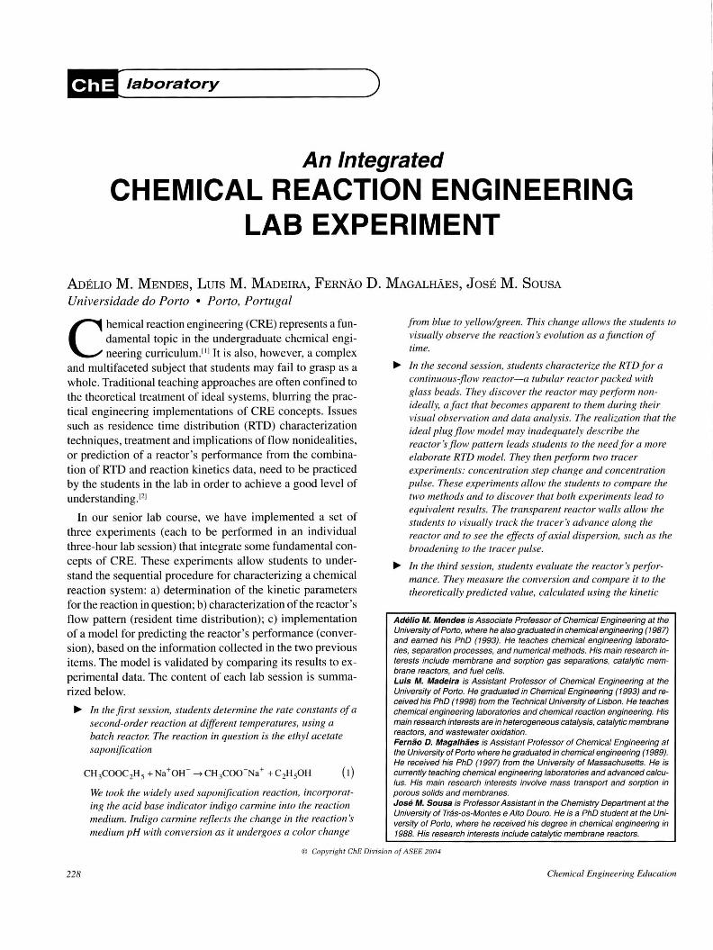
2) Flow pattern characterization in the packed-bed tubular reactor • Figure 3A shows the response of the packedbed reactor to a negative step change in terms of normalized concentrations, i.e., the so-called Danckwerts ' P curve. The slanted shape of the curve indicates that the flow dynamics
1.00
0.75
u"' u II 0.50 Z' ii:'
\ I
A
I \ \
0.25
0.00
\ I
\,__ I
0 200 400
t(s) 600 800
0.100
0.075
~o
.!!. 0.050
8'
0.025
0.000 0 200 400
t(s) 600
B
800
Figure 3. KC] normalized concentration data at the outlet of the packed-bed tubular reactor for (A) a negative step, and (BJ a pulse input. The lines represent the fittings obtained using Eqs. (4) and (9), respectively. The fitted parameters are shown in Table 1 .
TABLE 1 Fitted Parameters for the
Flow-Pattern Characterization Runs
Tracer Experime11t
Negative step input
Pulse input
Summer 2004
--Fitted Parameters --1(s) Pe Obj.Fem.
383.6 158.7 1.4 X J0·2
358.3 181.5 1.5 X 10·3
do not obey the ideal plug-flow pattern. Therefore, a more complete model must be used to describe the data. It is known that, for a semi-infinite axially dispersed plug-flow reactor, the residence time distribution (RTD) function is given by(6
·71
c;;- Pe(,-t) 2
E( t) = _\I_ ,re_ e- 4-,t-
2~ (3)
where -r is the space-time and Pe is the Peclet number. Students are informed that other equations can be found in the literature for the E(t) of a plug-flow reactor with axial dispersion, depending on the boundary conditions used. For small extents of dispersion (which is actually the case, as will be discussed below), however, the shape of the curve is insensitive to the boundary conditions imposed.141 The particular formulation adopted here has to do with the fact that an analytical solution exists and that this has a relatively simple form.
The outlet tracer concentration can be obtained from the E(t) by integration of Eq. (3), which provides the P(t) curve
t t Ne Pe(, - t)2
P( t) = ~ = I - f E( t )cit = I - f ~ e -4n dt co 2~
0 0
(4)
The parameters -r and Pe can be determined by fitting the model equation to the experimental data. This implies combining numerical integration and nonlinear fitting. Students can easily perform this task by using, for instance, the "Solver" add-in in Microsoft Excel. An initial estimate of the Peclet number for the fitting procedure can be obtained from available correlations, e.g., using the expression proposed by Chung and Wen 181 for a packed column with inert nonporous particles
0.2+0.0l{pu:P r48 L
Pe=----~-~-d p £
(s)
where Lis the length of the column, d is the average particle p
diameter, E is the bed porosity, u is the superficial velocity, and the other parameters refer to fluid properties. For this experiment, Eq. (5) leads to Pe= 202.9. A simpler estimation is based on the particle's Peclet number (Pe )
p
L Pe= PeP
dP (6)
In the current case, the Reynolds number is lower than 100, which implies that Pe varies in the range of 0.3 to l.0.191
p
Therefore, Eq. (6) yields an average value of 218 .8 for Pe (ranging between 101.0 and 336.7).
Table 1 shows the parameters obtained from the fitting . The objective function minimized was the sum of the squares of the residuals . Figure 3A clearly shows that the E(t) curve obtained with these parameters reproduces the experimental
231
data quite well.
Another very common tracer technique is the pulse input. If one can overcome the drawbacks associated with the implementation of a pulse injection, this technique represents a straightforward and less costly (less tracer is spent) way of obtaining the RTDJ 101 The concentration pulse can be mathematically formulated as
C/t) = CJH(t-0) - H(t-~t)]
where ~t is the duration of the perturbation and H(t) is the Heaviside function. The response of a continuous reactor to a pulse input in the feed stream is[7 1
C I I
C(t)=-= JE(t)dt- JE(t-~t)dt co O 0
(7)
where C(t) is the Danckwerts' C curve. For a sufficiently small pulse, i.e. , ~t • 0, Eq. (7) can be simplified to
M·E(t)
(s)
Thus, for an infinitesimal pulse, Eq. (8) will show a maximum at t = T. For a finite pulse, with length ~t, the maximum in the concentration will come out at t = T+~t/2. Extending this to the RTD function given by Eq. (3), the C curve becomes
Pe[,-{t+t.t /2) ]2
4,(t+t.t/2) (9)
Figure 3B shows the results of the pulse input tracer experiment. Equation (9) is fitted to the experimental data, yielding the parameters indicated in Table l. The good agreement between the experimental and theoretical curves in Figure 3B is particularly noteworthy, indicating once more that the reactor is well described by the axially dispersed plug flow model.
The otherwise colorless KCl tracer solution used in these experiments contains indigo carmine dye. This allows students to observe propagation of the concentration waves as they travel along the reactor. It is interesting to note that, for the pulse-input experiment, the tracer pulse is about 10 cm in length at the beginning of the run, but it noticeably spreads as it approaches the outlet, evidencing the existence of dispersion effects. Students find this experiment particularly interesting.
It is also interesting to actually look at the form of the E(t) functions obtained with the parameters computed from each tracer experiment. This is more conveniently done if one uses the normalized RTD function
232
~ Pe( l-8) 2
E(0)=tE(t)=--v_ree- - 48 -
2.Jne3 (IO)
where e = t!T . For the Pe and T values obtained from the two experiments, one obtains the plots shown in Figure 4. The similarity between the two curves is quite remarkable, considering that they were obtained by two distinct methods and under different operating conditions.
In a semi-infinite tubular reactor, the mean residence time, defined as
t = I tE( t )<it 0
or e=i= JeE(e)de t 0
is related to the space-time according tol61
or - I 0=1+
Pe (II)
From Eq. (11), as long as Pe is sufficiently large, as in the present case, t must tend to T, or 0 to 1. The RTD curves in Figure 4 show indeed that 0 is close to unity. This agreement indicates the absence of mixing problems in the reactor, such as short-circuiting or dead volume. The fact that Pe is relatively large traditionally implies that dispersion effects can be assumed as unimportant. That is also indicated by the almost-Gaussian shape of the RTD curves in Figure 4.141 Does this mean that axial dispersion can be neglected in this system (even though the presence of dispersion effects is evident from the experiments)? We ' ll get back to this question later.
3) Determination of conversion in the tubular reactor• Sodium hydroxide and ethyl acetate solutions are fed to the reactor until steady state is achieved, i.e. , a constant conductivity is measured at the reactor outlet. It is particularly interesting to observe the color gradient along the reactor-ye]-
Negative Step
3
$' ur2 -----
0.0 0.5 1.0
e 1.5 2.0
Figure 4. Normalized RTD function for the packed-bed tubular reactor based on the negative step and pulse
experiments (Pe values are shown in Table 1).
Chemical Engineering Education.
lowish at the entrance and blue at the exit. Students give particular attention to this fact and easily relate it to the concentration gradient in the reactor, which they've studied in the theoretical classes. At steady state, an average conductivity of 11.86 mS/cm is attained, corresponding to a sodium hydroxide conversion of 77.5 % (see Figure 5).
For a given RTD and reaction orders greater than unity, the total segregation model and the maximum mixedness model represent the upper and lower limits for conversion, respectively.1101 The total segregation model assumes that fluid elements having the same age (residence time) "travel together" in the reactor and do not mix with elements of different ages until exiting the reactor. Because no mass interchange occurs between fluid elements, each one acts as a batch reactor and the mean steady-state conversion ( X) in the real reactor is given by[IOI
= X = J Xbatch ( t )E( t )cit ( 12)
0
where xbalch(t) is given by Eq. (2) and the RTD function by Eq . (3), assuming that the axially dispersed plug-flow model properly describes the flow pattern in the packedbed reactor.
Using the two Peclet numbers obtained from the two flowpattern characterization experiments (step- and pulse-inlet perturbations) (see Table I) and the space-time corresponding to the present operating conditions, the total segregation model leads to a theoretical steady-state conversion of77.5 % (for Pe= 158.7) and 77.6% (for Pe= 181.5). Differences between the two results are minimal and both agree very well with the experimental result of 77.5%.
Axial dispersion is undoubtedly present in this system and, as shown before, it must be taken into account in order to accurately describe the flow pattern in the reactor. The in-
Figure 5. Sodium hydroxide conversion at the outlet of the tubular reactor. The lines were obtained using the total segregation model and the mass balance explained in Appendix B (with Pe= 158. 7 and -r = 348.3 s).
Summer 2004
quisitive engineer, however, might ask if the simpler ideal plug-flow model might not reasonably estimate the reactor 's conversion . Therefore, we ask the students to also compare the experimental steady-state conversion with the ideal plugflow model prediction (i.e., using Eq. (2) with the time t replaced by the space-time -r) . Interestingly, this model leads to a conversion of77 .7%, which is also remarkably close to the experimental result (77.5 %) ! This comes as no surprise if one considers the relatively low degree of axial dispersion present, which can be recognized a priori if one uses Eq. (6) for a first estimate of the Peclet number. The high L-to-d ratio (L/dP = 337) leads to a relatively high Pe. In conclusion~ the ideal plug flow model is not completely worthless. In this particular system, it is a straightforward and useful tool for estimating the reactor 's steady-state conversion. Students' attention is drawn to this issue, which may save time and effort in real-world engineering situations.
A more advanced topic that results from this experiment has to do with the prediction of the reactor 's start-up behavior, i.e. , the transient before the steady-state conversion is attained. The segregation model can also be used for this purpose, as long as the upper integration limit in Eq. (12) is set tot. The result obtained is shown in Figure 5. The agreement between the experimental and theoretical data is very good. The slight time lag between the curves is due to the difficulty in measuring the space-time rigorously. It must be noted that the ideal plug-flow model is not able to describe this behavior.
An alternative way to predict the conversion is based on the solution of the reactors' differential mass balance (see Appendix B). These computations involve solving a system of two partial differential equations (PDEs), which is far too advanced at an undergraduate level. It may be interesting to supply students with a software simulator that solves the balance equations, however, so they can analyze the results. The transient conversion computed from this approach is also shown in Figure 5 (see Appendix B for details). A steadystate conversion of 77 .2% is obtained (for any of the Peclet numbers mentioned above), which is once again in very good accordance with the experimental value. As expected, the steady-state conversion computed from the mass balance is lower than the one obtained from the segregation model-77 .5%-since the reaction order is greater than one. Differences are minimal, however, due to the high value of the Peclet number, i.e., low dispersion.
We frequently suggest that students perform an additional experiment, involving the removal of the static mixer at the reactor 's inlet, so that the two reactants enter through a simple "Y" connection. This causes improper mixing, leading to partial segregation and a decrease in the overall conversion. This fact is actually visible during the experiment: two differently colored symmetrical zones, each occupying about half of the reactor 's cross section, are perfectly visible along
233
its length . This can also be seen in the web site mentioned previously in this article. Students should ponder the fact that a simple flow-pattern characterization, such as the tracer experiments discussed here, is unable to detect this problem since fluid elements end up being mixed at the reactor outlet, before reaching the detector.
CONCLUDING REMARKS
The lab experiment described in this paper allows undergraduate students to integrate concepts taught in conventional chemical reaction engineering courses. In three independent lab sessions (each being about three hours long), they apply the fundamentals of: 1) determination of reaction rate constants in a batch reactor by applying the integral method; 2) characterization of the flow pattern (residence time distribution) in a tubular packed-bed reactor by trace experiments; 3) determination of the conversion in a continuous-flow reactor (both steady state and transient behavior). In the final written report, the information collected in each session is integrated to obtain a theoretical prediction of the conversion in the tubular reactor. The good agreement obtained between experimental and theoretical results helps students feel confident about their capabilities and improves their self-reliance regarding practical application of theoretical concepts.
The experiments are intrinsically safe and cost-moderate, while the reactants and products involved are nontoxic and environmentally nonaggressive or even biodegradable (at least considering the low concentration levels used) .
Using transparent reaction vessels and adding an acid-base indicator to the reactant and tracer solutions introduces a considerable pedagogical content. Some of the concepts involved are more easily understood and grasped by students, such as the progression of the reaction in the closed vessel, the existence of a concentration profile along the tubular reactor, and the more difficult notion of axial dispersion effects in a packed-bed reactor. The dispersion effects are more easily understood by students during the tracer experiments, particularly in the case of a concentration pulse, which is particularly fascinating for them.
ACKNOWLEDGMENTS
The authors gratefully acknowledge Ines Pantaleao and Nuno Barbosa, senior undergraduate students, for obtaining the experimental results and taking the photographs. We also wish to thank the Department of Chemical Engineering (Faculty of Engineering, University of Porto) for providing financial support for the set-up of the experiments.
NOMENCLATURE
234
C concentration of tracer, sodium hydroxide, or of ethyl acetate (mol·m·3)
C(t) Danckwerts' C curve, dimensionless dP diameter of the particles (m)
E(t) E(8)
E,
residence-time distribution function (s·') normalized RTD function, dimensionless activation energy (J ·mo)·')
H(t) Heaviside step function K0 initial conductivity in the calibration procedure
(mS cm·') K- final conductivity in the calibration procedure (mS cm·')
k reaction rate constant of the second-order reaction (m3moJ·1s·1)
k 0
L frequency factor (m3moJ·1s·') length of the column/reactor (m)
P(t) Danckwerts' P curve, dimensionless Pe Peclet number for the tubular reactor, dimensionless
Pep Peclet number for the particles, dimensionless t time (s)
t mean residence time (s) T temperature (K) u superficial velocity (m s·') V volume of reactor (m3)
v volumetric flow rate (m3s·') X conversion, dimensionless z length in the axial direction (m) Z dimensionless length in the axial direction
Subscripts EAc ethyl acetate
NaOH sodium hydroxide o entering or initial conditions
Greek Symbols ~t duration of the perturbation in a pulse input (s)
E bed porosity 8=th reduced time, dimensionless
µ fluid viscosity (N s m·2)
p fluid density (kg m·3)
T space-time (s)
REFERENCES I. Fogler, H.S. , "An Appetizing Structure of Chemical Reaction Engi
neering for Undergraduates," Chem. Eng. Ed. , 27, 110 ( 1993) 2. Shalabi, M., M. Al-Saleh, J . Beltramini, and D. Al-Harbi, "Current
Trends in Chemical Reaction Engineering Education," Chem. Eng. Ed., 30, 146 (1996)
3. Abu-Khalaf, A.M., "Mathematical Modeling of an Experimental Reaction System," Chem. Eng. Ed. , 28, 48 ( 1994)
4. Levenspiel, 0 ., Chemical Reaction Engineering, 3rd ed., John Wiley & Sons, New York, NY ( 1999)
5. Chen, N.H. , and R. Aris, "Determination of Arrhenius Constants by Linear and Nonlinear Fitting," A!ChE J. , 38,626 ( 1992)
6. Wen, C.Y., and L.T. Fan, Models for Flow Systems and Chemical Reactors, Marcel Dekker, Inc., New York, NY ( 1975)
7. Rodrigues , A.E., "Theory of Res idence Time Distributions," in Multiphase Chemical Reactors, A.E. Rodrigues, J.M. Calo, and N.H. Sweed, eds., NATO ASI Series, Sijthoff Noordhoff, No. 51 , Vol. I, 225 (1981 )
8. Chung, S.F., and C.Y. Wen, "Longitudinal Dispersion of Liquid Flowing Through Fixed and Fluidized Beds," A!ChE J. , 14, 857 (1968)
9. Ruthven, D. , Principles of Adsorption and Adsorption Processes, John Wiley & Sons, New York, NY ( 1984)
IO. Fogler, H.S., Elemellls of Chemical Reaction Engineering, 3rd ed., Prentice Hall , New Jersey ( 1999)
11 . Petzold, L.R. , and A.C. Hindmarsh, LSODA Computing and Mathematics Research Division, Lawrence Livermore National Laboratory, Livermore, CA ( 1997) 0
Chemical Engineering Education
APPENDIX A Calibration Method for NaOH Concentration
Measurement
During saponification (Eq. I) , one ion CH3COO· forms for each
OH ion consumed. These two species have very different mol ar conductivities, allowing for the reaction progress to be followed by conductometry. For that, students are asked to determine the molar conductivity of the involved ions in concentrations close to those employed in the runs. First, they must measure the conductivity (K0
)
of a sodium hydroxide solution having a concentration equal to the
start value used in the experiments ( C NaOHo ) (see Figure 6). K0 is
therefore associated with the presence of Na• and OH· ions, and for
C NaOHo =0. 1 M it has a value typically around 22.6 mS/cm. The
conductivity of the reaction product eventually obtained when all OH" is consumed (K- ), is therefore associated with the presence of only acetate and sodium ions and also has to be evaluated. An additional run is performed for this purpose, reacting a NaOH solution with 10-20% molar excess of ethyl acetate, to ensure total conversion, and measuring the final conductivity. For
M = C EAco IC aOHo = 1.25 and C NaOHo =0.1 M, K- is typically
around 7.3 mS/cm. The calibration line, which provides the sodium hydroxide concentration as a function of the conductivity of the reaction mixture, is therefore given by (see Figure 6)
K - K ~ CNaOH = CNaOH
o Ko - K~ ( 13)
Since the solutions are sufficiently diluted, linearity can be assumed.
APPENDIXB Mass Balance in the Axially-Dispersed Plug-Flow
Reactor
The tracer experiments have clearly shown that the continuousreactor is described by an axially dispersed plug-flow reactor. Thus, its performance can be predicted from the solu tion of the mass balance equations.
The system of two PDEs, each one describing the unsteady behavior of each reactant, is
~ a2c; _ ac; _ t ac ( ) kCNaOHC EAc =t-' i=NaOH,EAc
Pe az2 clZ cl t ( 14)
where Z=z/L is the dimensionless length in the axial direction. The boundary conditions, considering a semi-infinite reactor (open to diffusion at the inlet) are
C =C I I o
clC; = 0 az
at Z = 0 (i=NaOH, EAc) (15)
at Z = I (i = NaOH, EAc) (16)
The initial conditions are
CNaOH( t = 0 ) = CNaOH for '</Z 0
CEAc(t=O)=O for '</Z
Summer2004
(17)
(18)
E' <.>
K",---------------------=
20.0
Na++ CH3Coo· +CH3CHpH
Na+ + OH- + CH3COOCH2CH3
'.[ 10 .0 Na+ + OH. + CH3Coo· +
CH3CH20H + CH3COOCH2CH3 :.: K*
----- -- -- ----
0.0 ~-- --~----~----~----~ 0.00
c ,,•u01r
0.05
CNaOH (M)
0.10
C Nu0ll6
Figure 6. Calibration cu1ve for the method of analysisconductivity of the reaction mixture versus the
sodium hydroxide concentration.
A lab technician calibrates the conductivity electrode before classes so that students only need to normalize the conductivity data by the conductivity of the tracer solution used. When working with a relati vely broad concentration range, however, nonlinearity may be present and a correction factor must be considered. For that, students use data provided in the operator 's manual of the conductivity meter.
The spatial discretization along the axial coordinate was performed with 51 points, which was found to be quite satisfactory. A threepoint central difference scheme was employed for calculating the spatial derivatives. Routine LSODA1" 1 was used for time integration.
The outlet conversion obtained from the numerical solution of the mass balance equations is shown in Figure 5. This model predicts quite well the steady-state conversion. Regarding the transient behavior, one notices that the mean residence time estimated from the mass balance si mulated curve (338.8 s) is smaller than the experimental space-time (t = V/v = 348.3 s). indeed, this may be expected since the decreasing concentration profile in the reactor provides, in the mass-balance model , an additional driving force for the reactant's diffusion toward the outlet (and thus a lower mean residence time).
On the other hand, the total segregation model assumes no interaction between fluid elements of different ages and therefore the mean residence time is dependent on the RTD function alone, independently of the effect that the presence of chemical reaction might have. Thus, the mean residence time is practically equal to T , as previously explained. The slight shift of the experimental data with respect to this model is due to the error associated with the spacetime measurement.