Journal of Eliii’IER Journal of International Economics 39 (1995) 27-51 INTERRATfONAL ECONOMICS An integrated model of multinational flexibility and financial hedging Antonio S. Mello”7b’cv, John E. Parsonsd’*, Alexander J. Triantis” “Research and Statistics Department, Banco de Portugal, Rua Febo Moniz, 4, 1100 Lisbon, Portugal blJniversidade Catolica Portuguesa, Lisbon, Portugal ‘CEPR, London, UK ‘Graduate School of Business, Columbia University, New York, NY 10027, USA ‘School of Business, University of Wisconsin-Madison, Madison, WI 53706, USA Received March 1993, revised version received April 1994 Abstract We construct a model of a multinational firm with flexibility in sourcing its production and with the ability to use financial markets to hedge exchange rate risk. Agency costs generated by the firm’s capital structure create a link between the firm’s financial policy and its production decisions. The firm’s need for hedging is directly related to the degree of flexibility, and the production plan it chooses is a function of the hedging strategy it employs. Consequently, the firm’s ability to exploit its competitive position depends upon the degree to which its flexibility is matched by the construction of an appropriate hedging strategy. Key words: Production flexibility; Hedging; Currency risk JEL classification: F23; F31; G32 1. Introduction Exchange rate fluctuations pose several problems for a multinational firm. The economics literature has focused on the firm’s strategic response to the * Corresponding author. 0022-1996/95/$09.50 0 1995 Elsevier Science B.V. All rights reserved SSDI 0022-1996(94)01362-4
Transcript
Journal of
Eliii’IER Journal of International Economics 39 (1995) 27-51
INTERRATfONAL ECONOMICS
An integrated model of multinational flexibility and financial hedging
Antonio S. Mello”7b’cv, John E. Parsonsd’*, Alexander J. Triantis” “Research and Statistics Department, Banco de Portugal, Rua Febo Moniz, 4, 1100 Lisbon,
Portugal blJniversidade Catolica Portuguesa, Lisbon, Portugal
‘CEPR, London, UK ‘Graduate School of Business, Columbia University, New York, NY 10027, USA ‘School of Business, University of Wisconsin-Madison, Madison, WI 53706, USA
Received March 1993, revised version received April 1994
Abstract
We construct a model of a multinational firm with flexibility in sourcing its production and with the ability to use financial markets to hedge exchange rate risk. Agency costs generated by the firm’s capital structure create a link between the firm’s financial policy and its production decisions. The firm’s need for hedging is directly related to the degree of flexibility, and the production plan it chooses is a function of the hedging strategy it employs. Consequently, the firm’s ability to exploit its competitive position depends upon the degree to which its flexibility is matched by the construction of an appropriate hedging strategy.
Key words: Production flexibility; Hedging; Currency risk
JEL classification: F23; F31; G32
1. Introduction
Exchange rate fluctuations pose several problems for a multinational firm. The economics literature has focused on the firm’s strategic response to the
* Corresponding author.
0022-1996/95/$09.50 0 1995 Elsevier Science B.V. All rights reserved SSDI 0022-1996(94)01362-4
28 AS. Mello et al. I Journal of International Economics 39 (1995) 27-51
change in relative prices created by a shift in the exchange rate. For example, the firm may alter its pricing strategy (see the recent literature on pass-throughs including Baldwin and Krugman, 1989; Dixit, 1989a; and Marston, 1990) or may adjust its global production configuration (see, for example, De Meza and Van Der Ploeg, 1987, and Dixit, 1989a). The finance literature has focused on the design of securities and hedging operations with which the firm can lay off the foreign exchange risk. In most cases finance models take the firm’s exposure as given and ignore changes in the competitive position created by exchange rate movements and the firm’s strategic responses. Conversely, the economics literature usually ignores the role played by the firm’s liability structure in shaping its choice of strategy.
In this paper we construct an integrated model of real flexibility and financial hedging. We analyze a multinational firm with flexibility in sourcing its production and with the ability to use financial markets to hedge exchange rate risk. Hedging is used to reduce the agency costs generated by debt in the firm’s capital structure. The firm’s need for hedging is directly related to the degree of production flexibility, and the production plan it chooses is a function of the financial hedging strategy it employs. Conse- quently, the firm’s ability to exploit its competitive position depends upon the degree to which its flexibility is matched with an appropriate hedging strategy.
Following Dixit (1989b), we apply the state contingent model in continu- ous time now common in financial economics to evaluate the firm’s strategic options in the face of exchange rate uncertainty. We then incorporate the firm’s liability structure, solving for the firm’s optimal strategic decisions under alternative liability structures and hedging policies. We analyze the relationship between the firm’s production flexibility and the efficient hedging policy.
In our model capital markets are internationally integrated and all cash flows contingent upon the exchange rate can be priced with a dynamic replicating portfolio of riskless bonds denominated in each of the two currencies. All exchange risk therefore has a unique price and the firm cannot earn any risk-sharing benefits from financial hedging. The Modig- liani-Miller theorem obtains in the sense that a given operating policy yields a determinate value of the firm independent of any financial hedging. Hedging, however, will affect the firm’s choice of operating policy and thereby the firm’s value.
The corporate finance literature hypothesizes a variety of reasons why a firm’s liability structure might affect its strategic decisions. In an inter- national context each of these reasons can explain how a firm may benefit by hedging foreign exchange exposure. For concreteness we focus upon the agency problems created by outstanding debt which were origi- nally analyzed by Stiglitz and Weiss (1981) and by Myers (1977). The
A.S. Mello et al. I Journal of International Economics 39 (1995) 27-51 29
multinational firm’s decision to finance its operations with debt denomi- nated in some combination of two available currencies shapes its choice of strategy regarding when to shift production from one country to the other in the face of exchange rate movements. Importantly, our model enables us to determine the extent to which issuing a given profile of debt distorts the firm’s international production and sourcing decision. Implementing the right foreign exchange hedge when issuing the debt reduces the distortion, encouraging more efficient decisions and thereby raising the firm’s value.
Since the benefit of hedging is directly related to the optimality of a given production strategy, it is obviously important to evaluate the hedge using a model that explicitly incorporates the firm’s real flexibility in shifting production between countries. This model fills an important gap in the literature on foreign exchange hedging. It has been widely recognized that the firm’s international competitive position affects its actual exposure to exchange rate movements (see Hodder, 1982; Cornell and Shapiro, 1983; and Adler and Dumas, 1983). Standard international finance textbooks focus attention on the relationship between multinational competitive strategies and exchange risk, without, however, being able to provide any quantitative tools with which to analyze or measure the phenomenon (see, for example, Shapiro, 1988, pp. 321-349). The dynamic effects of a firm’s strategic decisions make the task of valuing the firm and measuring foreign exchange exposure extremely difficult. Simple models for minimizing the variance of firm value cannot properly reflect the complicated impact of the firm’s contingent strategy. Our model allows one to precisely measure the firm’s exposure at any point in time, fully accounting for the firm’s ability to respond strategically to exchange rate movements. The model permits us to measure the impact of a particular hedging strategy.
An integrated model also enables us to relate the literature on why firms hedge with that on how to hedge. Many of the models used to explain why firms hedge have been constructed in a stylized manner in order that the key forces bearing on the motive for hedging are apparent. These models have no place for the traditional tools used to measure foreign exchange exposure nor for the familiar contingent claims mechanics used to construct a given hedge or to value specific securities. The literature on the mechanics of hedging, on the other hand, establishes a number of alternative means by which to repackage exchange risk while abstracting from the motivation for hedging. The model presented here resolves this dichotomy.
The paper is organized as follows. In Section 2 we model a firm with multinational production flexibility. In Section 3 we introduce the firm’s liability structure and analyze the benefits of financial hedging. In Section 4 we analyze the relationship between financial hedging and production flexibility. Section 5 concludes the paper.
30 AS, Mello et al. I Journal of International Economics 39 (1995, 27-51
2. The model of a multinational firm
Consider a multinational firm with an infinite horizon and one unit of production capacity in both the United States and Japan. The firm can sell one unit of output in the United States. The price of the output, p, is denominated in dollars. Unit production costs in the United States, cu, are denominated in dollars. Unit production costs in Japan, cJ, are denominated in yen, and are translated into dollars at the current exchange rate s. The exchange rate is random.* Since combined capacity is greater than the size of the market the firm will generally source its production in the country where costs are lowest, depending upon the prevailing exchange rate. In switching production from one country to the other, however, the firm incurs a fixed and non-recoverable cost, k, denominated in dollars.’ Because of this fixed cost, the exchange rate at which the firm will move production from the United States to Japan, suJ, is lower than the exchange rate at which there is parity in production costs: suJ c fpf where sP = c,/c,. The converse holds for moving from Japan to the United States, so that suJ G s,, s sJu. When the exchange rate lies within the bounds of the two switching points, s E 1s uJ, sJu), the firm may be producing either in the United States or in Japan, depending upon the past history of exchange rate movements. This region of hysteresis has been identified in earlier models of a similar nature by Dixit (1989a, b).
To maintain the generality of the model we recognize as well that the firm may exit the industry entirely. The exchange rates at which it would exit when it is currently operating in the United States and Japan are denoted sou and &,J, respectively. Of the four exchange rates, suJ, sJu, sou and so,, one is always redundant. For example, if sJu <so,, then, in the face of rising exchange rates, the firm will switch production from Japan to the United States before the exchange rate ever reaches soJ, the critical rate for exit while producing in Japan: hence the firm will only exit the industry from the United States and not from Japan.3 For brevity of exposition we focus on
’ The model developed here can also include a random output price. In order to focus on exchange risk and to make the solution analytically tractable we present the case of the single random variable. Output prices of manufacturing industries are much less vofatile than exchange rates, so this case is of some practical interest. We briefly discuss the two-variable case at the end of the paper.
‘The model can be easily generafized to admit different costs of switching to and from the United States and denominated in either or both currencies.
3 Note that when the exchange rate exceeds slu, the firm’s current cash flow is independent of small variations in the exchange rate. However, the firm’s value continues to depend upon the exchange rate through expectations about future cash flows. For example, the exchange rate might fall below suJ, in which case the firm would switch its production back to Japan and its cash flow would once again fluctuate with the exchange rate. The probability of this event occurring within any given horizon is conditioned by the current exchange rate, and therefore so too is the firm’s value and its exit decision.
A.S. Mello et al. I Journal of International Economics 39 (1995) 27-51 31
this case, with suJ c sJu ssOu, allowing for the possibility that sOu is arbitrarily large.
A triple of critical exchange rates, 4 = (suJ, sJu, so”), constitutes an operating policy for the firm. The value of the firm is a function of the operating policy chosen by the management, and of the prevailing exchange rate. Due to the hysteresis, the firm’s value will also depend upon the current location of production. We denote by vJ(s; 4) and vu@; 4) the dollar denominated value of the firm when currently producing in Japan and when producing in the United States, respectively.
Deriving an expression for the firm value can be problematic. The firm’s flexibility truncates or otherwise skews the distribution of the firm’s profits and causes this distribution to become dependent on the current location of production and on the exchange rate. Therefore, a single risk-adjusted discount factor cannot be used to compute the firm value. An alternative valuation tool is the state contingent model in continuous time. State contingent prices can be implicitly derived using techniques developed in Black and Scholes (1973) and Merton (1973). Let the exchange rate, s, follow the exogenous stochastic process ds = psdt + asdz, where p is the instantaneous drift in the spot exchange rate, m is its instantaneous standard deviation, and dz is the increment to a standard Gauss-Wiener process, with zero mean and variance dt. Any pattern of future cash flows contingent on the exchange rate can be replicated as a dynamically rebalanced portfolio composed of two bonds. The first bond pays a riskless dollar interest rate, ru, and the second bond pays a riskless yen interest rate, r,. The dollar return on the yen denominated bond is a function of the stochastic exchange rate and is therefore risky. Hence, different combinations of the two assets generate different patterns of dollar denominated risk and return over any interval.
It is possible to determine the firm’s value by constructing a portfolio of the two bonds that matches or replicates the risk and dollar return of the firm’s operations. The return earned by the firm is the sum of its cash flow and instantaneous change in firm value. Assume the firm is currently operating in Japan. The firm’s instantaneous cash flow is (p - sc,)dt. The instantaneous dollar change in firm value is given by dv = (1/2)~:,(&)~ + vjd.s, where v,’ and vf, denote the first and second partial derivatives of the firm’s value with respect to s, respectively. This follows from Ito’s Lemma. Combining these two components of return, the total dollar return earned by the firm is
(p - sc,)dt + (1/2)~j,(ds)~ + v&.
The replicating portfolio of dollar and yen denominated riskless assets with current value vJ and the same risk as the firm is constructed by lending vf yen and v’ - vf, dollars. The instantaneous dollar return on the yen and
32 A.S. Mello et al. I Journal of International Economics 39 (1995) 27-51
dollar positions are vLd.s + svfr,dt and [v’ - vis]r,dt, respectively. The total return on this portfolio must be equal to the total return earned by the firm, since both the risk and the initial investments are equal. Rearranging the terms in the resulting equality yields the following differential equation which vJ must satisfy at every exchange rate, s:
(1/2)v;$s* + v;(r” - T’)S - ruvJ +p -SC’ = 0. (1)
Using a similar derivation, but recognizing that the instantaneous cash flow earned when the firm is operating in the United States is equal to (p - cJ, the function describing the value of the firm operating in the United States, V “, must satisfy the differential equation:
(1/2)4r2s2 + v,u(ru - T’)S - ruvu +p -cu = 0. (2)
In addition to these differential equations, the two value functions must satisfy an identity at each of the critical exchange rates. Suppose the exchange rate is suJ, so that the firm operating in the United States is about to spend k dollars to switch production to Japan. The firm already operating in Japan has the same value, plus the k dollars not spent moving to Japan:
V&J; d’) = vu(s”J; d’) + k . (3)
Conversely, the firm already operating in the United States when the exchange rate is sJu, is worth a premium of k dollars over the firm operating in Japan but about to move production to the United States:
v”(sJ”; d’) = vJ(sJ”; 4) + k . (4)
When the firm is about to exit the industry, its value must be equal to the exogenously specified liquidation value, z, which we allow to be a function of the exchange rate:
v”(%“~ 4) = 4%“) * (5)
Using Eqs. (3)-(5) as boundary conditions for the differential equations (1) and (2), it is possible to derive explicit solutions for v’ and v” which take the form:
(6) vJ(s,d+= (t-7) +&Jlsyl,
v”wb)= (f-3 +P”ulsy~+P”u2syz, (7)
A.S. Mello et al. I Journal of International Economics 39 (1995) 27-51 33
where y1 > 1 and y2 < 0 are constants and where pyI1, pVul and pvu2 are functions of the specified operating policy, 4. Expressions for these terms are given in the appendix.
These equations have a straightforward interpretation. Consider first Eq. (6), the value of the firm when operating in Japan. The term in parentheses is the current value of a perpetual stream of cash flows from production based in Japan given the current exchange rate, s. A rise in the exchange rate makes production in Japan more expensive and lowers the value of the firm. The firm with multinational flexibility can escape these rising variable costs by moving production to the United States after paying the switching cost, k. Should the exchange rate fall again the firm can shift production back to Japan. The value of this flexibility is represented in Eq. (6) by the additional term, pVJ1syl.
The dotted line in Fig. 1 plots the value of the term in parentheses from Eq. (6) at different exchange rates. The left-most solid line in Fig. 1, intercepting the vertical axis at p/r”, plots the function vJ at different exchange rates. The distance from this solid line to the dashed line is the value of flexibility, /3,,,rsy1. In Eq. (7), the term in parentheses is the current value of a perpetual stream of cash flows from production based in the United States. The first additional term, /3VuIsy1, is the value of the firm’s flexibility to switch production to Japan and back. The second additional term, Pvu2syz, is the value of the total expected future savings from closing the firm in the face of rising exchange rates instead of continuing operations at a loss. Whereas the first additional term is an option to exit a location while staying in the industry, the second is an option to exit the industry altogether.
The value equations (6) and (7) hold for any arbitrary production policy. The policy that maximizes firm value is denoted +FB = (sR, SF:, $E). The maximum firm value and this first-best policy must be derived simul- taneously, using Eqs. (l)-(5) and optimality conditions developed in Merton (1973). The first of these optimality conditions is
vi. FB(S$ 4”“) = $3 FB(SR; +FB) . (8)
To understand this condition, suppose that at the switching point SE, a marginal increase in the exchange rate caused firm value to decline less in Japan than in the United States, so that Eq. (8) is violated. Using Eq. (3) one can show that at an exchange rate marginally greater than the hypothesized first best, S > SE, the firm would have a higher value by switchin
63 production from the United States to Japan and so the hypoth-
esized sur could not be the optimal switching point. Two similar optimality conditions obtain at the other two critical exchange rates:
34 A.S. Mello et al. / Journal of International Economics 39 (1995) 27-51
Fig. 1. The value of a firm with operating flexibility as a function of the exchange rate. The value of the firm when operating in Japan, ~‘(3; c$), and when operating in the United States, vu@; r$), are graphed for different exchange rates. The dotted line graphs the present value of a perpetual stream of cash flows from production based in Japan for different exchange rates. The difference from the dashed line to the solid line, ~‘(3; +), represents the value of the real option to switch production from Japan to the United States, and back. The three critical exchange rates defining the firm’s operating policy, I$, are s,,, s,,, and s,,,,, and at these exchange rates the value functions ~‘(8; 4) and v”(s; 4) satisfy boundary conditions (3) (4) and (5) respectively.
Vf’FB(S;$ $I”“) = lyFB(sJFUB; 4”“) ) (9)
Expressions for the critical exchange rates in the first-best operating policy are given in Eqs. (A4)-(A6) of the appendix.
It should be noted here that although we chose to value all claims in US dollars, the analysis would be equivalent if the yen had been chosen as the numeraire. The yen value of the firm, its equity, or any of its liabilities, are
A.S. Mello et al. I Journal of International Economics 39 (1995) 27-51 35
always the product of the dollar value and the inverse of the current exchange rate. Policies chosen to maximize the dollar value of any liability therefore always maximize the yen value as well. This highlights that the benefits of hedging to be discussed in Section 3 do not depend upon international risk-sharing issues. Capital markets in this model are interna- tionally integrated. Neither the firm nor its investors have any special nationality.
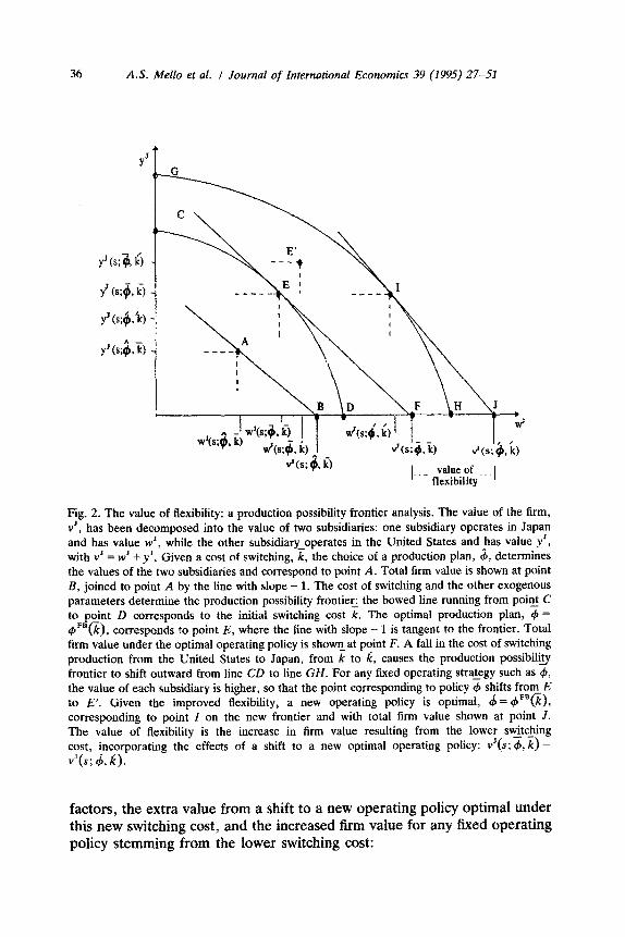
For purposes of our later discussion it is useful to analyze the value of flexibility in a production possibility frontier analysis of the firm as displayed in Fig. 2. The multinational firm can be decomposed into two subsidiaries, one that receives cash flows only when the firm is operating in Japan, and one that receives cash flows only when the firm is operating in the United States. The value of the firm, vJ, is equal to the sum of the values of the Japanese and the US subsidiaries, wJ and yJ, which are plotted on the horizontal and vertical axes, respectively. The set of equations used to calculate wJ and yJ are similar to those used to calculate the value of the firm as a whole, and are given in the appendix.
Given a switching cost, k, the choice of an arbitrary operating policy, 3, determines a point in the positive quadrant, for example, point A in Fig. 2. Total firm value under 3 is the simple sum v’(s; 4, k) = wJ(s; 4, k) + yJ(s; 4, ‘is), and is shown on the horizontal axis at point B, connected to point A by the line with slope - 1. The solid bowed line running from point C to point D is the production possibility frontier: points along this frontier correspond to different operating policies which maximize the value of one subsidiary while fixing the value of the other subsidiary. The operating policy that maximizes firm value given this switching cost, 4 = +““(%), corresponds to point E where the market value line is tangent to the -- frontier. Firm value under this first-best operating policy, vJ(s; 4, k), is shown at point F.
A fall in the cost of switching production from k to k causes the value of both subsidiaries to increase so that the former first-best operating policy, 3, now corresponds to point E’. The firm’s entire frontier is shifted outward, from CD to GH, so that a new operating policy, 4 = 4’“(k), corresponding to point I maximizes firm value. The first-best value of the firm increases to vJ(s; 4, k) at point J. This increase is the measure of the value of extra flexibility:
AvJIAk = vJ(s; 4”“(k), k) - vJ(s; 4’“@), k),
where decreasing the switching cost (Ak = k -k CO) corresponds to an increase in flexibility. It is straightforward to decompose this into two
36 A.S. Mello et al. I Journal of InternationaI Economics 39 (1995) 27-51
Fig. 2. The value of flexibility: a production possibility frontier analysis. The value of the firm, v’, has been decomposed into the value of two subsidiaries: one subsidiary operates in Japan and has value w’, while the other subsidiary-operates in the United States and has value y’, with v’ = w’ f y’. Given a cost of switching, k, the choice of a production plan, 4, determines the values of the two subsidiaries and correspond to point A. Total firm value is shown at point B, joined to point A by the line with slope - 1. The cost of switching and the other exogenous parameters determine the production possibility frontiec the bowed line running from point C to p$nt D corresponds to the initial switching cost k. The optimal production plan, d, = QIF8(k), corresponds to point E, where the line with slope - 1 is tangent to the frontier. Total firm value under the optimal operating policy is showEat point F. A fall in the cost of switching production from the United States to Japan, from k to k, causes the production possibilig frontier to shift outward from line CD to line CH. For any fixed operating strategy such as #, the value of each subsidiary is higher, so that the point corres~n~ng to policy d, shifts from E to E’. Given the improved flexibility, a new operating policy is optimal, (f = (B”“(@, corresponding to point I on the new frontier and with total firm value shown at point J. The value of flexibility is the increase in firm value resulting from the lower switching cost, incorporating the effects of a shift to a new optimal operating policy: v’(s; #, k) - vys; 4, I;).
factors, the extra value from a shift to a new operating poIicy optimal under this new switching cost, and the increased firm value for any fixed operating policy stemming from the lower switching cost:
A.S. MeNo et al. I Journal of International Economics 39 (1995) 27-51 37
AvJIAk = [vJ(.s; 4”“(k), k) - vJ(s; $~““o;), k)]
+ [vJ(s; (b”“@), /q - vJ(s; f#JFB@), k)].
3. The benefits of financial hedging
We now incorporate the firm’s liability structure into our model of the firm’s choice of production plan and valuation. Agency costs associated with debt, in particular those originally analyzed by Stiglitz and Weiss (1981) and by Myers (1977), raise the possibility that hedging foreign exchange risk can increase firm value. Issuing debt impacts the firm’s value through the incentives it creates for management to choose a different production plan. When there are multiple claims against the firm’s cash flows, we assume that management chooses the operating policy that maximizes the value of equity. The levered equity owners’ optimal operating policy, +*, is usually different from the first-best policy, so that the actual value of the firm is usually strictly less than the first-best value: vJ(s; $*) < vJ(s; 4’“). The difference is the agency cost created by the outstanding liabilities: vJ(s; 4”“) - vJ(s; +*). Implementing a hedge simultaneously with issuing the debt changes the firm’s effective liability structure and therefore the equity owners’ choice of a production plan. An efficient hedge is one that results in the firm implementing the first-best operating policy.
3.1. Valuing the jirm with multiple liabilities
The equity owner’s optimal choice of a production plan is determined together with the value of the equity. Denote by eJ and e” the value of the equity depending upon the location of the firm’s current production. The function describing the value of equity is derived in a fashion comparable with the earlier derivation of firm value, with two modifications.
First, cash flows to debt and to any hedge contracts are deducted from (or added to) the firm’s cash flow to yield the cash flow to equity. Denote by O(S) the aggregate dollar denominated senior claims to the firm’s cash flow. This functional form allows as one possibility that some of the outstanding debt is denominated in yen and therefore that the aggregate annual dollar cash flow on the liabilities fluctuates with the exchange rate. For simplicity we assume that senior claims are perpetuities in whatever currency they are denominated. Under this restriction the model has an analytic solution. Senior claims with a time-dependent cash flow can be incorporated, but the solutions must be derived with numerical estimation techniques. The levered equity owners’ cash flow is then given as p - scJ - 6(s) when the firm is
38 A.S. Mello et al. I Journal of International Economics 39 (1995) 27-51
operating in Japan and p - cu - O(s) when producing from the United States.
Second, equity owners have the option to default on their obligations, and they will do so whenever the value of the outstanding liability is greater than the value of the cash flows expected from the firm at the given exchange rate. We denote this critical exchange rate s&. In general the equity owners will default in the face of rising exchange rates at some point prior to the efficient exit point, s& < si:. Upon default the equity is worthless, and so the following boundary condition holds:
e”(s&; l#l*) = 0. (11)
The complete program for valuing the equity is given in the appendix. The firm’s value under the equity owners’ optimal operating policy must
be calculated using Eqs. (l)-(4) and accounting for the consequences of default. We assume that upon default the firm is reorganized and sub- sequently operated according to the first-best operating policy. However, we allow that there may be deadweight costs associated with bankruptcy. Consequently the value of the firm upon default may be less than the first-best value:
V”(S& 4*) = “v”(sd”; 4”“), a E [O, 11. (12)
The exogenous variable (Y parameterizes the magnitude of the deadweight bankruptcy costs, with a decrease in (Y corresponding to an increase in these costs. If a = 1, then there are no deadweight costs to bankruptcy. Condition (12) is analogous to condition (5) in the program for calculating the first-best value of the firm.
All of the other claims against the firm can be valued in a similar fashion, taking the firm’s production plan as given. A program for valuing the yen and dollar denominated debt of the firm is given in the appendix.
3.2. Debt, operating policy, and the benefits of hedging
A firm issuing debt can simultaneously hedge its exchange rate exposure using forward contracts written on the exchange rate. Packages of forward contracts on the exchange rate covering a range of years are commonly negotiated in the form of currency swaps. Following the usual convention employed in currency swaps, the firm is said to have sold one contract if it agrees to pay at future time, t, 1 yen with uncertain dollar value, sI, in exchange for receiving at that future time a dollar denominated certain payment, f,. Without loss of generality we assume that the hxed payment is constant for all time periods covered by the swap and so drop the subscript on f. Under our assumption of an infinite time horizon for the firm’s
A.S. Mello et al. I Journal of International Economics 39 (1995) 27-51 39
production capacity and our assumption that all debt issues are perpetuities, it is possible to restrict our attention to currency swaps composed of forward contracts maturing at every point in time t E (0, a). We are interested in the size of the hedge, 12, which is the number of forward contracts in the swap sold by the firm. Denote by $(s, f; c$*) the market value of this swapP
Arranging a currency swap at the time the firm issues debt reshapes the incentives of the equity owners as they choose the critical exchange rates at which to shift production from one country to the other or to abandon the market entirely. Suppose, for example, that the firm issues debt obligations denominated both in dollars and in yen, with annual payments 6% and 6 y, so that the total dollar denominated cash flow on liabilities is 8 (s) = S $ + s6 ’ . Given this debt structure, the manager will choose a particular operating policy, 4*(e). If the firm hedges using a swap with n packages of forward contracts with price f, the total dollar denominated cash flow to liabilities at each t E (0,~) becomes z(s) = S $ + s6 ’ + n(s -f). Under this new liability structure the manager chooses a different production plan, +*@). A swap contract efficiently hedges the debt issue if it gives the equity owners an incentive to choose the first-best production plan, thereby increasing the firm’s value.
There are two distinct sources for the increase in firm value. First, hedging shifts management’s choice of critical exchange rates at which to shift production back and forth between the two countries, s,” and suJ. The choice of a location for production can be compared with the general choice of alternative projects with different risk and return. Outstanding debt distorts management’s valuation of the risks involved-see Stiglitz and Weiss (1981) and Myers (1977). In our model this means that management chooses critical exchange rates for shifting
FE reduction between the two countries that
differ from the first best, sJ*” #s,” and s& # sz, and an efficient hedge is one that recreates an identity between the levered equity owners’ optimal policy and the first-best policy. Second, an efficient hedge decreases the probability that equity owners default, reducing the deadweight costs incurred in bankruptcy. Which of these two sources of hedging benefits is more important depends upon the parameterization of the problem. The
4The cash flows from the swap can be replicated by a dynamically-rebalanced portfolio of dollar and yen bonds, and thus its value can be found with equations similar to those used to value the firm’s outstanding debt and described in the appendix. Often the convention is to set the forward price, f, such that the market value of the swap is equal to zero at the time it is negotiated, t = 0. This is similar to the convention used with forward contracts which yields the well-known pricing equation f, = soexp[( ru - r,)t]. Similarly, in our context, if the entire package of forward contracts were free of credit risk, the forward price, f, which yields a zero market value for the package, has the simple form f =so(ru/r,). Of course, this covered interest parity formula assumes that the contract is default-free. In our model, we value and price the swap contract incorporating the possibility that the firm may default.
40 AS. Mello et al. I Journal of International Economics 39 (1995) 27-51
value of hedging is also contingent upon the current exchange rate in relation to the critical rates describing the production plan. If deadweight costs of bankruptcy are significant, then the value of hedging will be greater when the exchange rate has pushed management close to default. Similarly, if the exchange rate is close to one of the critical exchange rates at which management plans to switch production from one country to the other, then the benefit from improving this decision will be greater.
The gains from hedging are illustrated with a numerical example de- scribed in Table 1. Two firms with the same operating flexibility and with identical debt outstanding are contrasted. One firm has no hedge in place, while the second firm has set up an efficient hedge. Using the model described above and the equations specified in the appendix, we calculated the production plan chosen by both managements as well as the resulting firm, equity, and debt values, with and without hedging. The firm with no hedge defaults, while the firm that hedges efficiently implements the first- best exit policy, avoiding default entirely. Given the parameters specified in Table 1, the efficient hedge consists of selling 28 packages of forward contracts on the yen. The value of the hedge (not to be confused with the value of the package of forward contracts) is the increased firm value resulting from the improved production plan5
The benefit from hedging can be analyzed using the production possibility frontier diagram employed earlier and displayed in Fig. 3. The exogenous
Table 1 The value of financial hedging By introducing an appropriate hedging package, the value of equity increases in the levered firm. This occurs because the critical exchange rate at which the firm defaults on its debt increases and so the expected value of the deadweight costs of bankruptcy fall. The value of the hedge is equal to the rise in equity value. We examine two firms, one without a hedge in place, and the other with an optimal hedging package. Common parameers for the two firms are p = 10.2, cus = $10, c, = YlOOO, rus = 2%, r, = 2%, a,,, = lo%, (Y = 0 and k = $50. The current exchange rate is s = 0.01 $/Y. Both firms have U.S. debt outstanding with continuous coupon rate of $1 per annum.
Firm value, Debt value, Equity value, Number of Operating u”(s; 9*) buts; 4*) e”(s; $*I hedging policy,
‘While our model enables us to value the firm with any arbitrary hedge, we only report results for a firm with no hedge and for a firm with the efficient hedge.
A.S. Mello et al. I Journal of International Economics 39 (1995) 27-51 41
1 value of an efficent hedge -I
Fig. 3. The value of hedging: a production possibility frontier analysis. The exogenous parameters of the problem, including the costs of switching production between the two countries, determine the location of the production possibilitylrontier shown as the bowed line connecting points C and D. The first-best operating policy, I$ = +FB, corresponds to point E and to the aggregate firm value at point F. Financial hedging cannot shift this frontier outward and cannot increase the maximum feasible firm value above v’(s;G). However, a firm with outstanding debt and without a hedge will choose an operating policy, 4, associated with an interior point such as K. Implementing an efficient hedge induces management to choose the first-best operating policy and move the firm mpoint E. The value of the efficient hedge is the difference between the two firm values: v’(s; 4) - v’(s; 4).
parameters of the problem, including the costs of switching production between the two countries, determine the frontier CD. The first-best operating policy corresponds to point E. A levered firm without a hedge chooses an operating policy interior to the production possibility frontier and corresponding to point K. An efficient hedge gives the equity owners of the levered firm an incentive to choose the first-best operating policy and so moves the firm to the frontier at point E.
Some final comments are in order about the nature of the hedges analyzed here. First, it is important to notice that the entire package of forward contracts composing a hedge in our model is negotiated at time t = 0. The equity owners benefit from negotiating the swap contract simultaneously with the issuance of debt since the value of the debt is determined under an
42 A.S. Mello et al. I Journal of International Economics 39 (1995) 27-51
assumption about the operating policy to be followed by the firm: with an efficient hedge in place the creditors require a smaller nominal obligation in exchange for the same capital contribution.
The same results cannot be achieved using short-term futures contracts sold on an exchange and continuously rebalanced because the agency problems created by the outstanding debt undermine the equity owners’ incentive to rebalance the hedge through time. This is the familiar time- inconsistency problem for dynamic games. Hence the model makes a critical distinction between long- and short-term hedging contracts and policies.
Second, the questions arise: Would it be in the interest of the equity owners to undo its hedge through subsequent trades in short-term futures contracts? Must the firm commit not to undo its hedge? Do we require that the firm be prohibited from subsequent trading in short term futures or other derivative contracts? The answer to these questions is no. It will not be in the interest of the equity holders to later undo the hedge negotiated at the outset. The same covenants that would be included in the debt absent a swap also protect the debt with a swap: i.e. that (i) any additional debt or swap or futures contracts must be junior to the original debt in the sense that upon default the original debt is paid first, and (ii) the equity cannot pay out the proceeds of the new contracts as dividends.
Third, whenever both the dollar and the yen denominated cash flows on the original bonds cum efficent hedge are positive, the hedge can be reinterpreted as an exchange of one pair of bonds for another pair with denomination weighted more or less to the dollar or the yen. The model presented here is then a means to determine the optimal currency denomi- nation of the debt the firm issues. Different currency denominations imply different agency costs. The optimal currency denomination minimizes the agency costs for any given market value of debt issued.
4. The interaction between operating flexibility and financial hedging
The model presented above enables us to determine an optimal hedging policy for a firm with multinational flexibility. This is a significant improve- ment over existing models. Most analyses of the firm’s exposure are necessarily myopic, taking the existing production framework as static, and simply measuring the correlation between the exchange rate and either cash flows or firm values as if this relationship were stable. These myopic solutions give biased recommendations about the appropriate size of a hedge: a flexible firm currently operating in the United States would appear to face no exchange risk, while the same firm currently operating in Japan would appear to face significant exchange risk. The failings of these myopic tools have been well documented, and the need to incorporate the firm’s
A.S. Mello et al. I Journal of International Economics 39 (1995) 27-51 43
ability to alter its sourcing and sales decisions in the face of exchange rate risk is commonly understood (see, for example, Cornell and Shapiro, 1983). However, the dynamic and contingent character of the firm’s sourcing decisions, and the problems of valuing the firm under these circumstances, make it difficult to include these factors in traditional exchange risk models. Our paper integrates production flexibility and valuation, making possible the correct measurement of exchange exposure and the construction of efficient hedging strategies.
We now examine the relationship between flexibility and hedging, using some simple numerical examples that illustrate how the firm’s need for hedging is directly related to the degree of flexibility, and how the production plan it chooses is a function of the hedging strategy it employs. In Table 2 we report the size of the efficient hedge-the number of hedging packages required to induce the first-best operating policy-as a function of
Table 2 Interactions between flexibility and hedging: Optimal hedge packages Optimal hedge packages for firms with comparable debt structures and different degrees of flexibility are contrasted. In panel A the debt packages are identical in nominal terms. In panel B the firm leverage ratios are equal. Common exogenous parameters for the firms are p = $10.2, ens =$lO, c, = YlOoO, rus =2%, r, =2%, css;+, = 10%. and cr = 0. The current exchange rate is 0.01 $/U.
Panel A: the optimal hedge packages for two firms with identical nominal debt obligations and differing switching costs are contrasted. The switching cost for the firm with high flexibility is k = $0, and the cost for the firm with low flexibility is k = $50. Both firms start off with U.S. debt with continuous coupon rate of $1 per annum. The value of debt differs due to the higher probability of default in the firm with less flexibility.
Unhedged Debt Equity Hedged firm value, value, firm value b”(s; &*) e”(s; &*) value
Number of Value of hedging hedging contracts vFB --u*
Panel B: The optimal hedge packages for two firms with identical leverage ratios and differing switching costs are contrated. Both firms have debt/value ratio of 29% when efficiency hedged. The firm with high flexibility has coupon rate $0.8 p.a. and the firm with low flexibility has coupon rate $0.534 p.a.
Unhedged Debt Equity Hedged Number of Value of firm value, value, firm hedging hedging value b”(s; 4*) e”(s: 4”) value contracts vFB - v* u”(s; 9*) u”(s; 4’“) n
44 AS. Mello et al. / Journal of International Economics 39 (1995) 27-51
the firm’s flexibility. Also shown is the change in firm value, vFB - v* . We find, for example, in panel A, that the size of the efficient hedge increases by 7.05, from n = 21.00 to y1= 28.05, as the degree of flexibility decreases from k = 0 to k = 50. We find that efficient hedging increases the value of a firm with low flexibility by 6 percent, while for a firm with high flexibility the efficient hedge increases value by 2 percent.
The fact that both production flexibility and financial hedging increase firm value in the face of exchange rate risk suggests that ~exibility and hedging are substitutes-alternative ways of achieving the same objective. Intuition would suggest that a relatively more flexible firm-one that has a greater ability to source its production abroad in response to sharp movements in the exchange rate-has less need to hedge its foreign currency profits. We can check this intuition against results from our model. The results discussed above for panel A seem to be consistent with this intuition. Improved flexibility means, by definition, that the contingent cost structure of the firm is lower and so firm value increases. The increase in value makes default less likely and therefore lowers the expected deadweight costs of bankruptcy, so that the value of hedging declines.
However, consider a second comparison contradicting this intuition. Suppose we identify two firms, comparable in all terms except that one is more flexible and hence more valuable than the other. Both firms have the same leverage ratios, so that the more flexible firm has greater nominal debt obligations. Which firm has a greater need to hedge? Results for such a comparison are given in panel B of Table 2. The more flexible firm requires a greater number of forward contracts to implement an efficient hedge- 12.40 as against 6.55, and the value of hedging is modestly greater in both absolute value terms and as a percentage of firm value. So if one did a cross-sectional comparison of firms, and if one controlled for the firm’s leverage ratio, our results suggest that firms with greater flexibility hedge more,
Thinking of production flexibility and financial hedging as substitutes can be misleading. The production possibility frontier analysis presented earlier helps to identify the distinction between the two. Increased flexibility shifts the frontier outward, while financial hedging moves the firm onto the given frontier. Increased flexibility can increase the first-best value of the firm. No hedging policy can raise the firm value above the existing first-best value. An efficient hedging policy increases firm value, but only by creating for the equity owners an incentive to choose the optimal policy. multinational flexibility is essentially a property of the technology facing the firm and shapes the range of available contingent cost structures. Financial hedging involves an entirely different problem, one of designing the firm’s liability structure so as to align the interests of the equity holders with those of the firm as a whole. The importance of hedging, therefore, depends not only
A.S. Mello et al. I Journal of International Economics 39 (1995) 27-51 45
size of efficient hedge, n
(a) sire of efficient hedge, I
0 25 50 switching cost, k
i
0”
(b)
25 so. swltchmg cost, k
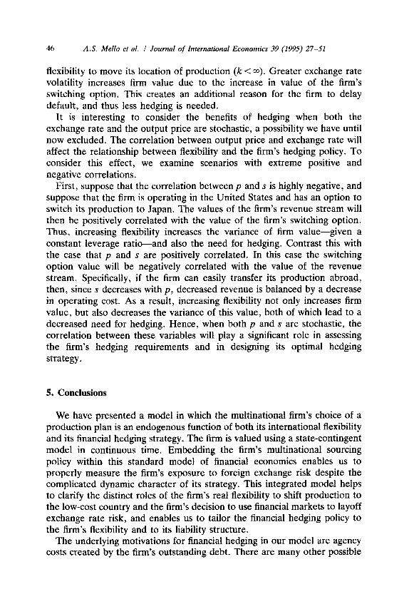
Fig. 4. Exchange rate volatility and efficient hedging. (a) Fixed nominal debt obligations, 6* = $1. (b) Fixed debt/value ratio = 29%. The efficient hedge for a firm is shown as a function of the firm’s flexibility/switching costs for different exchange rate volatilities. Constant exogenous parameters are p = $10.2, cuS = $10, cJ = Y 1000, ruS = 2%, r, = 2%, and a = 0. The current exchange rate is 0.01 $/U. Exchange rate volatility is constant as flexibility is varied. Results are shown for two different volatilities: W, = 10% and a, = 15%. In Fig. 4(a) the debt packages are constant in nominal terms as the flexibility changes: 6, = $1. In Fig. 4(b) the firm leverage ratios are held constant at 29% as flexibility changes.
upon the degree of flexibility, as the substitutes intuition and the results shown in panel A suggest, but also upon the relationship between the degree of flexibility and the structure of the firm’s liabilities-as the results shown in panel B underscore.
In Fig. 4 we illustrate the comparisons shown in Table 2, as well as the effect of changing the volatility of the exchange rate on the firm’s efficient hedge. It is interesting to note that increasing the volatility lowers the hedge required and decreases the value of efficient hedging. To understand this result, it is helpful to consider the special case of a firm operating in the United States and without any flexibility to shift production to Japan (k = w). Given a Iixed price greater than production costs, it is never optimal for an unlevered firm to exit the industry: SEE = ~0. Suppose, however, that the firm has some yen denominated debt outstanding, so that there is a finite exchange rate at which the equity owners would choose to default: s& < CQ. As v increases, the equity owners’ critical default rate rises: the value of the equity owners’ option on the firm is increasing in the volatility (T and they are more willing to continue servicing the debt in order to keep the option alive. So the equity owners’ optimal operating policy moves closer to the first best as exchange rate volatility increases, and less hedging is needed to induce the first-best operating policy. Suppose now that the firm has
46 A.S. Mella et al. i Journal of International Economics 39 (1995) 27-51
flexibility to move its location of production (k < m). Greater exchange rate volatility increases firm value due to the increase in value of the firm’s switching option. This creates an additional reason for the firm to delay default, and thus less hedging is needed.
It is interesting to consider the benefits of hedging when both the exchange rate and the output price are stochastic, a possibility we have until now excluded. The correlation between output price and exchange rate will affect the relationship between flexibility and the firm’s hedging policy. To consider this effect, we examine scenarios with extreme positive and negative correlations.
First, suppose that the correlation between p and s is highly negative, and suppose that the firm is operating in the United States and has an option to switch its production to Japan. The values of the firm’s revenue stream will then be positively correlated with the value of the firm’s switching option. Thus, increasing flexibility increases the variance of firm value-given a constant leverage ratio-and also the need for hedging. Contrast this with the case that p and s are positively correlated. In this case the switching option value will be negatively correlated with the value of the revenue stream. Specifically, if the firm can easily transfer its production abroad, then, since s decreases with pP decreased revenue is balanced by a decrease in operating cost. As a result, increasing flexibility not only increases firm value, but also decreases the variance of this value, both of which lead to a decreased need for hedging. Hence, when both p and s are stochastic, the correlation between these variables will play a significant role in assessing the firm’s hedging requirements and in designing its optimal hedging strategy.
5. Conclusions
We have presented a model in which the multination~ firm’s choice of a production plan is an endogenous function of both its international flexibility and its financial hedging strategy. The firm is valued using a state-contingent model in continuous time. Embedding the firm’s multinational sourcing policy within this standard model of financial economics enables us to properly measure the firm’s exposure to foreign exchange risk despite the complicated dynamic character of its strategy. This integrated model helps to clarify the distinct roles of the firm’s real flexibility to shift production to the low-cost country and the firm’s decision to use financial markets to layoff exchange rate risk, and enables us to tailor the financial hedging policy to the firm’s flexibility and to its liability structure.
The underlying motivations for financial hedging in our model are agency costs created by the firm’s outstanding debt. There are many other possible
A.S. Mello et al. I Journal of International Economics 39 (1995) 27-51 4-l
motivations for the firm to hedge foreign exchange risk. The technique developed here for incorporating agency costs within a dynamic model of firm valuation is very general, and other motivations for hedging could also be incorporated. This is one possible area for future research.
One important lesson from our analysis is that the correct hedge depends upon the nature of the firm’s flexibility, and so it is critical to have the right model of the firm’s competitive position and its relationship to exchange rate movements. We have modeled one specific form of multinational flexibility. It would be interesting to consider other market and industrial structures, for example the case in which the product market prices vary across countries and in which the firm is a monopolistic competitor.
Appendix
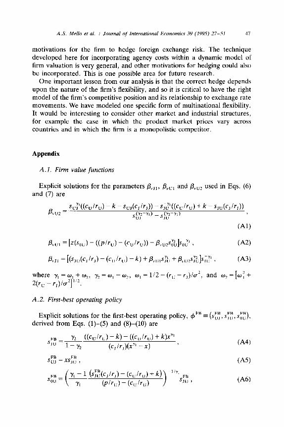
A.1. Firm value functions
Explicit solutions for the parameters pVJ1, pVul and pVUz used in Eqs. (6) and (7) are
P GNc”/r”> - k - s,,(c,/r,)) - Gx(c”~r”) + k - sJ”(cJ/rJ>) = vu2
where 0 G cx J 6 1. The value of the US subsidiary is the solution to the following two differential equations and associated three boundary con- ditions:
Three identities hold at the key switching points. The identity for the default switch point was given in the text, Eq. (11). The remaining two identities are
eJ(sUJ; 4) = e”(s,,; +I+ k , (~23)
e"(s,,; 4) = e'(s,,; 4) + k . (~24)
The following three additional boundary conditions are defined by first- order conditions at the equity owners’ optimal switching points:
ej*G,; +*I = e,U*(s:,; +*I, (A251
eJ*(&; 4*) = eY*(s,*,; 4*> , (A261
e,U*(s&; c$*) = 0. (~27)
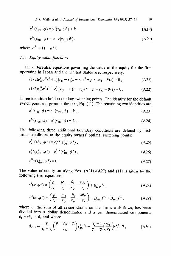
The value of equity satisfying Eqs. (A21)-(A27) and (11) is given by the following two equations:
WW
where 8, the sum of all senior claims on the firm’s cash flows, has been divided into a dollar denominated and a yen denominated component, f3, + 80, = 8, and where
P eU1 =~(p-~-e~)sf;y~-~(~)s~~-y~, (A30)
50 A.S. Mello et al. I Journal of International Economics 39 (1995) 27-51
(A31)
(~32)
The explicit solutions for the equity owners’ optimal operating policy also derived from Eqs. (Al@-(A24) and (11) are
Y2 ST” = 1 - y2
((cu /‘“I - k) - ((cu l’u) + QY1
(c, Ir,)(xY’ - x) ’ (A33)
‘UJ * =xs,*,, (A34)
s&J = 9s;” 7 (A35)
where ‘q solves the non-linear equation
P-G-% -- TU
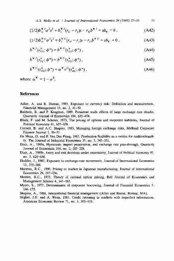
A 5 Bond values
All non-equity securities are valued taking the equity owners’ optimal operating policy, c#J*, as given. Suppose, for example, that the firm has a set of bonds (perpetuities) outstanding, with annual obligations in dollars and yen of 6, and 6,, respectively, and that these are the only outstanding obligations. The dollar denominated bonds satisfy the following set of equations:
Adler, A. and B. Dumas, 1983, Exposure to currency risk: Definition and measurement, Financial Management 13, no. 2, 41-50.
Baldwin, R. and P. Krugman, 1989, Persistent trade effects of large exchange rate shocks, Quarterly Journal of Economics 104, 635-654.
Black, F. and M. Scholes, 1973, The pricing of options and corporate liabilities, Journal of Political Economy 81, 637-659.
Cornell, B. and A.C. Shapiro, 1983, Managing foreign exchange risks, Midland Corporate Finance Journal 1, 16-31.
De Meza, D. and F. Van Der Ploeg, 1987, Production flexibility as a motive for multinationali- ty, The Journal of Industrial Economics 35, no. 3, 343-351.
Dixit, A., 1989a, Hysteresis, import penetration, and exchange rate pass-through, Quarterly Journal of Economics 104, no. 2, 205-228.
Dixit, A., 1989b, Entry and exit decisions under uncertainty, Journal of Political Economy 97, no. 3, 620-638.
Hodder, J., 1982, Exposure to exchange-rate movements, Journal of International Economics 13, 375-386.
Marston, R.C., 1990, Pricing to market in Japanese manufacturing, Journal of International Economics 29, 217-236.
Merton, R.C., 1973, Theory of rational option pricing, Bell Journal of Economics and Management Science 4, 141-183.
Myers, S., 1977, Determinants of corporate borrowing, Journal of Financial Economics 5, 146-175.
Shapiro, A., 1988, International financial management (Allyn and Bacon, Boston, MA). Stiglitz, J.E. and A. Weiss, 1981, Credit rationing in markets with imperfect information,